una presentacion de los minimos cuadrados generalizados, y

REVISTA INVESTIGACIÓN OPERACIONAL VOL., 32 , NO. 1, 67-89, 2011
Novedades de software/New softwares
UNA PRESENTACION DE LOS MINIMOS
CUADRADOS GENERALIZADOS, Y EN
PARTICULAR, PARA FUNCIONES VECTORIALES
Jorge Lemagne Pérez 1
Departamento de Matemática Aplicada Facultad de Matemática y Computación, Universidad de La Habana
ABSTRACT
In this communication, a critical bibliographical survey on discrete least squares (LS) presentation is firstly made, and
especially of data fitting (DF).
Afterwards, to help to overcome part of the limitations and deficiencies that were shown in the bibliography, a formal
presentation of generalized least squares (GLS, in general non linear by default) is made, and very especially of DF for vector
valued functions (VVF); the corresponding non linear system of equations, extension of the well known normal equations, is
derived. From there, some particular cases are obtained, for example, when the function is real valued, and when the
approximation is linear. This second example is just linear generalized least squares (LGLS).
KEY WORDS: Data fitting, least squares, multivariate methods, normal equations, Generalized least squares
MSC: 65F30
RESUMEN
En esta comunicación se hace, primeramente, una revisión crítica de cómo se presenta el tema de mínimos cuadrados (MC, se
sobrentiende discretos) en la bibliografía existente, y en particular, del ajuste de datos (AD).
Posteriormente, para contribuir a superar parte de las limitaciones y deficiencias señaladas en la revisión bibliográfica, se hace
una exposición formal del problema de mínimos cuadrados generalizados (MCG, se sobrentiende no lineales en general), y muy
en especial del AD para funciones vectoriales (FV); se deduce el sistema no lineal de ecuaciones correspondiente, extensión del
conocido sistema de ecuaciones normales. A partir de ahí se deducen algunos casos particulares, entre ellos, cuando la función
toma valores reales, y cuando la función de aproximación es lineal, o sea mínimos cuadrados generalizados lineales (MCGL).
1. INTRODUCCION. UNA REVISIÓN BIBLIOGRÁFICA CRÍTICA SOBRE MÍNIMOS
CUADRADOS
Por su importancia, los MC son tratados con gran frecuencia en numerosas publicaciones científicas y técnicas.
Es necesario señalar que el problema de MC es conocido bajo diferentes nombres en varias ramas; por
ejemplo, en Estadística se le llama análisis de regresión, y en Ingeniería, estimación de parámetros, filtraje o
identificación de procesos.
De acuerdo con los objetivos de la presente investigación, resulta conveniente hacer – en primer lugar – una
revisión crítica de diferentes presentaciones de este tema, y específicamente sobre AD. Dentro de la
bibliografía existente, se consultaron no menos de 140 publicaciones (vea 9).
Primeramente nos referiremos al problema de AD mediante MCP, después se aborda MCG para funciones que
toman valores escalares, y posteriormente MCG para FV, culminando de esta manera con el caso general en
que se quieran aproximar funciones
p q
f : ℜ → ℜ , p ≥1
, q ≥ 1.
(1.1)
A partir de toda esta panorámica se destacan las limitaciones de los enfoques en las publicaciones, incluyendo
un breve ejemplo práctico para resaltar dichas insuficiencias.
1 lemagne@matcom.uh.cu
67

El software existente sobre MCG será analizado en una publicación posterior.
1.1.Ajuste de datos mediante mínimos cuadrados ponderados
Aquí podemos suponer, sin pérdida de generalidad, que q = 1 .
En particular, el caso lineal es clásico dentro del Análisis Numérico, no presenta dificultades (desde el punto
de vista teórico), y existen programas para computadoras que lo resuelven. Es abundante la bibliografía donde
el problema de MC se trata a lo sumo con ese enfoque, pero tomando p = 1;
véase por ejemplo las obras de
Berezin [1971], Gautschi [1997], Gill et al [1990], González [1983], Guerra et al [1987], Isaacson y Keller
[1971], Kincaid et al [1995], Ralston [1965], Sastre [1988] y Volkov [1990]; en la inmensa mayoría de los
casos se considera la función de peso como la constante 1, lo que lo convierte en un problema de mínimos
cuadrados ordinarios (MCO).
Específicamente González y Guerra sólo consideran ajustes mediante rectas, e Isaacson y Keller mediante
polinomios y polinomios trigonométricos.
Otros casos más generales son menos estudiados:
1. El caso no lineal no aparece tratado con tanta frecuencia en la bibliografía:
Aquí incluiremos las publicaciones de Tellinghuisen [2005] y Rufino et al [2005].
Un clásico como Forsythe et al [1972] hace una breve incursión cuando p = 1 y señala que se limitará a la
aproximación de funciones de una variable real, ya que la teoría de la aproximación de funciones de varias
variables no está bien desarrollada. Carleton parte de que p = 1.
Se considera fundamentalmente el caso
lineal, pues el no lineal apenas se estudia. Koroliuk [1981] se limita a formular el problema. Es interesante
señalar que Bolshakov [1989] en caso necesario linealiza el problema mediante serie de Taylor. Raíces [1986]
considera de manera restringida el orden de la aproximación, aunque posteriormente sí hace el desarrollo
general para deducir el sistema no lineal de ecuaciones que hay que resolver. El libro de Motulski y
Christopoulos [2003] está orientado a los investigadores y es muy práctico; la regresión múltiple sólo la trata
ligeramente. En Mahata [2003] se exploran propiedades estadísticas asintóticas de los estimados obtenidos
mediante mínimos cuadrados no lineales separables.
2. El caso lineal p ≥1
, naturalmente aparece más tratado, pero sin la suficiente generalidad y sistematización:
Forsythe et al casi sólo menciona la regresión múltiple y no profundiza en ella. En Linares [1986] y Suárez
[1988] aparecen algunos casos de aproximación lineal multivariada, pero esto no se enfoca deductivamente a
partir de una aproximación lineal general (con p variables independientes). Cué, Castell, [1987], Cué et al
[1985] aunque consideran funciones de regresión más generales que los dos autores anteriores, tampoco las
enfocan como casos particulares de aproximación lineal general.
En Tamayo [1984] sí aparece un análisis bastante general de este caso, pero no se dice explícitamente que se
p
trabaja con funciones deℜ
en ℜ , ni se expresa la matriz del sistema de ecuaciones normales en términos de
los productos escalares generalizados a este tipo de funciones. Tampoco se estudian las propiedades de dicho
sistema de ecuaciones lineales. Keller [2002] y Stanford [2000] tratan el caso particular de MCO, a partir
directamente de los elementos de la matriz del sistema sobredeterminado, y por tanto no necesitan tomar en
cuenta a p . Hager [1988], Koroliuk [1981], Lawson [1995] y Wilkinson [1971] también consideran MCO,
pero sin hacer referencia explícita alguna a función empírica. Entonces, como primera conclusión, podemos
afirmar que la mayor parte de la bibliografía sobre el tema aborda MCO o MCP, pero inclusive dentro de cada
variante, no se hace un análisis lo suficientemente general. La abundancia de información sobre esos tópicos
específicamente, se justifica en parte por el hecho que son los más sencillos y donde los métodos
computacionales son más eficientes.
1.2. Ajuste de datos mediante mínimos cuadrados generalizados
68

Según Schwetlick [1991], “la estimación no lineal de parámetros es tanto interesante matemáticamente como
útil en la práctica, y muchos resultados nuevos pueden esperarse en el futuro.”
En CAC-2002 se dice que “Aunque la incertidumbre en las mediciones es parte esencial de las mediciones
químicas, la mayoría de los métodos multivariados de calibración ignoran este factor importante, al suponer
implícitamente error uniforme no correlacionado o intentar acomodar el comportamiento del error durante el
pre-procesamiento rutinario.”
Smith [1993] afirma:
“…, existen formulaciones de este método (mínimos cuadrados) más avanzadas y menos frecuentemente
consideradas que merecen tomarse en cuenta. Estas ofrecen posibilidades para la manipulación y utilización de
datos, que en general no son apreciadas adecuadamente por la comunidad científica. En particular, es posible
considerar problemas no lineales, incluir datos ponderados y correlacionados, permitir la existencia de
información previa acerca de los parámetros buscados,…”
A partir de la lectura de los párrafos anteriores, resulta comprensible que haya relativamente muchas menos
publicaciones sobre MCG (como dijimos, se sobrentiende no lineales en general).
Según Reilly [1998] hasta el momento no existe una definición universal de MCG. En su opinión, podría
interpretarse como una extensión de la aplicación de los MC a un problema más general que el caso más
sencillo en que los errores tienen media constante, varianza constante y no están correlacionados, en otras
palabras, una extensión hacia lo que ocurre en la realidad.
Esa falta de definición universal de MCG constituye una de las dificultades para la realización de esta
investigación.
No obstante, posteriormente daremos una definición rigurosa de MCG.
En Arras [2003] se hace una aplicación de los MC. Con respecto a los MCG, sólo se menciona su utilización,
sin incursionar en los detalles matemáticos. Dicha aplicación está orientada al campo de la Robótica y en la
misma se utilizan coordenadas polares para obtener finalmente fórmulas cerradas de los valores de los
parámetros óptimos. Por tanto, su enfoque difiere del de esta comunicación. No se menciona explícitamente
ningún software específico para resolver los problemas numéricos.
En general, las publicaciones incluidas en este grupo consideran MCG, pero no trabajan con FV, pues
consideran q = 1.
Además, la mayoría considera aproximaciones lineales (MCGL), y en algunos casos se
incluye una breve nota para no lineales.
1.3. Caso de MCG
Aquí podemos incluir a Marsily et al [2000], y Davidson y MacKinnon [1999]. IAEA [2003] hace sólo una
referencia a los MCG.Milton et al [2006] constituye una aplicación de los MCG a un problema de calibración.
Bultheel et al [2001] construyen una matriz de pesos que es diagonal por bloques. Madsen y Nielsen [2005]
hacen sólo una breve incursión a los MCG a partir de propiedades de la matriz de varianza y covarianza;
posteriormente incluyen la restricción que la misma tiene que ser definida positiva. La función de
aproximación puede ser no lineal, y en este caso se utilizan algoritmos del tipo Gauss-Newton, basados en
linealizaciones sucesivas. No se mencionan funciones vectoriales empíricas. En Eisenberg y McLaughlin
[2001] el procedimiento para la estimación está basado en un enfoque bayesiano de los MCG. Los parámetros
y estados estimados son considerados funciones aleatorias del espacio y/o del tiempo con distribuciones
previas o esperadas.
Similarmente, tanto en IAEA [2007] como en Smith [1993] se explican los fundamentos del método de MC
desde ese mismo punto de vista; en ambas se utiliza un modelo que ha sido linealizado. En Smith aparece un
programa para MCG 2 .
2 En una futura publicación, se comentará más al respecto.
69

1.4. Caso de MCGL
La tesis de Van Donkelaar [2000] (un enfoque flexible de la parametrización lineal) utiliza un procedimiento
similar al de los MCG. IAEA [2004] y Thisted [1988] estudian los MCGL para q = 1 . Safi y White [2006]
hacen una comparación entre MCO y MCG, ambos lineales; no consideran funciones vectoriales empíricas.
García [1995] los trata muy brevemente utilizando función experimental; similarmente Nathan [2002], pero
con mayor amplitud. Chatterjee y Hadi [2006] en un capítulo especial tratan el caso en que los errores están
correlacionados, pero los datos que se ajustan son escalares y esto se hace mediante modelos lineales. En
Hengl [2007] sólo se hace referencia a los MCG lineales, y aún así se plantea que “…Ningún sistema GIS
(Geographical Information System) incluye todo acerca de modelos generalizados lineales,...” Hart y Matt
[1996] tiene una breve nota al respecto. El software al cual hace referencia es para MCO lineales, por lo que
habría que reformular el problema previamente. En Ngo [2006], la estimación de los parámetros desconocidos
se realiza utilizando el método estándar de máxima verosimilitud. Se consideran funciones vectoriales, pero
mediante un modelo lineal, siendo independientes las mediciones de diferentes individuos. Además, se exige
que la matriz de covarianza de cada individuo (correspondiente a mediciones repetidas) sea definida positiva.
Desde el punto de vista conceptual, Lindegren [2006] considera que en los MC no lineales la matriz de
covarianza es diagonal y que los MCG son lineales. Robison-Cox [1998] y Ripley [1998] no toman en cuenta
que la matriz V de varianza y covarianza pudiera ser singular. Tanto Hengl et al [2004] como Qin [2006] se
refieren a los MCG lineales considerando la expresión matricial del vector óptimo de parámetros, donde se
exige que la matriz de covarianza sea no singular; no se utilizan funciones vectoriales. A manera de resumen,
en general las publicaciones incluidas en este subepígrafe consideran MCG, pero no trabajan con FV. Además,
la mayoría se refiere a aproximaciones lineales, y en algunos casos se incluye una breve nota para no lineales.
1.5. Ajuste de datos mediante mínimos cuadrados generalizados para funciones vectoriales
Continuando con este orden descendente en abundancia bibliográfica, llegamos al extremo cuando queremos
incursionar en AD mediante MCG para FV (abreviadamente AD_MCG_FV, principal objetivo nuestro), sobre
todo cuando buscamos una formulación de este problema.
Existen aplicaciones donde es necesario trabajar con funciones f del tipo (1.1). Podría pensarse en la
p
descomposición de f en funciones fL
: ℜ → ℜ , L = 1,
K,
q (cada L denota una característica distinta)
para analizar cada f L independientemente (de manera univariada con respecto a las variables dependientes).
Sin embargo, este principio no es directamente aplicable a los MCG, por las correlaciones existentes entre las
distintas características.
Nota: De ahora en adelante, cuando hablemos de característica, se sobreentiende que es con respecto a las
variables dependientes.
Hagamos también aquí una incursión a las publicaciones relacionadas con este tópico:
En Carpenter y Kenward [2007] se hace brevemente una aplicación de los MCG al análisis multivariado.
Sobre series de tiempo: En su caso más complejo, las series de tiempo permiten la modelación simultánea de
múltiples series dependientes. Este problema es al mismo tiempo poco frecuente y costoso, por lo que resulta
natural desarrollar métodos para contribuir a automatizar el proceso (Forecasting [1997, (2)]). (La citada
publicación no añade nada más sobre este caso múltiple). Pourahmadi [2002] trata algo sobre series de tiempo,
pero con modelos lineales. Gallant [2000] supuestamente formula el problema de MCG a partir de una suma
de formas cuadráticas, y no de una forma cuadrática, como haremos nosotros. En realidad, la formulación
corresponde al AD_MCG_FV y no al problema general de MCG. Después brevemente sólo da una idea
introductoria de cómo se podrían deducir las propiedades principales. Debemos señalar que, en la
transformación al caso univariado, la vectorización se hace de manera informal; además la matriz de varianza y
covarianza se toma de manera bastante restringida (sobre este último aspecto volveremos después). Además
de Gallant, Cué et al [1985], Marangoni [1999], Multiresponse [2003] y Saha [2003] también abordan la
aproximación con multirespuestas. Cué et al tratan sólo el caso lineal, y consideran un vector de parámetros
para cada característica, lo que no corresponde con el enfoque de esta investigación. Marangoni sólo se refiere
70

a la formación de la matriz de varianza y covarianza. Multiresponse minimiza E E
T
, donde E es la matriz
error en la aproximación. Saha hace una breve explicación del modelo multirespuestas no lineal, sin introducir
MC. A continuación pasa al modelo multirespuestas lineal, y da el estimador que coincide con la solución de
MCGL.
2. LIMITACIONES QUE PUEDEN EXISTIR EN LA MATRIZ DE VARIANZA Y COVARIANZA
En Gallant, Cué et al, Marangoni, Multiresponse y Saha, (publicaciones todas referenciadas en el epígrafe
anterior), la matriz de varianza y covarianza V tiene la forma:
V = Σ ⊗ I
(2.1)
Esto trae como consecuencia 2 restricciones:
1. Se consideran correlaciones sólo entre características de una misma observación o “individuo”.
(R1)
2. Dadas 2 características determinadas, las covarianzas correspondientes a cada uno de los individuos
son todas iguales.
En algunos problemas las restricciones anteriores, (R1) y (R2) podrían constituir una seria limitación.
Consideremos el siguiente ejemplo de Meteorología:
En (1.1) hagamos p = 3 , q = 4 , y f ( x,
y,
z)
= ( P,
vx
, vy
, vz
) , donde x , y , z , son las
coordenadas de un punto de la atmósfera; P , v x , y v , v z , denotan respectivamente la presión y las
componentes de la velocidad del viento en cada uno de los ejes cartesianos, todos correspondientes al punto de
la atmósfera en cuestión.
Se sabe ─ por ejemplo ─ que la velocidad del viento apunta hacia el lugar de menor presión; por tanto entre
puntos distintos de la atmósfera existen correlaciones entre P y las componentes del viento.
Las consideraciones anteriores nos hacen buscar un modelo más general que el multivariado correspondiente a
(2.1).
3. LIMITACIONES GENERALES
Al tomar en consideración los aspectos expuestos en los epígrafes anteriores con respecto a la bibliografía
sobre MC, y más específicamente AD, podemos señalar como conclusión las siguientes limitaciones:
1. En las publicaciones donde se presenta el modelo multirespuestas con algún grado de formalidad,
generalmente existen las restricciones (R1) y (R2), y se supone que V es definida positiva (sin admitir
singularidad).
2. Existe una tendencia a considerar AD sólo para funciones que toman valores escalares, o sea q = 1.
Si bien es cierto que cuando q > 1 puede hacerse una conversión del problema a MCO, el caso general q ≥ 1
necesita una formulación propia como problema de origen, e inclusive hay algunas aplicaciones que lo
requieren.
3. No existe una formalización del AD con el suficiente grado de generalidad, es decir del
AD_MCG_FV. Es más, con frecuencia (véase Gallant, Thisted, Davidson y MacKinnon poner el año o el
número de orden) el problema más general de MCG se reduce ─ lamentablemente ─ al de AD.
4. No existe tampoco un enfoque deductivo y orgánico del problema, es decir desde lo más general
hasta casos particulares más conocidos. En este sentido la información se encuentra bastante dispersa.
5. No es costumbre considerar que este problema general es además parte del Análisis Numérico y que
es posible darle un enfoque natural dentro de esta disciplina también.
71

4. ¿POR QUE UNA PRESENTACION?
La presentación que haremos aquí tiene pues como objetivo contribuir a superar las limitaciones y deficiencias
señaladas en el epígrafe anterior. 3
Para comprender mejor los pasos que se han seguido en la misma, véase el diagrama que aparece más abajo; la
enumeración de los bloques corresponde con el orden de los pasos, el final de cada flecha es un caso particular
deducido en el trabajo a partir del comienzo de la flecha.
Para cada bloque se ha hecho la formulación del problema correspondiente y la deducción del sistema de
ecuaciones que resulta de plantear la condición necesaria de mínimo local.
Los casos más elementales, correspondientes a MCO y MCP fueron tratados en las publicaciones de Lemagne
[2000] y [2001] respectivamente, y por lo tanto no serán abordados aquí. Ambas comunicaciones sirvieron de
base para el desarrollo de esta investigación.
De acuerdo con el § 3, a través de la presentación llegaremos a nuevos resultados utilizando algunos ya
conocidos pero que aparecen en la bibliografía de manera dispersa e informal.
5. MINIMOS CUADRADOS GENERALIZADOS
5.1 Caso no lineal en general
n+
1
Sea r : ℜ → ℜ , función no lineal (se sobreentiende en general), k = 0, K,
N ,
k
MCG
MCG
AD, q ≥1
MCG
AD, q = 1
(1)
(3)
(4)
+ 1
∈ℜ n
c , y denotaremos este vector como c ( c j ) j = 0, K,
n
72
MCGL
MCGL
AD, q ≥1
MCGL
AD, q = 1
= (5.1)
3 Recordemos también que el software existente sobre MCG será analizado en una publicación posterior.
(2)
(5)
(6)

Consideremos ahora la función vectorial
( k ) k N c r c r ( ) = ( ) , (5.2)
= 0,
K,
y la matriz W = ( wi
k ) , que supondremos que es simétrica y definida no negativa.
i,
k = 0,
K,
N
Se quiere entonces:
minimizar (c)
Los parámetros c j deben ser determinados para alcanzar dicho objetivo.
El problema anteriormente formulado es el de MCG.
T
E : E(
c)
= r ( c)
W r(
c)
(5.3)
+ 1
Nota: En general, basta que todas las r k estén definidas en un cierto conjunto S , acorde con la
definición más general de función parcial, aunque en la práctica matemática común es costumbre trabajar con
funciones totales o aplicaciones.
73
⊆ ℜ
n
Debido a la descomposición de Cholesky de W (Hart y Matt [1996]), en (5.3) efectivamente se minimiza una
suma de cuadrados.
En algunas ocasiones – para abreviar – suprimiremos la c .
En la bibliografía consultada no aparece ninguna demostración de la condición necesaria de mínimo local. Sin
embargo, apliquemos el siguiente resultado brindado por Scales [1985] para derivar funciones cuadráticas de
varias variables; estas son de la forma:
1 T T
F(
x)
= 2 x Ax + b x + c
De acuerdo con la obra citada, el gradiente de la función anterior es
g ( x)
= A x + b
En primer lugar, hagamos b = 0 , c = 0 . Entonces
∂F
= a j • ⋅ x
∂ x j
Hagamos además x = r , A = W , E = 2F
, y apliquemos regla de la cadena:
Como j varía entre 0 y n , resulta que:
∂E
∂ c
j
=
= 2
∂E
∂ r
N
k
∑ ⋅
k = 0 ∂ rk
∂ c j
∂ r
N
k
∑ wk
• ⋅ r ⋅
k = 0 ∂ c j
⎡ N ∂ r ⎤
k
= 2 ⎢∑
wk
• ⎥ r
⎢⎣
k = 0 ∂ c j ⎥⎦
⎡ ∂ r ⎤
= 2 ⎢ ⋅W
⎥ r = 0
⎢⎣
∂ c ⎥⎦
T
j

es la matriz jacobiana de (c)
J T
J (c)
es una matriz de N + 1 filas y + 1
( c)
Wr(
c)
= 0
74
:
⎛ ⎞
J ( c)
⎜
∂
= rk
( c)
⎟
(5.4)
⎜ c ⎟
⎝ ∂ j ⎠
k = 0,
K,
N
j = 0,
K,
n
r . ■
n columnas. Observe además que r es ortogonal a cada columna
de WJ , por lo que llamaremos al sistema anterior sistema de ecuaciones normales (SEN). El mismo se ha
definido aquí de una manera más general que la usual, pues es costumbre restringir la definición a r(c) lineal
y W = I .
5.2 Mínimos cuadrados generalizados lineales
En (5.1) supongamos que las rk (c)
son funciones lineales, o sea:
donde los a k m y los b k son números conocidos.
Sea
Entonces
Sustituyendo en (5.2)
r(
c)
=
Haciendo b = ( bk
) , tenemos que
k = 0, K,
N
Luego, nuestro problema consiste en
n
∑
m=
0
r ( c)
= b − a c , (5.5)
k
A =
k
( a )
k m k = 0,
K,
N
m = 0,
K,
n
rk ( c)
bk
− ak
= •
⋅ c
k m
( b ) − ( a ) ⋅ c
k k = 0,
K , N k • k = 0,
K,
N
T
minimizar ( b − Ac)
W ( b − Ac)
El SEN correspondiente se obtiene a partir de (5.4) y (5.5):
J ( c)
=
m
r = b − Ac
(5.6)
( − a ) = − A
k j
k = 0,
K , N
j = 0,
K,
n
Aplicando (5.6), el SEN es:
A W[
b − Ac]
= 0
T
,
o equivalentemente
T
T
A WAc
= A W b
(5.7)
Como puede verse, la matriz de este sistema es simétrica y definida no negativa. ■
Es significativo señalar que en este epígrafe sobre MCG y su caso particular MCGL, no hay que hacer (de
manera contraria a lo que suele encontrarse en la bibliografía) referencia alguna a función experimental. Esta
referencia comienza a partir del próximo epígrafe:

6. AJUSTE DE DATOS MEDIANTE MINIMOS CUADRADOS GENERALIZADOS PARA
FUNCIONES VECTORIALES
6.1 Formulación del problema
p q
p
q
Sea f : ℜ → ℜ , una función desconocida en la práctica ( p ≥1, q ≥1)
; xk ∈ ℜ ; f k ∈ ℜ y se
conoce empíricamente, siendo f k una aproximación al vector desconocido f ( xk
) , ( k = 0,
K,
N)
.
p q
F : ℜ → ℜ es una función de aproximación a f , F ( x)
= F(
x;
c)
donde c fue definido en (5.1).
De acuerdo con el párrafo anterior, sea fkL la componente L -ésima del vector f k . Además, por ser F una
p q
función de ℜ en ℜ , esta puede descomponerse en las funciones ℜ → ℜ
p
F L : , L = 1, K,
q .
Adoptemos las notaciones:
rkL ( c)
= f kL − FL
( xk
; c)
(6.1)
R L ( c)
= ( rkL
( c)
) (6.2)
k = 0,
K,
N
Ahora hagamos
⎛ R1(
c)
⎞
⎜ ⎟
⎜ R2
( c)
⎟
r = ⎜ M ⎟
⎜ ⎟
⎜ ⎟
⎝ Rq
( c)
⎠
y sea W una matriz cuadrada de orden ( N + 1)
q , simétrica y definida no negativa.
Entonces, el problema de AD mediante MCG para FV (abreviadamente AD_MCG_FV) consiste en, con las
suposiciones anteriores, realizar (5.3).
Observe que rkL (c)
representa la desviación de la aproximación ( x ; c)
, y además que cada RL (c)
es un vector columna de N + 1 elementos.
75
FL k con respecto al dato empírico f kL
De manera similar a lo señalado en la nota del § 5.1, f y F pueden ser funciones parciales definidas
totalmente sobre el mismo conjunto.
6.2 Sistema de ecuaciones normales
Para la formulación anterior vimos que se realizó una partición del vector columna r . Con el fin de obtener la
forma particular de (5.4), y posteriormente profundizar en cómo definir la matriz W , realizaremos también
particiones de J y de W :
⎛ J1
⎞
⎜ ⎟
⎜ J 2 ⎟
J = ⎜ = ( J L ) L = 1,
K,
q
M ⎟
⎜ ⎟
⎜ J ⎟
⎝ q ⎠
Cada J L es la matriz jacobiana de R L , y tiene N + 1 filas y n + 1 columnas. Por (6.2):
⎛ ⎞
J L ( c)
⎜
∂
= rk
L ( c)
⎟
(6.3)
⎜ c ⎟
⎝ ∂ j ⎠k
= 0,
K,
N
j = 0,
K,
n

⎛W11
⎜
⎜W21
W = ⎜ M
⎜
⎝Wq1
W12
W22
M
Wq2
L
L
O
L
W1q
⎞
⎟
W2q
⎟ ( WL
H )
M ⎟ =
(6.4)
L = 1,
K,
q
⎟
H = 1,
K,
q
W ⎟
qq ⎠
W es un bloque cuadrado de orden N + 1,
y por ser W simétrica se cumple que
Cada L H
HL W W = (6.5)
Sustituyendo en (5.4), tenemos que:
T [ ( J L ) ] ( W ) ( ) = 1 , , LH R
L K q
L = 1,
K,
q H H = 1,
K,
q = 0
H = 1,
K,
q
76
T
LH
q
T
T ⎛ ⎞
[ ( J ) ] ⎜ W R ⎟ = 0
L
L = 1 , K , q
⎜
⎝
q
∑
H = 1
L H
H
⎟
⎠
L = 1,
K,
q
q ⎡ T ⎤
⎢J
L WL
H RH
⎥ = 0
(6.6)
⎣ H ⎦
∑ ∑
L = 1 = 1
q
q
∑∑
L = 1 H = 1
T
L
J W R = 0 , (6.7)
L H
que puede interpretarse como una versión por bloques del SEN (5.4).
Este sistema también puede escribirse así:
Al aplicar (6.5):
q
∑
L = 1
q
∑
L = 1
J
J
T
L
T
L
W
W
q
∑
1 = L
L L
L L
R
R
L
L
q
T
∑ J L
L,
H = 1
H < L
H
q
T
J L
L,
H = 1
H > L
+ WL
H RH
+ ∑
q
L,
H = 1
H < L
q
T
J H
H , L = 1
L > H
T
+ ∑ J L WL
H RH
+ ∑
q
, 1
< =
H L
H L
W
W
LH
T
L H
R
H
R
L
= 0
= 0
T
T T
[ J W R + J W R ] = 0
T
J L WL
L RL
+ ∑ L L H H H L H L
(6.8)
En esta última versión del SEN, con respecto a la estructura por bloques (6.4) de W , sólo intervienen los
bloques de la diagonal y los que están por debajo de ella.
Si W es diagonal por bloques, desaparece la segunda sumatoria.
En la bibliografía consultada no aparece reflejado ningún planteamiento del SEN cuando se realiza
AD_MCG_FV.
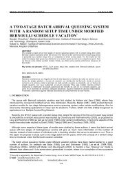
6.3 EJEMPLO 4
Sea
2 2
u − v
f : ℜ → ℜ ; f ( u,
v)
= ( sen(
u + v),
e )
4
Este sencillo ejemplo es un tanto idealizado, pero ilustra convenientemente los anteriores desarrollos
matemáticos.

De esta función se han extraído los valores siguientes:
Considere ahora
con
3
2.5
2
1.5
1
0.5
0
( u, v)
f ( u,
v)
0 0 0 1
0 1 ( 1)
1 0 ( 1)
F(
u,
v;
c , c ) =
0
1
⎛4
⎜
⎜0
⎜1
W = ⎜
⎜1
⎜
⎜
0
⎜
⎝1
sen −1
sen e
c 1 ( u−v
)
( c sen(
u + v),
e )
0
1
0
0
1
0
0
de tal manera que realice AD_MCG_FV (en este ejemplo W es definida no negativa, pero singular). Por
c ; c 1.
Veremos lo que sucede.
1
0
2
0
0
1
77
1
0
0
2
0
1
0
1
0
0
1
0
1⎞
⎟
0⎟
1⎟
⎟
1⎟
0
⎟
⎟
4⎟
⎠
supuesto, al resolver este problema debe obtenerse aproximadamente 0 = 1
En este caso
1
0.8
f1(u,v)=sen(u+v)
f2(u,v)=exp(u-v)
0.6
0.4
V
0.2
0
-0.2
p = 2 ; q = 2 ; N = 2 ; = 1
e
n .
Denotemos s = sen(1) . De acuerdo con (6.8), el SEN correspondiente es:
⎛
2 −1
2 −c
1 c 1
⎜
− 3s
− se − se + 3s
c0
+ se + se
⎜ −c
1 −c
1 −c
1−1
− 2c
1 c 1 c 1 c 1
⎝ se − sc0e
+ e − e − se + sc0e
− 4e
-0.2
0
0.2
U
0.4
0.6
0.8
1
f2
f1
1.2
+ 1
1=
+ 4e
2 c 1
⎞ ⎛0⎞
⎟ = ⎜ ⎟
⎟
⎠ ⎝0⎠

Con el cambio de variable
c 1
y = e , el sistema anterior es equivalente a:
1 ⎡ −1
1 ⎤
c 0 = ⎢3s
+ e + e − − y
3s
⎥
⎣
y ⎦
− 2 e +
2
2 − e y +
2
1−
11e
3
y + 11e
y
4
( ) ( ) = 0
Obviamente y = e es raíz de la segunda ecuación; pero por la regla de los signos de Descartes, esta no tiene
más
■
raíces positivas. Por lo tanto, el sistema sólo se satisface para c 0 = 1;
c 1= 1.
6.4 CALCULO DE LA MATRIZ W
Aunque en la definición de AD_MCG_FV puede tomarse libremente cualquier W que cumpla las condiciones
+
generales especificadas, en la práctica es usual hacer W =V , o sea la pseudoinversa de V (Gill et al
[1990]), donde V es la matriz de varianza y covarianza de las observaciones.
Para formar la matriz V , consideramos una partición similar a la que hicimos con W , es decir:
V = V
donde V LH es un bloque cuadrado de orden N + 1 .
( )
L H L = 1, K,
q
H = 1,
K, q
Dentro de V LH , el elemento de posición ( k, j)
es la covarianza entre el valor de la característica L en la
, = 0,
K .
observación o “individuo” k , y el valor de la característica H del individuo j ; k j , N
7. ALGUNOS CASOS PARTICULARES
7.1 AJUSTE DE DATOS MEDIANTE MINIMOS CUADRADOS GENERALIZADOS PARA
FUNCIONES QUE TOMAN VALORES ESCALARES
En este caso, q = 1 , f k es un escalar, y para cada x k y cada c , F( xk
; c)
también lo es.
R 1 es sencillamente r (o sea, el residual tal como se conoce comúnmente).
W es una matriz simétrica y definida no negativa de orden N + 1 .
Nuestro problema particular consiste entonces, con estas especificaciones, en (5.3). Para hallar el SEN,
notemos que en cada una de las sumatorias de (6.6) queda un solo sumando, y los índices L y H pueden
eliminarse:
J W R = 0
T
1
J T
11
78
1
W r = 0
lo que naturalmente concuerda con la ecuación general (5.4).
Podría parecer que a partir de este último caso, más frecuentemente utilizado, puede llegarse mediante alguna
reformulación al AD_MCG_FV, del § 6.1 (para q > 1 ). En general no es así, pues habría que tener más de
una F L , y cada una de ellas debe ser evaluada en todos los x k , mientras que aquí disponemos a tal efecto de
una sola F L .
,

Conclusión: En general, desde el punto de vista de formulación del problema, no basta trabajar con
funciones que tomen valores escalares. El AD_MCG_FV no es – por tanto – un problema trivial, y requiere
formalización propia.
7.2 AJUSTE DE DATOS MEDIANTE MINIMOS CUADRADOS GENERALIZADOS LINEALES
PARA FUNCIONES VECTORIALES
Supongamos ahora que en la formulación de AD_MCG_FV, hacemos q ≥1
y además supongamos que F
depende linealmente de los parámetros c m , o sea que
n
∑ m
m = 0
F(
x;
c)
= c φ ( x)
,
( ) =
79
m
p
x∈ ℜ
(7.1)
para una familia de funciones { φ m x } m
p
prefijada, φ 0,...
n
m : ℜ
q
→ ℜ . Note que esta es una
generalización de la manera en que usualmente se utiliza la dependencia lineal.
A continuación, nuestro objetivo inmediato será sustituir en la ecuación vectorial (6.7), para llegar al SEN
correspondiente:
Como φ m puede descomponerse en q funciones ℜ → ℜ
p
m L : φ , se tiene, a partir de (7.1) que
y sustituyendo en (6.1)
Entonces, de acuerdo con (6.3):
L
k
n
∑
m = 0
F ( x ; c)
= c φ ( x ) , L = 1, K,
q
(7.2)
r
k L
Por otra parte, a partir de (6.2) se tiene que
R
L
m
m L
( c)
= f − c φ
∂
∂c
j
r
k L
k L
k
n
∑ m
m = 0
m L
( c)
= −φ
j L ( xk
)
T [ J ( c)
] ( ( x ) − = φ
L
j L
⎛
n
( c)
= ⎜
f k L − ∑ cm
φ
⎝ m = 0
( x )
k
k j 0,
, n
k 0,
K, N
K
= =
m L
⎞
( xk
) ⎟
⎠
k = 0,
K,
N
Aplicando las 2 igualdades anteriores, el sumando L -ésimo en el miembro izquierdo de (6.7) es
q ⎡
⎛
n
⎞ ⎤
∑⎢( − φ ) ⎜
⎟ ⎥
j L ( xk
) W
=
⎢
⎜
−
= L H fk
H ∑cmφmH(
xk
)
j 0,
K,
n
⎟
H = 1
k = 0,
K,
N
⎣
⎝ m = 0 ⎠ ⎥
k = 0,
K,
N ⎦
⎡
⎡
⎫ ⎤
q
n
⎪
⎪
∑⎢( − φ ) ⎨ − ∑ ( ) ⎬ ⎥
j L ( xk
) WL
H f•
H cm
φm
H ( xk
) =
⎢
⎣
⎧
j = 0,
K,
n
H = 1 k = 0,
K,
N
m = 0
k = 0,
K,
N
⎪⎩
⎪⎭ ⎥
⎦
q
n
∑⎢( − φ j L ( xk
) ) WL
H f•
H + ∑(
φ j L ( xk
) ) WL
H cm
( φm
H ( xk
) )
=
= = =
j = 0,
K,
n
j 0,
K,
n
H 1 ⎢
k = 0,
K,
N
m 0 k 0,
K,
N
⎣
N + 1 N + 1
Para 2 vectores columnas a , b ( a ∈ ℜ , b ∈ ℜ ) introduzcamos la siguiente notación:
T
T
a b = a WL
H b
L H
k = 0,
K,
N
, (7.3)
⎤
⎥
⎥
⎦

Este número no corresponde, en general, a producto escalar.
De acuerdo con lo anterior, nuestro sumando L -ésimo es
q ⎡
n
⎢
T
∑ − φ j L ( •)
, f•
H +
⎢
∑
L H
H = 1
j = 0,
K,
n
m = 0
⎢⎣
Al sumar en (6.7) para toda L se obtiene:
Hagamos
q
q
n
∑∑∑
T
( ) ( φ j L ( •)
, φm
H ( •)
)
T () • , φ () ⎞ c = ⎛ φ () •
⎜
⎛ φ •
⎝
j L m H
m
L H
L = 1 H = 1m= 0 j = 0,
K,
n
s
L H
BL
H
⎟
⎠
( T
j L ( •)
, m H ( •)
)
( T
j L ( •)
, f•
H ) L H j = 0,
, n
= φ
80
L H
j = 0,
K,
n
c
m
⎤
⎥
⎥
⎦
q q
T
∑∑⎜
• ⎟
⎞
j L , f H
L = H = ⎝
L H
1 1 ⎠ j = 0,
K,
n
= φ φ
(7.4)
L H j = 0,
K,
n
m = 0,
K,
n
Entonces
q q
q q
⎡ ⎤
⎢∑∑BL
H ⎥ c = ∑∑sL
H
⎣L
= 1 H = 1 ⎦ L = 1 H = 1
Si denotamos ambas sumatorias dobles como B y s , respectivamente, tendremos:
B c = s
(7.5)
que es un sistema lineal de n + 1 ecuaciones con n + 1 incógnitas, generalización del conocido SEN para MC
lineales.
Puede probarse que:
En efecto, por (7.4)
T
B HL
⎡
= ⎢
⎢
⎣
T
H L
T ( φ j H ( •)
, φm
L ( •)
) HL j
m
T ( φ mH ( •)
, j L ( •)
)
= φ
T ( m H ( •)
WH
L j L ( •)
) j
( T
( •)
W
m
( •)
)
K
B = B
(7.6)
L H
= 0,
K,
n
= 0,
K,
n
H L j = 0,
K,
n
m = 0,
K,
n
= φ φ
por (7.3)
j L
L H
m H
= 0,
K,
n
= 0,
K,
n
= φ φ
por (6.5)
j = 0,
K,
n
m = 0,
K,
n
= BLH
lo que demuestra (7.6) . ■
De acuerdo con esto, observemos que
B =
q
∑
L = 1
B
L L
+
q
L−1
∑∑
L = 1 H = 1
B
L H
+
⎤
⎥
⎥
⎦
T
q q
T
∑∑BLH
H = 1L= H + 1

=
q
∑
L = 1
B
L L
+
81
∑
L,
H
H < L
Entonces para formar el SEN (7.5), sólo hay que calcular
T [ B + B ]
L H
q
L H
( q + 1)
2
matrices B L H , en vez de
Además (7.7) puede aplicarse para comprobar – por ejemplo – que B es simétrica, ya que es suma de matrices
simétricas. Esta conclusión concuerda con el resultado más general consistente en la simetría de la matriz en
(5.7) 5 .
7.3 AJUSTE DE DATOS MEDIANTE MINIMOS CUADRADOS GENERALIZADOS LINEALES
PARA FUNCIONES QUE TOMAN VALORES ESCALARES
En este caso = 1
escalar.
q , y se tiene que ℜ → ℜ
p
m : φ , por lo que para cada x k y cada c , F( xk
; c)
es un
En (7.5), B se reduce a:
T
B = φ ( •)
W φ
( ( •)
)
j
m
j = 0,
K,
n
m = 0,
K,
n
⎡ ⎛
⎞ ⎤
T
= ⎢ ⎜(
φ j ( •)
W φm
( •)
) ⎟ ⎥ ,
j n
⎢ ⎜
= 0,
K,
⎟ ⎥
⎣ ⎝
⎠m
= 0,
K,
n ⎦
donde T indica que los vectores columnas se disponen de izquierda a derecha “en fila”.
⎡ ⎛
B = ⎢ ⎜
⎢ ⎜
⎣ ⎝
j
A = φ . Entonces:
( )
Hagamos ( )
m k x
k = 0, K,
N
m = 0,
K, n
T ( φ ( •)
)
j = 0,
K,
n
⎞
W φ ⎟
m ( •)
⎟
⎠
[ ( ) ] T
T
A W m ( •)
m=
0,
K,
n
T
A W ( ( •)
)
B = φ
= φ
Por otra parte, para el lado derecho s , se tiene que
s = φ ( •)
[ ] T
m
m = 0,
K,
n
m = 0,
K,
n
T
⎤
⎥
⎥
⎦
T
(7.7)
2
q .
T
B = A WA
(7.8)
( j
T
W f•
) j = 0,
K,
n
T ( φ ( •)
) W •
= f
j j = 0,
K,
n
= A W f•
T
y haciendo b = f•
, tenemos que
T
s = A W b
(7.9)
A partir de (7.8) y (7.9) se observa la correspondencia con (5.7). ■
En toda la bibliografía consultada tampoco aparecen desarrollos ni resultados similares a los presentados aquí
en el caso lineal.
5 Y precisamente por (5.7), también podemos afirmar que B es definida no negativa.

8. CONCLUSIONES
De acuerdo con los objetivos planteados inicialmente:
1. Se ha realizado aquí una presentación formalizada del problema de MCG, y especialmente del
AD_MCG_FV, justificándose la necesidad de la misma.
2. El problema se ha enfocado de manera orgánica y deductiva, desde lo más general hasta casos
particulares más conocidos; en cada uno de ellos se realizó la formulación correspondiente y se
dedujo el SEN. En particular, esto se hizo para el AD_MCG_FV no lineales y lineales; en este ultimo
caso se demostraron algunas de sus propiedades, y se extendió la definición o utilización de
dependencia lineal para funciones vectoriales.
3. En general, la matriz V de varianza y covarianza (o su pseudoinversa W ) puede ser cualquier matriz
simétrica y definida no negativa (no necesariamente definida positiva).
4. El enfoque que se ha seguido es similar al que hace el Análisis Numérico en casos particulares más
conocidos. En este sentido se rompe con la tradición, ya que no es costumbre tratar el AD_MCG_FV
dentro de dicha disciplina.
En un futuro artículo se presentará una implementación computacional del AD_MCG_FV.
REFERENCIAS
82
RECEIVED NOVEMBER 2008
REVISED SEPTEMBER 2010
[1] ALZOLA, C. and HARRELL, F. (2002): An Introduction to S and the Hmisc and Design Libraries.
http://hesweb1.med.virginia.edu/biostat/s/doc/splus.pdf.
[2] ARMENTANO, M. G. (2001): Cuadrados mínimos con peso variable: Teoría y Aplicaciones, Memorias
del VI Simposio de Matemática en la Conferencia Internacional CIMAF’2001, ISBN: 959-7056-13-5.
[3] ARRAS, K. O. (2003): Feature-Based Robot Navigation in known and unknown environments, École
Polytechnique Fédérale de Lausanne, http://www.informatik.uni-freiburg.de/~arras/papers/arrasThesis.pdf.
[4] BARNET, V. (editor) (1981): Interpreting multivariate data, John Wiley & Sons, N. York.
[5] BASKIN, R. M.: (2005): Dealing with missing survey data in longitudinal analysis, Proceedings of
Statistics Canada Symposium, http://www.statcan.ca/english/freepub/11-522-XIE/2005001/9467.pdf.
[6] BELLMAN, R. (1995): Introduction to Matrix Analysis. SIAM, Philadelphia.
[7] BEREZIN, I. S. and ZHIDKOV, N. P. (1971): Computing Methods, Edición Revolucionaria, La Habana.
[8] BOIZÁN, M. A. (1984): Optimización, Editorial Oriente, Santiago de Cuba
[9] BOLSHAKOV, V. y GAIDÁYEV, P. (1989): Teoría de la elaboración matemática de mediciones
geodésicas, Editorial MIR Moscú.
[10] BULTHEEL, A., VAN BAREL, M., ROLAIN, Y. and PINTELON, R. (2001): Numerically robust
transfer function modeling from noisy frequency domain data,
http://www.cs.kuleuven.ac.be/cwis/research/nalag/papers/ade/rolain/ieee.pdf.
[11] BURDEN, R. I. y FAIRES, J. D. (1985): Análisis Numérico, Grupo Editorial Iberoamericana CAC-
2002, http://software.eigenvector.com/CAC2002/docs/CAC_Program_Web.pdf.

[12] CARPENTER, J. R. and KENWARD, M. G. (2007): Missing data in randomised controlled trials – a
practical guide,
http://www.pcpoh.bham.ac.uk/publichealth/methodology/docs/invitations/Final_Report_RM04_JH17_mk.pdf .
[13] CHATTERJEE, S. and HADI, A. S. (2006): Regression analysis by example, 4th edition, Wiley Series
In Probability and Statistics, Hoboken, New Jersey.
[14] CHUANG, Y. (2001): Neighborhood Influences on Adolescent Cigarette and Alcohol Use,
http://www.sph.unc.edu/familymatters/YCC_Dissertation.html.
[15] CONTE, S. D. and DE BOOR, C. (1980): Elementary Numerical Analysis: An Algorithmic
Approach, Third Edition
[16] CUÉ, J. L., CASTELL, E. y HERNÁNDEZ, J. M. (1987): Estadística, ENPES, La Habana.
[17] CUÉ, J. L., HERNÁNDEZ, N. y CASTELL, E. (1985): Modelo Lineal y sus aplicaciones, Editorial
Pueblo y Educación, La Habana.
[18] CULLAGH, P. M. and NELDER, J. A. (1989): Generalized Linear Models, Chapman&Hall, N. York.
[19] CHAPRA, S. C. y CANALE, R. P. (1999): Métodos numéricos para ingenieros,Mc. Graw, N. York.
[20] DANÍLINA, N. I., DUBRÓVSKAYA, N. S., KVASHÁ, O. P. y SMIRNOV, G. L. (1990): Matemática
de Cálculo, Editorial MIR Moscú.
[21] DAVIDSON, R. and MACKINNON, J. (1999): Generalized Least Squares and Related Topics,
http://russell.cnrs-mrs.fr/Fondements/chp07big.pdf.
[22] DRAPER, N. and SMITH, H. (1966): Applied Regression Analysis, John Wiley & Sons, Inc., N. York.
[23] EISENBERG, F. and MCLAUGHLIN, D. B. (2001): Development of a Data Evaluation/Decision
Support System for Remediation of Subsurface Contamination,
http://www.epa.gov/ada/download/reports/epa_600_r01_044.pdf .
[24] ELLNER, S. P., and GUCKENHEIMER, J. (2006): Dynamic Models in Biology,
http://press.princeton.edu/chapters/s9_8124.pdf.
[25] EPA (2002): Preliminary Organophosphorus Pesticide Cumulative Risk Assessment, Environmental
Protection Agency, http://www.epa.gov/opp00001/cumulative/rra-op/III_B_1.pdf.
[26] FORECASTING SYSTEMS INC., AUTOMATIC (1997): Discussion of regression as a particular case
of a transferfunction, http://www.autobox.com/t1c8.html.
[27] FORECASTING SYSTEMS INC., AUTOMATIC (1997): Understanding and identification of Arima
models, http://www.autobox.com/t1a13a.html.
[28]FORSYTHE, G. E., MALCOLM, M. A. and MOLER, C. B. (1972): Computer Methods for
Mathematical Computations, Computer Science Department, Stanford University, Stanford.
[30] FOURER, R. (2003): Nonlinear Programming Frequently Asked Questions,
http://www.unix.mcs.anl.gov/otc/Guide/faq/nonlinear-programming-faq.html
[31] FOX, J. (2005): CRAN Task View: Statistics for the Social Sciences,
http://www.fordham.edu/economics/vinod/CRAN%20Task%20View.doc
83

[32] GALACTIC INDUSTRIES CORPORATION (2000): Peakfitting, Levenberg-Marquardt Method,
http://www.galactic.com/default.asp.
[33] GALLANT, A. R. (2000): Nonlinear Statistical Models, Department of Economics, University of North
Carolina, http://www.unc.edu/~arg/econ275/lectures/ch5sld4.ps.
[34] GARCIA, O. (1995): “Regression”, Appendix B, in Apuntes de Mensura Forestal-Estática, Universidad
Austral de Chile, Facultad de Ciencias Forestales, http://web.unbc.ca/~garcia/unpub/regress.pdf.
[35] GAUTSCHI, W. (1997): Numerical Analysis: An Introduction, Birkhäuser Boston.
[36] GILL, P. E., MURRAY, W. and WRIGHT, M. H. (1990): Numerical Linear Algebra and
Optimization, Volume 1, Addison-Wesley, N. York.
[37] GÓMEZ, A. y ALVAREZ, L. (1987): Métodos numéricos del álgebra lineal, Editorial Academia, La
Habana.
[38] GÓMEZ, A. y ALVAREZ, L. (1991): Métodos numéricos del análisis matemático, Editorial
Academia, La Habana .
[39] GONZÁLEZ, A. (1983): Errores y mediciones, Editorial Científico-Técnica, La Habana.
[40] GROSSE, E. (1999): Generalized Least Squares Fit by Orthogonal Polynomials,
http://www.netlib.org/tomspdf/296.pdf.txt .
[41] GUERRA, C., MENÉNDEZ, E., BARRERO, R. y EGAÑA, E. (1987): Estadística, Editorial Pueblo y
Educación, La Habana.
[42] HAGER, W. W. (1988): Applied Numerical Linear Algebra, Prentice Hall. N. York.
[43] HÄMMERLIN, G. K., HOFFMANNN, H. (1992): Numerische Mathematik, 3. Auflage, Springer-
Verlag, Berlin Heidelberg.
[44] HART, W. and MATT, W. (1996): Constrained and Unconstrained Least Squares Fitting, CERNLIB,
Geneva, Switzerland, http://www.aquila.infn.it/calcolo/documentazione/cern/cernlib.ps.
[45] HENGL, T. (2007): A Practical Guide to Geostatistical Mapping of Environmental Variables,
Institute for Environment and Sustainability,
http://eusoils.jrc.it/ESDB_Archive/eusoils_docs/other/EUR22904en.pdf.
[46] HENGL, T., HEUVELINK, G. and STEIN, A. (2004): A generic framework for spatial prediction of
soil variables based on regression-kriging, http://www.itc.nl/library/Papers_2004/peer_jrnl/stein_gen.pdf .
[47] HILLIER, J., MAKOWSKI, D. and ANDRIEU, B. (2005): Maximum Likelihood Inference and
Bootstrap Methods for Plant Organ Growth via Multi-phase Kinetic Models and their Application to
Maize, Annals of Botany 96: 137-148, 2005, http://aob.oxfordjournals.org/cgi/reprint/96/1/137.
[48] HINTZE, J. L. (2007): NCSS User’s Guide III, Regression and Curve Fitting, Kaysville, Utah,
http://itchy.icw.com/ncss/NCSSUG3.pdf.
[49] HYAMS, D. (2003): CurveExpert 1.3,
http://s91928265.onlinehome.us/curveexpert/downloads/cxptw138.zip.
[50] IAEA (2003): Evaluated Nuclear Data for Th-U Fuel Cycle, International Atomic Energy Agency,
Vienna, Austria, http://www-nds.iaea.org/reports-new/indc-reports/indc-nds/indc-nds-0447.pdf.
84

[51] IAEA (2004): Summary Report of the Second Research Co-ordination Meeting on Improvement of
the Standard Cross Sections for Light Elements,
http://www-nds.indcentre.org.in/reports-new/indc-reports/indcnds/indc-nds-0453.pdf.
[52] IAEA (2007): International Evaluation of Neutron Cross-Section Standards, International Atomic
Energy Agency, Vienna, http://www-pub.iaea.org/MTCD/publications/PDF/Pub1291_web.pdf.
[53] INSIGHTFUL CORPORATION (2007): S-Plus® 8 Function Guide, Seattle, Washington,
http://www.insightful.com/support/splus80win/functionguide.pdf.
[54] ISAACSON, E. and KELLER, H. B. (1971): Analysis of Numerical Methods, Edición Revolucionaria,
La Habana.
[55] KELLER, F. (2002): Linear Models, Connectionist and Statistical Language Processing,
Computerlinguistik, Universität des Saarlandes,
http://www.coli.uni-sb.de/~crocker/courses/learning/lecture12.pdf.
[56] KHINDANOVA, I., RACHEV, S. and SCHWARTZ, E. (1998): Stable Modeling of Value at Risk,
http://symposium.wiwi.uni-karlsruhe.de/8thpapers/khindanova.ps.
[57] KINCAID, D., CHENEY, W. and CHENEY, E. W. (1995): Numerical Analysis: Mathematics of
Scientific Computing, 2 nd edition, Brooks/Cole Pub. Co., Boston
[58] KOROLIUK, V. S. (1981): Manual de la teoría de probabilidades y estadística matemática, Editorial
MIR, Moscú.
[59] KUDRIAVTSEV, V. A. y DEMIDOVICH, B. P. (1989): Breve Curso de Matemáticas Superiores,
Editorial MIR, Moscú.
[60] LAWSON, CH. L. and HANSON, R. J. (1995): Solving Least Squares Problems, SIAM, Philadelphia .
[61] LEBEDEV, V. I. (1997): An Introduction to Functional Analysis in Computational Mathematics,
Birkhäuser, Boston.
[62] LEMAGNE, J. (2000): Ajuste de datos para funciones vectoriales (Tesis de maestría), Facultad de
Matemática y Computación, Universidad de La Habana.
[63] LEMAGNE, J., (2001): Ajuste lineal de datos para funciones vectoriales, Memorias del VI Simposio
de Matemática en la Conferencia Internacional CIMAF’2001, ISBN: 959-7056-13-5.
[64] LEVENBERG-MARQUARDT METHOD (1996):
http://www-fp.mcs.anl.gov/otc/Guide/OptWeb/continuos/unconstrained/nonlinearls/
[65] LEWIN-KOH, N. (2005): [R] Correct variance for prediction intervals from nlme and gnls objects,
http://tolstoy.newcastle.edu.au/R/help/
[66] LIN, S., GUAN, B. T. and CHANG, T. (2008): Fitting Photosynthesis Irradiance Response Curves with
Nonlinear Mixed-effects Models, Taiwan J. For Sci 23, 55-69.
.
[67] LINARES, G., ACOSTA, L. y SISTACHS, V. (1986): Estadística multivariada, ENPES. La Habana.
[68] LINDEGREN, L. (2006): Statistics for astronomers, http://www.astro.lu.se/~lennart/statistics5.pdf .
[69] LIU, X. (2007): Robustness, Complexity, Validation and Risk, California Institute of Technology,
85

http://etd.caltech.edu/etd/available/etd-05272007-214755/unrestricted/XinThesis.pdf.
[70] LOHNINGER, H. (2008): DataLab, Version 2.599,
http://www.lohninger.com/datalab/en_download.html.
[71] LUCCIO, F., MARZOLLO, A. and SERAFINI, P. (editors) (1993): Mathematics of Computing,
International Centre for Mechanical Sciences, Udine, Italy.
[72] LUENBERGER, D. G. (1969): Optimization by vector space methods, John Wiley & Sons, N. York.
[73] MADSEN, K. and NIELSEN, H. B. (2005): Supplementary Notes for 02611 Optimization and Data
Fitting, http://www2.imm.dtu.dk/courses/02611/SN05b.pdf.
[74] MAHATA, K. (2003): Estimation Using Low Rank Signal Models, Phd. Thesis Uppsala University,
Sweden, http://www.diva-portal.org/diva/getDocument?urn_nbn_se_uu_diva-3844-1__fulltext.pdf.
[75] MARANGONI, F. (1999): Covariance matrix of a multivariate non linear regression model,
http://www.eco.rug.nl/gauss/gauss99/msg00783.html.
[76] MARSILY, G. D., DELHOMME, J. P., COUDRAIN-RIBSTEIN, A. and LAVENUE, A. M. (2000):
Four Decades of Inverse Problems in Hydrogeology,
http://www.cea.fr/conferences/invhydro2002_fic/deMarsily.PDF
[77] MARTINEZ, J. L. (1997): Approximation by Penalized Least Squares,
http://www.matcuer.unam.mx/~martinez/Ponencias/Approximation_by_penalized_least_squares/Documents.h
ml.
[78] MATH LEAGUE MULTIMEDIA (2001): Using Data and Statistics,
http://www.mathleague.com/help/data/data.htm.
[79] MATHWORKS INC. (2003): Curve Fitting Toolbox,
http://www.mathworks.com/access/helpdesk/help/toolbox/curvefit/curvefit.shtml.
[80] MATHWORKS INC. (2003): Matlab,
http://www.mathworks.com/access/helpdesk/help/techdoc/matlab.shtml.
[81] MATHWORKS INC. (2003): Optimization Toolbox,
http://www.mathworks.com/access/helpdesk/help/toolbox/optim/optim.shtml
[82] MATHWORKS INC. (2003): Statistics Toolbox,
http://www.mathworks.com/access/helpdesk/help/toolbox/stats/stats.shtml.
[83] MATHWORKS INC.,(2004): Model-Based Calibration Toolbox, Model Browser User’s Guide, Version
2, Natick, MA, http://biounder.kaist.ac.kr/board/bx/docs/matlabman/mbcmodel.pdf.
[84] MEYER, K. (2007): WOMBAT – A tool for mixed model analyses in quantitative genetics by restricted
maximum likelihood (REML), http://www.pubmedcentral.nih.gov/articlerender.fcgi?artid=2064953.
[85] MILTON, M. J. T., HARRIS, P. M., SMITH, I. M., BROWN, A. S. and GOODY, B. A. (2006):
Implementation of a generalized least-squares method for determining calibration curves from data with
general uncertainty structures, http://www.iop.org/EJ/article/0026-1394/43/4/S17/met6_4_s17.pdf.
[86] MORE, J. J. and WRIGHT, S. J. (1993): Optimization Software Guide,
http://www.siam.org/newbook/moread.ps.
[87] MOTULSKY, H. and CHRISTOPOULOS, A. (2003): Fitting Models to Biological Data using Linear
86

and Nonlinear Regression, http://www.graphpad.com/manuals/RegressionBook.pdf .
[88] MULTIRESPONSE PARAMETER ESTIMATION (2003): Statistics 824 – Spring 1995,
http://www.stat.wisc.edu/p/stat/course/st824-bates/public/slides/NRAIA4_sem.ps.
[89] MUSSIO, L., NOCERA, R. and POLI, D. (1999): Spatial-Temporal Modeling,
http://www.photogrammetry.ethz.ch/general/persons/daniela_pub/1999_pechino.pdf.
[90] NAKAMURA, S. (1997): Análisis numérico y visualización gráfica con MATLAB, Prentice-Hall
Hispanoamericana, S. A, México.
[91] NATHAN, G. (2002): Approaches to the Analysis of Complex Survey Data
http://millenniumindicators.un.org/unsd/HHsurveys/ch19draft.pdf.
[92] NGO Y. (2006): Marginal regression model using inverse probability weights for handling dropouts
missing at random in longitudinal data, http://www2.math.su.se/matstat/reports/serieb/2006/rep3/report.pdf.
[93] NONLINEAR LEAST SQUARES (1996),
http://www-fp.mcs.anl.gov/otc/Guide/OptWeb/continuos/unconstrained/nonlinearls/index.html .
[94] NONLINEAR LEAST SQUARES CURVE FITTER (2000) http://members.aol.com/johnp71/nonlin.html
.
[95] OLLILA, E. (2002): Sign and rank covariance matrices with applications to multivariate analysis,
http://www.math.jyu.fi/research/reports/rep85.ps.
[96] PINHEIRO, J., BATES, D., DEBROY, S. and SARKAR, D. (2008): The Nlme Package, The R Core
Team, http://cran.r-project.org/web/packages/nlme/nlme.pdf
[97] POURAHMADI, M. (2002): Regression Modeling of the Covariance Matrix of Longitudinal Data,
NIU/UC, http://www.math.niu.edu/~pourahm/talk.pdf.
[98] QIN, X. (2006): Traffic flow modeling with real-time data for on-line network traffic estimation and
prediction, (Phd thesis University of Maryland),
https://drum.umd.edu/dspace/bitstream/1903/3628/1/umi-umd-3495.pdf.
[99] R (2008): The Comprehensive R Archive Network, http://cran.r-project.org/doc/
[100] RAÍCES, O. (1986): Método unificado de los mínimos cuadrados, Edit. Científico-Técnica,
URSS.
[101] RALSTON, A. (1965): A First Course in Numerical Analysis, McGraw-Hill, N.York.
[102] REILLY, D. (1998): Re: Generalized Least Squares. What is it?, http://www.autobox.com/t1a18.html.
[103] RICCI, V. (2006): Principali tecniche di regressione con R, http://cran.r-project.org/doc/contrib/Ricci -regression-it.pdf
[104] RIPLEY, B. (1998): Re: Generalized least squared model with known covariance matrix, University of
Oxford, UK, http://www.math.yorku.ca/Who/Faculty/Monette/S-news/0084.html.
[105] ROBISON-COX, J. (1998): Re: Generalized least squared model with known covariance matrix,
Montana State University, US, http://www.math.yorku.ca/Who/Faculty/Monette/S-news/0078.html.
87

[106] RUFINO, M. M., STELZENMÜLLER, V., MAYNOU, F. and ZAUKE, G. (2005): Assessing the
performance of linear geostatistical tools applied to artificial fisheries data, Institut de Ciències del Mar,
Barcelona, Spain, www.elsevier.com/locate/fishres.
[107] SAFI, S. and WHITE, A. (2006): The Efficiency of OLS In The Presence Of Auto-Correlated
Disturbances in Regression Models, Journal of Modern Applied Statistical Methods, 5, 107-117.
[108] SAHA, S. (2003): Designs for Multiresponse models,
http://www.stat.ufl.edu/~ssaha/AdvancedDesignReport.pdf.
[109] SAMARSKI, A. A. (1986): Introducción a los métodos numéricos, Editorial MIR Moscú.
[110] SAS (2008): SAS/STAT® 9.2 User’s Guide, SAS Institute Inc., http://support.sas.com.
[111] SAS ONLINEDOC TM : VERSION 8 (1999): The MODEL Procedure,
http://frontpage.bus.lsu.edu/academics/economics/faculty/chill/personal/econ7631/sasco de/chap14ets.pdf.
[112] SASTRE, L. y MANSILLA, R. (1988): Modelación matemática de sistemas biológicos, Editorial
CENIC, La Habana.
[113] SCALES, L. E. (1985): Introduction to Non-Linear Optimization, Springer-Verlag New York.
[114] SCIENTIFIC SOFTWARE INTERNATIONAL (2003): Lisrel,
http://www.ssicentral.com/lisrel/mainlis.htm.
[115] SCHENDEL, U. (1984): Introduction to numerical methods for parallel computers, Ellis Horwood
Limited, Boston.
[116] SCHWETLICK, H. (1991): Nonlinear Parameter Estimation: Models, Criteria and Algorithms,
http://www.math.tu-dresden.de/~schwetli/papers/nlpe_dundee.ps.
[117] SEARLE, S. R. (1971): Linear Models, John Wiley & Sons, N. York.
[118] SHERROD, P. H. (2003): NLREG, Nonlinear Regression Analysis Program,
http://www.nlreg.com/NLREG.pdf.
[119] SMITH D. (2005): Analyzing Large Data Sets with S-PLUS® 7 Enterprise Developer, Insightful
Corporation, http://www.hearne.com.au/attachments/S-Plus%207%20Technical%20Paper.pdf.
[120] SMITH, D. L. (1993): A Least-Squares Computational “Tool Kit”, Argonne National Laboratory,
Illinois, http://www.osti.gov/energycitations/servlets/purl/10176638-uUIhTq/10176638.PDF.
[121] STANFORD EXPLORATION PROJECT (2000): Multivariate least squares,
http://sep.stanford.edu/sep/prof/gee/lsq/paper_html/node7.html#SECTION00120000000000000000.
[122] STRUCTURAL EQUATION MODELING (2002), http://www2.uta.edu/sswmindel/S6341/Class
Lecture Sup/SEM/Principles of SEM.pdf-
[123] SUÁREZ, M. (1988): Matemática Numérica (Continuación), Editorial Pueblo y Educación, La
Habana.
[124] TAMAYO, M. H. y BORGES, M. A. (1984): Métodos numéricos en ecuaciones diferenciales y ajuste
de curvas, Editorial Pueblo y Educación, La Habana.
[125] TELLINGHUISEN, J. (2005): Statistical error in isothermal titration calorimetry: Variance function
estimation from generalized least squares, www.elsevier.com/locate/yabio.
88

[126] THISTED, R. (1988) Elements of Statistical Computing, Numerical computation, Chapman and Hall,
London.
[127] TORUNCHA, R. y VALDIVIESO, M., (1987): Mínimos cuadrados no lineales (Trabajo de diploma),
Facultad de Matemática-Cibernética, Universidad de La Habana.
[128] TURNER, H. and FIRTH, D. (2007): Generalized nonlinear models in R: An overview of the gnm
package,
http://www.ncrm.ac.uk/research/outputs/publications/WorkingPapers/2007/0607_overview_of_the_gnm
_package.pdf.
[129] UCLA (no aparece fecha pon la de tu consulta): Stat Consulting Support Policies for R,
http://www.ats.uda.edu/stat/r/StatConsultingSupportR.htm.
[130] VAN DONKELAAR, E. T. (2000): Improvement of efficiency in identification and model predictive
Control of industrial processes, A flexible linear parametrization approach,
http://www.dcsc.tudelft.nl/Research/PublicationFiles/publication-5739.pdf.
[131] VINOD, H. D. (no aparece fechaidem) : Notes on R Language for Statistical Computing,
www.fordham.edu/economics/vinod/r-lang.doc.
[132] VOLKOV, E. A. (1990): Métodos Numéricos, Editorial Mir Moscú
[133] WIKIMEDIA FOUNDATION (2008): Feasible generalized least squares,
http://en.wikipedia.org/wiki/Feasible_Generalized_Least_Squares
[134] WIKIMEDIA FOUNDATION (2008): Least squares, http://en.wikipedia.org/wiki/Least_squares.
[135] WILKINSON, J. H. and REINSCH, C. (1971): Linear Algebra, Springer-Verlag, Berlin Heidelberg.
[136] ZANELLA, A., BOARI, G. and ZAPPA, D. (2000): Multivariate Models and Methods in Technology,
htttp://www.dms.unina.it/sis2003/Lavori/Zanella.pdf.
[137] ZOONEKYND, V. (2007): Regression, http://zoonek2.free.fr/UNIX/48_R/09.html
89