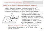
Geodesia. Cartografía. Sistemas de referencia. Tiempos.
Geodesia. Cartografía. Sistemas de referencia. Tiempos.
Geodesia. Cartografía. Sistemas de referencia. Tiempos.

Create successful ePaper yourself
Turn your PDF publications into a flip-book with our unique Google optimized e-Paper software.
<strong>Sistemas</strong> <strong>de</strong> navegación integrados<br />
Filtrado óptimo <strong>de</strong> sistemas lineales: el filtro <strong>de</strong> Kalman.<br />
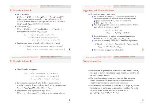
El filtro <strong>de</strong> Kalman II<br />
Deducción <strong>de</strong>l filtro <strong>de</strong> Kalman. Ecuaciones.<br />
Ejemplo <strong>de</strong> un filtro <strong>de</strong> Kalman<br />
En la ecuación<br />
ˆx + (tk+1) = ˆx − (tk+1) + Kk+1(z(tk+1) − Hk+1ˆx − (tk+1)) lo<br />
único que no conocemos es Kk+1, que es la ganancia <strong>de</strong><br />
Kalman. Ésta se <strong>de</strong>termina para garantizar que la covarianza<br />
, sea la menor posible.<br />
<strong>de</strong> ˆx + (tk+1), P +<br />
k+1<br />
Calculemos P +<br />
k+1 :<br />
P +<br />
k+1 = E[(x(tk+1) − ˆx + (tk+1))(x(tk+1) − ˆx + (tk+1)) T ], y<br />
sustituyendo la ecuación <strong>de</strong> ˆx + (tk+1):<br />
P + k+1<br />
" „<br />
= E x(tk+1 ) − ˆx + « „<br />
(tk+1 ) x(tk+1 ) − ˆx + « #<br />
T<br />
(tk+1 )<br />
»„<br />
= E x(tk+1 ) − ˆx − (tk+1 ) − Kk+1 (z(tk+1 ) − Hk+1 ˆx − «<br />
(tk+1 )<br />
„<br />
× x(tk+1 ) − ˆx − (tk+1 ) − Kk+1 (z(tk+1 ) − Hk+1 ˆx − « #<br />
T<br />
(tk+1 ))<br />
Sustituyendo ahora z(tk+1) = Hk+1x(tk+1) + ν(tk+1):<br />
P +<br />
k+1 =<br />
h“<br />
E x(tk+1) − ˆx − (tk+1) − Kk+1(Hk+1x(tk+1) + ν(tk+1) − Hk+1ˆx − ”<br />
(tk+1) “<br />
× x(tk+1) − ˆx − (tk+1) − Kk+1(Hk+1x(tk+1) + ν(tk+1) − Hk+1ˆx − ” –<br />
T<br />
(tk+1)) <strong>Sistemas</strong> <strong>de</strong> navegación integrados<br />
Filtrado óptimo <strong>de</strong> sistemas lineales: el filtro <strong>de</strong> Kalman.<br />
El filtro <strong>de</strong> Kalman III<br />
Simplificando, obtenemos:<br />
Deducción <strong>de</strong>l filtro <strong>de</strong> Kalman. Ecuaciones.<br />
Ejemplo <strong>de</strong> un filtro <strong>de</strong> Kalman<br />
P +<br />
k+1 =<br />
h“<br />
E (I − Kk+1Hk+1)(x(tk+1) − ˆx − ”<br />
) − Kk+1ν(tk+1) “<br />
× (I − Kk+1Hk+1)(x(tk+1) − ˆx − ” –<br />
T<br />
) − Kk+1ν(tk+1) = (I − K k+1H k+1)P −<br />
k+1 (I − K k+1H k+1) T + K k+1R k+1K T<br />
k+1<br />
Es necesario encontrar el valor <strong>de</strong> Kk+1 que minimiza la<br />
anterior expresión. Usando cálculo matricial, se encuentra que<br />
Kk+1 = P −<br />
k+1HT <br />
k+1<br />
Hk+1P −<br />
k+1HT −1 k+1 + Rk+1<br />
Sustituyendo ésta expresión se llega a que:<br />
P +<br />
−<br />
k+1 = (I − Kk+1Hk+1)Pk+1 . Ésta es la covarianza mínima.<br />
13 / 26<br />
14 / 26<br />
<strong>Sistemas</strong> <strong>de</strong> navegación integrados<br />
Filtrado óptimo <strong>de</strong> sistemas lineales: el filtro <strong>de</strong> Kalman.<br />
Algoritmo <strong>de</strong>l filtro <strong>de</strong> Kalman<br />
Deducción <strong>de</strong>l filtro <strong>de</strong> Kalman. Ecuaciones.<br />
Ejemplo <strong>de</strong> un filtro <strong>de</strong> Kalman<br />
El algoritmo queda como sigue:<br />
1 En el instante <strong>de</strong> tiempo tk+1, suponemos que tenemos la<br />
anterior estimación que incluyó también la última medida:<br />
ˆx + (tk) y su covarianza P + tk. Para k = 0 tomamos<br />
ˆx + (t0) = ˆx 0 y P + 0<br />
= P0.<br />
2 Fase <strong>de</strong> propagación; usamos la ecuación <strong>de</strong>l sistema dinámico<br />
para calcular la estimación a priori:<br />
ˆx − (tk+1) = Ak ˆx + (tk),<br />
P −<br />
k+1<br />
= AkP +<br />
k AT k + BkQkB T k .<br />
3 Preparándonos para la medida, calculamos la ganacia <strong>de</strong><br />
Kalman: Kk+1 = P −<br />
k+1HT <br />
k+1<br />
Hk+1P −<br />
k+1HT −1. k+1 + Rk+1<br />
4 Tomamos la medida y calculamos la estimación a posteriori:<br />
ˆx + (tk+1) = ˆx − (tk+1) + Kk+1(z(tk+1) − Hk+1ˆx − (tk+1)),<br />
P +<br />
k+1<br />
= (I − Kk+1Hk+1)P −<br />
k+1 .<br />
5 Iteramos para los siguientes valores <strong>de</strong> k.<br />
<strong>Sistemas</strong> <strong>de</strong> navegación integrados<br />
Filtrado óptimo <strong>de</strong> sistemas lineales: el filtro <strong>de</strong> Kalman.<br />
Sobre las medidas<br />
Deducción <strong>de</strong>l filtro <strong>de</strong> Kalman. Ecuaciones.<br />
Ejemplo <strong>de</strong> un filtro <strong>de</strong> Kalman<br />
Observación: es posible que no se realice una medida cada tk,<br />
sino que en ciertos instantes se hagan medidas, y en otros no<br />
se haga ninguna medida.<br />
Por ejemplo po<strong>de</strong>mos tener un sensor con bajo ancho <strong>de</strong><br />
banda (como el GPS) mientras que nuestro tiempo <strong>de</strong><br />
muestreo ∆t representa una elevada frecuencia.<br />
Una forma <strong>de</strong> solucionarlo es tomar Hk = 0, luego Kk = 0 en<br />
los instantes tk en los que no se realizan medidas. Por tanto<br />
no es necesario realizar ninguna actualización y<br />
ˆx + (tk) = ˆx − (tk), P + (tk) = P − (tk).<br />
15 / 26<br />
16 / 26