difracción de rayos x - Facultad de Ingeniería - UBA - Universidad ...
difracción de rayos x - Facultad de Ingeniería - UBA - Universidad ...
difracción de rayos x - Facultad de Ingeniería - UBA - Universidad ...

You also want an ePaper? Increase the reach of your titles
YUMPU automatically turns print PDFs into web optimized ePapers that Google loves.
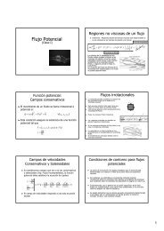
n<br />
n´<br />
d cosθ =d.n<br />
Θ<br />
Física <strong>de</strong>l Estado Sólido<br />
k k<br />
d<br />
Θ<br />
d cos θ ´ = −d.n´<br />
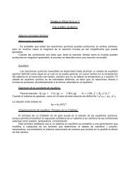
DIFRACCIÓN DE RAYOS X<br />
k´<br />
k´<br />
<strong>Facultad</strong> <strong>de</strong> <strong>Ingeniería</strong><br />
<strong>Universidad</strong> <strong>de</strong> Buenos Aires<br />
2009<br />
Dr. Andrés Ozols
TEMARIO<br />
• Objetivo<br />
• Naturaleza <strong>de</strong> los <strong>rayos</strong> X<br />
• Generación <strong>de</strong> los <strong>rayos</strong> X<br />
• Interacción con la materia<br />
• Difracción <strong>de</strong> <strong>rayos</strong> X<br />
• Equipo experimental<br />
• Factor <strong>de</strong> estructura y funciones <strong>de</strong> distribución<br />
• Estructura <strong>de</strong> los materiales: or<strong>de</strong>n <strong>de</strong> corto rango, <strong>de</strong><br />
rango intermedio y <strong>de</strong> largo rango
OBJETIVO<br />
Determinación <strong>de</strong> la Estructura Cristalina por<br />
Difracción <strong>de</strong> Rayos X<br />
Longitud <strong>de</strong> onda ≈ distancia inter-atómica<br />
inter atómica
NATURALEZA DE LOS RAYOS X<br />
0.5 - 5 Å
Tubo <strong>de</strong> GENERACIÓN RAYOS X<br />
Agua <strong>de</strong> refrigeración<br />
Anticá todo<br />
Fe, Mo, Cu<br />
Ra yos X<br />
Ha z <strong>de</strong><br />
Ele c trone s<br />
Ra yos X<br />
- Filamento<br />
Colimador <strong>de</strong> haz<br />
Ventana <strong>de</strong> Berilio
EQUIPO <strong>de</strong> DIFRACCIÓN <strong>de</strong> RAYOS X
DIFRACTOMETRO <strong>de</strong> RAYOS X<br />
Goniómetro tipo ”Θ−Θ”<br />
Radiación Molib<strong>de</strong>no ( línea Kα )
GENERACIÓN RAYOS X<br />
Energía cinética<br />
<strong>de</strong> los electrones<br />
Disipación <strong>de</strong> energía<br />
CALOR<br />
en el frenado<br />
Ec = e V<br />
10-50 KeV<br />
los electrones<br />
frenados generan<br />
E0<br />
Ef<br />
transiciones electrónicas<br />
e-<br />
en los átomos<br />
h ν<br />
RAYOS X
Intensidad <strong>de</strong> la radiación<br />
ESPECTRO DE RAYOS X<br />
Espectro continuo Espectro característico<br />
Longitud <strong>de</strong> onda<br />
Es función <strong>de</strong>l potencial V<br />
+<br />
Cuando este supera un valor Vc<br />
(<strong>de</strong>pendiente <strong>de</strong>l material) aparece<br />
el espectro característico<br />
Intensidad <strong>de</strong> la radiación<br />
K β<br />
K α<br />
Longitud <strong>de</strong> onda<br />
líneas <strong>de</strong> series K, L, M, N
ESPECTRO DE RAYOS X<br />
Intensidad <strong>de</strong> la radiación<br />
K β<br />
K α<br />
Longitud <strong>de</strong> onda
LONGITUDES DE ONDA CARACTERÍSTICAS<br />
Elemento<br />
Ca<br />
Ti<br />
V<br />
Cr<br />
Mn<br />
Fe<br />
Co<br />
Ni<br />
Cu<br />
Zn<br />
λ α<br />
3.357<br />
2.766<br />
2.521<br />
2.295<br />
2.117<br />
1.945<br />
1.796<br />
1.664<br />
1.548<br />
1.448<br />
λ β<br />
3.085<br />
2.528<br />
2.302<br />
2.088<br />
1.923<br />
1.765<br />
1.635<br />
1.504<br />
1.403<br />
-
Intensidad <strong>de</strong> la radiación<br />
FILTRADO <strong>de</strong> Líneas <strong>de</strong> RAYOS X<br />
Radiación XK α K β ,<br />
K α<br />
Longitud <strong>de</strong> onda<br />
Línea K α filtrada<br />
Intensidad <strong>de</strong> la radiación<br />
Filtros + monocromador<br />
K β<br />
K α<br />
Co<br />
Longitud <strong>de</strong> onda<br />
Radiación<br />
Cu<br />
Mo<br />
Filtro<br />
Ni<br />
Zr<br />
Fe
d<br />
DIFRACCION <strong>de</strong> RAYOS X en CRISTALES<br />
dsenθ<br />
d 1<br />
θ<br />
θ<br />
d 2<br />
Familias <strong>de</strong> planos con separaciones d y d<br />
1 2<br />
∆caminos ópticos = 2d sin θ<br />
Si hay interferencia<br />
constructiva<br />
Ley <strong>de</strong> Bragg<br />
2d sin θ = λ<br />
cada familia (d, d 1, d 2)<br />
<strong>de</strong> planos tiene un<br />
ángulo θ que satisface<br />
esta ley
DIFRACTOGRAMAS <strong>de</strong> RAYOS X<br />
Intensidad<br />
100<br />
80<br />
60<br />
40<br />
20<br />
0<br />
Si O Cuarzo policristalino (en polvo)<br />
2<br />
Radiación Kα <strong>de</strong>l Cu<br />
20 30 40 50 60 70 80 90<br />
2 θ
POSICIONES <strong>de</strong> las REFLEXIONES en DISTINTOS PLANOS
IDENTIFICACION <strong>de</strong> COMPUESTOS Base <strong>de</strong> compuestos inorgánicos<br />
y orgánicos)<br />
Tarjeta <strong>de</strong>l Joint Committee of Pow<strong>de</strong>r Diffraction Files (JCPDF)
TARJETA <strong>de</strong> IDENTIFICACIÓN <strong>de</strong> COMPUESTO<br />
Joint Committee of Pow<strong>de</strong>r Diffraction Files (JCPDF)
APLICACIONES <strong>de</strong> la DIFRACCION <strong>de</strong> RAYOS X<br />
La <strong>difracción</strong> <strong>de</strong> <strong>rayos</strong> X es una técnica versátil,<br />
no-<strong>de</strong>structiva y analítica para la <strong>de</strong>terminación<br />
<strong>de</strong>:<br />
•Fases<br />
•Estructura<br />
•Textura<br />
•Tensiones<br />
Que pudieran estar presentes en materiales<br />
sólidos, polvos, y líquidos
APLICACIONES a MATERIA CONDENSADA
Temario<br />
•Bases <strong>de</strong> la teoría <strong>de</strong> <strong>difracción</strong> <strong>de</strong> <strong>rayos</strong> X<br />
•Aplicación <strong>de</strong> la teoría <strong>de</strong> <strong>difracción</strong> <strong>de</strong> <strong>rayos</strong> X<br />
•Aberraciones geométricas<br />
•Tamaño <strong>de</strong> cristalito<br />
•Imperfecciones <strong>de</strong> la red<br />
•Medidas <strong>de</strong>l ancho <strong>de</strong> línea<br />
•Formulación <strong>de</strong> Von Laue <strong>de</strong> la <strong>difracción</strong> <strong>de</strong> <strong>rayos</strong> x por un<br />
cristal<br />
•Equivalencia <strong>de</strong> las formulaciones <strong>de</strong> Bragg y Von Laue<br />
•Difracción por una red con una base monatómica<br />
•Factor <strong>de</strong> estructura geométrico<br />
•Difracción por un cristal poliatómico<br />
•El factor atómico <strong>de</strong> forma
INTENSIDAD I(θ) DISPERSADA<br />
( θ )<br />
I = I<br />
( )<br />
( )<br />
( )<br />
( )<br />
2 2 2<br />
1 1 2 2 3 3<br />
0 2<br />
sen 1<br />
2<br />
sen 2<br />
2<br />
sen 3<br />
( )<br />
( )<br />
sen ⎡⎣Nψθ, λ ⎤⎦ sen ⎡⎣N ψ θ, λ ⎤⎦ sen ⎡⎣Nψ θ, λ ⎤⎦<br />
⎡⎣ ψ θ, λ ⎤⎦ ⎡⎣ψ θ, λ ⎤⎦ ⎡⎣ψ θ, λ ⎤⎦<br />
•1,2 y 3 a las direcciones <strong>de</strong> vectores base <strong>de</strong> la red <strong>de</strong> Bravais<br />
•θ es la mitad <strong>de</strong>l ángulo <strong>de</strong> dispersión, entre direcciones <strong>de</strong> los haces<br />
inci<strong>de</strong>nte y el dispersado.<br />
•λ es la longitud <strong>de</strong> onda <strong>de</strong>l haz <strong>de</strong> <strong>rayos</strong> X inci<strong>de</strong>nte.<br />
•Nl , N2 y N3 representan la cantidad total <strong>de</strong> nodos en cada direcciones
Difractograma característico<br />
(intensidad relativa en función <strong>de</strong> 2θ).<br />
Intensidad<br />
100<br />
80<br />
60<br />
40<br />
20<br />
0<br />
Si O Cuarzo policristalino (en polvo)<br />
2<br />
Radiación Kα <strong>de</strong>l Cu<br />
20 30 40 50 60 70 80 90<br />
2 θ
INTENSIDAD I(θ) DISPERSADA<br />
f<br />
( θ )<br />
=<br />
( )<br />
( )<br />
sen ⎡⎣Nψθ⎤⎦ sen ⎡⎣ψ θ ⎤⎦<br />
máximos <strong>de</strong> intensidad están dados por la ley <strong>de</strong> Bragg<br />
2dhklsenθ= nλ<br />
d hkl es la distancia o espaciado reticular<br />
<strong>de</strong> familia <strong>de</strong> planos (h k l)<br />
n = 1,2,3,... es or<strong>de</strong>n <strong>de</strong> la <strong>difracción</strong><br />
d<br />
dsenθ<br />
d 1<br />
θ<br />
θ<br />
d 2<br />
Familias <strong>de</strong> planos con separaciones d y d<br />
1 2
Aplicación <strong>de</strong> la teoría <strong>de</strong> <strong>difracción</strong> <strong>de</strong> <strong>rayos</strong> X<br />
i) Aberraciones geométricas<br />
Función <strong>de</strong> las características <strong>de</strong>l equipo <strong>de</strong><br />
<strong>difracción</strong> y los parámetros <strong>de</strong> control <strong>de</strong>l<br />
goniómetro:<br />
•Rango <strong>de</strong> barrido 2θ 0 -2θ f <strong>de</strong> barrido (2-100º)<br />
•Velocidad <strong>de</strong> barrido 2θ/min (0.1-2º/min)<br />
•Resolución angular o paso (0.01-1º)<br />
•Tensión <strong>de</strong> la fuente (20-60 KV)<br />
•Corriente <strong>de</strong> filamento<br />
•Combinación <strong>de</strong> rendijas para colimación y<br />
filtrado <strong>de</strong> RX<br />
Goniómetro tipo ”θ−θ”
CONFIGURACION <strong>de</strong>l EQUIPO <strong>de</strong> DIFRACCIÓN <strong>de</strong> RAYOS X
ii) Tamaño <strong>de</strong> cristalito<br />
Estructura policristalina<br />
granos<br />
granos con<br />
orientaciones<br />
cristalográficas<br />
diferentes
iii) Imperfecciones <strong>de</strong> la red<br />
Macla<br />
Dislocación <strong>de</strong> bor<strong>de</strong><br />
Dislocación helicoidal
I p<br />
Medidas <strong>de</strong>l ancho <strong>de</strong> línea<br />
( )<br />
I( 2θ2) − I(<br />
2θ1)<br />
Semi-ancho<br />
2θ 3<br />
AREA<br />
B 1/2<br />
AREA<br />
2θ 4<br />
B<br />
1/2<br />
=<br />
2<br />
1<br />
Bi= I d<br />
I ∫<br />
P<br />
( 2θ) ( 2θ)<br />
I p<br />
I/2<br />
p<br />
2θ 1<br />
B 1/2<br />
Ancho integral Bi<br />
I p Varianza o <strong>de</strong>sviación cuadrática Standard<br />
W<br />
2θ<br />
= ∫<br />
2<br />
( 2θ−2θ ) I( 2θ) d(<br />
2θ)<br />
∫<br />
I( 2θ) d(<br />
2θ)<br />
2θ 2
n<br />
FORMULACIÓN <strong>de</strong> VON LAUE <strong>de</strong> la DIFRACCIÓN<br />
n´<br />
d cosθ =d.n<br />
Θ<br />
k k<br />
d<br />
Θ<br />
d cos θ ´ = −d.n´<br />
k´<br />
k´<br />
Diferencia <strong>de</strong> caminos <strong>de</strong> los <strong>rayos</strong><br />
dispersados<br />
<br />
dcosθ + dcos θ´<br />
= d. n−n´ ( ˆ ˆ )<br />
interferencia constructiva ⇔<br />
<br />
d. n− n´ = mλ<br />
( ˆ ˆ )<br />
Multiplicando x 2π/λ<br />
<br />
d. k − k´ = 2πm<br />
( )<br />
<br />
<br />
R. k − k´ = 2πm<br />
d = R es vector <strong>de</strong> la red <strong>de</strong> Bravais ⇒ ( )
FORMULACIÓN <strong>de</strong> VON LAUE <strong>de</strong> la DIFRACCIÓN<br />
<br />
R. k − k´ = 2πm<br />
K/2<br />
k<br />
( )<br />
plano <strong>de</strong> Bragg<br />
k´<br />
R ∈ red <strong>de</strong> Bravais<br />
K ∈ red <strong>de</strong> Recíproca<br />
K/2<br />
k = K − k<br />
<br />
e<br />
i( k´ −k).<br />
R<br />
<br />
iK. R<br />
e =<br />
1<br />
= 1<br />
condición <strong>de</strong> Laue<br />
K= k´-k<br />
<br />
K <br />
ˆ 1<br />
k. = k. K = K<br />
K 2
EQUIVALENCIA <strong>de</strong> las FORMULACIONES <strong>de</strong> BRAGG y VON LAUE<br />
<br />
K = k´ −k<br />
∈ red <strong>de</strong> Recíproca<br />
k y k´ con el mismo θ y perpendicular al<br />
plano <strong>de</strong> K<br />
K = n K 0<br />
K<br />
K 0 vector <strong>de</strong> la red recíproca <strong>de</strong><br />
longitud mínima = 2π/d<br />
=<br />
2π n<br />
d<br />
k<br />
K= k´ -k<br />
θ<br />
K = 2k senθ<br />
2d senθ = nλ<br />
k senθ<br />
k senθ<br />
θ<br />
-k<br />
θ<br />
θ<br />
k´<br />
k = 2π/λ<br />
reflexión <strong>de</strong> Bragg
DIFRACCIÓN por una RED con una BASE MONATÓMICA<br />
Red <strong>de</strong> Bravais<br />
+<br />
n- átomos <strong>de</strong> una base<br />
d 1 d2 d 3<br />
d 4<br />
d 5<br />
=<br />
cristal
FACTOR <strong>de</strong> ESTRUCTURA GEOMÉTRICO<br />
<br />
K = k´ −k<br />
pico <strong>de</strong> Bragg<br />
<br />
K.( di − d j)<br />
d j<br />
d i<br />
e<br />
<br />
iK .( d −d<br />
)<br />
i j<br />
amplitu<strong>de</strong>s <strong>de</strong> los <strong>rayos</strong> dispersados en d1,.., d iK. d<br />
n, 1<br />
Amplitud total ∝<br />
<br />
K<br />
n<br />
iK. d<br />
= ∑<br />
j=<br />
1<br />
<br />
S e<br />
j<br />
diferencia <strong>de</strong> la fase<br />
diferencia <strong>de</strong><br />
amplitu<strong>de</strong>s<br />
e <br />
I ∝<br />
Intensidad total<br />
e<br />
<br />
iK . dn<br />
S <br />
K<br />
2
DISPERSION por un ATOMO<br />
λ∝dimensiones atómicas<br />
+<br />
CB-AD diferencia <strong>de</strong><br />
camino <strong>de</strong> Z´ repecto Z<br />
interferencia<br />
<strong>de</strong>structiva<br />
Factor <strong>de</strong> dispersión o<br />
forma atómica<br />
Dispersión incoherente<br />
Dispersión coherente
DIFRACCIÓN por un CRISTAL POLIATÓMICO<br />
<br />
S = ∑ f K e<br />
n<br />
Si iones <strong>de</strong> base ≠ <br />
K<br />
j ( )<br />
f j factor <strong>de</strong> forma o dispersión atómico<br />
Depen<strong>de</strong> <strong>de</strong> la estructura <strong>de</strong>l ión<br />
número <strong>de</strong> electrones que ro<strong>de</strong>an un átomo<br />
j=<br />
1<br />
<br />
iK. d<br />
j<br />
<br />
( )<br />
1 <br />
iK . r <br />
f j K =− e ρ j(<br />
r) dr<br />
e ∫<br />
ρ j distribución <strong>de</strong> carga electrónica <strong>de</strong>l ión<br />
0<br />
( )<br />
∞<br />
sen kr<br />
f0 = ∫ ρ ( r) dr<br />
kr