1 Calcular ∫ Sec(θ)dθ tenemos que ∫ Sec(θ)dθ = ∫ Sec(θ)( Sec(θ ...
1 Calcular ∫ Sec(θ)dθ tenemos que ∫ Sec(θ)dθ = ∫ Sec(θ)( Sec(θ ...
1 Calcular ∫ Sec(θ)dθ tenemos que ∫ Sec(θ)dθ = ∫ Sec(θ)( Sec(θ ...

You also want an ePaper? Increase the reach of your titles
YUMPU automatically turns print PDFs into web optimized ePapers that Google loves.
<strong>Calcular</strong> <strong>Sec</strong>(<strong>θ</strong>)d<strong>θ</strong><br />
<strong>tenemos</strong> <strong>que</strong><br />
<br />
<br />
<strong>Sec</strong>(<strong>θ</strong>) + T an(<strong>θ</strong>)<br />
<strong>Sec</strong>(<strong>θ</strong>)d<strong>θ</strong> = <strong>Sec</strong>(<strong>θ</strong>)( )d<strong>θ</strong> =<br />
<strong>Sec</strong>(<strong>θ</strong>) + T an(<strong>θ</strong>)<br />
=<br />
du<br />
u<br />
<strong>Calcular</strong> ahora <strong>Sec</strong>3 (<strong>θ</strong>)d<strong>θ</strong><br />
<strong>tenemos</strong> <strong>que</strong><br />
<br />
<strong>Sec</strong> 3 <br />
(<strong>θ</strong>)d<strong>θ</strong> = <strong>Sec</strong> 2 (<strong>θ</strong>)<br />
<br />
<br />
= <strong>Sec</strong>(<strong>θ</strong>)T an(<strong>θ</strong>)−<br />
= Ln(u) + k = Ln(<strong>Sec</strong>(<strong>θ</strong>) + T an(<strong>θ</strong>)) + k<br />
dv=<strong>Sec</strong> 2 (<strong>θ</strong>)<br />
v=T an(<strong>θ</strong>)<br />
<strong>Sec</strong>(<strong>θ</strong>)<br />
<br />
u=<strong>Sec</strong>(<strong>θ</strong>)<br />
du=<strong>Sec</strong>(<strong>θ</strong>)T an(<strong>θ</strong>)<br />
d<strong>θ</strong> = <strong>Sec</strong>(<strong>θ</strong>)T an(<strong>θ</strong>)<br />
<strong>Sec</strong>2 (<strong>θ</strong>) + <strong>Sec</strong>(<strong>θ</strong>)T an(<strong>θ</strong>)<br />
<strong>Sec</strong>(<strong>θ</strong>) + T an(<strong>θ</strong>)<br />
<br />
u=<strong>Sec</strong>(<strong>θ</strong>)+T an(<strong>θ</strong>) du=<strong>Sec</strong>(<strong>θ</strong>)T an(<strong>θ</strong>)+<strong>Sec</strong>2 d<strong>θ</strong><br />
(<strong>θ</strong>)<br />
<br />
u∗v<br />
T an 2 <br />
(<strong>θ</strong>)<strong>Sec</strong>(<strong>θ</strong>)d<strong>θ</strong> = <strong>Sec</strong>(<strong>θ</strong>)T an(<strong>θ</strong>)−<br />
<br />
<strong>Sec</strong>(<strong>θ</strong>)T an(<strong>θ</strong>) −<br />
Por lo tanto<br />
<br />
<strong>Sec</strong> 3 <br />
(<strong>θ</strong>)d<strong>θ</strong> = <strong>Sec</strong>(<strong>θ</strong>)T an(<strong>θ</strong>) −<br />
simplificando<br />
<br />
2 <strong>Sec</strong> 3 <br />
(<strong>θ</strong>)d<strong>θ</strong> = <strong>Sec</strong>(<strong>θ</strong>)T an(<strong>θ</strong>)+<br />
<strong>Sec</strong> 3 <br />
(<strong>θ</strong>)d<strong>θ</strong> +<br />
<strong>Sec</strong>(<strong>θ</strong>)d<strong>θ</strong><br />
<strong>Sec</strong> 3 <br />
(<strong>θ</strong>)d<strong>θ</strong> +<br />
<br />
−<br />
1<br />
T an(<strong>θ</strong>)<strong>Sec</strong>(<strong>θ</strong>)T an(<strong>θ</strong>) d<strong>θ</strong><br />
<br />
− v∗du<br />
(<strong>Sec</strong> 2 −1)<strong>Sec</strong>(<strong>θ</strong>)d<strong>θ</strong> =<br />
<strong>Sec</strong>(<strong>θ</strong>)d<strong>θ</strong><br />
<strong>Sec</strong>(<strong>θ</strong>)d<strong>θ</strong> = <strong>Sec</strong>(<strong>θ</strong>)T an(<strong>θ</strong>)+Ln(<strong>Sec</strong>(<strong>θ</strong>)+T an(<strong>θ</strong>))<br />
finalmente nos <strong>que</strong>da<br />
<br />
<strong>Sec</strong> 3 (<strong>θ</strong>)d<strong>θ</strong> = 1<br />
(<strong>Sec</strong>(<strong>θ</strong>)T an(<strong>θ</strong>) + Ln(<strong>Sec</strong>(<strong>θ</strong>) + T an(<strong>θ</strong>)))<br />
2<br />
Calculemos √ x2 − 1dx haciendo el cambio de variable x = <strong>Sec</strong>(<strong>θ</strong>) Tenemos<br />
<strong>que</strong><br />
<br />
√x<br />
<br />
<strong>Sec</strong><br />
<br />
T<br />
2 − 1dx =<br />
2 (<strong>θ</strong>) − 1<strong>Sec</strong><strong>θ</strong>T an(<strong>θ</strong>)d<strong>θ</strong> = an2 (<strong>θ</strong>)<strong>Sec</strong>(<strong>θ</strong>)T an(<strong>θ</strong>)d<strong>θ</strong>
2<br />
<br />
<br />
= T an(<strong>θ</strong>)<strong>Sec</strong>(<strong>θ</strong>)T an(<strong>θ</strong>)d<strong>θ</strong> = T an 2 <br />
(<strong>θ</strong>)<strong>Sec</strong>(<strong>θ</strong>)d<strong>θ</strong> = (<strong>Sec</strong> 2 (<strong>θ</strong>)−1)<strong>Sec</strong>(<strong>θ</strong>)d<strong>θ</strong><br />
<br />
=<br />
<strong>Sec</strong> 3 (<strong>θ</strong>)−<strong>Sec</strong>(<strong>θ</strong>)d<strong>θ</strong> = 1<br />
<strong>Sec</strong>(<strong>θ</strong>)T an(<strong>θ</strong>)+1 Log(<strong>Sec</strong>(<strong>θ</strong>)+T an(<strong>θ</strong>))−Log(<strong>Sec</strong>(<strong>θ</strong>)+T an(<strong>θ</strong>))<br />
2 2<br />
= 1<br />
1<br />
1<br />
<strong>Sec</strong>(<strong>θ</strong>)T an(<strong>θ</strong>)− Log(<strong>Sec</strong>(<strong>θ</strong>)+T an(<strong>θ</strong>)) =<br />
2 2 2 (x√x2 − 1)− 1<br />
2 (x+√x2 − 1)<br />
En la hipérbola equilatera x 2 − y 2 = 1 definimos c = Cosh(x) s = Senh(x)<br />
y como c,s estan sobre la hipérbola c 2 − s 2 = 1<br />
c √ √ √<br />
Area = ”x” = sc − 2 x2 − 1dx = sc − c c2 − 1 + Log(c + c2 − 1)<br />
Por lo tanto<br />
1<br />
= sc − cs + Log(c + √ c 2 − 1) = Log(c + √ c 2 − 1)<br />
x = Log(c+ √ c 2 − 1) ⇒ e x = c+ √ c 2 − 1 ⇒ e x −c = √ c 2 − 1 ⇒ e 2x −2e x c+c 2 = c 2 −1<br />
⇒ e 2x − 2e x c = −1 ⇒ e 2x + 1 = 2e x c ⇒ e2x + 1<br />
2e x<br />
= c ⇒ c = ex + e −x<br />
De la relación c2 − s2 = 1 podemos obtener el valor de s<br />
s = √ c2 <br />
− 1 = ( ex + e−x )<br />
2<br />
2 <br />
e2x + 2 + e−2x e2x + 2 + e−2x − 4<br />
− 1 =<br />
− 1 =<br />
4<br />
4<br />
<br />
(ex − e−x ) 2<br />
=<br />
=<br />
4<br />
ex − e−x 2<br />
Tenemos <strong>que</strong><br />
2
por semejanza de triángulos t<br />
1<br />
= s<br />
c<br />
t = s<br />
c =<br />
⇒ t = s<br />
C<br />
e x −e −x<br />
2<br />
e x +e −x<br />
2<br />
finalmente definimos c = Cosh(x) = ex +e −x<br />
2<br />
por lo tanto<br />
= ex − e −x<br />
e x + e −x<br />
T anh(x) = ex −e −x<br />
e x +e −x<br />
Algunas propiedades de las funciones hipérbolicas<br />
Cosh 2 (x)−Senh 2 (x) = ( ex + e −x<br />
2<br />
, s = Senh(x) = ex −e −x<br />
2<br />
3<br />
y t =<br />
) 2 −( ex − e−x )<br />
2<br />
2 = e2x + 2 + e−2x − e2x + 2 − e−2x 4<br />
Cosh 2 (ArcSennh(x))−Senh 2 (ArcSennh(x)) = 1 ⇒ Cosh(ArcSennh(x)) = √ 1 + x 2<br />
Cosh 2 (ArcSennh(x))−Senh 2 (ArcSennh(x)) = 1 ⇒ Senh(ArcSennh(x)) = √ x 2 − 1<br />
(ArcCosh(x)) ′ =<br />
Por lo tanto <br />
Otro camino<br />
<br />
<br />
1<br />
√ dx =<br />
x2 − 1<br />
<br />
x=Cosh(t)<br />
dx=Senh(x)<br />
1<br />
Cosh ′ (ArcCosh(x)) =<br />
1<br />
√ x 2 − 1 = ArcCosh(x)<br />
Senh(t)<br />
Cosh 2 (t) − 1 dt =<br />
1<br />
Senh(ArcCosh(x)) =<br />
<br />
Senh(t)<br />
dt =<br />
Senh(t)<br />
1<br />
√ x 2 − 1<br />
dt = t = ArcCosh(x)<br />
= 4<br />
4<br />
= 1
4<br />
Funciones Elipticas<br />
<br />
Mediante un análisis similar pero de la elipse se obtienen integrales<br />
dx<br />
,<br />
(1 − x2 )(1 − k2x2 )<br />
<br />
x2dx ,<br />
(1 − x2 )(1 − k2x2 )<br />
<br />
dx<br />
(x − a) (1 − x2 )(1 − k2x2 )<br />
<strong>que</strong> son llamadas integrales elipticas, como x necesariamente tiene <strong>que</strong> ser<br />
menor <strong>que</strong> 1, pues de lo contrario la raíz se haría negativa, podemos hacer el<br />
cambio x = Sen(ϕ) por lo <strong>que</strong> nos <strong>que</strong>da<br />
<br />
dx<br />
(1 − x 2 )(1 − k 2 x 2 ) =<br />
<br />
dϕ<br />
(1 − k 2 Sen 2 (ϕ))<br />
Integral Eliptica de 1ra especie<br />
Se define al seno eliptico de Jacobi como la función inversa de la integral<br />
eliptica de primera especie.<br />
Consideremos la integral eliptica de primera especie<br />
z<br />
u = Fk(z) =<br />
0<br />
dz<br />
(1 − z 2 )(1 − k 2 z 2 )<br />
La inversa de esta función es la primera de tres funciones elipticas de Jacobi<br />
snu = x = F −1<br />
k (u)<br />
Las otras dos funciones elipticas de Jacobi se definen a partir de esta por las<br />
relaciones siguientes:<br />
cnu = 1 − sn 2 (u) = √ 1 − x 2 dnu = 1 − k 2 sn 2 (u) = √ 1 − k 2 x 2<br />
Las funciones elipticas de Jacobi son funciones definidas a partir de la integral<br />
eliptica de primera especie y aparecen en diversos contextos, deben su nombre<br />
al matemático aleman Carl Gustav Jakob Jacobi.<br />
En física aparecen por ejemplo en las osilaciones de un péndulo con<br />
grandes amplitudes sometido a la gravedad.<br />
Algunas propiedades de las funciones elíticas son:<br />
cn 2 (u) + sn 2 (u) = ( 1 − sn 2 (u)) 2 + x 2 = ( √ 1 − x 2 ) 2 + x 2 = 1<br />
dn 2 (u) + k 2 sn 2 (u) = ( √ 1 − k 2 x 2 ) 2 + k 2 x 2 = 1<br />
dn 2 − k 2 cn 2 (u) = ( √ 1 − k 2 x 2 ) 2 − k 2 ( √ 1 − x 2 ) 2 = 1 − k 2
Las funciones elípticas son una generalización de las funciones circulares e<br />
hipérbolicas. Cuando k=0 la integral elíptica se convierte en:<br />
<br />
<br />
dx<br />
dx<br />
= √ = ArcSen(x)<br />
(1 − x2 )(1 − k2x2 ) 1 − x2 cuando k=1<br />
<br />
<br />
dx<br />
=<br />
(1 − x2 )(1 − k2x2 )<br />
<br />
dx<br />
=<br />
(1 − x2 )(1 − x2 )<br />
dx<br />
1 − x 2<br />
la cual podemos resolver de la siguiente manera<br />
<br />
<br />
dx 1<br />
=<br />
1 − x2 2<br />
<br />
2dx 1 1 − x + 1 + xdx<br />
=<br />
1 − x2 2 1 − x2 = 1<br />
<br />
(1 − x)dx (1 + x)dx<br />
+1<br />
2 1 − x2 2 1 − x2 = 1<br />
<br />
2<br />
(1 − x)dx<br />
(1 − x)(1 + x) +1<br />
<br />
2<br />
<br />
(1 + x)dx 1<br />
=<br />
(1 + x)(1 − x) 2<br />
1dx<br />
1 + x +1<br />
<br />
2<br />
1dx 1<br />
=<br />
1 − x 2 Ln(1+x)−1<br />
2 Ln(1−x)+k<br />
= 1 + x<br />
Ln(1 ) + k<br />
2 1 − x<br />
5