Una demostración del Teorema de Wigner para matrices ... - Cimat
Una demostración del Teorema de Wigner para matrices ... - Cimat
Una demostración del Teorema de Wigner para matrices ... - Cimat

Create successful ePaper yourself
Turn your PDF publications into a flip-book with our unique Google optimized e-Paper software.
<strong>Una</strong> <strong><strong>de</strong>mostración</strong> <strong><strong>de</strong>l</strong> <strong>Teorema</strong> <strong>de</strong> <strong>Wigner</strong> <strong>para</strong><br />
<strong>matrices</strong> aleatorias<br />
Ana Marlene López Ramos<br />
Abril <strong>de</strong> 2011
Contenido<br />
Prefacio 3<br />
1 Preliminares 5<br />
1.1 Distribución<strong><strong>de</strong>l</strong>semicírculo ........................... 9<br />
1.2 Números <strong>de</strong> Catalan ............................... 9<br />
1.3 Gráficas ...................................... 11<br />
1.3.1 De la traza a las gráficascíclicas..................... 13<br />
1.3.2 Procedimiento<strong>de</strong>truncamiento ..................... 18<br />
1.3.3 Operaciones con aristas <strong>de</strong> una gráfica ................. 19<br />
1.3.4 Cotas superiores <strong>para</strong> ......................... 22<br />
2 El <strong>Teorema</strong> <strong>de</strong> <strong>Wigner</strong> 25<br />
2.1 Demostración<strong><strong>de</strong>l</strong><strong>Teorema</strong><strong>de</strong><strong>Wigner</strong>...................... 26<br />
2.1.1 Convergencia en esperanza <strong>de</strong> ¯ ................... 26<br />
2.1.2 Convergencia casi segura <strong>de</strong> ¯ .................... 30<br />
2.1.3 Com<strong>para</strong>ción <strong>de</strong> y ¯ ...................... 36<br />
2.1.4 Convergencia<strong><strong>de</strong>l</strong>aFDEEoriginal.................... 37<br />
3 Estudio <strong>de</strong> simulación 39<br />
3.1 Ejemplosbajolossupuestos<strong><strong>de</strong>l</strong><strong>Teorema</strong><strong>de</strong><strong>Wigner</strong>.............. 41<br />
3.2 Ejemplossinlossupuestos<strong><strong>de</strong>l</strong><strong>Teorema</strong><strong>de</strong><strong>Wigner</strong>............... 44<br />
A Demostraciones 47<br />
B Resultados <strong>de</strong> Probabilidad 59<br />
B.1 Tipos <strong>de</strong> convergencia .............................. 59<br />
B.1.1 Convergencia en probabilidad . . .................... 59<br />
B.1.2 Desigualdad<strong>de</strong>Chebyshev........................ 59<br />
B.1.3 Convergenciacasisegura......................... 60<br />
B.1.4 Convergenciaendistribuciónydébil .................. 60<br />
B.1.5 Lema<strong>de</strong>Borel-Cantelli.......................... 60<br />
B.2 Notación “O gran<strong>de</strong>”............................... 61<br />
Bibliografía 63<br />
1
CONTENIDO 2
Prefacio<br />
En esta tesis se presenta una <strong><strong>de</strong>mostración</strong> <strong><strong>de</strong>l</strong> <strong>Teorema</strong> <strong>de</strong> <strong>Wigner</strong> <strong>para</strong> <strong>matrices</strong> aleatorias<br />
simétricas reales. Este resultado juega un papel fundamental en la teoría <strong>de</strong> <strong>matrices</strong><br />
aleatorias, área que actualmente está siendo ampliamente investigada, ver [3], [7], [9].<br />
<strong>Una</strong> matriz <strong>de</strong> <strong>Wigner</strong> es una matriz aleatoria simétrica (o hermitiana en el caso complejo).<br />
Estas <strong>matrices</strong> juegan un papel importante en Física Nuclear y Física Matemática.<br />
Para aplicaciones en estas áreas ver el libro <strong>de</strong> Mehta (2004) [9].<br />
Sea una matriz aleatoria <strong>de</strong> dimensión × con eigenvalores , =12 Si es simétrica, estos eigenvalores son reales. En consecuencia, es posible <strong>de</strong>finir una<br />
función <strong>de</strong> distribución unidimensional<br />
1<br />
() =<br />
# { ≤ : ≤ } <br />
llamada la función <strong>de</strong> distribución espectral empírica (FDEE) <strong>de</strong> la matriz <br />
Uno <strong>de</strong> los principales problemas en Teoría <strong>de</strong> <strong>matrices</strong> aleatorias es investigar la convergencia<br />
<strong>de</strong> la sucesión <strong>de</strong> FDEE’s © <br />
ª<br />
<strong>para</strong> una sucesión <strong>de</strong> <strong>matrices</strong> aleatorias dada<br />
≥1<br />
{} ≥1 El límite <strong>de</strong> la FDEE <strong>de</strong> la sucesión {} si existe se llama distribución espectral<br />
asintótica .<br />
La investigación <strong><strong>de</strong>l</strong> límite <strong>de</strong> la FDEE <strong>de</strong> <strong>matrices</strong> aleatorias cuando →∞es <strong>de</strong><br />
gran interés entre físicos, matemáticos, probabilistas y estadísticos, entre otros. El interés en<br />
la FDEE radica en que muchas estadísticas importantes en análisis estadístico multivariado<br />
se pue<strong>de</strong>n expresar en términos <strong>de</strong> la FDEE. Un ejemplo es el siguiente.<br />
Sea una matriz <strong>de</strong>finida positiva <strong>de</strong> dimensión × . Tenemos que<br />
<strong>de</strong>t () = Q<br />
∙ Z ∞<br />
=exp<br />
(log ) ¸<br />
() <br />
=1<br />
don<strong>de</strong> es la FDEE <strong>de</strong> la matriz <br />
En particular en esta tesis, consi<strong>de</strong>raremos <strong>matrices</strong> <strong>de</strong> <strong>Wigner</strong> reales, i.e., <strong>matrices</strong><br />
aleatorias simétricas reales tales que = () don<strong>de</strong> las variables aleatorias son<br />
in<strong>de</strong>pendientes si 1 ≤ ≤ ≤ <br />
El objetivo principal <strong>de</strong> esta tesis es presentar una <strong><strong>de</strong>mostración</strong> <strong>de</strong>tallada <strong><strong>de</strong>l</strong> <strong>Teorema</strong><br />
<strong>de</strong> <strong>Wigner</strong>, el cual establece que bajo ciertas condiciones sobre ,<br />
()<br />
<br />
−→ () ∀ ∈ R<br />
→∞<br />
don<strong>de</strong> () es la función <strong>de</strong> distribución <strong><strong>de</strong>l</strong> semicírculo cuya función <strong>de</strong> <strong>de</strong>nsidad está dada<br />
() cuya expresión explícita se<br />
por () = 1<br />
√ R<br />
4 − 2 <br />
−2 ≤ ≤ 2 i.e., () = 2<br />
−∞<br />
3<br />
0
CONTENIDO 4<br />
pue<strong>de</strong> ver en la Sección 1, usando herramienta <strong>de</strong> teoría <strong>de</strong> gráficas, combinatoria y técnicas<br />
<strong>de</strong> probabilidad relacionadas con los métodos <strong>de</strong> momentos y truncamiento, así como el<br />
uso <strong>de</strong> la <strong>de</strong>sigualdad <strong>de</strong> Chebyshev y el Lema <strong>de</strong> Borel-Cantelli. Se utiliza el método <strong><strong>de</strong>l</strong><br />
truncamiento<strong>de</strong>bidoaquelapruebaserealizarápidiendoquelascomponentes<strong><strong>de</strong>l</strong>amatriz<br />
aleatoria tengan un <strong>de</strong>terminado número <strong>de</strong> momentos finitos.<br />
Como segundo objetivo <strong>de</strong> esta tesis es ilustrar la vali<strong>de</strong>z <strong><strong>de</strong>l</strong> <strong>Teorema</strong> <strong>de</strong> <strong>Wigner</strong> <strong>para</strong><br />
<strong>matrices</strong> aleatorias mediante un estudio <strong>de</strong> simulación.<br />
En 1958 <strong>Wigner</strong> [12] da una <strong><strong>de</strong>mostración</strong> heurística <strong><strong>de</strong>l</strong> teorema solicitando una matriz<br />
<strong>de</strong> dimensión con entradas reales, simétrica, don<strong>de</strong> las variables aleatorias son in<strong>de</strong>pendientes<br />
<strong>para</strong> 1 ≤ ≤ ≤ , todos los momentos <strong>de</strong> los existen y el segundo momento<br />
<strong>de</strong> todos las es el mismo.<br />
Arnold [2] <strong>de</strong>muestra el <strong>Teorema</strong> <strong>de</strong> <strong>Wigner</strong> pidiendo la existencia <strong><strong>de</strong>l</strong> sexto momento en<br />
las componentes <strong>de</strong> la matriz aleatoria fuera <strong>de</strong> la diagonal y cuarto momento en las componentes<br />
<strong>de</strong> la diagonal. La <strong><strong>de</strong>mostración</strong> <strong>de</strong> Arnold está basada en el método <strong>de</strong> momentos<br />
y <strong><strong>de</strong>l</strong> truncamiento.<br />
Guionnet [7] <strong>de</strong>muestra el <strong>Teorema</strong> <strong>de</strong> <strong>Wigner</strong> pidiendo una cota uniforme <strong>de</strong> todos los<br />
momentos <strong>de</strong> las componentes <strong>de</strong> la matriz aleatoria.<br />
Bai, Z. y Silverstein [3] presenta una <strong><strong>de</strong>mostración</strong> usando elementos <strong>de</strong> Teoría <strong>de</strong> Gráficas.<br />
Como primer paso remueve los elementos <strong>de</strong> la diagonal, <strong>de</strong>spués trunca las variables<br />
que están fuera <strong>de</strong> la diagonal <strong>de</strong> la matriz y utiliza el método <strong>de</strong> momentos <strong>para</strong> concluir<br />
su <strong><strong>de</strong>mostración</strong>.<br />
Domínguez Molina y Rocha Arteaga [5] dan una <strong><strong>de</strong>mostración</strong> <strong>de</strong>tallada <strong><strong>de</strong>l</strong> <strong>Teorema</strong> <strong>de</strong><br />
<strong>Wigner</strong> usando herramienta <strong>de</strong> Teoría <strong>de</strong> gráficas y combinatoria.<br />
Esta tesis se basa principalmente en el trabajo <strong>de</strong> Arnold [2] siguiendo su enfoque. Se<br />
<strong>de</strong>sarrolla en forma más <strong>de</strong>tallada su <strong><strong>de</strong>mostración</strong>, se incorpora la herramienta <strong>de</strong> gráficas<br />
usada por Domínguez Molina y Rocha Arteaga [5].<br />
La organización <strong>de</strong> esta tesis es la siguiente: en el Capítulo 1, se da una introducción<br />
<strong><strong>de</strong>l</strong> <strong>Teorema</strong> <strong>de</strong> <strong>Wigner</strong>, se introducen los Números <strong>de</strong> Catalan mostrándolos como solución<br />
<strong>de</strong> varios problemas en diferentes áreas <strong>de</strong> las matemáticas, se presenta la herramienta <strong>de</strong><br />
teoría <strong>de</strong> gráficas que se utiliza <strong>para</strong> <strong>de</strong>mostrar el <strong>Teorema</strong>. En el Capítulo 2 se presenta la<br />
<strong><strong>de</strong>mostración</strong> <strong><strong>de</strong>l</strong> <strong>Teorema</strong> <strong>de</strong> <strong>Wigner</strong>, primero <strong>de</strong>mostrando la convergencia <strong>de</strong> los momentos<br />
<strong>de</strong> la FDEE y <strong>de</strong>spués la convergencia casi segura. El Capítulo 3 contiene un estudio <strong>de</strong><br />
simulación don<strong>de</strong> se generan nueve tipos <strong>de</strong> <strong>matrices</strong> aleatorias, en tres <strong>de</strong> ellas se cumplen<br />
las hipótesis <strong><strong>de</strong>l</strong> <strong>Teorema</strong> <strong>de</strong> <strong>Wigner</strong> y en el resto se consi<strong>de</strong>ran los casos en que se incumplen<br />
algunas hipótesis <strong>de</strong> dicho teorema, a saber, el número <strong>de</strong> momentos finitos, la centralidad<br />
<strong>de</strong> los elementos fuera <strong>de</strong> la diagonal y la in<strong>de</strong>pen<strong>de</strong>ncia <strong>de</strong> los componentes <strong>de</strong> la matriz<br />
alatoria. El estudio <strong>de</strong> simulación se basa en com<strong>para</strong>r los histogramas <strong>de</strong> los eigenvalores<br />
<strong>de</strong> distintas <strong>matrices</strong> aleatorias con la función <strong>de</strong> <strong>de</strong>nsidad <strong><strong>de</strong>l</strong> semicírculo. En el Apéndice<br />
A se encuentran las <strong>de</strong>mostraciones <strong>de</strong> los lemas, teoremas, corolarios y proposiciones que<br />
utilizamos en el <strong>de</strong>sarrollo <strong>de</strong> la <strong><strong>de</strong>mostración</strong>. Por último en el Apéndice B contiene algunas<br />
<strong>de</strong>finiciones y resultados <strong>de</strong> la teoría <strong>de</strong> Probabilidad que utilizamos en esta tesis.
Capítulo 1<br />
Preliminares<br />
<strong>Una</strong> matriz aleatoria es una matriz cuyas componentes son variables aleatorias. <strong>Una</strong> propiedad<br />
importante que tienen las <strong>matrices</strong> aleatorias simétricas es que sus valores propios son reales<br />
yaleatorios.<br />
Sea =() una matriz <strong>de</strong> <strong>Wigner</strong>, i.e., una matriz aleatoria simétrica real <strong>de</strong> × ,<br />
don<strong>de</strong> las componentes son variables aleatorias <strong>de</strong>finidas en un espacio <strong>de</strong> probabilidad<br />
(Ω F) don<strong>de</strong> Ω es el espacio muestral y es la medida <strong>de</strong> probabilidad <strong>de</strong>finida sobre la<br />
-álgebra <strong>de</strong> eventos F<br />
Usaremos la abreviación v.a.i.i.d. <strong>de</strong> variables aleatorias in<strong>de</strong>pendientes e idénticamente<br />
distribuidas.<br />
Los supuestos sobre las componentes <strong>de</strong> la matriz aleatoria son los siguientes:<br />
Sean y funciones <strong>de</strong> distribución reales.<br />
1. 11 ∼ y |11| 4+ ∞ 0 1<br />
2. 12 ∼ 12 =0, 2 12 =1y |12| 6+ ∞ 0 1<br />
3. = si 1 ≤ ≤ <br />
4. <br />
<br />
= 12 si 1 ≤ ≤ <br />
<br />
5. = 11 si 1 ≤ ≤ <br />
6. son v.a.i.i.d. si 1 ≤ ≤ ≤ <br />
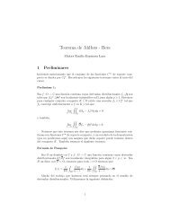
La función <strong>de</strong> <strong>de</strong>nsidad <strong><strong>de</strong>l</strong> semicírculo, ver Figura 1.1, tiene la siguiente expresión<br />
½ √<br />
4 − 2 si || ≤ 2<br />
() =<br />
0 si || 2<br />
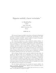
La función <strong>de</strong> distribución <strong><strong>de</strong>l</strong> semicírculo, ver Figura 1.2, está dada por<br />
⎧<br />
Z ⎨ 0 si −2<br />
1 1 1<br />
() = () = + arcsen +<br />
−∞ ⎩ 2 2 4√4 − 2 si || ≤ 2 (1.1)<br />
1 si ≥ 2<br />
5
CAPÍTULO 1. PRELIMINARES 6<br />
y<br />
2.0<br />
1.8<br />
1.6<br />
1.4<br />
1.2<br />
1.0<br />
0.8<br />
0.6<br />
0.4<br />
0.2<br />
-2.0 -1.8 -1.6 -1.4 -1.2 -1.0 -0.8 -0.6 -0.4 -0.2 0.0 0.2 0.4 0.6 0.8 1.0 1.2 1.4 1.6 1.8 2.0<br />
Figura 1.1: Función <strong>de</strong> <strong>de</strong>nsidad <strong><strong>de</strong>l</strong> semicírculo<br />
y<br />
1.0<br />
0.9<br />
0.8<br />
0.7<br />
0.6<br />
0.5<br />
0.4<br />
0.3<br />
0.2<br />
0.1<br />
-3.0 -2.8 -2.6 -2.4 -2.2 -2.0 -1.8 -1.6 -1.4 -1.2 -1.0 -0.8 -0.6 -0.4 -0.2 0.0 0.2 0.4 0.6 0.8 1.0 1.2 1.4 1.6 1.8 2.0 2.2 2.4 2.6 2.8 3.0<br />
Figura 1.2: Función <strong>de</strong> distribución <strong><strong>de</strong>l</strong> semicírculo<br />
x<br />
x
CAPÍTULO 1. PRELIMINARES 7<br />
El cálculo <strong>de</strong> los momentos <strong>de</strong> la distribución <strong><strong>de</strong>l</strong> semicírculo se <strong>de</strong>talla en el Apéndice<br />
A, en la <strong><strong>de</strong>mostración</strong> <strong><strong>de</strong>l</strong> Lema 3.<br />
Consi<strong>de</strong>remos ahora propieda<strong>de</strong>s <strong>de</strong> los eigenvalores <strong>de</strong> la matriz aleatoria.<br />
Sea la matriz aleatoria<br />
= 1<br />
√ <br />
<strong>de</strong>notemos sus eigenvalores por 12 cuya FDEE está dada por<br />
1<br />
() =<br />
# { : ≤ 1 ≤ ≤ } ∈ R (1.2)<br />
La FDEE se pue<strong>de</strong> interpretar como una función <strong>de</strong> distribución aleatoria uniforme en los<br />
eigenvalores 12 don<strong>de</strong> cada uno <strong>de</strong> estos eigenvalores tiene la probabilidad<br />
1<br />
<br />
<strong>de</strong> ocurrir.<br />
El <strong>Teorema</strong> <strong>de</strong> <strong>Wigner</strong> establece, que bajo ciertas condiciones sobre ,<br />
()<br />
<br />
−→ () ∀ ∈ R (1.3)<br />
→∞<br />
don<strong>de</strong> () está dada en 1.1.<br />
Utilizaremos el método <strong>de</strong> momentos <strong>para</strong> probar (1.3). Éste es uno <strong>de</strong> los métodos más<br />
populares en la teoría <strong>de</strong> <strong>matrices</strong> aleatorias, el cual utiliza el <strong>Teorema</strong> <strong>de</strong> convergencia <strong>de</strong><br />
momentos, i.e., consi<strong>de</strong>re una sucesión, {} ≥1 , <strong>de</strong> funciones <strong>de</strong> distribución con momentos<br />
finitos <strong>de</strong> todos los ór<strong>de</strong>nes. El <strong>Teorema</strong> <strong>de</strong> convergencia <strong>de</strong> momentos <strong>de</strong>termina bajo qué<br />
condiciones la convergencia <strong>de</strong> los momentos <strong>de</strong> todos los ór<strong>de</strong>nes implica la convergencia en<br />
distribución <strong>de</strong> la sucesión <strong>de</strong> distribuciones {} ≥1 .<br />
Denotemos el -ésimo momento <strong>de</strong> por<br />
Z<br />
= () <br />
La justificación <strong><strong>de</strong>l</strong> método <strong>de</strong> momentos lo da el siguiente lema:<br />
Lema 1 (<strong>Teorema</strong> <strong>de</strong> convergencia <strong>de</strong> momentos) <strong>Una</strong> sucesión <strong>de</strong> funciones <strong>de</strong> distribución<br />
{} converge débilmente a una función <strong>de</strong> distribución, i.e.,<br />
() −→<br />
→∞ () <br />
<strong>para</strong> todo punto <strong>de</strong> continuidad <strong>de</strong> si se satisfacen las siguientes condiciones:<br />
i) Cada tiene momentos <strong>de</strong> todos los ór<strong>de</strong>nes.<br />
ii) Para cada ≥ 0, Z<br />
Z<br />
() −→<br />
→∞<br />
() <br />
iii) está <strong>de</strong>terminada <strong>de</strong> manera única por sus momentos.
CAPÍTULO 1. PRELIMINARES 8<br />
Cuando aplicamos el Lema 1, necesitamos verificar la condición (iii) <strong><strong>de</strong>l</strong> lema anterior.<br />
El siguiente lema da una condición que implica (iii) <strong><strong>de</strong>l</strong> Lema 1.<br />
Lema 2 Sea { } ≥1 la sucesión <strong>de</strong> los momentos <strong>de</strong> la función <strong>de</strong> distribución Si<br />
1<br />
lim inf<br />
−→∞ <br />
entonces está <strong>de</strong>terminada <strong>de</strong> manera única por su sucesión <strong>de</strong> momentos {} ≥0 <br />
La <strong><strong>de</strong>mostración</strong> <strong>de</strong> los Lemas 1 y 2 se encuentran en el Apéndice B <strong>de</strong> [3].<br />
1<br />
2<br />
2 ∞ (1.4)<br />
Las condiciones sobre las variables aleatorias 11 y 12 no se relajarán más allá <strong>de</strong> pedir<br />
momento finito <strong>de</strong> or<strong>de</strong>n 4+0 1 <strong>para</strong> 11 ymomentofinito <strong>de</strong> or<strong>de</strong>n 6+ 0 1<br />
<strong>para</strong> 12 Es más simple trabajar con variables aleatorias que tengan todos los momentos<br />
finitos, con este fin utilizaremos variables aleatorias truncadas <strong>de</strong> 11 y 12 las cuales tendrán<br />
todos sus momentos.<br />
El método <strong>de</strong> truncamiento consiste en truncar la variable aleatoria <strong>de</strong> interés, en un<br />
valor <strong>de</strong>terminado, <strong>de</strong> manera que la nueva variable aleatoria tenga todos sus momentos,<br />
lo cual se cumple si <strong>de</strong>finimos ¯ como<br />
¯ =<br />
Po<strong>de</strong>mos ver que ¯ ¯<br />
¯¯ ¯ ∞ ya que<br />
¯ ¯ ¯ Z ∞<br />
= |¯| Z<br />
() =<br />
−∞<br />
||<br />
½ si || <br />
0 otro caso.<br />
|| () ≤ ¡¯ ¯ ¯ ¯ ¯ ¢ ∞ ∀ ≥ 1<br />
don<strong>de</strong> es una función <strong>de</strong> distribución. La probabilidad ¡ 6= ¯ ¢ = (|| ≥ ) siempre<br />
se pue<strong>de</strong> hacer arbitrariamente pequeña, eligiendo un valor apropiado <strong>de</strong> <br />
Antes <strong>de</strong> continuar, necesitamos discutir los momentos <strong>de</strong> la distribución <strong><strong>de</strong>l</strong> semicírculo.<br />
ElLema3dicequelosmomentospares, =2 <strong>de</strong> la distribución <strong><strong>de</strong>l</strong> semicírculo están<br />
dados por<br />
2 = = 1<br />
µ <br />
2<br />
≥ 0<br />
+1 <br />
y 2+1 =0<br />
Observemos que<br />
=<br />
1 (2)!<br />
+1!!<br />
[1 × 3 × 5 ×···×(2 − 1)] [2 × 4 × 6 ×···×2]<br />
!!<br />
[2 × 4 × 6 ×···×2]2 [1 × 2 × 3 ×···×]<br />
=2<br />
!!<br />
2 =4 <br />
Sesigueentoncesquelosnúmeros<strong>de</strong>Catalan,i.e., los momentos pares <strong>de</strong> la distribución<br />
<strong><strong>de</strong>l</strong> semicírculo, cumplen la condición 1.4, i.e.,<br />
1 1<br />
1 1<br />
1<br />
2<br />
2<br />
lim inf 2 = lim inf ≤ lim inf<br />
−→∞ −→∞ −→∞ (4 ) 1<br />
2 =0 ∞<br />
lo que nos garantiza, <strong>de</strong> acuerdo con el Lema 2 que la distribución <strong><strong>de</strong>l</strong> semicírculo está<br />
<strong>de</strong>terminada <strong>de</strong> manera única por sus momentos. Esto nos da () <strong><strong>de</strong>l</strong> Lema 1.
CAPÍTULO 1. PRELIMINARES 9<br />
1.1 Distribución <strong><strong>de</strong>l</strong> semicírculo<br />
A partir <strong>de</strong> la década <strong>de</strong> los 50’s la distribución <strong><strong>de</strong>l</strong> semicírculo, también conocida como<br />
distribución <strong>de</strong> <strong>Wigner</strong>, ha surgido <strong>de</strong> manera relevante en Teoría <strong>de</strong> probabilidad y en<br />
diversas áreas <strong>de</strong> las matemáticas. En la Teoría <strong>de</strong> Probabilidad libre ésta juega el papel que<br />
tiene la distribución normal en la Teoría <strong>de</strong> Probabilidad clásica. <strong>Una</strong> <strong>de</strong> sus aplicaciones<br />
más importantes la tiene en la Teoría <strong>de</strong> Matrices Aleatorias, don<strong>de</strong> esta distribución aparece<br />
como límite <strong>de</strong> la distribución espectral <strong>de</strong> <strong>matrices</strong> aleatorias.<br />
Lema 3 Los momentos pares <strong>de</strong> la distribución <strong><strong>de</strong>l</strong> semicírculo están dados por los números<br />
¢<br />
esto es<br />
<strong>de</strong> Catalan = 1<br />
¡ 2<br />
+1 <br />
Z 2<br />
−2<br />
2 1 √<br />
4 − 2 = <br />
2<br />
Los momentos impares son cero por la simetría <strong>de</strong> la distribución.<br />
1.2 Números <strong>de</strong> Catalan<br />
Los números <strong>de</strong> Catalan son la solución <strong>de</strong> varios problemas en diferentes áreas <strong>de</strong> las<br />
matemáticas, <strong>de</strong>ben su nombre al matemático Belga Eugéne Charles Catalan, quien los<br />
“<strong>de</strong>scubrió” en 1838 mientras estudiaba el problema <strong>de</strong> las sucesiones <strong>de</strong> paréntesis bien formados.<br />
Aunque estos números fueron nombrados en honor a Catalan, ya se conocían antes<br />
<strong>de</strong> él; alre<strong>de</strong>dor <strong>de</strong> 1751 Leonhard Euler, los <strong>de</strong>scubrió mientras estudiaba el problema <strong>de</strong> la<br />
triangulación <strong>de</strong> polígonos convexos.<br />
Los número <strong>de</strong> Catalan están <strong>de</strong>finidos como<br />
= 1<br />
µ <br />
2<br />
<br />
+1 <br />
Veamos algunos ejemplos <strong>para</strong> =3 En este caso 3 =5.<br />
Los números <strong>de</strong> Catalan cuentan el número <strong>de</strong> expresiones que contienen pares <strong>de</strong><br />
paréntesis correctamente colocados, por ejemplo <strong>para</strong> =3<br />
((())) ()(()) ()()() (())() (()())<br />
<strong>Una</strong> triangulación <strong>de</strong> un polígono esunamanera<strong>de</strong><strong>de</strong>scomponerlocomounaunión<br />
disjunta <strong>de</strong> triángulos, cuyos vértices coinci<strong>de</strong>n con los <strong><strong>de</strong>l</strong> polígono. El número <strong>de</strong> formas<br />
distintas <strong>de</strong> cortar un polígono convexo <strong>de</strong> +2 lados en triángulos conectando vértices con<br />
líneas rectas sin que ninguna se corte también está dado por los números <strong>de</strong> Catalan. La<br />
Figura 1.3 ilustra el caso <strong>de</strong> los polígonos <strong>de</strong> 5=3+2lados.<br />
Un camino <strong>de</strong> Dyck es el resultado <strong>de</strong> una caminata con 2 pasos<strong><strong>de</strong>l</strong>ongitudconstantey<br />
en las direcciones noreste y sureste, y <strong>de</strong> manera tal que nunca nos encontramos en un punto<br />
con altura menor a la altura que teníamos al inicio <strong><strong>de</strong>l</strong> recorrido y se termina el recorrido<br />
a la altura en don<strong>de</strong> se inició. Estas trayectorias también las contamos con los números <strong>de</strong><br />
Catalan. En la Figura 1.4 se observan las cinco caminatas <strong>de</strong> 6 pasos.
CAPÍTULO 1. PRELIMINARES 10<br />
Figura 1.3: Las cinco diferentes triangulaciones <strong>de</strong> un pentágono.<br />
Figura 1.4: Caminos <strong>de</strong> Dyck.
CAPÍTULO 1. PRELIMINARES 11<br />
1.3 Gráficas<br />
Figura 1.5: Gráfica conexa con un ciclo.<br />
Con el fin <strong>de</strong> calcular los límites <strong>de</strong> los momentos <strong>de</strong> la FDEE <strong>de</strong> una matriz <strong>de</strong> <strong>Wigner</strong>,<br />
necesitaremos utilizar algunas herramientas <strong>de</strong> teoría <strong>de</strong> gráficas. Esto es necesario porque<br />
la media y la varianza <strong>de</strong> cada momento empírico quedará expresado como una suma <strong>de</strong><br />
esperanzas <strong>de</strong> producto <strong>de</strong> las componentes <strong>de</strong> la matriz. A cada término <strong>de</strong> esta suma<br />
le asociamos una gráfica lo que permitirá contar sistemáticamente el número <strong>de</strong> términos<br />
significativos. Por este motivo, introduciremos algunos conceptos <strong>de</strong> teoría <strong>de</strong> gráficas y<br />
estableceremos algunos lemas. Se recomienda el libro <strong>de</strong> teoría <strong>de</strong> gráficas[4],laParte3<strong>de</strong><br />
[6], y el Capítulo 9 <strong>de</strong> [11] <strong>para</strong> una introducción a la teoría <strong>de</strong> gráficas.<br />
Definición 4 Sea un conjunto finito no vacío, ⊂ × El par () es una gráfica<br />
dirigida (digráfica) sobre , don<strong>de</strong> es el conjunto <strong>de</strong> vértices y es el conjunto <strong>de</strong> aristas.<br />
Usaremos la notación =() <br />
Si no se toma en cuenta la dirección <strong>de</strong> las aristas, será un conjunto <strong>de</strong> pares no<br />
or<strong>de</strong>nados <strong>de</strong> × ydiremosque =() es una gráfica no dirigida. En una gráfica no<br />
dirigida <strong>de</strong>notaremos las aristas por { } = { } <br />
Definición 5 Sea =() una gráfica, una arista ( ) ∈ es inci<strong>de</strong>nte a ∈ si<br />
∈ { } Para cualquier vértice ∈ se <strong>de</strong>fine grad () como el número <strong>de</strong> aristas en <br />
que son inci<strong>de</strong>ntes con <br />
Definición 6 Sean vértices <strong>de</strong> una gráfica no dirigida =() Llamaremos camino<br />
- en a una sucesión finita 12 = {+1} 1 ≤ ≤ 1 = +1 = Si<br />
en un camino - se tiene que = se dice que el camino es un ciclo (camino cerrado), en<br />
otro caso es camino abierto. Un ciclo <strong>de</strong> la forma ( ) se llamará lazo. <strong>Una</strong>gráfica cuyas<br />
aristas forman un cíclo se llamará gráfica cíclica.<br />
Definition 7 Sea =() una gráfica no dirigida. es conexa si existe un camino<br />
entre cualesquiera dos vértices <strong>de</strong> <br />
Las gráficas cíclicas son conexas.
CAPÍTULO 1. PRELIMINARES 12<br />
Figura 1.6: Gráfica conexa con un lazo.<br />
Figura 1.7: Gráfica no conexa.<br />
Figura 1.8: Gráfica y su esqueleto ˜.
CAPÍTULO 1. PRELIMINARES 13<br />
Definición 8 Sea =() una gráfica y sea ( ) ∈ al número, ≥ 1 <strong>de</strong> veces que<br />
se repite ( ) más el número <strong>de</strong> veces que se repite ( ) se le llamará multiplicidad <strong>de</strong> la<br />
arista ( ) obsérvese que la multiplicidad <strong>de</strong> ( ) es igual a la multiplicidad <strong>de</strong> la arista<br />
( ) si ésta existe Diremosqueunaaristaessimple si su multiplicidad es 1. La gráfica<br />
será una multigráfica si existe una arista en con multiplicidad mayor o igual que 2.<br />
Definición 9 El esqueleto ˜ ³ ´<br />
= ˜˜ <strong>de</strong> una gráfica dirigida =() es la gráfica<br />
obtenida <strong>de</strong> sin tomar en cuenta las direcciones <strong>de</strong> las aristas, ni las aristas repetidas.<br />
Diremos que una gráfica dirigida es conexa cuando el esqueleto es conexo.<br />
El lema siguiente nos dice que una gráfica conexa no tiene más vértices que aristas excepto<br />
en el caso <strong>de</strong> los árboles don<strong>de</strong> el número <strong>de</strong> vértices es mayor en uno que el número <strong>de</strong> aristas<br />
(ver Lema 24).<br />
Utilizaremos |·| <strong>para</strong> indicar cardinalidad <strong>de</strong> un conjunto.<br />
Lema 10 Si =() es una gráfica conexa entonces<br />
| | ≤ || +1<br />
1.3.1 De la traza a las gráficas cíclicas<br />
Consi<strong>de</strong>remos la traza <strong>de</strong> la potencia -ésima <strong>de</strong> una matriz cuadrada, ≥ 1<br />
Sea =() 1≤ ≤ una matriz.<br />
Sean<br />
i =(1 ) ∈ {1 2 } <br />
X<br />
=<br />
<br />
X<br />
1=1<br />
=<br />
X<br />
<br />
1=1<br />
X<br />
=1<br />
Lema 11 En cualquier matriz <strong>de</strong> × se cumple que<br />
¡ ¢<br />
11 =<br />
X<br />
2=1<br />
12231<br />
Del Lema 11 po<strong>de</strong>mos escribir la traza <strong>de</strong> la -ésima potencia <strong>de</strong> como<br />
tr ¡ ¢ =<br />
=<br />
X ¡ <br />
¢<br />
1=1<br />
X<br />
1=1<br />
11 =<br />
X<br />
X<br />
1=1 2=1<br />
1223 ···1<br />
12231<br />
(1.5)
CAPÍTULO 1. PRELIMINARES 14<br />
Figura 1.9: Gráfica cíclica inducida por la traza.<br />
Nótese que los subíndices <strong>de</strong> los términos <strong>de</strong> la sumatoria, i.e., (12) (23) (1)<br />
se pue<strong>de</strong>n asociar a las aristas dirigidas <strong>de</strong> una gráfica que en sí misma es un ciclo <strong>de</strong><br />
longitud . Así, la estructura cíclica que la traza induce, permite i<strong>de</strong>ntificar a cada índice<br />
i = (1 ) ∈ {1 } <strong>de</strong> la suma en la ecuación 1.5 con una gráfica conexa cíclica,<br />
(i) =( (i) (i)) don<strong>de</strong><br />
don<strong>de</strong> 1 ≤ ≤ 1 ≤ ≤ <br />
Para ≥ 1 ≥ 1 sea<br />
(i) = {12 } vértices,<br />
(i) = {(12) (23) (1)} aristas dirigidas.<br />
Λ = {() : = {12 } = {1 } =(+1) 1 ≤ ≤ 1 ≤ ≤ } <br />
(1.6)<br />
conlaconvención<strong>de</strong>que+1 = 1<br />
Para 1 ≤ ≤ Sea Λ = {() ∈ Λ : | | = } entonces se cumple que Λ1 ∩<br />
Λ2 = ∅ si 1 6= 2 por lo que<br />
siendo esta unión ajena.<br />
Λ =<br />
[<br />
=1<br />
Λ<br />
Definición 12 Dos gráficas 1 =(11) y 2 =(22) son isomorfas, <strong>de</strong>notado por<br />
1 ∼ = 2 si existe una biyección : 1 −→ 2 tal que ( ) ∈ 1 ⇐⇒ ( () ()) ∈ 2<br />
Lema 13 La relación “ ∼ =” es una relación <strong>de</strong> equivalencia en Λ
CAPÍTULO 1. PRELIMINARES 15<br />
Figura 1.10: <strong>Una</strong> gráfica <strong>de</strong> Λ85<br />
Figura 1.11: Gráfica canónica<br />
Definición 14 Llamaremos a una gráfica Γ-canónica si ésta tiene las siguientes propieda<strong>de</strong>s:<br />
1. El conjunto <strong>de</strong> vértices es = {1 } <br />
2. Existe una función <strong>de</strong> {1 } sobre {1} tal que (1) = 1 y<br />
3. Las aristas <strong>de</strong> son <strong>de</strong> la forma:<br />
() ≤ max { (1) ( − 1)} +1 <strong>para</strong> 2 ≤ ≤ <br />
=( () ( +1)) <strong>para</strong> =1 <br />
con la convención <strong>de</strong> que ( +1)= (1) = 1<br />
Sea ≤ ≤ tal que () = y ≤ la condición 3 nos garantiza que antes<br />
<strong>de</strong> llegar al vértice no se pue<strong>de</strong> llegar por primera vez a sin pasar antes por <br />
Proposición 15 Cada clase <strong>de</strong> equivalencia contiene una, y solo una, gráfica Γ-canónica<br />
La Proposición 15 es consecuencia <strong>de</strong> los siguientes dos lemas.<br />
Lema 16 Dos gráficas Γ-canónicas no son equivalentes.<br />
Sea el número <strong>de</strong> clases <strong>de</strong> equivalencia en Λ que induce “ ∼ =”.<br />
Denotemos por Γ con =1 2 las distintas ghráficas Γ-canónicas.<br />
Lema 17 Si ∈ Λ entonces ∈ [Γ] <strong>para</strong> algún 1 ≤ ≤ <br />
Ejemplo 18 Sea una ∈ Λ85 =({1 2 3 5 7} {(3 1) (1 7) (7 5) (5 5) (5 2) (2 7) (<br />
7 1) (1 3)}) esta gráfica es equivalente a gráfica Γ85-canónica ({1 5} {(1 2) (2 3) (3 4)<br />
(4 4) (4 5) (5 3) (3 2) (2 1)}) ver Figura 1.10.
CAPÍTULO 1. PRELIMINARES 16<br />
Figura 1.12: Árbol.<br />
Dado que |Λ| = ∞ yqueΛ ⊂ Λ se sigue que |Λ| ∞ por lo tanto,<br />
<strong>de</strong> acuerdo con la Proposición 15, po<strong>de</strong>mos tomar a cada gráfica canónica como elemento<br />
representante. De esta manera obtenemos la siguiente partición <strong>de</strong> Λ<br />
Λ =<br />
[<br />
=1<br />
[Γ] <br />
don<strong>de</strong> Γ, 1 ≤ ≤ es una enumeración <strong>de</strong> las gráficas Γ-canónicas.<br />
Lema 19 El número <strong>de</strong> elementos <strong>de</strong> cada clase <strong>de</strong> equivalencia <strong>de</strong> Λ es<br />
|[Γ]| = = ! ( − )!<br />
Proposición 20 El número <strong>de</strong> elementos <strong>de</strong> Λ es<br />
|Λ| = <br />
Observemos que = |Λ| = P <br />
=1 <br />
Lema 21 Sea (i) ∈ Λ con par y = <br />
2<br />
2 aristas simples.<br />
Lema 22 Sea (i) ∈ Λ con impar y = £ <br />
2<br />
tiene al menos 2 − 1 aristas simples.<br />
Definición 23 Un árbol es una gráfica conexa sin ciclos.<br />
<br />
+ , 2 ≤ ≤ entonces (i) tiene al menos<br />
2<br />
¤ £ ¤<br />
<br />
+ , 2 ≤ ≤ +1 entonces (i)<br />
2<br />
Lema 24 Si =() es una gráfica conexa no dirigida entonces | | = || +1 si, y sólo<br />
si, es árbol.
CAPÍTULO 1. PRELIMINARES 17<br />
Figura 1.13: Árboles con tres aristas orientados con raíz.<br />
Un árbol con raíz es un árbol al que se le ha especificado un vértice al que llamaremos<br />
raíz. Unárbol orientado con raíz es un árbol con raíz inmerso en un plano, cuyo contorno se<br />
recorre sobre el plano siempre en un mismo sentido previamente convenido, <strong>de</strong> la siguiente<br />
manera: el recorrido inicia y termina en la raíz, al término <strong><strong>de</strong>l</strong> recorrido se recorre la misma<br />
cantidad <strong>de</strong> aristas <strong>de</strong> ida que <strong>de</strong> vuelta y en cada paso <strong><strong>de</strong>l</strong> recorrido no se tienen más aristas<br />
recorridas <strong>de</strong> vuelta que <strong>de</strong> ida. El propósito es contar el número <strong>de</strong> árboles orientados con<br />
raíz.<br />
A cada árbol orientado con raíz <strong>de</strong> aristas lo i<strong>de</strong>ntificamos con la 2-tupla ( 1 2)<br />
construida <strong>de</strong> la siguiente manera, si en el -ésimo paso <strong><strong>de</strong>l</strong> recorrido la arista en turno es<br />
recorrida por primera vez entonces =1y si ya se había pasado por ella entonces = −1.<br />
Estonosdaunabiyecciónentrelosárbolesorientadosconraíz<strong>de</strong> aristas y el subconjunto<br />
2 <strong>de</strong> {−1 1} 2 que consta <strong>de</strong> los elementos ( 1 2) tales que<br />
= ±1<br />
1 + 2 + + 2 = 0<br />
1 + 2 + + ≥ 0 =1 2 2 (1.7)<br />
Lasegundacondicióngarantizaqueelrecorridoiniciayterminaenlaraíz,yqueal<br />
término <strong><strong>de</strong>l</strong> recorrido el número <strong>de</strong> aristas que se recorren <strong>de</strong> ida sea igual a los que se<br />
recorren <strong>de</strong> vuelta, la tercera condición indica que en cualquier parte <strong><strong>de</strong>l</strong> recorrido nunca se<br />
recorren más aristas <strong>de</strong> regreso.<br />
En la Figura 1.13 se muestran los cinco árboles orientados con raíz con tres aristas, a los<br />
cuales les correspon<strong>de</strong>n (1 1 1 −1 −1 −1) (1 1 −1 −1 1 −1) (1 −1 1 1 −1 −1) (1 1<br />
−1 1 −1 −1) (1 −1 1 −1 1 −1) respectivamente.<br />
La sucesión <strong>de</strong> 1 2 nos servirá <strong>para</strong> encontrar una biyección entre los árboles dirigidos<br />
con raíz y los árboles binarios, los cuales los contaremos <strong>de</strong> manera similar.<br />
Un árbol binario es un árbol en el que todo vértice tiene grado uno, dos o tres. A un<br />
vértice con grado dos se le llama padre inicial, aunvérticecongradotresselellamapadre;<br />
yselellamahijo a un vértice con grado uno. Cada padre tiene dos hijos llamados hijo <strong>de</strong><br />
la <strong>de</strong>recha e hijo <strong>de</strong> la izquierda.<br />
De manera similar que en el caso <strong>de</strong> los árboles con raíz, po<strong>de</strong>mos contar los árboles<br />
binarios con padres, i<strong>de</strong>ntificándolos también con 2-tuplas. Para esto, recorreremos el<br />
árbol binario iniciando por la arista que une al padre inicial (vértice con dos árboles) con<br />
su hijo <strong>de</strong> la <strong>de</strong>recha. A cada árbol binario le asociamos la 2-tupla ( 0<br />
1 0<br />
2), lacual<br />
construimos <strong>de</strong> la siguiente manera: partiendo <strong><strong>de</strong>l</strong> padre inicial recorremos en sentido horario,<br />
si la arista por la que pasamos conecta al hijo <strong>de</strong> la <strong>de</strong>recha hacemos 0<br />
=1y si conecta con<br />
el hijo <strong>de</strong> la izquierda 0<br />
= −1 no se contabilizan los hijos por los que ya se hayan pasado.
CAPÍTULO 1. PRELIMINARES 18<br />
Figura 1.14: Árboles binarios con 3 padres.<br />
Consi<strong>de</strong>rando los cinco árboles binarios con tres padres a los que les asociamos (1 −1<br />
1 −1 1 −1) (1 −1 1 1 −1 −1) (1 1 −1 −1 1 −1) (1 1 1 −1 −1 −1) (1 1 −1 1 −1<br />
−1)<br />
Claramente esta sucesión 0<br />
1 0<br />
2 es una permutación válida <strong>de</strong> la sucesión 1 2, y<br />
cumple (1.7), por lo que se tiene una biyección entre 0<br />
1 0<br />
2 y 1 2 Esto nos da una<br />
biyección entre los árboles orientados con raíz y los árboles binarios.<br />
Proposición 25 Hay árboles binarios con padres.<br />
Proposición 26 El número <strong>de</strong> árboles orientados con raíz que se pue<strong>de</strong>n formar con <br />
aristas es igual al −ésimonúmero<strong>de</strong>Catalan.<br />
1.3.2 Procedimiento <strong>de</strong> truncamiento<br />
Este procedimiento consiste en truncar variables aleatorias <strong>para</strong> trabajar con variables aleatorias<br />
que tengan momentos finitos.<br />
Sea el -ésimo momento <strong>de</strong> or<strong>de</strong>n <strong>de</strong> dada en (1.2) entonces<br />
Z<br />
: = <br />
X 1<br />
() = <br />
<br />
<br />
= tr( )<br />
=<br />
µ ³ ´ <br />
<br />
1 tr √ <br />
<br />
=<br />
1<br />
<br />
1+ 2<br />
X<br />
12=1<br />
=1<br />
1223 1<br />
Vamos a truncar las variables en √ <strong>para</strong> obtener las nuevas variables ¯, con<br />
½<br />
si || <br />
¯ =<br />
√ <br />
0 si || ≥ √ <br />
y<strong>de</strong>finamos<br />
Z<br />
¯ := ¯ X X<br />
1<br />
() = ¯12 ¯23 ¯1 (1.8)<br />
1+ 2<br />
1=1<br />
=1
CAPÍTULO 1. PRELIMINARES 19<br />
Tenemos que la esperanza <strong>de</strong> ¯ se pue<strong>de</strong> escribir como<br />
¡ ¢ 1<br />
¯ = <br />
1+ 2<br />
X<br />
1=1<br />
(¯12 ¯23 ¯1) = 1<br />
<br />
1+ 2<br />
don<strong>de</strong> ( (i)) = (¯12 ¯23 ¯1) <br />
En el <strong>de</strong>sarrollo <strong>de</strong> la <strong><strong>de</strong>mostración</strong> usaremos los siguientes Lemas.<br />
X<br />
( (i)) (1.9)<br />
Lema 27 Sea una función <strong>de</strong> distribución, si R ∞<br />
−∞ || () ∞, y ≥ 1 entonces, se<br />
tienen los siguientes resultados<br />
()<br />
()<br />
()<br />
lim<br />
→∞ (−)2<br />
Z<br />
|| √ <br />
<br />
() ∞ ∀ ≥ +1<br />
Z<br />
lim<br />
→∞<br />
||≥ √ ||<br />
<br />
() =0<br />
µ<br />
lim<br />
→∞<br />
(−1)2<br />
Z<br />
||≥ √ <br />
()<br />
<br />
=0<br />
Lema 28 Sea una función <strong>de</strong> distribución, si R ∞<br />
−∞ || () ∞ ≥ 1 y R () =<br />
0 entonces, se cumple el siguiente límite<br />
µ<br />
lim<br />
→∞<br />
(−1)2<br />
Z<br />
|| √ <br />
<br />
() =0<br />
Lema 29 Sea una función <strong>de</strong> distribución. Si R ∞<br />
−∞ ||+ () ∞ 0 0 y<br />
0 tal que + entonces el siguiente límite es cierto<br />
Z<br />
() =0<br />
−<br />
lim 2<br />
−→∞<br />
|| √ <br />
1.3.3 Operaciones con aristas <strong>de</strong> una gráfica<br />
Consi<strong>de</strong>remos una gráfica (i) ∈ Λ Denotemos por el número <strong>de</strong> aristas con multiplicidad<br />
en (i) 1 ≤ ≤ − +1ypor el número <strong>de</strong> lazos <strong>de</strong> multiplicidad <br />
1 ≤ ≤ − y cumplen que<br />
−+1 X<br />
=1<br />
( + ) = ≥ − 1 ≥ 0<br />
()
CAPÍTULO 1. PRELIMINARES 20<br />
Los valores <strong>de</strong> ( (i)) se <strong>de</strong>terminan sólo con los valores <strong>de</strong> y <strong>de</strong> la siguiente manera<br />
( (i)) =<br />
−+1 Y<br />
=1<br />
¡ ¢ <br />
¯ 12<br />
¡ ¯ <br />
¢<br />
11 (1.10)<br />
Tomando en cuenta que ¯ <br />
12 ∞ <strong>para</strong> 1 ≤ ≤ ¯12 −→ 0 y ¯<br />
→∞ <br />
11 ∞ <strong>para</strong> 1 ≤ ≤ ,<br />
motivadosporloslemas27() y 28 escribiremos la siguiente <strong>de</strong>scomposición <strong>de</strong> ( (i))<br />
( (i)) =<br />
don<strong>de</strong><br />
y<br />
³ −1<br />
−<br />
2 −1 ´ 1<br />
2 ¯12<br />
×<br />
−+1 Y<br />
=+1<br />
= 1− 1<br />
1+<br />
2 2<br />
×<br />
( (i)) =<br />
Supongamos que<br />
−+1 Y<br />
=+1<br />
à Y<br />
=2<br />
³ −<br />
−<br />
2 −<br />
2 ¯ <br />
12<br />
¡ ¢ <br />
¯ 12<br />
´ − Y<br />
=+1<br />
−+1 1 − =+1 (−)+ 2 =+1 (−)<br />
!Ã Y<br />
=1<br />
³<br />
−<br />
2 ¯ <br />
´ <br />
12<br />
− Y ³<br />
<br />
=+1<br />
−<br />
2 ¯ <br />
´ <br />
11<br />
¡ ¢ <br />
¯ 11<br />
!<br />
×<br />
³ −<br />
−<br />
2 −<br />
2 ¯ <br />
´ <br />
11<br />
³<br />
−1 ´ 1<br />
2 ¯12 ×<br />
Y<br />
=2<br />
¡ ¢ <br />
¯ 12<br />
Y<br />
=1<br />
¡ ¢ <br />
¯ 11<br />
= (()) ( (i)) (1.11)<br />
X<br />
( (i)) = 1<br />
2 (1 − ) 1 + 1<br />
−+1<br />
2<br />
³<br />
−1 ´ ()1<br />
2 ¯12<br />
×<br />
Y<br />
=2<br />
¡ ¢ ()<br />
¯ 12<br />
=+1<br />
−+1 Y<br />
=+1<br />
Y<br />
=1<br />
( − ) + 1<br />
2<br />
³<br />
−<br />
2 ¯ <br />
´ ()<br />
12<br />
¡ ¢ ()<br />
¯ 11 <br />
: = lim<br />
→∞ sup {| (i)|} ∞<br />
()<br />
− X<br />
=+1<br />
− Y<br />
=+1<br />
( − ) <br />
³<br />
−<br />
2 ¯ <br />
´ ()<br />
11<br />
(1.12)<br />
Entonces<br />
( (i)) ≤ (()) (1.13)<br />
Así<br />
¡ ¢<br />
¯<br />
1 X<br />
= ( (i)) ≤<br />
1+ 2<br />
()<br />
<br />
X<br />
<br />
1+ 2<br />
()<br />
(()) <br />
Observemos que si encontramos cotas <strong>para</strong> los valores <strong>de</strong> ( (i)) esto nos pue<strong>de</strong> ayudar<br />
asimplificar la expresión X<br />
[()] <br />
()
CAPÍTULO 1. PRELIMINARES 21<br />
lo que será <strong>de</strong> utilidad en la <strong><strong>de</strong>mostración</strong> <strong><strong>de</strong>l</strong> <strong>Teorema</strong> <strong>de</strong> <strong>Wigner</strong>.<br />
La función [ (i)] dada en (1.12) se pue<strong>de</strong> calcular <strong>para</strong> cualquier gráfica con aristas.<br />
Sea Υ () =( ()) 6= ∅ | | ∞ una gráfica con aristas.<br />
Sea () ={12}<br />
Si ∈ () <strong>de</strong>finimos la resta <strong>de</strong>unaaristaalagráfica Υ () como Υ ()− =({12<br />
−1+1 })<br />
Si =( ) <strong>de</strong>finimos la suma <strong>de</strong>unaaristaalagráfica Υ () comoΥ ()+ =( ∪{ } <br />
{12 ( )}) Si ∈ () diremos que se crea una arista.<br />
La <strong>de</strong>finición <strong>de</strong> [ (i)] dada en (1.12) se pue<strong>de</strong> exten<strong>de</strong>r a gráficas arbitrarias con aristas.<br />
Sean ≥ 0 y ≥ 0 el número <strong>de</strong> aristas y lazos <strong>de</strong> la gráfica (i), respectivamente, con<br />
multiplicidad .<br />
Se cumple que P<br />
( + ) =<br />
=1<br />
Sea ≥ 2 ≥ 1 Definamos la función<br />
[Υ ()] = 1<br />
2 (1 − ) 1 + 1<br />
2<br />
X<br />
=+1<br />
( − ) + 1<br />
2<br />
X<br />
=+1<br />
( − ) <br />
Estudiaremos el efecto en [Υ ()] <strong>de</strong> la resta y la suma <strong>de</strong> aristas a la gráfica Υ () <br />
Observemosquelosvalores<strong>de</strong>2 y<strong>de</strong>1 no se utilizan en [Υ ()] Entonces<br />
al restar o sumar aristas a una gráfica Υ () hay que tener presente esta información.<br />
Al restar una arista <strong>de</strong> Υ () digamos una <strong>de</strong> las <strong>de</strong> multiplicidad <strong>para</strong> algún 1 ≤<br />
≤ observemos que se reduce en una unidad y que −1 se incrementa en una unidad,<br />
i.e.,<br />
−→ − 1<br />
−1 −→ −1 +1<br />
al restar un lazo <strong>de</strong> Υ () el resultado es similar.<br />
−→ − 1<br />
−1 −→ −1 +1<br />
Más a<strong><strong>de</strong>l</strong>ante se hará un procedimiento doble que consistirá primero en restar arista y<br />
<strong>de</strong>spués agregar arista, lo que se pue<strong>de</strong> interpretar como un reacomodo <strong>de</strong> arista en una<br />
gráfica.<br />
Sea ∈ () y<strong>de</strong>notemospormealamultiplicidad <strong>de</strong> Entonces<br />
⎧<br />
⎪⎨<br />
[Υ ()] −<br />
[Υ () − ] =<br />
⎪⎩<br />
1<br />
2 (1 − ) me =1<br />
[Υ ()] + 1<br />
2 (1 − ) me =2<br />
[Υ ()] 3 ≤ me ≤ <br />
me ≥ +1<br />
[Υ ()] − 1<br />
2<br />
Sea ( ) 6= unaaristaquesumaremosaΥ () esta pue<strong>de</strong> colocarse sobre una<br />
arista, con multiplicidad 1 2 Si ( ) ∈ () se crea una arista y convendremos en<br />
<strong>de</strong>cir que se colocará sobre una arista, con multiplicidad cero.
CAPÍTULO 1. PRELIMINARES 22<br />
Entonces<br />
1 2 3 ≥ +1<br />
0 0 1 − 1<br />
1 − 1 0<br />
2 − 1<br />
<br />
≥ +1<br />
<br />
2<br />
<br />
2<br />
<br />
2<br />
− 1<br />
2<br />
1 <br />
− 2<br />
1 − <br />
2<br />
1 − <br />
2<br />
2<br />
<br />
2<br />
− <br />
2<br />
− 1<br />
2<br />
<br />
−<br />
<br />
2<br />
2<br />
0 − 2 1<br />
2<br />
1<br />
2<br />
1 −<br />
2<br />
0<br />
0<br />
− 1<br />
Tabla 1.1: Valores <strong>de</strong> [Υ () − +( )] − (Υ ()) 6= <br />
1 2 3 ≥ +1<br />
0,..., − 1<br />
≥ <br />
<br />
2<br />
<br />
2<br />
− 1<br />
2<br />
1 <br />
− 2<br />
1 − <br />
2<br />
0 − 2 1<br />
2<br />
Tabla 1.2: Valores <strong>de</strong> [Υ () − +( )] − (Υ ()) <br />
⎧<br />
⎪⎨<br />
[Υ ()] +<br />
[Υ ()+( )] =<br />
⎪⎩<br />
1<br />
2 (1 − ) me =0<br />
[Υ ()] − 1<br />
2 (1 − ) me =1<br />
[Υ ()] 2 ≤ me ≤ − 1<br />
me ≥ <br />
[Υ ()] + 1<br />
2<br />
Silaaristaquesesumaráesunlazo<strong><strong>de</strong>l</strong>aforma( ) y lo colocamos en uno <strong>de</strong> multiplicidad<br />
me, i.e.,<br />
½<br />
[Υ ()] 0 ≤ me ≤ − 1<br />
[Υ ()+( )] =<br />
me ≥ <br />
1<br />
2<br />
[Υ ()] + 1<br />
2<br />
Si hacemos la operación <strong>de</strong> restar arista y <strong>de</strong>spués sumar arista obtenemos un reacomodo<br />
<strong>de</strong> arista en la gráfica Υ () Si el reacomodo es <strong>de</strong> una arista a otra arista, los valores <strong>de</strong><br />
[Υ () − +( )] 6= se pue<strong>de</strong>n ver en la Tabla 1.1<br />
Si el reacomodo es <strong>de</strong> una arista a un lazo, los valores <strong>de</strong> [Υ () − +( )] se muestran<br />
en la Tabla 1.2. Si el reacomodo es <strong>de</strong> un lazo a otro lazo, los valores <strong>de</strong> [Υ () − ( )+( )]<br />
están en la Tabla 1.3.<br />
Si el reacomodo es <strong>de</strong> un lazo a una arista, los valores [Υ () − ( )+] estánenla<br />
Tabla 1.4.<br />
1.3.4 Cotas superiores <strong>para</strong> <br />
Introduciremos el concepto <strong>de</strong> peores gráficas con el fin <strong>de</strong>simplificar la obtención <strong>de</strong> cotas<br />
<strong>para</strong> los valores <strong>de</strong> ( (i)) <br />
Para ≥ 1 y 1 ≤ ≤ consi<strong>de</strong>remos gráficas (i) ∈ Λ<br />
0
CAPÍTULO 1. PRELIMINARES 23<br />
1 a +1 ≥ +1<br />
0<br />
1 <br />
− 2 2<br />
1 − 2<br />
1 ≤ ≤ − 1 0 − 1<br />
1<br />
2<br />
<br />
≥ +1<br />
2 0 0<br />
1 0 0<br />
2<br />
− <br />
2<br />
− 1<br />
2<br />
Tabla 1.3: Valores <strong>de</strong> [Υ () − ( )+( )] − (Υ ()) <br />
1 a +1 +1<br />
0<br />
1 <br />
− 2 2<br />
1 − 1<br />
2<br />
+ <br />
2<br />
− <br />
2<br />
1+ <br />
2<br />
2 ≤ ≤ − 1 0 −1<br />
2<br />
≥ <br />
1<br />
2 0 0<br />
− <br />
2<br />
<br />
−1+<br />
− 1<br />
2<br />
Tabla 1.4: Valores <strong>de</strong> [Υ () − ( )+] − (Υ ()) <br />
Llamaremos peor gráfica aunagráfica ˆ tal que <br />
2<br />
³ ´<br />
ˆ ≥ ( (i)) ∀ (i) ∈ Λ<br />
Si =1 Λ1 tiene elementos, las gráficas <strong>de</strong> Λ1 son <strong>de</strong> la forma =({i} ) <br />
i =(1 1) con ( (i)) = ¯ 11 aquí () = 1<br />
2<br />
( − ) <br />
Para par y 2 ≤ ≤ <br />
2 la peor gráfica <strong>para</strong> estos valores <strong>de</strong> y es ˆ una gráfica<br />
con una arista <strong>de</strong> multiplicidad − 2 +4y − 2 aristas <strong>de</strong> multiplicidad 2.<br />
Lema 30 Si (i) ∈ Λ con 2 ≤ ≤ <br />
entonces<br />
2<br />
( (i)) ≤ ˆ := <br />
<br />
− +2− (1.14)<br />
2 2<br />
Para impar y 2 ≤ ≤ £ ¤<br />
+1 la peor gráfica <strong>para</strong> estos valores <strong>de</strong> y es ˆ una<br />
2<br />
gráfica con una arista <strong>de</strong> multiplicidad − 2 +4y − 2 aristas <strong>de</strong> multiplicidad 2.<br />
Lema 31 Si (i) ∈ Λ con impar y 2 ≤ ≤ £ ¤<br />
+1 entonces<br />
2<br />
( (i)) ≤ ˆ := <br />
2<br />
<br />
− +2− (1.15)<br />
2<br />
Figura 1.15: Peor gráfica ˆ con =4y =10
CAPÍTULO 1. PRELIMINARES 24<br />
Para = <br />
2<br />
Figura 1.16: Gráfica ˆ con =6y =8<br />
Figura 1.17: Gráfica ˆ 4con =6y =10<br />
+ 2 ≤ ≤ <br />
2 y par la peor gráfica <strong>para</strong> estos valores <strong>de</strong> y es ˆ<br />
la gráfica con 2 aristas simples y − 2 = <br />
2<br />
− aristas dobles.<br />
Lema 32 Si (i) ∈ Λ, conpar y = + ≥ 2 se cumple que<br />
2<br />
( (i)) ≤ ˆ := (1 − ) (1.16)<br />
Lema 33 Si (i) ∈ Λ con impar y = £ ¤<br />
+ ≥ 2 se cumple que<br />
2<br />
Sea =1+ <br />
2 y<br />
simples, una arista triple y <br />
2<br />
( (i)) ≤ ˆ := 1<br />
(1 − )(2− 1) (1.17)<br />
2<br />
¯ ˜<br />
¯ <br />
2 la peor gráfica <strong>para</strong> estos valores es ˆ la gráfica con 3 aristas<br />
− 3 aristas dobles.<br />
Lema 34 Si (i) ∈ Λ, conpar y =1+ <br />
|| 2 2<br />
( (i)) ≤ ˆ :=<br />
se cumple que<br />
3(1− )<br />
(1.18)<br />
2
Capítulo 2<br />
El <strong>Teorema</strong> <strong>de</strong> <strong>Wigner</strong><br />
Sea unamatriz<strong>de</strong><strong>Wigner</strong>real × con componentes <strong>de</strong>finidas en un espacio <strong>de</strong><br />
probabilidad (Ω F) don<strong>de</strong> Ω es el espacio muestral y es la medida <strong>de</strong> probabilidad<br />
<strong>de</strong>finida sobre la -álgebra <strong>de</strong> eventos F<br />
Los supuestos sobre las componentes <strong>de</strong> la matriz aleatoria son los siguientes:<br />
Sean y funciones <strong>de</strong> distribución reales.<br />
1. 11 ∼ y |11| 4+ ∞ 0 1<br />
2. 12 ∼ 12 =0, 2 12 =1y |12| 6+ ∞ 0 1<br />
3. = si 1 ≤ ≤ <br />
4. <br />
5. <br />
<br />
= 12 si 1 ≤ ≤ <br />
<br />
= 11 si 1 ≤ ≤ <br />
6. son v.a.i.i.d. si 1 ≤ ≤ ≤ <br />
Consi<strong>de</strong>remos la matriz<br />
= 1<br />
√ <br />
<strong>Teorema</strong> 35 (<strong>Teorema</strong> <strong>de</strong> <strong>Wigner</strong>) Sean y funciones <strong>de</strong> distribución. Si 11 ∼<br />
2 11 ∞ 12 =0 2 12 =1y 4 12 ∞, entonces la FDEE, dada en (1.2),<br />
cumple que<br />
()<br />
<br />
−→ ()<br />
→∞<br />
Si a<strong>de</strong>más , |11| 4+ ∞ 0 1 y |12| 6+ ∞ 0 1 entonces<br />
()<br />
<br />
−→ ()<br />
→∞<br />
don<strong>de</strong> () es la función <strong>de</strong> distribución <strong><strong>de</strong>l</strong> semicírculo dada en (1.1).<br />
25
CAPÍTULO 2. EL TEOREMA DE WIGNER 26<br />
2.1 Demostración <strong><strong>de</strong>l</strong> <strong>Teorema</strong> <strong>de</strong> <strong>Wigner</strong><br />
Primero aplicaremos el Lema 1 a la FDEE ¯ <strong><strong>de</strong>l</strong>as<strong>matrices</strong>aleatoriastruncadas. Para<br />
esto probaremos que ¯ dado en (1.9), cumple<br />
lim<br />
→∞ ( ¯ ½<br />
si es par,<br />
) = 2<br />
(2.1)<br />
0 si es impar,<br />
yque<br />
∞X<br />
Var ¡ ¢<br />
¯ ∞ (2.2)<br />
=1<br />
con (2.1) y (2.2) se condición (ii) <strong><strong>de</strong>l</strong> Lema 1 casi seguramente y <strong>de</strong>bido a que se cumplen<br />
(i) y (iii), con () = () <strong>de</strong> Lema 1 concluimos que<br />
¯ ()<br />
<br />
−→ () ∀ ∈ R<br />
→∞<br />
Por último, <strong>para</strong> el caso <strong>de</strong> las <strong>matrices</strong> aleatorias originales, en la Sección (2.1.3) se<br />
<strong>de</strong>muestra que P ∞<br />
=1 £¯ ¯ − ( ¯ ) ¯ ¯ ¤ ∞ lo que prueba que<br />
es <strong>de</strong>cir,<br />
lim<br />
→∞ = lim<br />
→∞<br />
<br />
<br />
−→<br />
→∞<br />
¯ <br />
½<br />
si es par,<br />
2<br />
0 si es impar.<br />
En consecuencia tenemos la condición (ii) <strong><strong>de</strong>l</strong> Lema 1 casi seguramente, por lo tanto se<br />
obtiene que<br />
<br />
() −→ () ∀ ∈ R<br />
→∞<br />
lo cual es el objetivo <strong>de</strong> esta tesis.<br />
2.1.1 Convergencia en esperanza <strong>de</strong> ¯ <br />
Descomponemos ( ¯) dada en la ecuación (1.9) <strong>de</strong> la siguiente manera<br />
don<strong>de</strong><br />
( ¯) =<br />
= 1<br />
<br />
1+ 2<br />
y ( (i)) está dada por (1.10) y (1.11).<br />
X<br />
=1<br />
X<br />
<br />
()<br />
| ˜ (())|=<br />
( (i))
CAPÍTULO 2. EL TEOREMA DE WIGNER 27<br />
Observemos lo siguiente<br />
<strong>de</strong> (1.13) obtenemos que<br />
|| ≤ 1<br />
<br />
1+ 2<br />
|| ≤<br />
1<br />
<br />
1+ 2<br />
X<br />
()<br />
| ˜ (())|=<br />
= ˆ <br />
= ˆ<br />
<br />
X<br />
()<br />
| ˜ (())|=<br />
1+ <br />
2<br />
| ( (i))|<br />
X<br />
()<br />
| ˜ (())|=<br />
<br />
ˆ <br />
<br />
1+ 2<br />
don<strong>de</strong> ˆ representa la cota superior <strong>de</strong> las ( (i)) con (i) ∈ Λ. Los términos que<br />
no <strong>de</strong>pen<strong>de</strong>n <strong>de</strong> <strong>de</strong> esta relación son y A continuación analizaremos el límite<br />
lim<br />
→∞ || ≤ lim<br />
→∞<br />
en virtud <strong>de</strong> que <strong>de</strong> que el lim→∞ <br />
=1tenemos que<br />
lim<br />
→∞ || ≤ lim<br />
→∞<br />
ˆ <br />
<br />
1+ 2<br />
1<br />
ˆ <br />
<br />
1+ 2<br />
= lim<br />
→∞ +ˆ <br />
−1− 2 (2.3)<br />
Calcularemos los límites <strong>de</strong> cuando tien<strong>de</strong> a infinito tomando en cuenta la<br />
paridad <strong>de</strong> y distintos casos <strong>para</strong> <br />
Caso 1: impar.<br />
Subcaso 1.1 =1<br />
Si =1y ≤ <br />
lim<br />
→∞ || ≤ 1<br />
<br />
1+ <br />
2<br />
X<br />
|11| =<br />
1=1<br />
|11| <br />
<br />
2<br />
−→ 0<br />
Si =1y ,entoncessólosetieneunagráfica Γ1-canónica en Λ1 y = 1 −<br />
<strong>de</strong> 2<br />
aquí que<br />
lim<br />
→∞ |1| ≤ 1 lim<br />
→∞<br />
ya que 1 = ¯ 11 ∞<br />
− <br />
1<br />
1+ −1− −<br />
2 2 = 1 lim 2<br />
→∞ =0 0
CAPÍTULO 2. EL TEOREMA DE WIGNER 28<br />
Subcaso 1.2 2 ≤ ≤ £ ¤<br />
+1 2<br />
Tenemos por el Lema 31 que cualquier gráfica (i) ∈ Λ con estos valores <strong>de</strong> y <br />
<br />
− +2− por lo que<br />
2<br />
ˆ =ˆ = <br />
2<br />
1<br />
2<br />
lim<br />
→∞ || ≤ lim<br />
→∞<br />
+ <br />
2<br />
<br />
1<br />
−+2− −1− 1− 2 2 = lim 2<br />
→∞ =02<br />
Subcaso 1.3 £ ¤<br />
+2≤ ≤ <br />
2<br />
Para = £ ¤ £ ¤<br />
<br />
<br />
+ con 2 ≤ ≤ +1 tenemos por el Lema 33 que ˆ =ˆ 2<br />
2<br />
=<br />
(1 − )(2− 1) <strong>para</strong> toda gráfica (i) con estos valores <strong>de</strong> y por lo que<br />
lim<br />
→∞ || ≤ lim<br />
→∞ [ 2]++ 1<br />
<br />
(1−)(2−1)−1− 2 2 = lim<br />
1<br />
= lim 2<br />
→∞ (−4)+(2−)<br />
= 0≥ 2≥ 4<br />
Caso 2: par<br />
Subcaso 2.1 =1 Similar al subcaso 1.1.<br />
Subcaso 2.2 2 ≤ ≤ <br />
2<br />
ElLema30nosdicequeˆ =ˆ = <br />
<br />
− +2− 2 2<br />
lim<br />
→∞ || ≤ lim<br />
→∞<br />
Subcaso 2.3 <br />
2<br />
+ <br />
2<br />
por lo que<br />
→∞<br />
1<br />
2 +2−−2<br />
<br />
1<br />
−+2− −1− 1− 2 2 = lim 2<br />
→∞ =02<br />
+2≤ ≤ <br />
Para = <br />
<br />
+ con 2 ≤ ≤ 2 2tenemos por el Lema 32 que ˆ =ˆ =(1−) <strong>de</strong><br />
don<strong>de</strong> tenemos que<br />
lim<br />
→∞ || ≤ lim<br />
→∞ +ˆ <br />
−1− 2 = lim<br />
→∞<br />
Subcaso 2.4<br />
=1+ <br />
2 <br />
En este último caso<br />
<br />
1+ =<br />
2<br />
= lim<br />
→∞ (2−)−1 =0≥ 2<br />
=<br />
1<br />
<br />
1+ 2<br />
1<br />
<br />
1+ 2<br />
X<br />
()<br />
| ˜ (())|=1+ <br />
2<br />
X<br />
()<br />
| ˜ (())|=1+ <br />
| ˜(())|= <br />
2<br />
2<br />
= ˘ 1+ <br />
2 + ˇ 1+ <br />
2 <br />
( (i))<br />
( (i)) + 1<br />
<br />
1+ 2<br />
X<br />
()<br />
| ˜ (())|=1+ <br />
| ˜(())| <br />
2<br />
2<br />
<br />
<br />
++(1−)−1−<br />
2 2<br />
( (i))
CAPÍTULO 2. EL TEOREMA DE WIGNER 29<br />
En la primera sumatoria se cuentan las gráficas con aristas cuyo esqueleto tiene <br />
2 aristas,<br />
<strong>de</strong> esto tenemos que<br />
estos son los árboles los cuales sabemos están dados por <br />
2<br />
˘ <br />
1+ =<br />
2<br />
=<br />
1<br />
<br />
1+ 2<br />
1<br />
<br />
1+ 2<br />
X<br />
()<br />
| ˜ (())|=1+ <br />
2<br />
| ˜ (())|= <br />
2<br />
X<br />
()<br />
| ˜ (())|=1+ <br />
| ˜(())|= <br />
2<br />
2<br />
( (i))<br />
<strong><strong>de</strong>l</strong> hecho <strong>de</strong> que(¯ 2 12) <br />
2 <br />
=1y<strong>de</strong>queellim <br />
→∞<br />
¯<br />
Ahora si ¯ ˜<br />
¯<br />
( (i)) ¯ <br />
Así<br />
¯ ˇ 1+ <br />
2 <br />
¯ =<br />
≤<br />
lim<br />
→∞<br />
˘ 1+ <br />
2<br />
¡ ¢ <br />
2 1<br />
2 ¯ 12 = <br />
1+ 2<br />
1+ <br />
2<br />
= <br />
2<br />
<br />
2<br />
<br />
1+ <br />
¡ ¢ <br />
2 2 ¯ 12<br />
2<br />
<br />
1+ 2 =1 se sigue que<br />
2 porelLema34setienequeˆ =ˆ = 3(1−)<br />
2<br />
1<br />
<br />
1+ 2<br />
1<br />
<br />
1+ 2<br />
X<br />
()<br />
| ˜ (())|=1+ <br />
2<br />
| ˜ (())|= <br />
2<br />
1+ <br />
2<br />
| ( (i))| ≤ 1<br />
<br />
1+ 2<br />
<br />
1+ <br />
2<br />
3(1−) <br />
1+ 2 2<br />
= <br />
1+ <br />
1+ <br />
2 2<br />
3(1−)<br />
2 −→ 01<br />
→∞<br />
lim<br />
→∞<br />
¯<br />
¯ ˇ 1+ <br />
2 <br />
¯ =01<br />
1+ <br />
2<br />
En consecuencia<br />
lim<br />
→∞ 1+ <br />
= 2<br />
2<br />
En resumen hemos probado que <strong>para</strong> ∈ N, 1 ≤ ≤ se cumple<br />
lim<br />
→∞ <br />
½<br />
si =1+<br />
= 2<br />
<br />
par,<br />
2<br />
0 otro caso.<br />
Por lo tanto la esperanza <strong>de</strong> ¡ ¢ P<br />
¯<br />
<br />
= =1 se simplifica en<br />
lim<br />
→∞ ¡ ½<br />
¢ si par,<br />
¯ = 2<br />
0 otro caso.<br />
<br />
1+ <br />
2<br />
<br />
1+ <br />
2<br />
ˆ <br />
(2.4)
CAPÍTULO 2. EL TEOREMA DE WIGNER 30<br />
2.1.2 Convergencia casi segura <strong>de</strong> ¯ <br />
En esta sección probaremos que<br />
Para esto observemos que<br />
Var ¡ ¢<br />
<br />
¯ =<br />
=<br />
=<br />
∞X<br />
=1<br />
Var ¡ ¢<br />
<br />
¯ ∞<br />
⎛<br />
1<br />
Var ⎝<br />
+2 X<br />
⎞<br />
¯12¯1<br />
⎠<br />
()<br />
⎛<br />
1<br />
⎝<br />
+2 X<br />
⎡<br />
¯12¯1 − ⎣<br />
()<br />
X<br />
⎤⎞<br />
(¯12¯1) ⎦⎠<br />
()<br />
⎛<br />
1<br />
⎝<br />
+2 X<br />
¯12¯1 − X<br />
⎞2<br />
( (i)) ⎠<br />
()<br />
<strong>de</strong>sarrollando el binomio al cuadrado, llegamos a que<br />
Var ¡ ⎡<br />
¢<br />
¯<br />
1<br />
= ⎣<br />
+2 X X<br />
¯12¯1¯12¯1<br />
() ()<br />
−2 X X<br />
¯12¯1 ()+ X<br />
⎤<br />
X<br />
( (i)) ( (j)) ⎦ <br />
()<br />
()<br />
()<br />
() ()<br />
dado que P P<br />
¯12¯1 () =<br />
()<br />
()<br />
P P<br />
( (i)) ( (j)) y haciendo ( (i, j)) =<br />
() ()<br />
¯12¯1¯12¯1 se sigue que<br />
Var ¡ ¢<br />
¯ =<br />
1<br />
+2<br />
⎡<br />
⎣ X<br />
( (i, j)) − 2<br />
()()<br />
X<br />
( (i))<br />
()<br />
X<br />
( (j))<br />
()<br />
+ X<br />
⎤<br />
( (i)) ( (j)) ⎦<br />
=<br />
()()<br />
1<br />
+2<br />
X<br />
()()<br />
Descompondremos Var ¡ ¢<br />
¯ como sigue<br />
[ ( (i, j)) − ( (i)) ( (j))] <br />
Var ¡ ¢<br />
¯ =<br />
2X<br />
2<br />
=1<br />
2
CAPÍTULO 2. EL TEOREMA DE WIGNER 31<br />
don<strong>de</strong><br />
2 =<br />
=<br />
1<br />
+2<br />
1<br />
+2<br />
X<br />
()<br />
| ˜ (())|=<br />
X<br />
12=1<br />
[ ( (i) (j)) − ( (i)) ( (j))] (2.5)<br />
X<br />
()<br />
| ˜ (())|=1<br />
| ˜ (())|=2<br />
| ˜ (())|=<br />
[ ( (i) (j)) − ( (i)) ( (j))]<br />
Lema 36 Si ˜ ( (i)) = 1, ˜ ( (j)) = 2 ˜ ( (i) (j)) = don<strong>de</strong> 1 + 2 = <br />
entonces ˜ ( (i)) T ˜ ( (j)) = ∅ es <strong>de</strong>cir (i) y (j) no tienen vértices comunes.<br />
Lema 37 Si (i) y (j) no tienen aristas en común entonces<br />
( (i, j)) = ( (i)) ( (j)) <br />
En virtud <strong><strong>de</strong>l</strong> Lema 37 po<strong>de</strong>mos expresar a 2 como<br />
2 = 1<br />
+2<br />
X<br />
12=1<br />
1+26=<br />
Separemos 2 como sigue<br />
don<strong>de</strong><br />
y<br />
X<br />
()<br />
| ˜ (())|=1<br />
| ˜ (())|=2<br />
| ˜ (())|=<br />
[ ( (i) (j)) − ( (i)) ( (j))] (2.6)<br />
2 = 0 2 + 00 2<br />
X<br />
0 2 = 1<br />
+2<br />
()<br />
| ˜ (())|=<br />
00 2 = 1<br />
+2<br />
X<br />
12=1<br />
X<br />
()<br />
| ˜ (())|=1<br />
| ˜ (())|=2<br />
| ˜ (())|=<br />
( (i) (j))<br />
( (i)) ( (j)) (2.7)<br />
Probaremos que 0 2 = ( −2 ) =12 y 00 2 = ( −2 ), 1 ≤ ≤ 2 6=<br />
+2
CAPÍTULO 2. EL TEOREMA DE WIGNER 32<br />
Po<strong>de</strong>mos calcular cotas <strong>para</strong> 0 2<br />
¯<br />
¯ 0 2<br />
¯<br />
¯ ≤ 1<br />
+2<br />
<strong>de</strong> la siguiente manera<br />
X<br />
()<br />
| ˜ (())|=<br />
<strong>de</strong> 1.13 tenemos que | ( (i, j))| ≤ 2 ˆ 2<br />
¯<br />
¯ 0 2<br />
¯ ≤<br />
<strong>de</strong> la Proposición 20 obtenemos que<br />
¯<br />
¯ 0 2<br />
¯<br />
1<br />
+2<br />
¯ ≤ 2 ˆ 2<br />
+2<br />
≤ 2 ˆ 2<br />
+2<br />
Analicemos ahora esta sumatoria por casos.<br />
Si =1 tenemos que<br />
0 12 =<br />
Para 2 ≤ ≤ <br />
2 <br />
=<br />
1<br />
+2<br />
X<br />
=1<br />
1 2−<br />
2<br />
+1<br />
X<br />
()<br />
| ˜ (())|=<br />
| ( (i, j))|<br />
2 ˆ 2<br />
X<br />
()<br />
| ˜ (())|=<br />
2 ≤ 2<br />
+2 2 ˆ 2 +<br />
¡ ¯ 11¯ ¢ 1<br />
11 =<br />
+2<br />
h<br />
−2<br />
2 ¯ 2<br />
i<br />
11<br />
X<br />
=1<br />
1<br />
¡ ¯ 2<br />
11<br />
¢ <br />
= ¯2<br />
+2 11<br />
= 1<br />
1 = <br />
1+ 2<br />
¡ −2¢ ≥ 2<br />
(2.8)<br />
Tomamos la peor gráfica ˆ con vértices y 2 aristas <strong><strong>de</strong>l</strong> Lema 30, tenemos que <strong>para</strong><br />
así <strong>de</strong> (2.8) tenemos que<br />
estos valores <strong>de</strong> y ˆ 2 =ˆ = 2−2+4−<br />
2<br />
¯<br />
¯ 0 2<br />
¯ ≤ 2<br />
+2 2 ˆ + = 2<br />
<br />
= ¡ −2¢ ≥ 4<br />
1<br />
−−<br />
2 2<br />
+2 +2+ 1<br />
−<br />
= 22 2 <br />
Para = + , ≥ 2<br />
Tomando ahora la peor gráfica ˆ dada en el Lema 32 con vértices y 2 aristas<br />
tenemos que ˆ 2 =ˆ =(1− ) así <strong>de</strong> 2.8 obtenemos que<br />
¯<br />
¯ 0 2<br />
¯ ≤ 2<br />
+2 2 ˆ + = 2 (1−)++<br />
2<br />
+2<br />
= 22 −2+(2−) = ¡ −2¢ ≥ 2
CAPÍTULO 2. EL TEOREMA DE WIGNER 33<br />
De todos lo casos anteriores po<strong>de</strong>mos concluir que 0 2 = ( −2 ) <br />
Para el caso <strong>de</strong> 00 2 veamos que<br />
¯<br />
Por lo tanto<br />
¯ 00 2<br />
¯ ≤<br />
≤<br />
≤<br />
¯<br />
1<br />
+2<br />
1<br />
+2<br />
1<br />
+2<br />
¯ 00 2<br />
X<br />
12=1<br />
X<br />
12=1<br />
X<br />
12=1<br />
¯ ≤ ¯<br />
+2<br />
X<br />
()<br />
| ˜ (())|=1<br />
| ˜ (())|=2<br />
| ˜ (())|=<br />
X<br />
()<br />
| ˜ (())|=1<br />
| ˜ (())|=2<br />
| ˜ (())|=<br />
| ( (i)) ( (j))|<br />
1 ˆ 12 ˆ 2<br />
11 1 22 2 ˆ 1 +ˆ 2<br />
X<br />
12=1<br />
1+2+ˆ 1 +ˆ 2 (2.9)<br />
don<strong>de</strong> ¯ =max{1212 :1≤ 12 ≤ } <br />
Similarmente al caso <strong>de</strong> 0 analizaremos 00 2 por casos <strong>para</strong> :<br />
( − )<br />
Para =1 1 = 1<br />
2<br />
¯<br />
¯<br />
¯ 00 ¯<br />
2 ≤ ¯ <br />
+2 2+(−) = ¯ − = ¡ −2¢ ≥ 2<br />
Para par y los distintos valores posibles <strong>de</strong> 1 y 2 tenemos que los valores <strong>de</strong><br />
1+2+ˆ 1 +ˆ 2−2− se muestran en las siguientes tablas:<br />
1<br />
2 ≤ 12 ≤ <br />
2<br />
2<br />
1 2 ≤ 2 ≤ <br />
2<br />
<br />
2 +1<br />
1 <br />
+ 2 2 − 1<br />
1− 2 (+) <br />
− 2 <br />
2 ≤ 1 ≤ <br />
2<br />
1<br />
1− 2 (+) −(−2) +1 2<br />
<br />
− 2<br />
<br />
1− 2<br />
<br />
0 −(−2)−2<br />
+ 1 <br />
<br />
2<br />
−2(−2)+1− <br />
2<br />
<br />
<br />
1− − 2 2 −2(−2)<br />
<br />
<br />
−1(−2)+1− − 2 2 −1(−2) −(−2)−2 −(−2)(1+2)<br />
<br />
(2.10)
CAPÍTULO 2. EL TEOREMA DE WIGNER 34<br />
Para impar:<br />
1<br />
2 ≤ 12 ≤ £ ¤<br />
+1<br />
2<br />
1 2 ≤ 2 ≤ £ ¤<br />
+1<br />
1 − 1<br />
1− 2 (+) <br />
2 ≤ 2 ≤ £ <br />
¤ 2<br />
+ 1<br />
£ <br />
2<br />
2<br />
2<br />
£<br />
<br />
2<br />
¤ +1 1− 1<br />
2 (+) 2− <br />
1<br />
−1(−2)+ 2 (−)−2 <br />
¤ + 2<br />
−2(−2)+ 1<br />
2 (−)−2<br />
−1−2( <br />
2 −2)<br />
−1−2( <br />
2 −2) −(1+2)(−2)−−4<br />
Si =4y =2los valores <strong>de</strong> las dos tablas anteriores quedan <strong>de</strong> la siguiente manera:<br />
par<br />
impar<br />
1<br />
1<br />
porelLema41tenemosque<br />
2 ≤ 12 ≤ <br />
2<br />
2<br />
1 2 ≤ 2 ≤ <br />
2<br />
<br />
2 +1 + 2 2<br />
1 −2 −2 −1 −22<br />
2 ≤ 1 ≤ <br />
2 −2 −2 −1 −2−22<br />
<br />
2 +1 −1 −1 0 −4<br />
<br />
2 + 1 −21 −2−21 −4 −2(1+2)<br />
2 ≤ 12 ≤ £ ¤<br />
+1<br />
2<br />
2<br />
1 2 ≤ 2 ≤ £ ¤ £ ¤<br />
<br />
+1 + 2<br />
2<br />
2<br />
1 −2 −2 −22−1<br />
2 ≤ 2 ≤ £ ¤<br />
<br />
−2 +1 2<br />
−2 −1<br />
£ ¤<br />
+ 1 2<br />
−21−1 −1 −2(1+2)<br />
¯<br />
<br />
() −→ () ∀ ∈ R<br />
→∞<br />
Tomando =6y =4 tenemos que los valores <strong>de</strong> las dos tablas anteriores quedan <strong>de</strong><br />
la siguiente manera:<br />
par<br />
1<br />
2<br />
1 2 ≤ 2 ≤ <br />
2<br />
1 = <br />
2 +1 2 = <br />
1 <br />
+ 2 2 −4 −4 −2 −42−1<br />
2 ≤ 1 ≤ <br />
2 −4 −4 −2 −3−42<br />
1 = <br />
2 +1 −2 −2 0 −6<br />
1 = <br />
2 + 1 −41−1 −3−41 −6 −4(1+2)
CAPÍTULO 2. EL TEOREMA DE WIGNER 35<br />
impar<br />
1<br />
2<br />
1 2 ≤ 2 ≤ £ ¤ £<br />
<br />
+1 2<br />
2<br />
1 −4 −4 −42−1<br />
2 ≤ 2 ≤ £ ¤<br />
<br />
−4 +1 2<br />
−4 −1−2<br />
£ ¤<br />
+2≤ 2 ≤ 2<br />
−41−1 −1−2 −4(1+2)−10<br />
¤ +2≤ 2 ≤ <br />
Vemosque<strong>para</strong>todosestosvalores<strong>de</strong> 1+2+ˆ 1 +ˆ 2 −−2 , 00 2 = ( −2 ),excepto<strong>para</strong>elcaso<br />
= +2 Para este caso tenemos<br />
00<br />
+2 =<br />
1<br />
+2<br />
X<br />
12=1<br />
16= <br />
2 +1<br />
26= <br />
2 +1<br />
≤ ¡ −2¢ + ¯<br />
+2<br />
| ( (i)) ( (j))|<br />
X<br />
1<br />
+<br />
+2 X<br />
| ˜ (())|=| ˜ (())|= <br />
2 +1<br />
| ˜ (())|=+2<br />
+2<br />
1=2= <br />
2 +1<br />
| ˜ (())|=+2<br />
= ¡ −2¢ + ¯ <br />
2 +1 <br />
2 +1 = ¡ −2¢ + ¡ 0¢ = ¡ 0¢ <br />
De todos los casos anteriores <strong>para</strong> ≥ 6 ≥ 4 po<strong>de</strong>mos concluir que<br />
0 2 = ¡ −2¢ =1 2<br />
00 2 = ¡ −2¢<br />
si 6= +2<br />
| ( (i)) ( (j))|<br />
Por lo tanto <strong>de</strong> lo anterior y <strong><strong>de</strong>l</strong> hecho <strong>de</strong> que el caso 1 = 2 = +1 no ocurre en la suma<br />
2<br />
(2.6) po<strong>de</strong>mos concluir que<br />
estoimplicaque<br />
Por lo que<br />
A<strong>de</strong>más se cumple que<br />
Así<br />
2 = ¡ −2¢<br />
Var ¡ ¢ ¡<br />
¯<br />
−2<br />
= ¢ ∀ ∈ N<br />
lim<br />
→∞ 2 Var ¡ ¢<br />
¯ = <strong>para</strong> algun 0<br />
Var ¡ ¢ <br />
¯ ≤<br />
2 ≥ 0 0<br />
1 X<br />
=0<br />
Var ¡ ¢<br />
¯ ≤<br />
1 X<br />
=0<br />
<br />
<br />
2
CAPÍTULO 2. EL TEOREMA DE WIGNER 36<br />
lo que implica que<br />
∞X<br />
=0<br />
Var ¡ ¢<br />
¯ ≤<br />
∞X<br />
=0<br />
2<br />
≤<br />
2 6 ∞<br />
Y por último obtenemos que<br />
∞X<br />
Var ¡ ¢<br />
<br />
¯ ∞ ∈ N≥ 6 ≥ 4 (2.11)<br />
=1<br />
En resumen, tenemos <strong>de</strong> (2.4) que<br />
lim<br />
→∞ ¡ ¢<br />
¯ =<br />
½<br />
si par,<br />
2<br />
0 otro caso.<br />
y por (2.11) aplicando el Lema <strong>de</strong> Borel-Cantelli concluimos que<br />
¯<br />
<br />
−→<br />
→∞<br />
½<br />
si par,<br />
2<br />
0 otro caso.<br />
Es <strong>de</strong>cir, tenemos la condición (ii) <strong>de</strong> Lema 1 que era la que faltaba <strong>para</strong> obtener que<br />
¯ ()<br />
2.1.3 Com<strong>para</strong>ción <strong>de</strong> y ¯ <br />
<br />
−→ () ∀ ∈ R<br />
→∞<br />
Enelsiguientelemavamosaobtenerunacota<strong>para</strong>laprobabilidad £¯ ¯ − ( ¯ ) ¯ ¯ ¤ <br />
∀ . Lo cual será <strong>de</strong> utilidad <strong>para</strong> probar que<br />
lim<br />
→∞ = lim<br />
→∞<br />
lo cual se concluye en la siguiente sección.<br />
Lema 38<br />
¯ <br />
£¯ ¯ − ( ¯) ¯ ¤ ≤ 1<br />
2 Var £ ¤ X<br />
¯ + ( 6= ¯) <br />
Deseamos probar que P∞ =1 £¯ ¯ − ( ¯) ¯ ¤ ∞ Con este fin sea<br />
: = X<br />
( 6= ¯)<br />
=<br />
≤<br />
≤<br />
X<br />
( 6= ¯)+ X<br />
( 6= ¯)<br />
=1
CAPÍTULO 2. EL TEOREMA DE WIGNER 37<br />
En consecuencia<br />
=<br />
=<br />
( − 1)<br />
(11 6= ¯11)+ (12 6= ¯12)<br />
2<br />
³<br />
|11| ≥<br />
(2.12)<br />
√ ´<br />
+ ( − 1)<br />
³<br />
|12| ≥<br />
2<br />
√ ´<br />
<br />
Lema 39 Sea una función <strong>de</strong> distribución. ∼ Si ∞ <strong>para</strong> ≥ 1 se cumple<br />
que<br />
³<br />
|| ≥ √ ´<br />
≤ 1<br />
<br />
Z<br />
2<br />
| | () <br />
||≥ √ <br />
Usando el Lema 39 en (212) tenemos que como 2 11 ∞ (i.e., =2)y 4 12 ∞ (i.e.<br />
=4)se sigue que<br />
³<br />
= |11| ≥ √ ´<br />
+ ( − 1)<br />
³<br />
|12| ≥<br />
2<br />
√ ´<br />
<br />
µ Z<br />
1<br />
≤ <br />
||≥ √ <br />
<br />
2 <br />
() + ( − 1) 1<br />
2 2<br />
Z<br />
||≥ √ <br />
<br />
4 ()<br />
Z<br />
= 2 ()+ 1<br />
µ<br />
1 −<br />
2<br />
1<br />
Z<br />
<br />
<br />
4 () −→ 0<br />
→∞<br />
||≥ √ <br />
||≥ √ <br />
este último paso se justifica por el Lema 27.<br />
Ysi ¯ ¯ 4+<br />
¯<br />
11 ∞ y ¯ ¯ 6+<br />
¯<br />
12 ∞ <strong>para</strong> algún 0 y 0<br />
µ<br />
1<br />
≤ <br />
(4+)2<br />
Z<br />
||≥ √ ||<br />
<br />
4+ <br />
() + ( − 1) 1<br />
2 (6+)2<br />
Z<br />
1<br />
≤<br />
|11|<br />
1+ 2<br />
4+ + 1<br />
µ<br />
1 − 1+ 2<br />
1<br />
<br />
|12|<br />
<br />
6+<br />
≤<br />
||≥ √ <br />
1<br />
1+ ∞ con =max ¡ |11| 4+ |12| 6+¢ =min( )<br />
Lo que implica que<br />
∞X<br />
=1<br />
2.1.4 Convergencia <strong>de</strong> la FDEE original<br />
|| 6+ ()<br />
∞ (2.13)<br />
En virtud <strong>de</strong> que<br />
1<br />
2 £ ¯ − ( ¯) ¤ 2 1<br />
=<br />
2 Var ¡ ¢<br />
¯<br />
y por (2.11) tenemos que P∞ =1 Var ¡ ¢<br />
¯ ∞ por lo tanto <strong>de</strong> (2.13) concluimos que<br />
∞X<br />
£¯ ¯ − ( ¯) ¯ ¤ ∞<br />
=1
CAPÍTULO 2. EL TEOREMA DE WIGNER 38<br />
Por lo tanto, por el Lema <strong>de</strong> Borel-Cantelli se sigue que<br />
Ã<br />
∞\ ∞[ ¯<br />
¯ − ( ¯) ¯ !<br />
¯ =0<br />
Lo que implica<br />
y por la sección anterior<br />
se sigue que<br />
− <br />
2<br />
En consecuencia obtenemos que<br />
=1 =<br />
− ( ¯)<br />
( ¯) − <br />
2<br />
= − <br />
2<br />
<br />
<br />
−→<br />
→∞<br />
+ <br />
2<br />
<br />
−→<br />
→∞ 0<br />
−→<br />
→∞ 0<br />
− ( ¯)<br />
½<br />
si es par,<br />
2<br />
0 si es impar.<br />
<br />
−→<br />
→∞ 0<br />
Porlotantosetienelacondición(ii)<strong><strong>de</strong>l</strong>Lema1casiseguramente,loquenosllevaaconcluir<br />
que<br />
<br />
() −→ () ∀ ∈ R<br />
→∞<br />
y la <strong><strong>de</strong>mostración</strong> <strong><strong>de</strong>l</strong> <strong>Teorema</strong> <strong>de</strong> <strong>Wigner</strong> queda completa. ¥
Capítulo 3<br />
Estudio <strong>de</strong> simulación<br />
En esta sección se realiza un estudio <strong>de</strong> simulación con el fin <strong>de</strong> ilustrar el <strong>Teorema</strong> <strong>de</strong><br />
<strong>Wigner</strong>. El estudio <strong>de</strong> simulación consiste en generar <strong>matrices</strong> aleatorias que cumplen las<br />
hipótesis <strong><strong>de</strong>l</strong> <strong>Teorema</strong> <strong>de</strong> <strong>Wigner</strong>, i.e., se generan <strong>matrices</strong> =() <strong>de</strong> dimensión × <br />
≥ 1 don<strong>de</strong> <strong>para</strong> funciones <strong>de</strong> distribución y los elementos <strong>de</strong> cumplen lo siguiente:<br />
1. 11 ∼ y |11| 4+ ∞ 0 1<br />
2. 12 ∼ 12 =0, 2 12 =1y |12| 6+ ∞ 0 1<br />
3. = si 1 ≤ ≤ <br />
4. <br />
5. <br />
<br />
= 12 si 1 ≤ ≤ <br />
<br />
= 11 si 1 ≤ ≤ <br />
6. v.a.i.i.d. si 1 ≤ ≤ ≤ <br />
Con las <strong>matrices</strong> se elaboran histogramas <strong>de</strong> los eigenvalores <strong>de</strong> las <strong>matrices</strong> aleatorias<br />
generadas y se com<strong>para</strong>n con la función <strong>de</strong> <strong>de</strong>nsidad <strong><strong>de</strong>l</strong> semicírculo.<br />
Se estudian tres casos <strong>para</strong> las <strong>matrices</strong> aleatorias.<br />
El caso I ilustra la vali<strong>de</strong>z <strong><strong>de</strong>l</strong> <strong>Teorema</strong> <strong>de</strong> <strong>Wigner</strong> cuando se cumplen sus hipótesis. En<br />
el Ejemplo 1 las componentes <strong>de</strong> las <strong>matrices</strong> aleatorias son v.a.i.i.d. (0 1) por lo que<br />
cada componente <strong>de</strong> la matriz aleatoria tiene momentos <strong>de</strong> todos los ór<strong>de</strong>nes. El Ejemplo 2<br />
consi<strong>de</strong>ra <strong>matrices</strong> aleatorias don<strong>de</strong> los elementos <strong>de</strong> la diagonal tienen momentos <strong>de</strong> or<strong>de</strong>n<br />
4+ 0 1 y fuera <strong>de</strong> la diagonal tienen momentos <strong>de</strong> or<strong>de</strong>n 6+ 0 1 El<br />
Ejemplo 3 consi<strong>de</strong>ra <strong>matrices</strong> aleatorias don<strong>de</strong> los elementos <strong>de</strong> la diagonal tienen momentos<br />
<strong>de</strong> or<strong>de</strong>n 4+ 0 1 y fuera <strong>de</strong> la diagonal tienen momentos <strong>de</strong> todos los ór<strong>de</strong>nes. En los<br />
tres ejemplos anteriores se observó que los histogramas se van aproximando a la distribución<br />
semicírculo conforme va creciendo <strong>de</strong> 100 a 5000<br />
El caso II consi<strong>de</strong>ra situaciones don<strong>de</strong> fallan las condiciones 1 y 2 con =100 500<br />
y 1000. En estas situaciones no se realizó la simulación <strong>para</strong> = 5000 <strong>de</strong>bido a que las<br />
39
CAPÍTULO 3. ESTUDIO DE SIMULACIÓN 40<br />
rutinas <strong>de</strong> <strong>de</strong>scomposición en valores singulares y <strong>de</strong> cálculo <strong>de</strong> eigenvalores presentaron<br />
problemas numéricos. Cabe mencionar que en el caso don<strong>de</strong> se cumplen las hipótesis <strong><strong>de</strong>l</strong><br />
<strong>Teorema</strong> <strong>de</strong> <strong>Wigner</strong> sí se pudo trabajar con = 5000 posiblemente <strong>de</strong>bido a que en este<br />
caso los eigenvalores están todos alre<strong>de</strong>dor <strong>de</strong> cero varían <strong>de</strong> -2 a 2. Los ejemplos 4, 5 y<br />
6 son <strong>de</strong> <strong>matrices</strong> aleatorias que no cumplen los supuestos sobre los momentos o sobre la<br />
centralidad. El Ejemplo 4 consi<strong>de</strong>ra <strong>matrices</strong> aleatorias don<strong>de</strong> los todas las componentes son<br />
normales, por lo que tienen momentos <strong>de</strong> todos los ór<strong>de</strong>nes. Sin embargo fuera <strong>de</strong> la diagonal<br />
no cumple que 12 =0 El Ejemplo 5 contiene el caso en el que todas las componentes<br />
<strong>de</strong> las <strong>matrices</strong> aleatorias son v.a.i.i.d. (0 1) por lo que ninguna tiene momento <strong>de</strong><br />
or<strong>de</strong>n finito. El Ejemplo 6 consi<strong>de</strong>ra <strong>matrices</strong> aleatorias don<strong>de</strong> las componentes <strong>de</strong> la matriz<br />
tiene componentes fuera <strong>de</strong> la diagonal con distribución (0 1). Sinembargoladiagonalno<br />
cumple que |11| ∞ En los tres ejemplos mencionados inmediatos anteriores se observó<br />
que los histogramas distan mucho <strong>de</strong> aproximarse a un semicírculo conforme va creciendo<br />
<strong>de</strong> 100 a 1000.<br />
El caso III se generó una matriz Σ =() don<strong>de</strong> =1si =1 y = = <br />
si 1 ≤ ≤ 0 1 Después se obtuvo la matriz Σ12 yporúltimoconlamatriz<strong>de</strong><br />
<strong>Wigner</strong> con todas sus estradas (0 1) se construyó una matriz simétrica = Σ12Σ12 la cual no cumple que sus componentes sean in<strong>de</strong>pendientes. Se consi<strong>de</strong>raron valores <strong>de</strong><br />
= 1 1 4 y con el fin <strong>de</strong> ilustrar <strong>de</strong>pen<strong>de</strong>ncia débil, mo<strong>de</strong>rada y fuerte respectivamente. Se<br />
5 2 5<br />
observó en los histogramas <strong>de</strong> los ejemplos 7, 8 y 9 que conforme aumentalaaproximación<br />
al histograma <strong>de</strong> la distribución <strong><strong>de</strong>l</strong> semicírculo empeora.<br />
Se utilizaron los siguientes códigos en <strong>para</strong> realizar las simulaciones:<br />
Casos I y II:<br />
N-1000<br />
A-matrix(0,N,N)<br />
for(i in 1:N)A[i,i]-rdist1(parámetros1)<br />
for(i in 1:(N-1)) for (j in (i+1):N) A[i,j]-A[j,i]-rdist2(parámetros2).<br />
lambdas-eigen(A)$values<br />
hist(lambdas/sqrt(N),probability=T,main="",xlab="Eigenvalores",<br />
ylab="Frecuencias")<br />
sc-function(x){sqrt(4-x*x)/(2*pi)}<br />
curve(sc(x), col = 2,from=-2,to=2, add = TRUE)<br />
Caso III:<br />
N-1000<br />
Sigma-A-matrix(0,N,N)<br />
for(i in 1:N) Sigma[i,i]-1<br />
for(i in 1:(N-1)) for (j in (i+1):N) Sigma[i,j]-Sigma[j,i]-ro<br />
svdSigma-svd(Sigma)<br />
H-svdSigma$v<br />
DD-diag(sqrt(svdSigma$d))<br />
sqrSigma-H%*%DD%*%t(H)
CAPÍTULO 3. ESTUDIO DE SIMULACIÓN 41<br />
for(i in 1:N) A[i,i]-rnorm(1)<br />
for(i in 1:(N-1)) for (j in (i+1):N) A[i,j]-A[j,i]-rnorm(1)<br />
B-sqrSigma%*%A%*%sqrSigma<br />
lambdas-eigen(B)$values<br />
hist(lambdas/sqrt(N),probability=T,main=" ro=ro, G ~N(0,1), H ~N(0,1),<br />
N=1000",xlab="Eigenvalores",ylab="Frecuencias",nclass=20)<br />
sc-function(x){sqrt(4-x*x)/(2*pi)}<br />
curve(sc(x),col=2,lty=2,lwd=2,add=TRUE)<br />
3.1 Ejemplos bajo los supuestos <strong><strong>de</strong>l</strong> <strong>Teorema</strong> <strong>de</strong> <strong>Wigner</strong><br />
Caso I<br />
Ejemplo 1: distribución (0 1) y distribución (0 1).<br />
= 100 =500<br />
=1000 =5000
CAPÍTULO 3. ESTUDIO DE SIMULACIÓN 42<br />
Ejemplo 2: distribución -stu<strong>de</strong>nt con 5 grados <strong>de</strong> libertad y distribución -stu<strong>de</strong>nt<br />
con 7 grados <strong>de</strong> libertad.<br />
=100 =500<br />
=1000 = 5000
CAPÍTULO 3. ESTUDIO DE SIMULACIÓN 43<br />
Ejemplo 3. distribución -stu<strong>de</strong>nt con 5 grados <strong>de</strong> libertad y distribución (0 1).<br />
= 100 =500<br />
=1000 =5000<br />
Obsérvese que en los ejemplos 1, 2 y 3 las <strong>matrices</strong> aleatorias simuladas cumplen las<br />
hipótesis <strong><strong>de</strong>l</strong> <strong>Teorema</strong> <strong>de</strong> <strong>Wigner</strong>, lo que se confirma <strong>de</strong> histogramas ya que estos ajustan a<br />
la distribución <strong><strong>de</strong>l</strong> semicírculo cada vez mejor conforme la dimensión <strong>de</strong> la matriz aleatoria<br />
va creciendo <strong>de</strong> 100 a 5000.
CAPÍTULO 3. ESTUDIO DE SIMULACIÓN 44<br />
3.2 Ejemplos sin los supuestos <strong><strong>de</strong>l</strong> <strong>Teorema</strong> <strong>de</strong> <strong>Wigner</strong><br />
Caso II<br />
Ejemplo 4. distribución (0 1) y distribución (1 1).<br />
=100 =500 =1000<br />
Ejemplo 5. y distribuciones Cauchy.<br />
=100 =500 =1000
CAPÍTULO 3. ESTUDIO DE SIMULACIÓN 45<br />
Ejemplo 6. distribución Cauchy y distribución (0 1).<br />
=100 =500 =1000<br />
Vemos que en los ejemplos 4, 5 y 6 las <strong>matrices</strong> aleatorias no cumplen las hipótesis <strong><strong>de</strong>l</strong><br />
<strong>Teorema</strong><strong>de</strong><strong>Wigner</strong>,loqueseveclaramente<strong>de</strong>bidoaqueloshistogramasnoajustanala<br />
distribución <strong><strong>de</strong>l</strong> semicírculo.<br />
Caso III. Matrices <strong>de</strong> <strong>Wigner</strong>, con todas las componentes (0 1) in<strong>de</strong>pendientes y<br />
= Σ 12 Σ 12 don<strong>de</strong> Σ =() =1 =1 y = La matriz no tiene<br />
componentes in<strong>de</strong>pendientes.<br />
Ejemplo 7. = 1<br />
5<br />
= 100 = 500 =1000
CAPÍTULO 3. ESTUDIO DE SIMULACIÓN 46<br />
Ejemplo 8. = 1<br />
2<br />
= 100 = 500 =1000<br />
Ejemplo 9. = 4<br />
5<br />
= 100 = 500 =1000<br />
Enlosejemplos7,8y9las<strong>matrices</strong>aleatoriasnotienencomponentesin<strong>de</strong>pendienteslo<br />
que es una <strong>de</strong> las hipótesis <strong><strong>de</strong>l</strong> <strong>Teorema</strong> <strong>de</strong> <strong>Wigner</strong>. Observamos que conforme varía <strong>de</strong><br />
1 1 4 y , es <strong>de</strong>cir aumenta <strong>de</strong> 0.2 a 0.8, empeora el ajuste a la distribución <strong><strong>de</strong>l</strong> semicírculo<br />
5 2 5<br />
<strong>de</strong> los histogramas <strong>de</strong> los eigenvalores <strong>de</strong> las <strong>matrices</strong> simuladas.
Apéndice A<br />
Demostraciones<br />
Demostración <strong><strong>de</strong>l</strong> Lema 3. Sea<br />
2 = 1<br />
Z 2<br />
<br />
2 −2<br />
2√ 4 − 2 = 1<br />
Z 2<br />
0<br />
= 22+1<br />
Z 1<br />
0<br />
= 22+1 Γ<br />
<br />
¡ + 1<br />
¢ ¡ ¢<br />
3 Γ 2 2 <br />
Γ ( +2)<br />
Ahora probaremos por inducción que 2 = 1<br />
¡ ¢ 2<br />
= .<br />
+1 <br />
Para =1tenemos que 2 = 22+1 Γ(1+<br />
<br />
1<br />
2)Γ( 3<br />
2)<br />
1<br />
=1 por otro lado 2<br />
¢<br />
<br />
Γ(1+2)<br />
Hipótesis <strong>de</strong> inducción: ∀ ≥ 1 2 = 1<br />
¡ 2<br />
+1 <br />
Para +1tenemos que<br />
2(+1) = 22(+1)+1<br />
<br />
2√ 4 − 2 simetría<br />
1<br />
−<br />
2 (1 − ) 1<br />
2 cambio <strong>de</strong> variable =2 √ <br />
Γ ¡ +1+ 1<br />
2<br />
¢ ¡ ¢<br />
3 Γ 2<br />
Γ ( +1+2)<br />
= 22+3<br />
<br />
¡ + 1<br />
2<br />
¡ ¢ 2<br />
=1 1<br />
¢ Γ ¡ + 1<br />
2<br />
( +2)Γ ( +2)<br />
¢ ¡ ¢<br />
3 Γ 2<br />
ya que Γ ( +1)=Γ () <strong>para</strong> 0 tenemos que<br />
2(+1) = 22 ¡ + 1<br />
¢<br />
2 (2)!<br />
( +2) ( +1)!! = 22 ¡ + 1<br />
¢<br />
( +1)<br />
2<br />
(2)!<br />
( +2) ( +1)!( +1)!<br />
= (2 +1)(2 +2)(2)!<br />
( +2)( +1)!( +1)! =<br />
=<br />
(2 +2)!<br />
( +2)( +1)!( +1)!<br />
µ <br />
1 2 +2<br />
= +1<br />
( +2) +1<br />
Demostración <strong><strong>de</strong>l</strong> Lema 10. Usaremos inducción en el número <strong>de</strong> vértices.<br />
47<br />
¥
APÉNDICE A. DEMOSTRACIONES 48<br />
Si sólo se tiene un vértice, i.e., | | =1, el número <strong>de</strong> aristas es mayor o igual que cero,<br />
i.e., || ≥ 0 Por consiguiente se tiene que || +1≥ 1=| | por lo tanto el lema es válido<br />
<strong>para</strong> | | =1<br />
Hipótesis <strong>de</strong> inducción: En una gráfica conexa con vértices se cumple que | | ≤ || +1<br />
Sea =() una gráfica con +1vértices, i.e., | | = +1<br />
Tomemos un vértice ∈ este vértice está contenido en ≥ 1 aristas 12 ∈ <br />
Si =1, entonces existe un ∈ tal que ( ) ∈ , alquitarlaarista( ) obtenemos<br />
dos gráficas conexas. La gráfica 1 formada por un solo vértice, y la gráfica 2 con vértices.<br />
De aquí que<br />
|| = |2| +1<br />
y<br />
| | = |2| + |1| = |2| +1≤ |2| +1+1=|| +1<br />
Si ≥ 2 la gráfica =() la po<strong>de</strong>mos <strong>de</strong>scomponer en gráficas conexas, ≤<br />
1 =() don<strong>de</strong> 1 ≤ || ≤ 1 ≤ ≤ <br />
Se cumple que<br />
X<br />
X<br />
| | = || − +1 y || = || (A.1)<br />
=1<br />
Por la hipótesis <strong>de</strong> inducción se sigue que<br />
X<br />
X<br />
|| ≤ (|| +1)<br />
=1<br />
<strong>de</strong> don<strong>de</strong>, usando (A.1) obtenemos que<br />
=1<br />
| | + − 1 ≤ || + <br />
por lo tanto concluimos que | | ≤ || +1 <strong>para</strong> toda gráfica conexa con +1vértices.<br />
Demostración <strong><strong>de</strong>l</strong> Lema 11. Sea una matriz <strong>de</strong> × , secumpleque<br />
¡ ¢<br />
11 =<br />
X<br />
2=1<br />
=1<br />
121<br />
Probaremos este Lema por inducción.<br />
Por la regla <strong>para</strong> multiplicar <strong>matrices</strong> compatibles y , () = P =1 ,<br />
tenemos que <strong>para</strong> =2<br />
¡ 2<br />
¢<br />
11 =<br />
X<br />
1221<br />
Supongamos que se cumple <strong>para</strong> es <strong>de</strong>cir<br />
¡ ¢<br />
11 =<br />
2=1<br />
X<br />
2=1<br />
121<br />
¥
APÉNDICE A. DEMOSTRACIONES 49<br />
Probemos <strong>para</strong> +1<br />
¡ +1 ¢<br />
11 = ¡ ¢<br />
=<br />
X<br />
2+1=1<br />
11 =<br />
X<br />
+1=1<br />
à X<br />
12+11<br />
2=1<br />
12+1<br />
!<br />
+11<br />
Demostración <strong><strong>de</strong>l</strong> Lema 13.<br />
Reflexibilidad: Para toda ∈ Λ trivialmente se cumple que ∼ = pues la biyección<br />
i<strong>de</strong>ntidad cumple lo solicitado.<br />
Simetría: Sean 12 ∈ Λ tal que 1 =(11) 2 =(22) y 1 ∼ = 2Sea la<br />
biyección <strong>de</strong> 1 en 2 tenemos que −1 es biyección <strong>de</strong> 2 en 1 La condición ( ) ∈ 1 ⇐⇒<br />
( () ()) ∈ 2 es equivalente a la condición (¯ ¯) ∈ 2 ⇐⇒ ¡ −1 (¯) −1 (¯) ¢ ∈ 1 por<br />
lo que tenemos que 2 ∼ = 1<br />
Transitividad: Sean 123 ∈ Λ =() =1 2 3 1 ∼ = 2 y 2 ∼ = 3<br />
(11) ∈ 1 ⇐⇒ (1 (1) 1 (1)) ∈ 2 y (22) ∈ 2 ⇐⇒ (2 (2) 2 (2)) ∈ 3<br />
Entonces tenemos que (1 (1) 1 (1)) ∈ 2 ⇐⇒ (2 (1 (1)) 2 (1 (1)))<br />
=((2 ◦ 1)(1) (2 ◦ 1)(1)) ∈ 3 y 2◦1 es una biyección <strong>de</strong> 1 en 3 en consecuencia<br />
1 ∼ = 3 ¥<br />
Demostración <strong><strong>de</strong>l</strong> Lema 16. Sean1 =({1 } 1) y 2 =({1 } 2) con 1 6= 2<br />
dos gráficas Γ-canónicas y supongamos que 1 ∼ = 2 Entonces existe una biyección <strong>de</strong><br />
{1 } a {1 }, esta biyección es una permutación <strong>de</strong> los elementos <strong>de</strong> {1 }<br />
digamos (1 ) esta permutación contiene por lo menos dos elementos y tal que<br />
y lo que viola la condición 3 <strong>de</strong> la Definición 14, a menos que 1 = 2 lo cual<br />
es una contradicción. Por lo tanto 1 = 2 ⇒ 1 = 2 ¥<br />
Demostración <strong><strong>de</strong>l</strong> Lema 17. Sea =({1 } {1 }) ∈ Λ Sea una función <strong>de</strong><br />
{1 } a {1 } <strong>de</strong>finida como<br />
() =<br />
( 1 si =1<br />
() si ∃ : = <strong>para</strong> algún 1 ≤ ≤ − 1<br />
max { (1) (−1)} +1 otro caso<br />
don<strong>de</strong> 1 ≤ ≤ − 1 Está función asocia una gráfica Γ -canónicaalagráfica don<strong>de</strong><br />
las aristas <strong>de</strong> la gráfica Γ -canónica están dados por = ( () (+1)) 1 ≤ ≤<br />
(+1) =1 ¥<br />
Demostración <strong><strong>de</strong>l</strong> Lema 19. Sea [Γ] 1 ≤ ≤ una clase <strong>de</strong> equivalencia en Λ<br />
=() ∈ [] ⇐⇒ existe una biyección <strong>de</strong> ⊂ {1} a {1 } Esto se cumple<br />
⇐⇒ | | = Se tienen maneras elegir un subconjunto <strong>de</strong> elementos <strong>de</strong> uno <strong>de</strong> <br />
elementos importando el or<strong>de</strong>n. ¥<br />
¥
APÉNDICE A. DEMOSTRACIONES 50<br />
Demostración <strong>de</strong> la proposición 20. Consi<strong>de</strong>remos la partición <strong>de</strong> Λ <strong>de</strong> la siguiente manera<br />
entonces<br />
|Λ| =<br />
X<br />
=1<br />
Λ =<br />
[<br />
=1<br />
|[Γ]| =<br />
[Γ] <br />
X<br />
=1<br />
= <br />
¥<br />
¯<br />
Demostración <strong><strong>de</strong>l</strong> Lema 22. Por el Lema 10 ¯ ˜<br />
¯ ¯<br />
¯ ¯<br />
( (i)) ¯+1 ≥ ¯ ˜<br />
¯ ¯<br />
¯ ¯<br />
( (i)) ¯ <strong>de</strong> don<strong>de</strong> ¯ ˜<br />
¯<br />
( (i)) ¯ ≥<br />
£ ¤<br />
<br />
<br />
<br />
<br />
+ − 1 Para unir + vértices se necesitan + − 1 aristas. Restan 1+ − aristas<br />
2<br />
2 2 2<br />
<strong>para</strong> completar por la estructura cíclica sólo se pue<strong>de</strong>n duplicar − aristas, es <strong>de</strong>cir se<br />
2<br />
han utilizado − 2 aristas, por lo que quedan 2 aristas las cuales son simples<br />
aristas dobles<br />
z µ }| {<br />
− 2<br />
2 +<br />
2<br />
aristas simples<br />
z}|{<br />
2 = <br />
Demostración <strong><strong>de</strong>l</strong> Lema 24. Primero <strong>de</strong>mostraremos la necesidad. Por hipótesis es conexa,<br />
supongamos por reducción al absurdo que no es un árbol, entonces tiene al menos un<br />
ciclo. Sea un ciclo en con vértices y aristas. se divi<strong>de</strong> en ≥ 1 gráficas conexas<br />
1 Por el Lema 10 tenemos que || ≤ || +1,a<strong>de</strong>más|| = P<br />
|| + , tenemos<br />
=1<br />
entonces<br />
X<br />
X<br />
X<br />
| | = || + − ≤ (|| +1)+ − = || + = ||<br />
=1<br />
=1<br />
es <strong>de</strong>cir || ≥ | | lo cual contradice que | | = || +1 Por lo tanto no tiene ciclos, i.e.<br />
es un árbol.<br />
Para <strong>de</strong>mostrar la suficiencia usaremos inducción matemática sobre || Si || =0el<br />
árbol está formado por un solo vértice, entonces<br />
| | =1=|| +1<br />
Supongamos ahora que es cierto <strong>para</strong> || = Ahora consi<strong>de</strong>remos un árbol tal que<br />
|| = +1 Si eliminamos una arista obtenemos dos subárboles, 1 =(11) y 2 (22) <br />
tales que | | = |1| + |2| y |1| + |2| +1=||. Como 0 ≤ |1| ≤ y 0 ≤ |2| ≤ <strong>de</strong><br />
la hipótesis <strong>de</strong> inducción se sigue que || +1=|| en consecuencia, | | = |1| + |2| =<br />
(|1| +1)+(|2| +1) = || +1, por lo tanto se cumple <strong>para</strong> +1, por lo que queda<br />
<strong>de</strong>mostrado el lema.<br />
¥<br />
=1<br />
¥
APÉNDICE A. DEMOSTRACIONES 51<br />
Figura A.1: Eliminamos al vértice marcado y a su padre.<br />
Demostración <strong><strong>de</strong>l</strong> Lema 25. Denotemos por () el número <strong>de</strong> árboles binarios con padres,<br />
veremos que estos satisfacen la recurrencia<br />
( +1) =2(2 − 1)−1 ( 1)<br />
Un árbol con niños (un niño es un vértice sin <strong>de</strong>scendientes) tiene − 1 padres y 2 − 1<br />
vértices.<br />
Para <strong>de</strong>mostrar la recurrencia construyamos un árbol con padres (<strong>de</strong> maneras) y<br />
seleccionamos en él al hijo menos favorito (cualquiera <strong>de</strong> los +1niños). Los eliminamos a<br />
él y a su padre y promovemos al hermano al lugar <strong><strong>de</strong>l</strong> padre, ver la figura A.1. Vemos que<br />
esto nos da ( +1) ya que <strong>de</strong> los diferentes árboles binarios con padres po<strong>de</strong>mos<br />
seleccionar cualquiera <strong>de</strong> los +1niños.<br />
Obtenemos un árbol con vértices, y marcamos el que correspon<strong>de</strong> al hermano recién<br />
promovido.<br />
De manera inversa, en un árbol binario con −1 padres con un vértice marcado (cualquiera<br />
<strong>de</strong> los 2 − 1) le asociamos dos gráficas con padres una que correspon<strong>de</strong> al hijo <strong>de</strong>recho<br />
yotraquelecorrespon<strong>de</strong>alhijoizquierdo(verlaFiguraA.2). Es<strong>de</strong>cir2(2 − 1)−1 ya<br />
que tenemos −1 árboles diferentes con − 1 padres don<strong>de</strong> cualquiera <strong>de</strong> los 2 − 1 vértices<br />
pue<strong>de</strong> estar seleccionado.<br />
Por lo que queda <strong>de</strong>mostrada la recurrencia<br />
( +1) =2(2 − 1)−1 ( 1)<br />
Demostraremos por inducción que<br />
= 1<br />
µ <br />
2<br />
<br />
+1 <br />
Si =2entonces 32 =2(3)1<strong>de</strong> aquí que 2 =2 por otro lado 1<br />
¢<br />
3<br />
Hipótesis <strong>de</strong> inducción: ∀ ≥ 2 = 1<br />
¡ 2<br />
+1 <br />
Para +1se cumple que<br />
( +2)+1 =2(2( +1)− 1) <br />
¡ ¢ 4<br />
=2 2
APÉNDICE A. DEMOSTRACIONES 52<br />
Figura A.2: Dos árboles binarios con 3 padres que se obtienen a partir <strong>de</strong> uno <strong>de</strong> 2 padres.
APÉNDICE A. DEMOSTRACIONES 53<br />
Por hipótesis <strong>de</strong> inducción<br />
+1 =<br />
= 2(2 +1)( +1)<br />
=<br />
2(2 +1) 1 (2)!<br />
+2 +1 !!<br />
(2)!<br />
+2 ( +1)!( +1)!<br />
µ <br />
1 2( +1)<br />
<br />
( +1)+1 +1<br />
Demostración <strong><strong>de</strong>l</strong> lema 27.<br />
Prueba <strong>de</strong> () Tomando =0en la <strong><strong>de</strong>mostración</strong> <strong>de</strong> lema 29 y siguiendo los pasos <strong>de</strong><br />
dicha <strong><strong>de</strong>mostración</strong> llegamos a la conclusión <strong>de</strong>seada.<br />
Prueba <strong>de</strong> () Dado que la región = { : || ≥ √ }&∅ se sigue que<br />
Z<br />
lim ||<br />
→∞<br />
() =0<br />
Prueba <strong>de</strong> () Tenemos que<br />
¯<br />
¯ (−1)2<br />
Z<br />
||≥ √ <br />
||≥ √ <br />
¯<br />
¯ () ≤<br />
Z<br />
2<br />
≤ 2<br />
Z<br />
=<br />
Z<br />
||≥ √ <br />
Concluimos la <strong><strong>de</strong>mostración</strong> utilizando el Lema 27 ().<br />
Demostración <strong><strong>de</strong>l</strong> lema 28. Tenemos que<br />
Z<br />
Z<br />
0= () =<br />
Así<br />
0 = lim<br />
0= (−1)2<br />
Z<br />
→∞ (−1)2<br />
0 = lim<br />
→∞ (−1)2<br />
|| √ <br />
Z<br />
Z<br />
|| √ <br />
|| √ <br />
|| √ <br />
||≥ √ <br />
||≥ √ <br />
Z<br />
()+<br />
()+ (−1)2<br />
Z<br />
¯ ¯<br />
¯<br />
¯<br />
¯√<br />
¯<br />
¯<br />
()<br />
¯ ¯<br />
¯<br />
¯<br />
¯√<br />
¯<br />
¯<br />
()<br />
|| () <br />
||≥ √ <br />
||≥ √ <br />
() <br />
()<br />
() + lim <br />
→∞ (−1)2<br />
Z<br />
||≥ √ ()<br />
<br />
()+0<br />
¥<br />
¥
APÉNDICE A. DEMOSTRACIONES 54<br />
Demostración <strong><strong>de</strong>l</strong> Lema 29. Tenemos que si 0 ≤ ≤ 1 entonces 0 ≤ ≤ ≤ 1 si ≥ <br />
Luego<br />
Z<br />
|| √ <br />
Entonces<br />
|| () = <br />
Z<br />
2<br />
−<br />
lim 2<br />
−→∞<br />
Z<br />
<br />
<br />
<br />
<br />
<br />
√<br />
<br />
= −−<br />
2<br />
√<br />
<br />
<br />
<br />
1<br />
Z<br />
<br />
<br />
1<br />
<br />
<br />
<br />
√<br />
<br />
¯ ¯<br />
¯<br />
¯<br />
¯√<br />
¯<br />
<br />
¯<br />
<br />
<br />
1<br />
<br />
() ≤ <br />
Z<br />
2<br />
<br />
<br />
<br />
√<br />
<br />
|| + () −→<br />
→∞ 0<br />
|| Z<br />
<br />
−<br />
() ≤ lim 2<br />
<br />
−→∞ <br />
√<br />
<br />
<br />
<br />
1<br />
<br />
<br />
1<br />
¯ ¯<br />
¯<br />
¯<br />
¯√<br />
¯<br />
<br />
¯<br />
+<br />
|| () =0<br />
()<br />
Demostración <strong><strong>de</strong>l</strong> Lema 30. Sea (i) ∈ Λ con par y 2 ≤ ≤ <br />
2 <br />
Sea 1 =max( : 6= 0:1≤ ≤ ) y 2 =max( : 6= 0:1≤ ≤ ).<br />
Obsérvese que 1 ≤ 1 ≤ − +2 y 0 ≤ 2 ≤ − +1<br />
Tomemos la gráfica ˆ a partir <strong>de</strong> ésta po<strong>de</strong>mos construir la gráfica (i) mediante el<br />
reacomodo <strong>de</strong> aristas en ˆ<br />
Probaremos que ningún reacomodo <strong>de</strong> arista en ˆ genera una gráfica con valor mayor<br />
<strong>de</strong> <br />
Para esto consi<strong>de</strong>raremos los siguientes casos:<br />
Caso 1: De acuerdo con las Tablas 1.1 y 1.2 en los casos<br />
a 1 ≤ 1 ≤ y 0 ≤ 2 ≤ <br />
b 1 ≥ +12 ≥ 0<br />
c 2 ≤ 1 ≤ 0 ≤ 2 ≤ <br />
ningún reacomodo <strong>de</strong> arista en ˆ genera una gráfica con valor mayor <strong>de</strong> <br />
Caso 2: 2 ≤ 1 ≤ 2 ≥ +1<br />
1+2 −→ 1+2 − 1<br />
1 −→ 1 +1(noaplicaenlasuma)<br />
2 −→ 2 +1<br />
[Υ∗ ()] = [Υ ()] − 1<br />
2 (1 + 2 − )+ 1<br />
2 (2 − )<br />
= [Υ ()] − 1<br />
2 (1 + 2)+ 1 1 + 2 22 − 1<br />
2 = [Υ ()] − 1<br />
21 + 1 ( − )<br />
2<br />
Caso 3: 1 =12≥ +1<br />
1+2 −→ 1+2 − 1<br />
1 −→ 1 +1<br />
2 −→ 2 +1<br />
[Υ∗ ()] = [Υ ()] − 1<br />
2 (1 + 2 − )+ 1<br />
1 (1 − )+ 2 2 (2 − )<br />
¥<br />
¥
APÉNDICE A. DEMOSTRACIONES 55<br />
= [Υ ()] − 1<br />
¥<br />
2<br />
Demostración <strong><strong>de</strong>l</strong> Lema 32. Cualquier gráfica con = + tiene por lo menos 2 aristas<br />
2<br />
simplesyalomas <br />
− aristas dobles. Si (i) es una cualquier gráfica con + vértices,<br />
2 2<br />
y aristassegeneraapartir<strong>de</strong>ˆ mediante la resta <strong>de</strong> aristas dobles por lo que<br />
[ (i)] ≤ ∀ i<br />
Demostración <strong><strong>de</strong>l</strong> Lema 33. Cualquier gráfica con = £ ¤<br />
+ tiene por lo menos 2 − 1<br />
2<br />
aristas simples y a lo mas £ ¤<br />
− +1 aristas dobles. Si (i) es una cualquier gráfica con<br />
£ ¤ 2<br />
+ vértices, y aristas se genera a partir <strong>de</strong> ˆ mediante la resta <strong>de</strong> aristas dobles por<br />
2<br />
lo que<br />
[ (i)] ≤ ∀ i<br />
Demostración <strong><strong>de</strong>l</strong> Lema 34. A partir <strong>de</strong> la gráfica ˆ po<strong>de</strong>mos obtener cualquier gráfica<br />
con =1+ <br />
2 y<br />
¯ ˜ ¯<br />
¯<br />
realizando reacomodos <strong>de</strong> aristas dobles a la requerida. De acuerdo<br />
2<br />
con la Tablas 1.1, 1.2, 1.3 y 1.4 ninguno <strong>de</strong> estos reacomodos incrementa a [ (i)] Por lo<br />
tanto<br />
³ ´<br />
[ (i)] ≤ ˆ ∀ i<br />
Demostración <strong><strong>de</strong>l</strong> Lema 36. Sabemos que el esqueleto <strong>de</strong> una gráfica no toma en cuenta<br />
vértices ni aristas repetidas por lo que los vértices <strong>de</strong> ˜ ( (i, j)) son distintos. Como<br />
1 + 2 = entonces ˜ ( (i)) + ˜ ( (j)) = ˜ ( (i, j)) <br />
Supongamos por reducción al absurdo que ˜ ( (i)) ∩ ˜ ( (j)) 6= ∅ es <strong>de</strong>cir que existe<br />
un vértice tal que ∈ ˜ ( (i)) y ∈ ˜ ( (j)) <br />
Tenemos entonces que ¯ ¯<br />
¯¯ ˜<br />
¯<br />
( (i)) − ¯<br />
= 1 − 1<br />
y ¯ ¯<br />
¯¯ ˜<br />
¯<br />
( (j)) − ¯<br />
= 2 − 1<br />
Luego<br />
¯<br />
− 1= ¯ ˜ ¯<br />
( (i, j)) − ¯<br />
≤ 1 − 1+2 − 1= − 2<br />
lo cual es una contradicción, por lo tanto ˜ ( (i)) ∩ ˜ ( (j)) = ∅<br />
Demostración <strong><strong>de</strong>l</strong> Lema 37. Tenemos que ˜ ( (i)) = 1 y ˜ ( (j)) = 2 don<strong>de</strong> ˜ ( (i))∩<br />
˜ ( (j)) = ∅ esto implica que<br />
˜ ( (i)) ∩ ˜ ( (j)) = ∅<br />
¥<br />
¥<br />
¥<br />
¥
APÉNDICE A. DEMOSTRACIONES 56<br />
De aquí que<br />
Figura A.3: ˜ ( (i)) ∩ ˜ ( (j)) = ∅ pero ˜ ( (i)) ∩ ˜ ( (j)) = 2<br />
( (i, j)) = (¯12¯23 ···¯1¯12¯23 ···¯1)<br />
= (¯12¯23 ···¯1) (¯12¯23 ···¯1)<br />
= ( (i)) ( (j)) <br />
Observación 40 Tenemos que ˜ ( (i))∩ ˜ ( (j)) = ∅ implica que ˜ ( (i))∩ ˜ ( (j)) =<br />
∅ pero ˜ ( (i)) ∩ ˜ ( (j)) = ∅ no implica que ˜ ( (i)) ∩ ˜ ( (j)) = ∅<br />
Demostración <strong><strong>de</strong>l</strong> Lema 38 Sea = © ∈ Ω : ¯ ¯() − ¯ () ¯ ¯ ª , y sea ∈ ,<br />
entonces si () = ¯()<br />
¯ ¯() − ¯() ¯ ¯ = ¯ ¯ ¯() − ¯() ¯ ¯<br />
lo que implica que ¯ ¯() − ¯ () ¯ <br />
Por lo tanto se tiene que<br />
¯ ¯() − ¯() ¯ ó ¯ ¯() − ¯() ¯ 6= 0<br />
Luego<br />
<strong>de</strong> aquí que<br />
⊂ © : ¯ ¯ ¯() − ¯() ¯ ¯ ª ∪ © : ¯ ¯() − ¯() ¯ ¯ 6= 0 ª <br />
() ≤ ¡© : ¯ ¯() − ¯() ¯ ª ∪ © : ¯ ¯() − ¯() ¯ 6= 0 ª¢<br />
≤ ( © : ¯ () ¯ − ¯ () ¯ ª )+ ( © : ¯ ¯() − ¯ () ¯ 6= 0 ª )<br />
¥
APÉNDICE A. DEMOSTRACIONES 57<br />
Sea ∈ Ω tal que () 6= ¯ () si =¯ ∀ entonces = ¯ por lo<br />
tanto existe ( ) tal que 6= ¯ Si<br />
∈ © : ¯ ¯() − ¯() ¯ 6= 0 ª =⇒ ∈ [<br />
{ : 6= ¯}<br />
entonces<br />
¡© : ¯ ¯() − ¯ () ¯ 6= 0 ª¢ ≤ X<br />
( 6= ¯) <br />
Usando la <strong>de</strong>sigualdad <strong>de</strong> Chebyshev se tiene que<br />
Por lo tanto se cumple el lema.<br />
¡© : ¯ () ¯ − ¯ () ¯ ª¢ ≤ 1<br />
2 Var ¡ ¢<br />
<br />
¯ <br />
Demostración <strong><strong>de</strong>l</strong> lema 39. Tenemos que<br />
Z<br />
||≥ √ <br />
<br />
() ≥<br />
Z<br />
||≥ √ ³√ ´ <br />
() =<br />
<br />
<br />
=<br />
Z<br />
2<br />
³<br />
2 || √ ´<br />
<br />
≤<br />
≤<br />
||≥ √ <br />
()<br />
¥<br />
¥
APÉNDICE A. DEMOSTRACIONES 58
Apéndice B<br />
Resultados <strong>de</strong> Probabilidad<br />
B.1 Tipos <strong>de</strong> convergencia<br />
B.1.1 Convergencia en probabilidad<br />
<strong>Una</strong> sucesión <strong>de</strong> variables aleatorias converge en probabilidad a una constante si<br />
<strong>para</strong> cualquier 0, en notación escribimos<br />
lim<br />
−→∞ (| − | )=0<br />
<br />
B.1.2 Desigualdad <strong>de</strong> Chebyshev<br />
<br />
−→<br />
→∞ <br />
Si es una variable aleatoria <strong>de</strong> media yvarianzafinita 2 , entonces, <strong>para</strong> todo número<br />
real 0,<br />
Var ()<br />
(| − | ≥ ) ≤<br />
2 <br />
Lema 41 Sea {} una sucesión <strong>de</strong> variables aleatorias tales que<br />
Entonces<br />
Demostración.<br />
lim<br />
→∞ = y lim Var =0<br />
→∞<br />
<br />
<br />
−→<br />
→∞ <br />
(| − | ≥ ) ≤ 1<br />
2 E( − ) 2<br />
59
APÉNDICE B. RESULTADOS DE PROBABILIDAD 60<br />
el resultado se sigue <strong><strong>de</strong>l</strong> hecho <strong>de</strong> que<br />
B.1.3 Convergencia casi segura<br />
E( − ) 2 =[E( − )] 2 +Var<br />
<strong>Una</strong> sucesión <strong>de</strong> variables aleatorias, {}, converge con probabilidad 1, o <strong>de</strong> forma casi<br />
segura, a una variable aleatoria cuando se cumple que:<br />
³<br />
´<br />
<br />
=1<br />
<strong>de</strong> esta forma interpretaremos que <br />
lim<br />
−→∞ = <br />
<br />
−→ <br />
B.1.4 Convergencia en distribución y débil<br />
<strong>Una</strong> sucesión <strong>de</strong> funciones <strong>de</strong> distribución () ∈ R se dice que convergen débilmente a<br />
una función <strong>de</strong> distribución () si<br />
lim<br />
−→∞ () = () <br />
<br />
<strong>para</strong> todo que sea punto <strong>de</strong> continuidad <strong>de</strong> Se utiliza la notación −→ <br />
<strong>Una</strong> sucesión <strong>de</strong> variables aleatorias convergen en ley oendistribución a si las<br />
funciones <strong>de</strong> distribución <strong>de</strong> convergen débilmente a la función <strong>de</strong> distribución <strong>de</strong> <br />
La <strong>de</strong>finición <strong>de</strong> convergencia débil tiene la siguiente caracterización.<br />
<strong>Teorema</strong>. <br />
<br />
−→ si, y solo si, <strong>para</strong> toda función continua y acotada () en R se<br />
cumple que<br />
Z<br />
Z<br />
lim<br />
→∞<br />
() () = () () <br />
B.1.5 Lema <strong>de</strong> Borel-Cantelli<br />
R<br />
Definición 42 Dada una sucesión <strong>de</strong> sucesos 12 en el espacio <strong>de</strong> probabilidad (Ω A P),<br />
se <strong>de</strong>fine el límite superior <strong>de</strong> los {} como<br />
∞\ ∞[<br />
lim := <br />
R<br />
=1 =<br />
Dada una sucesión <strong>de</strong> sucesos 12en el espacio <strong>de</strong> probabilidad (Ω A P), se<strong>de</strong>fine<br />
el límite inferior <strong>de</strong> los {} como<br />
∞[ ∞\<br />
lim := <br />
Lema <strong>de</strong> Borel-Cantelli:<br />
=1 =<br />
¥
APÉNDICE B. RESULTADOS DE PROBABILIDAD 61<br />
Lema 43 Sean 12una sucesión en el espacio <strong>de</strong> probabilidad (Ω A P), si ∞P<br />
() <br />
∞ entonces<br />
<br />
=1<br />
¡ ¢<br />
lim =0<br />
B.2 Notación “O gran<strong>de</strong>”<br />
Definición 44 Sea () y () funciones <strong>de</strong>finidas en un subconjunto <strong>de</strong> los reales. Definimos<br />
() = ( ()) −→ ∞<br />
si y solamente si, <strong>para</strong> un valor suficientementegran<strong>de</strong><strong>de</strong>, () es mayor que ()<br />
multiplicada por una constante. Esto es, () = ( ()) si y solamente si existe un número<br />
real positivo yunnúmero0 tal que<br />
| ()| ≤ | ()| <strong>para</strong> todo 0<br />
Esta <strong>de</strong>finición también es usada <strong>para</strong> <strong>de</strong>scribir el comportamiento <strong>de</strong> cerca <strong>de</strong> un<br />
número real es <strong>de</strong>cir<br />
() = ( ()) cuando −→ <br />
si y solamente si existe un número y tal que<br />
| ()| ≤ | ()| <strong>para</strong> | − | <br />
Si () es diferente <strong>de</strong> cero <strong>para</strong> valores <strong>de</strong> suficientemente cerca <strong>de</strong> ambas <strong>de</strong>finiciones<br />
se pue<strong>de</strong>n unificar usando el límite superior:<br />
si y solo si<br />
() = ( ()) cuando −→ <br />
lim sup<br />
−→<br />
¯ ¯<br />
¯<br />
() ¯<br />
¯ () ¯ ∞
APÉNDICE B. RESULTADOS DE PROBABILIDAD 62
Bibliografía<br />
[1] An<strong>de</strong>rson, G. W., Guionnet, A. y Zeitouni, O. (2010). An Introduction to Random<br />
Matrices. Cambridge University Press.<br />
[2] Arnold, L. (1967). On the asymptotic distribution of the eigenvalues of random <strong>matrices</strong>.<br />
Journal of Mathematical Analysis and Applications, 20, 262-268.<br />
[3] Bai, Z. y Silverstein, J. W. (2010). Spectral Analysis of Large Dimensional Random<br />
Matrices 2ed. Springer Series in Statistics.<br />
[4] Bondy J. A. y Murty U. S. R. (2008) Graph Theory. Springer. Graduate Texts in<br />
Mathematics 244.<br />
[5] Domínguez Molina, J.A. y Rocha Arteaga A. (2009). El <strong>Teorema</strong> <strong>de</strong> <strong>Wigner</strong><br />
<strong>para</strong> Matrices Aleatorias. Comunicación <strong><strong>de</strong>l</strong> CIMAT No I-09-08/15-10-2009.<br />
http://www.cimat.mx/reportes/enlinea/I-09-08.pdf. PoraparecerenlaRevista<br />
Miscelánea Matemática <strong>de</strong> la Sociedad Matemática Mexicana no 52, 2011.<br />
[6] Grimaldi, R. P. (2004). Discrete and Combinatorial Mathematics. An Applied Introduction<br />
5th ed. Pearson Education, Inc.<br />
[7] Guionnet, A. (2009). Large Random Matrices: Lectures on Macroscopic Asymptotics.<br />
École d’Été <strong>de</strong> Probabilités <strong>de</strong> Saint-Flour XXXVI 2006 (Lecture Notes in Mathematics,<br />
Ecole d’Eté <strong>de</strong> Probabilités <strong>de</strong> St. Flour, Springer).<br />
[8] Loève,M.(1978).Probability Theory I. 4th Ed. Springer-Verlag.<br />
[9] Mehta,M.L.(2004).Random Matrices. Third Edition. Elsevier<br />
[10] Rosas, M. (2003). Los Números <strong>de</strong> (Euler)-Catalan. Boletín <strong>de</strong> la Asociación Matemática<br />
Venezolana, Vol. X, No. 1.<br />
[11] Scheinerman, E. R. (2006). Mathematics: A Discrete Introduction 2ed. Brooks Cole.<br />
[12] <strong>Wigner</strong>, E. P. (1958). On the distributions of the roots of certain symmetric <strong>matrices</strong>.<br />
Annals of Mathematics, Vol.67,No.2,325-327.<br />
63