Apuntes de Variable Compleja - Carlos Lizama homepage ...

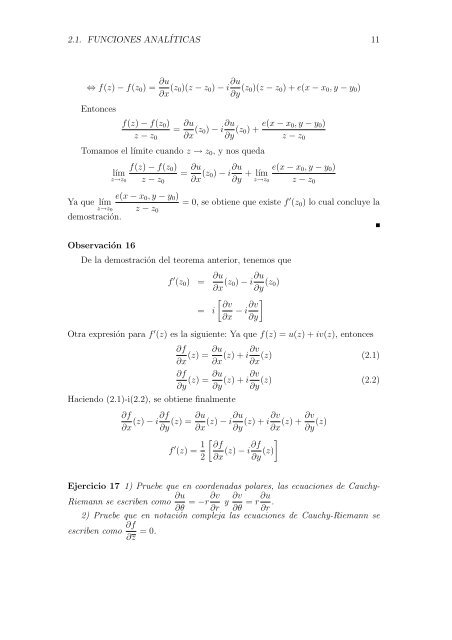
2.1. FUNCIONES ANALÍTICAS 11
⇔ f(z) − f(z0) = ∂u
∂x (z0)(z − z0) − i ∂u
∂y (z0)(z − z0) + e(x − x0, y − y0)
Entonces
f(z) − f(z0)
z − z0
= ∂u
∂x (z0) − i ∂u
∂y (z0) + e(x − x0, y − y0)
z − z0
Tomamos el límite cuando z → z0, y nos queda
f(z) − f(z0)
lím
z→z0 z − z0
e(x − x0, y − y0)
Ya que lím
z→z0 z − z0
demostración.
Observación 16
= ∂u
∂x (z0) − i ∂u e(x − x0, y − y0)
+ lím
∂y z→z0 z − z0
= 0, se obtiene que existe f ′ (z0) lo cual concluye la
De la demostración del teorema anterior, tenemos que
f ′ (z0) = ∂u
∂x (z0) − i ∂u
∂y (z0)
=
∂v
i − i∂v
∂x ∂y
Otra expresión para f ′ (z) es la siguiente: Ya que f(z) = u(z) + iv(z), entonces
Haciendo (2.1)-i(2.2), se obtiene finalmente
∂f
∂x
(z) − i∂f
∂y
∂f ∂u
(z) = (z) + i∂v (z)
∂x ∂x ∂x
(2.1)
∂f ∂u
(z) = (z) + i∂v (z)
∂y ∂y ∂y
(2.2)
∂u
∂v
(z) = (z) − i∂u (z) + i∂v (z) +
∂x ∂y ∂x ∂y (z)
f ′ (z) = 1
∂f
(z) − i∂f
2 ∂x ∂y (z)
Ejercicio 17 1) Pruebe que en coordenadas polares, las ecuaciones de Cauchy-
Riemann se escriben como ∂u ∂v ∂v ∂u
= −r y = r
∂θ ∂r ∂θ ∂r .
2) Pruebe que en notación compleja las ecuaciones de Cauchy-Riemann se
escriben como ∂f
= 0.
∂z