Design of an Automatic Control Algorithm for Energy-Efficient ...

8 System and functionality
integration
In this chapter the application of the optimiser algorithm for the car climate control will
be shown. The equations for the objectives found in Chapter 2 and the system (Chapter
3) have to be brought into a suitable form for the algorithm. User control and different
operating modes have to be integrated.
8.1 Objective implementation
The objectives are directly used as far as they can be expressed mathematically. The
results are used in the algorithm, as seen in Section 6.3.5, in two ways. On the one hand,
it is important if they exceed a limit. On the other hand, the weighted sum of all is used
if the limit comparison gives no winner. In order to make the weight designation and the
objective comparison easier it is advantageous to have a common maximum and minimum
objective result. This avoids that one objective becomes too dominant. The minimum is
set to zero, while for the maximum a parameter ���� is used.
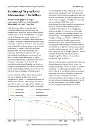
8.1.1 Windscreen fogging affinity
The basic equations to estimate the fogging affinity are given in Section 2.1. The finding
of the minimum, however, is not suited for a control application. The distance calculated
in equation 2.3 will be replaced by an estimation.
The idea is to approximate the closest point on the vapour saturation curve. This is
done via a local linearisation of this curve as seen in Figure 8.1. Starting from a measured
point � given through the water vapour pressure �� and a temperature � the points �