Design of an Automatic Control Algorithm for Energy-Efficient ...

ISSN 0280-5316 

ISRN LUTFD2/TFRT--5882--SE 

Design of an Energy-Efficient Climate 

Control Algorithm for Electric Cars 

Matthias Busl 

Department of Automatic Control 

Lund University 

June 2011

Lund University 

Department of Automatic Control 

Box 118 

SE-221 00 Lund Sweden 

Author(s) 

Matthias Busl 

Document name 

MASTER THESIS 

Date of issue 

June 2011 

Document Number 

ISRN LUTFD2/TFRT--5882--SE 

Supervisor 

Manuel Lorents Technische Universität München, 

Germany. 

Tore Hägglund Automatic Control Lund, Sweden 

(Examiner) 

Sponsoring organization 

Title and subtitle 

Design of an Energy-Efficient Climate Control Algorithm for Electric Cars (Design av en energieffektiv 

klimatregleringsmetod för elektriska bilar) 

Abstract 

A climatisation controller for a car with multiple objectives is developed, implemented 

and tested in simulations. The design focuses on electric cars and their specific 

characteristics. In this context the goal has been to fulfil common comfort and safety 

standards while having a low energy consumption. The main idea of the control in order 

to achieve this is to use a simplified model predictive control scheme to find the best 

compromise between those objectives. A special evolutionary algorithm and a simplified 

system model are developed for this purpose. Another feature of the control design is 

adaption of disturbance terms in this model based on their estimation. As interface to 

the hardware a second controller is introduced. The approach has been implemented for 

the electric car MUTE which is currently developed at the TU München. This 

implementation was verified to work with the available hardware and tested using a 

thermal car interior simulation model. 

Keywords 

Classification system and/or index terms (if any) 

Supplementary bibliographical information 

ISSN and key title 

0280-5316 

Language 

English 

Security classification 

Number of pages 

184 

http://www.control.lth.se/publications/ 

Recipient’s notes 

ISBN

Diploma thesis subject 

Problem statement: 

The more efficient car engines become, the more important the consumption of other 

power train elements gets. This becomes visible in the case of the electric car, where the 

power necessary for heating and cooling can exceed the drive power. Because there is no 

sufficient source of waste heat available, especially for the heating, the range of the car can 

be drastically reduced with an electrically powered heater. Therefore, countermeasures 

have to be taken in order to reduce the energy need and use as little electric energy as 

possible. Amongst others, these goals raise new questions in (automatic) control. 

Task: 

In the diploma thesis a control and an automatic control for the heating system of the 

car developed in the MUTE project should be designed. This system contains a liquid 

fuel heater and a heating, ventilating and air conditioning (HVAC) unit for air distribu- 

tion. Control and automatic control should provide the following functionality through 

automatic programs and options chosen by hand: 

• Heating (Automatic and manual mode) 

• Preconditioning of the passenger compartment and of the battery 

• Recirculating air control 

• Defrost mode 

The energy demand can be considerably reduced through an increased percentage of re- 

circulated air in the passenger compartment. The tendency of window fogging, which is 

measured with humidity and temperature sensors, should be added as control variable. 

The functionality, the control and the activation of the actuators should be tested with 

a test carrier. Sensors, actors and the developed control algorithm should then be imple- 

mented in the MUTE prototype. This has to be done in coordination with the institute for 

automotive engineering at the TUM, due to interfaces that have to be defined accurately. 

In a further step the integration of a heat pump as heat source/sink for the climatisation 

should be investigated on a simulation basis. The developed control algorithm should on 

the one hand take the dynamics and output limits of the heat pump into account and on 

the other drive the heating/cooling system towards its energetic optimal working point.

Abstract i 

Abstract 

A climatisation controller for a car with multiple objectives is developed, implemented and 

tested in simulations. The design focuses on electric cars and their specific characteristics. 

In this context the goal has been to fulfil common comfort and safety standards while 

having a low energy consumption. The main idea of the control in order to achieve this is to 

use a simplified model predictive control scheme to find the best compromise between those 

objectives. A special evolutionary algorithm and a simplified system model are developed 

for this purpose. Another feature of the control design is adaption of disturbance terms 

in this model based on their estimation. As interface to the hardware a second controller 

is introduced. The approach has been implemented for the electric car MUTE which is 

currently developed at the TU München. This implementation was verified to work with 

the available hardware and tested using a thermal car interior simulation model. 

Kurzfassung 

Ein Regelalgorithmus für eine Fahrzeugklimatisierung mit mehreren Zielvorgaben ist ent- 

wickelt, umgesetzt und durch Simulation getestet worden. Das Hauptaugenmerk lag dabei 

auf elektrisch angetriebenen Autos und ihren speziellen Eigenschaften. In diesem Kontext 

war das Ziel, allgemeine Anforderungen an Komfort und Sicherheit zu erfüllen und da- 

bei möglichst wenig Energie zu verbrauchen. Die Hauptidee, um dies mit einer Regelung 

zu erreichen, ist der Einsatz einer vereinfachten Form der model predictive control, um 

den besten Kompromiss zwischen den Regelungszielen zu finden. Dafür ist ein spezieller 

evolutionärer Algorithmus und ein vereinfachtes Model des zu regelnden Systems entwi- 

ckelt worden. Ein weiterer Bestandteil des Reglerdesigns ist die Anpassung der Modell- 

abweichungen durch eine Abschätzung. Als Schnittstelle zur Hardware wird ein weiterer 

Regler benutzt. Der Regelungsansatz ist für das Elektro-Auto MUTE, das zur Zeit an 

der TU München entwickelt wird, umgesetzt worden. Das Programm arbeitet in einem 

Teststand bereits mit der Hardware zusammen und ist mit einer Simulation des Fahrzeug- 

Innenraums getestet worden.

Acknowledgements ii 

Acknowledgements 

I would like to thank my supervisors, Manuel Lorenz and Leonhardt Hörth, for giving 

me the chance to work on this interesting and interdisciplinary topic and for their 

support. I am also very grateful to Tore Häggelund, who was willing to be my 

“examinator” without having had much information about the subject of this thesis. 

Many thanks as well to the creators and contributors of the open source community, 

especially Arch Linux, Gnome, LaTex, JLaTexEditor and gnuplot. Without this 

software this thesis would not be the same. 

I want to thank my parents for their love and their concerns and my sisters for the 

joyful time spent so far. 

In addition, I like to thank my friends, especially Desiderius for trying to fix my English 

and Zoe for calling if I did not. Special thanks to Regina for listening to my car climate 

control explanations and the support (not only the cooking). mpfh.

Contents 

Abstract i 

Acknowledgements ii 

Nomenclature ix 

1 Introduction 1 

1.1 A brief history of car climate control ..................... 1 

1.2 Trends in car climate control .......................... 2 

1.3 Overview of this work ............................. 3 

2 Control objectives 4 

2.1 Windscreen defogging .............................. 5 

2.2 Comfort ..................................... 7 

2.2.1 Thermal comfort ............................ 7 

2.2.2 Inhomogeneous climate ......................... 9 

2.2.3 Air humidity . . ............................ 10 

2.2.4 Air quality ................................ 11 

2.3 Power consumption ............................... 12 

2.4 Influence on other components ......................... 15 

3 System description 16 

3.1 The car cabin system .............................. 16 

3.1.1 Cabin air temperature ......................... 16 

3.1.2 Water mass in the cabin air ...................... 19 

3.1.3 Carbon dioxide concentration ..................... 20

Acknowledgements iv 

3.1.4 Windscreen temperature ........................ 21 

3.1.5 Time constant considerations ..................... 25 

3.2 TheHVAC-unit................................. 26 

3.2.1 The fan ................................. 27 

3.2.2 Air mixing ................................ 29 

3.2.3 Dehumidification ............................ 29 

3.2.4 Heating ................................. 30 

3.2.5 The flaps ................................ 31 

3.3 Theheatpump ................................. 32 

3.3.1 Energy efficiency ............................ 34 

3.3.2 Heat exchanger icing .......................... 35 

4 Control strategy 37 

4.1 Existing control structures ........................... 37 

4.2 Climate control in buildings .......................... 38 

4.3 The control concept ............................... 39 

4.4 The disturbance estimator ........................... 41 

4.5 The working point optimiser .......................... 42 

4.6 The HVAC-system control ........................... 44 

5 The disturbance estimator 46 

5.1 Estimation of disturbances ........................... 46 

5.2 Simulation as replacement for sensors ..................... 47 

6 The optimiser: an evolutionary algorithm approach 49 

6.1 The optimal control problem .......................... 49 

6.2 Algorithm selection ............................... 51 

6.2.1 Selection criteria ............................ 51 

6.2.2 Gradient based algorithms ....................... 52 

6.2.3 Evolutionary algorithms ........................ 52 

6.3 Design of an incremental micro evolutionary algorithm ........... 55 

6.3.1 Overview of IMEA ........................... 55

Acknowledgements v 

6.3.2 Design variable coding ......................... 57 

6.3.3 Generation of the initial population .................. 57 

6.3.4 System simulation and objective evaluation .............. 58 

6.3.5 Ranking and constraint handling ................... 58 

6.3.6 Elitism and base population . . .................... 61 

6.3.7 Selection ................................. 62 

6.3.8 Recombination and mutation ..................... 63 

6.3.9 Replacement ............................... 65 

6.3.10 Control signal choosing ......................... 65 

6.3.11 Final thoughts on the algorithm .................... 66 

7 The HVAC-system controller 68 

7.1 Temperature and humidity control ...................... 68 

7.2 Heat pump control ............................... 70 

7.3 Fan control ................................... 70 

7.4 Flap control . . ................................. 70 

7.5 Cold air prevention system ........................... 71 

8 System and functionality integration 72 

8.1 Objective implementation ........................... 72 

8.1.1 Windscreen fogging affinity ...................... 72 

8.1.2 Thermal comfort ............................ 75 

8.1.3 Air speed comfort ............................ 79 

8.1.4 Humidity comfort ............................ 81 

8.1.5 Air quality ................................ 82 

8.1.6 Power consumption ........................... 84 

8.1.7 Component thermal management ................... 84 

8.2 Constraint formulation ............................. 84 

8.2.1 Integration as boundaries ....................... 87 

8.2.2 Integration as objectives ........................ 87 

8.3 Parameters for the objectives ......................... 88 

8.4 User control ................................... 89

Acknowledgements vi 

8.5 System simulation ................................ 91 

8.6 Optimiser algorithm parameters ........................ 91 

8.6.1 Population size ............................. 91 

8.6.2 Other settings .............................. 92 

9 The MUTE project 94 

9.1 The electric car MUTE ............................. 94 

9.2 Climatisation in the MUTE car ........................ 95 

10 Hardware and characteristics of the MUTE prototype 97 

10.1 The car interior ................................. 97 

10.2 The HVAC-unit ................................. 99 

10.3 The heating unit ................................101 

10.4 The sensors ...................................103 

10.5 Other available information ..........................104 

10.6 The user interface ................................106 

10.7 Computer and electrics . . . ..........................107 

10.8 Parameterisation for the MUTE car......................108 

11 Matlab implementation 109 

11.1 Model structure .................................109 

11.2 Automatic mode ................................111 

11.3 Programming ..................................114 

11.4 Real-time requirements . . . ..........................115 

12 Controller evaluation 116 

12.1 Hardware-in-the-loop test ...........................116 

12.2 Optimiser performance evaluation .......................117 

12.3 Simulation test layout .............................119 

12.4 The test cases ..................................120 

12.5 Simulation results ................................123 

12.6 Stability and robustness ............................126

Acknowledgements vii 

13 Conclusion 128 

13.1 Extension for full car air conditioning .....................128 

13.2 Possible improvements .............................129 

13.3 Outlook .....................................129 

Bibliography 131 

Appendices 

A Constants and material properties 136 

A.1 Tabular material constants ...........................136 

A.2 Miscellaneous material constants .......................136 

B In- and outputs 137 

B.1 Controller inputs ................................138 

B.2 Controller outputs ...............................140 

B.3 Error codes ...................................141 

C Simulation parameters 142 

C.1 Hardware data and system parameters ....................143 

C.2 Controller settings ...............................145 

C.2.1 Design variable related settings ....................145 

C.2.2 Objective related settings .......................145 

C.3 Disturbance estimator settings .........................147 

C.4 Optimiser settings ................................148 

C.5 Test case parameters ..............................149 

D Additional simulation results 150 

D.1 Heat-up test case ................................150 

D.1.1 No recirculation .............................150 

D.1.2 Changed user settings .........................151 

D.2 Cool-down test case ...............................151 

E Optimiser code 152

Nomenclature viii 

Nomenclature 

Symbols 

Symbol Unit Description 

� [� � ] Area 

�� [-] Biot number 

��, �� , � [ � 

��¡� ] Heat capacity 

� [-] Pressure coefficient, constant 

� [�] Distance, thickness 

� [�] Diameter 

� [-] Euler’s number 

� [�] Internal energy 

� [-] Ratio 

� [ � 

�� ¡� ] Convective heat transfer coefficient 

� [ �� 

�� ] Specific enthalpy 

� [ � 

�¡� ] Thermal conductivity 

� [-] Gain 

�� [�] Length 

� [��] Mass 

�� [ �� 

� ] Mass flow 

� [��] 1 Metabolism 

� [��] Pressure 

� [�] Power 

�� [ � 

�� ] Heat flux 

� [�] Heat energy 

�� [�] Heat transfer rate 

� �� [��] 2 Clothes insulation, thermal resistance per area 

� [ �� ¡� 

� ] Thermal resistance 

1 � �� , sitting calm [1] 

2 � �� ¡� 

� , business clothes [1] 

Continued on the next page

Nomenclature ix 


� [�] Time 

� [℃] Temperature 

� [ �] 

Speed 

� 

� [� � ] Volume 

� [-] Weight 

� [��] 1 External work 

� [�] Energy 

� [�] Variable distance 

�� [-] Variables 

� � 

� �� 

Greek symbols 

[ �� 

] �� 

Absolute humidity 

[ �� ] �� 

Absolute carbon dioxide concentration 


� [°] Angle 

� [-] Transmittance 

� [℃] Distance to water vapour saturation 

� [-] Air fraction passing a flap 

� [�] Time constant, time 

� [%] Relative humidity

Nomenclature x 

Other symbols 

Symbol Description 

� Objective values of an individual � 

� Objective values of an individual � 

� Function 

��, �� Fitness, here: weighted sum 

� Constraint function 

�, � Limits for the objectives 

� Trajectory cost 

�� Vector with lower bounds for the design variables 

� Number 

�, � (Panic) ordering 

�, � Priorities for the objectives 

�� Selection probability 

� Random value 

� � 

Exploration factor 

�, � Control output 

� Set of allowed control outputs 

�� Vector with upper bounds for the design variables 

�, � Weights for the objectives 

�, � System state 

� Set of allowed system states 

� �� 

Exploration factor in-/decrement 

�� Sample time 

� �� 

� �� 

Elite selection threshold percentage 

Maximum allowed distances from the old control value 

�, � Standard deviation 

�, � Final cost, objective (function) 

�� symbols indicate vectors.

Nomenclature xi 

Subscripts 

Subscript Description 

act Actual, measured 

air Air 

amb Ambient, the air outside the car 

base Base individuals 

c Child/children 

cab Car cabin 

cl Clothes 

defrost Defrost air outlets 

elite Elite individuals 

eval Evaluations 

face Face air outlets 

foot Foot air outlets 

gen Generation 

h Height 

horizon Prediction time, horizon 

in In or into the car cabin 

i, j, k ,n Numbering 

max Maximum 

min Minimum 

obj Objective(s) 

out Outside or out of the car cabin 

pas Passenger 

par Parent 

pop Population 

pow Power 

r (Solar) radiation 

random Random immigrants 

Continued on the next page

Nomenclature xii 

Subscript Description 

recirc Recirculation 

sat Saturated 

sun Sun 

tot Total 

v (Water) vapour 

w Water 

ws Windscreen

Nomenclature xiii 

Abbreviations 

Abbreviation Description 

BIBO Bounded-Input Bounded-Output 

CAD Computer Aided Design 

CAN Controller-Area-Network 

CFRP Carbon Fiber Reinforced Plastic 

CO2 

Carbon dioxide 

COP Coefficient Of Performance 

EA Evolutionary Algorithm 

GAME Genetic Algorithm for Multicriteria Engineering 

HVAC Heating, Ventilating, and Air Conditioning 

IMEA Incremental Multi-objective Evolutionary Algorithm 

ISO International Organisation for Standardisation 

LTI Linear Time Invariant (system) 

MPC Model Predictive Control 

NSGA-II Non-dominated Sorting Genetic Algorithm II 

OEL Occupational Exposure Limits 

PID Proportional–Integral–Derivative (controller) 

PMV Predicted Mean Vote 

PPD Predicted Percentage of Dissatisfied 

PTC Positive temperature coefficient; materials used for electric 

heating 

PWM Pulse Width Modulation 

rH Relative Humidity 

SoC System-On-a-Chip 

SQP Sequential Quadratic Programming 

TCO Total Cost of Ownership

1 Introduction 

Energy consumption takes a growing importance in industry and consumer products, as a 

risk for the world climate, but also as a cost factor and selling point. The car industry is 

on the run for the “green” car, driven by growing international standards and restrictions 

for emissions and consumers demands. On the horizon a new type, the electric car, can 

be seen. 

The climatisation of these vehicles becomes a difficult task. On the one hand the 

power consumption should decrease, on the other hand a replacement for the lower “waste- 

heat” of motors (especially when using electric ones) needs to be available. In order to 

solve this dilemma, car climatisation becomes a field of innovative concepts offering new 

possibilities of (automatic) climate control. 

1.1 A brief history of car climate control 

When the first cars got faster they needed a closed car body. This enclosed space had 

to be ventilated in order to provide the passengers with fresh air. The first ventilation 

systems - windows that could be opened - were controlled by hand. The heaters that 

became standard in the fifties [1] were operated by the driver as well via a turning knob 

or other elements. 

This did not change even when the first air conditioning providing cooling and 

dehumidification (without the option of air humidification) was introduced into the mass 

market (first 1954). The mechanics behind the knobs were changed to potentiometers and 

motors from the 1970s onward (seen in Figure 1.1), but today the “thermal control loop” 

is still often closed by the human in the car: The driver adjusts the inlet-air settings in 

order to achieve a comfortable climate.


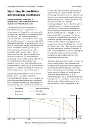
Figure 1.1: The development of climate control units. [2] 

In 1964 the first system for an automatic controlled cabin temperature was brought 

onto the market by Cadillac. Having been an optional feature for upper class cars regarded 

as a luxury in the beginning, an automatic “climate control” can now be ordered for almost 

every car. This is easily possible through the electrification mentioned before and the 

introduction of digital control (first 1975 by Rolls-Royce). Still what is called automatic 

climate control is in most cases only automatic temperature control. 

A climate control should also include humidity control if not other factors like the 

carbon dioxide concentration [3] and the air outlet distribution. Basic approaches are 

found for example in air quality sensors for automatically enabling air recirculation in 

order to prevent odours and exhaust gases from entering the cabin. However, increased 

passenger comfort still is the main reason for these systems being integrated into cars. 

1.2 Trends in car climate control 

There are two trends that can be seen in automatic climate control in cars. 

First there is a trend towards more complexity in the equipment. New sensors 

allow better automatic control, for example an improved solar sensor [4] and the already 

mentioned CO2 sensor. The use of decoupled electronic operated compressors (as in 

the Toyota Prius [5]) and humidity sensors allows better use of recirculation and better


adjustment of the compressors working point. These new “tools” make it possible to 

increase safety through fogging-prevention and providing better thermal comfort while 

using less electricity. 

The second trend is a constant pricing pressure. This is nothing in car industry, 

but leads to the result that only such features are integrated into a new model which give 

a benefit to the customer that she or he is willing to pay for or are cheaper. Therefore, 

the possibilities described in the paragraph above will mostly be offered as an expensive 

option or not used at all in combustion cars. 

In an electric car, however, these new developments give a benefit that is very 

valuable: extended range. Their integration into hybrid cars has prove that they are 

worth the price. 

1.3 Overview of this work 

In Chapter 2 the objectives for a car climate control will be shown in detail. Chapter 3 

presents the subject of the control, the car cabin system and the HVAC-hardware, with 

simple system equations. Then, an automatic climate control strategy is presented in 

Chapter 4. Its components and the applied algorithms are described in Chapters 5, 6 and 

7. How the control objectives, the system and the required functionality are integrated 

into this control concept is shown in Chapter 8. 

The designed algorithm is implemented in Matlab for the use in the electric car 

MUTE. The concept of MUTE and and its climatisation strategy are found in Chapter 9. 

The car’s material, actors, sensors and processing hardware are explained in the following 

Chapter 10. Chapter 11 covers the implementation of the presented solution in Matlab 

and Simulink. Results of this working control program are presented in Chapter 12, as 

far as they could be obtained without an existing car in the hardware-in-the-loop test 

rig and in simulations. The thesis concludes with a summary and an outlook at possible 

improvements.

2 Control objectives 

For an electric car energy saving is especially important. Accordingly, the power con- 

sumption should be minimised by the controller. However, other objectives have to be 

taken into account, too. 

The cooling/heating system may also be used for tempering car components as 

power electronics and the motor. Their thermal working point has then to be taken care 

of, too. The main reason, however, for advanced climate control in cars still is comfort - 

as stated in the last chapter. More fundamentally, it has to provide safety. 

A closer look will be taken in this chapter at the following four general objectives: 

• maximising safety 

• maximising comfort 

• minimising power consumption 

• optimising the (thermal) working point of components 

The reduced power consumption is often opposed to the other objectives although 

it may match comfort wishes like low noise. For example, recirculating air reduces the 

required heating (or cooling) power, but it leads to faster fogging and impairs the air 

quality. 

This is only accepted to a certain degree by the passengers. Of course, a high 

thermal comfort is an important sales argument for a car, but it is also connected to 

safety. A good automatic operation with little need to adjust leads to less distraction, 

and a driver who is in a comfortable (thermal) environment can focus better on the traffic 

[1]. However, the most important safety aspect is free view trough the windscreen (i.e. 

no fogging or icing).


2.1 Windscreen defogging 

Fogging occurs when the air at the windscreen is saturated with water. Water precipitates 

on the glass and limits the view. The amount of water in the air leading to condensation 

is dependent on the air temperature. The saturation vapour pressure (maximum partial 

vapour pressure) can be well approximated within the relevant limits for a car by the 

following equation taken from DIN 4108-5 [6]. The resulting curve is shown in Figure 2.1. 

� �� ¡ 

� �� 

� 

� � � 

� 

�� ℃ 

Water vapour saturation pressure [Pa] 

� Water vapour temperature [℃] 

� �, � �, � � 

Constants 

Table 2.1: Constants used in equation 2.1 for the different temperature ranges. [6] 

Phase Temperature range � � [Pa] � � � � 

Ice 4.689 1.486 12.30 

Water 0 ℃ - 30 ℃ 288.68 1.098 8.02 

(2.1) 

There exist several solutions to detect fogging. Some are based on optic effects 

(infrared or a camera). The majority of implementations use a humidity sensor coupled 

with temperature measurements on the (glass) surface. The following will focus on a 

system where the absolute humidity in the cabin as well as the windscreen temperature 

is known (i.e. measured) . With this data the position in Figure 2.1 can be determined 

and a “fogging risk” can be calculated. In this way an impairment of the driver’s vision 

can be avoided. 

Relative humidity is not a good indicator to determine how close to fogging the 

conditions are since it depends a lot on the temperature. In the paper Prediction of Water 

Vapor Condensation on Automobile Windscreens [6] C. Gühmann defines an absolute 

distance of a point to the saturation curve in the temperature-water vapour pressure 

diagram. To compensate for the different units of both axes in the graph a factor is


�� 

�� 

�� 

�� 

�� 

�� 

�� 

�� 

�� 

�� 

� �� 

�� 

�� 

�� 

�� 

�� 

�� 

�� 

�� 

�� 

�� 

Figure 2.1: Saturation vapour pressure curve and the fogging affinity �. 

required. This is achieved by taking the average slope of the saturation curve in the range 

from -20 to 30 ℃. 

�� ¡�� ¡� � �� ℃ ��℃� ��℃ ��℃ 

�� 

� 

(2.2) 

The distance � represents the affinity to condensate of a partial water vapour 

pressure � � on a windscreen with the temperature � �� and is then calculated by [6] 

� � �� 

�� 

�� 

�� 

� 

� (2.3) 

An example can be seen in Figure 2.1.


2.2 Comfort 

General influences on comfort by P.O. Fanger can be seen in Figure 2.2. The environmental 

factors are those of highest interest here since they can be influenced by the climatisation. 

The human and other factors differ between passengers. They need to be estimated the 

best possible or adjustable. Among the psychological factors, noise will not be taken into 

Figure 2.2: Influences on comfort as found by P. O. Fanger. [2] 

account since it can hardly be influenced by the climate control. Its main source in the 

HVAC-unit is the fan. This topic will mostly be addressed in the hardware development. 

The fan speed will also be regarded through the energy consumption objective. A quite 

important factor is odour in the sense of air quality since fresh air supply is the main 

reason for having a ventilation system in a car. 

2.2.1 Thermal comfort 

A well established calculation of thermal comfort is the one found by Fanger in the 1970s. 

It is also included in the ISO standard 7730 [7]. 

The method is based on a body’s heat balance equation: 

(2.4)


�� 

�� 

�� 

�� 

�� 

�� 

�� 

Internal heat production 

Heat loss due to water vapour diffusion through the skin 

Heat loss due to sweating 

Latent heat loss due to respiration 

Dry respiration heat loss 

Heat loss by radiation from the surface of the clothed body 

Heat loss by convection from the surface of the clothed body 

By combining this equation with experimental data a comfort index reaching from 

-3 (too cold) to +3 (too hot) has been found. The resulting figure is called Predicted 

Mean Vote (PMV). 

�� ¡ � �� (2.5) 

The expressions used in equation 2.5 can be stated as follows [8]: 

�� 

�� ¡ �� 

�� 

�� ¡ �� 

�� 

�� ¡ �� 

�� 

� �� 

� �� 

� �� 

� 

�� 

�� 

� 

�� 

�� 

�� for �� 


�� for � �� 

�� for � �� 

(2.6) 

(2.7)


� Metabolism [��] (�� 

�� , sitting calm) 

� External work [��] 

� � 

� �� 

� �� 

� �� 

� � 

� �� 

� �� 

� �� 

Water vapour pressure [��] 

Air temperature [℃] 

Ratio of the surface area of the clothed body to the surface area of the 

nude body [-] 

Surface temperature of the clothing [℃] 

Mean radiant temperature [℃] 

Convective heat transfer coefficient [ � 

�� ¡� ] 

Thermal resistance of clothing [��] (�� ¡� 

� ) 

Relative air velocity [ � 

� ] 

2.2.2 Inhomogeneous climate 

The model by Fanger was developed for stationary environmental conditions. It gives no 

means of including the influence of different temperatures and air flows on the body. 

A more complex approach is used in the ISO standard 14505-2 [9] by measuring 

temperatures of body parts. A comfort function chart found in these experiments is given 

for a winter and a summer case. It is found that a cooler temperature in the head area 

is desired, while warm feet lead to maximum comfort, especially with cooler ambient 

temperatures. This is opposed to the natural air layering where the warmer and lighter 

air is on top. 

Controlling this online would require a lot of sensors and actors. Therefore, this 

is usually implemented in hardware in a car HVAC-system. The air flow is optimised in 

such way that warm air is output through the foot and defrost outlets, while cooler air 

is going directly to the passenger. Manual adaption of the direct air flow temperature is 

sometimes implemented. Since this is related to the hardware, the temperature layering 

will not be regarded further in this work. 

The air flow itself can also cause discomfort. Higher air speed on the body leads to 

higher heat transfer coefficients and consequently to an intensified temperature sensation. 

The effect of moving air with ambient temperature is included in the comfort calculation 

in equation 2.6. Local air jets with a different temperature, however, as they occur in a


car, are not considered. They can be comfortable when the air from the outlet is warm 

but should be avoided when it is cold. A more detailed temperature dependent sensation 

chart by Teerhag (1986) [10] is shown in Figure 2.3. A formula to calculate the percentage 

Figure 2.3: Comfort in relation to air speed and its temperature as found by Teerhag 

(1986). [10] 

of dissatisfied persons by air flow is given in ISO 7730 [7] and illustrated in Figure 2.4. It 

is also noted that air speeds above should be avoided. However, no other influences 

(like radiation) which could lead to a comfortable feeling even at cooler or higher air flows 

are included in both charts . 

2.2.3 Air humidity 

Not only (felt) air temperature is influencing comfort. High humidity can lead to oppres- 

sive climate even if one is not feeling hot [1].Moisture is undesired since it supports the 

development of microorganisms. On the other hand very dry air can irritate the mucous 

membranes and the skin. In 1951, Leudsen and Freymark found a correlation for buildings 

shown in Figure 2.5. The recommendations made in DIN 1946-3 [11] to keep the relative 

humidity between 30% and 60% for comfort temperatures are also shown in this figure.


�� 

�� 

�� 

�� 

�� 

�� 

�� 

�� 

�� 

�� 

�� 

�� 

�� 

�� 

Figure 2.4: The percentage of dissatisfied people by air flow according to ISO 7730 [7] 

(turbulence = 40%). 

Another general proposed rule of thumb is to keep the absolute humidity below �� [1]. 

It can be seen that a large range of air humidity is acceptable. Influences on the 

felt temperature are already implemented in the equations 2.6. 

2.2.4 Air quality 

Apart from humidity the air in a car contains many other substances. In too high concen- 

trations most of them lead to unpleasant side effects. Particles like pollen can irritate the 

eyes and the mucous membranes. They are mostly filtered in the HVAC-system and will 

therefore not be taken into account. Gases in differing concentrations can lead to odour 

and - very undesirable in a car - impair concentrativeness [13]. 

The most important of these gases is carbon dioxide which is often used as an 

indicator for air quality and emitted by humans. A maximum concentration in a working 

environment or occupational exposure limit (OEL) is given by a value of �� (which 

equals �� or �� 

� � ) [1]. This level can be reached after 8 minutes in a standard 

�� 

�� 

�� 

�� 

�� 

�� 

�� 

�� 

�� 

��


�� 

�� 

�� 

�� 

�� 

�� 

�� 

�� 

�� 

�� 

�� 

�� 

�� 

�� 

�� 

�� 

Figure 2.5: Comfort in humid air as found in Leudsen and Freymark (1951) [12] and 

DIN 1946-3 [11]. 

car with four persons and without fresh air supply (e.g. in recirculation mode) [1]. 

Most of the other sources give a lower concentration as guideline value. A relation 

between the percentage of dissatisfied people and the CO2 level [14] is shown in Figure 

2.6. 

It is seen that at a level of �� above the outdoor carbon dioxide concentration 

(of around �� -�� ) nearly 20% percent of the people are dissatisfied. 

This causes no problem as long as only fresh air ventilation is used. With an 

increased use of recirculation though, the concentration can increase quite fast. Hence 

pure recirculation should be avoided. A minimum fresh air supply rate of �� 

� Person is 

advised to obtain an acceptable air quality [13]. 

2.3 Power consumption 

An HVAC-system has three main power consumers: the cooling unit, the heating unit and 

the ventilation. The remaining electric components, like motors for the flaps or sensors,


Figure 2.6: The perceived air quality (% dissatisfied) as a function of the carbon dioxide 

concentration. [14] 

do not take much power. 

The fan is spinning nearly all the time to provide the passengers with fresh air. 

This is necessary as seen in Section 2.2.4. Depending on the model its power consumption 

can be as high as �� [1]. Although this will be needed rarely. An average consumption 

below �� is realistic for normal car. 

A typical cooling power in a car is around �� [2]. The installed and maximum 

power may be higher. In the refrigeration circuit the only powered unit is the compressor. 

The refrigerant is compressed and enters the condenser to transfer heat to the ambient air. 

It is then liquefied and expanded into the evaporator cooling the inlet-air. The vaporised 

gas returns to the compressor and the cycle starts again. In this way heat is transferred 

from the interior to the outside and the car is cooled. The compressor only consumes the 

electric power to compress the gas. This corresponds to around 33%-50% of the cooling 

power. The energy is mostly taken mechanically from the (fuel-)engine and is replaced 

by a separate motor in an electric car. 

A typical heating power for a car is around �� and thus of the same magnitude 

as the cooling power [2]. In today’s fuel-run cars most of this is provided by the engines’ 

waste heat. Only if this it not sufficient, electrically heated PTC-elements are used. 

Taking away the combustion process as main heat source other solutions have to be found 

for the electric car. Using electricity directly with PTC-elements is not economical. Heat


pumps or fuel heaters are more efficient options when it comes to power consumption. 

A fuel heater only needs electric power for the ignition process and for its fan. 

During the ignition around �� can be drawn from the power supply. Once started 

the consumption is quite low. The fuel consumption for such small heaters are around 

� �� ¡�� . However, a reservoir for the fuel has to be provided. 

A heat pump is basically working like a refrigeration circuit, but with the possibility 

to heat the passenger compartment as well. As heat sources not only the ambient air can 

be used, but also internal components like the battery pack or the electric motor. A 

detailed description of the functioning is found in section 3.3. The advantage of this 

solution is that it does not need a separate energy source like fuel. In addition, nowadays’ 

standard of heating and cooling (and thereby dehumidification) can be combined in one 

system. On the other hand, the electric energy consumption will be higher than a fuel 

based solution. The power demand is dependent on the components (e.g. the compressor) 

and on the temperature level of the heat source/sink and the desired output temperature. 

One critical point concerning the use of a heat pump in a car is icing of the front heat 

exchanger (evaporator) when heating in winter. This leads to a dramatically decreased 

efficiency down to a point where the refrigerant circuit does not work anymore. 

Typically there are no sensors measuring the power consumption of the components, 

but since they are directly controlled the current can be estimated. The components’ 

consumption has to be measured once and then these values are used. 

When the energy is consumed is also an important fact in an electric car. There 

might be situations, when it is good to consume as much as possible, for example when 

the battery is fully charged, but the car is recuperating. On the other hand when the 

car is short on electric power or the connection to the high voltage system fails, only the 

current absolutely necessary may be drawn. In general the power consumption should be 

minimised while providing a maximum comfort, but this is dependent on the cars energy 

overall situation.


2.4 Influence on other components 

Components like the battery, the power electronics and/or the electric machine can be 

used as heat sources or sinks with a heat pump as mentioned before. When doing so the 

influences on these parts have to be taken into account. 

The battery, for example, needs a certain temperature to be able to deliver high 

power. Above a certain temperature, though, gases will evaporate and lead to possible 

failure or even safety risks up to inflammation and explosion. For a prolonged lifetime, 

which is of interest since the battery is most expensive part of an electric car at the 

moment, an optimal temperature frame exists. For the electrics it might be advantageous 

to be as cold as possible, but below a certain level mechanics (lubricant viscosity) will 

oppose. 

The component manufacturers specify a temperature range for an optimal func- 

tioning. The thermal management system takes the responsibility for not exceeding these 

limits.

3 System description 

In order to understand how the involved systems are working and interacting physical 

models are made use of. These are kept as simple as possible to find out about the (main) 

influences. The use in the controller requires as well models that are fast to calculate. 

For this reason, 3D fluid dynamics simulations will not be treated here. The following 

equations will be one-dimensional and will not describe details of disturbances which are 

very hard to measure online (as e.g. air leakage). 

3.1 The car cabin system 

In the car cabin system, the air in the car and the windscreen will be considered. Four 

quantities or states were identified to be relevant for the objectives found in Chapter 2: Air 

temperature, absolute humidity, carbon dioxide concentration as well as the windscreen 

surface temperature for the fog detection. 

3.1.1 Cabin air temperature 

In a car we have first the desired and controlled air flow from the HVAC-unit. The amount 

of air blown into the cabin will also leave it (in a steady state). These two heat flows 

are denoted by �� and ��. The sources not connected to air flow are the heat transfer 

through the car body ( ��) and the solar radiation ( ��). These two influences can in 

most cases be regarded as static or slowly changing over one trip. Transient heat sources 

are the thermal masses in a car. For heating a car in the winter a lot of energy is used 

to heat-up the seats, the car body and other parts. This heat source (or sink) is named 

��. Other influences on the temperature in the car are often hard to quantify and will 

be summed into ��. This can be air leakage, the passengers in the car, electronics


or heat coming from the engine. There are additional disturbances like open windows 

or doors which are important to the air temperature. They are also covered by “others” 

since they are unpredictable and hard to compensate for. Figure 3.1 shows all the heat 

flows and approximately where they occur in the car. 

If the sum of these influence is unbalanced (i.e. ), a change in the thermal 

energy of the air in the cabin ( ) occurs, giving a . 

� �� 

�� 

�� 

�� 

�� 

� �� 

Figure 3.1: Heat balance in a car. 

The resulting basic heat balance equation reads: 

�� 

(3.1) 

H. Großmann [1] gives formulas for most of the heat flows. They are extended and a


parameter for the fraction of recirculated air, ��, is introduced. 

�� ¡ �� ¡ �� 

�� 

�� ¡ �� 

�� ¡ �� ¡ �� ¡ �� 

�� 

�� 

¡ � � �� ¡ �� 

�� ¡ �� ¡ �� ¡ �� 

�� Air mass in the cabin [��] 

�� 

Specific heat capacity of the air at constant volume [ �� 

��¡� ] 

�� Air mass flow through the car [ �� 

� ] 

Percentage of �� being recirculated [�] 

�� 

�� 

� �� 

� �� 

Specific heat capacity of the air at constant pressure [ �� 

��¡� ] 

Heat transfer through the car body [ � 

� ] 

�� ¡ �� Heat capacity of the parts of the car interior and body [ �� 

� ] 

� Time [�] 

�� Thermal power of the HVAC-system heater [�] 

�� 

�� 

�� 

�� 

�� 

�� 

(Mean) temperature of the air in the cabin [℃] 

Temperature of the air leaving the cabin [℃] 

Window area � [� � ] 

Angle between surface normal of � and direction to the sun [°] 

Transmittance of � [-] 

Sun intensity [ � 

� � ] 

(3.2) 

Interior parts and the air are assumed to have the same temperature here. This 

is not correct, however, since the sun influence heats up the interior much more than the 

air. If this was considered, a more complicated model will be required introducing the 

(surface) temperature of the interior as a new state. 

The outlet temperature �� will be simplified set equal to ��. Different ap- 

proaches to estimate this temperature [1] are suggested but they are only valid without 

recirculating air and for standard car layouts. The heat transfer of the car � �� 

� �� 

can be


calculated by summing up the contributions of all the cabin parts [1]: 

�� 

�� 

� 

�� 

�� 

� 

�� 

� �� 

� 

�� 

� 

�� (3.3) 

While the thermal conductivity � and the material thickness � and area � are usually 

known and constant, the convection heat transfer coefficients on the outside, ��, and 

inside the cabin, ��, depend on the air speed. Großmann gives approximations for 

these correlations: �� 

��, �� 

�� 

equation: 

The temperature of the air blown into the cabin can be expressed with the following 

�� ¡ 

� 

�� ¡ �� 

� �� ¡ �� ¡ �� (3.4) 

Combining equations 3.1, 3.2 and 3.4, a differential equation for an estimation of 

the mean cabin temperature can be given. 

�� 

� 

�� ¡ �� ¡ �� ¡ 

� 

�� ¡ �� ¡ �� 

�� 

3.1.2 Water mass in the cabin air 

�� 

¡ �� 

�� 

�� 

� (3.5) 

Water in the cabin has two sources. One is the incoming (moist) air. The other are the 

passengers with their respiration, sweat as well as other humidity in the clothes and shoes. 

Water leaves the car through the air outlet or is separated at the evaporator. 

A basic water equation is found at Großmann [1]. It is however only applicable in 

a steady context and does not implement a recirculated air percentage ��. Therefore, 

it is modified in the following: 

�� 

�� (3.6)


�� Water mass in the cabin air [��] 

�� 

�� 

�� 

Water mass flow in the incoming air [ �� 

� ] 

Water mass flow leaving the car [ �� 

� ] 

Water mass flow produced by the passengers [ �� 

� ] 

�� Water mass flow condensed at the evaporator [ �� 

� ] 

The water emitted by a human is dependent on many environmental and physio- 

logical factors (cf. Section 2.2.1). A value of �� 

� 

per person [1] can be assumed 

for an activity between � and � �� [14].The amount of condensed water is regarded in 

Section 3.2. For the other components equations can be given: 

�� ¡ �� 

�� ¡ �� ¡ �� 

�� ¡ �� ¡ �� 

�� Absolute humidity of the cabin air [ �� 

] 

�� 

�� Absolute humidity of the ambient air [ �� 

] 

�� Dry air mass flow into the car [ �� 

� ] 

�� 

(3.7) 

A complete differential equation for the absolute humidity in the cabin air is ob- 

tained by combining the relations found in equations 3.6 and 3.7. 

�� 

�� 

� 

� ¡ �� ¡ �� ¡ �� 

�� 

(3.8) 

3.1.3 Carbon dioxide concentration 

A basic equation for concentrations of gases is given by Temming (1984) [1]. This is 

modified and the recirculation introduced with ��. As result a differential equation to 

quantify the CO2 concentration is obtained. 

�� 

�� 

� 

� 

¡ �� ¡ �� ¡ �� (3.9) 

��


�� Absolute CO2 concentration in the cabin air [ �� 

�� ] 

�� Absolute CO2 concentration in the ambient air [ �� 

�� ] 

�� 

�� 

� 

CO2 production rate (by passengers) [ � 

� ] 

The carbon dioxide emission of a person is given as �� 

for an activity of �-�� and �� 

3.1.4 Windscreen temperature 

� 

� 

[1]. Different values of 

for � �� can also be found [14]. 

The temperature at the inner side of the windscreen is of interest since fogging usually 

occurs here. Even if it is not equal on the whole surface, a mean value allows to estimate 

a temperature at least for the important middle part. In Figure 3.2 an overview of the 

� �� 

�� 

� �� 

� �� 

� �� 

� �� 

� �� 

� �� 

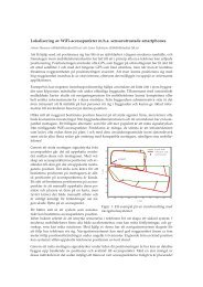
Figure 3.2: A schematic drawing of the heat transfer at the windscreen. 

influences and the heat transfer is shown. On the outer side ambient air flows over the 

glass depending on the car speed. On the inner side temperature and air speed are 

governed by the air coming from the defrost outlets. Finally, other influences like sun or 

rain contribute to the windscreen temperature � ��. 

Heat transfer coefficients 

The convection heat transfer coefficients � �� and � �� depend on the temperatures 

and the flow conditions. A forced convection is assumed in the following. This corresponds 

� ��


to a driving car and air blowing out of the defrost outlets. 

Accurate values are hard to calculate since flow conditions change with speed, wind 

and weather. Therefore, a simple approximation [1] of the coefficients for a longitudinal 

flow on a plate will be used: 

� 

�� ¡ �� for �� 

� � 

�� 

� 

� 

�� ¡ � �� 


� 

� Convection heat transfer coefficient [ � 

�� ¡� ] 

�� Air speed [ � 

� ] 

(3.10) 

To calculate the coefficient on the outside of the windscreen, ��, the car speed 

has to be corrected with a pressure coefficient �� in order to obtain the air speed. 

�� ¡ �� (3.11) 

�� Pressure coefficient [-] 

�� 

Car speed [ � 

� ] 

An average �� can be determined with experiments for a real car, but the true 

value cannot be given since it will be dependent on environmental influences like wind 

and rain. For a rough estimation it will be approximated by ��, a value obtained in a 

wind tunnel by the Modine Europe GmbH [15]. 

At the interior the air from the defrost outlets is blown onto the windscreen. The 

jet widens and the gets slower. As an estimation of the air speed the maximum velocity 

of a plane wall jet is taken [16]: 

� �� 

�� ¡ ¡ �� 

� 

� Defrost nozzle size (see Figure 3.3) [�] 

� Distance from the nozzle [�] 

(3.12) 

�� Air speed at the outlet [ � 

� ] 

The defrost nozzle size (��) is typically around ��. As distance from the


� 

� � 

�� 

� �� 

Figure 3.3: Configuration and nomenclature for the plane wall jet. 

outlet half the windscreen height � �� is taken since this is the area of interest. 

� �� ¡ 

� � ¡ �� 

� �� 

� �� 

¡ � �� 

(3.13) 

� �� can be estimated by dividing the air volume flow by the defrost outlet area. 

The air speeds obtained by this equation fit well with the magnitude of 2 � 

� 

example [1]. 

Differential equation for the temperature 

found in an 

The temperature of the windscreen glass will be assumed to be approximately equal. This 

is permissible if the Biot number �� ¡� 

�� . 

�� 

� ��. A calculation with typical values gives 

The thermal conductivity of the windscreen material is assumed to be constant. A 

value for it is � �� 

�¡� 

(window glass, [17]). As a typical height for a windscreen 

being one meter is taken. The convection heat transfer coefficient for a car with a speed 

of �� 

� 

to be �� 

�� ¡� . 

and a pressure coefficient of 0.75 can be estimated with equations 3.10 and 3.11 

This reasoning, however, has to be reconsidered if the windscreen is made out of 

different, poorly heat conducting materials like plastic. 

With the assumption of an equal temperature made, an energy balance can be


given based on Figure 3.2. 

�� 

�� (3.14) 

�� 

�� 

�� 

�� 

Thermal energy change of the windscreen glass [�] 

Heat transfer rate between the cabin and the windscreen [�] 

Heat transfer rate between the ambient air and the windscreen [�] 

�� Heat transfer caused by other influences like rain or sun [�] 

�� 

�� 

�� 

�� 

� �� ¡ �� ¡ �� ¡ �� ¡ �� 

�� 

�� ¡ �� ¡ �� 

�� ¡ �� ¡ �� 

� 

¡ 

�� ¡ �� ¡ �� ¡ �� 

� 

�� ¡ �� ¡ �� ¡ �� ¡ �� 

(3.15) 

� (3.16) 

The temperature of the air reaching the middle part of the windscreen is lower than 

at the outlet. This is due to the heat transfer to the (here assumed) colder glass. This 

will be taken into account with a simple estimation using the already calculated mean 

convection heat transfer coefficient at the inner windscreen (equations 3.10 and 3.13) for 

half the windscreen. 

�� 

�� ¡ �� 

� ¡ �� ¡ �� 

¡ �� (3.17) 

There are two errors that are made in this equation. �� is higher in the lower parts 

of the windscreen due to higher air speeds. On the other hand, the air temperature 

difference �� driving the heat transfer diminishes towards the middle. Therefore, 

this estimation should not be used for precise calculations but can be integrated into a 

controller due to its simplicity. 

Now, the windscreen temperature can be written as a function of the ambient and


defrost temperatures and the air speeds on the windscreen. The windscreen constants are 

assumed to be known. 

�� 

�� (3.18) 

3.1.5 Time constant considerations 

The systems described are of first order. A main characteristic of such systems is the time 

constant giving an indication of how fast the system reacts to external changes. Although 

the found systems are not time invariant, boundaries can be given. 

For a linear time invariant (LTI) first order system the following can be written 

with � being the time constant and � being the gain. 

results: 

� ¡ �� ¡ �� 

Finding the time constants for the four systems presented before gives the following 

�� 

�� ¡ �� ¡ �� 

�� ¡ �� ¡ �� 

� �� 

(3.19) 

The varying parameters here are the air flow and the fraction of recirculation. The 

minimum time constant is found by using no recirculation and the maximum air flow. 

With the parameters found for the MUTE car described in Chapter 10 (see also Appendix 

C.1), a minimum of �� and a maximum of �� can be 

estimated. This is due to the high amount of thermal energy stored in the car material. 

The air itself will react faster. Without the interior thermal mass these times reduce to 

�� and �� seconds. 

For the humidity and carbon dioxide concentration the influence of the same pa- 

rameters can be seen. 

�� 

�� 

� �� 

�� ¡ �� 

�� ¡ �� 

(3.20) 

(3.21)


The maximum time constant is easily identified to equal infinity. This is the case if no air 

is exchanged with the environment and nothing is changing. Furthermore, the minimum 

values are found to be (neglecting the water mass in the air) �� for the 

MUTE car. A much faster reaction is seen as no further “storage” exists apart from the 

air. 

For the windscreen temperature the changing variables are the convection heat 

transfer coefficients. 

�� ¡ �� ¡ �� ¡ �� 

�� ¡ �� 

(3.22) 

The highest time constant is found with a standing car giving �� . Looking 

for the maximum, the estimation of �� (equation 3.10) needs to be consulted with the 

maximum car speed (here 100 �� 

� is chosen). In this way a �� of approximately �� 

seconds is obtained. 

These values are used for controller sample time considerations and give an indi- 

cation what type of control can be used. Due to the involved car parameter they will be 

different between car types. Moreover, some (as the infinity) will not occur in reality due 

to air leakages not considered here. Consequently some values might be higher than in a 

real car. The calculations still give a rough estimation of the timescale in which changes 

in the systems occur. The results show that these happen in the range of several seconds. 

3.2 The HVAC-unit 

The HVAC-unit is the actor in the cars thermal system. It draws the air from the outside 

or the car cabin (recirculation), cools and/or heats it up and defines the way to blow it 

into the cabin. The heat sources (and sinks) are regarded in the following Section 3.3 for 

a heat pump system. 

For an HVAC-unit several types and layouts exist. The most common type, the 

air mix type, is shown in Figure 3.4. The air is drawn by a fan from the outside or the 

car - chosen by the recirculation flap. Before flowing through the fan, a filter (not drawn 

in the picture) prevents dust and other pollution from entering the car. The air passes


Figure 3.4: A schematic drawing of an air mix type HVAC-unit. [2] 

the evaporator and is - if the evaporator is activated - cooled down and dehumidified. 

A part of it is then, depending on the air mix flap, heated by the engine’s waste heat 

and/or another heating source (typically a PTC). Finally the air is (partly) mixed and 

distributed to the different outlets. Different temperatures for the outlets can be achieved 

by a good duct design and not fully mixing the cold and hot air. The foot area is usually 

tempered by hotter air than the face outlets which blow directly to the passengers. To 

defrost and defog the front windscreen, the defrost outlets are used. 

Even if the layout in an electric car may change, some basic equations can be given. 

3.2.1 The fan 

Each fan has a characteristic curve determining the pressure drop depending on the air 

flow. This curve varies according to the applied voltage. A characteristic curve relating 

the pressure drop and the air flow can also be found for the HVAC system including the 

air ducts, the filter, the heat exchanger and the vents. The intersection of both curves 

determines the air flow into the car. An example is seen in Figure 3.5. 

Several “disturbances” change the characteristic curve of the HVAC system. Some 

of the causes are very hard to take into account, such as blocked out- or inlets or other 

unpredictable events. With measurements in numbers the influence of the different ducts


Figure 3.5: System and fan characteristics in a car for different fan voltages. [1] 

through flap position changes could be included. One factor that can be at least estimated 

is the inlet pressure change due to the cars speed [1]. 

¡� � � �� ¡ � �� ¡ 

� 

� 

¡ �� 

�� 

¡� Pressure rise at the air inlet [��] 

� �� 

� �� 

� �� 

Pressure coefficient [-] 

Air density [ �� 

�� ] 

The cars speed [ � 

� ] 

(3.23) 

The pressure coefficient is given by Großmann with a value between 0.1 and 0.3. 

This pressure rise is only valid for full fresh air. For a partial recirculation a lot depends 

on the geometry of the flap at the inlet. For this reason no general relation can be 

given. Some cars have a so-called “ram door”, a flap at the fresh air inlet, to reduce the 

influence of the car speed and prevent air flow into the cabin through the recirculation 

path. For a good air flow estimation without any flow or pressure sensors in the car a lot 

of experiments and curves are needed. 

The fan’s power consumption is governed by the desired air mass flow and by its 

motor control. In manual controlled HVAC-systems series resistors lowering the voltage 

to the fan are often used. This method is very cheap and sufficient for switching between 

three or four speeds. The resistance also consumes power, though, making this control 

not very energy efficient. The modern version is realising the motor control through pulse


width modulation (PWM). By switching very fast between 0 and 12 Volt the device is 

able to make the fan “see” different voltages depending on the pulse width. The result 

is a very energy efficient, continuous control. It is, however, more expensive due to the 

required electronics. 

3.2.2 Air mixing 

� � �� 

� � �� 

� � �� 

Figure 3.6: Adiabatic air mixing. 

Fresh air and recirculated air are mixed at the recirculation flap. The resulting 

inlet air (subscript 3, see Figure 3.6) has the following properties: 

�� 

� �� ¡ �� ¡ �� 

�� 

�� ¡ �� ¡ �� ¡ �� 

(3.26) 

with �� ¡ � � � � ��¡� � � � �� ¡ � �� 

�� 

� 

�� 

�� ¡ �� 

¡ �� 

�� 

�� ¡ ¡� � 

� 

� 

� �� ¡ � �� 

(3.24) 

(3.25) 

(3.27) 

The same equations are valid after the air mix flap where warm air coming from the heat 

exchanger and cool air coming directly from the evaporator are mixed. The humidity of 

the air streams is equal in this case (� �� ). 

3.2.3 Dehumidification 

Dehumidification happens in the evaporator if the air becomes colder than the dew point 

temperature (see Figure 2.1). This process is shown in Figure 3.7 and can be described


� � �� 

�� 

� � �� 

� 

� 

�� 

� 

� � �� 

Figure 3.7: The dehumidification process. 

by three equations [18]: Mass, water and energy balance. 

�� 

� �� 

�� 

�� 

�� 

�� 

�� 

¡ � � 

(3.28) 

(3.29) 

(3.30) 

The enthalpy of the condensed water � � is dependent on its temperature. If all possible 

water in the air is condensed, � �� will be saturated � �� . The amount of 

condensed water can then be estimated with the following equation (assuming that the 

air in point 2 was oversaturated, otherwise �� ). 

�� ¡ �� 

This gives a temperature at point 3 of 

�� 

� 

�� 

�� 

�� ¡ � � � �� ¡ ¡� � 

with �� ¡ � � � � ��¡� � � � �� ¡ � �� 

3.2.4 Heating 

� 

� 

� �� ¡ � �� 

(3.31) 

(3.32) 

Heating can be expressed quite easily compared to the other cases, since the humidity 

and the mass flow do not change.


�� (3.33) 

� �� 

�� 

�� 

�� 

The heated air has a temperature of 

� � � � � � 

3.2.5 The flaps 

�� 

�� ¡ �� ¡ � �� 

(3.34) 

(3.35) 

(3.36) 

Different models of flaps or air doors exist. An overview and a comparison of the different 

types can be found in Figure 3.8. The most common type is the plate door. 

FIG� 

Space 

Temp. 

Control 

SLIDE DOOR 

+ 

- 

FILM DOOR 

��+ + 

++ 

FLEXIBLE DOOR 

��+ 

++ 

MULTI 

BUTTERFLY 

DOOR 

+ 

++ 

PLATE DOOR 

Figure 3.8: An overview and comparison of different flap types. [2] 

In general each flap can be represented by a function describing the amount of air 

going through it. The shape of the curve will differ by the type and the position towards 

the air flow direction. It is also dependent on the air speed. Neglecting other possible 

- 

+


influences like air temperature it can be written as follows: 

�� 

�� 

� � �� (3.37) 

This relationship can be measured and put into a look-up table. Another way are prede- 

fined and limited flap positions which are calibrated once and then only used in combi- 

nation. This is found in many cars as a control option for the air distribution and in its 

simplest case for the recirculation flap (full/none). 

3.3 The heat pump 

The heat pump is based on a thermodynamic cycle that is able to transport heat efficiently 

by the means of a compressed (and condensed) refrigerant and a subsequent expansion. 

One example is the cooling in today’s cars which is done this way. The simplified func- 

tioning of such a cycle is seen in Figure 3.9. 

�� 

�� 

�� 

�� 

�� 

�� 

�� 

Figure 3.9: A simple vapour-compression refrigeration cycle diagram. 

In an electric car the same concept as for the cooling should be used for the heating 

in one single cycle. This requires a more complex system, additional valves and slightly 

different components. Even more complexity is added by using the electric components 

as a heat sink (and source) as well and not only the ambient air 

Such a complex heat pump cycle with all its valves (in Figure 3.10 denoted as “V”), 

expansion valves (“EV”) and an internal heat exchanger (“IHX”) to increase efficiency is


shown in Figure 3.10 in two different operation modes (valve positions). This complex 

structure has a lot of potential to save energy. In winter “waste heat” from the electric 

components can help to give a comfortable climate in the car. Moreover, no additional 

cooling mechanism for the components is required since this can be done with the heat 

pump as seen in 3.10(b). Dehumidification becomes much more efficient if not the cooling 

and the heating energy have to be provided but only the difference. 

Heating-Cabin 

V1 

Compressor 

V4 

HVAC 

EV1 

EV3 

EV2 

EV4 

PTC-Heater 

Condenser 

Evaporator 

E-Machine-Chiller 

Battery-Chiller 

Receiver 

V7 

IHX 

Evaporator 

(a) Heating the cabin 

V8 

Mixed Air 

Flap 

V3 

V2 

V6 

V5 

Cooling-Cabin/Battery 

V1 

Compressor 

V4 

HVAC 

EV1 

EV3 

EV2 

EV4 

PTC-Heater 

Condenser 

Evaporator 



Receiver 

V7 

IHX 

Condenser 

Mixed Air 

Flap 

(b) Cooling the cabin and the battery 

Figure 3.10: The heat pump system planned for the ePerformance project. [19] 

Such a system also has its drawbacks. Apart from the higher material costs which 

are due to the big number of components, a more complicated and sophisticated control 

system is required to manage all these possibilities and different needs and requirements. 

In the following chapters the way how to include a heat pump will be mentioned. However, 

no detailed formulas or implementation will be given because this would go beyond the 

scope of this work. 

V8 

V3 

V2 

V6 

V5


3.3.1 Energy efficiency 

Because of the heat transport a heat pump can “produce” more heat energy than it 

consumes through the compressor in the form of electricity. The efficiency is therefore 

indicated by the so-called coefficient of performance (COP) [20]. It is defined as the 

energy delivered (in the heating case) divided by the electric energy 

consumed by the compression. A physical upper limit is given by the ideal (lossless) COP 

of a Carnot process. 

℃ 

(3.38) 

For the cooling case the extracted heat is compared to the compressor energy. An 

upper limit can be given by the ideal process. 

This means the closer both temperature levels of the heat sink and its source 

are, the better the COP can be. 

Figure 3.11: Comparison of refrigerants for the cooling case. [19] 

℃ 

(3.39) 

The efficiency also depends on the refrigerant and the compressor. They give 

the limits for and and an optimal working point. Examples of coefficients


of performance for three refrigerants and different ambient temperatures are shown in 

Figure 3.11. A typical COP around 2 can be seen. 

3.3.2 Heat exchanger icing 

One main problem for the use of a heat pump in cars is the icing of the front (ambient 

air) heat exchanger. Acting as an evaporator when heating the cabin, its temperature has 

to be lower than the ambient air in order to extract heat from it. Given a humid autumn 

or winter weather this can easily lead to condensation of water and - below zero degree 

- to the development of an ice layer. This ice will prevent air flow through the structure 

and decrease the heat transfer (and with it the COP) dramatically. This is not acceptable 

since a car heating system has to be able to provide warm air under all circumstances to 

defog the windscreen - especially when it is cold and humid outside. 

Deicing 

V1 

Compressor 

V4 

HVAC 

EV1 

EV3 

EV2 

EV4 

PTC-Heater 

Condenser 

Evaporator 



Receiver 

V7 

IHX 

Condenser 

Mixed Air 

Flap 

Figure 3.12: The de-icing mode in the ePerformance heat pump system. [19] 

One solution to this problem taken in the ePerformance system [21] is to temporar- 

V8 

V3 

V2 

V6 

V5


ily switch to another heat source to heat and de-ice the front heat exchanger if serious 

icing is detected. The source could be the electric motor as shown in Figure 3.12. Ice 

detection can be made directly by observing the pressure drop through the evaporator 

and indirectly through the COP of the heat pump. 

To build up models for the icing in order to simulate or even predict it is subject 

to research at the moment.

4 Control strategy 

The main goal of this thesis is to design a control strategy that fulfils the control objectives 

described in Chapter 2 in the best possible way. 

4.1 Existing control structures 

As pointed out in Section 1.1 most of the automatic “climate” control systems include only 

automatic temperature control. These controllers are often quite simple in order to require 

less powerful computing hardware. A simple hand-tuned relation between ambient, cabin 

and outlet temperature is used. Linearly to the output temperature the fan speed is set. 

Static rules are implemented to handle situations when for example the coolant is too 

cold. This approach does only partially reflect comfort (by a fixed temperature) and does 

not reduce energy consumption if possible. 

An approach based on a CO2 sensor [3] only uses full recirculation or fresh air, 

but not a mixture of both. It also does not include other objectives than the air qual- 

ity. Another automatic defog control by Wang et al. (2004) [22] simply overrides the 

normal control. The integration into a control system is done by Jung, Lee and Jang 

[23], but apart from a PID-estimator in the fog-detection no details are given. In general 

these developments focus on single parts of the control, but not on an all-encompassing 

approach. 

Information about the core algorithms difficult to obtain, since they are mostly kept 

as business secrets. One published approach by Wang et al. [24] uses an energy balance 

model and look-up tables to determine the required outlet air flow and its temperature 

to maintain a comfortable cabin. To this a transient part used to heat up (or cool down) 

the cabin is added. In this way a simple model based control is implemented. However,


such a design is not capable of handling more than one object. Anti-fog strategies have 

to be implemented separately, added to the existing control and tested for interference. 

Another control concept in use is fuzzy control [25], which uses (human) experience 

for the control of complex systems. Verbal formulated control rules are brought into a 

mathematical form. Several control laws like “if the temperature is high, blow in cool air” 

are combined. The fuzzy logic then makes smooth transitions. In this way no model of the 

controlled system is required. However, it still represents a sort of look-up table with no 

means of determining by itself whether the solution found is “good” since it incorporates 

no system model. One design by Farzaneh and Tootoonchi [26] compensates for this to 

a certain extent. Here parts of the fuzzy settings are optimised by using the PMV and 

compressor power as indicators for comfort and energy consumption. This allows the use 

of a fuzzy control while still achieving solutions close to an optimal one. This applies only 

to the circumstances it was optimised for, though, and it cannot be expected to provide 

efficient and comfortable output in all situations. 

In some approaches the separation between the outer loop determining the outlet 

air parameters and the (mostly not shown) inner controller realising these with the HVAC- 

hardware is seen. This inner control is mostly open-loop control and adapted to each 

HVAC-model. With a high number of sold units the expensive and time-consuming finding 

of control curves pays off and is usually done therefore in industry. 

The outer loop, which is often provided by an other enterprise than the HVAC- 

system manufacturer, may include a simple model. However, it is often based on empiric 

curves to adapt for example the set-point temperature to the ambient temperature, as seen 

in the previous paragraphs. None of the found controllers includes all of the objectives 

identified in Chapter 2. 

4.2 Climate control in buildings 

Multiple objectives like comfort and energy consumption are also a challenge in the build- 

ing climate control. The total energy consumption (not the one per person, see Section 

2.3) is higherhere and the use is more steady (or cyclic). Therefore, lowered energy costs 

pay off faster. Energy consumption requirements are also tighter and energy consumption


limits are directly given for climatisation. For cars only an indirect regulation through 

fuel consumption and CO2 emissions exists. Finally, there are less restrictions on weight 

or vibration behaviour while those are more on durability. This allows the use of advanced 

control algorithms and led to more research in this field in recent years. 

In addition, most of the comfort experiments are done for indoor environments 

to quantify and improve the ease of persons in their homes or offices. Based on theri 

results, controller ideas have been tested. In the examples presented by Freire, Oliveira 

and Mendes, the PMV (predicted mean vote) is calculated with the available data and 

used as a control variable of a closed-loop control [27]. The control algorithms used were a 

PID, a fuzzy control and a model predictive control (MPC). Carbon dioxide concentration 

sensors have been taken as base for the control, too [13]. 

Multi-objective solutions do not take account of only one objective as air-quality 

or thermal comfort, but they add other goals as low power consumption. One approach 

by Freire, Oliveira and Mendes was using common MPC [27] but also the use of a genetic 

algorithm [28] was tested by Nassif, Kajl and Sabourin. Both try to minimise the energy 

demand while maximising the comfort in a building. They are used to optimise the 

set-points of a second loop, controlling the HVAC-system. 

While coming close to a suitable controller scheme for the vehicle application, these 

strategies cannot simply be used as they are in a car. Lower computational power limit 

the complexity. Moreover, the thermal system “car” is unsteady compared to a building. 

4.3 The control concept 

The system which has to be controlled is nonlinear and non-stationary (in contrast to a 

building, for example). It can easily be separated into two components, as it was described 

in Chapter 3 and as implemented in commercial products (cf. Section 4.1). This gives 

the structure of a cascade control as seen in Figure 4.1. The HVAC-unit determines the 

air flow and its temperature, and is the “actuator” for the cabin system. It has to be 

controlled to reach desired input conditions to the cabin in the best possible way. In the 

outer loop these values for the input air have to be determined. 

The objectives for this are competing. Accordingly, the best possible compromise


Table 4.1: Influence matrix of the controllable parameters and the control objectives. 

Inlet air parameters � �� 

Fogging affinity ¤ ¤ ¤ £ ¤ 

Thermal comfort ¤ ¤ ¤ £ ¤ 

Humidity comfort ¤ ¤ ¤ £ £ 

Air quality £ ¤ £ ¤ £ 

Air speed comfort ¤ ¤ £ £ ¤ 

Energy consumption ¤ ¤ ¤ ¤ £ 

¤: has direct influence on the objective 

£: has no direct influence on the objective 

between them has to be found. It can be seen in Table 4.1 that it is not possible to control 

one independently of the others. In common climate control systems this is often solved 

by ignoring all objectives except the one most important at the moment (or not regarding 

some at all). While this leads to easier controllers it affects the overall performance since 

only one objective is (mainly) regarded at a time. In order to achieve the best performance 

an integral solution is needed. 

A quite important difference to usual automatic control problems is that it is not 

precision that is most important. Correct decisions have to be taken dependent on many 

inputs. Due to thermal resistances and storage, time requirements are also comparably 

low (cf. Section 3.1.5). 

The solution presented here consists of an estimator generating required values that 

are not directly measured to improve the quality of the model predictions. The outer loop 

controller is an optimiser, trying to find the best compromise between the objectives under 

given conditions. The third component uses the given optimised set-point to control the 

HVAC-unit fan, heater and cooler. A simplified scheme of this concept is shown in Figure 

4.1. 

The downsides are that it is computationally expensive, mainly because of the 

optimiser. On the other hand, computational power gets cheaper very quickly. The 

flexibility is an advantage: Objectives can be added without much trouble because of a 

model-based and modular design. Compared to a separate controller for each objective, 

the results of which are blended, it allows smooth transitions without a lot of tuning. 

Advantages over a fuzzy-logic are the flexibility and the model instead of the experience-


�� 

�� 

�� 

�� 

�� 

�� 

�� 

�� 

�� 

�� 

�� 

�� 

�� 

�� 

�� 

�� 

�� 

�� 

�� 

�� 

�� 

�� 

Figure 4.1: The simplified control concept. 

�� 

�� 

�� 

�� 

�� 

�� 

based approach, giving good signals without requiring rules. The trade-off between the 

solution quality and the computational effort can be adapted with parameters for the 

optimisation algorithm. 

4.4 The disturbance estimator 

As sensors and their integration cost money, it is preferable to have as few as possible. 

Furthermore, some influences onto the system do not have to be known exactly or cannot 

be measured (in a reasonable way). Disturbances of the ideal models like air leakage or 

quantities as the human water emission are not known or captured by a sensor. Therefore, 

they are estimated. 

The disturbance estimator filters the desired information out of the measured sig- 

nals with the help of the system model. If the constants of the car used in equation 3.5 

and the cabin temperature are known, it can be used to calculate the heat loss (or heat


gain through radiation) which can be seen as the disturbance on the (simplified) model. 

Through humidity observation it can identify the total amount of water emitted by the 

passengers and even try to estimate the number of persons in the car. On the windscreen 

the disturbances through rain and sun can be calculated. 

When these disturbances to the ideal system are known (or approximately known), 

they lead to an improved prediction of the system and thereby to improved control. The 

controller will have reduced stationary errors and react faster. 

Another task is to estimate the CO2 concentration in the cabin. Usually no sensor 

which would allow to control the amount of recirculation without impairing air quality is 

available. However, the concentration of carbon dioxide can be simulated based on the 

(estimated) number of persons and the amount of recirculated air. Even if the result is 

not accurate, it gives qualitative information about the air indicating when to stop using 

recirculation. 

4.5 The working point optimiser 

Optimisation of the HVAC-system set-points has been done in buildings in various ways 

as seen in Section 4.2. 

This concept of optimisation will be adapted for the use in a car. Computational 

power is available today in more compact and energy efficient units making them suitable 

for vehicle applications where they are already used for entertainment. The comfort 

demand is less strict as in a building, as no one expects a car to have perfect comfortable 

climate from the first minute. Moreover, the system mostly is not safety critical. A cabin 

temperature which is some degrees above or below the ideal temperature or slightly cold 

feet will not present a safety risk. Only the windscreen fogging remains to be prevented. 

The timescale of the controlled systems in a car still is in the range of seconds (cf. Section 

3.1.5) and permits the use of a more complex and computation time consuming algorithm. 

The objectives, presented in Chapter 2, are mostly the same as in a building. They 

contain mathematically complex expressions like in the thermal comfort calculation. The 

optimiser has to find the best compromise between them. 

As result a set-point for the HVAC-control is given defining the air blown into the


cabin. This set-point is given by so-called design variables. In our case these are: 

Temperature of the air blown into the cabin [℃] 

�� 

�� 

�� 

�� 

�� 

Mass flow into the cabin [ �� 

� ] 

Absolute humidity of the air [ � 

�� ] 

Relative mass flow being recirculated [%] 

Relative mass flow going to the foot outlets ( �� 

) [%] 

�� 

�� 

�� 

�� Relative mass flow going to the defrost outlets ( 

) [%] 

Another choice of design variables is possible. Instead of the inlet temperature 

(��) and the humidity of the air going into the cabin (��), the cooling and heating 

power could be used as well. However, since temperatures and humidity are directly 

measured they are better suited as control set-point for the HVAC-system controller. If 

a heat pump with multiple sources is used this degree of freedom has to be integrated 

into a design variable as well. A logical value indicating when to de-ice the front heat 

exchanger is useful in this case, too (see Section 3.3.2). 

The optimiser is working in the following way (seen in Figure 4.2): It includes 

a system model that predicts the system states for the car cabin found in Chapter 3. 

Those are the cabin air temperature and its humidity, but also others like the power 

consumption that are required for the objective computation and directly influenced by 

the HVAC-system output. It simulates how an air flow affects the cabin air and the other 

states in a given period of time. Even if this is done in a simplified way, it gives an 

indication which effects an action will have. 

With this information the values indicating the degree of fulfilment for objectives 

and hardware constraints can be calculated. Based on these a set of design variables is 

rated, which cannot be used if it does not fulfil one or more constraints. The set of design 

variables with the best result with respect to the objectives has to be determined. The 

definition of “best” and how this is achieved is found in Chapter 6. 

This so-called predictive control needs to simulate a model several times each sam- 

ple. This causes the already mentioned computational demand.


�� 

�� 

�� 

�� 

�� 

�� 

�� 

�� 

�� 

�� 

�� 

�� 

�� 

�� 

�� 

�� 

�� 

�� 

�� 

�� 

�� 

�� 

�� 

�� 

�� 

�� 

�� 

�� 

�� 

�� 

�� 

�� 

�� 

�� 

�� 

� 

�� 

Figure 4.2: The basic concept of the optimiser. 

4.6 The HVAC-system control 

The optimised set-point should be realised as fast as possible. Therefore, the HVAC- 

system controller will run with a higher frequency than the optimiser. 

For the fan control usually no flow sensors are available (even though they exist), 

so open-loop control is used with the help of the fan characteristics and known pressure 

drops. The temperature and humidity are measured which permits closed-loop control. 

Fast reaction is possible if this is combined with a feed-forward control. The temper- 

ature distribution is usually realised in hardware through guiding ducts and cannot be


controlled. 

The desired inlet air temperature cannot be reached at once, especially during a 

heat-up. The fan, in contrast, is reacting much faster. To avoid an inrush of uncomfortable 

cold air a cold air prevention system is added. It limits the fan while the air is too cold.

5 The disturbance estimator 

The structure of the systems seen in Chapter 3 is nonlinear with many time dependent 

values. An observer requires a certain structure or linearisation of the model. The struc- 

ture is not given. Linearisation would have to be repeated whenever a bigger change is 

detected and is for this reason supposed to be too calculation expensive. Therefore, a 

simpler approach is taken here. 

5.1 Estimation of disturbances 

All effects not taken into account by the system model and errors in the parameters are 

regarded as disturbances. For the thermal cabin system from equation 3.5 this would be 

�� which represents heat sources like the passengers, electronics or heat loss through 

air gaps. Here the sun is also included in this term, which has to be done if no solar 

radiation sensor is available. 

�� 

¡ �� ¡ �� 

� 

�� ¡ �� ¡ �� ¡ �� 

�� (5.1) 

�� 

The disturbance in the car cabin air humidity represents the humidity sources, 

called �� in equation 3.8. It also covers humidity loss through air gaps or open 

windows. 

�� 

� �� 

�� 

¡ �� ¡ �� ¡ �� 

� 

(5.2) 

External heat fluxes disturbing the windscreen system that were called � ��


in equation 3.16, are estimated by this equation: 

�� 

�� 

�� ¡ �� ¡ �� ¡ �� 

�� ¡ �� ¡ �� ¡ �� ¡ �� 

(5.3) 

When all the temperatures and humidity values as well as the material and car 

constants are known, the only the derivatives are left to calculate. Since sensor values are 

usually noisy, a robust way has to be found in order not to amplify these disturbances and 

introduce oscillations into the controller. The way taken here is to employ the slope of 

a linear regression as derivative. This permits to use a (configurable) number of samples 

and thus reduce noise. 

Having � measurement values taken with a sample time ¡� at times �� ¡ ¡� the 

slope is calculated by: 

�� 

�� ¡ �� ¡ �� 

� ¡ � �� 

� � �� (5.4) 

� � 

�� 

Approximations of higher order can be used as well, but are not regarded any further in 

this context. The increased accuracy does not justify the more complicated calculation 

and may even counteract the low-pass filtering. 

For the other inputs to the equations, � values are averaged as well to keep the 

influence of noise or input jumps low. With the choice of � the amount of this low-pass 

filtering can be adapted. 

5.2 Simulation as replacement for sensors 

Some of the information required by the objectives might not be available in a normal 

car. One sensor which is only found in very few vehicles, but quite important when trying 

to safe energy and using recirculated air, is the carbon dioxide sensor. 

Simulating this state entirely can give an idea whether the CO2 concentration is 

high or not. However, one has to keep in mind that this will represent only a rough 

estimation. Generally, the real concentration will be lower due to air leakage - which is 

not taken into account here.


To realise this simulation equation 3.9 has to be implemented. As a starting value 

the environmental concentration �� 

�� 

can be used. In 

order to estimate the human emission �� the number of “standard persons” can be 

obtained from �� calculated in equation 5.2. By this disturbance in the humidity in 

the car divided by the average human water emission through respiration the number of 

persons can be estimated.

6 The optimiser: an evolutionary 

algorithm approach 

The optimiser is the most complex part of the control structure as seen in Section 4.3. It 

has to find the best compromise between the objectives. To do so it calculates predictions 

for the system “cabin”. The resulting control output has to respect certain limits, meaning 

safety has to be assured. For example, a perfect temperature is useless if the carbon 

dioxide concentration gets too high. 

Doing all this the computational effort has to be limited. Even if faster processors 

can be integrated into new cars, there will still be a cost pressure and a time limit for the 

computation. 

6.1 The optimal control problem 

In control engineering the optimal control problem can be stated as follows [29]: 

�� 

� � 

�� 

�� 

�� 

�� 

�� 

�� 

�� 

(6.1) 

Where �� stands for the trajectory cost, meaning the cost of bringing the states 

� from its starting values � � to the final values �� with the control signal � or other 

costs arising during this time. �� is the final cost, for example the distance of the


states from a desired value. and represent the restrictions on the control and 

the system states, also called boundaries or constraints (for varying limits). 

Usually this is used to offline generate optimal reference trajectories employed as 

feed-forward control. An approach to use optimal control in online applications in a closed 

loop is called model predictive control (MPC) [30]. Here the starting time is set to 

the actual time . The end time is set to a time . This is also called receding 

horizon control. In the controller the system and its (usually piece-wise constant) control 

output is simulated and optimised for this horizon . Then, the first output is taken 

and applied to the system. 

�� 

�� 

�� 

�� 

�� 

�� 

�� 

� �� 

Figure 6.1: The functioning of (simplified) model predictive control 

For the case of the climate control some assumptions and simplifications to this 

general formulation are made. For the objectives described in Chapter 2 the only true 

trajectory cost would be energy consumption. Here the simplification is made that it 

does not matter at which time the energy is used or the system is heated. This is not 

completely valid (as described in Section 2.3), but situations like recuperating happen in 

a much larger timescale than the horizon and can as well not be predicted. Moreover, the 

heat transfer to the interior components changes depending on the air flow. This could 

however be implemented in the thermal model. 

�


With this change made, all objectives are only dependent on the states at the end 

time, leading to the following formulation, which is visualised in Figure 6.1. 

�� 

�� 

�� 

�� 

�� 

(6.2) 

Since the cost is only dependent on values at the end time the control signal can be 

kept constant during the simulated time � ��. Therefore, only one time step has to be 

simulated and optimised each run. This reduces the computational effort dramatically, 

since only one set-point and not an optimal trajectory has to be found. 

6.2 Algorithm selection 

In this problem formulation a numerical method is still needed to solve the (nonlinear) 

optimisation problem in each time step. 

6.2.1 Selection criteria 

The algorithm should fulfil certain criteria to be able to be used for a car climate con- 

trol. Robustness is important since the car parameters will never be exactly known. A 

minimum number of (as cheap as possible) sensors is desired as well, which reduces the 

data quality. In all those cases the algorithm has to provide reasonable solutions. Those 

should of course never cause a danger to the passengers. This means that the control 

has to respect limits and prioritise objectives in certain situations. For example the inlet 

temperature should never be below zero degree at high inlet mass flows. In addition, the 

windscreen has to be kept free from fog even if this causes a temporary conflict with other 

objectives. To run on a system on a chip (SoC) in car at a reasonable frequency it has to 

have a low computational effort. The time scale of several seconds is relatively long for 

a control problem, but not that long for an optimisation task, especially as the objective


formulations are nonlinear and can contain discontinuities. Finally, it is an aim that the 

algorithm can be used in future developments of the MUTE car (presented in Chapter 9). 

This may imply changes in the HVAC-system and integration of new components. The 

extension of the controller and its adaption should not be too complicated. 

In summary the optimiser algorithm should fulfil the following criteria: 

• Robust 

• Safe 

• Low computational effort 

• Handles discontinuities 

• Easy to extend 

6.2.2 Gradient based algorithms 

For the majority of online optimisation problems a so-called gradient method are used. 

A prominent and efficient gradient-based optimisation algorithm is sequential quadratic 

programming (SQP) [31]. SQP exploits the first and second order derivative information. 

Compared to other algorithms, this generally leads to a lower number of function 

evaluations. On the other hand it imposes more requirements on the system and objective 

functions. As such it cannot handle non-continuous differentiable objective functions. 

Discrete variables are not applicable in this algorithm as well. 

Due to these downsides no gradient based method is applied. 

6.2.3 Evolutionary algorithms 

Evolutionary algorithms (EA) are stochastic methods that were first developed in the 

seventies. They were used to solve stationary optimisation problems, for example in 

construction design. 

This class of stochastic methods is inspired by biological evolution. A number 

of sets of design variables (so-called individuals) forms a population. Each of them gets 

assigned a fitness value with the help of the cost function �, which could also be a vector of


objective functions. Based on this some are selected as parents. With different methods, 

new individuals are created through a recombination of the chosen parents. Mutation, the 

random change of design variables, is applied and the resulting population is evaluated. 

Finally, the replacement operator deletes the worst performing individuals. 

An operation sequence of this basic evolutionary algorithm is found in Figure 6.2. 

Terms and definitions that will be used in the following which are used for evolutionary 

algorithms are explained in Table 6.1. 

Figure 6.2: General operation sequence for an evolutionary algorithm. [31] 

Based on the first representatives, evolutionary programming (EP) (Fogel, Owens, 

& Walsh, 1966), evolution strategies (ES) (Schwefel, 1965; Rechenberg, 1973), genetic 

algorithms (GA) (Holland, 1975), and genetic programming (GP) (Koza, 1992), a broad 

variety of algorithms with bigger or smaller changes and improvements exists. Some can 

handle multiple objectives and provide the pareto front - the set of the best compromises. 

More and more feature elitism, where the best parents are stored and inserted before the 

replacement operation. 

It is one characteristic of this class of methods is that, due to its heuristic nature, 

one run is not repeatable. The solution is never exactly the same if performed twice. 

They proved to be very robust and are able to handle discrete variables as well as non- 

continuous objective functions because of the this property, too. However, there is no 

indication that a found solution is optimal. 

The fact that these algorithms are working with a group of points permits an 

independent evaluation of the fitness and makes them perfectly parallelisable, which is 

important for multi-core processors or clusters. On the other hand, the number of required 

function evaluations is quite high. For this reason, special care has to be taken that the 

resulting algorithm and the system simulation is not too computationally expensive.


Table 6.1: Terms and definitions used for evolutionary algorithms. 

Design variable parameter which is modified in order to find the optimum 

Individual complete set of design variables for an optimisation problem 

Population group of individuals 

Parents individuals chosen for the generation of children 

Children new generated individuals through recombination of parents, and 

mutation 

Generation the process of parent selection and children creation 

Fitness figure to compare which individual is closer to the optimum 

Objective (func.) function that the optimiser seeks to minimise 

Design space � �� -dimensional search region (� �� is the number of design variables) 

Constraint technical or physical limit to the design space 

Pareto front all individuals where the improvement of one objective would lead 

to the impairment of another 

Because of the population approach with many individuals at a time there is not 

only one solution to choose the control signal from, but several. This is advantageous if 

there are criteria that cannot (or should not) be integrated into the optimisation. 

Examples of evolutionary algorithms in control systems engineering are found in a 

survey by Fleming and Purshouse [32]. In general, they report the application for control 

design, but they also mention some online applications. For a heating system, a PI- 

controller was online tuned with an EA (Ahmad, Zhang, & Readle, 1997)[33]. In another 

example the temperature profile of an ethanol fermentation process was optimised online 

with an EA by Moriyama and Shimizu (1996) [32]. 

Optimal control algorithms of this type have already been used in climatisation. 

In a building, Nassif et al. [28] used a NSGA-II algorithm for set-point optimisation of 

a multi-zone HVAC system with regard to comfort and energy demand in a university 

building.


6.3 Design of an incremental micro evolutionary 

algorithm 

While approaches of using evolutionary algorithms in online control have already been 

made, the circumstances in these cases are not comparable to the ones in car climate 

control. In the case of the building climate control [28] the population size was set to 100 

and 500 generations were evaluated, which lead to a lot of function evaluations. This is 

possible in a building where more computing power is available, but in a car it is not (yet). 

The second example close to the planned control layout is the set-point optimisation for 

an ethanol fermentation process [32]. Here however, the sample time was thirty minutes. 

For an climate control application it should be not more than several seconds. Therefore, 

an adapted algorithm is required. 

6.3.1 Overview of IMEA 

In the design of the evolutionary algorithm for the car climate control optimisation par- 

ticular attention is paid to the computation demand. In comparison to usual applications 

of EAs the simulated system is through the applied simplifications quite small and in the 

range of a simple MPC-problem. Thus, the computational effort of the algorithm itself 

cannot be neglected, as it is often done [34]. 

The main ideas of the developed incremental micro evolutionary algorithm are: 

• Use a small population in order to reduce computing time. 

• Have a fixed amount of function evaluations to give a deterministic run time. 

• Ensure feasible solutions through a base population inserted at each run. 

• Adapt mutation to the changes of the environment. 

• Employ a special ranking scheme to penalise exceeded limits differently. 

• Augment efficiency through elitism (storing the best individuals for the next run). 

• Avoid double entries and keep diversity to be able to react to changes.


• Select the control values with respect to the last one applied to avoid jumps. 

• Prevent control outputs which exceed limits by replacing them with panic handlers, 

i.e. special outputs. 

A flowchart of the algorithm is found in Figure 6.3. The methods applied are 

described in detail in the next sections. 

�� 

�� 

�� 

�� 

�� 

�� 

�� 

�� 

�� 

�� 

�� 

�� 

�� 

�� 

�� 

�� 

�� 

�� 

�� 

�� 

�� 

�� 

�� 

�� 

�� 

�� 

�� 

�� 

�� 

�� 

�� 

�� 

�� 

�� 

�� 

�� 

�� 

�� 

�� 

�� 

�� 

�� 

�� 

�� 

�� 

�� 

�� 

�� 

�� 

�� 

Figure 6.3: Flowchart of the incremental multi-objective evolutionary algorithm. 

At the start of each time-step the system states (temperatures, humidity and other 

sensor values) are updated. They are then used in the system prediction. The population 

is built up by the elite from the last run and a constant base population. The remaining 

individuals for the population are randomly chosen from the design space. Using the 

system model, the future states are predicted for each individual. Based on these the 

objectives are evaluated and the results stored. In the following step the population is 

compared using the limits and priorities ranking scheme. 

The ranking is decisive for the selection as parent. The parent couples are recom- 

bined and the resulting offspring mutated. The objectives are evaluated for the children 

and a ranking together with the parent generation is conducted. Finally this ranked list 

��


is truncated to the original population size. To obtain a better result, more generations 

can be realised with the algorithm. If this is desired, parents are chosen again from the 

population and a new offspring is created. 

After the set number of generations the most suitable individual is selected as 

control output. This output as well as the best individuals that are not too close to the 

base population are selected as elite and stored for the next run. 

6.3.2 Design variable coding 

The algorithm is designed to work with continuous design variables. They are “coded” as 

real numbers, which is sufficient for the application as it is the most comprehensive and 

the simplest way. Discrete design variables, however, are possible with some extensions 

to the algorithm as it is done for GAME by H. Langer [34]. 

6.3.3 Generation of the initial population 

The creation of the initial population has to fulfil two objectives: On the one hand it 

should be as close as possible to the optimum in order to find the best possible solution. 

On the other the non-stationary environment requires it to be widespread to be able to 

cope with changes. 

The presumptive closest individuals to the optimum that are known, are the fittest 

ones from the last run. Those have been stored (see also 6.3.6) and can be used now. If 

the boundaries changed these elite individuals have to be adapted. This is done by simply 

setting these values onto the limit that are out of bounds. 

In order to be able to track environment changes two mechanisms are used. Rea- 

sonable starting values for the most common cases are implemented. If these are spread 

over the design space and adapted to changing boundaries, they can assure good cover- 

age and give faster reaction of the algorithm. The implementation of fixed individuals 

called base population was already done by Lennon and Passino for a brake system control 

application [32]. 

The population is completed with random individuals, called random immigrants 

by Grefenstette [35]. These give another means of diversity and make it possible to find


the (changed) optimum. 

6.3.4 System simulation and objective evaluation 

For each individual a simulation is done first, predicting the system states if it would be 

employed as output (cf. Figure 6.1). The simulated time span is usually longer than an 

control output actually will be applied to the system. This is done to see differences better 

than with short horizons. Moreover, some effects only show after a certain (simulation) 

time (e.g. defogging). On the other hand, it some assumptions decrease the prediction 

quality of a longer simulation. For example environment parameters like the ambient 

temperature change during one optimisation run, but are assumed to be constant in the 

simulation. 

The prediction is one of the most computational expensive parts of the algorithm. 

This requires the simulated horizon (and its quality!) to be bound. The simulation of 

the system in the form �� is done using a simple Euler 

method: 

for �� 

�� ¡ � �� 

This technique is of the first order, leading to higher errors for small �� than higher order 

methods. However, the trend will be given correctly. Moreover, a perfect estimate is not 

possible due to changing environmental influences. Other integration methods could be 

applied as well. 

The predicted states are fed into the objective functions. The obtained objective 

ratings are stored to be compared in the next step. 

� �� 

6.3.5 Ranking and constraint handling 

The implemented ranking scheme is based on the weighted sum approach and the goals 

and priorities ranking developed by Fonseca and Fleming (1993) and used in GAME [34].


They group the objectives and constraints into more important (higher priorities) 

and less important (lower priorities). Additionally, a goal value allows to not regard an 

objective if its target value is reached. As last decisive factor Fonseca and Fleming use 

pareto ranking. In the control case a (here changing!) pareto front is not of interest, 

since only one control output is needed. Therefore, this mechanism is replaced by the 

comparison of the weighted sum of the objective function results. The trade-off for the 

optimum will be given by pre-defined weights. 

In addition, objective goals are less important than limits that should not be ex- 

ceeded in a control purpose. These limits can be objectives that are important for func- 

tioning, safety or constraints. If the weighted sum the total score is low, but one objective 

is unacceptably high, an individual with a higher score but no broken limit should be pre- 

ferred. For example is it not acceptable to have a fogged windscreen. The objective goal 

“as good as possible” is always desired. 

This is illustrated in a small example, found in Table 6.2. Individual � is preferred 

to individual � because of its lower weighted sum. The sum is even lower for individual 

�, but because its fogging risk is above the acceptable limit, it is ranked last. 

Table 6.2: Example for the limits and priorities ranking. 

Fogging risk Energy consumption Weighted sum Rank 

Individual � 80 50 130 0 



Red numbers mean the objective is above the its limit. Both weights are �. 

To simplify the calculation, it is not differentiated which objective limit is exceeded, 

but only the number of exceeded limits at each priority level. A constraint (treated as 

objective in the following) is realised through a high priority and a limit and weight 

equalling zero. An objective has a weight which is not zero (meaning it is minimised) and 

a limit adapted to it, which can be very high to realise “no limitation”.


Two individuals � and � are compared with regard to their objective values 

� � �� 

� � �� 

Each of the objectives has its assigned priority value �. These values are collected in the 

priority vector 

� �� 

The weight vector is of the same length � ��, which represents the number of objectives. 

� �� 

The limits finally represent the values which should not be exceeded. 

� �� 

The subvectors of objective values and their limits with the same priority � are 

indicated with �� and ��, respectively. The symbol “�” reads as “is preferred to with 

� 

respect to �”. With those symbols this limits and priorities approach can be formulated 

as follows: 

� � � 

�, if and only if: 

� �� ¨ 

�� ¢ 

�� ¡ � � � � �� ¡ � � £© 

� 

�� 

� �� 

�� 

(6.3) 

First the objectives with the highest priority � are compared to their limits. If the 

number of exceeded limits is lower for � than for �, � is preferred. If it is equal, they are 

compared in the same way for the priority � �. This is continued until � ��.Ifatthis 

lowest level no decision can be found, � is preferred to � if its weighted sum is lower. The


rank of an individual is given by the number of individuals preferred to it. 

� � 

� 

� 

�� 

� 

� 

�� 

� 

� 

� 

� 

� � 

� 

�� 

�� 

� � 

� � 

� � 

� 

� 

� 

� 

� 

� 

�� 

�� 

� �� 

� � 

� 

� 

� � 

� 

� 

� 

� 

� � 

� � 

� � 

� 

� 

� 

� 

� 

� 

� 

� 

� � 

�� 

� �� 

� � 

Figure 6.4: Illustration of the limits and priorities ranking for two objectives. 

In Figure 6.4 an example for this ranking scheme is shown for two objectives and 

a small population. On the left is a simple weighted sum ranking. In the middle the 

limits are used with two objectives with the same priority. On the right the priority for 

objective � � is higher than the one of objective � �, resulting in a different ordering. 

By this approach it is guaranteed that the best individual represents the lowest 

found danger as it has the least broken limits. Among those with the same number it is 

the best performing with regard to the given trade-off. 

6.3.6 Elitism and base population 

Storing the best individuals of one run for the next one leads to a higher performance of 

the algorithm [34]. This elitism can as well reduce fluctuations in the output if the chosen 

output is available as output again and a solution close to it is found. 

For the application in a non-stationary environment the best individuals are not 

necessarily good in the next run. However, in a slowly drifting environment (which can 

be assumed besides the user inputs) they can give a good indication. Important for the 

composition of an elite is a good diversity. Otherwise so-called “niching” occurs when 

only individuals close or equal to the best are chosen as elite in a period with very little 

changes. The resulting population then has a lower performance if more changes happen. 

� 

� 

� 

� 

� �


As these diversity algorithms are computationally quite expensive, a simpler ap- 

proach is taken here. A certain diversity is already guaranteed by the base population 

and the random individuals added during the population initialisation described in Sec- 

tion 6.3.3. This could also be the main cause of niching (or double entries) since the base 

population is added in each run. 

� � 

�� 

�� 

�� 

� 

� � 

� � �� 

� 

� 

� � 

� 

� 

�� 

�� 

� � 

� � 

� � 

� � 

� � 

Figure 6.5: Example for the elite selection with two design variables. 

To choose the elite individuals, the population is compared to the base population 

and the chosen control signal. The number of individuals that are closer to each individual 

of the population than a certain threshold percentage � �� is stored. This procedure is 

illustrated in Figure 6.5. The population is then sorted with respect to this value and 

then according to their ranking. The first � �� individuals are then chosen as elite. They 

are the best performing ones closest to the least number of base individuals. The chosen 

control signal is always stored. 

6.3.7 Selection 

For each child, a couple of two individuals has to be chosen from the population. There- 

fore, two times the number of children � � has to be selected. For this two different algo- 

rithms are identified as best and presented by H. Langer for GAME [34]. The first is the


tournament selection. Two randomly selected individuals are compared and the winner is 

chosen as parent. This method can also be performed in more stages to increase the selec- 

tion pressure. The other algorithm is called global stochastic remainder selection. Based 

on the rank of the individuals, the expected number of copies is put into the parent pool. 

With a selection probability of �� an individual is selected � �� ¡ � ¡ � �� 

times. If (due to the �� operator) places are left, they are filled by a conventional 

roulette wheel selection [34]. There an individual is randomly chosen with a probability 

of �� . Finally, random couples are formed in the obtained parent pool. 

This algorithm is chosen because of its simplicity (which means lower computational 

costs). Langer also states its reduced stochastic noise compared to a roulette wheel 

selection. 

6.3.8 Recombination and mutation 

Each found couple is combined to form a new individual. This is done through an arith- 

metic crossover for continuous variables [34]. 

� �� ¡ �� (6.4) 

� is a uniformly distributed random number between 0 and 1. This recombination is used 

to find the best solution possible with the “genetic material” available in the population. 

In order to “explore” the design space the mutation operator is applied. Here a 

random number is added to the design variables of all child. In this case the random 

number is normally distributed with a standard deviation � � for each design variable 

� �. This mutation was reported to have higher convergence rates and lower required 

population sizes than comparable binary genetic algorithms [34]. A common fraction � � 

of the design space, limited by the lower (��) and the upper bounds (��), is taken for 

each design variable: 

� � � � ¡ �� (6.5) 

� �, the exploration factor, is important since it determines the scatter radius. Thus, for


a population being far away from the optimum a high value is advantageous. This would 

be the case after a parameter or environment change. In a steady state - or close to the 

optimum - a lower spread would be more effective. 

The common strategy is decreasing the �� with the number of generations. To 

obtain a short execution time, however, each run can only include a low number. For 

the incremental algorithm, it is advantageous to adapt the exploration factor for each run 

not for each generation. A better way would be to base the mutation on environmental 

variations. These values, as temperatures, are directly measured and changes can be 

detected very fast. The problem here is that a relative change would be needed. Therefore, 

the measurements would have to be compared with a reference value. Since this has to 

be specified for each watched parameter, an easier approach is taken. 

The idea of this so-called hypermutation [35] is to adapt the standard deviation with 

regard to the fitness (objective results). If the average decreases, a change is occurring 

and the �� has to be increased to allow the search for better solutions. While Cobb and 

Grefenstette used a switching exploration factor, this is not done here. The algorithm 

is not supposed to find an optimal solution in one run, but incremental. Therefore, the 

adaption is done also step-wise. Instead of the average fitness - which is not a good 

indicator with random individuals introduced each run - the fitness, ��, of the 

chosen control signal is taken. Here the weighted sum of the objective results is taken as 

the fitness. This value is replaced by a the parameter �� if no solution is found that 

does not exceed a limit. 

�� 

� 

�� 

�� 

�� 




�� else 

(6.6) 

In the time step � the exploration factor can be set to a maximum, if no acceptable 

solution has been found in the last run. Otherwise it is decreased or increased by a 

increment ��, depending if the fitness of the controlling individual �� is lowered or


not. Of course this adaption is limited by an �� and ��. This gives a bigger (or 

equal) search area as long as the algorithm does not find a better solution. 

With the mutation operator individuals can be shifted out of the design space. As 

a remedy these are simply moved back onto the boundary. This simple repair mechanism 

guarantees to have feasible individuals only. 

6.3.9 Replacement 

As replacement operator a simple truncation is applied. The children and the parent 

generation are joined and ranked. The best �� individuals are then transferred to the 

next generation or the control signal and elite selection. 

6.3.10 Control signal choosing 

Assuming that the found solutions are among the best that are available, the selection 

has to fulfil two goals: A solution which exceeds limits should never be applied. In such a 

case another solution has to be found to provide a secure output. Secondly fast changes 

should be avoided when being in a steady state. Even when a found solution is good a 

restriction is made limiting the jumps between the old and the new set-point. This gives 

smoother transitions and reduces the disturbances through sudden changes. 

The allowed distance from the last control output is adapted with the same mech- 

anism as for the mutation standard deviation. This allows bigger jumps when they are 

needed and changes are detected, and limits them in a stationary case. With the adapted 

change percentage �� and the upper and lower limit the maximum changes for each design 

variable is determined. 

�� ¡ �� (6.7) 

If the best solution is too far away from the last control output, the second best is tried. 

If in the population no solution close enough to the last signal can be found, the best is 

taken. In this way this mechanism gives smooth transition, if that is possible. 

There is a weak point in the model predictive control, namely if an objective is 

saturated and the horizon is too short to find a solution going beyond that saturation


point, for example when the windscreen is fogged or iced and cannot be defogged in the 

time � ��. Then solutions going in the “wrong direction” are likely to be preferred 

because the saturated objective is equal for all and will be not influence the decision. In 

this case a solution with only little cool air blown to the feet could be chosen as control 

in the fogged window example. In such a case it would help to modify the predicted 

time span. That would lead to increased (and varying!) computation time, which is not 

desirable. In addition, one could imagine a situation where this would lead to extreme, 

if not infinite periods which have to be simulated. Therefore, another method has been 

implemented here. 

Each objective has its limit assigned which has already been used for the ranking. If 

this limit is exceeded it is usually close to saturation or in a state where counter measures 

have to be taken. Thus, for each objective a special control output is defined which is 

aimed at helping the controller to find a way to a secure state. If several limits are exceed 

at a time, an ordering (�) gives an indication which to handle first. The weights used for 

the ranking can be applied for this purpose as well. 

handler. 

If the chosen individual is above a limit, the output will replaced with a panic 

� �� 

� 

�� 

�� 

� �� for � �� 

� �� 

for � �� 

(6.8) 

This solution allows deterministic computation time since no change to the simulation is 

made. It also allows the control to handle extreme situations. 

6.3.11 Final thoughts on the algorithm 

The described methods were chosen with the information found in different publications. 

However, the optimisation of the algorithm and its parameters would go beyond the scope 

of this thesis. 

The main drawback of the choice of a genetic algorithm is that the quality of the 

found solution cannot be guaranteed, but with the introduction of the replacement signals 

through panic handlers safe outputs are given at each time step. The deterministic run-


time, efficient subroutines and the incremental functioning make it suitable for online 

optimisation with multiple objectives. The model based design and its flexibility are the 

main advantages.

7 The HVAC-system controller 

The HVAC-controller receives its set-point from the optimiser. In the inner loop the task 

is to realise those inlet air conditions as fast and as good as possible with the available 

hardware. Here conventional automatic control objectives are of importance: speed, 

precision and accuracy. 

As already mentioned in Section 4.1, this control has to be adapted to the hardware. 

Therefore, only general control structures will be shown in this chapter. If not stated 

otherwise a “standard” car HVAC-system is assumed as it is presented in Section 3.2. 

7.1 Temperature and humidity control 

In car HVAC-system heat and humidity control are usually coupled since the air is first 

cooled (and dehumidified) and then reheated. The humidity of the air after the evap- 

orator is not measured, while its temperature has to be captured to avoid icing. This 

measurement will be used as indicator for humidity. 

The here presented control design is based on feed-forward signals to allow fast 

reaction to set-point changes. To give accuracy and to compensate for model errors a 

closed-loop PI-controller is added. 

A scheme for doing this in a standard HVAC-system is shown in Figure 7.1. Equa- 

tions for the calculations are found in Section 3.2 describing the HVAC-hardware func- 

tioning. 

The required temperature of the saturated air coming from the evaporator is cal- 

culated on the basis of the given ��. If it is higher than or equal to than the ambient 

temperature, the evaporator can be switched off. This is due to the fact that no humidi- 

fication is possible. A lower limit for the temperature should be around 4 degrees Celsius


�� 

� �� 

�� 

�� 

� 

�� 

�� 

�� 

� 

� 

� 

�� 

�� 

�� 

�� 

� 

� 

� 

�� 

� �� 

�� 

� 

Figure 7.1: Scheme of the HVAC temperature and humidity control. 

above zero in order to avoid icing on the evaporator [36]. Based on equation 3.32, a feed- 

forward value for the power needed to cool the air from its inlet value � �� to the desired 

� �� can be determined. The difference between the calculated cool air temperature and 

the actual value is fed into a PI-controller. Its output is then added to the feed-forward 

control signal. This cooling power has to be translated to actor values, for example a 

valve setting and the compressor speed. 

The principle for the heating power control is the same. The given set-point for 

the inlet temperature � �� and the temperature after the evaporator are used to calculate 

a feed-forward heater power. To this value the correction of the PI-controller, which is 

working on the error between the set and the actual � �� is added. Again, depending on 

the hardware, this power is translated, for example into an air mix flap angle. 

If no cooling is available, the cooling part is simply removed and the � �� temper- 

ature is replaced by the inlet value � ��. 

� 

� 

� 

� �� 

�


7.2 Heat pump control 

For a heat pump the scheme described before can be used as well. The cooling and the 

heating power have to be translated into hardware settings. The heat source or sink 

can be taken directly from the optimiser output if a design variable for this has been 

introduced (cf. Section 4.5). 

The de-icing should be implemented by using a predefined program and by sus- 

pending the inlet temperature control. Therby, no interference with other control signals 

can happen during the heating and melting of the ice on the front heat exchanger. This 

avoids too short de-icing which would lead to fast ice re-accumulation. 

7.3 Fan control 

Normally no sensor is used for the air flow, so open-loop control is the only option. It is 

based on the fan characteristics as well as the system impedance of the HVAC-system. 

This gives one operating point (= air mass flow) for a given fan voltage, as shown in 

Figure 3.5 in Section 3.2.1. If these points are known, a fan voltage for a desired air flow 

can be given. In this way the air flow is controlled with the help of a look-up table. 

However, there are a lot of disturbances making this approach inaccurate. As 

described in the system description in Section 3.2.1 countermeasures have to be realised 

depending on the geometry and HVAC-system. Even if some relations can be given, for 

example for the pressure rise at the air inlet, measurements (or simulations) are required 

to quantify the resulting influence on the air flow. 

7.4 Flap control 

The air mass flow percentage to the outlets (or passing the flap) has to be translated 

into a flap opening angle. This is done with look-up tables relating these two parameters. 

To obtain these, experiments for each flap have to be performed. For a mass-production 

vehicle this could also be implemented in hardware by a gear or a cam disc making the 

control “see” a (nearly) linear relation.


7.5 Cold air prevention system 

The heating core is not able to deliver heat instantaneously. By contrast, the fan reacts 

much quicker to changes, so there has to be a mechanism preventing the passengers to be 

blown with cold air, which is not comfortable. 

The cold air prevention system avoids this by reducing the fan control output when 

the outlet air is cold. The air speed-comfort relationship found in Section 2.2.2 can be 

used as a base. Air flow into the cabin colder than zero degree Celsius should be reduced 

to a minimum.

8 System and functionality 

integration 

In this chapter the application of the optimiser algorithm for the car climate control will 

be shown. The equations for the objectives found in Chapter 2 and the system (Chapter 

3) have to be brought into a suitable form for the algorithm. User control and different 

operating modes have to be integrated. 

8.1 Objective implementation 

The objectives are directly used as far as they can be expressed mathematically. The 

results are used in the algorithm, as seen in Section 6.3.5, in two ways. On the one hand, 

it is important if they exceed a limit. On the other hand, the weighted sum of all is used 

if the limit comparison gives no winner. In order to make the weight designation and the 

objective comparison easier it is advantageous to have a common maximum and minimum 

objective result. This avoids that one objective becomes too dominant. The minimum is 

set to zero, while for the maximum a parameter �� is used. 

8.1.1 Windscreen fogging affinity 

The basic equations to estimate the fogging affinity are given in Section 2.1. The finding 

of the minimum, however, is not suited for a control application. The distance calculated 

in equation 2.3 will be replaced by an estimation. 

The idea is to approximate the closest point on the vapour saturation curve. This is 

done via a local linearisation of this curve as seen in Figure 8.1. Starting from a measured 

point � given through the water vapour pressure �� and a temperature � the points �


�� 

�� 

�� 

�� 

�� 

�� 

�� 

�� 

�� 

�� 

� �� 

�� 

�� 

�� 

�� 

�� 

�� 

�� 

�� 

�� 

Figure 8.1: A way to estimate the fogging affinity given in equation 2.3. 

and � are found by the vertical and horizontal crossings with the saturation function. 

They can be calculated with the help of equation 2.1, here referred to as � �� . 

� �� 

� � � � � � �� 

(8.1) 

There are small errors calculating � � with the inverse function if � � � � ℃ because of 

the switch in the parameters (see Table 2.1). They are not important to the estimation, 

though and do not justify a recalculation with changed parameters. 

Having found these points, the temperature of the closest point to � on the segment 

�� is of interest. It is given by the following equation: 

�� ¡ �� (8.2) 

The values of the points �, �, and� are inserted and the vapour pressure is scaled with 

the factor � �� from equation 2.2 in order to obtain a correct angle �� in the


scaled coordinate system. 

�� 

� 

�� 

�� 

�� (8.3) 

The corresponding vapour pressure value �� will be calculated via equation 2.1. Now 

the fogging affinity indicator � can be approximated with 

� � 

� 

�� 

�� 

�� 

�� 

The error made compared to the original equation is seen in Figure 8.2. 

�� 

�� 

�� 

�� 

�� 

�� 

�� 

�� 

�� 

�� 

�� 

�� 

�� 

�� 

�� 

�� 

�� 

�� 

Figure 8.2: The contour lines of equations 2.3 and 8.4. 

(8.4) 

In order to get a result in the range � �� with zero being the lowest fogging 

risk, � has to be scaled. This requires the definition of a distance ��. This value defines 

when the system should begin to take countermeasures. Choosing a value which is too 

high makes the control act too early and may lead to higher energy consumption. A very 

low value risks to have a too small margin for measurement errors or sudden changes, 

which can lead to fogging. Here, a value of 5 ℃ will be used. It can be optimised through


experiments. For higher distances the objective result �� is 0. Below ��, the� value 

will be scaled linearly to be �� on the vapour saturation curve. Above it, which can 

happen due to measurement errors, the result has to be the maximum, too. 

�� 

� 

�� 

� 

� � 

for � � �� 

�� 

� 

� 

�� 

¡ �� for �� 


�� 

(8.5) 

The limit for the objective depends a lot on the used sensors, their positioning and 

their response behaviour. Gühmann [6] used a distance below � ℃ to indicate fogging. 

As seen later in Figure 10.7 this could be reproduced in an experiment. 

8.1.2 Thermal comfort 

A simpler scaling than the one in equation 2.5 to obtain the Predicted Mean Vote can be 

used up to a metabolism of � � �� 

� � [1] to save some computation time. 

�� 

� � �� (8.6) 

Of the used parameters in equations 2.6 and 2.7 all the passenger related parameters 

are not directly available (e.g. from sensors) in a car. The clothes, age, sex and, most 

importantly, the metabolism (seen in Figure 2.2) differ among humans but vary for one 

person in time as well. Therefore, a parameter to compensate for these changes should 

be provided. 

User adaption 

The two parameters available in the model are the clothing insulation �� and the meta- 

bolism �. The external work is assumed to be zero (� ��) since the power transmitted 

to the car is comparably small. In order to keep it simple to use and parameterise, one 

parameter to bias the comfort model should be chosen. 

As an assumption the worn clothes will be expressed by a function of the ambient 

temperature. The simplest way would be to set it to a fixed value, corresponding to a


passenger being equally dressed the whole year while driving the car. Another option is 

a user dressed according to the ambient temperature. In summer one usually wears light 

clothes, so an � �� of �� [7] is taken for temperatures above 25 ℃. In winter, pullover, 

long trousers and better insulating boots are probably also worn in cars, resulting in a 

higher value. Therefore, below a temperature of -5 ℃ the maximum for casual clothes 

stated in [7] of �� is taken. Between these extreme values a linear interpolation is 

done. The resulting function is shown in Figure 8.3. 

�� 

�� 

�� 

�� 

�� 

�� 

�� 

�� 

Figure 8.3: Assumption for clothes insulation as a function of ambient temperature. 

The comfort temperature (PMV = 0) was calculated depending on the ambient 

temperature for both options. The metabolism was set to �� , 50% relative humidity 

and no air flow was applied. The mean radiation temperature was calculated using an 

estimation for the heat transfer of the car driving �� 

� 

as described in the following 

section. The result in Figure 8.4 shows that the fixed clothing gives a higher comfort 

temperature in winter than in summer. This setting is usually applied today [2] and is 

close to the recommendation of DIN 1946-3 [11]. Most likely equal clothing has been used 

for all ambient temperatures in these comfort observations. The adapted clothing factor 

gives (in the relevant temperature range) the opposite - a higher comfort temperature at 

a higher ambient temperature. This setting might not be accepted by everyone, but - as 

the clothes are adapted to the season - it will require less energy for cooling and heating.


�� 

�� 

�� 

�� 

�� 

�� 

�� 

�� 

�� 

�� 

�� 

�� 

�� 

Figure 8.4: Comparison of the comfort temperatures for different clothing adaptions. 

As an option for the controller, the parameters (upper and lower clothes insulation) can 

be adapted to the desired behaviour. 

The metabolism value is used to let the user influence the temperature. This is 

a good choice since its magnitude is highly dependent on the person. Even if single 

values are given in EN ISO 7730 [7], these are only mean values. In an annotation it 

is already mentioned there that elderly people have lower metabolisms. Moreover, a 

woman’s energy consumption is calculated differently from a man’s. Other parameters 

in the Harris-Benedict-Formula, used to estimate the metabolism, are age, weight and 

body size [37]. By simulations metabolisms from �� to �� have been found 

as a suitable range. Changing this value represents an indirect means of controlling the 

cabin temperature and can be used to manually compensate possible errors made in other 

parameters. A lower value will automatically lead to a higher comfort temperature. An 

advantage of this kind of user control is that the comfort temperature is automatically 

adapted to the ambient temperature and the air flow. A scaling with 100 being �� 

and 0 equalling �� is done in order to obtain a simpler scale and the relation of a 

higher value leading to a higher temperature. 

Mean radiant temperature 

The mean radiant temperature � � also has to be estimated. It is approximated by the 

mean surface temperature of the surrounding environment. In a car a major part of it is


the car body. Its inner surface temperature �� is usually not measured and will be 

estimated in the following. 

The transfer through a plate is expressed as follows [17]: 

�� 

�� 

�� 

�� 

� �� 

(8.7) 

The influences of solar radiation are covered by ��. The absorptance has to be observed 

when inserting (measured) radiation values here. The thermal resistance of the car body 

material �� can be used directly. The other two have to be calculated first: 

�� 

�� 

� 

�� 

�� (8.8) 

(8.9) 

With the help of equation 3.10, �� and �� are approximated. For the outer heat 

transfer coefficient the air speed is close to the car speed �� . This applies at least 

for the roof which has a high share of the car body surfaces surrounding the passengers. 

Inside the car cabin the air is not moving fast, so a constant heat transfer coefficient of 

�� 

� � ¡� 

estimated: 

will be assumed (cf. equation 3.10). 

Joining equations 8.7 - 8.9, the inner surface temperature of the car body can be 

�� 

�� ¡ �� ¡ �� 

�� 

�� ¡ �� ¡ �� 

With �� being �� . 

(8.10) 

Without a solar sensor this estimation can be made, but it will not give a good 

estimation when the solar radiation is high. For the windscreen and the windows the 

temperature can be obtained in a similar way if no temperature sensor is available. Interior 

equipment surfaces are supposed to have the same temperature as the cabin air. This 

will not be the case while the cabin air is heating up, but for materials with low thermal 

masses the temperature will be close. 

The obtained values have then to be averaged and weighted by their area respective


to the passenger. 

� � � �� ¡ �� ¡ �� 

with �� . 

Scaling and weight 

¡ �� 

(8.11) 

As scaling a figure based on the PMV, called the predicted percentage of dissatisfied (PPD) 

could be used. It is defined as 

is found. 

�� ¡ � � ��¡�� ¡�� 

This gives as result of the thermal comfort objective function 

�� ¡ �� 

(8.12) 

(8.13) 

In DIN 7730, appendix D [7], an implementation of a thermal comfort calculation 

8.1.3 Air speed comfort 

As mentioned in Section 2.2.2, the air speed itself can cause discomfort. Using a different 

comfort model, this objective could be included in a general thermal aspect. Here it has 

to be implemented in a separate function. 

The air speed towards the passengers is calculated by the air volume going through 

the face-outlets divided by their area. When reaching the persons the maximum speed 

�� is reduced with a distance � (assuming circular outlets with a diameter ��) 

[16]. 

�� ¡ �� 

� 

�� 

¡ 

�� ¡ �� 

The temperature change in the jet is not taken into account here. 

(8.14) 

Based on Figure 2.3 an air speed comfort area is defined. Similar to the fogging


�� 

�� 

�� 

�� 

�� 

�� 

�� 

�� 

�� 

�� 

�� 

�� 

�� 

�� 

�� 

�� 

Figure 8.5: Comfort range of air speed used for the objective. 

risk, a scaling factor (here ℃ ) for the air speed is introduced. This is 

necessary to compensate for the different units. Finally the distance from the defined 

comfort zone is calculated. 

The comfort area from Figure 2.3 is extended to allow lower temperatures. This 

might be necessary when the climate control needs to compensate for solar radiation. A 

linear upper boundary is chosen which simplifies the calculation and is closer to the shape 

of the contour lines of the formula of ISO 7730 (cf. Figure 2.4). The resulting area is 

shown in Figure 8.5. 

for ℃ 




(8.15) 

Based on these limits the air speed comfort objective result is calculated. A 

speed distance of from the comfort region gives maximum penalty. A user adaption


�� will be introduced (set to 0 in Figure 8.5). 

�� 

� 

�� 

�� 

�� 

¡ �� for ��¡�� 

�� 

�� 

�� 

�� 

�� 

¡ �� for ��¡�� 

¡ �� 

� else 

�� ℃ 

for �� ℃ � �� ℃ � �� 

¡ �� for �� ℃ � �� ℃ � �� 

�� ℃ 

(8.16) 

This relationship can be used to implement a simple air speed consideration. Values 

above �� need to be set to ��. The limits may be adapted and tested. A �� of 

�� is chosen to avoid reaching the maximum of �� 

� � 

� 

8.1.4 Humidity comfort 

proposed in ISO 7730 [7]. 

As seen in Section 2.2.3, an established mathematical formulation of a comfortable air 

humidity does not exist. Therefore, using the chart by Leudsen and Freymark and the 

limits given in DIN 1946-3, a comfort figure for the humidity is created. 

As general limits for the relative humidity 30% as lower and 70% as upper boundary 

have been chosen. A slope fitting the one of Leudsen and Freymarks graph is chosen, while 

the upper limit is adapted to the DIN recommendations. As a result, an upper �� and 

a lower �� comfort limit is obtained. 

�� 

�� 

� 

�� 

�� 

� 

�� 

�� 

�� for �� ℃ 

� �� ¡ �� for �� ℃ 

� �� ¡ �� for �� ℃ 

�� for �� ℃ 

(8.17) 

�� is the actual cabin temperature in degrees Celsius. The comfort area can be seen in 

Figure 8.6. With these limits the humidity comfort (��) is defined. It expresses how far 

away from a comfortable humidity the actual condition is. In order to respect personal


�� 

�� 

�� 

�� 

�� 

�� 

�� 

�� 

�� 

�� 

�� 

�� 

�� 

�� 

�� 

�� 

�� 

�� 

Figure 8.6: Comfort range of air humidity used for the objective. 

preferences of the passengers a user control biasing the limits is introduced. 

Relative humidity in the car cabin [%] 

for 

for 

else 

Passenger humidity biasing ( ) [%] 

(8.18) 

The passenger influence is limited to 30% to stay within the physical limits. This 

distance of 30% is also the distance giving the maximum value . 

8.1.5 Air quality 

The concentration of carbon dioxide in the air can be used as an indicator for air quality, 

as seen in Section 2.2.4. Even if it is not measured it can be estimated and used as an 

objective to ensure fresh air supply.


calculated. 

Based on the relation shown in Figure 2.6 the air quality objective result (��) is 

�� 

�� 

� 

�� 

�� 

� for �� 

�� ¡ 

�� 

� 

� � �� 

�� 

� � � 



Carbon dioxide concentration in the cabin [ �� 

�� ] 

(8.19) 

�� Carbon dioxide concentration limits [ �� ] 

As minimum CO2 concentration the value for ambient air, �� , 

is taken. As maximum a value of �� 

�� 

will give the highest weight 

of ��. This value is proposed as a maximum for hygienically acceptable air quality 

[13]. A comparison with the equation given in the European Guidelines for Ventilation 

Requirements in Buildings [14] is seen in Figure 8.7. 

�� 

�� 

�� 

�� 

�� 

�� 

�� 

�� 

�� 

�� 

�� 

� �� 

�� 

�� 

�� 

Figure 8.7: The air quality objective result (�� ) compared to the percentage of 

dissatisfied people [14]. 

�� 

�� 

�� 

�� 

�� 

�� 

��


8.1.6 Power consumption 

Based on a previous determined maximum �� the electric power consumption objective 

result �� is calculated with the predicted power consumption ��. 

�� 

¡ �� 

�� 

(8.20) 

Here a linear scale is applied. Other weightings could be used if it makes a difference if 

high power is drawn over a short period of time or a low power is consumed over a longer 

one. The predicted power is based on a model for each component, estimating the energy 

consumption needed to provide the inlet air properties (represented by the design values). 

In addition to this objective a second one can be defined if fuel based heating is 

used. The use of two separate objectives allows to influence the electric power consumption 

without interfering with the heating. As before, the required power to generate the heat 

is predicted, here by means of equation 3.36. It is scaled by the maximum power of the 

heater and multiplied by the maximum rating to obtain the fuel consumption objective 

result ��. 

�� 

�� 

�� 

¡ �� 

8.1.7 Component thermal management 

(8.21) 

One approach to consider the thermal requirements of other components, if they are 

included in the same cycle, are tolerance windows. These have an optimal point and a 

tolerance area. Possible physical representations for these are the component temperature, 

the cooling/heating power or more advanced the coolant flow and its temperature. The 

last option is planned for the ePerformance prototype [21] and shown in Figure 8.8. Such 

a window could be easily translated into a limit and an objective function. 

8.2 Constraint formulation 

Constraints model the limits of the hardware. Limits are given since the fan, the heater 

and the cooler cannot output “negative power” and have a maximum power .


Figure 8.8: The thermal requirements interface to the components in the ePerformance 

project. [21] 

Constraints are typically brought into such a form that their output is below or 

equal zero but greater than when fulfilled. Results above zero indicate an exceeded 

constraint. 

If only heating is available, the minimal physical possible air outlet temperature 

is given by the ambient temperature . If cooling is available, too, it is also 

dependent on the air flow and the evaporator power. A lower comfort limit is assumed at 

5℃. depends on the heater core power and temperature. As maximum comfort 

limit 55 ℃ is taken. The minimal and maximal temperatures are found by comparing the 

feasible temperatures and the comfort limits. 

(8.22) 

This ensures that the persons in the car are not frozen or burnt and that the optimiser 

only gives feasible outputs. 

(8.23) 

The water amount in the inlet air is also limited. Since there is no means of 

humidification in a car, the maximum is determined by 

(8.24)


The lower bound is given by the amount of water in the saturated air at the evaporator. 

This is dependent on the temperature of the evaporator and therefore on the cooling 

power. It is also a limiting factor if the heating power needed to re-heat the air is 

available. Another limit to respect is that the evaporator temperature should not be 

below zero degree to avoid icing. 

�� (8.25) 

The constraints then look similar to the ones on the temperature 

�� 

�� 

�� 

�� 

�� 

� (8.26) 

The lower limit of the air mass flow is 0 �� 

, but since a low air flow is always 

desired, the air flow when the fan starts spinning is taken instead. The physical upper 

limit depends on the fan and the HVAC-unit, the duct and the outlet pressure drop. 

Another limitation is given by the cold air prevention system (see Section 7.5). Here the 

lower of both limits has to be chosen as ��. 

�� 

�� 

�� 

�� 

� 

� (8.27) 

Since the flap passage percentage is defined as mass flow to a certain output divided by 

mass flow before the flap, the � cannot be negative and is 100% maximum. 

�� (8.28) 

In an electric vehicle power management is important. Therefore, it is good if sys- 

tems which are not safety-critical, like heating and ventilation, can be restricted in power 

consumption. This results in a constraint that the actual drawn power � �� 

has to be less then the given (and changing!) limit ��. 

�� 

�� 

� (8.29) 

Additional constraints may be necessary depending on the HVAC-system. For ex-


ample a constraint for the icing if a heat pump is employed. The icing can be integrated 

into the energy consumption objective function by a modified efficiency of the heat pump. 

However, to force de-icing above a certain limit in order to avoid damage to the com- 

ponents, a separate constraint is advisable. Its limit can then be set without interfering 

with the objectives while it is not exceeded. 

8.2.1 Integration as boundaries 

Some constraints vary, while others are fixed. These - as the flap passage and fan limits 

- can be given as boundaries for the design space. Upper and lower limits for the other 

design variables have to be set in order to limit the search area. A smaller design space 

leads to faster results as unusable results are not considered. 

These boundaries may be adapted by external signals or user settings in order to 

force a different minimum or limit one variable. However, they may not depend on other 

design variables or predicted states. In Table 8.1 an overview of the standard values is 

given. 

Table 8.1: Overview of the objectives and their corresponding parameters. 

Design variable lower bound upper bound 

�� 

�� 

�� 0 �� 

�� 0 1 

�� 0 1 

�� 0 1 

Boundaries for the de-icing switch and source selection are not required. Due to 

their discrete nature only available values can be chosen. 

8.2.2 Integration as objectives 

All the constraints depending on design variables or predicted states have to be evaluated 

for each individual. Therefore, they have to be implemented as special objective, as 

described in Section 6.3.5. The functions, as shown above, return a value between -1 and


0 if the constraint is satisfied and values greater than zero if not, as it is common for 

optimisation problem formulations [31]. 

The constraints for the temperature and the humidity of the inlet air are limited 

through the maximum heating/cooling power and depend on the air flow. Equation 3.1.1 

and equation 3.2.3 can be used to implement a maximum and minimum temperature 

constraint as well as a minimum humidity. 

The electric power limitation and the upper air flow limit given by the cold air 

prevention have to be realised in this way, too. Other limitations for connected design 

variables, for example icing can be integrated by a special objective. 

8.3 Parameters for the objectives 

In the following Table 8.2 an overview of the objectives so far presented and their scaling 

method is given. The scaling can be important for the compromise finding in combination 

with the weight. Moreover, possible priorities, weights and limits are shown. Objectives 

regarding the application of a heat pump in a more general thermal management are not 

listed since they depend a lot on the system. 

The objectives derived from the constraints are the simplest to parameterise. They 

have the highest priority, are not weighted and have - with the standard formulation as 

used before - the limit zero. 

For the objectives, a �� of 255 is used. Therefore, listed limits of 255 mean “no 

limit” since they cannot be exceeded. For the power consumption objectives it is not 

useful to set a limit since the calculation is based on the maximum powers. The air speed 

objective does not require any limit since it is not very important. The humidity control 

will also not be limited as it is limited by physics (0-100% relative humidity). Another 

factor for this decision is that it is not completely controllable (cf. Section 8.2). For the 

fogging affinity a limit is given by the sensor accuracy to predict fogging. The air quality 

is required to stay below the OEL-value (cf. Section 2.2.4). In the case of the thermal 

comfort, a limit is used together with its panic handler (see Section 6.3.10) in order to 

guide a way out of a very uncomfortable state. 

Priorities are chosen by importance. Safety related objectives, fogging and air


Table 8.2: An overview of the objectives with parameter examples. 

Objective Scaling Priority Weight Limit 

Fogging affinity linear, �� 3 3 230 

Thermal comfort PPD 1 2 254 

Air speed comfort linear 1 1 255 

Humidity comfort linear 1 1 255 

Air quality neg. quadratic 2 2 250 

Power consumption (electric) linear, �� 1 1 255 

Power consumption (fuel) linear, � �� 1 0.2 255 

Min. inlet temperature (constr.) linear 4 0 0 

Max. inlet temperature (constr.) linear 4 0 0 

Min. inlet humidity (constr.) linear 4 0 0 

Max. electric power (constr.) linear 4 0 0 

Cold air prevention limit (constr.) linear 4 0 0 

quality, have the highest priority. The others are regarded as equal. 

The weights determine the position of the control solution on an imaginary pareto 

front. A high value, for example on the fuel power consumption objective, will lead to 

quite a cold experience in winter. Therefore, a trade-off has to be found and tuned to fit 

the desired behaviour. In the exemplary values shown here, passenger related values are 

regarded as most important. 

settings. 

As for the boundaries these values can also be changed online through control 

8.4 User control 

The passenger has to be able to adapt the states of the cabin air, the temperature and the 

humidity, to the desired values. This is achieved indirectly by modifying the humidity �� 

for the humidity objective (cf. Section 8.1.4) and the metabolism � for the temperature 

(cf. Section 8.1.2). 

The disadvantage of this approach is that no direct resulting value can be given 

for example no direct set-point temperature, which might be unfamiliar to some people. 

However, in today’s cars a set temperature will be modified already depending on the


environment temperature, leading to a higher cabin temperature in winter and a colder 

on hot days (see Figure 8.4). 

The advantage of an indirect setting is that the adaption is based on measurements 

and established comfort calculation instead of a simple relation with the ambient air 

temperature. This should cause less need to change the settings and thus less distraction. 

The air flow towards the passenger can also be adapted using the �� variable. Persons 

very sensible to air flow can reduce the direct draught in this way. 

As examples three special modes are presented here: Recirculation-, defrost- and 

precondition-modes. Recirculation is desired in case of odours entering the car from 

outside, for example when driving through a tunnel. Here a switch is used to force air 

recirculation. This is realised with changed boundaries by setting the lower boundary for 

the recirculated air percentage �� to 100%. A sensor in the air inlet could automatically 

activate this mode if needed. 

Defrosting the windscreen might have to be available manually if the glass is iced 

and fast heating up of the window is desired. In this case again changing the boundaries 

gives the desired result. All air needs to go to the defrost outlets, which is done by setting 

the maximum air fraction to the feet �� to zero. A high air flow is desired in order to 

bring in heat fast and give a high heat transfer. Therefore, the air flow minimum is set to 

a higher value (e.g. half the maximum) and the minimum temperature is raised. Finally, 

there is an increased fogging risk with full recirculation. This is avoided by guaranteeing 

a minimum of fresh air and by setting the upper bound for �� to a value below 100%, 

for example 50%. 

The last mode, preconditioning, is used to heat (or cool) the car before starting 

a journey. With a remote control this can be activated just like auxiliary heating in 

conventional cars. To achieve this it would be sufficient to start the automatic climate 

control, but in order to be more efficient and faster it is useful to modify the weights. Air 

quality is not regarded at this point of time, since no human is in the car. This allows 

the algorithm to use full recirculation all the time, making heating and cooling efficient. 

Moreover, the thermal comfort can be favoured in comparison to the fogging affinity since 

no water sources are in the car. Less aggressive heating of the windscreen gives lower heat 

losses through the glass.


With the presented algorithm, of course many more settings and modes would be 

possible. Through changing weights the system can be adapted online and a personal 

trade-off between the objectives could be set. However, this would lead to a very complex 

control, which is not desired. New ideas for user control can be realised in a simple way, 

though. 

Finally, the car should have the possibility to give manual control to the passen- 

ger. Some people like to influence the climatisation directly and do not want to give an 

algorithm full control (although this is what a designer of such a program wants to make 

superfluous). Additionally it is useful in case of a hardware (sensor) or software failure. 

Therefore, manual control has to be made available in parallel to the automatic control. 

8.5 System simulation 

For the system simulation the differential equations derived in Chapter 3 can be directly 

used in the given integration scheme from Section 6.3.4. Starting values are obtained by 

the sensors or the estimation (�� ). 

A good choice for a predicted horizon is in the range of the system time constants 

(estimated in 3.1.5) in order to cover the system behaviour. To keep the computation time 

small, the choice of very few steps is proposed here. This makes the prediction inaccurate 

for bigger changes, but this is supposed to be acceptable since accuracy is only required 

when reaching a steady state value with little changes in the system states. 

8.6 Optimiser algorithm parameters 

The optimiser algorithm needs to be parameterised in order to be adapted to the problem. 

The parameters affect the computation time as well as the solution quality. 

8.6.1 Population size 

The population number consists of three figures: 

��


The base and the elite population as well as the random immigrants size have to be 

balanced in order to give a good reaction speed and a proper solution quality. 

First a set of base settings or base population has to be identified, as described in 

Section 6.3.3. These should cover reasonable set-points for common situations. A defog- 

preset should be present as well as settings for heat-up and cool-down. Other options 

like a low fresh air supply and a standard steady state input can be defined. Doing these 

definitions it is good to make them dependent on the boundaries (or other parameters) 

to allow the functioning of the modes described in Section 8.4. In this way it is also 

guaranteed that they are included in the design space. It is recommended to spread them 

across the design space, which happens automatically when defining set-points for different 

conditions. Then the base population can fulfil its task to speed up the optimisation by 

providing good starting points for most situations. 

The second influence on the population size is the number of elite-individuals that 

are transferred from the last run. A high number increases the probability of a suitable 

solution among them, but it also leads to mediocre individuals being evaluated in every 

run. It also reduces the number of new, random individuals being introduced into the 

population. 

For the controller values around �� , �� and �� have been 

chosen and gave good results. 

8.6.2 Other settings 

Another important setting is the number of children. A high number will give higher 

chances to find a better solution, but it increases the computational effort, too. Connected 

to this setting is the number of generations, ��. Each generation a new offspring is 

created, so the overall number of system and objective evaluations �� for one optimiser 

run (each sample) is 

�� 

¡ �� 

Since in each generation the diversity is reduced, a high number of generations will lead 

to a more precise solution, while a reduced number (with the same number of function


evaluations) will have a higher search area. Both numbers represent the trade-off between 

exploration and precision. Two generations and 20 children are chosen as suitable values. 

In the domain of the exploration control another factor can be influenced. The � � 

value determines how big mutations are applied and how big steps in the control output 

are allowed. According to equation 6.6 a step � �� is added or subtracted depending on 

the fitness development. In order to always allow some mutation, but to not create too 

many individuals out of the design space, an upper and a lower limit for this adaption 

are defined. 

Values of 0.1 as a minimum factor, 0.6 as a maximum and a step size of 0.05 have 

found to be suitable.

9 The MUTE project 

In the MUTE project a cooperation of 20 departments of the TU München and partners 

from industry want to show the feasibility of a usable and competitive electric car through 

innovative and new technology. Therefore, a MUTE prototype car is developed at the 

moment. 

9.1 The electric car MUTE 

Figure 9.1: The MUTE car design. [38] 

A preliminary rendering of the design is shown in Figure 9.1. The car can transport 

two persons and two pieces of luggage. This limitation makes a design possible that is 

small and lightweight enough to be registered under the L7E license (subcompact car). 

This leads to reduced tax paying for the customer and lower technical requirements. In


order to fit into this car class the vehicle has to have a weight below �� (the MUTE 

car will add �� of battery to this) [38]. The engine output is limited to �� as well. 

The guaranteed range, which is an important figure for an electric car, is planned 

to be �� . This is realised by a rechargeable battery and - for exceptional cases - 

an electric range extender, which consists of a normal battery. The planned top speed 

is �� . 

The batteries are the main cause for high prices of electric (and hybrid) cars 

� 

today available, but lower energy costs can compensate for these over their live-time. The 

project’s goal is to reach a TCO (total cost of ownership) equalling the on of a today’s 

compact car. Focus for the product design is the middle European market. 

Apart from these “basic” features, innovative ideas are going to be realised. A 

mobile internet connection allows to use web-based applications and the car can be remote 

controlled. A new developed aluminium frame and car casing made completely out of 

carbon composite are used for the passenger cabin in order to save weight. 

This makes the plan different from the car manufacturers’ electric cars, where the 

fuel engine is replaced by an electric one, but not a lot more changed. However, the 

concept of the TU München has still to proof that it is usable in reality. 

9.2 Climatisation in the MUTE car 

Figure 9.2: The MUTE car HVAC-system. [38] 

The HVAC-hardware has to be as lightweight as possible since weight is an im- 

portant factor for the MUTE development. Therefore, it was decided to only have basic


functionality in the car. The first prototype will not include an air cooling, because of its 

electric energy demand and weight. For the heating, a bio-ethanol powered air-heater is 

employed. The preliminary position of the HVAC-unit and the heater in the front of car 

can be seen in Figure 9.2.

10 Hardware and characteristics of 

the MUTE prototype 

The developed climate control concept is realised for the use in the TU München’s electric 

car prototype. The car will be small, low-cost, but implement new ideas, as described in 

Chapter 9. Therefore, some hardware will not be included due to the budget and/or the 

weight restriction. 

10.1 The car interior 

The car is built up upon an aluminium frame with a body made out of carbon fibre 

laminate. The main parts (roof, floor) consist of two ��strong layers with ��air in 

between. The windscreen and the side windows are made out of �� thick laminated 

safety glass. The rear windows material is approximately �� thick polycarbonate. 

A geometrically simplified model (Figure 10.1) has been derived from the CAD 

data for simulation and parameter estimation purposes. The air volume in the cabin is 

approximately �� , the windscreen has a surface of �� . The overall surface of the 

model is �� , �� of which are windows. 

The thermal conductivity of carbon fibre reinforced plastics (CFRP) depends a 

lot on the structure of the laminate and the used matrix and fibre materials. Since 

it will be much higher than the one of the air in between it can be neglected for an 

estimation, though. For the safety glass, the thermal characteristics of normal glass (found 

in Appendix A) are assumed. The heat transferbetween the cabin and the ambient air 

depends on the air speed on the surfaces and the geometry as described in Section 3.1.1. 

For an existent car measurements could be made finding the coefficients and implement


�� 

�� 

�� 

�� 

�� 

�� 

�� 

�� 

�� 

�� 

�� 

�� 

�� 

�� 

�� 

�� 

�� 

�� 

�� 

Figure 10.1: A reduced model of the MUTE car cabin. 

equation 3.3. As this is not possible yet for the MUTE car, a standard value [1] is taken 

and scaled for the car size as proposed.This value of is used as a constant and 

changes have to be considered by the disturbance estimator. 

The interior parts are mainly made out of synthetic material. Only a rough esti- 

mation can be made since not all the parts are constructed and the materials (at least 

for the prototype car) are not defined, yet. For the interior part a mass of and an 

average heat capacity of are assumed. Only the surface of these parts interact 

with the air and has a temperature close to the cabin air temperature. Therefore, the 

thermal mass is reduced to a replacement value of . 

With the dimensions taken from the CAD-model (seen in Figure 10.1) the following 

area weighting factors (cf. equation 8.11) were obtained for an average passenger position: 

�� 

��


The defrost air outlets consist of three vents, each has an outlet size of �� and a 

width (nozzle size �) of��. In addition, two vents towards the side windows with a 

size of �� are supplied by this outlet. There are two foot outlets as well. Their sizes 

are not required for the system equations, their pressure drop, however, will influence the 

air flow. 

The pressure coefficient on the windscreen (cf. equation 3.11) will be estimated with 

the help of computational fluid dynamics simulations by the Institute of Aerodynamics 

and fluid mechanics at the TU München. As long as the results are not known a value of 

�� [15] is assumed. 

10.2 The HVAC-unit 

The HVAC-unit is taken from a smart-fortwo and is one of the smallest ones available 

today. It was modified to be able to implement a more sophisticated control and fuel 

based air heating. A schematic of the air flow in it is shown in Figure 10.2. 

�� 

�� 

�� 

�� 

�� 

�� 

�� 

�� 

�� 

�� 

�� 

�� 

�� 

Figure 10.2: Schematic of the modified HVAC-hardware used in the MUTE car.


The evaporator and the heat exchanger have been removed. The recirculation flap 

and the defrost/foot outlet selector flap are equipped with a Johnson Electric 180°-servo 

motor to permit continuous and independent settings. The other two flaps are fixed and 

not used. The air mix flap is not needed anymore since the amount of heating is controlled 

by the external air heater. Face outlets could not be realised because of package collisions 

in the car. Their opening is closed permanently as well. Therefore, the air speed � �� felt 

by the passengers (see Section 2.2), is estimated by the air from the defrost vents. Its 

speed is reduced by a factor obtained by equation 3.12 giving �� for a distance to the 

outlets of two meters. 

The air that is heated is drawn right after the fan and blown into what was originally 

the hot air path. The connection to the heater can be seen in Figure 10.3. 

�� 

�� 

�� 

�� 

�� 

�� 

Figure 10.3: The complete HVAC-hardware for the MUTE prototype. 

The fan motors four steps series resistor control is replaced with a stepless pulse 

width modulation electronic. For the open-loop control of the air flow, measurements of 

the fan characteristics are required. The data for the use in the car can only be obtained by 

measurements including the final air ducts and outlets. For the simulation, preliminary 

values were obtained by simulating these pressure drops through reduced outlet sizes. 

These values are shown in Figure 10.4 and have been achieved with the defrost outlet 

selected and a cover with defined cut-out openings. 

The outlet measurements with the �� opening are taken for the simulations


�� 

�� 

�� 

�� 

�� 

�� 

�� 

�� 

�� 

�� 

�� 

�� 

�� 

�� 

Figure 10.4: Power consumption and air flow of the used HVAC-fan for different outlet 

sizes. 

since they are closest to the real outlet size (found in Section 10.1). This curves do not 

respect influences by recirculation or car speed. These depend on the geometry and the 

air flow and could not be obtained so far. 

The modified HVAC-unit permits to test partial recirculation and offers a light- 

weight yet very basic climatisation for the MUTE car. However, nowadays’ HVAC- 

components are highly optimised concerning air temperature layering (cf. Section 2.2.2). 

Therefore, it is likely that the intended temperature distribution (hot to feet and defrost, 

cooler to face) is not present anymore in the modified air path. 

10.3 The heating unit 

A Webasto Air Top 2000 ST prototype air heater is used to heat the incoming air. It is 

fuelled with bio-ethanol and has its own integrated fan (see Figure 10.5). Normally these 

units are used to heat up caravans, boats or small cabins [39]. 

The electric power consumption is given as �� - �� (see Table 10.1). This is, 

however, only valid as long as the glow plug is not active. When starting, it draws a power 

up to �� Watt over a period of around �� seconds. When stopped the glow plug is also 

used to burn remaining fuel in the combustion chamber for approximately �� seconds. 

The manufacturer was not able to provide the necessary information and material 

�� 

�� 

�� 

�� 

�� 

�� 

��


Figure 10.5: The Webasto Air Top 2000 ST functioning. [39] 

to directly control the heating power. Therefore, the temperature control had to be 

realised by the heater integrated control. The control range of the system originally was 

+5 to +35 ℃ as seen in Table 10.1. By modifying the external temperature sensor with 

an ��resistor, a suitable range for a car climate control of +10 to +58 degrees Celsius 

were obtained. In this way, the desired temperature of the air coming into the cabin is 

given as set-value for the heater control which is then controlling the heating power with 

the help of its own (modified) sensor. 

Table 10.1: Technical specifications of the Webasto Air Top 2000 ST B. [39] 

Heating performance (kW) 1.0 - 2.0 kW 

Fuels Gasoline (Bio-ethanol for the prototype) 

Fuel consumption (kg/h) 0.1 ... 0.2 (0.14 ... 0.27 l/h) 

Nominal power consumption (W) 14 ... 29 W 

Heating flow rate (m 3 /h) 93 (towards 0.5 mbar) 

Control range for cabin temperature (℃) +5 ... +35 (modified to +10 ... +58) 

Measurements L x W x H (mm) 311 x 120 x 121 

Weight (kg) 2.6 

This air heating is lighter and slightly more efficient [2] than a water-heat exchanger 

solution, but it takes more space since the heater is not integrated into the HVAC-unit 

(see Figure 10.3). Another drawback is the slow control which is caused by the detour


over the internal control of the heater, which is not suited for this application. However, a 

proof-of-concept will be possible with the available components, but a production vehicle 

will need a new developed design. 

10.4 The sensors 

The temperature is measured at five positions. The heater inlet and outlet temperature 

is captured in the HVAC-system in order to be able to detect a heater fault. The air 

temperature at the outlet to the cabin is needed for the heater control and the cold air 

prevention system. For fog prediction and prevention, the windscreen temperature is 

required. Finally, a combination of relative humidity and temperature measurements is 

applied to determine the state of the cabin and the ambient air. The heater fuel reservoir 

fill level is also observed by a sensor. 

As temperature transducers Analog Devices AD22100 temperature sensors are em- 

ployed. They cover a range from -50 to +150 ℃ and feature a voltage output that is 

linearly proportional to the temperature. Both humidity sensors are of the type Honey- 

well HIH-4000. They use capacitive sensing and give a near linearly voltage output in 

relation to the relative humidity. There is no solar sensor in the MUTE prototype. 

Care has to be taken when positioning the sensors. Bad placing can lead to com- 

plete useless measurements if the signal is disturbed too much. This would be the case if 

the cabin temperature sensor is positioned in the flow of one of the air outlets or exposed 

to direct sun light. 

The ambient temperature and air humidity is usually measured behind (or in) the 

front bumper. The placing of the measurement devices in the cabin is more difficult due 

to the inhomogeneous climate. Today, the sensors are mostly placed in the control unit 

in centre console and are often vented by a small fan. In the MUTE, a position without 

direct influence from the outlets that is not exposed to solar radiation and is quite central 

in the car was found below the mounting for the user interface (see Figure 10.6). 

The windscreen temperature sensor has to be attached to the glass. In existing 

cars it is placed in the rear view mirror fixture or close to it. They all have in common the 

position at the top of the windscreen since this is the coldest part (neglecting a small area


�� 

�� 

Figure 10.6: The sensor positions in the MUTE cabin. 

�� 

�� 

�� 

�� 

in the bottom corners) and the fogging will start here. An insulation against the (warm) 

defrost air is necessary for the employed sensor in order to obtain good results. This was 

shown in experiments (see test results in Figure 10.7). 10.7). Thermal adhesive could be 

used to attach the sensors on the glass. A position on the right of the box containing the 

camera for remote controlled driving in the centre of the car in front of the windscreen 

was chosen in order to affect the drivers view as little as possible (see Figure 10.6). 

The sensor values are read through a multiplexer. In this way only on analogue 

input is occupied, but the sample time for each sensor is reduced by eight (the number of 

multiplexer inputs). 

10.5 Other available information 

There is other information available that is useful (or even needed) for the climate control. 

A power limit and consumption manipulation information is given by the low-voltage sys-


�� 

�� 

�� 

�� 

�� 

�� 

�� 

�� 

�� 

�� 

�� 

�� 

�� 

�� 

�� 

�� 

�� 

�� 

�� 

�� 

�� 

�� 

�� 

�� 

�� 

�� 

�� 

�� 

�� 

�� 

�� 

�� 

�� 

�� 

�� 

�� 

�� 

�� 

�� 

�� 

�� 

�� 

�� 

�� 

�� 

Figure 10.7: Measurements of the fogging affinity (as described in Section 8.1.1) with 

different sensor insulation on a test bench. 

tem control. The signal HEI_P_sollMaxLeist contains the maximum electric power that 

the climatisation may consume. HEI_rel_Energieverbr indicates whether saving energy 

is important at the moment. A special solution for the battery cooling in the MUTE car 

requires knowledge about the air flow there. The air used to cool (or heat up) the battery 

pack, which is located behind the passenger seats, is taken from the cabin and blown off 

outside. This requires the HVAC-ventilation to deliver at least as much fresh air into 

the car as the battery cooling takes out. Otherwise underpressure leading to air coming 

in elsewhere and a decreased battery air flow would be the consequence. The air flow of 

the four battery fans can be estimated using their control signal, KLI_rel_BattKuehlung, 

combined with a look-up table. This data however can only be obtained by measurements 

in the car including the air ducts. 

Another signal that is available is INF_STb_istPersInFzg. It indicates if there is 

a person in car. It is used to stop the CO2 simulation if, for example, the car is remote 

�� 

�� 

�� 

�� 

�� 

�� 

�� 

�� 

�� 

�� 

�� 

�� 

�� 

�� 

�� 

�� 

�� 

��


controlled in order allow more fuel saving recirculation. A list of all available in- and 

outputs is found in Appendix B. 

10.6 The user interface 

The user interface will be realised on an Apple iPad 2. The control signals are sent over 

a wireless network and a car-bus system to the controller. A proposal for the interface 

with the options defined in Section 8.4 can be seen in Figure 10.8. 

�� 

�� 

�� 

�� 

�� 

�� 

�� 

� �� 

�� 

�� 

�� 

�� 

�� 

�� 

�� 

� �� 

�� 

�� 

Figure 10.8: A proposal for the user interface. 

In the manual mode all the outputs (heater, fan, air distribution) can be directly 

controlled giving a maximum of control to the user. Only the air recirculation control was 

for simplicity reduced to the common “yes or no” button. The goal in automatic mode is 

to have only the necessary options in order to distract as little as possible. Consequently, 

as the MUTE has no means of dehumidification, the humidity adaption is not available 

(the objective still is implemented). The air speed objective is not available as no direct 

air flow towards the passenger exists. Only the temperature preference can be set. The 

defrost mode is available in the automatic mode in order to force the control to bring 

warm air to the windscreen, for example if the fogging detection fails. 

In addition, the precondition mode is realised, used to create a comfortable climate 

in the car before the passenger starts driving. It can be activated by a signal coming from


the remote control. 

10.7 Computer and electrics 

The climate control software (as well as the other real-time components) was built in 

Matlab Simulink. In the prototype it will run on a dSpace MicroAutoBox 1401. This 

platform for in-vehicle function prototyping offers interfaces to all major automotive bus 

systems and digital as well as analogue in- and outputs. It integrates an IBM PPC 750FX 

processor running at a frequency of 800 MHz. The main memory is 8 megabytes and the 

nonvolatile flash memory 16 megabytes big. 

�� 

�� 

�� 

�� 

�� 

�� 

�� 

�� 

�� 

�� 

�� 

�� 

�� 

�� 

�� 

�� 

�� 

�� 

�� 

�� 

�� 

�� 

�� 

�� 

�� 

�� 

�� 

�� 

�� 

�� 

�� 

�� 

�� 

�� 

�� 

�� 

�� 

�� 

�� 

�� 

�� 

�� 

�� 

�� 

�� 

�� 

�� 

�� 

�� 

�� 

�� 

�� 

�� 

�� 

�� 

�� 

�� 

Figure 10.9: Overview of the output interface and its hard- and software components. 

In Figure 10.9, an overview of the output interface with the involved software and 

electric components is shown. The servo motors driving the flaps and the potentiometer 

setting the set-temperature for the heater require another small controller. It takes the 

set-angle value from the climate control and outputs the logical signals “turn clockwise” 

��


and “turn counterclockwise”. These are fed to H bridges 1 , which power the motors which 

are running on 12 Volt. The main fan is driven by a �� PWM signal whose active cycle 

is given by an analogue output. The servo motor - potentiometer combination for the 

heater control might be replaced with a digital potentiometer integrated circuit. 

10.8 Parameterisation for the MUTE car 

Some parameters related to the MUTE car could only be estimated since the car is not 

built, yet. They have to be measured and adapted once a prototype exists in order to 

achieve the best control. 

The heat transfer can be measured by testing how much heating power is required 

to keep the car’s interior at a constant temperature. A better estimation of the heat 

capacity of the interior parts (seats etc.) built into the prototype a can be done. 

The fan characteristics in the system with all ducts and outlets attached has to 

be measured and the curve (shown in Figure 10.4) has to be adapted. Moreover, the 

relationships between the flap opening angles and the air mass flow percentage passing it 

have to be quantified with the ducts attached (cf. Section 3.2.5). All other air flow related 

values in the objectives could be corrected as well. The air speed on the windscreen 

(equation 3.11 and the air speed towards the passengers (cf. Section 10.2) can be adapted 

to measurement data. 

One important relationship to find is the one between the battery cooling air 

flow and its PWM-set value (see Section 10.5). The heater potentiometer angle to set- 

temperature will also need calibration. 

1 A semiconductor device used for motor control.

11 Matlab implementation 

The climate controller is integrated into the Matlab Simulink model for the MUTE car 

control. All time critical tasks like the driving functionality are done in this program 

running on the dSpace MicroAutoBox. The in- and output specifications for the climate 

control block can be seen in Appendix B. 

11.1 Model structure 

The sensor input values will first enter a block called input validator (in Figure 11.1 

yellow on the left side). The containing routines check, if the data is within the sensor 

limitations and if the servo motors are working. The scaling of the values into the later 

assumed ranges and unit conversion are done as well. The servo motor positions are 

transferred into percent of air flow trough them. The absolute humidity of the cabin and 

the ambient air is calculated. Found errors and the sensor values (or replacements) are 

the output. 

The model has three working modes: Automatic, manual and off. A logic (grey 

block on the left in Figure 11.1) decides which one of them is active. Disabling not used 

mode-blocks is done to safe computing time. The second grey block uses these activation 

signals to forward the desired control signal to the output. If the controller is switched 

off (at start-up or during shut-down) the off-settings (cyan, at the bottom) are activated. 

Fan and heater are turned off and the air inlet flap brought to the full recirculation 

position. The automatic control in the upper cyan block becomes active if the controller 

is switched on and the automatic or the precondition mode is chosen. Its structure will 

be described in Section 11.2. The activation of the manual mode permits the user to 

directly control the output temperature and air flow as well as the outlet (foot/defrost).


HEI_STb_istKaltluftsperre 

13 

HEI_STb_errLuefter 

12 

HEI_STb_errBrenner 

11 

HEI_ST_errSensor 

10 

HEI_ST_errStellmotor 

9 

HEI_ST_errBrennst 

8 

HEI_ST_errRegler 

7 

HEI_STb_istHeizLueftOn 

6 

HEI_deg_sollStellM2 

5 


4 

HEI_STb_sollZuHeiOn 

3 

HEI_rel_sollAnstZuHei 

2 

HEI_rel_sollAnstHVAC 

1 

NoOp 

1/z 

ZOH 

NoOp 

NoOp 

NoOp 

NoOp 

NoOp 

NoOp 

Mixed 

1/z 

Output−Scaler 

CON_rel_Fan 

CON_rel_Heater 

CON_STb_HeaterOn 

CON_rel_servoRecirc 

CON_rel_servoFoot 

ERR_ST_Control 

ColdLockactive 

ERR_ST_Sensor 

ERR_ST_Servo 

ERR_ST_Fuel 

ERR_STb_Fan 

ERR_STb_Heater 




HEI_deg_sollStellUmluft 

HEI_deg_sollStellFuss 



HEI_err_ST_errStellmotor 





Off−Settings 

SERVO_rel_actFoot 

OFF_rel_Fan 

OFF_rel_Heater 

OFF_STb_HeaterOn 

OFF_rel_servoRecirc 

OFF_rel_servoFoot 

Mode Switch 

AUT_On 

Control Output Automatic 

MAN_On 

Control Output Manual 

Control Output Off 

Controller Output Rel 

Mode Chooser 

NVN_STb_ClimaOn 

USR_STb_Automatic 

NVN_STb_Precondition 

Enable_AutomaticMode 

Enable_ManualMode 

Enable_OffMode 

Memory 

Manual Mode 

TEMP_C_HeaterOutlet 

USR_rel_Fan 

USR_rel_ManHeat 

USR_STb_RecircMode 

USR_rel servoFoot 

MAN_rel_Fan 

MAN_rel_Heater 

MAN_STb_HeaterOn 

MAN_rel_servoRecirc 

MAN_rel_servoFoot 

Input−Validator 

SEN_T_istTempAus 

SEN_T_istBrennerIn 

SEN_T_istBrennerOut 

SEN_T_istTempMischer 

SEN_T_istTempInn 

SEN_T_istTempFrontsch 

SEN_rel_istFeuchtAus 

SEN_rel_istFeuchtInn 

HEI_deg_istStellUmluft 

HEI_deg_istStellFuss 

HEI_deg_istHeizPoti 

HEI_deg_sollStellUmluft 

HEI_deg_sollStellFuss 

HEI_deg_sollHeizPoti 

KLI_rel_BattKuehlung 

HEI_rel_istFuellStFoss 

INF_v_istFzgkmh 

INF_STb_istPersInFzg 

TEMP_C_Amb 

TEMP_C_HeaterInlet 


TEMP_C_AirMix 

TEMP_C_Cabin 

TEMP_C_Windschield 

HUM_abs_Amb 

HUM_abs_Cabin 

SERVO_rel_actRecirc 


CAR_v_Speedkmh 

CAR_STb_PersonInCar 

CAR_kgh_BattCooling 

ERR_ST_Sensor 

ERR_ST_Servo 

ERR_ST_Fuel 

Fan−Heater Error Detection 

CON_rel_FAN 





TEMP_C_AirMix 

ERR_STb_Fan 

ERR_STb_Heater 

HEAT_STb_HeaterFanSpinns 

AutomaticMode 

Enable 

TEMP_C_Amb 



TEMP_C_AirMix 

TEMP_C_Cabin 

TEMP_C_FrontWindshield 

HUM_abs_Amb 

HUM_abs_Cabin 






NVN_P_maxPower 

NVN_rel_bias_PowerConsumption 

USR_rel_TempBias 

USR_rel_FlowBias 

USR_STb_DefrostMode 

NVN_STb_PreconditionMode 


ERR_ST_Servo 

ERR_ST_Fuel 

AUT_rel_Fan 

AUT_rel_Heater 

AUT_STb_HeaterOn 

AUT_rel_servoRecirc 

AUT_rel_servoFoot 


Cold Lock Active 


27 


26 

HEI_rel_sollEnergieverbr 

25 

HEI_P_sollMaxLeist 

24 


23 

FZG_rel_sollManFussAus 

22 

FZG_rel_sollManLuefInn 

21 

FZG_rel_sollManHeizung 

20 

FZG_rel_sollAutoLuftstrom 

19 

FZG_rel_sollTempHeiz 

18 

FZG_STb_sollUmluftOn 

17 

FZG_STb_sollDefrostOn 

16 

FZG_STb_sollAutomatikOn 

15 

HEI_STb_sollVorkondOn 

14 


13 

HEI_deg_istStellM2 

12 


11 

SEN_rel_istFuellStFoss 

10 


9 


8 


7 


6 

SEN_T_istTempVerteilerK 

5 

SEN_T_istTempBrennerOut 

4 


3 


2 

HEI_STb_sollKlimaOn 

1 

 

 


 

 

 

 

 

FZG_rel_sollAutoLuftstrom 


 

 

 

 




SEN_T_istBrennerOut 





 

 

 

 

 

 

 

 

 

 

 

 



FZG_rel_sollManFuss 

 

 

 

 

ErrorBus 

ErrorBus 


FZGSTb_sollDefrostOn 

 

 

 

 

 

 

 

 

 

 

 

 

 

 



 

 

 

 

 

 

 

 

 

 

 

 

 






 

 

 

 

 

 

 

 

 

 

 

 

 

 

 

 

 

 

 

 

Figure 11.1: The controller overview in Matlab Simulink.


Only recirculation can only be switched on or off. The manual mode is implemented in 

the middle cyan block. 

The output scaler in the green block on the right brings the control signals to 

the dimensions required by the output definitions. The flap opening and heater set- 

temperature in percent are scaled to a servo angle. Moreover, the fan PWM set-value 

is given in percent and scaled to the required voltage output with the needed offset (cf. 

Figure 10.4). Another task is to intervene if errors occur. If the heater fails, the output is 

set to zero to prevent further damage. Severe automatic control errors lead to a fail-save 

default setting. 

The last block drawn in blue on the bottom right in Figure 11.1 is the heater and 

fan error detection. Temperature sensors are used to detect if the air is getting warmer 

or not to check if the heater is working, but to discover a fan malfunction is difficult. The 

only means for this is to detect with the help of the temperature sensors if cool air is 

mixed to the warm air coming from the heater. Another output generated by this block 

is the “heater fan spinning”-signal. The heater fan needs to continue to spin for around 

three minutes after the device has been turned off in order to cool it down. This signal is 

used to prevent the car control from cutting the power to early. 

11.2 Automatic mode 

The automatic mode block implements the controller design presented in Chapter 4. The 

system states are the cabin temperature � ��, and absolute humidity � ��, the windscreen 

temperature � �� and the carbon dioxide concentration � ��. Internally also a power 

consumption is used which is directly derived from the input air settings. These are - used 

as design variables - the input air mass flow �� , the air temperature � ��, the fraction 

of the air being recirculated � �� and the relative amount going to the foot outlets � � ��. 

This reduced set is related to the hardware used in the MUTE car. No cooling, as stated 

in Section 9.2, and thus no active influence on the air humidity is possible. Moreover, no 

face outlets are available (cf. Section 10.2). 

The disturbance estimator, presented in Chapter 5, predicts model errors and sim- 

ulates not measured system states. It is implemented in the two light blue blocks on the


Enable 

1 

ZOH 

NoOp 

ZOH 

NoOp 

FLOW_kgh_limited 

TEMP_C_Amb 

 

ESTIM_dot_m_water 

TEMP_C_Amb 

TEMP_C_Amb 

2 

 

 

ESTIM_P_HeatDisturb 

TEMP_C_AirMix 


1 


 

ESTIM_rel_CO2 

 

ZOH 


3 


 

CON_rel_Fan 

TEMP_C_Cabin 

FLOW_kgh_setAirFlow 

 

ESTIM_P_HeatDisturb 

 

TEMP_C_Windshield 

 

ESTIM_P_HeatDisturbWindshield 


4 

Mixed 

ESTIM_P_WindshieldHeatDisturb 

 

HUM_abs_Amb 

 

TEMP_C_AirMix 

5 


2 



 


HUM_abs_Cabin 

 

TEMP_C_Amb 


SERVO_rel_act_Recirc 

 

TEMP_C_Cabin 

6 

 


 

TEMP_C_Cabin 

TEMP_C_FrontWindshield 

7 


3 


 


TEMP_C_AirMix 

 

TEMP_C_setIn 

ERR_Estimator 


 


ZOH 

TEMP_C_Frontwindshield 

Flow_in 

HUM_abs_Amb 

8 

 

Air Estimator 

Memory1 

HUM_abs_Amb 

1/z 

HUM_abs_Cabin 

9 

 

1/z 


4 

CON_rel_servoRecirc 


FLOW_kgh_setAir−Flow 

 


HUM_abs_Cabin 

ESTIM_rel_CO2 

NoOp 


10 

 

Flow_in 

Mixed 


 


 


11 


ERR_CO2Simulator 

NoOp 


5 

CON_rel_servoFoot 


TEMP_C_setTin 

 

Servo_rel_actFoot 

 


 

CO2−Simulator 


12 



13 

 


 


14 

ERR_Intern 

AUT_relflow_servoRecirc 

 

NVN_P_MaxPower 

 

NVN_P_maxPower 

15 


NVN_rel_biasPowerConsumption 

 

NVN_rel_bias_PowerConsumption 

16 

Cold Prevention Active 

7 

Cold Prevention Active 

AUT_relflow_servoFoot 

 

ColdPreventionActive 

USR_rel_Temp_bias 

 

HVAC−Control 


 

Mixed 

17 


USR_rel_TempBias 


6 



Error_HVAC_Control 

Error_Optimiser 


Error_DistEstimator 

Error_CO2_Simulator 

Error summation 

 

ERR_St_Optimiser 

int16 


18 

FZGSTb_sollDefrostOn 


 

Data Type Conversion 

USR_rel_FlowBias 

50 

19 

FZG_STb_sollVorkondOn 


FLOW_Bias not used 

USR_rel_HumBias 

50 

ZOH 

HUM_Bias not used 

20 




Control_Fitness 

Memory 

ZOH 

Terminator2 

ERR_ST_Servo 

ERR_ST_Servo 

21 

ZOH 

ERR_ST_Fuel 

ERR_ST_Fuel 

22 

Optimiser 

Figure 11.2: The automatic control implementation in Matlab Simulink.


left in the Simulink model shown in Figure 11.2. The upper one estimates the model 

errors for the cabin humidity and temperature as well as for the windscreen temperature. 

The lower one contains a simulation of the carbon dioxide concentration in the cabin air 

as no sensor is available. 

The yellow block in the middle is the core of the controller, the optimiser. It in- 

cludes a general implementation of the IMEA-algorithm presented in Chapter 6. The 

cabin system is coded into a function as well as each objective. The used system pa- 

rameters are recapitulated in a table in Appendix C.1. The set of objectives presented 

in Chapter 8 is reduced by the ones not applicable. The humidity minimum cannot be 

changed. No air flow is directed towards the passengers as well. On the other hand, a 

battery air flow constraint described in Section 10.5 is added. An overview of the objec- 

tives and the used (standard) priorities, weights and limits are found in Appendix C.2. 

The design variables related and general controller settings can be found there, too. Some 

objective parameters (e.g. the power consumption weight) and design variables bound- 

aries are adapted online to the environment conditions and user or system settings, as 

described in the Sections 8.4 and 8.2. 

Finally, the set-point values for the inlet air are translated into control output values 

in the rightmost, red block. Here, no closed-loop control is involved since the fuel heater 

is not suited for this use (see Section 10.3). With look-up tables the physical values are 

translated into a percentage of fan PWM, heater set-point and flap opening angle outputs. 

A cold air prevention mechanism, as explained in Section 7.5, is implemented. The desired 

output air mass flow is fed back to the simulator since no measured information about this 

value is available. The status of the heater (on/off) is fed back to the power estimation 

in the controller’s system simulation, which then can tell whether the glow plug needs to 

be activated. 

Warnings are generated by the blocks if an estimation limitation was reached or a 

panic (exceeded objective limit) occurred in the controller. An error signal is indicated if 

the control is not able to allocate the required memory. These signals are joined into one 

number and output as the controller error signal.


11.3 Programming 

The controller layout is completely done in Simulink’s graphical programming. The dis- 

turbance estimator and the optimiser, as the most complicated parts, are entirely written 

in C-code. 

The optimiser code is distributed over five files in order to increase the readabil- 

ity and re-usability. A chart showing this structure, the containing functions and the 

dependencies is found in Figure 11.3. 

�� 

�� 

�� 

�� 

�� 

�� 

�� 

�� 

�� 

�� 

�� 

�� 

�� 

�� 

�� 

�� 

�� 

�� 

�� 

�� 

�� 

�� 

�� 

�� 

�� 

�� 

�� 

�� 

�� 

�� 

�� 

�� 

�� 

�� 

�� 

�� 

�� 

�� 

�� 

�� 

�� 

�� 

�� 

Figure 11.3: The structure and dependencies of the optimiser C-code. 

The IMEA optimiser code was kept as general as possible to be able to use it with- 

out much effort in other projects or even for other purposes. Its main function is called 

by a Matlab S-function which can, due to its special structure and containing functions, 

be integrated with a block into Simulink models. This file prepares the input values 

for the optimiser, adapts the limits and parameters and hands them through pointers 

onto special structures to the optimiser. The objective function and the system simula-


tion are given by function pointers. This allows easy integration of additional objectives 

or different system simulations. The objective and system functions are called by the 

IMEA_evaluateObjective function. The data structures and the complete code of the 

optimiser is found in Appendix E. 

The disturbance estimator is integrated directly into one S-function. The carbon 

dioxide concentration simulation is programmed graphically in Simulink since it only 

contains standard elements, which allows a faster execution. 

11.4 Real-time requirements 

Matlab Simulink is mainly designed as a simulation tool. However, with special in- and 

output blocks the models can be compiled with a tool called Real-Time Workshop and 

used on micro-controllers and other targets. This allow fast testing and implementations 

for prototypes. 

The model built for the MUTE car has a sample time of 0.01 seconds. Running 

all subsystems at this speed would most certainly lead to overruns, i.e. longer calculation 

times than one sample. Sensor signals are read at a slower speed. Therefore, a suitable 

sample time has to be found for each system. These can be assigned to every subsystem 

marked as “atomic” as well as to external S-functions. 

For the climate controller a general sample time of 0.1 second was chosen. Input 

values are updated at this frequency via the CAN bus. The optimiser does not need 

to run that often. Since the timescale of the cabin-system is in the range of several 

seconds (see Section 3.1.5), a sample time of two seconds was chosen. The speed for the 

disturbance estimator is also set independently. Here, one second was chosen in order to 

run slower than the rest but include all new values that are coming from the multiplexer 

every 0.8 seconds. To connect these systems running at different speeds, rate transition 

blocks are needed. They assure the data transfer by providing zero-order-hold or a delay 

functionality depending on the sample time difference.

12 Controller evaluation 

Even though the MUTE car prototype will not be ready before autumn 2011, some testing 

was done with the help of simulations. In this way, the functioning of the controller in 

combination with the available hardware is shown. 

12.1 Hardware-in-the-loop test 

The leading institute for the MUTE development, the Lehrstuhl für Fahrzeugtechnik Mün- 

chen has built up a hardware-in-the-loop test rig. A special computer simulates the car 

and some sensors. This simulation is communicating over CAN-busses 1 with the Mi- 

croAutoBox car computer (described in Section 10.7). The actuator and sensor hardware 

is directly connected to this box. With this configuration, the interaction of electrics, 

hardware control software and the (simulated) car can already be tested. A schematic 

drawing of the test rig (showing only the relevant hardware components for the climati- 

sation) is found in Figure 12.1. 

In this way, tests of the HVAC-unit and first parameterisations were done. One very 

important result is the execution time of the optimiser algorithm. Its turnaround time was 

measured to be �� seconds (in the automatic mode). This equals a processor load of 

0.09% with the sample time of two seconds. The disturbance estimator also showed a very 

short turnaround time of 0.00030 seconds. The remaining control parts are included in 

a“�� ”-task because have the same sample time as other blocks in the MUTE software 

and can therefore not be regarded separately. This task showed a turnaround time of 

0.00028 seconds. As the turnaround times are very low, they showed to be dependent on 

the overall system sample time. This is set to 10 milliseconds. 

1 Controller-area-network, a standard bus in vehicles.


�� 

�� 

�� 

�� 

�� 

�� 

�� 

�� 

�� 

�� 

�� 

�� 

�� 

�� 

�� 

�� 

�� 

�� 

�� 

�� 

�� 

�� 

�� 

�� 

Figure 12.1: Overview of the hardware-in-the-loop test rig for the climatisation. 

All required and planned software as driving dynamics calculations are not imple- 

mented so far. Therefore, no information about the overall load of the computer can be 

given. However, he results show that the developed control algorithm is fast enough and 

suitable for the computational power that is available in a car. 

12.2 Optimiser performance evaluation 

It is important for the optimiser algorithm to find good solutions fast enough to be able 

to compensate for changes that occur in the temperature or other measurement values. 

This can be tested in a simulation. 

A static example is created where all temperatures and other inputs are constant. 

Now, the optimiser results of each sample are compared to the true optimum. In this 

way it is seen, if the optimisation process is fast enough. To compare the solutions, their 

fitness is used. This is calculated by the weighted sum of the objective results. A small 

fitness difference does not necessarily mean that the solutions are close, but it is usually


a good indication for it. 

The sensor inputs and other settings are taken from the Heat-Up simulation test 

case, presented later in this chapter in Section 12.4. All estimated values are set to zero. 

The optimum has been found by a long-time simulation 2 . After 100 seconds, the ambient 

temperature is lowered by 5 degrees to show how the optimiser reacts a (sudden) change. 

�� 

�� 

�� 

�� 

�� 

�� 

�� 

�� 

�� 

�� 

�� 

�� 

�� 

�� 

�� 

Figure 12.2: Convergence plot of optimisation runs with a static problem. 

The result of 10 test-runs is shown in Figure 12.2. The stochastic nature of the 

evolutionary algorithm is seen by the fact that all solutions are different. Therefore, the 

mean value and the standard deviation are introduced to show the average algorithm 

results. The fitness of the best possible solution changes with the environment as it can 

be observed at the change of the ambient temperature. 

The optimum is not reached by any of the lines, but all of the results converge 

to it. This happens quite fast in the beginning. After 10 seconds (5 optimiser runs) the 

mean only is 10 points away from the best possible fitness. This equals approximately 

4% of the worst possible score . 

After the sudden change at , the peak is even smaller and 10 seconds later 

the mean only is 4 points away from the optimum. This small difference will usually not 

2The optimiser will always converge to the optimum, if one can be found, after an infinite time due to 

its heuristic nature.


be noticed by the passenger. 

The results show that the optimiser algorithm is able to come close to the optimum 

in 10-20 seconds in the beginning. Even a sudden and comparable big change of 5 de- 

grees Celsius is tracked quite fast. Other conditions (different temperatures and settings) 

showed comparable results. This proofs that the developed algorithm is suitable for the 

car climate control task. 

The population size was set to 10, the number of children was 20 and 2 generations 

were simulated per run, which has a sample time of 2 seconds. A faster convergence can 

be achieved with higher values, but it requires more resources. The effect of an evaluation 

of 10 generations is also shown in Figure 12.2. However, these better results are only 

obtained with a more than five times higher computational effort (cf. Section 8.6.2). 

One has to keep in mind that the results above have been obtained without any 

parameter optimisation. The adaptive concept, which includes the base population and 

the random immigrants, is a trade-off between the ability to track a changing environment 

and convergence speed which can be adjusted, for example by changing the number of elite 

individuals. Even faster reactions may be achieved by adapting the number of generations, 

children and the population size to fully use the available computing power. 

12.3 Simulation test layout 

The ability of the complete controller to reach the objectives that it was designed for is 

examined in a computer based simulation using Matlab Simulink. Four models are used 

for this purpose. The first is the controller, presented in Chapter 11. The same program 

as in the car is used, which is possible through its design in Matlab Simulink. It is the 

big yellow block on the left side in the simulation model shown in Figure 12.3. 

The input values to the control block are filtered by a sensor simulation (orange, 

to the left of the controller). Here, the approximated characteristics from the data sheet 

are implemented for each sensor. The temperature sensors are quite slowly reacting and 

have a noise in the magnitude up to one degree Celsius. The humidity sensors are faster 

and also have lower noise. 

The outputs of the controller are fed into a model of the HVAC-unit electrics and


hardware, which is seen in the cyan block in the middle of Figure 12.3. It simulates 

the heating, ventilation and air distribution in a simplified way. The equations and 

relationships are found in Sections 3.2 and 10.2. In addition, rate limitations and slow 

systems are introduced to model the inertia of the components. The heater model does 

not fully cover the complex heater behaviour. Heating and especially the temperature 

control will most likely differ from the simulation results. 

To close the control loop, a car interior model of the MUTE car, made by Manuel 

Lorenz and based on the simplified geometry seen in Section 10.1, is taken. It simulates 

the air properties in the car cabin with influences of solar radiation, vehicle movement, 

passengers, ambient temperatures and humidity, and, of course, the HVAC-system input. 

The effect of direct (defrost) air flow on the windscreen is not included in the model. 

Finally, a passenger simulation (magenta, on the right side) generates the comfort 

figures for the cabin climate. The human emission data to the cabin air are generated 

here as well. Additional blocks (in grey) that are found in the upper left corner of Figure 

12.3 contain the “settings”. The small green model below the HVAC-hardware simulation 

is the power estimation block, which gives information about the power consumption to 

the low-voltage control. 

12.4 The test cases 

Four test cases were defined to show the performance of the controller. The situations 

represent extreme conditions for a car climate control in central Europe. They are designed 

to be as realistic as possible. The chosen values are based on climate data for Munich 

shown in Figure 12.4. 

An extreme winter scenario is taken for a heat-up test. In this case the heating 

performance can be tested and the use of 20 minutes preconditioning shown. A comparison 

to a result without the use of recirculation will be done as well. 

A cool-down situation is tested to demonstrate the cooling ability. Here, the car 

was standing in the sun on a summer day. Only a comparison to the same situation with 

preconditioning is made, since the cooling ability of the HVAC-unit is limited to blowing in 

ambient air. In this case two persons enter the (preconditioned) car after twenty minutes.


Number of passengers 

Memory 

Passenger clothing[clo] 

passenger 

Bool Precondition 

Solare Direktnormalstrahlung 

Activity Passengers[met] 

Bool Automatic 

Solare Horizontaldiffusstrahlung 

Passenger settings 

Bool Defrost 

sun 

Sonnenazimutwinkel 

RandBed_T_Anfangstemperatur_Par 

Luftmassenstrom [kg/s] 

Geschwindigkeit 

Bool Recirc 

 

SonnenhÃhe 

Inth_T_Innenraumtemperatur_Pb 

 

Inth_T_StrahlungstemperaturInsassen_Pb 

 

RandBed_CLO_Bekleidungsindex_Par 

 

Inth_T_Innenraumtemperatur_Pb [K] 

 

Sun settings 

user 

Rel Auto Temp 

Fahrtrichtung 

RandBed_T_Umgebungslufttemperatur_Par 

Einblastemp (direkt)[K] 

drive 

PMV 

 

Insasse_PMV_Behaglichkeitsindex_Pb 

Inth_T_Innenraumtemperatur_Pb 

Temp_Innenraum 

Rel Man Temp 

Wassergehalt [g/kg] 

Inth_phi_relInnenraumfeuchte_Pb 

 

Temperature Ambient 

Rel hum ambient 

Rel hum Start 

Steigung 

RandBed_T_Bodentemperatur_Par 

Rel Man Air 

 

Driving settings 

 


air 

Umluftanteil 

Temperature Start 

Temperature ground 

Temperature sky 

Rel Man Foot 

Insasse_PPD_AnteilUnzufriedener_Pb 

RandBed_T_Himmeltemperatur_Par 

PPD 

 

RandBed_T_Umgebungslufttemeratur_Pb [K] 

KliReg_m_LuftmassenstromReal_Pb 

 

RandBed_MET_Aktivitaetslevel_Par 

 

RandBed_Q_solareDirektnormalstrahlung_Par 

 

 

User Control 

Ambient air 

Power_consumtion 

RandBed_phi_relativeAussenluftfeuchte_Par 

Terminator4 

 

Inth_T_StrahlungstemperaturInsassen_Pb 

Temp_strahlung 

Temp_Mischer 

RandBed_phi_relAussenluftfeuchte_Par 

 

Insasse_Q_WÃ¤rmeabgabeInsasse_Pb 

dot_Q_pas 

RandBed_Q_solareDirektnormalstrahlung_Par 

 

RandBed_Q_solareHorizontaldiffusstrahlung_Par 

 

RandBed_alpha_Sonnenazimuthwinkel_Par 

 

Temp_Vor Brenner 

true 


 


RandBed_Q_solareHorizontaldiffusstrahlung_Par 

HEI_STb_sollKlimaOn 

 

Temp_nach Brenner 

Insasse_mw_WasserabgabeInsasse_Pb 

RandBed_delta_SonnenhÃhe_Par 

 

RandBed__Fahrtrichtung_Pb 

 


dot_m_w_pas 

RandBed_alpha_Sonnenazimuthwinkel_Par 



 


 


Inth_T_Scheibentemperatur_Pb 

Temp_Scheibe 

RandBed___Steigung_Pb 

 

RandBed___AnzahlInsassen_Par 

 

RandBed_delta_SonnenhÃhe_Par 

SEN_T_istTempBrennerOut 

 


NoOp 

Insasse_mCO2_CO2abgabeInsasse_Pb 

dot_m_Co2_pa 


 



FaPhy_v_FahrzeugIst_Pb 


 

Insasse 



 

T_amb 

Starttemperatur 

 

T_heat,in 

Start_hum 

 

T_heat,out 

Temperature Ambient 

 

Rel_hum Ambient 

T_in 

 

Temperature Cabin 

 

T_cab 

Temperature Wind screen 

 

T_wind 

Rel_hum Cabin 

 

RH_amb 

Temperature Mix 

 

RH_cab 

Temperature Heater In 

 

Temperature Heater Out Fill_fuel 

 

Foot_deg_act 


rel_Air Foot (rest defrost) 

RandBed__Fahrtrichtung_Pb 



 

Terminator5 



Rel_hum_ Innenraum 

Heater overheat 

RandBed___Steigung_Pb 

 

Terminator3 


 



Fuel consumption 

Insasse_Q_WÃ¤rmeabgabeInsasse_Pb 

HVAC+Electrics 

SEN_rel_istFuellStFoss 

 



Insasse_mw_WasserabgabeInsasse_Pb 

 


 


NoOp 

Inth_phi_relScheibenfeuchte_Pb 

HEI_P_sollMinLeist 

Rel_hum_Scheibe 

Recirc_deg_act 

 


Heater_deg_act 

 


Insasse_mCO2_CO2abgabeInsasse_Pb 

Terminator1 


 


 


Sensors 

HEI_P_direktLeistung 


KliReg_m_LuftmassenstromReal_Pb 

 

Terminator2 


 

FZG_STb_sollAutomatikOn 

 


 

NoOp 


KliReg_T_Einblastemperatur_Pb 

 

HEI_P_istLeistung 


 

Power Estimation 

FZG_STb_sollDefrostOn 

 


 

Inth_cCO2_CO2GehaltInnenraum_Pb1 

Rel_CO2 

KliReg_x_WassergehaltEinblasluft_Pb 

 



 


 

KliReg_fU_UmluftanteilReal_Pb 

 


KliReg_P_LeistungSitzheizung_Pb 

0 


 

FZG_rel_sollManFussAus 

 

Inth_T_EingangstemperaturKlimageraet_Pb 

Constant1 

0 


Temp_luft Umluft 

KliReg_P_LeistungScheibenheizung_Pb 


Car Speed kmh 


Car speed 

P_Max Power 


 

KliReg_P_LeistungFlaechenheizung_Pb 

0 


_Energy consumption 

Inth 




Person in car 

Nr persons in car 

 


Rel Batt cooling 


Car related settings 

Fuel consumed 

1 

s 

Integrator 

ClimateController 

 

Comfort PMV 

−K− 

 

to mg/kg 

NoOp 

CO2 

Power consumption 

 

 

 

 

 

Convert 

Humidities 

Temp1 [K] 

Vec Temp [Â°C] 

 

HVAC Temperatures 

 

Out1 

Temperatures 

Temp2 [K] 

In1 

 

In2 

 

In3 

 

In4 

 

In5 

 

Subsystem 

Controller errors 

 

Convert 

 

Controller Output 

 

 

 

Subsystem1 

 

 

HVAC Output 

Figure 12.3: The Simulink model for the controller test.


�� 

�� 

�� 

�� 

�� 

�� 

�� 

�� 

�� 

�� 

�� 

�� 

�� 

�� 

�� 

�� 

Figure 12.4: Climate data for Munich. (Data source: www.dwd.de) 

This will of course not include effects as for example opened doors. 

In addition, two more situations are chosen to demonstrate and test controller 

abilities. One is the fogging prevention. This feature is especially important when the 

ambient air humidity is high for example when it rains. One problem in this situation is 

that no means of dehumidification is available. The fourth test case was made for testing 

the heater management, when the temperature is on the limit to requiring heating. This, 

however, will probably not produce very reliable results as the heater internal control 

behaviour could only be approximated. An overview of the ambient air settings and the 

starting values are found in Table 12.1. A detailed list of all used settings is given in 

Appendix C.5. 

The other conditions for the simulation are chosen as follows: The standard pres- 

sure is taken for relative to absolute air humidity conversion. Two (standard) passengers 

are sitting in the car; only in the precondition mode no person is in the cabin. Their 

activity level is in all cases �� , which equals light sedentary work [7]. The clothing 

is adapted to the season, but less than defined in the controller settings in Section 8.1.2 

in order to see the effects of this option. A time span of 45 minutes is simulated. 

�� 

�� 

�� 

�� 

�� 

�� 

�� 

��


Table 12.1: The conditions and starting values for the simulation test cases. 

Test goal 

Heat-up Cool-down 

Heating 

performance, 

energy savings 

Cooling 

performance 

Rainy 

autumn 

Fogging 

prevention 

�� 

�� 

-10 ℃ 

80% 

30 ℃ 

70% (�� 

10 ℃ 15 ℃ 

� 

�� -10 ℃ 

�� ) 

50 ℃ 

100% 

20 ℃ 

80% 

15 ℃ 

�� -10 ℃ 50 ℃ 20 ℃ 15 ℃ 

�� 

Transition 

period 

Heating 

management 

�� 

�� 

�� 

� 

�� 

�� 

� 

� �� 

� 

�� 

� 

�� 

� 

�� 

�� 

�� 

�� 

�� 

�� 12.5 Simulation results 

In the heat-up test case the functioning of the controller in extremely cold conditions is 

tested. The results in Figure 12.5 show that the control is able to keep the safety relevant 

values in a very good range. 

The carbon dioxide concentration is always kept at an acceptable level. The wind- 

screen humidity is also - once defogged - at a very good value of around 30 % which 

presents no fogging risk. The comfort is mainly driven by the temperature which is 

slightly cool with around �� ℃. One cause for this is the difference in clothing (assumed 

by the controller and actual). Another one could be an error in the parameters used in 

the calculation of the mean radiant temperature (cf. Section 8.1.2) and the car body heat 

transfer (Section 10.1). Finally, the compromise between fuel consumption, air quality 

and comfort leads to a slightly lower temperature than the most comfortable one. It is 

worth mentioning that personal adaptions can be made to improve this (within the heater 

capabilities). This is done in another simulation, where the user temperature setting was 

changed to 75. There, a raise of around � ℃ of the cabin temperature is observed. The 

detailed results can be seen in Appendix D.1.2. 

The potential of car preconditioning is shown in Figure 12.5 as well. When the


�� 

�� 

�� 

�� 

�� 

�� 

�� 

�� 

�� 

�� 

�� 

� �� 

� �� 

�� 

�� 

�� 

�� 

�� 

�� 

�� 

�� 

�� 

�� 

�� 

�� 

�� 

�� 

�� 

�� 

� �� 

� �� 

�� 

�� 

�� 

�� 

�� 

�� 

�� 

�� 

�� 

�� 

�� 

�� 

�� 

�� 

�� 

�� 

�� 

�� 

�� 

�� 

�� 

�� 

�� 

�� 

�� 

�� 

�� 

�� 

�� 

�� 

�� 

�� 

�� 

�� 

�� 

�� 

�� 

�� 

�� 

�� 

�� 

�� 

�� 

�� 

�� 

�� 

Figure 12.5: Results of the heat-up simulation with and without preconditioning. 

passengers enter the car, the cabin is already heated up to around �� ℃. The overall fuel 

consumption is �� or �� less due to the recirculation mode used in the first 20 

minutes. However, the 20 minutes longer heating during the trip has to be subtracted 

from this saving. Therefore, this feature is mainly increasing comfort. 

The fuel saving of the standard control was obtained by a comparison with a 

simulation with blocked recirculation. With this limitation �� or �� more fuel were 

consumed with the resulting comfort and safety related figures being comparable in the 

end. The detailed simulation result of this “no-recirculation”-case is found in Appendix 

D.1.1. 

In the results the effects of the slow starting fuel heater are seen. The first 3 minutes 

not much happens since the heater has not started, yet. In the precondition mode, the 

heater is shut down twice and requires time to start again (at � � �� and � � �� ) 

because the cabin heats up fast and the heater has a minimum heating power.


In the summer case, fuel saving is no matter. The interesting points here are the 

achieved comfort and if the precondition mode is useful. 

�� 

�� 

�� 

�� 

�� 

�� 

�� 

�� 

�� 

�� 

�� 

�� 

�� 

�� 

�� 

�� 

�� 

�� 

�� 

�� 

�� 

�� 

�� 

�� 

�� 

�� 

�� 

�� 

�� 

�� 

�� 

�� 

�� 

�� 

�� 

�� 

Figure 12.6: Results of the cool-down simulation with and without preconditioning. 

The temperature cannot be kept below 43 ℃ due to the high sun radiation, as seen 

in Figure 12.6. The car is standing and the cabin has a quite big window share, which 

leads to this extreme condition. Preconditioning lowers the extreme temperature in the 

car before the persons enter it and is therefore recommendable. Nevertheless, the attained 

comfort level is not acceptable, but can, due to the hardware limitations, only be faced 

by opening the windows. The full results of this simulation are found in Appendix D.2. 

A more comfortable functioning of the control can be shown in the case of fogging 

prevention. This is tested in the case of an ambient humidity at the saturation level, for 

example when it is raining, and comparable high temperatures. 

The controller still keeps the humidity on the windshield at a high, but acceptable 

level of around �� as seen in Figure 12.7. The comfort would be judged as quite 

good. The stopping and the starting of the heater can be seen in this simulation twice as 

well. 

The final test case shows the handling of a problematic case for the employed fuel 

heater and the control. The ambient temperatures are only some degrees Celsius away 

from a comfortable sensation and therefore the heater, which has a minimum heating 

power of 1000 Watt, is only required from time to time. 

This behaviour of switching can is visible in the results in Figure 12.8. As seen in 

the fuel consumption chart, the heater is only active the first 21 minutes. After that only


�� 

�� 

�� 

�� 

�� 

�� 

�� 

�� 

�� 

�� 

�� 

�� 

�� 

�� 

� �� 

�� 

�� 

�� 

�� 

�� 

�� 

�� 

�� 

�� 

�� 

� �� 

�� 

�� 

�� 

�� 

�� 

�� 

�� 

�� 

�� 

�� 

�� 

�� 

�� 

�� 

�� 

�� 

�� 

�� 

�� 

�� 

�� 

�� 

�� 

�� 

�� 

�� 

�� 

�� 

�� 

�� 

�� 

�� 

�� 

�� 

�� 

�� 

�� 

�� 

�� 

�� 

�� 

Figure 12.7: Results of the climate control simulation with high ambient air humidity. 

little and partially recirculated air is blown into the cabin. 

12.6 Stability and robustness 

As the controller has its built-in boundaries it gives by definition a bounded output 

on a bounded input signals (BIBO stability). This reduces the possible instabilities to 

oscillations. 

In the first 15 minutes of the heat-up results four temperature drops can be seen. 

They are related to windscreen fogging panics making the optimiser switch to a replace- 

ment output. Only fresh air is heated and blown into the cabin, but does not reach the 

temperature that is possible with recirculated air. 

Slight oscillations are also found in the simulation results for the “rainy autumn” 

case (Figure 12.7). They are of a quite constant amplitude of 4 ℃, which could be 

acceptable, but is not nice. This is caused by the different speeds of the system actuators. 

��


�� 

�� 

�� 

�� 

�� 

�� 

�� 

�� 

�� 

�� 

�� 

�� 

�� 

�� 

� �� 

�� 

�� 

�� 

�� 

�� 

�� 

�� 

�� 

�� 

�� 

� �� 

�� 

�� 

�� 

�� 

�� 

�� 

�� 

�� 

�� 

�� 

�� 

�� 

�� 

�� 

�� 

�� 

�� 

�� 

�� 

�� 

�� 

�� 

�� 

�� 

�� 

�� 

�� 

�� 

�� 

�� 

�� 

�� 

�� 

�� 

�� 

�� 

�� 

�� 

�� 

�� 

�� 

Figure 12.8: Results of the climatisation simulation when only little heating is required. 

The recirculation flap position can be changed much faster than the heating power, which 

is quite slow. How a temperature change relates to an increased recirculation can also be 

seen in the results of the heat-up test case with adapted temperature in Appendix D.1.2. 

It is to be seen, if these effects occur in the prototype in the same magnitude and if better 

parameterisation has an influence. A countermeasure could be to implement the heating 

inertia in a model in the HVAC-system controller and adapt the amount of recirculated 

air to the slower heater reaction. 

The robustness of the controller is demonstrated by the fact that the results have 

been achieved with many simplifications and parameter estimations made. User setting or 

mode changes produce no oscillations as seen in the test cases with precondition (Figures 

12.5 and 12.6). A full study of influences of parameter variations still needs to be done. 

��

13 Conclusion 

The hardware control is working in the HIL-test rig. The control program showed its 

suitability for an online application by very short execution times. The evolutionary 

optimiser algorithm proofed its efficiency and its ability to adapt to changes in a test on 

a static problem with one switched parameter. 

In the simulations the control design has proven that it is able to meet the demands. 

Energy savings are achieved through (partial) recirculation in a normal usage. Fogging 

can be prevented, and in extreme conditions the control - limited by the hardware - reacts 

to the situation. The oscillations that occur in certain situations are always limited. 

been created. 

It can therefore be stated that a viable automatic control for a prototype car has 

13.1 Extension for full car air conditioning 

In order to add full car air conditioning capability to the implemented controller the 

air humidity design variable � �� has to be integrated like in the general description in 

Chapter 4. All related settings, like the boundaries or the panic handlers, need to be 

extended. In addition, objectives may be required for certain system like the heat pump 

(see Sections 8.1.7 and 8.2). A power consumption model for the cooling system needs to 

be integrated into the controller-internal simulation. 

Finally, a control mechanism adapted the cooling system has to be included in the 

HVAC-system control. The result is better control over the cabin air humidity and an 

increased comfort in hot weather compared to the results in Figure 12.6.


13.2 Possible improvements 

At large, more or better information allows better control. Better system models can 

increase the control accuracy. Inclusion of the interior thermal masses temperature as a 

separate state could improve the disturbance estimation, but would require an additional 

sensor. Air leakage could be integrated - if known - into the model, too. In general, a 

validation of the models will be required to some extent to assure good control in the real 

car. Not only the system, but also the objective models can be improved, most impor- 

tantly the thermal comfort model. For example, the effect of air jets with temperatures 

different from the cabin air temperature could be included. 

On the hardware side a better temperature and comfort estimation could be ob- 

tained with a solar sensor, especially when it is coupled with an adapted comfort model. 

For better carbon dioxide concentration values a sensor could be added. With more ac- 

curate values, more use of recirculation could be made, resulting in savings of heating 

energy. In particular this applies if water in the cabin (from shoes or clothes) causes the 

CO2 simulation to give too high values. 

For the HVAC-system, better control over the air flow is required. Influences like 

the car speed, flaps or recirculation can be taken into account by different means. One 

way is to measure the effects and to implement a model to compensate for them. Another 

way are additional sensors capturing the pressure drop and allowing closed-loop control. 

Finally, the hardware can be adapted to reduce some effects. This is possible for the 

recirculation with the help of a so-called ram door (cf. Section 3.2.1). 

The HVAC-unit in the MUTE project is taken from a “normal” car which will 

probably cause minor problems in the way it is used. The openings and the flap are 

not designed for partial recirculation. This can lead to direct air inflow through the 

recirculation path at higher car speeds. An adapted design would also reduce the pressure 

drop, the acoustics, the size, and it could improve the controllability. 

13.3 Outlook 

The designed and implemented controller includes a means of using recirculated air to 

reduce energy consumption. Simultaneous it takes into account comfort and windscreen


fogging. Altogether it meets the requirements of a modern climate control: providing 

comfort and safety in an energy efficient way. 

The design is modular and model-based. Different car, comfort or completely 

new models can easily be integrated and adapted. Complicated interfaces as the energy 

consumption bias can also be realised. Thus it is attuned to the developments in car 

climate control for the electric cars which are going to take place in the next years.

Bibliography 

[1] Holger Großmann. Pkw-Klimatisierung: Physikalische Grundlagen und technische 

Umsetzung. Springer, Berlin, 1st edition, September 2010. ISBN 3642054943. 

[2] Alexander Kolb. Lecture notes of the course Kfz-Klimatisierung. Lehrstuhl für 

Thermodynamik, TU München, 2010. 

[3] M. Arndt, M. Sauer, and M. Wolz. Verbrauchssenkung durch verbesserte Klima- 

anlagen-Regelung. ATZ-Automobiltechnische Zeitschrift, 109(5):404. 

[4] D. Nagel and R. Trapp. Komfort in der Fahrzeugklimatisierung-Der intelligente So- 

larsensor. ATZ-Automobiltechnische Zeitschrift, 109(05):404–410, 2007. ISSN 0001- 

2785. 

[5] Toyota Motor Corporation. TOYOTA Technical Training - Toyota Hybrid System 

Diagnosis - Course 072. 

[6] C. Gühmann and J. Pahlke. Prediction of Water Vapor Condensation on Automobile 

Windscreens. tm Technisches Messen, 68(10/2001):473–480, 2001. ISSN 0171-8096. 

[7] DIN EN ISO 7730. Ergonomics of the thermal environment - Analytical determina- 

tion and interpretation of thermal comfort using calculation of the PMV and PPD 

indices and local thermal comfort criteria, May 2006. 

[8] B.W. Olesen. Thermal Comfort. Technical Review, (2), 1982. ISSN 0007-2621. 

[9] DIN EN ISO 14505-2. Ergonomics of the thermal environment - Evaluation of thermal 

environments in vehicles - Part 2: Determination of equivalent temperature, April 

2007.


[10] Arbeitsbedingungen SECO – Direktion für Arbeit. Wegleitung zu den Verordnungen 

3 und 4 zum Arbeitsgesetz - Arbeit und Gesundheit, 1995. 5th revision 2007/2008. 

[11] DIN 1946-3. Ventilation systems - Part 3: Airconditioning of passenger cars and 

commercial vehicles, June 2006. 

[12] FP. Leusden and H. Freymark. Darstellung der Raumbehaglichkeit für den einfachen, 

praktischen Gebrauch. Ges.-Ing., 72:271–273, 1951. 

[13] Umweltbundesamt. Gesundheitliche Bewertung von Kohlendioxid in der Innenraum- 

luft. Bundesgesundheitsbl - Gesundheitsforsch - Gesundheitsschutz, 51:1358–1369, 

2008. 

[14] European Collaborative Action Indoor Air Quality and its Impact on Man (ECA). 

Guidelines for Ventilation Requirements in Buildings. Technical Report 11, 1992. 

Report No. 11 (EUR 14449 EN). 

[15] Modine Europe GmbH. The Modine-Europe Climatic Wind Tunnel, 2005. 

[16] N. Rajaratnam. Turbulent Jets, volume 5 of Series in Developments in Water Science. 

Elsevier Science Ltd, 1976. ISBN 0444413723. 

[17] T. Sattelmayer and W. Polifke. Arbeitsunterlagen zu den Vorlesungen Wärmetrans- 

portphännomene, Wärme- und Stoffübertragung. Lehrstuhl für Thermodynamik, 

TU München, 2010. 

[18] T. Sattelmayer and R. Kathan. Skriptum zur Vorlesung Thermodynamik II. 

Lehrstuhl für Thermodynamik, TU München, 2007. 

[19] L. Hörth. Wärmepumpentechnik in Elektrofahrzeugen. Lehrstuhl für Thermody- 

namik, TU München, April 2011. 

[20] H. Sandner, M. Kröner, M. Pöschl, and C. Heinz. Begleitendes Lehrbuch zur Vor- 

lesung Thermodynamik I. Lehrstuhl für Thermodynamik, TU München, November 

2006. 

[21] Bohman, Fischer, Jeck, and Lorenz. Item Definition für die Funktion "Thermoman- 

agement". ePerformance-Projekt, March 2011.


[22] M. Wang, T.M. Urbank, and K.V. Sangwan. Clear Vision Automatic Windshield 

Defogging System. Developments in Automotive Climate Control Technology (SP- 

1859), pages 69–78, 2004. 

[23] Seunggyoon Jung, Changwon Lee, and Kilyong Jang. Automatisches Windschutz- 

scheiben - Antibeschlagsystem im Hyundai Genesis. ATZ-Automobiltechnische 

Zeitschrift, 111(03):196–201, 2009. ISSN 0001-2785. 

[24] M. Wang, J.L. Pawlak, and C.A. Archibald. Development of Next Generation Auto- 

matic Climate Control. Thermal Systems & Management Systems (SP-2132), 2007. 

[25] LI Davis Jr, TF Sieja, RW Matteson, GA Dage, and R. Ames. Fuzzy Logic for Vehicle 

Climate Control. In Fuzzy Systems, 1994. IEEE World Congress on Computational 

Intelligence., Proceedings of the Third IEEE Conference on, pages 530–534. IEEE, 

1994. ISBN 078031896X. 

[26] Y. Farzaneh and A.A. Tootoonchi. Intelligent Control of Thermal Comfort in Au- 

tomobile. In Cybernetics and Intelligent Systems, 2008 IEEE Conference on, pages 

510–514. IEEE, 2008. 

[27] R.Z. Freire, G.H.C. Oliveira, and N. Mendes. Predictive Controllers for Thermal 

Comfort Optimization and Energy Savings. Energy and buildings, 40(7):1353–1365, 

2008. ISSN 0378-7788. 

[28] N. Nassif, S. Kajl, and R. Sabourin. Optimization of HVAC Control System Strategy 

using Two-Objective Genetic Algorithm. HVAC&R Research, 11(3):459–86, 2005. 

[29] Anders Robertsson. Lecture slides of the course Nonlinear Control. Department of 

Automatic Control, Lunds tekniska högskola, 2008. 

[30] Michael Buhl. Moderne Methoden der Regelungstechnik III Teil: Ljapunow-basierte 

Regelungen. Lehrstuhl für Regelungstechnik, TU München, 2009. 

[31] Horst Baier, Ögmundur Petersson, Erich Wehrle, and Eunjung Yoo. Lecture Notes 

Multidisciplinary Design Optimization. Institute of Lightweight Structures, TU 

München, April 2010.


[32] P.J. Fleming and R.C. Purshouse. Evolutionary Algorithms in Control Systems 

Engineering: a Survey. Control engineering practice, 10(11):1223–1241, 2002. ISSN 

0967-0661. 

[33] Q. Wang, P. Spronck, and R. Tracht. An Overview of Genetic Algorithms Applied 

to Control Engineering Problems. In Machine Learning and Cybernetics, 2003 Inter- 

national Conference on, volume 3, pages 1651–1656. IEEE, 2003. ISBN 0780381319. 

[34] Harald Langer. Extended Evolutionary Algorithms for Multiobjective and Discrete 

Design Optimization of Structures. PhD thesis, Technische Universität München, 

2005. 

[35] Helen G. Cobb and John J. Grefenstette. Genetic Algorithms for Tracking Chang- 

ing Environments. In Stephanie Forrest, editor, ICGA, pages 523–530. Kaufmann, 

Morgan, 1993. ISBN 1-55860-299-2. 

[36] Steven Daly. Automotive Air Conditioning and Climate Control Systems. 

Butterworth-Heinemann, 1 edition, October 2006. ISBN 978-0750669559. 

[37] G. A. Spinas and U. Heitz. Ernährung- und Energiestoffwechsel. Projekt MEGRU - 

MEdizinische GRUndlagen, 2004. 

[38] Lehrstuhl für Fahrzeugtechnik, TU München. TUM Electric Mobility Homepage. 

http://www.mute-automobile.de/, 2011. [Online; as May 18th 2011]. 

[39] Webasto AG. Webasto Caravan - Heating - AirTop 2000 ST product information. 

http://motorhome.webasto.co.uk/, 2011. [Online; as May 18th 2011]. 

[40] Meteorologisches Institut der Universität München. Meteowiki Messwerte München. 

http://www.meteo.physik.uni-muenchen.de/dokuwiki/doku.php?id=wetter:stadt, 

2011. [Online; as May 18th 2011].

Appendices

A Constants and material properties 

A.1 Tabular material constants 

Material � � �, �� Source 

℃ 

�� 

� � 

�� 

��¡� 

� 

�¡� 

�� 

�� 

� � 

�� ¡� 

� � 

�� ¡� 

Air (1013 hPa) 20 1.2045 1.005 0.0257 18.2 15.11 21.19 0.713 [17] 

Carbon dioxide 50 1.648 0.875 0.0178 16.2 9.8 12.6 0.80 [17] 

Window glass 20 2480 0.7-0.93 1.163 [17] 

A.2 Miscellaneous material constants 

Symbol Value Unit Description Source 

¡� � 

� �� 

� �� 

�� 

�� 

�� 

�� 

�� 

�� 

��¡� 

�� 

��¡� 

Enthalpy of water vaporisation [18] 

Heat capacity of water vapour [18] 

Specific heat capacity of air at constant volume [18] 

-

B In- and outputs 

The interface between the car-system and the climate controller block are listed in the 

following two tables. The signal names are the names used car-wide and are therefore 

in German. They are separated into inputs and outputs (from the controller’s point of 

view).

ts 

Signal Unit Range Type Comment 

Ambient air temperature °C -30...95 uint Replacement-value: 

heater inlet temperature 

Heater inlet temperature °C -30...95 uint Replacement-value: 

ambient temperature 

Heater outlet temperature °C -30...120 uint 

Mixing chamber temperature °C -30...95 uint 

Windscreen temperature °C -30...95 uint Replace-value : ambient 

temperature 

Cabin temperature °C -30...95 uint 

Relative ambient air humiditiy % 0...100 uint 

Relative cabin air humiditiy % 0...100 uint 

Heater fuel fill level % 0...100 uint 

Position recirculation flap ° 0...180 uint 

Position foot outlet flap ° 0...180 uint 

Position heater control servo ° 0...340 uint 

Car speed km/h 0...150 uint 

Status: person in car - 1: person in car bool 

0: no person in car 

Main battery cooling PWM % 0...100 uint Fans take air from the 

cabin 

Allowed power consumption W 0...200 uint Given by the low-voltage 

supply management 

Power consumption manipulation % 0...100 uint 50 

consume more 

Continued on the next page 

In- and outputs 138

Signal Unit Range Type Comment 

Status: climate control - 1: climate control on 

0: off-mode 

bool 

Status: precondition mode - 1: precondition mode 

0: normal operation 

bool 

Status: automatic mode - 1: automatic mode 

0: manual mode 

bool Setbypassenger 

Desired temperature % 0...100 uint 50 warmer; only used 

in automatic mode 

Status: defrost mode - 1: defrost mode bool Set by passenger; only 

0: normal operation used in automatic mode 

Status: force recirculation - 1: air recirculation 

0: fresh air/automatic 

bool Setbypassenger 

Fan intensity % 0...100 uint Set by passenger; only 

used in manual mode 

Inlet temperature % 0...100 uint Set by passenger; only 


Air flow to the foot-outlet % 0...100 uint Set by passenger; only 



uts 

ignal Unit Range Type Comment 

n motor % 0...100 uint Percent of 5V going to fan PWM 

eater set-temperature ° 0...340 uint Rotation of heater potentiometer 

atus: heater - 1: heater on 

0: heater off 

bool 

t position recirculation flap ° 0...180 uint 

t position foot-outlet flap ° 0...180 uint 

inimal power requirement W 0...200 uint 

stimated power consumption W 0...200 uint 

atus: heater fan - 1: heater fan spins bool Ensure proper heater cooling af- 

0: heater fan off 

ter shut-down 

eater error - 1: heater failure 

0: no error 

bool 

rvo error - 1-7: servo fail 

0: no error 

uint Servo number binary coded 

n error - 1: fan failure 

0: no error 

bool 

nsor error - 1-255: sensor failure 

0: no error 

uint Sensor number binary coded 

el error - 2: fuel empty 

1: fuel short 

0: no error 

uint 

limate controller error - ��0: controller error 

0: no error 

uint Error code 

atus: cold air prevention - 1: active 

0: inactive 

bool 


In- and outputs 141 

B.3 Error codes 

The error codes for the three coded outputs. X means “value does not matter”. 


Binary error Error/warning description 

XX1 Servo 1 (recirculation flap, HEI_deg_istStellM1) is not reacting as 

expected 

X1X Servo 2 (foot/defrost flap, HEI_deg_istStellM2) is not reacting as 

expected 

1XX Servo 3 (heater potentiometer, HEI_deg_istHeizPoti) is not reacting 

as expected 



XXXXXXX1 Sensor 1 out of range (SEN_T_istTempAus) 

XXXXXX1X Sensor 2 out of range (SEN_T_istTempBrennerIn) 

XXXXX1XX Sensor 3 out of range (SEN_T_istTempBrennerOut) 

XXXX1XXX Sensor 4 out of range (SEN_T_istTempVerteilerK) 

XXX1XXXX Sensor 5 out of range (SEN_T_istTempInn) 

XX1XXXXX Sensor 6 out of range (SEN_T_istTempFrontsch) 

X1XXXXXX Sensor 7 out of range (SEN_rel_istFeuchtAus) 

1XXXXXXX Sensor 8 out of range (SEN_rel_istFeuchtInn) 



XXXX1 Warning: CO2 simulation has reached the lower bound 

XX1XX Warning: disturbance estimations have reached a limit 

1XXXX Warning: the optimiser has not found a suitable control output, a 

panic handler is taken 

>1XXXXXX Error: the optimiser could not allocate the required memory

C Simulation parameters 

The parameters for the controller used in the simulation in Chapter 12 are found in this 

appendix. Partly, they are already mentioned in the hardware description in Chapter 10. 

Some might already be good enough for the use in the MUTE car, while others need 

further measurements or adjustments. The Source column indicates where this value has 

been obtained from and gives an idea about the reliability of the data. The column Used 

in gives the section number to show in which context this parameter is used in this work 

and the controller.

and system parameters 

2 concentration 700 �� 

�� 

Value Unit Used in Source 

3.1.3, 5.2, 8.1.5 [14] 

MUTE cabin 2.4 �� 3.1.1, 3.1.2, 3.1.3 CAD-measurements 

of the car interior parts 100 (37500) � 

� 3.1.1 Estimation 

f the car body 52 � 

� 3.1.1 Estimation based on [1] 

oefficient of the CFRP-parts 5.14 � 

� � ¡� 8.1.2 5mm air gap, see 10.1 

r of the car body parts 0.365 - 8.1.2 CAD-measurements 

r of the windows 0.274 - 8.1.2 CAD-measurements 

r of the interior parts 0.361 - 8.1.2 CAD-measurements 

ssure coefficient 0.75 - 3.1.4 Estimation, [15] 

ckness 3.85 �� 3.1.4 Product data 

ght 0.735 � 3.1.4 CAD-measurements 

a 0.84 � � 3.1.4 CAD-measurements 

ost outlets 96.0 �� 3.1.4, �� in 2.2.1 CAD-measurements 

ost outlets to side windows 33.6 �� 3.1.4, �� in 2.2.1 CAD-measurements 

ozzle size 15.6 �� 3.1.4 CAD-measurements 

air speed reaching the passenger 0.3 - �� in 2.2.1 Estimation 

ing power 1000 � 8.1.6, 8.2 Fuel heater data sheet 

Continued on the next page 

Simulation parameters 143

Table C.1: Hardware data used for the simulation 

Value Unit Used in Source 

lable heating power 2000 � 8.1.6, 8.2 Fuel heater data sheet 

electric power consumption 29 � 8.1.6 Fuel heater data sheet 

er consumption, glow plug active 100 � 8.1.6 Measurements 

time 180 � 8.1.6 Measurements 

inuation after stop 180 � 8.1.6 Measurements 

g duration at start 160 � 8.1.6 Measurements 

g duration at stop 40 � 8.1.6 Measurements 

ass flow limit 7 �� 

ass flow limit 300 �� 

� 8.2 Measurements 

� 8.2 Measurements 

water emission 50 � 

�� 3.1.2 [14] 

carbon dioxide emission 31.3 � 

�� 3.1.3 [14] 

� 

� 

Simulation parameters 144

Simulation parameters 145 

C.2 Controller settings 

C.2.1 Design variable related settings 

Property � �� [℃] �� [ �� 

� ] � �� [-] � �� [-] 

Base lower bounds 5 �� 0.0 0.0 

Base upper bounds 55 �� 1.0 1.0 

Defrost lower bounds 5 �� 0.0 0.0 

Defrost upper bounds 55 �� 0.5 0.0 

Starting output 30-�� 1.0 0.0 

C.2.2 Objective related settings 

Objective Priority 

Standard 

weight 

Precond. 

weight 

Limit 

Fogging affinity 3 3.0 3.0 230 

Thermal comfort 1 2.0 4.0 254 

Humidity comfort 1 1.0 1.0 255 

Air quality 2 2.0 0.0 250 

Power consumption (electric) 1 1.0 1.0 255 

Power consumption (fuel) 1 0.2 0.2 255 

Battery air flow (constr.) 2 0.0 0.0 0 

Min. inlet temperature (constr.) 4 0.0 0.0 0 

Max. inlet temperature (constr.) 4 0.0 0.0 0 

Max. electric power (constr.) 4 0.0 0.0 0 

Cold air prevention limit (constr.) 4 0.0 0.0 0


Symbol Parameter Value Used in objective 

�� Maximum weight 255 All 

�� Lowest carbon dioxide concentra- 

tion 

�� Highest carbon dioxide concentra- 

tion (�� ) 

�� 

3600 �� 

�� 

Air quality 

Air quality 

�� Maximum energy consumption 200 � Power consumption (el.) 

�� Maximum fogging “distance” 5 � Fogging affinity 

�� Pressure scaling factor 83 �� 

� 

Fogging affinity 

�� Maximum humidity user bias 30%rH Humidity comfort 

�� Maximum comfortable humidity 70%rH Humidity comfort 

�� Minimum comfortable humidity 30%rH Humidity comfort 

�� Maximum for the user adjustable 

metabolism 

�� Minimum for the user adjustable 

�� 

�� 

metabolism 

Minimum temperature for the clo- 

thing adaption 

Maximum temperature for the clo- 

thing adaption 

2.25 �� Thermal comfort 

0.75 �� Thermal comfort 

-5.0 ℃ Thermal comfort 

25.0 ℃ Thermal comfort 

�� Minimum clothing insulation 0.3 �� Thermal comfort 

�� Maximum clothing insulation 1.5 �� Thermal comfort 

�� 

�� 

Lower limit for the cold air preven- 

tion 

Upper limit for the cold air preven- 

tion 

� ℃ Cold air prevention limit 

�� ℃ Cold air prevention limit


Panic handler for � �� Comment 

Fogging affinity ��+22 �� 

Thermal comfort �� 

�� 1 

� 

Humidity comfort �� Not reachable 

Air quality �� 

Power consumption (electric) �� Not reachable 

Power consumption (fuel) �� Not reachable 

Battery air flow (constr.) �� Constraint 

Min. inlet temperature �� Constraint 

Max. inlet temperature �� Constraint 

Max. electric power �� Constraint 

Cold air prevention limit �� Constraint 

Exceeded constraint limits should normally not occur. Not reachable designates objectives 

with an unreachable limit, meaning this its “panic” does never happen. 

C.3 Disturbance estimator settings 

Symbol Parameter Value 

�� Sample time for the disturbance estimator �� 

� Values to use for derivative estimation 40 

�� Cabin heat disturbance limit �� 

�� Humidity disturbance limit � ¡ 

�� 

�� 

�� Windscreen temperature disturbance limit �� 

1This value is replaced depending on the ambient temperature. Below 15 ℃ the upper bound is taken, 

above 28 ℃ the lower bound.


C.4 Optimiser settings 

Symbol Parameter Value 

�� Sample time for the optimiser �� 

�� Population size �� 

�� Number of children �� 

�� Number of elite individuals � 

�� Number of generations � 

�� Maximum exploring factor �� 

�� Minimum exploring factor �� 

�� Exploring factor adaption increment �� 

�� Maximum power weight bias �� 

�� Prediction horizon �� 

�� System prediction sample time �� 

�� Diversity threshold �� 

Base population 

� �� Comment 

�� Little fresh air 

��+22 �� 

�� 

� 

Fast warm up 

��+22 �� Defrost/defogg 

22 

�� 

� 

�� 

� 

�� 

� 

Steady state mode 

�� Maximum cooling 

22 ℃ is the maximum possible temperature increase possible with the available 

heating power at full air mass flow.


C.5 Test case parameters 

Heat-up Cool-down 

Rainy 

autumn 

Transition 

period 

�� -10 ℃ 30 ℃ 10 ℃ 15 ℃ 

��, �� 

�� (��) 80% (�� 

� 

� 

� 

�� ) 70% (�� 

�� ) 100% (�� 

�� ) 80% (�� 

�� ) 

�� -10 ℃ 50 ℃ 20 ℃ 15 ℃ 

�� -10 ℃ 50 ℃ 20 ℃ 15 ℃ 

�� 

�� 

�� 

� � 

�� 

� � 

�� 

� � 

�� 

� � 

� � 

� � 

�� 

� � 

�� 

� � 

�� 

� � 

�� (South) � �� (South) � �� (South) � �� (South) 

�� 

� �� 

� 

� �� 

� �� 

� 

� 

� �� 

� �� 

� 

� 

� �� 

�� 

� 

� 

� �� 

�� 

� 

Driving direction � �� 

Slope � �� 

� �� 2/0 2/0 2 2 

� �� 

� �� 

Precondition Off/On Off/On Off Off 

Automatic mode was enabled in all cases. The defrost or recirculation mode was not 

active. The temperature control was set to 50%. No limits regarding the battery cool- 

ing air (cf. section 10.5) or energy consumption were made in these tests. The energy 

management influence was set to 50 %. The values for the sun radiation were taken from 

measurements [40] made by the Meteorologisches Institut der Universität München on the 

following dates: 30/01/2011, 03/07/2010,03/06/2010, 14/09/2010. 

The simulations were run with a fixed sample time of �� seconds. As solver 

the “ode3 (Bogacki-Shampine)” algorithm was used. For all test cases 2700 seconds (45 

minutes) were simulated.

D Additional simulation results 

In the following figures the test results mentioned in Section 12.5 are shown in detail. 

Precond indicates that for a period of 20 minutes the precondition mode was activated 

and no passengers were in the car at the start of the simulation. After that time two 

persons are in the car and the automatic mode is active. 

D.1 Heat-up test case 

D.1.1 No recirculation 

The recirculation flap was forced to stay into the “fresh air” position. 

�� 

�� 

�� 

�� 

�� 

�� 

�� 

�� 

�� 

�� 

�� 

�� 

�� 

�� 

�� 

�� 

�� 

�� 

�� 

�� 

�� 

�� 

�� 

�� 

�� 

�� 

�� 

�� 

�� 

�� 

� �� 

�� 

�� 

�� 

�� 

�� 

�� 

�� 

�� 

�� 

�� 

�� 

�� 

�� 

�� 

�� 

�� 

�� 

�� 

�� 

�� 

�� 

�� 

�� 

�� 

�� 

�� 

�� 

�� 

�� 

�� 

�� 

�� 

�� 

�� 

�� 

�� 

��

Additional simulation results 151 

D.1.2 Changed user settings 

The user temperature setting was changed from �� to ��. 

�� 

�� 

�� 

�� 

�� 

�� 

�� 

�� 

�� 

�� 

�� 

� �� 

�� 

�� 

�� 

�� 

�� 

�� 

�� 

�� 

�� 

�� 

�� 

�� 

�� 

�� 

�� 

� �� 

�� 

�� 

�� 

�� 

�� 

�� 

�� 

�� 

�� 

�� 

�� 

�� 

�� 

�� 

�� 

�� 

�� 

�� 

D.2 Cool-down test case 

�� 

�� 

�� 

�� 

�� 

�� 

�� 

�� 

�� 

�� 

�� 

�� 

�� 

�� 

�� 

�� 

�� 

�� 

�� 

�� 

�� 

�� 

�� 

�� 

�� 

�� 

�� 

�� 

� �� 

� �� 

�� 

�� 

�� 

�� 

�� 

�� 

�� 

�� 

�� 

�� 

�� 

�� 

�� 

�� 

�� 

�� 

�� 

�� 

�� 

�� 

�� 

�� 

�� 

�� 

�� 

�� 

�� 

�� 

�� 

�� 

�� 

�� 

�� 

�� 

�� 

�� 

�� 

�� 

�� 

�� 

�� 

�� 

�� 

�� 

�� 

�� 

�� 

�� 

�� 

�� 

�� 

�� 

�� 

�� 

�� 

�� 

�� 

�� 

�� 

�� 

�� 

�� 

�� 

�� 

�� 

�� 

�� 

��

E Optimiser code 

Listing E.1: Structures for the use with the IMEA algorithm 

1 /∗ Function pointer type definitions ∗/ 

typedef real_T (∗objFunc) (real_T∗ , real_T∗ ,real_T∗) ; /∗ Objective 

functions ∗/ 

3 typedef void (∗ sysFunc ) (real_T∗ , real_T∗ , real_T∗ ,real_T∗ , real_T , real_T) ; /∗ System 

function ∗/ 

5 /∗ Structure of one individual ∗/ 

struct individual { 

7 real_T ∗DV; /∗ Array of the lenght numDV ∗/ 

real_T ∗ObjResults ; /∗ Array of the lenght numObj ∗/ 

9 real_T weightedSum ; 

11 } ; 

int_T ranking ; 

/∗ Structure of the system related values ∗/ 

13 struct system { 

/∗ Pointer to a system function in the form of 

15 f (∗DesignVariables , ∗EstimatedSystemStates , ∗SystemParameters , Timestep , 

∗/ 

Simulation_Horizon) 

17 sysFunc systemFunction ; 

real_T ∗SYS_States ; /∗ Values to be modified through the control (and predicted) 

∗/ 

19 real_T ∗SYS_Param ; /∗ Values assumed to be constant during one timestep ∗/ 

21 } ; 

int_T numSysStates ; /∗ Number if system states ∗/ 

/∗ Structure of values related to the objectives ∗/ 

23 struct objectives { 

/∗ Array of pointers to objective functions in the form of 

25 f (∗DesignVariables , ∗EstimatedSystemStates , ∗SystemParameters) 

∗/ 

27 objFunc ∗objectiveFctArray ; 

int_T ∗priorities ; /∗ Array of objective priorities ∗/ 

29 real_T ∗weights ; /∗ Array of objective weights ∗/ 

real_T ∗ limits ; /∗ Array of objective limits ∗/ 

31 real_T ∗panic_order ; /∗ Array of objective panic order ∗/

Optimiser code 153 

real_T ∗panic_instructions ; /∗ Array of panic instructions , size :numObj∗numDV ∗/ 

33 int_T numObj; /∗ Number of objectives ∗/ 

}; 

35 /∗ Structure of values related to the design variables ∗/ 

struct designVariables { 

37 real_T ∗lb ; /∗ Array of the lower boundaries ∗/ 

real_T ∗ub ; /∗ Array of the upper boundaries ∗/ 

39 int_T numDV ; /∗ Number of design variables ∗/ 

}; 

41 /∗ Structure holding the settings for the IMEA algorithm ∗/ 

struct IMEAoptions { 

43 int_T popSize ; /∗ Population size ∗/ 

int_T numChild ; /∗ Number of children ∗/ 

45 int_T numElite ; /∗ Number of elite individuals ∗/ 

real_T ∗basePop ; /∗ Array holding the base population , size : numBase∗numDV ∗/ 

47 int_T numBase ; /∗ Size of the base population ∗/ 

real_T simHorizon ; /∗ Simulation/predicition horizon in seconds ∗/ 

49 real_T simSampleT ; /∗ Simulation/predicition sample time in seconds ∗/ 

real_T adapMutFractionMin ; /∗ s_x minimum v a l u e ∗/ 

51 real_T adapMutFractionMax ; /∗ s_x maximum v a l u e ∗/ 

real_T adapMutFractIncr ; /∗ Step siez for s_x adaption∗/ 

53 int_T numGen; /∗ Number of generations ∗/ 

55 } ; 

real_T conDivThresh ; /∗ Diversity threshold ∗/ 

/∗ Structure of variables bein exchanged with the main loop and saved for the next run ∗/ 

57 struct ExchValues { 

real_T ∗elitePop ; /∗ Elite population , size : numElite∗numDV ∗/ 

59 real_T ∗u_out ; /∗ Control output ∗/ 

real_T ∗ f i t ; /∗ Fitness of control individual ∗/ 

61 real_T ∗ fit_last ; /∗ Fitness of last control individual ∗/ 

63 } ; 

real_T ∗explFactor ; /∗ Actual exploration factor ∗/ 

Listing E.2: C implementation of the IMEA algorithm 

/∗∗∗∗∗∗∗∗∗∗∗∗∗∗∗∗∗∗∗∗∗∗∗∗∗∗∗∗∗∗∗∗∗∗∗∗∗∗∗∗∗∗∗∗∗∗∗∗∗∗∗∗∗∗∗∗∗∗∗∗∗∗∗∗∗∗∗∗∗∗∗∗∗ 

2 ∗ CC_IMEA. c 

∗ The optimisation algorithm is based on an evolutionary strategy . 

4 ∗ Structure loosly based on the MDO excercise by the Insititute of 

∗ lightweight structures by Prof. Baier (SS2010) 

6 ∗ Some ideas taken from GAME ( H a r a l d Langer , 2005) 

∗ Programmed by Matthias Busl 2011 

8 ∗∗∗∗∗∗∗∗∗∗∗∗∗∗∗∗∗∗∗∗∗∗∗∗∗∗∗∗∗∗∗∗∗∗∗∗∗∗∗∗∗∗∗∗∗∗∗∗∗∗∗∗∗∗∗∗∗∗∗∗∗∗∗∗∗∗∗∗∗∗∗∗∗/ 

10 #include "CC_IMEA. h" 

12 /∗ function prototypes ∗/


static void IMEA_initPop( struct individual∗,real_T∗ , real_T∗ , int_T , int_T , int_T , int_T , 

real_T∗ , real_T∗) ; 

14 static void IMEA_evaluateObjectives(struct individual∗, struct system , objFunc∗ , real_T∗ , 

real_T , real_T , int_T , int_T , int_T) ; 

static void IMEA_priorisedWeighting(struct individual∗, struct objectives , int_T∗ , int_T , 

int_T) ; 

16 static void IMEA_breeding( struct individual∗, struct designVariables , real_T∗ , int_T∗ , 

int_T , int_T , real_T) ; 

static void IMEA_sortTruncate( struct individual∗, int_T , int_T) ; 

18 static int_T IMEA_selectControl(struct individual∗, struct designVariables , struct 

objectives , real_T∗ , real_T , int_T) ; 

static void IMEA_selectElite(struct individual∗, struct designVariables , real_T∗ , real_T 

∗ , int_T , int_T , int_T , int_T , real_T) ; 

20 /∗ Debug functions ∗/ 

22 

24 { 

static void DEBUG_print_pop( struct individual∗, int_T , int_T , int_T) ; 

int_T IMEA_Main( struct designVariables DV, struct system Sys , struct objectives Obj, 

struct IMEAoptions Opt , struct ExchValues ExVal) 

struct individual ∗pop; 

26 real_T ∗Estim_SYS_States ; 

int_T ∗ordPrio ; 

28 real_T ∗ fitness ; 

int_T ∗parents ; 

30 real_T max_change = 0 . 8 ; 

int_T selected_ind = 0; 

32 int_T i = 0; 

34 /∗ allocate memory for the population ∗/ 

/∗ population , +1 for result ∗/ 

36 pop = ( struct individual∗)malloc((Opt. popSize+Opt.numChild+1)∗ sizeof( struct 

individual)); 

if( pop == NULL) 

38 return 10; 

40 for( i=0;i


52 return 10; 

54 ordPrio = (int_T∗) malloc (( Obj .numObj+1)∗Obj .numObj∗ sizeof(int_T) ) ; 

if(ordPrio == NULL) 

56 return 10; 

58 fitness = (real_T∗) malloc (Opt. popSize∗sizeof(real_T) ) ; 

if(fitness == NULL) 

60 return 10; 

62 parents = (int_T∗) malloc (2∗Opt . numChild∗ sizeof(int_T) ) ; 

if(parents == NULL) 

64 return 10; 

66 /∗ initialise RNG ∗/ 

68 

/∗PlantSeeds(time(NULL)) ; needs to be done once outside this function∗/ 

/∗ C a l c u l a t e maximum canges based on t h e change of the fitness (hypermutation) ∗/ 

70 if(ExVal . f i t [ 0 ] == ERROR_FITNESS) /∗ Start or limit exceeded ∗/ 

max_change = Opt . adapMutFractionMax ; 

72 else if (( ExVal . f i t [0] Opt . adapMutFractionMin ) /∗ always allow minimal change 

∗/ 

74 max_change = ExVal . explFactor [0] Opt. adapMutFractIncr ; 

else if (( ExVal . f i t [0] >ExVal . f i t _last [0]) 

76 && ExVal . explFactor [ 0 ] < Opt . adapMutFractionMax) /∗ Never allow more than 

78 else 

maximum ∗/ 

max_change = ExVal . explFactor [0]+Opt . adapMutFractIncr ; 

max_change = ExVal . explFactor [ 0 ] ; 

80 #if DEBUG_IMEA >= 2 

82 #endif 

84 

printf("==last= %f ===old= %f===\n" , ExVal . f i t [ 0 ] , ExVal . f i t _last [0]) ; 

/∗ Initialise population ∗/ 

/∗ create initial population ∗/ 

86 IMEA_initPop(pop , Opt. basePop , ExVal . elitePop , Opt. popSize , Opt. numElite , Opt.numBase 

, DV. numDV,DV. l b , DV. ub ) ; 

/∗ Evaluate the fitness of the initial population ∗/ 

88 IMEA_evaluateObjectives(pop , Sys , Obj. objectiveFctArray , Estim_SYS_States , Opt. 

90 

s i m H o r i z o n , Opt . simSampleT , Opt . p o p S i z e , DV. numDV, Obj . numObj ) ; 

IMEA_priorisedWeighting(pop , Obj , ordPrio , Opt. popSize , DV.numDV) ; 

/∗ Main loop ∗/ 

92 for( i =0; i


IMEA_breeding(pop , DV, f itness , parents , Opt.popSize , Opt.numChild , max_change) ; 

96 /∗ evaluate children ∗/ 

IMEA_evaluateObjectives(&pop [Opt. popSize ] , Sys , Obj. objectiveFctArray , 

Estim_SYS_States , Opt . simHorizon , Opt . simSampleT , Opt . numChild , DV.numDV, Obj 

. numObj) ; 

98 /∗ rank parents & children ∗/ 

IMEA_priorisedWeighting(pop , Obj , ordPrio , Opt. popSize+Opt.numChild , DV.numDV) ; 


102 #endif 

DEBUG_print_pop( pop , Opt . popSize+Opt.numChild , DV.numDV, Obj.numObj) ; 

/∗ sort best to the first places ∗/ 

104 IMEA_sortTruncate(pop , Opt. popSize , Opt.numChild) ; 

} 


108 #endif 

DEBUG_print_pop( pop , Opt . popSize , DV.numDV, Obj . numObj) ; 

/∗ Output determination ∗/ 

110 /∗ select and store output ∗/ 

selected_ind = IMEA_selectControl(pop , DV, Obj , ExVal . u_out , max_change , Opt . popSize 

); 

112 /∗ select and store elite ∗/ 

IMEA_selectElite (pop , DV, Opt . basePop , ExVal . elitePop , Opt. popSize , Opt.numBase, Opt. 

numElite , selected_ind , Opt. conDivThresh) ; 


116 #endif 

DEBUG_print_pop(&pop [ s e l ected_ind ] , 1, DV.numDV, Obj.numObj) ; 


120 #endif 

printf(">>>>> %d >>>\n " , s e l e c t e d _ i n d , max_change) ; 

/∗ Save values ∗/ 

122 ExVal . explFactor [ 0 ] = max_change ; 

ExVal . f i t _ l a s t [ 0 ] = ExVal . f i t [ 0 ] ; 

124 ExVal . f i t [ 0 ] = pop [ selected_ind ]. weightedSum ; 

126 /∗ free memory ∗/ 

128 { 

for( i=0;i


138 /∗ return ∗/ 

if(ExVal . f i t [0]==ERROR_FITNESS) 

140 return 1; 

else 

142 return 0; 

144 

} 

static void IMEA_initPop( struct individual ∗pop, real_T ∗basePop , real_T ∗elitePop , 

146 int_T popSize , int_T numElite , int_T numBase , int_T numDV, 

real_T ∗lb , real_T ∗ub) 

148 / ∗ ======================================================================== 

∗ IMEA_initPop creates an initial population with ’popsize ’ individuals 

150 ∗ using a base population , the elite from ast run and fills the remaining with 

∗ random induviduals within the lower and upper bounds lb and ub . 

152 ∗ ======================================================================== 

154 { 

∗/ 

int_T i , j ; 

156 int_T ind = 0; 

158 /∗ insert base population ∗/ 

160 { 

162 { 

for( i =0; i


186 /∗ Create remaining idividuals randomly ∗/ 

188 { 

190 { 

192 } 

194 } 

for (; ind < popSize ; ind++) 

} 

for( j =0; j


230 ∗/ 

∗ ======================================================================== 

int_T i , j , k ; 

232 int_T limi , limj , prio ; 

real_T sumWeights = 0; 

234 boolean_T done = 0; 

236 /∗ order priorities ∗/ 

for( i =0; i

276 


278 { 

while (! done) 

k = 0; 

280 l i m j = 0 ; 

limi = 0; 

282 /∗ check if more limits broken by one than by the other individual ∗/ 

284 { 

286 limi++; 

288 limj++; 

290 } 

292 { 

while(ordPrio [ prio∗Obj.numObj+k] != 1) 

if(pop[ i ]. ObjResults [ ordPrio [ prio∗Obj.numObj+k ]] > Obj. limits [ ordPrio 

[ p r i o ∗Obj . numObj+k ] ] ) 

if(pop[ j ]. ObjResults [ ordPrio [ prio∗Obj.numObj+k]] > Obj. limits [ ordPrio 

k++; 

if(limj > limi) 

[ p r i o ∗Obj . numObj+k ] ] ) 

pop[ j ]. ranking++; 

294 done = 1; 

} 

296 else if (limj < limi) 

{ 

298 pop[ i ]. ranking++; 

300 } 

done = 1; 

/∗ if no preference found through limits , compare weighting ∗/ 

302 if(prio==0 && !done) 

304 done = 1; 

{ 

306 pop[ j ]. ranking++; 

308 pop[ i ]. ranking++; 

310 prio ; 

312 } 

314 } 

} 

} 

} 

if(pop [ i ] . weightedSum < pop [ j ] . weightedSum) 

else if (pop [ i ] . weightedSum > pop [ j ] . weightedSum) 

316 static void IMEA_breeding( struct individual ∗pop, struct designVariables DV, 

real_T ∗ fitness , int_T ∗parents , int_T popSize , 

318 int_T numChild , real_T max_change) 

{ 

320 / ∗ ========================================================================


∗ IMEA_breeding selects ’numChild ’∗2 parents via global stochastic remainder 

322 ∗ selection and creates the children by recombining the parents and mutating 

324 ∗/ 

∗ ======================================================================== 

real_T fitSum = 0.0; 

326 real_T tmpSum = 0.0; 

real_T randNr = 0.0; 

328 int_T rankMax = 0; 

330 

332 

int_T rankMin = 0; 

int_T i , j , cnt_parent ; 

334 /∗ determine max and min ranking ∗/ 

336 { 

for( i=0;i rankMax) 

340 rankMax = pop [ i ] . ranking ; 

} 

342 /∗ assign selection probability ∗/ 

344 { 

if(rankMin == rankMax) 

/∗avoid problems if all equal ∗/ 



368 { 

370 { 

for( j =0;j


414 } 

416 

} 

} 

static void IMEA_sortTruncate( struct individual ∗pop, int_T popSize , int_T numChild) 

418 / ∗ ======================================================================== 

∗ IMEA_sortTruncate sorts the population in order to use the best for the 

420 ∗ next generation . 

422 ∗/ 

{ 

∗ ======================================================================== 

424 int_T i ; 

int_T rank = 0; 

426 int_T pop_count = 0; 

428 

430 { 

432 { 

struct individual tmpInd ; 

while(pop_count < popSize) 

434 { 

for( i=0; i

460 


462 { 

int_T panic_weight = 0; 

while (! done) 

check = 1; 

464 /∗ calculate difference to old values to avoid jumps ∗/ 

466 { 

468 } 

for( i = 0 ; i = 0) 

{ 


500 #endif 

} 

printf("Panic in objective : %d ! ! ! \ n" , panic+1); 

/∗ use panic handler ∗/ 



if (sortedPop [ popSize ].DV[ i ] < DV. lb [ i ]) 

506 sortedPop [ popSize ].DV[ i ] = DV. lb [ i ]; 

else if (sortedPop [ popSize ].DV[ i ] > DV.ub[ i ]) 

508 sortedPop [ popSize ].DV[ i ] = DV.ub[ i ]; 

510 ind = popSize ; 

512 } 

} 

sortedPop [ popSize ]. weightedSum = ERROR_FITNESS; 



552 for( k =0; k (basePop [ j∗DV.numDV+k] conDivThresh∗(DV.ub[ 

if(check) 

k] DV.lb[k])); 

558 sortedPop [ i ]. ranking++; 

560 check = 1; 

} 

/∗ find individuals close to chosen control output∗/ 

562 for( k =0; k (elitePop [k] conDivThresh∗(DV.ub[k] DV.lb[k])); 

if(check) 

568 sortedPop [ i ]. ranking++; 

570 

} 

/∗ store individuals with lowest neighbours in the storage for next run ∗/ 

572 elite_count = 1; 

k = 0; 

574 while(elite_count < numElite) 

{ 



596 ∗ Printout a population for debugging 

598 ∗/ 

600 

∗ ======================================================================== 

int_T i , j ; 

printf(" \n" ) ; 

602 for ( i =0; i


real_T randn(real_T m, real_T s ) 

644 / ∗ ======================================================================== 

∗ Returns a normal (Gaussian) distributed real number . 

646 ∗ NOTE: u s e s > 0 . 0 

∗ 

648 ∗ Taken from 

∗ Name : r v g s . c (Random Va riate GeneratorS) 

650 ∗ Author : Steve Park & Dave Geyer 

∗ Language : ANSI C 

652 ∗ Latest Revision : 10 28 98 

654 ∗ 

∗ http://www.cs.wm.edu/~va/software/park/ 

∗ Uses a very accurate approximation of the normal idf due to Odeh & Evans , 

656 ∗ J. Applied Statistics , 1974, vol 23, pp 96 97. 

658 ∗/ 

{ 

∗ ======================================================================== 

660 const real_T p0 = 0.322232431088; const real_T q0 = 0.099348462606; 

const real_T p1 = 1.0; const real_T q1 = 0.588581570495; 

662 const real_T p2 = 0.342242088547; const real_T q2 = 0.531103462366; 

const real_T p3 = 0.204231210245e 1; const real_T q3 = 0.103537752850; 

664 const real_T p4 = 0.453642210148e 4; const real_T q4 = 0.385607006340e 2; 

666 

real_T u , t , p , q , z ; 

u = Random ( ) ; 

668 if (u < 0.5) 

670 else 

t = sqrt( 2.0 ∗ log(u)) ; 

t = sqrt( 2.0 ∗ log (1.0 u)) ; 

672 p = p0 + t ∗ (p1 + t ∗ (p2 + t ∗ (p3 + t ∗ p4) ) ) ; 

q = q0 + t ∗ (q1 + t ∗ (q2 + t ∗ (q3 + t ∗ q4) ) ) ; 

674 if (u < 0.5) 

676 else 

z = (p / q) t; 

z = t (p / q) ; 

678 return (m + s ∗ z ) ; 

680 

} 

real_T randu(real_T a , real_T b) 

682 / ∗ =========================================================== 

∗ Returns a uniformly distributed real number between a and b. 

684 ∗ NOTE: u s e a < b 

∗ 

686 ∗ Taken from 

∗ Name : r v g s . c (Random Va riate GeneratorS) 

688 ∗ Author : Steve Park & Dave Geyer 

∗ Language : ANSI C


690 ∗ Latest Revision : 10 28 98 

692 ∗ 

694 ∗/ 

{ 

∗ http://www.cs.wm.edu/~va/software/park/ 

∗ =========================================================== 

696 return (a + (b a ) ∗ Random ( ) ) ; 

698 

} 

700 real_T Random( void) { 

/ ∗ =========================================================== 

702 ∗ Returns random value between 0 and 1.0. 

∗ Uses internal rand() generator 

704 ∗ =========================================================== 

∗/ 

706 return (real_T) rand () /RAND_MAX; 

708 

} 

710 /∗ 

712 ∗ 

714 { 

716 } 

void PlantSeeds(int_T x) 

∗ Use this function to initialise the random number generator 

∗/ 

srand ((unsigned)x) ;

Design of an Automatic Control Algorithm for Energy-Efficient ...

Create successful ePaper yourself

Delete template?

Save as template?