BAIL 2006 Book of Abstracts - Institut für Numerische und ...
BAIL 2006 Book of Abstracts - Institut für Numerische und ... BAIL 2006 Book of Abstracts - Institut für Numerische und ...
J. MAUSS, J. COUSTEIX: Global Interactive Boundary Layer (GIBL) for a Channel ✬ ✫ Global Interactive Boundary Layer (GIBL) for a Channel J. Mauss ♦ and J. Cousteix ♣ ♦ IMFT and UPS, 118 route de Narbonne, 31062 Toulouse Cedex - France Phone: 05 61 55 67 94 - mauss@cict.fr ♣ ONERA and SUPAERO, 2 av. É. Belin, 31055 Toulouse Cedex - France Phone: 05 62 25 25 80 - Jean.Cousteix@onecert.fr We consider a laminar, steady, two-dimensional flow of an incompressible Newtonian fluid in a channel at high Reynolds number. When the walls are slightly deformed, adverse pressure gradients are generated and separation can occur. The analysis of the flow structure has been done essentially by Smith [4]. Later, a systematic asymptotic analysis has been performed by Saintlos and Mauss [3]. With the Successive Complementary Expansion Method, SCEM, we assume a uniformly valid approximation (UVA) based on generalised expansions. This method, developed by Cousteix and Mauss [1], has been used by Dechaume et al. [2]. Navier-Stokes dimensionless equations can be written div −→ V =0, (grad −→ V ) · −→ V = − grad Π+ 1 Re △ −→ V . (1) The basic plane Poiseuille flow is v (x) = u0 = y − y 2 , v (y) =0, Π=Π0 = − 2x Re + p0 . (2) The flow is perturbed, for instance, by indentations of the lower and upper walls such as yl = εF (x, ε) , yu =1− εG(x, ε) , (3) where ε is a small parameter. If we seek a solution in the form v (x) = u0(y)+εu(x, y, ε) , v (y) = εv(x, y, ε) , Π − p0 = − 2x the Navier-Stokes equations become + εp(x, y, ε) , Re (4) ∂u ∂v + = 0 , (5a) ∂x ∂y � ε u ∂u � � ∂u ∂u du0 ∂p 1 ∂2u + v + u0 + v = − + ∂x ∂y ∂x dy ∂x Re ∂x2 + ∂2u ∂y2 � , (5b) � ε u ∂v � � ∂v ∂v 1 ∂2v + v + u0 = −∂p + ∂x ∂y ∂x ∂y Re ∂x2 + ∂2v ∂y2 � . (5c) It is clear that, for high Reynolds numbers, the reduced equations are of first order leading to a singular perturbation. In the core flow, we are looking for approximations coming from asymptotic generalised expansions such as u = u1(x, y, ε)+··· , v = v1(x, y, ε)+··· , p = p1(x, y, ε)+··· . (6) Formally, neglecting terms of order O(ε, 1/Re) , for the core flow, we obtain ∂u1 ∂x + ∂v1 ∂y ∂u1 du0 u0 + v1 ∂x dy ∂v1 u0 ∂x 1 = 0 , (7a) = −∂p1 ∂x = −∂p1 ∂y , (7b) . (7c) Speaker: MAUSS, J. 116 BAIL 2006 ✩ ✪
J. MAUSS, J. COUSTEIX: Global Interactive Boundary Layer (GIBL) for a Channel ✬ ✫ It is very interesting to observe the singular behaviour of the solution of (7a–7c) as we approach the boundaries. For instance, when y → 0, we have u1 = −2p10 ln y + c10 + ··· , where p10 and c10 are functions of x and ε. The generalised asymptotic expansions for the velocity are given by v (x) = u0(y)+εu(x, y, ε)+··· , v (y) = εv(x, y, ε)+··· . (8) Using the SCEM, the problem consists of solving the continuity equation together with the momentum equation ∂u ∂v + = 0 , (9a) ∂x ∂y � ε u ∂u � ∂u ∂u du0 + v + u0 + v = −∂p1 ∂x ∂y ∂x dy ∂x + ε3 ∂2u . (9b) ∂y2 But, now, we have to solve simultaneously (9a–9b) and the core equations (7a–7c). The same form as Prandtl’s equations is recovered if we let ∂Π U = u0 + εu , V = εv , ∂x = −2ε3 + ε ∂p1 , (10) ∂x leading to U ∂U ∂U + V = −∂Π ∂x ∂y ∂x + ε3 ∂2U . (11) ∂y2 The boundary conditions are now U = V = 0 on the walls. As four conditions must be satisfied, it is clear that the pressure gradient must be adjusted in order to ensure the global mass flow conservation in the channel. Calculations have been performed with a simplified model coming from the triple deck theory. An example is given in Fig. 1 which gives the evolution of the skinfriction coefficient along the lower and upper walls of a channel whose lower wall is deformed. References Cf upper wall 0,0 2 Re lower wall 1.2 1.0 0.8 0.6 0.4 0.2 R =10 3 x/L -5 -4 -3 -2 -1 0 1 2 3 4 5 Figure 1: Application of GIBL in a channel whose lower wall is deformed [1] J. Cousteix and J. Mauss. Approximations of the Navier-Stokes equations for high Reynolds number flows past a solid wall. Jour. Comp. and Appl. Math., 166(1):101–122, 2004. [2] A. Dechaume, J. Cousteix, and J. Mauss. An interactive boundary layer model compared to the triple deck theory. Eur. J. of Mechanics B/Fluids, 24:439–447, 2005. [3] S. Saintlos and J. Mauss. Asymptotic modelling for separating boundary layers in a channel. Int. J. Engng. Sci., 34(2):201–211, 1996. [4] F.T. Smith. On the high Reynolds number theory of laminar flows. IMA J. Appl. Math., 28(3):207–281, 1982. Speaker: MAUSS, J. 117 BAIL 2006 2 ✩ ✪
- Page 87: Contributed Presentations
- Page 90 and 91: F. ALIZARD, J.-CH. ROBINET: Two-dim
- Page 92 and 93: TH. ALRUTZ, T. KNOPP: Near-wall gri
- Page 94 and 95: M. BAUSE: Aspects of SUPG/PSPG and
- Page 96 and 97: L. BOGUSLAWSKI: Sheare Stress Distr
- Page 98 and 99: A.CANGIANI, E.H.GEORGOULIS, M. JENS
- Page 100 and 101: C. CLAVERO, J.L. GRACIA, F. LISBONA
- Page 102 and 103: B. EISFELD: Computation of complex
- Page 104 and 105: A. FIROOZ, M. GADAMI: Turbulence Fl
- Page 106 and 107: A. FIROOZ, M. GADAMI: Turbulence Fl
- Page 108 and 109: S.A. GAPONOV, G.V. PETROV, B.V. SMO
- Page 110 and 111: M. HAMOUDA, R. TEMAM: Boundary laye
- Page 112 and 113: M. HAMOUDA, R. TEMAM: Boundary laye
- Page 114 and 115: M. HÖLLING, H. HERWIG: Computation
- Page 116 and 117: A.-M. IL’IN, B.I. SULEIMANOV: The
- Page 118 and 119: W.S. ISLAM, V.R. RAGHAVAN: Numerica
- Page 120 and 121: D. KACHUMA, I. SOBEY: Fast waves du
- Page 122 and 123: A. KAUSHIK, K.K. SHARMA: A Robust N
- Page 124 and 125: P. KNOBLOCH: On methods diminishing
- Page 126 and 127: T. KNOPP: Model-consistent universa
- Page 128 and 129: J.-S. LEU, J.-Y. JANG, Y.-C. CHOU:
- Page 130 and 131: V.D. LISEYKIN, Y.V. LIKHANOVA, D.V.
- Page 132 and 133: G. LUBE: A stabilized finite elemen
- Page 134 and 135: H. LÜDEKE: Detached Eddy Simulatio
- Page 136 and 137: K. MANSOUR: Boundary Layer Solution
- Page 140 and 141: O. MIERKA, D. KUZMIN: On the implem
- Page 142 and 143: K. MORINISHI: Rarefied Gas Boundary
- Page 144 and 145: A. NASTASE: Qualitative Analysis of
- Page 146 and 147: F. NATAF, G. RAPIN: Application of
- Page 148 and 149: N. NEUSS: Numerical approximation o
- Page 150 and 151: M.A. OLSHANSKII: An Augmented Lagra
- Page 152 and 153: N. PARUMASUR, J. BANASIAK, J.M. KOZ
- Page 154 and 155: B. RASUO: On Boundary Layer Control
- Page 156 and 157: H.-G. ROOS: A Comparison of Stabili
- Page 158 and 159: B. SCHEICHL, A. KLUWICK: On Turbule
- Page 160 and 161: O. SHISHKINA, C. WAGNER: Boundary a
- Page 162 and 163: M. STYNES, L. TOBISKA: Using rectan
- Page 164 and 165: P. SVÁ ˘CEK: Numerical Approximat
- Page 166 and 167: N.V. TARASOVA: Full asymptotic anal
- Page 168 and 169: C.H. TAI, C.-Y. CHAO, J.-C. LEONG,
- Page 170 and 171: H. TIAN: Uniformly Convergent Numer
- Page 172 and 173: ABOUTUNSTEADYBOUNDARYLAYERONADIHEDR
- Page 174 and 175: A.E.P. VELDMANN: High-order symmetr
- Page 176 and 177: Z.-H. YANG, Y.-Z. LI, Y. ZHU: Appli
- Page 178 and 179: Q. YE: Numerical simulation of turb
- Page 181: Participants
- Page 184 and 185: Mrs.Maragatha Meenakshi Ponnusamy P
- Page 186 and 187: Authors Alizard, F., 67 Alrutz, Th,
J. MAUSS, J. COUSTEIX: Global Interactive Bo<strong>und</strong>ary Layer (GIBL) for a Channel<br />
✬<br />
✫<br />
It is very interesting to observe the singular behaviour <strong>of</strong> the solution <strong>of</strong> (7a–7c) as we<br />
approach the bo<strong>und</strong>aries. For instance, when y → 0, we have<br />
u1 = −2p10 ln y + c10 + ··· ,<br />
where p10 and c10 are functions <strong>of</strong> x and ε.<br />
The generalised asymptotic expansions for the velocity are given by<br />
v (x) = u0(y)+εu(x, y, ε)+··· , v (y) = εv(x, y, ε)+··· . (8)<br />
Using the SCEM, the problem consists <strong>of</strong> solving the continuity equation together with the<br />
momentum equation<br />
∂u ∂v<br />
+ = 0 , (9a)<br />
∂x ∂y<br />
�<br />
ε u ∂u<br />
�<br />
∂u ∂u du0<br />
+ v + u0 + v = −∂p1<br />
∂x ∂y ∂x dy ∂x + ε3 ∂2u . (9b)<br />
∂y2 But, now, we have to solve simultaneously (9a–9b) and the core equations (7a–7c). The same<br />
form as Prandtl’s equations is recovered if we let<br />
∂Π<br />
U = u0 + εu , V = εv ,<br />
∂x = −2ε3 + ε ∂p1<br />
, (10)<br />
∂x<br />
leading to<br />
U ∂U ∂U<br />
+ V = −∂Π<br />
∂x ∂y ∂x + ε3 ∂2U . (11)<br />
∂y2 The bo<strong>und</strong>ary conditions are now U = V = 0 on the walls. As four conditions must be satisfied,<br />
it is clear that the pressure gradient must be adjusted in order to ensure the global mass flow<br />
conservation in the channel. Calculations have been performed with a simplified model coming<br />
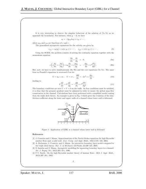
from the triple deck theory. An example is given in Fig. 1 which gives the evolution <strong>of</strong> the skinfriction<br />
coefficient along the lower and upper walls <strong>of</strong> a channel whose lower wall is deformed.<br />
References<br />
Cf<br />
upper<br />
wall<br />
0,0<br />
2 Re<br />
lower<br />
wall<br />
1.2<br />
1.0<br />
0.8<br />
0.6<br />
0.4<br />
0.2<br />
R =10 3<br />
x/L<br />
-5 -4 -3 -2 -1 0 1 2 3 4 5<br />
Figure 1: Application <strong>of</strong> GIBL in a channel whose lower wall is deformed<br />
[1] J. Cousteix and J. Mauss. Approximations <strong>of</strong> the Navier-Stokes equations for high Reynolds<br />
number flows past a solid wall. Jour. Comp. and Appl. Math., 166(1):101–122, 2004.<br />
[2] A. Dechaume, J. Cousteix, and J. Mauss. An interactive bo<strong>und</strong>ary layer model compared to<br />
the triple deck theory. Eur. J. <strong>of</strong> Mechanics B/Fluids, 24:439–447, 2005.<br />
[3] S. Saintlos and J. Mauss. Asymptotic modelling for separating bo<strong>und</strong>ary layers in a channel.<br />
Int. J. Engng. Sci., 34(2):201–211, 1996.<br />
[4] F.T. Smith. On the high Reynolds number theory <strong>of</strong> laminar flows. IMA J. Appl. Math.,<br />
28(3):207–281, 1982.<br />
Speaker: MAUSS, J. 117 <strong>BAIL</strong> <strong>2006</strong><br />
2<br />
✩<br />
✪


