Practical Implementation of PN Scrambler for PAPR Reduction
Practical Implementation of PN Scrambler for PAPR Reduction
Practical Implementation of PN Scrambler for PAPR Reduction

You also want an ePaper? Increase the reach of your titles
YUMPU automatically turns print PDFs into web optimized ePapers that Google loves.
PRACTICAL IMPLEMENTATION OF <strong>PN</strong> SCRAMBLER FOR <strong>PAPR</strong> REDUCTION IN OFDM<br />
SYSTEMS FOR RANGE EXTENSION AND LOWER POWER CONSUMPTION<br />
Christopher M<strong>of</strong>fatt<br />
Harris Corporation, Melbourne, FL, USA<br />
Christopher.M<strong>of</strong>fatt@Harris.com<br />
ABSTRACT<br />
Orthogonal Frequency Division Modulation (OFDM) is an<br />
efficient multi-carrier modulation scheme. It is used in<br />
many wireless communication systems due to its<br />
robustness towards fading channel behavior and a relative<br />
ease <strong>of</strong> implementation coming from computationally<br />
efficient Inverse Fast Fourier Trans<strong>for</strong>ms (IFFT).<br />
However, the OFDM wave<strong>for</strong>m has a very large Peak-to-<br />
Average Power Ratio (<strong>PAPR</strong>). There<strong>for</strong>e, to avoid clipping<br />
plus nonlinear distortion, the Power Amplifier (PA) needs<br />
to be backed <strong>of</strong>f significantly. This paper proposes a novel<br />
implementation and analysis <strong>of</strong> a Pseudorandom Noise<br />
(<strong>PN</strong>) scrambling technique allowing a significant<br />
reduction <strong>of</strong> the OFDM signal’s <strong>PAPR</strong>. The theoretical<br />
basis <strong>for</strong> the technique is presented, and a particular<br />
implementation <strong>of</strong> the technique <strong>for</strong> the IEEE 802.11a<br />
standard is discussed. Both simulations and measurements<br />
demonstrate significant benefits <strong>of</strong> the proposed technique<br />
in longer range wireless communications applications that<br />
use OFDM.<br />
1. INTRODUCTION<br />
Multi-carrier wave<strong>for</strong>ms <strong>for</strong> digital communications<br />
require a summation <strong>of</strong> multiple frequency-spaced singlecarriers<br />
prior to transmission through a Power Amplifier<br />
(PA). Orthogonal Frequency Division Multiplexing<br />
(OFDM) is a multi-carrier technique that utilizes hardware<br />
efficient IFFT to modulate each individual subcarrier with<br />
a Quadrature Amplitude Modulated (QAM) symbol and<br />
sum the subcarriers together to produce a single timedomain<br />
wave<strong>for</strong>m. The time-domain wave<strong>for</strong>m produced<br />
by addition <strong>of</strong> the independently modulated subcarriers has<br />
a very large Peak-to-Average Power Ratio (<strong>PAPR</strong>). As a<br />
result, the average power into the PA must be backed-<strong>of</strong>f<br />
to avoid clipping <strong>of</strong> the time-domain signal peaks.<br />
Clipping <strong>of</strong> the signal significantly increases the in-band<br />
noise (IBN) and the out-<strong>of</strong>-band noise (OBN) which<br />
adversely increases the bit-error rate (BER) and the<br />
adjacent channel interference (ACI), respectively. The<br />
large back<strong>of</strong>f necessary to avoid clipping and provide<br />
operation in the linear region <strong>of</strong> the PA requires higher<br />
power amplifiers at the transmitter and greatly increases<br />
system DC power consumption. For example, using 64<br />
sub-carriers, a 40 dBm power amplifier could require<br />
about 10 dB <strong>of</strong> back<strong>of</strong>f <strong>for</strong> a clipping probability <strong>of</strong><br />
978-1-4244-2677-5/08/$25.00 ©2008 IEEE<br />
1 <strong>of</strong> 7<br />
Ivica Kostanic, Ph.D.<br />
Florida Institute <strong>of</strong> Technology, Melbourne, FL, USA<br />
Kostanic@FIT.edu<br />
p=0.01%. There<strong>for</strong>e, instead <strong>of</strong> operating at 40 dBm (10<br />
Watts), the amplifier must be operated at 30 dBm (1 Watt)<br />
average power. Alternatively, in order to transmit at 40<br />
dBm, a 50 dBm (100 Watt) amplifier would be required.<br />
In practice however, large <strong>PAPR</strong> values occur infrequently,<br />
and the back<strong>of</strong>f is typically reduced down to a<br />
compression level that causes an acceptable amount <strong>of</strong><br />
distortion. Still, a large portion <strong>of</strong> the DC power<br />
consumed is wasted solely to maintain the linearity <strong>of</strong> the<br />
output PA stage. Thus, the use <strong>of</strong> <strong>PAPR</strong> reduction to<br />
allow less PA back<strong>of</strong>f is imperative to provide lower<br />
power requirements and extended battery operation.<br />
The outline <strong>of</strong> the paper is as follows. Section 2<br />
presents a brief overview <strong>of</strong> <strong>PAPR</strong> reduction techniques.<br />
Section 3 discusses the proposed <strong>PN</strong> scrambling-based<br />
<strong>PAPR</strong> reduction method. Section 4 describes a practical<br />
implementation <strong>of</strong> the <strong>PN</strong> <strong>Scrambler</strong> applied to an IEEE<br />
802.11a OFDM physical layer in an FPGA-based S<strong>of</strong>tware<br />
Defined Radio (SDR). Section 5 presents the example<br />
power savings applied to practical amplifiers. Finally,<br />
some conclusions are drawn in Section 6.<br />
2. <strong>PAPR</strong> REDUCTION METHODS<br />
The <strong>PAPR</strong> <strong>of</strong> a wave<strong>for</strong>m may be described [1] as<br />
2<br />
x(<br />
t)<br />
max<br />
<strong>PAPR</strong> = (1)<br />
Pavg<br />
where Pavg is the average power <strong>of</strong> the wave<strong>for</strong>m.<br />
In practical OFDM systems, the <strong>PAPR</strong> may be<br />
reduced using one or a combination <strong>of</strong> several techniques.<br />
The techniques may be divided into three major categories.<br />
The first category employs various methods <strong>of</strong> nonlinear<br />
signal distortion such as hard clipping [2], s<strong>of</strong>t clipping [3],<br />
companding [4], or pre-distortion [5]. Generally speaking,<br />
the nonlinear distortion techniques are simple to<br />
implement. However, many do not work well in cases<br />
where the OFDM sub-carriers are modulated with higherorder<br />
modulation schemes. In such scenarios, the<br />
Euclidian distance between the symbols is relatively small<br />
and the additional noise introduced by the <strong>PAPR</strong> reduction<br />
causes significant per<strong>for</strong>mance degradation.<br />
The second category <strong>for</strong> <strong>PAPR</strong> reduction employs<br />
various coding methods. The coding techniques [6] have<br />
an advantage <strong>of</strong> being distortionless and the <strong>PAPR</strong><br />
reduction is most commonly achieved by eliminating<br />
symbols having large <strong>PAPR</strong>. However, to obtain an<br />
appreciable level <strong>of</strong> <strong>PAPR</strong> reduction, high redundancy
codes need to be used and as a result, the overall efficiency<br />
<strong>of</strong> transmission becomes reduced.<br />
Finally, the third category is based on OFDM symbol<br />
scrambling and selection <strong>of</strong> the sequence that produces<br />
minimum <strong>PAPR</strong>. The pre-scrambling techniques [7-8]<br />
achieve good <strong>PAPR</strong> reduction but they require multiple<br />
FFT trans<strong>for</strong>ms and somewhat higher processing power.<br />
The method presented in this paper belongs to the third<br />
category <strong>of</strong> the <strong>PAPR</strong> reduction techniques. It uses<br />
conveniently chosen Pseudorandom Noise (<strong>PN</strong>) sequences<br />
applied to the input data bit stream. The method is very<br />
easy to realize in the s<strong>of</strong>tware or hardware environment<br />
which is very important if the <strong>PAPR</strong> needs to be<br />
implemented in Application Specific Integrated Circuits<br />
(ASIC). In such a scenario, the <strong>PN</strong>-<strong>Scrambler</strong> may be<br />
implemented by the addition <strong>of</strong> external FPGA and DSP<br />
hardware to the Commercial Off-The-Shelf (COTS)<br />
ASICs. As a result, one obtains cost efficient and reliable<br />
hardware solutions.<br />
3. OVERVIEW OF THE <strong>PN</strong>-SCRAMBLER<br />
TECHNIQUE FOR <strong>PAPR</strong> REDUCTION<br />
3.1. System overview<br />
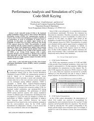
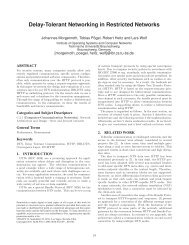
Block diagrams <strong>of</strong> the transmitter and receiver<br />
implementing the proposed <strong>PN</strong>-<strong>Scrambler</strong> are presented in<br />
Figs. 1 and 2, respectively.<br />
A/D Real<br />
A/D Imag<br />
Figure 1. <strong>PN</strong>-<strong>Scrambler</strong> Tx Block Diagram<br />
DC<br />
Offset<br />
DC<br />
Offset<br />
Subcarrier<br />
Demapper<br />
I / Q<br />
Imbalance<br />
I / Q<br />
Imbalance<br />
Channel<br />
Estimate<br />
Acquisition / Synchronization<br />
AGC<br />
Receive (Demodulation) Path<br />
Timing<br />
Detect<br />
Carrier<br />
Phase<br />
and<br />
Timing<br />
Drift<br />
Correction<br />
Coarse<br />
Freq<br />
S<strong>of</strong>t<br />
Bit<br />
Decisions<br />
Timing<br />
Fine<br />
Freq<br />
Deinterleaver<br />
and<br />
Convolutional<br />
decoder<br />
Sample<br />
Buffer<br />
Guard<br />
Interval<br />
Removal<br />
Descrambler<br />
FFT<br />
Data Bits<br />
Output<br />
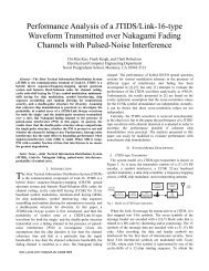
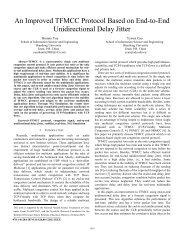
Figure 2. <strong>PN</strong>-<strong>Scrambler</strong> Rx Block Diagram<br />
As seen in Fig. 1, two additional elements are added to<br />
a typical OFDM transmitter. The first element is the<br />
<strong>PAPR</strong> scrambler, and the second one is the <strong>PAPR</strong><br />
threshold compare block. The <strong>PN</strong>-<strong>Scrambler</strong> utilizes a<br />
Maximal-Length Linear Feedback Shift Register (ML-<br />
LFSR) with log2(k) = l taps in order to produce k = 2 l -1<br />
uncorrelated unique sets <strong>of</strong> data from the same input<br />
sequence. The k unique sets <strong>of</strong> data are used to generate k<br />
independent identically distributed (i.i.d.) OFDM symbols.<br />
A block <strong>of</strong> Nb bits comprising one OFDM symbol is<br />
2 <strong>of</strong> 7<br />
scrambled and passed along <strong>for</strong> Forward Error Correction<br />
(FEC) coding, interleaving, modulation, symbol mapping<br />
and IFFT.<br />
In any given OFDM system, Nb is a function <strong>of</strong> the<br />
number <strong>of</strong> subcarriers, the modulation scheme applied to<br />
each subcarrier, and the coding rate. By examining each<br />
individual sample coming out <strong>of</strong> the IFFT, the <strong>PAPR</strong><br />
threshold comparator determines if the scrambler has<br />
achieved a desired <strong>PAPR</strong> on a symbol-by-symbol basis. If<br />
the <strong>PAPR</strong> <strong>of</strong> the symbol is below a desired threshold, then<br />
the data is passed along towards the RF stage <strong>of</strong> the<br />
transmitter. However, if the <strong>PAPR</strong> is still high, the data is<br />
scrambled with a different phase <strong>of</strong> the ML-LFSR’s <strong>PN</strong><br />
sequence. Since this technique operates on the input bit<br />
stream, it is essentially independent <strong>of</strong> the OFDM<br />
modulation and may be adapted to any particular scenario.<br />
The receiver presented in Fig. 2 is a typical OFDM<br />
receiver that needs to per<strong>for</strong>m the tasks <strong>of</strong> down<br />
conversion, channel estimation, and decoding. The only<br />
additional task required by the <strong>PN</strong>-<strong>Scrambler</strong> <strong>PAPR</strong><br />
reduction technique is descrambling <strong>of</strong> the data at the<br />
receiver output. To per<strong>for</strong>m descrambling, the receiver<br />
has to “know” the phase <strong>of</strong> the ML-LFSR used on the<br />
transmission side. This phase is embedded in the data<br />
stream. For example, the first l bits <strong>of</strong> the OFDM symbol<br />
may carry the in<strong>for</strong>mation on the ML-LFSR phase.<br />
3.2. Analytical Per<strong>for</strong>mance Characterization<br />
A practical implementation <strong>of</strong> the <strong>PN</strong>-<strong>Scrambler</strong><br />
<strong>PAPR</strong> reduction technique requires selection <strong>of</strong> several<br />
parameters. These parameters are defined as follows.<br />
1. Number <strong>of</strong> scrambling sequences (k) - defined as the<br />
number <strong>of</strong> <strong>PN</strong> sequences produced by the ML-<br />
LFSR. Each sequence is Nb bits long.<br />
2. <strong>PAPR</strong> threshold (L) – defined as the maximum<br />
<strong>PAPR</strong> <strong>for</strong> the OFDM symbol. This value is used by<br />
the <strong>PAPR</strong> threshold comparator block in order to<br />
discard OFDM symbols with <strong>PAPR</strong> greater than L.<br />
3. IFFT size / number <strong>of</strong> sub-carriers (N) – defined as<br />
the number <strong>of</strong> the non-zero orthogonal subcarriers<br />
per OFDM symbol.<br />
4. Average latency ( k ) – defined as the average<br />
number <strong>of</strong> scrambling attempts per OFDM symbol<br />
in order to pass the threshold level L.<br />
5. Probability <strong>of</strong> clipping (p) – probability that the<br />
<strong>PAPR</strong> exceeds the threshold level L after k<br />
scrambling attempts.<br />
6. <strong>PN</strong> scrambler overhead ( v ) – defined as the ratio <strong>of</strong><br />
the number <strong>of</strong> bits required to represent the phase <strong>of</strong><br />
the ML-LFSR to the number <strong>of</strong> bits per OFDM<br />
symbol Nb.<br />
In any actual design, the above parameters allow different<br />
trade<strong>of</strong>fs. The subsequent section highlights some <strong>of</strong> these<br />
design trades.
3.3. <strong>PAPR</strong> per OFDM Sample after Application <strong>of</strong> k-<br />
<strong>PN</strong> Scrambling Sequences<br />
The goal <strong>of</strong> the analysis presented in this section is to<br />
find the analytical <strong>PAPR</strong> probability distribution <strong>of</strong> the<br />
<strong>PN</strong>-scrambled OFDM signal on a sample-by-sample basis.<br />
This allows the <strong>PAPR</strong> to be compared with other sampled<br />
time-domain signals and techniques. Define the complex<br />
baseband signal as<br />
S = X + jY , where j = −1<br />
(2)<br />
From the central limit theorem, the OFDM signal will have<br />
a Gaussian probability density function (PDF) <strong>for</strong> both the<br />
real X and imaginary Y time-domain signals due to the<br />
addition <strong>of</strong> multiple complex exponentials with random<br />
amplitude A and phase θ.<br />
N −1<br />
N −1<br />
⎛ 2π<br />
nk ⎞<br />
⎛ 2πnk<br />
⎞ ⎛ 2πnk<br />
⎞ (3)<br />
∑ Ak ⋅ exp⎜<br />
j ⋅ + jθ<br />
k ⎟ = ∑ Ak<br />
⋅ cos⎜<br />
+ θ k ⎟ + j ⋅ Ak<br />
⋅ sin⎜<br />
+ θ k ⎟<br />
n=<br />
0 ⎝ N ⎠ n=<br />
0 ⎝ N ⎠ ⎝ N ⎠<br />
Then, the magnitude R, is<br />
R +<br />
The magnitude <strong>of</strong> the complex baseband signal can be<br />
approximated as Rayleigh distributed, since the real and<br />
imaginary components X and Y are independent Gaussian<br />
random variables with zero mean and equal variances σ 2 .<br />
Interestingly, the original derivation <strong>of</strong> this density<br />
function by Lord Rayleigh in 1880 was applied to the<br />
similar application <strong>of</strong> finding the envelope <strong>of</strong> the sum <strong>of</strong><br />
many sine waves <strong>of</strong> different frequencies. The Rayleigh<br />
PDF is given by [9] as<br />
2<br />
⎧ r ⎛ r ⎞<br />
⎪ exp<br />
≥<br />
⎨ ⎜<br />
⎜−<br />
⎟ r 0<br />
f ( r)<br />
= 2<br />
2<br />
(5)<br />
R σ ⎝ 2 ⋅σ<br />
⎠<br />
⎪<br />
⎩ 0 r < 0<br />
The PDF <strong>of</strong> the power signal <strong>of</strong> a complex Gaussian signal<br />
is derived using a trans<strong>for</strong>mation <strong>of</strong> random variables,<br />
where it is desired to find the power random variable<br />
2<br />
W = R<br />
(6)<br />
Using a trans<strong>for</strong>mation <strong>of</strong> random variables<br />
dr<br />
fW ( w)<br />
= f R ( r)<br />
⋅<br />
(7)<br />
dw<br />
The complex 1 power PDF can be written as<br />
⎧⎛<br />
1 ⎞ ⎛ w ⎞<br />
⎪⎜<br />
⎟ ⋅ exp⎜<br />
− ⎟ w ≥ 0<br />
f ( w)<br />
=<br />
2<br />
2<br />
⎨<br />
(8)<br />
W ⎝ 2 ⋅σ<br />
⎠ ⎝ 2 ⋅σ<br />
⎠<br />
⎪<br />
⎩ 0<br />
w < 0<br />
The complex power CDF <strong>of</strong> a complex signal with<br />
Gaussian real and imaginary components is given by<br />
w<br />
⎛ 1 ⎞ ⎛ u ⎞<br />
Pr( W ≤ w)<br />
= FW<br />
( w)<br />
= ∫ ⎜ ⎟ ⋅exp⎜<br />
− ⎟du (9)<br />
2<br />
2<br />
0 ⎝ 2⋅σ<br />
⎠ ⎝ 2⋅σ<br />
⎠<br />
Since this is an indeterminate integral, it cannot be<br />
represented in closed-<strong>for</strong>m solution. However, it is still<br />
2 2<br />
= X Y<br />
(4)<br />
1 The term “complex” power refers to the OFDM complex baseband<br />
signal in order to avoid confusion from the power PDF <strong>of</strong> a real variable.<br />
3 <strong>of</strong> 7<br />
possible to find the complex power CDF 2 by taking<br />
advantage <strong>of</strong> the Rayleigh CDF.<br />
2<br />
W = R<br />
2 2<br />
= X + Y<br />
(10)<br />
The complex power CDF is given by,<br />
FW ( w)<br />
= Pr( R ≤ + w)<br />
− Pr( R ≤ − w)<br />
(11)<br />
Then, the probability that the power is less than or equal to<br />
some value w is simply the probability that the magnitude<br />
is between the values <strong>of</strong> + w and − w . The CDF <strong>for</strong> the<br />
magnitude R is the Rayleigh CDF<br />
2<br />
⎧ ⎛ r ⎞<br />
⎪1<br />
− exp<br />
⎨ ⎜<br />
⎜−<br />
⎟<br />
Pr( R ≤ r)<br />
= F ( ) =<br />
2<br />
R r<br />
⎝ 2 ⋅σ<br />
⎠<br />
⎪<br />
⎩ 0<br />
r ≥ 0 (12)<br />
r < 0<br />
Substituting equation (12) into equation (11) and using the<br />
fact that FR ( − w)<br />
= 0 since FR ( r)<br />
= 0 when r < 0<br />
⎧ ⎛ w ⎞<br />
⎪1<br />
− exp⎜<br />
−<br />
Pr( W ≤ w)<br />
= F ( ) =<br />
2 ⎟<br />
W w ⎨ ⎝ 2 ⋅σ<br />
⎠<br />
⎪<br />
⎩ 0<br />
w ≥ 0<br />
w < 0<br />
(13)<br />
The peak power per OFDM symbol is measured as the<br />
largest power sample out <strong>of</strong> the N corresponding complex<br />
samples. It is desired to find the probability that the peak<br />
power <strong>of</strong> at least one out <strong>of</strong> N samples exceeds a<br />
predetermined peak power threshold level L. We start by<br />
defining event A as the event that the complex timedomain<br />
sample’s power w exceeds threshold L. We want<br />
to find the probability that event A occurs at least m=1<br />
time out <strong>of</strong> the N OFDM symbol samples. Since each<br />
time-domain sample is i.i.d., the Bernoulli trials can be<br />
useful here<br />
Pr{A occurs m times} =<br />
⎛ N ⎞ m N −m<br />
g N ( m)<br />
= ⎜ ⎟ ⋅ p q (14)<br />
⎝ m ⎠<br />
⎛ N ⎞<br />
N!<br />
⎜ ⎟=<br />
N Cm<br />
=<br />
(15)<br />
⎝ m ⎠ m!<br />
( N − m)!<br />
Using the Binomial distribution, we can write<br />
Pr{A occurs at least m times in N samples}=<br />
N<br />
N ⎛ N ⎞ i N −i<br />
∑ g N ( i)<br />
= ∑⎜<br />
⎟ ⋅ p q<br />
(16)<br />
i=<br />
m<br />
i=<br />
m ⎝ i ⎠<br />
where p is the probability that a single complex timedomain<br />
sample exceeds L, defined as<br />
2 { x + jy > L}<br />
= 1−<br />
F ( L)<br />
p = Pr<br />
(17)<br />
w<br />
q W<br />
= 1− p = F ( L)<br />
(18)<br />
2 The probability distribution function, or cumulative distribution<br />
function (CDF), is defined by [10] to be the probability <strong>of</strong> the event that<br />
the observed random variable W is less than or equal to the allowed<br />
value w. In this case, W is the random variable and the value w will<br />
later represent a power threshold level and will be substituted with the<br />
variable L.
The probability that the power W > L occurs at least m=1<br />
time out <strong>of</strong> N samples is<br />
Pr{A occurs at least 1 time in N samples} =<br />
N ⎛ N ⎞ i N −i<br />
∑= ⎜ ⎟ ⋅ p q<br />
i 1 ⎝ i ⎠<br />
(19)<br />
In order to simplify the equation, note that the probability<br />
W > L occurs at least m=1 time out <strong>of</strong> N samples is the<br />
same as the complementary probability that exactly no<br />
samples (m=0) have W > L, which can be written as<br />
1-Pr{A occurs exactly 0 times out <strong>of</strong> N samples} =<br />
⎛ N ⎞ N<br />
N<br />
N<br />
1−<br />
g N ( 0)<br />
= 1−<br />
⎜ ⎟ ⋅ p q = 1−<br />
q = 1−<br />
( 1−<br />
p)<br />
= 1−<br />
F<br />
⎝ 0 ⎠<br />
0 N<br />
W ( L)<br />
(20)<br />
Thus, we now define the CCDF <strong>of</strong> the peak power per<br />
OFDM symbol as the probability that the peak power <strong>of</strong><br />
one sample out <strong>of</strong> N samples exceeds threshold L<br />
N<br />
⎛ ⎛ L ⎞⎞<br />
Fsym = Pr{<br />
PeakPowerOFDM<br />
_ Symbol > L}<br />
= 1−<br />
⎜1<br />
− exp⎜<br />
− ⎟⎟<br />
2<br />
⎝ ⎝ 2 ⋅σ<br />
⎠⎠<br />
(21)<br />
Using the <strong>PN</strong> scrambler to generate k OFDM symbols and<br />
then selecting the OFDM symbol with the lowest <strong>PAPR</strong><br />
<strong>for</strong> transmission reduces the peak power probability to p k .<br />
For example, if an OFDM symbol has the probability <strong>of</strong><br />
p=0.1 <strong>of</strong> exceeding threshold L, then the probability <strong>of</strong> k=2<br />
OFDM symbols exceeding threshold L is (0.1) 2 =0.01.<br />
This is true because <strong>of</strong> the statistical independence <strong>of</strong> the<br />
peak power between OFDM symbols generated by the <strong>PN</strong>-<br />
<strong>Scrambler</strong> (i.e. uncorrelated data sets). That is, if the<br />
probability <strong>of</strong> event S1 does not depend upon the outcome<br />
<strong>of</strong> S2 and visa versa, such events are said to be statistically<br />
independent and<br />
Pr(S , S )<br />
=<br />
1<br />
2<br />
2<br />
= Pr(S1)<br />
⋅ Pr(S2)<br />
= p ⋅ p p (22)<br />
For k statistically independent events, this becomes<br />
Pr(S , S ,..., S )<br />
=<br />
1<br />
2<br />
k<br />
k<br />
= Pr(S1)<br />
⋅Pr(S2<br />
) ⋅⋅⋅<br />
Pr(Sk<br />
) = p⋅<br />
p⋅<br />
⋅⋅<br />
p p (23)<br />
For k scrambling sequences, the new <strong>PAPR</strong> CCDF per<br />
OFDM symbol can now be <strong>for</strong>mally written as<br />
Pr<br />
{ <strong>PAPR</strong> k > L}<br />
OFDM _ Symbol sequences<br />
N<br />
⎛<br />
⎞<br />
⎜ ⎛ ⎛ L ⎞⎞<br />
= 1−<br />
⎜1−<br />
exp⎜<br />
− ⎟⎟<br />
⎟<br />
⎜<br />
2<br />
2 ⎟<br />
⎝ ⎝ ⎝ ⋅σ<br />
⎠⎠<br />
⎠<br />
k<br />
2 1<br />
σ =<br />
2<br />
(24)<br />
Substituting equation (13) into (21) yields<br />
F = 1 − F<br />
N<br />
(25)<br />
sym<br />
W<br />
4 <strong>of</strong> 7<br />
Rearranging, the sample-based power distribution is<br />
related to the OFDM symbol-based peak power<br />
distribution by<br />
( ) N<br />
1<br />
FW<br />
= 1− F<br />
(26)<br />
sym<br />
Next, we define the new <strong>PAPR</strong> distribution Fsym ˆ as the<br />
OFDM symbol-based peak-power distribution after k<br />
scrambling sequences<br />
k<br />
N k<br />
F ˆ<br />
sym = Fsym<br />
= ( 1 − FW<br />
)<br />
(27)<br />
Finally, in order to determine FW ˆ , which is the new <strong>PAPR</strong><br />
reduced sample-based power distribution after application<br />
<strong>of</strong> k scrambling sequences, we simply substitute Fsym ˆ into<br />
equation (26) relating the sample-based power distribution<br />
to the OFDM symbol-based peak power distribution,<br />
Fˆ<br />
W<br />
=<br />
1<br />
N<br />
N k<br />
( 1 − Fˆ<br />
) = ( 1 − ( 1 − F ) )<br />
sym<br />
W<br />
1<br />
N<br />
1<br />
N<br />
k N<br />
⎛<br />
⎞<br />
⎜ ⎛<br />
L ⎞<br />
1 ⎜ ⎛ ⎛ ⎞⎞<br />
⎟<br />
= ⎜ − 1 − ⎜1<br />
− exp⎜<br />
− ⎟ ⎟<br />
2 ⎟<br />
2<br />
⎟<br />
⎜ ⎜<br />
⎟ ⎟<br />
⎝ ⎝ ⎝ ⎝ ⋅σ<br />
⎠⎠<br />
⎠ ⎠<br />
(28)<br />
In the above equation, FW ˆ is the CDF <strong>of</strong> the <strong>PAPR</strong><br />
reduced sample-based distribution using k-scrambling<br />
sequences, which is the probability that each individual<br />
sample’s peak power is less than or equal to threshold<br />
level L using an IFFT size <strong>of</strong> N. It is more useful to<br />
evaluate the probability that each individual sample’s peak<br />
power is greater than threshold level L, which is the<br />
complementary CDF, CCDF=1-CDF.<br />
1<br />
k<br />
N<br />
N<br />
⎛<br />
⎞<br />
⎜ ⎛<br />
L ⎞<br />
CCDF(<br />
L,<br />
N,<br />
k)<br />
1 1 ⎜ ⎛ ⎛ ⎞⎞<br />
⎟<br />
= − ⎜ − 1−<br />
⎜1−<br />
exp⎜<br />
− ⎟ ⎟<br />
2 ⎟<br />
2<br />
⎟<br />
⎜ ⎜<br />
⎟ ⎟<br />
⎝ ⎝ ⎝ ⎝ ⋅σ<br />
⎠⎠<br />
⎠ ⎠<br />
(29)<br />
After normalization <strong>of</strong> the complex time-domain signal’s<br />
average power<br />
<strong>PAPR</strong><br />
CCDF<br />
1<br />
N k N<br />
= 1−<br />
⎜<br />
⎛1− ( 1−<br />
( 1−<br />
exp(<br />
− L)<br />
) ) ⎞ (30)<br />
( L,<br />
N,<br />
k)<br />
⎟<br />
⎝<br />
⎠<br />
It is important to note that due to the equivalence<br />
theorem, the analysis and linear signal processing <strong>of</strong><br />
baseband wave<strong>for</strong>m presented herein will be identical to<br />
the analysis <strong>of</strong> the bandpass wave<strong>for</strong>m with the exception<br />
<strong>of</strong> oversampling error. A rigorous discussion <strong>of</strong> the <strong>PAPR</strong><br />
measurement error due to Nyquist sampling versus<br />
continuous sampling can be found in [10]. Because most<br />
applications are typically concerned with the probability<br />
that a signal’s power exceeds a certain level L, instead <strong>of</strong><br />
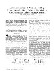
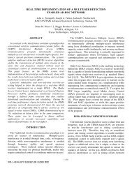
using the CDF, the CCDF is typically plotted and is shown<br />
in Fig. 3 <strong>for</strong> FFT sizes N=64, N=128, N=256 and number<br />
<strong>of</strong> scrambling sequences k=1 (i.e. no <strong>PAPR</strong> reduction),<br />
k=8, and k=256. The plot shows both the theoretical<br />
curves obtained using equation (30) and the empirical<br />
curves obtained through computer simulations.
Probability <strong>of</strong> <strong>PAPR</strong> > x dB<br />
10 -1<br />
10 -2<br />
10 -3<br />
10 -4<br />
10 -5<br />
CCDF Curve<br />
Analytical <strong>PAPR</strong> CCDF<br />
Empirical Prob k: 1 FFT SIZE: 64<br />
Derived Prob k: 1 FFT SIZE: 64<br />
Empirical Prob k: 16 FFT SIZE: 64<br />
Derived Prob k: 16 FFT SIZE: 64<br />
Empirical Prob k: 256 FFT SIZE: 64<br />
Derived Prob k: 256 FFT SIZE: 64<br />
Empirical Prob k: 1 FFT SIZE: 128<br />
Derived Prob k: 1 FFT SIZE: 128<br />
Empirical Prob k: 16 FFT SIZE: 128<br />
Derived Prob k: 16 FFT SIZE: 128<br />
Empirical Prob k: 256 FFT SIZE: 128<br />
Derived Prob k: 256 FFT SIZE: 128<br />
Empirical Prob k: 1 FFT SIZE: 256<br />
Derived Prob k: 1 FFT SIZE: 256<br />
Empirical Prob k: 16 FFT SIZE: 256<br />
Derived Prob k: 16 FFT SIZE: 256<br />
Empirical Prob k: 256 FFT SIZE: 256<br />
Derived Prob k: 256 FFT SIZE: 256<br />
10<br />
0 2 4 6 8 10 12<br />
-6<br />
x dB<br />
Figure 3. <strong>PAPR</strong> probability distribution per sample using<br />
k-<strong>PN</strong> scrambling sequences<br />
Figure 3 shows that the <strong>PAPR</strong> probability given in<br />
equation (30) matches the simulated data very closely.<br />
The figure shows a significant reduction in <strong>PAPR</strong> due to<br />
application <strong>of</strong> the k-<strong>PN</strong> scrambling sequences. For<br />
example, <strong>for</strong> N=64 subcarriers, the figure indicates the<br />
probability that the <strong>PAPR</strong> exceeds L=4.5 dB reduces from<br />
p=6.0% at k=1 down to p=0.01% at k=256. In order to<br />
ensure that the <strong>PAPR</strong> is less than L at p=0.01% <strong>of</strong> the time<br />
<strong>for</strong> conventional OFDM (i.e. k=1), the equivalent <strong>PAPR</strong><br />
threshold is L=9.6dB. If the OFDM signal is input into an<br />
ideal amplifier that clips the signal when it is larger than<br />
the saturation point and it is desired to not clip the signal<br />
more than p=0.01% <strong>of</strong> the time, then application <strong>of</strong> the<br />
k=256 scrambling sequences requires 9.6-4.5=5.1 dB less<br />
back<strong>of</strong>f. Often a larger amount <strong>of</strong> in-band noise and out<strong>of</strong>-band<br />
noise can be tolerated and there<strong>for</strong>e a higher<br />
clipping probability is acceptable. There<strong>for</strong>e, in a typical<br />
system, less than 5.1 dB per<strong>for</strong>mance is gained due to<br />
application <strong>of</strong> the k=256 scrambling sequences.<br />
Probability <strong>of</strong> <strong>PAPR</strong> > L dB<br />
10 0<br />
10 -1<br />
10 -2<br />
10 -3<br />
10 -4<br />
10 -5<br />
CCDF Curve Vs. Threshold L and k-<strong>PN</strong> Scrambling Sequences<br />
k=256<br />
Increasing k Scrambling Sequences<br />
10<br />
0 2 4 6 8 10 12<br />
-6<br />
L dB<br />
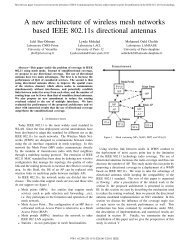
Figure 4. CCDF Curve Probability <strong>PAPR</strong>>L, multiple k-<br />
<strong>PN</strong> scrambling sequences overlaid (k=1:1:256)<br />
k=1<br />
5 <strong>of</strong> 7<br />
The CCDF curves in Fig. 4 show rapid <strong>PAPR</strong> reduction<br />
during the first few k scrambling sequences. After about<br />
k=8, the <strong>PAPR</strong> reduction begins to approach diminishing<br />
returns. For example, at k=128 and k=129 the probability<br />
p=Pr{<strong>PAPR</strong>>L}=0.01% occurs at threshold L=4.7786 dB<br />
and L=4.7753 dB, respectively. This results in a small<br />
improvement <strong>of</strong> ΔL=0.0033 dB, which is insignificant<br />
compared to ΔL=1.4 dB from k=1 to k=2.<br />
3.4. <strong>Practical</strong> Example<br />
As a practical example, consider the following design<br />
problem. An OFDM transmitter with N=64 subcarriers<br />
must be designed. As part <strong>of</strong> the design problem, the<br />
transmitter must achieve a low latency and there<strong>for</strong>e use<br />
no more than k=256 scrambling sequences per OFDM<br />
symbol. Each OFDM symbol is compared to a threshold<br />
level L. If the OFDM symbol’s peak power exceeds the<br />
threshold level L, it is re-generated using the <strong>PN</strong>-<br />
<strong>Scrambler</strong> until the symbol’s peak power is smaller than L.<br />
As soon as the OFDM symbol has a peak power less than<br />
L, it is stored in a packet buffer where it waits to be<br />
transmitted. Once the desired number <strong>of</strong> “symbols per<br />
packet” is stored in the packet buffer, the packet is<br />
immediately transmitted out the digital-to-analog converter<br />
(DAC). Since the <strong>PN</strong>-<strong>Scrambler</strong> in this example is only<br />
l=8-bits, the ML-LFSR can only generate k=2 8 -1=255<br />
possible unique OFDM symbols that represent the same<br />
data. Since the transmitter already has a data whitener, an<br />
additional bypass mode is added to provide a total <strong>of</strong><br />
k=255+1=256 possible unique OFDM symbols that<br />
represent the same data. If any <strong>of</strong> the symbols exceed the<br />
k=256 scrambling sequences, the symbol with the lowest<br />
<strong>PAPR</strong> out <strong>of</strong> the 256 will be selected <strong>for</strong> transmission.<br />
However, this means that one or more <strong>of</strong> the symbols in<br />
the packet buffer did not pass the threshold level L and<br />
may be clipped by the DAC or PA. There<strong>for</strong>e, in order to<br />
ensure that this does not happen <strong>of</strong>ten, we desire a very<br />
low probability <strong>of</strong> 1 in 10,000 OFDM symbols requiring<br />
more than k=256 <strong>PN</strong>-Sequences, or equivalently, p=10 -4 .<br />
The problem is to determine the value <strong>of</strong> the threshold<br />
level L and the average number <strong>of</strong> k-<strong>PN</strong> scrambling<br />
sequences that will be generated as a result <strong>of</strong> the<br />
corresponding threshold level setting.<br />
We start by noting the latency requirement and let<br />
m=256, the number <strong>of</strong> sequences not to exceed. For this<br />
example,<br />
−4<br />
p = Pr( k > m)<br />
= Pr( k > 256)<br />
= 10 (31)<br />
Both L and N are predetermined constants in the<br />
transmitter and receiver and k is the random variable,<br />
f<br />
W , k<br />
( L,<br />
N,<br />
k)<br />
dF<br />
=<br />
W , k<br />
( L,<br />
N,<br />
k)<br />
dk<br />
k<br />
⎛<br />
N ⎞<br />
⎜ ⎛<br />
L ⎞ ⎟<br />
d ⎜ ⎛ ⎛ ⎞⎞<br />
⎟<br />
⎜1−<br />
1−<br />
⎜1−<br />
exp⎜−<br />
⎟ 2 ⎟ ⎟<br />
⎜ ⎜<br />
⎟ ⎟<br />
⎝ ⎝ ⎝ ⎝ 2⋅σ<br />
⎠⎠<br />
⎠<br />
=<br />
⎠<br />
dk<br />
(32)
After evaluating the derivative with respect to k, the joint<br />
PDF is given as<br />
f<br />
W , k<br />
( L,<br />
N,<br />
k)<br />
N<br />
N<br />
⎛<br />
L ⎞ ⎛<br />
L ⎞<br />
⎜ ⎛ ⎛ ⎞⎞<br />
⎜ ⎛ ⎛ ⎞⎞<br />
− ln 1−<br />
⎜1−<br />
exp⎜−<br />
⎟⎟<br />
⎟ ⋅ 1−<br />
⎜1−<br />
exp⎜−<br />
⎟⎟<br />
⎟<br />
2<br />
⎜<br />
⎟ ⎜<br />
⎟<br />
⎝ ⎝ ⎝ 2 ⋅σ<br />
⎠⎠<br />
⎠ ⎝ ⎝ ⎝ 2 ⋅σ<br />
⎠⎠<br />
⎠<br />
= 2<br />
The probability in (31) can now be found by integrating<br />
the joint PDF over the range <strong>of</strong> k,<br />
( L,<br />
N,<br />
k)<br />
dk = p<br />
k<br />
(33)<br />
k m<br />
k > = − ∫ f<br />
=<br />
Pr( 256)<br />
1<br />
(34)<br />
W , k<br />
k =0<br />
Equation 34 can be solved <strong>for</strong> L to obtain<br />
⎛<br />
⎜ ⎛<br />
L = − ln⎜1<br />
− ⎜<br />
1−<br />
p<br />
⎜ ⎝<br />
⎝<br />
1<br />
1 N<br />
m<br />
⎞<br />
⎟<br />
⎠<br />
⎞<br />
⎟<br />
⎟<br />
⎟<br />
⎠<br />
(35)<br />
Equation (35) can be used to find the required <strong>PAPR</strong><br />
threshold level L <strong>for</strong> any FFT size N. The value m in (35)<br />
is the desired number <strong>of</strong> k-<strong>PN</strong> scrambling sequences not to<br />
exceed. The value p in (35) specifies the probability that a<br />
given OFDM symbol will not require more than m<br />
scrambling sequences in order to pass the objective <strong>PAPR</strong><br />
threshold level setting L. Evaluating (35) using p=10 -4 ,<br />
m=256, and N=64 yields the required <strong>PAPR</strong> threshold<br />
level setting L=2.98 or 4.74 dB.<br />
In order to find the average number <strong>of</strong> scrambling<br />
sequences, it is convenient to make use <strong>of</strong> the definition <strong>of</strong><br />
the expected value <strong>of</strong> a random variable,<br />
∞<br />
∫<br />
−∞<br />
X = E[<br />
X ] = x ⋅ f ( x)<br />
dx<br />
(36)<br />
The average number <strong>of</strong> scrambling sequences k becomes<br />
= ∞<br />
∫<br />
=<br />
⎟ ⎟⎟<br />
k ⎛<br />
N<br />
N<br />
k ⎞<br />
⎜ ⎛<br />
⎞ ⎛<br />
⎞<br />
⎜ ⎛ ⎛ L ⎞⎞<br />
⎟ ⎜ ⎛ ⎛ L ⎞⎞<br />
(37)<br />
k = k ⋅<br />
⎟<br />
⎜−<br />
ln 1−<br />
⎜1−<br />
exp⎜−<br />
⎟⎟<br />
⋅ 1−<br />
⎜1−<br />
exp⎜−<br />
⎟⎟<br />
dk<br />
2<br />
2<br />
⎜ ⎜<br />
⎟ ⎜<br />
⎟<br />
⎝ ⎝ ⎝ ⎝ 2⋅σ<br />
⎠⎠<br />
⎠ ⎝ ⎝ ⎝ 2⋅σ<br />
k 0<br />
⎠⎠<br />
⎠ ⎠<br />
After simplification,<br />
−1<br />
(38)<br />
k =<br />
N<br />
⎛<br />
⎞<br />
⎜ ⎛ ⎛ L ⎞⎞<br />
ln 1−<br />
⎜1−<br />
exp⎜<br />
− ⎟⎟<br />
⎟<br />
⎜<br />
2 ⎟<br />
⎝ ⎝ ⎝ 2⋅σ<br />
⎠⎠<br />
⎠<br />
For this example, the average number <strong>of</strong> <strong>PN</strong> scrambling<br />
sequences that will occur at this <strong>PAPR</strong> threshold level<br />
setting is<br />
( ( ( ) ) ) 27.8<br />
1<br />
64<br />
ln 1 1 exp 2.<br />
98<br />
=<br />
−<br />
k =<br />
(39)<br />
− − −<br />
Using 64-QAM modulation per subcarrier, the<br />
overhead v <strong>for</strong> this example is<br />
log 2 ( m)<br />
log ( 256)<br />
(40)<br />
2<br />
v =<br />
= = 0.<br />
028<br />
N ⋅ N ⋅ C 3<br />
bps 64 ⋅ 6 ⋅<br />
4<br />
where m is the number <strong>of</strong> sequences not to exceed, N is the<br />
number <strong>of</strong> subcarriers, Nbps is the number <strong>of</strong> bits per<br />
subcarrier based on the constellation size, and C is the<br />
FEC code rate.<br />
6 <strong>of</strong> 7<br />
In summary, in order to ensure that the OFDM<br />
transmitter does not exceed k=256 <strong>PN</strong> scrambling<br />
sequences with a probability <strong>of</strong> p=10 -4 , the peak power<br />
threshold level must be set to L=4.74 dB which will<br />
require approximately k=28 <strong>PN</strong> scrambling sequences on<br />
average. In other words, the system will have a <strong>PAPR</strong> less<br />
than or equal to 4.74 dB with a 99.9900% probability.<br />
Without the symbol scrambling (i.e. k=1), the <strong>PAPR</strong> is<br />
11.3 dB at p=10 -4 . Using the system parameters derived in<br />
this example, this technique results in an improvement <strong>of</strong><br />
6.5 dB with an insignificant overhead <strong>of</strong> 2.8%.<br />
4. PRACTICAL IMPLEMENTATION<br />
The <strong>PN</strong>-<strong>Scrambler</strong> was implemented as a <strong>PAPR</strong><br />
reduction technique <strong>for</strong> an IEEE 802.11a OFDM modem.<br />
Without application <strong>of</strong> the <strong>PAPR</strong> reduction, the CCDF<br />
curve <strong>for</strong> the IEEE 802.11a OFDM modem closely follows<br />
the k = 1 curve <strong>of</strong> Fig. 3, indicating that the IEEE 802.11a<br />
wave<strong>for</strong>m has a large <strong>PAPR</strong>.<br />
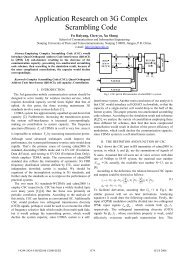
<strong>PAPR</strong> <strong>Reduction</strong> ON<br />
<strong>PAPR</strong> <strong>Reduction</strong> ON<br />
Back<strong>of</strong>f = 8 dB<br />
Back<strong>of</strong>f = 8 dB<br />
EVM = -40.34 dB<br />
EVM = -40.34 dB<br />
<strong>PAPR</strong> <strong>Reduction</strong> ON<br />
<strong>PAPR</strong> <strong>Reduction</strong> ON<br />
Back<strong>of</strong>f = 5 dB<br />
Back<strong>of</strong>f = 5 dB<br />
EVM = -33.44 dB<br />
EVM = -33.44 dB<br />
<strong>PAPR</strong> <strong>Reduction</strong> OFF<br />
<strong>PAPR</strong> <strong>Reduction</strong> OFF<br />
Back<strong>of</strong>f = 8 dB<br />
Back<strong>of</strong>f = 8 dB<br />
EVM = -34.35 dB<br />
EVM = -34.35 dB<br />
<strong>PAPR</strong> <strong>Reduction</strong> OFF<br />
<strong>PAPR</strong> <strong>Reduction</strong> OFF<br />
Back<strong>of</strong>f = 5 dB<br />
Back<strong>of</strong>f = 5 dB<br />
EVM = -25.40 dB<br />
EVM = -25.40 dB<br />
Figure 5. VSA EVM plots with and without<br />
<strong>PAPR</strong> reduction<br />
The OFDM signal from the output <strong>of</strong> the I/Q<br />
modulator was sent through a 10-Watt Stealth Microwave<br />
Class-A Power Amplifier (SM0825-40) into an Agilent<br />
Vector Signal Analyzer 89641A (VSA). The VSA<br />
demodulated the OFDM signal and the resulting<br />
constellations are shown in Fig. 5. The results show<br />
significant reduction in the Error Vector Magnitude<br />
(EVM) with <strong>PAPR</strong> reduction “on” versus with <strong>PAPR</strong><br />
reduction “<strong>of</strong>f.” Furthermore, the results show that at 8 dB<br />
back<strong>of</strong>f from the power amplifier’s one dB compression<br />
point (P1dB) with <strong>PAPR</strong> reduction turned-<strong>of</strong>f produces<br />
approximately the same EVM as 5 dB back<strong>of</strong>f when the<br />
<strong>PAPR</strong> reduction is turned-on. This 3 dB reduction in<br />
back<strong>of</strong>f provides twice the RF output transmit power, or<br />
equivalently, allows a 10-Watt amplifier to be used instead<br />
<strong>of</strong> a 20-Watt amplifier.
5. POWER SAVINGS<br />
The power consumption <strong>of</strong> communication systems is<br />
typically determined by the power requirements <strong>of</strong> the<br />
final power amplifier. From the CCDF curves given in Fig.<br />
3, it can be observed that the <strong>PN</strong>-<strong>Scrambler</strong> technique<br />
provides considerable reduction <strong>of</strong> the <strong>PAPR</strong>. As a result,<br />
the average power <strong>of</strong> the PA may be set closer to its<br />
maximum power level. For a Class-A Linear PA, a 3 dB<br />
lower P1dB-point typically corresponds to a reduction <strong>of</strong><br />
DC power consumption by half (see Table 1 <strong>for</strong> examples).<br />
Table 1- Class-A Power Amplifiers<br />
(Courtesy <strong>of</strong> Stealth Microwave)<br />
Class-A Linear Frequency RF Output Power RF Output DC Voltage Current Power<br />
Power Amplifier Range (MHz) P1dB (dBm) Power (Watts) (V) (Amps) (Watts)<br />
SM1720-37H 1700-2000 37 5.0 12 1.9 22.8<br />
SM1720-41L 1700-2000 41 12.6 12 5.5 66<br />
SM1720-44L 1700-2000 44 25.1 12 10 120<br />
SM1720-48L 1700-2000 48 63.1 12 16 192<br />
SM1720-50L 1700-2000 50 100.0 12 19 228<br />
As a further example <strong>of</strong> the benefits, consider a design<br />
that utilizes a PA with an RF output power <strong>of</strong> 25.1 Watts<br />
(P1dB = 44 dBm). According to Table 1, this corresponds<br />
to DC power consumption <strong>of</strong> 120 W. With 3 dB <strong>of</strong> <strong>PAPR</strong><br />
reduction, a 12.6 W (41 dBm) PA which consumes 66 W<br />
<strong>of</strong> DC power can be utilized to transmit the<br />
communications wave<strong>for</strong>m with the same average output<br />
power. This directly results in a 54 W power savings.<br />
Additionally, the DC-DC power converter used to supply<br />
the 12 V to the PA is typically about 80% efficient.<br />
There<strong>for</strong>e, to power the 25.1 W PA requires the system to<br />
supply about 150 W <strong>of</strong> DC power. The same system with<br />
the <strong>PN</strong>-<strong>Scrambler</strong> <strong>PAPR</strong> reduction technique applied<br />
requires 82.5 W to supply the 12.6 W PA. In summary,<br />
the total system DC power saved from the <strong>PAPR</strong> reduction<br />
is 67.5 W, which results in 45% power savings.<br />
6. CONCLUSION<br />
The <strong>PN</strong>-<strong>Scrambler</strong> technique was presented in this<br />
paper and its per<strong>for</strong>mance was accurately characterized.<br />
All <strong>of</strong> the analytical equations derived in this paper were<br />
verified against simulated data. The <strong>PN</strong>-<strong>Scrambler</strong> was<br />
shown to provide exceptional <strong>PAPR</strong> reduction <strong>for</strong> a low<br />
number <strong>of</strong> subcarriers. For example, given a <strong>PAPR</strong><br />
requirement that the peak power must not exceed L more<br />
than once in 1000 samples (i.e. p=10 -3 or 0.1%) and by<br />
using k=256 <strong>PN</strong> scrambling sequences, it was shown that<br />
the achievable <strong>PAPR</strong> level is L=4.3 dB <strong>for</strong> N=64<br />
subcarriers, L=5.2 dB <strong>for</strong> N=128, and L=5.9 dB <strong>for</strong> N=256.<br />
Compared to conventional OFDM with N=64 subcarriers<br />
and <strong>PAPR</strong> level L=8.4 dB at p=10 -3 , this technique<br />
provides an improvement <strong>of</strong> ΔL=4.1 dB.<br />
The <strong>PN</strong>-<strong>Scrambler</strong> technique does not require<br />
significant modification <strong>of</strong> the transmitter chain and<br />
virtually no modification <strong>of</strong> the receiver chain. On the<br />
transmitter side, all that is needed is some external<br />
7 <strong>of</strong> 7<br />
hardware and on the receiver side, the same ML-LFSR.<br />
This makes the technique very attractive <strong>for</strong> many<br />
practical applications where low-cost, robust solutions are<br />
desired.<br />
7. ACKNOWLEDGEMENTS<br />
The authors would like to express a sincere<br />
appreciation to Harris Corporation and Wireless Center <strong>of</strong><br />
Excellence at Florida Institute <strong>of</strong> Technology <strong>for</strong> support<br />
<strong>of</strong> the research presented in this paper.<br />
8. REFERENCES<br />
[1] R. van Nee and R. Prasad, OFDM <strong>for</strong> Wireless Multimedia<br />
Communications. 1st ed., Norwood, MA: Artech House<br />
Publishers, 2000.<br />
[2] D. Wulich, and L. Goldfeld, “<strong>Reduction</strong> <strong>of</strong> Peak Factor in<br />
Orthogonal Multicarrier Modulation by Amplitude Limiting<br />
and Coding,” IEEE Transactions on Communications, Vol.<br />
47, No. 1, January 1999.<br />
[3] A. D. S. Jayalath and C. Tellambura, “Peak-to-Average<br />
Power ratio <strong>of</strong> IEEE 802.11a PHY layer Signals,” 6th<br />
International Symposium on Digital Signal Processing <strong>for</strong><br />
Communication System DSPCS'02, (Sydney-Manly), pp.31-<br />
36, January 2002.<br />
[4] W. Xianbin, T. Tjhung, and C. S. Ng, “<strong>Reduction</strong> <strong>of</strong> Peak-to-<br />
Average Power Ratio <strong>of</strong> OFDM System Using a<br />
Companding Technique,” IEEE Transactions and<br />
Broadcasting, Vol. 45, No. 3, September 1999.<br />
[5] A. N. D’Andrea., V. Lottici, and R. Reggiannini, “Nonlinear<br />
Predistortion <strong>of</strong> OFDM Signals over Frequency-Selective<br />
Fading Channels,” IEEE Transactions on Communications,<br />
Vol. 49, No. 5, May 2001.<br />
[6] K. G. Paterson, and V. Tarokh, “On the Existence and<br />
Construction <strong>of</strong> Good Codes with Low Peak-to-Average<br />
Power Ratios,” IEEE Transactions and In<strong>for</strong>mation Theory,<br />
Vol. 46, No. 6, September 2000.<br />
[7] S. H. Muller, R. W. Bauml, R. F. H. Fischer, and J. B. Huber,<br />
“OFDM with Reduced <strong>PAPR</strong> by Multiple Signal<br />
Representation,” Annals <strong>of</strong> Telecommunications, Vol. 52,<br />
No. 1-2, pp 58-67, Fen 1997.<br />
[8] K. D. Choe, S. C. Kim, and S. K. Park, “Pre-scrambling<br />
methods <strong>for</strong> <strong>PAPR</strong> <strong>Reduction</strong> in OFDM Communication<br />
Systems,” IEEE Transactions on Consumer Electronics,<br />
Vol.50, No. 4, November 2004.<br />
[9] G. R. Cooper and C. D. McGillem, Probabilistic Methods <strong>of</strong><br />
Signal and System Analysis. 2nd Ed., New York: Ox<strong>for</strong>d<br />
University Press, 1986.<br />
[10] M. Sharif, M. Gharavi-Alkhansari, and B. H. Khalaj, “On<br />
the Peak-to-Average Power <strong>of</strong> OFDM,” IEEE Transactions<br />
on Communications, Vol. 49, No. 2, February 2001.