AIX Version 6.1 Performance management - filibeto.org

AIX Version 6.1
Performance management
���
SC23-5253-00

AIX Version 6.1
Performance management
���
SC23-5253-00

Note
Before using this information and the product it supports, read the information in “Notices” on page 413.
First Edition (November 2007)
This edition applies to AIX Version 6.1 and to all subsequent releases of this product until otherwise indicated in new
editions.
A reader’s comment form is provided at the back of this publication. If the form has been removed, address
comments to Information Development, Department 04XA-905-6C006, 11501 Burnet Road, Austin, Texas
78758-3493. To send comments electronically, use this commercial Internet address: aix6kpub@austin.ibm.com. Any
information that you supply may be used without incurring any obligation to you.
© Copyright International Business Machines Corporation 1997, 2007. All rights reserved.
US Government Users Restricted Rights – Use, duplication or disclosure restricted by GSA ADP Schedule Contract
with IBM Corp.

Contents
About this book . . . . . . . . . . . . . . . . . . . . . . . . . . . . . . . . . v
Highlighting . . . . . . . . . . . . . . . . . . . . . . . . . . . . . . . . . . . v
Case-Sensitivity in AIX . . . . . . . . . . . . . . . . . . . . . . . . . . . . . . . v
ISO 9000 . . . . . . . . . . . . . . . . . . . . . . . . . . . . . . . . . . . . v
Related publications . . . . . . . . . . . . . . . . . . . . . . . . . . . . . . . . v
Performance management . . . . . . . . . . . . . . . . . . . . . . . . . . . . . 1
The basics of performance . . . . . . . . . . . . . . . . . . . . . . . . . . . . . 1
Performance tuning . . . . . . . . . . . . . . . . . . . . . . . . . . . . . . . . 6
System performance monitoring . . . . . . . . . . . . . . . . . . . . . . . . . . . 12
Initial performance diagnosis . . . . . . . . . . . . . . . . . . . . . . . . . . . . 22
Resource management . . . . . . . . . . . . . . . . . . . . . . . . . . . . . . 31
Multiprocessing . . . . . . . . . . . . . . . . . . . . . . . . . . . . . . . . . 48
Performance planning and implementation . . . . . . . . . . . . . . . . . . . . . . . 69
POWER4-based systems . . . . . . . . . . . . . . . . . . . . . . . . . . . . . 88
Microprocessor performance . . . . . . . . . . . . . . . . . . . . . . . . . . . . 91
Memory performance . . . . . . . . . . . . . . . . . . . . . . . . . . . . . . . 113
Logical volume and disk I/O performance . . . . . . . . . . . . . . . . . . . . . . . 156
Modular I/O . . . . . . . . . . . . . . . . . . . . . . . . . . . . . . . . . . 193
File system performance . . . . . . . . . . . . . . . . . . . . . . . . . . . . . 208
Network performance . . . . . . . . . . . . . . . . . . . . . . . . . . . . . . 228
NFS performance . . . . . . . . . . . . . . . . . . . . . . . . . . . . . . . . 296
LPAR performance . . . . . . . . . . . . . . . . . . . . . . . . . . . . . . . 324
Dynamic logical partitioning . . . . . . . . . . . . . . . . . . . . . . . . . . . . 330
Micro-Partitioning . . . . . . . . . . . . . . . . . . . . . . . . . . . . . . . . 332
Application Tuning . . . . . . . . . . . . . . . . . . . . . . . . . . . . . . . . 334
Java performance monitoring . . . . . . . . . . . . . . . . . . . . . . . . . . . . 344
Performance analysis with the trace facility . . . . . . . . . . . . . . . . . . . . . . 347
Reporting performance problems . . . . . . . . . . . . . . . . . . . . . . . . . . 358
Monitoring and tuning commands and subroutines . . . . . . . . . . . . . . . . . . . . 361
Efficient use of the id command . . . . . . . . . . . . . . . . . . . . . . . . . . . 365
Accessing the processor timer . . . . . . . . . . . . . . . . . . . . . . . . . . . 366
Determining microprocessor speed . . . . . . . . . . . . . . . . . . . . . . . . . 369
National language support: locale versus speed . . . . . . . . . . . . . . . . . . . . . 372
Tunable parameters . . . . . . . . . . . . . . . . . . . . . . . . . . . . . . . 374
Test case scenarios . . . . . . . . . . . . . . . . . . . . . . . . . . . . . . . 409
Notices . . . . . . . . . . . . . . . . . . . . . . . . . . . . . . . . . . . 413
Trademarks . . . . . . . . . . . . . . . . . . . . . . . . . . . . . . . . . . 414
Index . . . . . . . . . . . . . . . . . . . . . . . . . . . . . . . . . . . . 417
© Copyright IBM Corp. 1997, 2007 iii

iv AIX Version 6.1 Performance management

About this book
This topic provides application programmers, customer engineers, system engineers, system
administrators, experienced end users, and system programmers with complete information about how to
perform such tasks as assessing and tuning the performance of processors, file systems, memory, disk
I/O, NFS, JAVA, and communications I/O. The topics also address efficient system and application design,
including their implementation. This topic is also available on the documentation CD that is shipped with
the operating system.
Highlighting
The following highlighting conventions are used in this book:
Bold Identifies commands, subroutines, keywords, files, structures, directories, and other items
whose names are predefined by the system. Also identifies graphical objects such as buttons,
labels, and icons that the user selects.
Italics Identifies parameters whose actual names or values are to be supplied by the user.
Monospace Identifies examples of specific data values, examples of text similar to what you might see
displayed, examples of portions of program code similar to what you might write as a
programmer, messages from the system, or information you should actually type.
Case-Sensitivity in AIX
Everything in the AIX ®
operating system is case-sensitive, which means that it distinguishes between
uppercase and lowercase letters. For example, you can use the ls command to list files. If you type LS, the
system responds that the command is ″not found.″ Likewise, FILEA, FiLea, and filea are three distinct file
names, even if they reside in the same directory. To avoid causing undesirable actions to be performed,
always ensure that you use the correct case.
ISO 9000
ISO 9000 registered quality systems were used in the development and manufacturing of this product.
Related publications
The following books contain information about or related to performance monitoring:
v AIX Version 6.1 Commands Reference
v AIX Version 6.1 Technical Reference
v AIX Version 6.1 Files Reference
v Operating system and device management
v Networks and communication management
v AIX Version 6.1 General Programming Concepts: Writing and Debugging Programs
v Performance Toolbox Version 2 and 3 for AIX: Guide and Reference
v PCI Adapter Placement Reference, order number SA38-0538
© Copyright IBM Corp. 1997, 2007 v

vi AIX Version 6.1 Performance management

Performance management
This topic provides application programmers, customer engineers, system engineers, system
administrators, experienced end users, and system programmers with complete information about how to
perform such tasks as assessing and tuning the performance of processors, file systems, memory, disk
I/O, NFS, JAVA, and communications I/O. The topics also address efficient system and application design,
including their implementation. This topic is also available on the documentation CD that is shipped with
the operating system.
To view or download the PDF version of this topic, select Performance management.
The basics of performance
Evaluating system performance requires an understanding of the dynamics of program execution.
System workload
An accurate and complete definition of a system’s workload is critical to predicting or understanding its
performance.
A difference in workload can cause far more variation in the measured performance of a system than
differences in CPU clock speed or random access memory (RAM) size. The workload definition must
include not only the type and rate of requests sent to the system, but also the exact software packages
and in-house application programs to be executed.
It is important to include the work that a system is doing in the background. For example, if a system
contains file systems that are NFS-mounted and frequently accessed by other systems, handling those
accesses is probably a significant fraction of the overall workload, even though the system is not officially
a server.
A workload that has been standardized to allow comparisons among dissimilar systems is called a
benchmark. However, few real workloads duplicate the exact algorithms and environment of a benchmark.
Even industry-standard benchmarks that were originally derived from real applications have been simplified
and homogenized to make them portable to a wide variety of hardware platforms. The only valid use for
industry-standard benchmarks is to narrow the field of candidate systems that will be subjected to a
serious evaluation. Therefore, you should not solely rely on benchmark results when trying to understand
the workload and performance of your system.
It is possible to classify workloads into the following categories:
Multiuser
A workload that consists of a number of users submitting work through individual terminals.
Typically, the performance objectives of such a workload are either to maximize system throughput
while preserving a specified worst-case response time or to obtain the best possible response time
for a constant workload.
Server
A workload that consists of requests from other systems. For example, a file-server workload is
mostly disk read and disk write requests. It is the disk-I/O component of a multiuser workload (plus
NFS or other I/O activity), so the same objective of maximum throughput within a given
response-time limit applies. Other server workloads consist of items such as math-intensive
programs, database transactions, printer jobs.
Workstation
A workload that consists of a single user submitting work through a keyboard and receiving results
on the display of that system. Typically, the highest-priority performance objective of such a
workload is minimum response time to the user’s requests.
© Copyright IBM Corp. 1997, 2007 1

Performance objectives
After defining the workload that your system will have to process, you can choose performance criteria and
set performance objectives based on those criteria.
The overall performance criteria of computer systems are response time and throughput.
Response time is the elapsed time between when a request is submitted and when the response from that
request is returned. Examples include:
v The amount of time a database query takes
v The amount of time it takes to echo characters to the terminal
v The amount of time it takes to access a Web page
Throughput is a measure of the amount of work that can be accomplished over some unit of time.
Examples include:
v Database transactions per minute
v Kilobytes of a file transferred per second
v Kilobytes of a file read or written per second
v Web server hits per minute
The relationship between these metrics is complex. Sometimes you can have higher throughput at the cost
of response time or better response time at the cost of throughput. In other situations, a single change can
improve both. Acceptable performance is based on reasonable throughput combined with reasonable
response time.
In planning for or tuning any system, make sure that you have clear objectives for both response time and
throughput when processing the specified workload. Otherwise, you risk spending analysis time and
resource dollars improving an aspect of system performance that is of secondary importance.
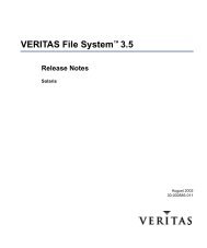
Program execution model
To clearly examine the performance characteristics of a workload, a dynamic rather than a static model of
program execution is necessary, as shown in the following figure.
2 AIX Version 6.1 Performance management

Figure 1. Program Execution Hierarchy. The figure is a triangle on its base. The left side represents hardware entities
that are matched to the appropriate operating system entity on the right side. A program must go from the lowest level
of being stored on disk, to the highest level being the processor running program instructions. For instance, from
bottom to top, the disk hardware entity holds executable programs; real memory holds waiting operating system
threads and interrupt handlers; the translation lookaside buffer holds dispatchable threads; cache contains the
currently dispatched thread and the processor pipeline and registers contain the current instruction.
To run, a program must make its way up both the hardware and operating-system hierarchies in parallel.
Each element in the hardware hierarchy is more scarce and more expensive than the element below it.
Not only does the program have to contend with other programs for each resource, the transition from one
level to the next takes time. To understand the dynamics of program execution, you need a basic
understanding of each of the levels in the hierarchy.
Hardware hierarchy
Usually, the time required to move from one hardware level to another consists primarily of the latency of
the lower level (the time from the issuing of a request to the receipt of the first data).
Fixed disks
The slowest operation for a running program on a standalone system is obtaining code or data from a
disk, for the following reasons:
v The disk controller must be directed to access the specified blocks (queuing delay).
v The disk arm must seek to the correct cylinder (seek latency).
v The read/write heads must wait until the correct block rotates under them (rotational latency).
v The data must be transmitted to the controller (transmission time) and then conveyed to the application
program (interrupt-handling time).
Slow disk operations can have many causes besides explicit read or write requests in the program.
System-tuning activities frequently prove to be hunts for unnecessary disk I/O.
Performance management 3

Real memory
Real memory, often referred to as Random Access Memory, or RAM, is faster than disk, but much more
expensive per byte. Operating systems try to keep in RAM only the code and data that are currently in
use, storing any excess onto disk, or never bringing them into RAM in the first place.
RAM is not necessarily faster than the processor though. Typically, a RAM latency of dozens of processor
cycles occurs between the time the hardware recognizes the need for a RAM access and the time the
data or instruction is available to the processor.
If the access is going to a page of virtual memory that is stored over to disk, or has not been brought in
yet, a page fault occurs, and the execution of the program is suspended until the page has been read from
disk.
Translation Lookaside Buffer (TLB)
Programmers are insulated from the physical limitations of the system by the implementation of virtual
memory. You design and code programs as though the memory were very large, and the system takes
responsibility for translating the program’s virtual addresses for instructions and data into the real
addresses that are needed to get the instructions and data from RAM. Because this address-translation
process can be time-consuming, the system keeps the real addresses of recently accessed virtual-memory
pages in a cache called the translation lookaside buffer (TLB).
As long as the running program continues to access a small set of program and data pages, the full
virtual-to-real page-address translation does not need to be redone for each RAM access. When the
program tries to access a virtual-memory page that does not have a TLB entry, called a TLB miss, dozens
of processor cycles, called the TLB-miss latency are required to perform the address translation.
Caches
To minimize the number of times the program has to experience the RAM latency, systems incorporate
caches for instructions and data. If the required instruction or data is already in the cache, a cache hit
results and the instruction or data is available to the processor on the next cycle with no delay. Otherwise,
a cache miss occurs with RAM latency.
In some systems, there are two or three levels of cache, usually called L1, L2, and L3. If a particular
storage reference results in an L1 miss, then L2 is checked. If L2 generates a miss, then the reference
goes to the next level, either L3, if it is present, or RAM.
Cache sizes and structures vary by model, but the principles of using them efficiently are identical.
Pipeline and registers
A pipelined, superscalar architecture makes possible, under certain circumstances, the simultaneous
processing of multiple instructions. Large sets of general-purpose registers and floating-point registers
make it possible to keep considerable amounts of the program’s data in registers, rather than continually
storing and reloading the data.
The optimizing compilers are designed to take maximum advantage of these capabilities. The compilers’
optimization functions should always be used when generating production programs, however small the
programs are. The Optimization and Tuning Guide for XL Fortran, XL C and XL C++ describes how
programs can be tuned for maximum performance.
Software hierarchy
To run, a program must also progress through a series of steps in the software hierarchy.
4 AIX Version 6.1 Performance management

Executable programs
When you request a program to run, the operating system performs a number of operations to transform
the executable program on disk to a running program.
First, the directories in the your current PATH environment variable must be scanned to find the correct
copy of the program. Then, the system loader (not to be confused with the ld command, which is the
binder) must resolve any external references from the program to shared libraries.
To represent your request, the operating system creates a process, or a set of resources, such as a
private virtual address segment, which is required by any running program.
The operating system also automatically creates a single thread within that process. A thread is the current
execution state of a single instance of a program. In AIX, access to the processor and other resources is
allocated on a thread basis, rather than a process basis. Multiple threads can be created within a process
by the application program. Those threads share the resources owned by the process within which they
are running.
Finally, the system branches to the entry point of the program. If the program page that contains the entry
point is not already in memory (as it might be if the program had been recently compiled, executed, or
copied), the resulting page-fault interrupt causes the page to be read from its backing storage.
Interrupt handlers
The mechanism for notifying the operating system that an external event has taken place is to interrupt the
currently running thread and transfer control to an interrupt handler.
Before the interrupt handler can run, enough of the hardware state must be saved to ensure that the
system can restore the context of the thread after interrupt handling is complete. Newly invoked interrupt
handlers experience all of the delays of moving up the hardware hierarchy (except page faults). Unless the
interrupt handler was run very recently (or the intervening programs were very economical), it is unlikely
that any of its code or data remains in the TLBs or the caches.
When the interrupted thread is dispatched again, its execution context (such as register contents) is
logically restored, so that it functions correctly. However, the contents of the TLBs and caches must be
reconstructed on the basis of the program’s subsequent demands. Thus, both the interrupt handler and the
interrupted thread can experience significant cache-miss and TLB-miss delays as a result of the interrupt.
Waiting threads
Whenever an executing program makes a request that cannot be satisfied immediately, such as a
synchronous I/O operation (either explicit or as the result of a page fault), that thread is put in a waiting
state until the request is complete.
Normally, this results in another set of TLB and cache latencies, in addition to the time required for the
request itself.
Dispatchable threads
When a thread is dispatchable but not running, it is accomplishing nothing useful. Worse, other threads
that are running may cause the thread’s cache lines to be reused and real memory pages to be reclaimed,
resulting in even more delays when the thread is finally dispatched.
Currently dispatched threads
The scheduler chooses the thread that has the strongest claim to the use of the processor.
The considerations that affect that choice are discussed in “Processor scheduler performance” on page 31.
When the thread is dispatched, the logical state of the processor is restored to the state that was in effect
when the thread was interrupted.
Performance management 5

Current machine instructions
Most of the machine instructions are capable of executing in a single processor cycle if no TLB or cache
miss occurs.
In contrast, if a program branches rapidly to different areas of the program and accesses data from a large
number of different areas causing high TLB and cache-miss rates, the average number of processor
cycles per instruction (CPI) executed might be much greater than one. The program is said to exhibit poor
locality of reference. It might be using the minimum number of instructions necessary to do its job, but it is
consuming an unnecessarily large number of cycles. In part because of this poor correlation between
number of instructions and number of cycles, reviewing a program listing to calculate path length no longer
yields a time value directly. While a shorter path is usually faster than a longer path, the speed ratio can
be very different from the path-length ratio.
The compilers rearrange code in sophisticated ways to minimize the number of cycles required for the
execution of the program. The programmer seeking maximum performance must be primarily concerned
with ensuring that the compiler has all of the information necessary to optimize the code effectively, rather
than trying to second-guess the compiler’s optimization techniques (see Effective Use of Preprocessors
and the Compilers). The real measure of optimization effectiveness is the performance of an authentic
workload.
System tuning
After efficiently implementing application programs, further improvements in the overall performance of
your system becomes a matter of system tuning.
The main components that are subject to system-level tuning are:
Communications I/O
Depending on the type of workload and the type of communications link, it might be necessary to
tune one or more of the following communications device drivers: TCP/IP, or NFS.
Fixed Disk
The Logical Volume Manager (LVM) controls the placement of file systems and paging spaces on
the disk, which can significantly affect the amount of seek latency the system experiences. The
disk device drivers control the order in which I/O requests are acted upon.
Real Memory
The Virtual Memory Manager (VMM) controls the pool of free real-memory frames and determines
when and from where to steal frames to replenish the pool.
Running Thread
The scheduler determines which dispatchable entity should next receive control. In AIX, the
dispatchable entity is a thread. See “Thread support” on page 31.
Performance tuning
Performance tuning of the system and workload is very important.
The performance-tuning process
Performance tuning is primarily a matter of resource management and correct system-parameter setting.
Tuning the workload and the system for efficient resource use consists of the following steps:
1. Identifying the workloads on the system
2. Setting objectives:
a. Determining how the results will be measured
b. Quantifying and prioritizing the objectives
6 AIX Version 6.1 Performance management

3. Identifying the critical resources that limit the system’s performance
4. Minimizing the workload’s critical-resource requirements:
a. Using the most appropriate resource, if there is a choice
b. Reducing the critical-resource requirements of individual programs or system functions
c. Structuring for parallel resource use
5. Modifying the allocation of resources to reflect priorities
a. Changing the priority or resource limits of individual programs
b. Changing the settings of system resource-management parameters
6. Repeating steps 3 through 5 until objectives are met (or resources are saturated)
7. Applying additional resources, if necessary
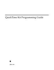
There are appropriate tools for each phase of system performance management (see “Monitoring and
tuning commands and subroutines” on page 361). Some of the tools are available from IBM ® ; others are
the products of third parties. The following figure illustrates the phases of performance management in a
simple LAN environment.
Figure 2. Performance Phases. The figure uses five weighted circles to illustrate the steps of performance tuning a
system; plan, install, monitor, tune, and expand. Each circle represents the system in various states of performance;
idle, unbalanced, balanced, and overloaded. Essentially, you expand a system that is overloaded, tune a system until
it is balanced, monitor an unbalanced system and install for more resources when an expansion is necessary.
Identification of the workloads
It is essential that all of the work performed by the system be identified. Especially in LAN-connected
systems, a complex set of cross-mounted file systems can easily develop with only informal agreement
among the users of the systems. These file systems must be identified and taken into account as part of
any tuning activity.
With multiuser workloads, the analyst must quantify both the typical and peak request rates. It is also
important to be realistic about the proportion of the time that a user is actually interacting with the terminal.
An important element of this identification stage is determining whether the measurement and tuning
activity has to be done on the production system or can be accomplished on another system (or off-shift)
with a simulated version of the actual workload. The analyst must weigh the greater authenticity of results
from a production environment against the flexibility of the nonproduction environment, where the analyst
can perform experiments that risk performance degradation or worse.
Performance management 7

Importance of setting objectives
Although you can set objectives in terms of measurable quantities, the actual desired result is often
subjective, such as satisfactory response time. Further, the analyst must resist the temptation to tune what
is measurable rather than what is important. If no system-provided measurement corresponds to the
desired improvement, that measurement must be devised.
The most valuable aspect of quantifying the objectives is not selecting numbers to be achieved, but
making a public decision about the relative importance of (usually) multiple objectives. Unless these
priorities are set in advance, and understood by everyone concerned, the analyst cannot make trade-off
decisions without incessant consultation. The analyst is also apt to be surprised by the reaction of users or
management to aspects of performance that have been ignored. If the support and use of the system
crosses organizational boundaries, you might need a written service-level agreement between the
providers and the users to ensure that there is a clear common understanding of the performance
objectives and priorities.
Identification of critical resources
In general, the performance of a given workload is determined by the availability and speed of one or two
critical system resources. The analyst must identify those resources correctly or risk falling into an endless
trial-and-error operation.
Systems have both real, logical, and possibly virtual resources. Critical real resources are generally easier
to identify, because more system performance tools are available to assess the utilization of real
resources. The real resources that most often affect performance are as follows:
v CPU cycles
v Memory
v I/O bus
v Various adapters
v Disk space
v Network access
Logical resources are less readily identified. Logical resources are generally programming abstractions that
partition real resources. The partitioning is done to share and manage the real resource.
You can use virtual resources on POWER5 -based IBM System p
systems, including
Micro-Partitioning , virtual Serial Adapter, virtual SCSI and virtual Ethernet.
Some examples of real resources and the logical and virtual resources built on them are as follows:
CPU
v Processor time slice
v CPU entitlement or Micro-Partitioning
v Virtual Ethernet
Memory
v Page frames
v Stacks
v Buffers
v Queues
v Tables
v Locks and semaphores
8 AIX Version 6.1 Performance management

Disk space
v Logical volumes
v File systems
v Files
v Logical partitions
v Virtual SCSI
Network access
v Sessions
v Packets
v Channels
v Shared Ethernet
It is important to be aware of logical and virtual resources as well as real resources. Threads can be
blocked by a lack of logical resources just as for a lack of real resources, and expanding the underlying
real resource does not necessarily ensure that additional logical resources will be created. For example,
the NFS server daemon, or nfsd daemon on the server is required to handle each pending NFS remote
I/O request. The number of nfsd daemons therefore limits the number of NFS I/O operations that can be
in progress simultaneously. When a shortage of nfsd daemons exists, system instrumentation might
indicate that various real resources, like the CPU, are used only slightly. You might have the false
impression that your system is under-used and slow, when in fact you have a shortage of nfsd daemons
which constrains the rest of the resources. A nfsd daemon uses processor cycles and memory, but you
cannot fix this problem simply by adding real memory or upgrading to a faster CPU. The solution is to
create more of the logical resource, the nfsd daemons.
Logical resources and bottlenecks can be created inadvertently during application development. A method
of passing data or controlling a device may, in effect, create a logical resource. When such resources are
created by accident, there are generally no tools to monitor their use and no interface to control their
allocation. Their existence may not be appreciated until a specific performance problem highlights their
importance.
Minimizing critical-resource requirements
Consider minimizing the workload’s critical-resource requirements at three levels.
Using the appropriate resource:
The decision to use one resource over another should be done consciously and with specific goals in
mind.
An example of a resource choice during application development would be a trade-off of increased
memory consumption for reduced CPU consumption. A common system configuration decision that
demonstrates resource choice is whether to place files locally on an individual workstation or remotely on
a server.
Reducing the requirement for the critical resource:
For locally developed applications, the programs can be reviewed for ways to perform the same function
more efficiently or to remove unnecessary function.
At a system-management level, low-priority workloads that are contending for the critical resource can be
moved to other systems, run at other times, or controlled with the Workload Manager.
Structuring for parallel use of resources:
Performance management 9

Because workloads require multiple system resources to run, take advantage of the fact that the resources
are separate and can be consumed in parallel.
For example, the operating system read-ahead algorithm detects the fact that a program is accessing a file
sequentially and schedules additional sequential reads to be done in parallel with the application’s
processing of the previous data. Parallelism applies to system management as well. For example, if an
application accesses two or more files at the same time, adding an additional disk drive might improve the
disk-I/O rate if the files that are accessed at the same time are placed on different drives.
Resource allocation priorities
The operating system provides a number of ways to prioritize activities.
Some, such as disk pacing, are set at the system level. Others, such as process priority, can be set by
individual users to reflect the importance they attach to a specific task.
Repeating the tuning steps
A truism of performance analysis is that there is always a next bottleneck. Reducing the use of one
resource means that another resource limits throughput or response time.
Suppose, for example, we have a system in which the utilization levels are as follows:
CPU: 90% Disk: 70% Memory 60%
This workload is CPU-bound. If we successfully tune the workload so that the CPU load is reduced from
90 to 45 percent, we might expect a two-fold improvement in performance. Unfortunately, the workload is
now I/O-limited, with utilizations of approximately the following:
CPU: 45% Disk: 90% Memory 60%
The improved CPU utilization allows the programs to submit disk requests sooner, but then we hit the limit
imposed by the disk drive’s capacity. The performance improvement is perhaps 30 percent instead of the
100 percent we had envisioned.
There is always a new critical resource. The important question is whether we have met the performance
objectives with the resources at hand.
Attention: Improper system tuning with the vmo, ioo, schedo, no, and nfso tuning commands might
result in unexpected system behavior like degraded system or application performance, or a system hang.
Changes should only be applied when a bottleneck has been identified by performance analysis.
Note: There is no such thing as a general recommendation for performance dependent tuning settings.
Applying additional resources
If, after all of the preceding approaches have been exhausted, the performance of the system still does not
meet its objectives, the critical resource must be enhanced or expanded.
If the critical resource is logical and the underlying real resource is adequate, the logical resource can be
expanded at no additional cost. If the critical resource is real, the analyst must investigate some additional
questions:
v How much must the critical resource be enhanced or expanded so that it ceases to be a bottleneck?
v Will the performance of the system then meet its objectives, or will another resource become saturated
first?
v If there will be a succession of critical resources, is it more cost-effective to enhance or expand all of
them, or to divide the current workload with another system?
10 AIX Version 6.1 Performance management

Performance benchmarking
When we attempt to compare the performance of a given piece of software in different environments, we
are subject to a number of possible errors, some technical, some conceptual. This section contains mostly
cautionary information. Other sections of this book discuss the various ways in which elapsed and
process-specific times can be measured.
When we measure the elapsed (wall-clock) time required to process a system call, we get a number that
consists of the following:
v The actual time during which the instructions to perform the service were executing
v Varying amounts of time during which the processor was stalled while waiting for instructions or data
from memory (that is, the cost of cache and TLB misses)
v The time required to access the clock at the beginning and end of the call
v Time consumed by periodic events, such as system timer interrupts
v Time consumed by more or less random events, such as I/O interrupts
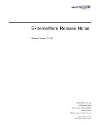
To avoid reporting an inaccurate number, we normally measure the workload a number of times. Because
all of the extraneous factors add to the actual processing time, the typical set of measurements has a
curve of the form shown in the following illustration.
Figure 3. Curve for Typical Set of Measurement.
The extreme low end may represent a low-probability optimum caching situation or may be a rounding
effect.
A regularly recurring extraneous event might give the curve a bimodal form (two maxima), as shown in the
following illustration.
Performance management 11

"Actual" value Mean
Figure 4. Bimodal Curve
One or two time-consuming interrupts might skew the curve even further, as shown in the following
illustration:
Figure 5. Skewed Curve
The distribution of the measurements about the actual value is not random, and the classic tests of
inferential statistics can be applied only with great caution. Also, depending on the purpose of the
measurement, it may be that neither the mean nor the actual value is an appropriate characterization of
performance.
System performance monitoring
AIX provides many tools and techniques for monitoring performance-related system activity.
Continuous system-performance monitoring advantages
There are several advantages to continuously monitoring system performance.
Continuous system performance monitoring can do the following:
v Sometimes detect underlying problems before they have an adverse effect
v Detect problems that affect a user’s productivity
12 AIX Version 6.1 Performance management

v Collect data when a problem occurs for the first time
v Allow you to establish a baseline for comparison
Successful monitoring involves the following:
v Periodically obtaining performance-related information from the operating system
v Storing the information for future use in problem diagnosis
v Displaying the information for the benefit of the system administrator
v Detecting situations that require additional data collection or responding to directions from the system
administrator to collect such data, or both
v Collecting and storing the necessary detail data
v Tracking changes made to the system and applications
Continuous system-performance monitoring with commands
The vmstat, iostat, netstat, and sar commands provide the basic foundation upon which you can
construct a performance-monitoring mechanism.
You can write shell scripts to perform data reduction on the command output, warn of performance
problems, or record data on the status of a system when a problem is occurring. For example, a shell
script can test the CPU idle percentage for zero, a saturated condition, and execute another shell script for
when the CPU-saturated condition occurred. The following script records the 15 active processes that
consumed the most CPU time other than the processes owned by the user of the script:
# ps -ef | egrep -v "STIME|$LOGNAME" | sort +3 -r | head -n 15
Continuous performance monitoring with the vmstat command
The vmstat command is useful for obtaining an overall picture of CPU, paging, and memory usage.
The following is a sample report produced by the vmstat command:
# vmstat 5 2
kthr memory page faults cpu
----- ----------- ------------------------ ------------ -----------
r b avm fre re pi po fr sr cy in sy cs us sy id wa
1 1 197167 477552 0 0 0 7 21 0 106 1114 451 0 0 99 0
0 0 197178 477541 0 0 0 0 0 0 443 1123 442 0 0 99 0
Remember that the first report from the vmstat command displays cumulative activity since the last
system boot. The second report shows activity for the first 5-second interval.
For detailed discussions of the vmstat command, see “vmstat command” on page 91, “Memory usage
determination with the vmstat command” on page 113, and “Assessing disk performance with the vmstat
command” on page 160.
Continuous performance monitoring with the iostat command
The iostat command is useful for determining disk and CPU usage.
The following is a sample report produced by the iostat command:
# iostat 5 2
tty: tin tout avg-cpu: % user % sys % idle % iowait
0.1 102.3 0.5 0.2 99.3 0.1
" Disk history since boot not available. "
tty: tin tout avg-cpu: % user % sys % idle % iowait
0.2 79594.4 0.6 6.6 73.7 19.2
Disks: % tm_act Kbps tps Kb_read Kb_wrtn
Performance management 13

hdisk1 0.0 0.0 0.0 0 0
hdisk0 78.2 1129.6 282.4 5648 0
cd1 0.0 0.0 0.0 0 0
Remember that the first report from the iostat command shows cumulative activity since the last system
boot. The second report shows activity for the first 5-second interval.
The system maintains a history of disk activity. In the example above, you can see that the history is
disabled by the appearance of the following message:
Disk history since boot not available.
To disable or enable disk I/O history with smitty, type the following at the command line:
# smitty chgsys
Continuously maintain DISK I/O history [value]
and set the value to either false to disable disk I/O history or true to enable disk I/O history. The interval
disk I/O statistics are unaffected by this setting.
For detailed discussion of the iostat command, see “The iostat command” on page 93 and “Assessing
disk performance with the iostat command” on page 158.
Continuous performance monitoring with the netstat command
The netstat command is useful in determining the number of sent and received packets.
The following is a sample report produced by the netstat command:
# netstat -I en0 5
input (en0) output input (Total) output
packets errs packets errs colls packets errs packets errs colls
8305067 0 7784711 0 0 20731867 0 20211853 0 0
3 0 1 0 0 7 0 5 0 0
24 0 127 0 0 28 0 131 0 0
CTRL C
Remember that the first report from the netstat command shows cumulative activity since the last system
boot. The second report shows activity for the first 5-second interval.
Other useful netstat command options are -s and -v. For details, see “netstat command” on page 266.
Continuous performance monitoring with the sar command
The sar command is useful in determining CPU usage.
The following is a sample report produced by the sar command:
# sar -P ALL 5 2
AIX aixhost 2 5 00040B0F4C00 01/29/04
10:23:15 cpu %usr %sys %wio %idle
10:23:20 0 0 0 1 99
1 0 0 0 100
2 0 1 0 99
3 0 0 0 100
- 0 0 0 99
10:23:25 0 4 0 0 96
1 0 0 0 100
2 0 0 0 100
3 3 0 0 97
- 2 0 0 98
Average 0 2 0 0 98
14 AIX Version 6.1 Performance management

1 0 0 0 100
2 0 0 0 99
3 1 0 0 99
- 1 0 0 99
The sar command does not report the cumulative activity since the last system boot.
For details on the sar command, see “The sar command” on page 94 and “Assessing disk performance
with the sar command” on page 161.
Continuous system-performance monitoring with the topas command
The topas command reports vital statistics about the activity on the local system, such as real memory
size and the number of write system calls.
The topas command uses the curses library to display its output in a format suitable for viewing on an
80x25 character-based display or in a window of at least the same size on a graphical display. The topas
command extracts and displays statistics from the system with a default interval of two seconds. The
topas command offers the following alternate screens:
v Overall system statistics
v List of busiest processes
v WLM statistics
v List of hot physical disks
v Logical partition display
v Cross-Partition View (AIX 5.3 with 5300-03 and higher)
The bos.perf.tools fileset and the perfagent.tools fileset must be installed on the system to run the
topas command.
For more information on the topas command, see the topas command in AIX Version 6.1 Commands
Reference, Volume 5.
The overall system statistics screen
The output of the overall system statistics screen consists of one fixed section and one variable section.
The top two lines at the left of the output shows the name of the system that the topas program is running
on, the date and time of the last observation, and the monitoring interval. Below this section is a variable
section which lists the following subsections:
v CPU utilization
v Network interfaces
v Physical disks
v WLM classes
v Processes
To the right of this section is the fixed section which contains the following subsections of statistics:
v EVENTS/QUEUES
v FILE/TTY
v PAGING
v MEMORY
v PAGING SPACE
v NFS
The following is a sample output of the overall system statistics screen:
Performance management 15

Topas Monitor for host: aixhost EVENTS/QUEUES FILE/TTY
Wed Feb 4 11:23:41 2004 Interval: 2 Cswitch 53 Readch 6323
Syscall 152 Writech 431
Kernel 0.0 | | Reads 3 Rawin 0
User 0.9 | | Writes 0 Ttyout 0
Wait 0.0 | | Forks 0 Igets 0
Idle 99.0 |############################| Execs 0 Namei 10
Runqueue 0.0 Dirblk 0
Network KBPS I-Pack O-Pack KB-In KB-Out Waitqueue 0.0
en0 0.8 0.4 0.9 0.0 0.8
lo0 0.0 0.0 0.0 0.0 0.0 PAGING MEMORY
Faults 2 Real,MB 4095
Disk Busy% KBPS TPS KB-Read KB-Writ Steals 0 % Comp 8.0
hdisk0 0.0 0.0 0.0 0.0 0.0 PgspIn 0 % Noncomp 15.8
hdisk1 0.0 0.0 0.0 0.0 0.0 PgspOut 0 % Client 14.7
PageIn 0
WLM-Class (Active) CPU% Mem% Disk-I/O% PageOut 0 PAGING SPACE
System 0 0 0 Sios 0 Size,MB 512
Shared 0 0 0 % Used 1.2
Default 0 0 0 NFS (calls/sec) % Free 98.7
Name PID CPU% PgSp Class 0 ServerV2 0
topas 10442 3.0 0.8 System ClientV2 0 Press:
ksh 13438 0.0 0.4 System ServerV3 0 "h" for help
gil 1548 0.0 0.0 System ClientV3 0 "q" to quit
Except for the variable Processes subsection, you can sort all of the subsections by any column by
moving the cursor to the top of the desired column. All of the variable subsections, except the Processes
subsection, have the following views:
v List of top resource users
v One-line report presenting the sum of the activity
For example, the one-line-report view might show just the total disk or network throughput.
For the CPU subsection, you can select either the list of busy processors or the global CPU utilization, as
shown in the above example.
List of busiest processes screen of the topas monitor
To view the screen that lists the busiest processes, use the -P flag of the topas command.
This screen is similar to the Processes subsection of the overall system statistics screen, but with
additional detail. You can sort this screen by any of the columns by moving the cursor to the top of the
desired column. The following is an example of the output of the busiest processes screen:
Topas Monitor for host: aixhost Interval: 2 Wed Feb 4 11:24:05 2004
DATA TEXT PAGE PGFAULTS
USER PID PPID PRI NI RES RES SPACE TIME CPU% I/O OTH COMMAND
root 1 0 60 20 202 9 202 0:04 0.0 111 1277 init
root 774 0 17 41 4 0 4 0:00 0.0 0 2 reaper
root 1032 0 60 41 4 0 4 0:00 0.0 0 2 xmgc
root 1290 0 36 41 4 0 4 0:01 0.0 0 530 netm
root 1548 0 37 41 17 0 17 1:24 0.0 0 23 gil
root 1806 0 16 41 4 0 4 0:00 0.0 0 12 wlmsched
root 2494 0 60 20 4 0 4 0:00 0.0 0 6 rtcmd
root 2676 1 60 20 91 10 91 0:00 0.0 20 6946 cron
root 2940 1 60 20 171 22 171 0:00 0.0 15 129 errdemon
root 3186 0 60 20 4 0 4 0:00 0.0 0 125 kbiod
root 3406 1 60 20 139 2 139 1:23 0.0 1542187 syncd
root 3886 0 50 41 4 0 4 0:00 0.0 0 2 jfsz
root 4404 0 60 20 4 0 4 0:00 0.0 0 2 lvmbb
root 4648 1 60 20 17 1 17 0:00 0.0 1 24 sa_daemon
root 4980 1 60 20 97 13 97 0:00 0.0 37 375 srcmstr
root 5440 1 60 20 15 2 15 0:00 0.0 7 28 shlap
root 5762 1 60 20 4 0 4 0:00 0.0 0 2 random
16 AIX Version 6.1 Performance management

oot 5962 4980 60 20 73 10 73 0:00 0.0 22 242 syslogd
root 6374 4980 60 20 63 2 63 0:00 0.0 2 188 rpc.lockd
root 6458 4980 60 20 117 12 117 0:00 0.0 54 287 portmap
WLM statistics screen of the topas monitor
To view the screen that shows the WLM statistics, use the -W flag of the topas command.
This screen is divided into the following sections:
v The top section is the list of busiest WLM classes, as presented in the WLM subsection of the overall
system statistics screen, which you can also sort by any of the columns.
v The second section of this screen is a list of hot processes within the WLM class you select by using
the arrow keys or the f key.
The following is an example of the WLM full screen report:
Topas Monitor for host: aixhost Interval: 2 Wed Feb 4 11:24:29 2004
WLM-Class (Active) CPU% Mem% Disk-I/O%
System 0 0 0
Shared 0 0 0
Default 0 0 0
Unmanaged 0 0 0
Unclassified 0 0 0
==============================================================================
DATA TEXT PAGE PGFAULTS
USER PID PPID PRI NI RES RES SPACE TIME CPU% I/O OTH COMMAND
root 1 0 60 20 202 9 202 0:04 0.0 0 0 init
root 774 0 17 41 4 0 4 0:00 0.0 0 0 reaper
root 1032 0 60 41 4 0 4 0:00 0.0 0 0 xmgc
root 1290 0 36 41 4 0 4 0:01 0.0 0 0 netm
root 1548 0 37 41 17 0 17 1:24 0.0 0 0 gil
root 1806 0 16 41 4 0 4 0:00 0.0 0 0 wlmsched
root 2494 0 60 20 4 0 4 0:00 0.0 0 0 rtcmd
root 2676 1 60 20 91 10 91 0:00 0.0 0 0 cron
root 2940 1 60 20 171 22 171 0:00 0.0 0 0 errdemon
root 3186 0 60 20 4 0 4 0:00 0.0 0 0 kbiod
Viewing the physical disks screen
To view the screen that shows the list of hot physical disks, use the -D flag with the topas command.
The maximum number of physical disks displayed is the number of hot physical disks being monitored as
specified with the -d flag. The list of hot physical disks is sorted by the KBPS field.
The following is an example of the report generated by the topas -D command:
Topas Monitor for host: aixcomm Interval: 2 Fri Jan 13 18:00:16 XXXX
===============================================================================
Disk Busy% KBPS TPS KB-R ART MRT KB-W AWT MWT AQW AQD
hdisk0 3.0 56.0 3.5 0.0 0.0 5.4 56.0 5.8 33.2 0.0 0.0
cd0 0.0 0.0 0.0 0.0 0.0 0.0 0.0 0.0 0.0 0.0 0.0
For more information on the topas-D command, see the topas command in AIX Version 6.1 Commands
Reference, Volume 5.
Viewing the Cross-Partition panel
To view cross-partition statistics in topas, use the -C flag with the topas command or press the C key
from any other panel.
The screen is divided into the following sections:
Performance management 17

v The top section displays aggregated data from the partition set to show overall partition, memory, and
processor activity. The G key toggles this section between brief listing, detailed listing, and off.
v The bottom section displays the per partition statistics, which are in turn divided into two sections:
shared partitions and dedicated partitions. The S key toggles the shared partition section on and off.
The D key toggles the dedicated partition section on and off.
The following is a full screen example of the output from the topas -C command:
Topas CEC Monitor Interval: 10 Wed Mar 6 14:30:10 XXXX
Partitions Memory (GB) Processors
Shr: 4 Mon: 24 InUse: 14 Mon: 8 PSz: 4 Shr_PhysB: 1.7
Ded: 4 Avl: 24 Avl: 8 APP: 4 Ded_PhysB: 4.1
Host OS M Mem InU Lp Us Sy Wa Id PhysB Ent %EntC Vcsw PhI
--------------------------------shared------------------------------------------
ptools1 A53 u 1.1 0.4 4 15 3 0 82 1.30 0.50 22.0 200 5
ptools5 A53 U 12 10 1 12 3 0 85 0.20 0.25 0.3 121 3
ptools3 A53 C 5.0 2.6 1 10 1 0 89 0.15 0.25 0.3 52 2
ptools7 A53 c 2.0 0.4 1 0 1 0 99 0.05 0.10 0.3 112 2
-------------------------------dedicated----------------------------------------
ptools4 A53 S 0.6 0.3 2 12 3 0 85 0.60
ptools6 A52 1.1 0.1 1 11 7 0 82 0.50
ptools8 A52 1.1 0.1 1 11 7 0 82 0.50
ptools2 A52 1.1 0.1 1 11 7 0 82 0.50
Partitions can be sorted by any column except Host, OS, and M, by moving the cursor to the top of the
desired column.
For more information on the topas -C command, see the topas command in AIX Version 6.1 Commands
Reference, Volume 5.
Viewing local logical partition-level information
To view partition-level information and per-logical-processor performance metrics, use the -L flag with the
topas command or press the L key from any other panel.
The screen is divided into two sections:
v The upper section displays a subset of partition-level information.
v The lower section displays a sorted list of logical processor metrics.
The following is an example of the output from the topas -L command:
Interval: 2 Logical Partition: aix Sat Mar 13 09:44:48 XXXX
Poolsize: 3.0 Shared SMT ON Online Memory: 8192.0
Entitlement: 2.5 Mode: Capped Online Logical CPUs: 4
Online Virtual CPUs: 2
%user %sys %wait %idle physc %entc %lbusy app vcsw phint %hypv hcalls
47.5 32.5 7.0 13.0 2.0 80.0 100.0 1.0 240 150 5.0 1500
==============================================================================
logcpu minpf majpf intr csw icsw runq lpa scalls usr sys wt idl pc lcsw
cpu0 1135 145 134 78 60 2 95 12345 10 65 15 10 0.6 120
cpu1 998 120 104 92 45 1 89 4561 8 67 25 0 0.4 120
cpu2 2246 219 167 128 72 3 92 76300 20 50 20 10 0.5 120
cpu3 2167 198 127 62 43 2 94 1238 18 45 15 22 0.5 120
For more information on the topas-L command, see the topas command in AIX Version 6.1 Commands
Reference, Volume 5.
SMIT panels for topas/topasout
SMIT panels are available for easier configuration and setup of the topas recording function and report
generation.
18 AIX Version 6.1 Performance management

To go to the topas smit panel, type smitty performance (or smitty topas) and select Configure Topas
options.
The Configure Topas Options menu displays:
Configure Topas Options
Move cursor to desired item and press Enter
Add Host to topas external subnet search file (Rsi.hosts)
List hosts in topas external subnet search file (Rsi.hosts)
Configure Recordings
List Available Recordings
Show current recordings status
Generate Report
For more information, see the topas command in AIX Version 6.1 Commands Reference, Volume 5.
Adding a host to the topas external subnet search file (Rsi.hosts):
The PTX ®
clients and topas -C|-R command are limited in that the Remote Statistics Interface (RSi) API
used to identify remote hosts.
Whenever a client is started, it broadcasts a query on the xmquery port which is a registered service of
the inetd daemon. Remote hosts see this query and the inetd.conf file is configured to start the xmservd
or xmtopas daemons and reply to the querying client. The existing architecture limits the xmquery call to
within hosts residing on the same subnet as the system making the query.
To get around this problem, PTX has always supported user-customized host lists that reside outside the
subnet. The RSi reads this host list (RSi.hosts file), and directly polls any hostname or IP listed. You can
customize RSi.hosts file. By default, the RSi searches the following locations in order of precedence:
1. $HOME/Rsi.hosts
2. /etc/perf/Rsi.hosts
3. /usr/lpp/perfmgr/Rsi.hosts
This files format lists one host per entry line, either by Internet Address format or fully-qualified hostname,
as in the following example:
ptoolsl1.austin.ibm.com
9.3.41.206
...
Select the Add Host to topas external subnet search file (Rsi.hosts) option to add hosts to the
Rsi.hosts file. Select the List hosts in topas external subnet search file (Rsi.hosts) option to see the
list of options in the Rsi.hosts file.
Configuring recordings:
You can use the Configure Recordings option in the Configure Topas Options menu to enable or disable
recordings.
Select from the following menu options to configure recordings:
Configure Recordings
Move cursor to desired item and press Enter.
Enable CEC recording
Disable CEC recording
Enable local recording
Disable local recording
Performance management 19

Option Description
Enable CEC recording Selecting this option starts the topas CEC recording.
Disable CEC recording Selecting this option terminates the topas CEC recording session. The
script does not provide an error check If you try to start topas when it is
already running, no action is done.
Enable local recording Selecting this option enables daily, as well as IBM Workload Estimator
(WLE), recordings and starts the xmwlm recording. The WLE report is
generated only on Sundays and requires local recording to always be
enabled for consistent data in the report. Enabling the WLE report
generates a weekly report on Sundays at 00:45 am. The data in the weekly
report is correct only if the local recordings are always enabled.
The generated WLE report is stored in the /etc/perf/
_aixwle_weekly.xml file. For example, if the hostname is
ptoolsl1, the weekly report is written to the /etc/perf/
ptoolsl1_aixwle_weekly.xml file.
Disable local recording Selecting this option disables both daily and WLE recordings.
Listing available recordings:
You can use the List Available Recordings option in the Configure Topas Options menu to list
information about the existing recording files in the /etc/perf and /etc/perf/daily directories.
The List Available Recordings option lists the type, date, beginning time, and ending time of all the
recordings available as shown in the following example:
Type Date Start Stop
Local 06/08/26 14:49:06 23:59:24
Local 06/08/27 00:01:06 13:09:51
CEC 06/08/20 08:45:37 09:07:54
Show current recordings status:
You can use the Show current recordings status option in the Configure Topas Options menu to see the
enablement status of the different type of recordings (CEC, Daily, and WLE) before trying to enable or
disable any recording.
The following is an example of using the Show current recordings status option:
Recording Status
========= ======
CEC Not Enabled
Local Enabled
WLE Enabled
Generating reports from existing recording files:
You can use the Generate Report option in the Configure Topas Options menu to generate reports from
the existing recording files created by daily and topas recordings in the /etc/perf or /etc/perf/daily
directories.
Using the Generate Report option prompts you to enter the values of the recording file, reporting format
(comma-separated, spreadsheet, nmon, or detailed), begin time, end time, interval, and the file/printer
name to generate a report based on the input.
Perform the following steps to generate a report:
1. Select the filename or printer to send the report to:
20 AIX Version 6.1 Performance management

Send report to File/Printer
Move cursor to desired item and press Enter.
1 Filename
2 Printer
2. Select the type and day of recording from the list of available recordings:
* Type and Day of Recording (Ex: CEC-YY/MM/DD) [] +
3. Select the reporting format (based on your type and day of recording selection):
* Reporting Format [] +
A dialog screen with your selections is displayed.
The following is an example of a comma separated/spreadsheet report type:
* Type and Day of Recording (Ex: CEC-YY/MM/DD) []
* Reporting Format []
Type [mean] +
* Output File []
The following is an example of a nmon report type:
* Type and Day of Recording (Ex: CEC-YY/MM/DD) []
* Reporting Format []
* Output File []
Note: The Output file field is mandatory for comma separated/spreadsheet, and nmon types and optional
for all other reporting formats. The topas recordings support only mean type for comma separated
and spreadsheet reporting formats.
The following is an example of a summary/disk summary/detailed/network summary report type:
* Type and Day of Recording (Ex: CEC-YY/MM/DD) []
* Reporting Format []
Begin Time (HHMM) [] +
End Time (HHMM) [] +
Interval [5] + +
Output File (defaults to stdout) []
For all the above examples, the first two fields are non-modifiable and filled with values from the previous
selections.
If printer is selected as the report output, the Output File field is replaced with the required Printer Name
field from a list of printers configured in the system:
* Printer Name [ ] +
Continuous system-performance monitoring with the Performance
Toolbox
The Performance Toolbox (PTX) is a licensed product that graphically displays a variety of
performance-related metrics.
One of the prime advantages of PTX is that you can check current system performance by taking a glance
at the graphical display rather than looking at a screen full of numbers. PTX also facilitates the compilation
of information from multiple performance-related commands and allows the recording and playback of
data.
PTX contains tools for local and remote system-activity monitoring and tuning. The PTX tools that are best
suited for continuous monitoring are the following:
Performance management 21

v The ptxrlog command produces recordings in ASCII format, which allows you to either print the output
or post-process it. You can also use the ptxrlog command to produce a recording file in binary that can
be viewed with the azizo or xmperf commands.
v The xmservd daemon acts as a recording facility and is controlled through the xmservd.cf
configuration file. This daemon simultaneously provides near real-time network-based data monitoring
and local recording on a given node.
v The xmtrend daemon, much like the xmservd daemon, acts as a recording facility. The main difference
between the xmtrend daemon and the xmservd daemon is in the storage requirements for each
daemon. Typically, the xmservd daemon recordings can consume several megabytes of disk storage
every hour. The xmtrend daemon provides manageable and perpetual recordings of large metric sets.
v The jazizo tool is a Java
version of the azizo command. The jazizo command is a tool for analyzing
the long-term performance characteristics of a system. It analyzes recordings created by the xmtrend
daemon and provides displays of the recorded data that can be customized.
v The wlmperf tools provide graphical views of Workload Manager (WLM) resource activities by class.
This tool can generate reports from trend recordings made by the PTX daemons covering a period of
minutes, hours, days, weeks, or months.
For more information about PTX, see Performance Toolbox Version 2 and 3 for AIX: Guide and Reference
and Customizing Performance Toolbox and Performance Toolbox Extensions for AIX.
Initial performance diagnosis
There are many types of reported performance problems to consider when diagnosing performance
problems.
Types of reported performance problems
When a performance problem is reported, it is helpful to determine the kind of performance problem by
narrowing the list of possibilities.
A particular program runs slowly
A program may start to run slowly for any one of several reasons.
Although this situation might seem trivial, there are still questions to answer:
v Has the program always run slowly?
If the program has just started running slowly, a recent change might be the cause.
v Has the source code changed or a new version installed?
If so, check with the programmer or vendor.
v Has something in the environment changed?
If a file used by the program, including its own executable program, has been moved, it may now be
experiencing network delays that did not exist previously. Or, files may be contending for a single-disk
accessor that were on different disks previously.
If the system administrator changed system-tuning parameters, the program may be subject to
constraints that it did not experience previously. For example, if the system administrator changed the
way priorities are calculated, programs that used to run rather quickly in the background may now be
slowed down, while foreground programs have sped up.
v Is the program written in the perl, awk, csh, or some other interpretive language?
Unfortunately, interpretive languages are not optimized by a compiler. Also, it is easy in a language like
perl or awk to request an extremely compute- or I/O-intensive operation with a few characters. It is
often worthwhile to perform a desk check or informal peer review of such programs with the emphasis
on the number of iterations implied by each operation.
v Does the program always run at the same speed or is it sometimes faster?
22 AIX Version 6.1 Performance management

The file system uses some of system memory to hold pages of files for future reference. If a disk-limited
program is run twice in quick succession, it will normally run faster the second time than the first.
Similar behavior might be observed with programs that use NFS. This can also occur with large
programs, such as compilers. The program’s algorithm might not be disk-limited, but the time needed to
load a large executable program might make the first execution of the program much longer than
subsequent ones.
v If the program has always run slowly, or has slowed down without any obvious change in its
environment, look at its dependency on resources.
Performance-limiting resource identification describes techniques for finding the bottleneck.
Everything runs slowly at a particular time of day
There are several reasons why the system may slow down at certain times of the day.
Most people have experienced the rush-hour slowdown that occurs because a large number of people in
the organization habitually use the system at one or more particular times each day. This phenomenon is
not always simply due to a concentration of load. Sometimes it is an indication of an imbalance that is only
a problem when the load is high. Other sources of recurring situations in the system should be considered.
v If you run the iostat and netstat commands for a period that spans the time of the slowdown, or if you
have previously captured data from your monitoring mechanism, are some disks much more heavily
used than others? Is the CPU idle percentage consistently near zero? Is the number of packets sent or
received unusually high?
– If the disks are unbalanced, see “Logical volume and disk I/O performance” on page 156.
– If the CPU is saturated, use the ps or topas commands to identify the programs being run during
this period. The sample script given in “Continuous system-performance monitoring with commands”
on page 13 simplifies the search for the heaviest CPU users.
– If the slowdown is counter-intuitive, such as paralysis during lunch time, look for a pathological
program such as a graphic xlock or game program. Some versions of the xlock program are known
to use huge amounts of CPU time to display graphic patterns on an idle display. It is also possible
that someone is running a program that is a known CPU burner and is trying to run it at the least
intrusive time.
v Unless your /var/adm/cron/cron.allow file is null, you may want to check the contents of the
/var/adm/cron/crontab directory for expensive operations.
If you find that the problem stems from conflict between foreground activity and long-running,
CPU-intensive programs that are, or should be, run in the background, consider changing the way
priorities are calculated using the schedo command to give the foreground higher priority. See
“Thread-Priority-Value calculation” on page 109.
Everything runs slowly at unpredictable times
The best tool for this situation is an overload detector, such as the filtd daemon, a component of PTX.
The filtd daemon can be set up to execute shell scripts or collect specific information when a particular
condition is detected. You can construct a similar, but more specialized, mechanism using shell scripts
containing the vmstat, iostat, netstat, sar, and ps commands.
If the problem is local to a single system in a distributed environment, there is probably a pathological
program at work, or perhaps two that intersect randomly.
Everything that an individual user runs is slow
Sometimes a system seems to affect a particular individual.
v The solution in this case is to quantify the problem. Ask the user which commands they use frequently,
and run those commands with the time command, as in the following example:
Performance management 23

# time cp .profile testjunk
real 0m0.08s
user 0m0.00s
sys 0m0.01s
Then run the same commands under a user ID that is not experiencing performance problems. Is there
a difference in the reported real time?
v A program should not show much CPU time (user+sys) difference from run to run, but may show a real
time difference because of more or slower I/O. Are the user’s files on an NFS-mounted directory? Or on
a disk that has high activity for other reasons?
v Check the user’s .profile file for unusual $PATH specifications. For example, if you always search a few
NFS-mounted directories before searching /usr/bin, everything will take longer.
A number of LAN-connected systems slow down simultaneously
There are some common problems that arise in the transition from independent systems to distributed
systems.
The problems usually result from the need to get a new configuration running as soon as possible, or from
a lack of awareness of the cost of certain functions. In addition to tuning the LAN configuration in terms of
maximum transmission units (MTU) and mbufs, look for LAN-specific pathologies or nonoptimal situations
that may have evolved through a sequence of individually reasonable decisions.
v Use network statistics to ensure that there are no physical network problems. Ensure that commands
such as netstat -v, entstat, tokstat, atmstat, or fddistat do not show excessive errors or collision on
the adapter.
v Some types of software or firmware bugs can sporadically saturate the LAN with broadcast or other
packets.
When a broadcast storm occurs, even systems that are not actively using the network can be slowed by
the incessant interrupts and by the CPU resource consumed in receiving and processing the packets.
These problems are better detected and localized with LAN analysis devices than with the normal
performance tools.
v Do you have two LANs connected through a system?
Using a system as a router consumes large amounts of CPU time to process and copy packets. It is
also subject to interference from other work being processed by the system. Dedicated hardware
routers and bridges are usually a more cost-effective and robust solution.
v Is there a clear purpose for each NFS mount?
At some stages in the development of distributed configurations, NFS mounts are used to give users on
new systems access to their home directories on their original systems. This situation simplifies the
initial transition, but imposes a continuing data communication cost. It is not unknown to have users on
system A interacting primarily with data on system B and vice versa.
Access to files through NFS imposes a considerable cost in LAN traffic, client and server CPU time, and
end-user response time. A general guideline is that user and data should normally be on the same
system. The exceptions are those situations in which an overriding concern justifies the extra expense
and time of remote data. Some examples are a need to centralize data for more reliable backup and
control, or a need to ensure that all users are working with the most current version of a program.
If these and other needs dictate a significant level of NFS client-server interchange, it is better to
dedicate a system to the role of server than to have a number of systems that are part-server,
part-client.
v Have programs been ported correctly and justifiably to use remote procedure calls (RPCs)?
The simplest method of porting a program into a distributed environment is to replace program calls with
RPCs on a 1:1 basis. Unfortunately, the disparity in performance between local program calls and RPCs
is even greater than the disparity between local disk I/O and NFS I/O. Assuming that the RPCs are
really necessary, they should be batched whenever possible.
24 AIX Version 6.1 Performance management

Everything on a particular service or device slows down at times
There are a variety of reasons why everything on a particular service or device slows down at times.
If everything that uses a particular device or service slows down at times, refer to the topic that covers that
particular device or service:
v “Microprocessor performance” on page 91
v “Memory performance” on page 113
v “Logical volume and disk I/O performance” on page 156
v “File system performance” on page 208
v “Network performance analysis” on page 264
v “NFS performance monitoring and tuning” on page 302
Everything runs slowly when connected remotely
Local and remote authentication to a system can behave very differently. By default, the local
authentication files are consulted first when a user logs in with their user id. This has a faster response
time than network-based authentication mechanisms.
If a user logs in and authenticates with some kind of network-authentication mechanism, that will be the
first mechanism searched when looking up user ids. This will affect any command that performs lookups of
user login names. It will also impact the following commands:
v ps -ef
v ls -l
v ipcs -a
The specific authentication programs are defined in the /usr/lib/security/methods.cfg file. The default
value is compat, which is the local authentication method. To view your current authentication setting for a
particular user id, login with the user id and at the command line, type:
# echo $AUTHSTATE
If you want to ensure that you are using a local authentication mechanism first and then the
network-based authentication mechanism, like DCE for example, type the following at the command line:
# export AUTHSTATE="compat,DCE"
Performance-Limiting Resource identification
The best tool for an overall look at resource utilization while running a multiuser workload is the vmstat
command.
The vmstat command reports CPU and disk-I/O activity, as well as memory utilization data. The following
instantiation of the vmstat command produces a one-line summary report of system activity every 5
seconds:
# vmstat 5
In the example above, because there is no count specified following the interval, reporting continues until
you cancel the command.
The following vmstat report was created on a system running AIXwindows and several synthetic
applications (some low-activity intervals have been removed for example purposes):
kthr memory page faults cpu
----- ----------- ------------------------ ------------ -----------
r b avm fre re pi po fr sr cy in sy cs us sy id wa
0 0 8793 81 0 0 0 1 7 0 125 42 30 1 2 95 2
0 0 8793 80 0 0 0 0 0 0 155 113 79 14 8 78 0
0 0 8793 57 0 3 0 0 0 0 178 28 69 1 12 81 6
Performance management 25

0 0 9192 66 0 0 16 81 167 0 151 32 34 1 6 77 16
0 0 9193 65 0 0 0 0 0 0 117 29 26 1 3 96 0
0 0 9193 65 0 0 0 0 0 0 120 30 31 1 3 95 0
0 0 9693 69 0 0 53 100 216 0 168 27 57 1 4 63 33
0 0 9693 69 0 0 0 0 0 0 134 96 60 12 4 84 0
0 0 10193 57 0 0 0 0 0 0 124 29 32 1 3 94 2
0 0 11194 64 0 0 38 201 1080 0 168 29 57 2 8 62 29
0 0 11194 63 0 0 0 0 0 0 141 111 65 12 7 81 0
0 0 5480 755 3 1 0 0 0 0 154 107 71 13 8 78 2
0 0 5467 5747 0 3 0 0 0 0 167 39 68 1 16 79 5
0 1 4797 5821 0 21 0 0 0 0 191 192 125 20 5 42 33
0 1 3778 6119 0 24 0 0 0 0 188 170 98 5 8 41 46
0 0 3751 6139 0 0 0 0 0 0 145 24 54 1 10 89 0
In this initial assessment, pay particular attention to the pi and po columns of the page category and the
four columns in the cpu category.
The pi and po entries represent the paging-space page-ins and page-outs, respectively. If you observe any
instances of paging-space I/O, the workload may be approaching or beyond the system’s memory limits.
If the sum of the user and system CPU-utilization percentages, us and sy, is greater than 90 percent in a
given 5-second interval, the workload is approaching the CPU limits of the system during that interval.
If the I/O wait percentage, wa, is close to zero and the pi and po values are zero, the system is spending
time waiting on non-overlapped file I/O, and some part of the workload is I/O-limited.
If the vmstat command indicates a significant amount of I/O wait time, use the iostat command to gather
more detailed information.
The following instantiation of the iostat command produces summary reports of I/O activity and CPU
utilization every 5 seconds, and because we specify a count of 3 following the interval, reporting will stop
after the third report:
# iostat 5 3
The following iostat report was created on a system running the same workload as the one in the vmstat
example above, but at a different time. The first report represents the cumulative activity since the
preceding boot, while subsequent reports represent the activity during the preceding 5-second interval:
tty: tin tout avg-cpu: % user % sys % idle %iowait
0.0 4.3 0.2 0.6 98.8 0.4
Disks: % tm_act Kbps tps Kb_read Kb_wrtn
hdisk0 0.0 0.2 0.0 7993 4408
hdisk1 0.0 0.0 0.0 2179 1692
hdisk2 0.4 1.5 0.3 67548 59151
cd0 0.0 0.0 0.0 0 0
tty: tin tout avg-cpu: % user % sys % idle %iowait
0.0 30.3 8.8 7.2 83.9 0.2
Disks: % tm_act Kbps tps Kb_read Kb_wrtn
hdisk0 0.2 0.8 0.2 4 0
hdisk1 0.0 0.0 0.0 0 0
hdisk2 0.0 0.0 0.0 0 0
cd0 0.0 0.0 0.0 0 0
tty: tin tout avg-cpu: % user % sys % idle %iowait
0.0 8.4 0.2 5.8 0.0 93.8
Disks: % tm_act Kbps tps Kb_read Kb_wrtn
hdisk0 0.0 0.0 0.0 0 0
26 AIX Version 6.1 Performance management

hdisk1 0.0 0.0 0.0 0 0
hdisk2 98.4 575.6 61.9 396 2488
cd0 0.0 0.0 0.0 0 0
The first report shows that the I/O on this system is unbalanced. Most of the I/O (86.9 percent of kilobytes
read and 90.7 percent of kilobytes written) goes to hdisk2, which contains both the operating system and
the paging space. The cumulative CPU utilization since boot statistic is usually meaningless, unless you
use the system consistently, 24 hours a day.
The second report shows a small amount of disk activity reading from hdisk0, which contains a separate
file system for the system’s primary user. The CPU activity arises from two application programs and the
iostat command itself.
In the third report, you can see that we artificially created a near-thrashing condition by running a program
that allocates and stores a large amount of memory, which is about 26 MB in the above example. Also in
the above example, hdisk2 is active 98.4 percent of the time, which results in 93.8 percent I/O wait.
The limiting factor for a single program
If you are the sole user of a system, you can get a general idea of whether a program is I/O or CPU
dependent by using the time command as follows:
# time cp foo.in foo.out
real 0m0.13s
user 0m0.01s
sys 0m0.02s
Note: Examples of the time command use the version that is built into the Korn shell, ksh. The official
time command, /usr/bin/time, reports with a lower precision.
In the above example, the fact that the real elapsed time for the execution of the cp program (0.13
seconds) is significantly greater than the sum (.03 seconds) of the user and system CPU times indicates
that the program is I/O bound. This occurs primarily because the foo.in file has not been read recently.
On an SMP, the output takes on a new meaning. See “Considerations of the time and timex commands”
on page 99 for more information.
Running the same command a few seconds later against the same file gives the following output:
real 0m0.06s
user 0m0.01s
sys 0m0.03s
Most or all of the pages of the foo.in file are still in memory because there has been no intervening
process to cause them to be reclaimed and because the file is small compared with the amount of RAM
on the system. A small foo.out file would also be buffered in memory, and a program using it as input
would show little disk dependency.
If you are trying to determine the disk dependency of a program, you must be sure that its input is in an
authentic state. That is, if the program will normally be run against a file that has not been accessed
recently, you must make sure that the file used in measuring the program is not in memory. If, on the other
hand, a program is usually run as part of a standard sequence in which it gets its input from the output of
the preceding program, you should prime memory to ensure that the measurement is authentic. For
example, the following command would have the effect of priming memory with the pages of the foo.in
file:
# cp foo.in /dev/null
The situation is more complex if the file is large compared to RAM. If the output of one program is the
input of the next and the entire file will not fit in RAM, the second program will read pages at the head of
Performance management 27

the file, which displaces pages at the end. Although this situation is very hard to simulate authentically, it is
nearly equivalent to one in which no disk caching takes place.
The case of a file that is perhaps just slightly larger than RAM is a special case of the RAM versus disk
analysis discussed in the next section.
Disk or memory-related problem
Just as a large fraction of real memory is available for buffering files, the system’s page space is available
as temporary storage for program working data that has been forced out of RAM.
Suppose that you have a program that reads little or no data and yet shows the symptoms of being I/O
dependent. Worse, the ratio of real time to user + system time does not improve with successive runs. The
program is probably memory-limited, and its I/O is to, and possibly from the paging space. A way to check
on this possibility is shown in the following vmstatit shell script:
vmstat -s >temp.file # cumulative counts before the command
time $1 # command under test
vmstat -s >>temp.file # cumulative counts after execution
grep "pagi.*ins" temp.file >>results # extract only the data
grep "pagi.*outs" temp.file >>results # of interest
The vmstatit script summarizes the voluminous vmstat -s report, which gives cumulative counts for a
number of system activities since the system was started.
If the shell script is run as follows:
# vmstatit "cp file1 file2" 2>results
the result is as follows:
real 0m0.03s
user 0m0.01s
sys 0m0.02s
2323 paging space page ins
2323 paging space page ins
4850 paging space page outs
4850 paging space page outs
The before-and-after paging statistics are identical, which confirms our belief that the cp command is not
paging-bound. An extended variant of the vmstatit shell script can be used to show the true situation, as
follows:
vmstat -s >temp.file
time $1
vmstat -s >>temp.file
echo "Ordinary Input:" >>results
grep "^[ 0-9]*page ins" temp.file >>results
echo "Ordinary Output:" >>results
grep "^[ 0-9]*page outs" temp.file >>results
echo "True Paging Output:" >>results
grep "pagi.*outs" temp.file >>results
echo "True Paging Input:" >>results
grep "pagi.*ins" temp.file >>results
Because file I/O in the operating system is processed through the VMM, the vmstat -s command reports
ordinary program I/O as page ins and page outs. When the previous version of the vmstatit shell script
was run against the cp command of a large file that had not been read recently, the result was as follows:
real 0m2.09s
user 0m0.03s
sys 0m0.74s
Ordinary Input:
46416 page ins
47132 page ins
Ordinary Output:
28 AIX Version 6.1 Performance management

146483 page outs
147012 page outs
True Paging Output:
4854 paging space page outs
4854 paging space page outs
True Paging Input:
2527 paging space page ins
2527 paging space page ins
The time command output confirms the existence of an I/O dependency. The increase in page ins shows
the I/O necessary to satisfy the cp command. The increase in page outs indicates that the file is large
enough to force the writing of dirty pages (not necessarily its own) from memory. The fact that there is no
change in the cumulative paging-space-I/O counts confirms that the cp command does not build data
structures large enough to overload the memory of the test machine.
The order in which this version of the vmstatit script reports I/O is intentional. Typical programs read file
input and then write file output. Paging activity, on the other hand, typically begins with the writing out of a
working-segment page that does not fit. The page is read back in only if the program tries to access it.
The fact that the test system has experienced almost twice as many paging space page outs as paging
space page ins since it was booted indicates that at least some of the programs that have been run on
this system have stored data in memory that was not accessed again before the end of the program.
“Memory-limited programs” on page 83 provides more information. See also “Memory performance” on
page 113.
To show the effects of memory limitation on these statistics, the following example observes a given
command in an environment of adequate memory (32 MB) and then artificially shrinks the system using
the rmss command (see “Memory requirements assessment with the rmss command” on page 126). The
following command sequence
# cc -c ed.c
# vmstatit "cc -c ed.c" 2>results
first primes memory with the 7944-line source file and the executable file of the C compiler, then measures
the I/O activity of the second execution:
real 0m7.76s
user 0m7.44s
sys 0m0.15s
Ordinary Input:
57192 page ins
57192 page ins
Ordinary Output:
165516 page outs
165553 page outs
True Paging Output:
10846 paging space page outs
10846 paging space page outs
True Paging Input:
6409 paging space page ins
6409 paging space page ins
Clearly, this is not I/O limited. There is not even any I/O necessary to read the source code. If we then
issue the following command:
# rmss -c 8
to change the effective size of the machine to 8 MB, and perform the same sequence of commands, we
get the following output:
real 0m9.87s
user 0m7.70s
sys 0m0.18s
Ordinary Input:
57625 page ins
Performance management 29

57809 page ins
Ordinary Output:
165811 page outs
165882 page outs
True Paging Output:
11010 paging space page outs
11061 paging space page outs
True Paging Input:
6623 paging space page ins
6701 paging space page ins
The following symptoms of I/O dependency are present:
v Elapsed time is longer than total CPU time
v Significant amounts of ordinary I/O on the nth execution of the command
The fact that the elapsed time is longer than in the memory-unconstrained situation, and the existence of
significant amounts of paging-space I/O, make it clear that the compiler is being hampered by insufficient
memory.
Note: This example illustrates the effects of memory constraint. No effort was made to minimize the use
of memory by other processes, so the absolute size at which the compiler was forced to page in
this environment does not constitute a meaningful measurement.
To avoid working with an artificially shrunken machine until the next restart, run
# rmss -r
to release back to the operating system the memory that the rmss command had sequestered, thus
restoring the system to its normal capacity.
Workload management diagnosis
Workload management simply means assessing the priority of each of the components of the workload.
When you have exhausted the program performance-improvement and system-tuning possibilities, and
performance is still unsatisfactory at times, you have three choices:
v Let the situation remain as is
v Upgrade the performance-limiting resource
v Adopt workload-management techniques
The first approach leads to frustration and decreased productivity for some of your users. If you choose to
upgrade a resource, you have to be able to justify the expenditure. Thus the obvious solution is to
investigate the possibilities of workload management.
Usually, there are jobs that you can postpone. For example, a report that you need first thing in the
morning is equally useful when run at 3 a.m. as at 4 p.m. on the preceding day. The difference is that it
uses CPU cycles and other resources that are most likely idle at 3 a.m. You can use the at or crontab
command to request a program to run at a specific time or at regular intervals.
Similarly, some programs that have to run during the day can run at reduced priority. They will take longer
to complete, but they will be in less competition with really time-critical processes.
Another technique is to move work from one machine to another; for example, if you run a compilation on
the machine where the source code resides. This kind of workload balancing requires more planning and
monitoring because reducing the load on the network and increasing the CPU load on a server might
result in a net loss.
30 AIX Version 6.1 Performance management

The AIX Workload Manager (WLM) is part of the operating system kernel. WLM is designed to give the
system administrator greater control over how the scheduler and virtual memory manager (VMM) allocate
CPU and physical memory resources to processes. Disk usage can also be controlled by WLM. This can
prevent different classes of jobs from interfering with each other and to explicitly apply resources based on
the requirements of different groups of users. For further information, see Server Consolidation on
RS/6000 ® .
Resource management
AIX provides tunable components to manage the resources that have the most effect on system
performance.
For specific tuning recommendations see the following:
v “Microprocessor performance” on page 91.
v “Memory performance” on page 113.
v “Logical volume and disk I/O performance” on page 156.
v “Network performance” on page 228.
v “NFS performance” on page 296.
Processor scheduler performance
There are several performance-related issues to consider regarding the processor scheduler.
Thread support
A thread can be thought of as a low-overhead process. It is a dispatchable entity that requires fewer
resources to create than a process. The fundamental dispatchable entity of the AIX Version 4 scheduler is
the thread.
Processes are composed of one or more threads. In fact, workloads migrated directly from earlier releases
of the operating system continue to create and manage processes. Each new process is created with a
single thread that has its parent process priority and contends for the processor with the threads of other
processes. The process owns the resources used in execution; the thread owns only its current state.
When new or modified applications take advantage of the operating system’s thread support to create
additional threads, those threads are created within the context of the process. They share the process’s
private segment and other resources.
A user thread within a process has a specified contention scope. If the contention scope is global, the
thread contends for processor time with all other threads in the system. The thread that is created when a
process is created has global contention scope. If the contention scope is local, the thread contends with
the other threads within the process to be the recipient of the process’s share of processor time.
The algorithm for determining which thread should be run next is called a scheduling policy.
Processes and threads
A process is an activity within the system that is started by a command, a shell program, or another
process.
Process properties are as follows:
v pid
v pgid
v uid
v gid
v environment
Performance management 31

v cwd
v file descriptors
v signal actions
v process statistics
v nice
These properties are defined in /usr/include/sys/proc.h.
Thread properties are as follows:
v stack
v scheduling policy
v scheduling priority
v pending signals
v blocked signals
v thread-specific data
These thread properties are defined in /usr/include/sys/thread.h.
Each process is made up of one or more threads. A thread is a single sequential flow of control. Multiple
threads of control allow an application to overlap operations, such as reading from a terminal and writing
to a file.
Multiple threads of control also allow an application to service requests from multiple users at the same
time. Threads provide these capabilities without the added overhead of multiple processes such as those
created through the fork() system call.
AIX 4.3.1 introduced a fast fork routine called f_fork(). This routine is very useful for multithreaded
applications that will call the exec() subroutine immediately after they would have called the fork()
subroutine. The fork() subroutine is slower because it has to call fork handlers to acquire all the library
locks before actually forking and letting the child run all child handlers to initialize all the locks. The
f_fork() subroutine bypasses these handlers and calls the kfork() system call directly. Web servers are a
good example of an application that can use the f_fork() subroutine.
Process and thread priority
The priority management tools manipulate process priority.
In AIX Version 4, process priority is a precursor to thread priority. When the fork() subroutine is called, a
process and a thread to run in it are created. The thread has the priority that would have been attributed
to the process.
The kernel maintains a priority value (sometimes termed the scheduling priority) for each thread. The
priority value is a positive integer and varies inversely with the importance of the associated thread. That
is, a smaller priority value indicates a more important thread. When the scheduler is looking for a thread to
dispatch, it chooses the dispatchable thread with the smallest priority value.
A thread can be fixed-priority or nonfixed priority. The priority value of a fixed-priority thread is constant,
while the priority value of a nonfixed-priority thread varies based on the minimum priority level for user
threads (a constant 40), the thread’s nice value (20 by default, optionally set by the nice or renice
command), and its processor-usage penalty.
The priority of a thread can be fixed at a certain value, which can have a priority value less than 40, if their
priority is set (fixed) through the setpri() subroutine. These threads are immune to the scheduler
32 AIX Version 6.1 Performance management

ecalculation algorithms. If their priority values are fixed to be less than 40, these threads will run and
complete before any user threads can run. For example, a thread with a fixed value of 10 will run before a
thread with a fixed value of 15.
Users can apply the nice command to make a thread’s nonfixed priority less favorable. The system
manager can apply a negative nice value to a thread, thus giving it a better priority.
The following illustration shows some of the ways in which the priority value can change.
Figure 6. How the Priority Value is Determined. The illustration shows how the scheduling priority value of a thread
can change during execution or after applying the nice command. The smaller the priority value, the higher the thread
priority. At initiation, the nice value defaults to 20 and the base priority defaults to 40. After some execution and a
processor penalty, the nice value remains 20 and the base priority remains 40. After running the renice —5 command
and with the same processor usage as before, the nice value is now 15 and the base priority remains 40. After issuing
the setpri() subroutine with a value of 50, fixed priority is now 50 and the nice value and processor usage is irrelevant.
The nice value of a thread is set when the thread is created and is constant over the life of the thread,
unless explicitly changed by the user through the renice command or the setpri(), setpriority(),
thread_setsched(), or nice() system calls.
The processor penalty is an integer that is calculated from the recent processor usage of a thread. The
recent processor usage increases by approximately 1 each time the thread is in control of the processor at
the end of a 10 ms clock tick, up to a maximum value of 120. The actual priority penalty per tick increases
with the nice value. Once per second, the recent processor usage values for all threads are recalculated.
The result is the following:
v The priority of a nonfixed-priority thread becomes less favorable as its recent processor usage
increases and vice versa. This implies that, on average, the more time slices a thread has been
allocated recently, the less likely it is that the thread will be allocated the next time slice.
v The priority of a nonfixed-priority thread becomes less favorable as its nice value increases, and vice
versa.
Note: With the use of multiple processor run queues and their load balancing mechanism, nice or renice
values might not have the expected effect on thread priorities because less favored priorities might
have equal or greater run time than favored priorities. Threads requiring the expected effects of
nice or renice should be placed on the global run queue.
You can use the ps command to display the priority value, nice value, and short-term processor-usage
values for a process.
See “Controlling contention for the microprocessor” on page 106 for a more detailed discussion on using
the nice and renice commands.
Performance management 33

See “Thread-Priority-Value calculation” on page 109, for the details of the calculation of the processor
penalty and the decay of the recent processor usage values.
The priority mechanism is also used by AIX Workload Manager to enforce processor resource
management. Because threads classified under the Workload Manager have their priorities managed by
the Workload Manager, they might have different priority behavior over threads not classified under the
Workload Manager.
Scheduling policy for threads
The scheduling policy contain many possible values for threads.
SCHED_FIFO
After a thread with this policy is scheduled, it runs to completion unless it is blocked, it voluntarily
yields control of the processor, or a higher-priority thread becomes dispatchable. Only fixed-priority
threads can have a SCHED_FIFO scheduling policy.
SCHED_RR
When a SCHED_RR thread has control at the end of the time slice, it moves to the tail of the
queue of dispatchable threads of its priority. Only fixed-priority threads can have a SCHED_RR
scheduling policy.
SCHED_OTHER
This policy is defined by POSIX Standard 1003.4a as implementation-defined. The recalculation of
the running thread’s priority value at each clock interrupt means that a thread may lose control
because its priority value has risen above that of another dispatchable thread.
SCHED_FIFO2
The policy is the same as for SCHED_FIFO, except that it allows a thread which has slept for only
a short amount of time to be put at the head of its run queue when it is awakened. This time
period is the affinity limit (tunable with schedo -o affinity_lim). This policy is only available
beginning with AIX 4.3.3.
SCHED_FIFO3
A thread whose scheduling policy is set to SCHED_FIFO3 is always put at the head of a run
queue. To prevent a thread belonging to SCHED_FIFO2 scheduling policy from being put ahead of
SCHED_FIFO3, the run queue parameters are changed when a SCHED_FIFO3 thread is
enqueued, so that no thread belonging to SCHED_FIFO2 will satisfy the criterion that enables it to
join the head of the run queue. This policy is only available beginning with AIX 4.3.3.
SCHED_FIFO4
A higher priority SCHED_FIFO4 scheduling class thread does not preempt the currently running
low priority thread as long as their priorities differ by a value of 1. The default behavior is the
preemption of the currently running low priority thread on a given CPU by a high priority thread
that becomes eligible to run on the same CPU. This policy is only available beginning with AIX 5L
Version 5100-01 + APAR IY22854.
The scheduling policies are set with the thread_setsched() system call and are only effective for the
calling thread. However, a thread can be set to the SCHED_RR scheduling policy by issuing a setpri() call
specifying the process ID; the caller of setpri() and the target of setpri() do not have to match.
Only processes that have root authority can issue the setpri() system call. Only threads that have root
authority can change the scheduling policy to any of the SCHED_FIFO options or SCHED_RR. If the
scheduling policy is SCHED_OTHER, the priority parameter is ignored by the thread_setsched()
subroutine.
Threads are primarily of interest for applications that currently consist of several asynchronous processes.
These applications might impose a lighter load on the system if converted to a multithreaded structure.
34 AIX Version 6.1 Performance management

Scheduler run queue
The scheduler maintains a run queue of all of the threads that are ready to be dispatched.
The following illustration depicts the run queue symbolically.
Figure 7. Run Queue. This illustration simply shows how threads with a lower priority value are passed through the run
queue before threads with a higher priority value. The range of possible priority values is 0 to 127 which directly relate
to a total of 128 total run queues.
All the dispatchable threads of a given priority occupy positions in the run queue.
The fundamental dispatchable entity of the scheduler is the thread. AIX 5.1 maintains 256 run queues (128
in AIX 4.3 and prior releases). In AIX 5.1, run queues relate directly to the range of possible values (0
through 255) for the priority field for each thread. This method makes it easier for the scheduler to
determine which thread is most favored to run. Without having to search a single large run queue, the
scheduler consults a mask where a bit is on to indicate the presence of a ready-to-run thread in the
corresponding run queue.
The priority value of a thread changes rapidly and frequently. The constant movement is due to the way
that the scheduler recalculates priorities. This is not true, however, for fixed-priority threads.
Starting with AIX 4.3.3, each processor has its own run queue. The run queue values reported in the
performance tools will be the sum of all the threads in each run queue. Having a per-processor run queue
saves overhead on dispatching locks and improves overall processor affinity. Threads will tend to stay on
the same processor more often. If a thread becomes executable because of an event on another
processor than the one in which the newly executable thread had been running on, then this thread would
only get dispatched immediately if there was an idle processor. No preemption occurs until the processor’s
state can be examined (such as an interrupt on this thread’s processor).
On multiprocessor systems with multiple run queues, transient priority inversions can occur. It is possible
at any point in time that one run queue could have several threads having more favorable priority than
another run queue. AIX has mechanisms for priority balancing over time, but if strict priority is required (for
example, for real-time applications) an environment variable called RT_GRQ exists, that, if set to ON, will
cause this thread to be on a global run queue. In that case, the global run queue is searched to see which
Performance management 35

thread has the best priority. This can improve performance for threads that are interrupt driven. Threads
that are running at fixed priority are placed on the global run queue if the fixed_pri_global parameter of the
schedo command is set to 1.
The average number of threads in the run queue can be seen in the first column of the vmstat command
output. If you divide this number by the number of processors, the result is the average number of threads
that can be run on each processor. If this value is greater than one, these threads must wait their turn for
the processor (the greater the number, the more likely it is that performance delays are noticed).
When a thread is moved to the end of the run queue (for example, when the thread has control at the end
of a time slice), it is moved to a position after the last thread in the queue that has the same priority value.
Scheduler processor time slice
The processor time slice is the amount of time a SCHED_RR thread can absorb before the scheduler
switches to another thread at the same priority.
You can use the timeslice option of the schedo command to increase the number of clock ticks in the
time slice by 10 millisecond increments (see “Scheduler time slice modification with the schedo command”
on page 112).
Note: The time slice is not a guaranteed amount of processor time. It is the longest time that a thread can
be in control before it faces the possibility of being replaced by another thread. There are many
ways in which a thread can lose control of the processor before it has had control for a full time
slice.
Mode switching
A user process undergoes a mode switch when it needs access to system resources. This is implemented
through the system call interface or by interrupts such as page faults.
There are two modes:
v User mode
v Kernel mode
Processor time spent in user mode (application and shared libraries) is reflected as user time in the output
of commands such as the vmstat, iostat, and sar commands. Processor time spent in kernel mode is
reflected as system time in the output of these commands.
User mode:
Programs that execute in the user protection domain are user processes.
Code that executes in this protection domain executes in user execution mode, and has the following
access:
v Read/write access to user data in the process private region
v Read access to the user text and shared text regions
v Access to shared data regions using the shared memory functions
Programs executing in the user protection domain do not have access to the kernel or kernel data
segments, except indirectly through the use of system calls. A program in this protection domain can only
affect its own execution environment and executes in the process or unprivileged state.
Kernel mode:
Programs that execute in the kernel protection domain include interrupt handlers, kernel processes, the
base kernel, and kernel extensions (device driver, system calls and file systems).
36 AIX Version 6.1 Performance management

This protection domain implies that code executes in kernel execution mode, and has the following access:
v Read/write access to the global kernel address space
v Read/write access to the kernel data in the process region when executing within a process
Kernel services must be used to access user data within the process address space.
Programs executing in this protection domain can affect the execution environments of all programs,
because they have the following characteristics:
v They can access global system data
v They can use kernel services
v They are exempt from all security restraints
v They execute in the processor privileged state.
Mode switches:
The use of a system call by a user-mode process allows a kernel function to be called from user mode.
Access to functions that directly or indirectly invoke system calls is typically provided by programming
libraries, which provide access to operating system functions.
Mode switches should be differentiated from the context switches seen in the output of the vmstat (cs
column) and sar (cswch/s) commands. A context switch occurs when the currently running thread is
different from the previously running thread on that processor.
The scheduler performs a context switch when any of the following occurs:
v A thread must wait for a resource (voluntarily), such as disk I/O, network I/O, sleep, or locks
v A higher priority thread wakes up (involuntarily)
v The thread has used up its time slice (usually 10 ms).
Context switch time, system calls, device interrupts, NFS I/O, and any other activity in the kernel is
considered as system time.
Virtual Memory Manager performance
The virtual address space is partitioned into segments. A segment is a 256 MB, contiguous portion of the
virtual-memory address space into which a data object can be mapped.
Process addressability to data is managed at the segment (or object) level so that a segment can be
shared between processes or maintained as private. For example, processes can share code segments
yet have separate and private data segments.
Real-memory management
The VMM plays an important role in the management of real memory.
Virtual-memory segments are partitioned into fixed-size units called pages. AIX 6.1 running on
POWER5+
processors supports four page sizes: 4 KB, 64 KB, 16 MB, and 16 GB. For more information,
see Multiple page size support. Each page in a segment can be in real memory (RAM), or stored on disk
until it is needed. Similarly, real memory is divided into page frames. The role of the VMM is to manage
the allocation of real-memory page frames and to resolve references by the program to virtual-memory
pages that are not currently in real memory or do not yet exist (for example, when a process makes the
first reference to a page of its data segment).
Because the amount of virtual memory that is in use at any given instant can be larger than real memory,
the VMM must store the surplus on disk. From the performance standpoint, the VMM has two, somewhat
opposed, objectives:
Performance management 37

v Minimize the overall processor-time and disk-bandwidth cost of the use of virtual memory.
v Minimize the response-time cost of page faults.
In pursuit of these objectives, the VMM maintains a free list of page frames that are available to satisfy a
page fault. The VMM uses a page-replacement algorithm to determine which virtual-memory pages
currently in memory will have their page frames reassigned to the free list. The page-replacement
algorithm uses several mechanisms:
v Virtual-memory segments are classified into either persistent segments or working segments.
v Virtual-memory segments are classified as containing either computational or file memory.
v Virtual-memory pages whose access causes a page fault are tracked.
v Page faults are classified as new-page faults or as repage faults.
v Statistics are maintained on the rate of repage faults in each virtual-memory segment.
v User-tunable thresholds influence the page-replacement algorithm’s decisions.
Free list:
The VMM maintains a logical list of free page frames that it uses to accommodate page faults.
In most environments, the VMM must occasionally add to the free list by reassigning some page frames
owned by running processes. The virtual-memory pages whose page frames are to be reassigned are
selected by the VMM’s page-replacement algorithm. The VMM thresholds determine the number of frames
reassigned.
Persistent versus working segments:
Persistent segments are permanent while working segments are temporary.
The pages of a persistent segment have permanent storage locations on disk. Files containing data or
executable programs are mapped to persistent segments. Because each page of a persistent segment has
a permanent disk storage location, the VMM writes the page back to that location when the page has been
changed and can no longer be kept in real memory. If the page has not changed when selected for
placement on a free list, no I/O is required. If the page is referenced again later, a new copy is read in
from its permanent disk-storage location.
Working segments are transitory, exist only during their use by a process, and have no permanent
disk-storage location. Process stack and data regions are mapped to working segments, as are the kernel
text segment, the kernel-extension text segments, as well as the shared-library text and data segments.
Pages of working segments must also have disk-storage locations to occupy when they cannot be kept in
real memory. The disk-paging space is used for this purpose.
The following illustration shows the relationship between some of the types of segments and the locations
of their pages on disk. It also shows the actual (arbitrary) locations of the pages when they are in real
memory.
38 AIX Version 6.1 Performance management

Figure 8. Persistent and Working Storage Segments. This illustration shows the relationship between some of the
types of segments and the locations of their pages on disk. It also shows the actual (arbitrary) locations of the pages
when they are in real memory. Working segments are transitory, meaning they exist only during their use by a process
and have no permanent disk-storage location. Process stack and data regions are mapped to working segments, as
are the kernel text segment, the kernel-extension text segments, and the shared-library text and data segments.
Pages of working segments must also have disk-storage locations to occupy when they cannot be kept in real
memory. The disk-paging space is used for this purpose.
Persistent-segment types are further classified. Client segments are used to map remote files (for
example, files that are being accessed through NFS), including remote executable programs. Pages from
client segments are saved and restored over the network to their permanent file location, not on the
local-disk paging space. Journaled and deferred segments are persistent segments that must be
atomically updated. If a page from a journaled or deferred segment is selected to be removed from real
memory (paged out), it must be written to disk paging space unless it is in a state that allows it to be
committed (written to its permanent file location).
Computational versus file memory:
Computational memory, also known as computational pages, consists of the pages that belong to
working-storage segments or program text (executable files) segments.
File memory (or file pages) consists of the remaining pages. These are usually pages from permanent
data files in persistent storage.
Page replacement:
When the number of available real memory frames on the free list becomes low, a page stealer is invoked.
A page stealer moves through the Page Frame Table (PFT), looking for pages to steal.
The PFT includes flags to signal which pages have been referenced and which have been modified. If the
page stealer encounters a page that has been referenced, it does not steal that page, but instead, resets
the reference flag for that page. The next time the clock hand (page stealer) passes that page and the
reference bit is still off, that page is stolen. A page that was not referenced in the first pass is immediately
stolen.
The modify flag indicates that the data on that page has been changed since it was brought into memory.
When a page is to be stolen, if the modify flag is set, a pageout call is made before stealing the page.
Pages that are part of working segments are written to paging space; persistent segments are written to
disk.
Performance management 39

Figure 9. Page Replacement Example. The illustration consists of excerpts from three tables. The first table is the
page frame table with four columns that contain the real address, the segment type, a reference flag, and a modify
flag. A second table is called the free list table and contains addresses of all free pages. The last table represents the
resulting page frame table after all of the free addresses have been removed.
In addition to the page-replacement, the algorithm keeps track of both new page faults (referenced for the
first time) and repage faults (referencing pages that have been paged out), by using a history buffer that
contains the IDs of the most recent page faults. It then tries to balance file (persistent data) page outs with
computational (working storage or program text) page outs.
When a process exits, its working storage is released immediately and its associated memory frames are
put back on the free list. However, any files that the process may have opened can stay in memory.
Page replacement is done directly within the scope of the thread if running on a uniprocessor. On a
multiprocessor system, page replacement is done through the lrud kernel process, which is dispatched to
a CPU when the minfree threshold has been reached. Starting with AIX 4.3.3, the lrud kernel process is
multithreaded with one thread per memory pool. Real memory is split into evenly sized memory pools
based on the number of CPUs and the amount of RAM. The number of memory pools on a system can be
determined by running the vmstat -v command.
You can use the vmo -r -o mempools= command to change the number of
memory pools that will be configured at system boot. The values for the minfree and maxfree parameters
in the vmo command output is the sum of the minfree and maxfree parameters for each memory pool.
Repaging:
40 AIX Version 6.1 Performance management

A page fault is considered to be either a new page fault or a repage fault. A new page fault occurs when
there is no record of the page having been referenced recently. A repage fault occurs when a page that is
known to have been referenced recently is referenced again, and is not found in memory because the
page has been replaced (and perhaps written to disk) since it was last accessed.
A perfect page-replacement policy would eliminate repage faults entirely (assuming adequate real memory)
by always stealing frames from pages that are not going to be referenced again. Thus, the number of
repage faults is an inverse measure of the effectiveness of the page-replacement algorithm in keeping
frequently reused pages in memory, thereby reducing overall I/O demand and potentially improving system
performance.
To classify a page fault as new or repage, the VMM maintains a repage history buffer that contains the
page IDs of the N most recent page faults, where N is the number of frames that the memory can hold.
For example, 512 MB memory requires a 128 KB repage history buffer. At page-in, if the page’s ID is
found in the repage history buffer, it is counted as a repage. Also, the VMM estimates the
computational-memory repaging rate and the file-memory repaging rate separately by maintaining counts
of repage faults for each type of memory. The repaging rates are multiplied by 0.9 each time the
page-replacement algorithm runs, so that they reflect recent repaging activity more strongly than historical
repaging activity.
VMM thresholds:
Several numerical thresholds define the objectives of the VMM. When one of these thresholds is
breached, the VMM takes appropriate action to bring the state of memory back within bounds. This section
discusses the thresholds that the system administrator can alter through the vmo command.
The number of page frames on the free list is controlled by the following parameters:
minfree
Minimum acceptable number of real-memory page frames in the free list. When the size of the
free list falls below this number, the VMM begins stealing pages. It continues stealing pages until
the size of the free list reaches maxfree.
maxfree
Maximum size to which the free list will grow by VMM page-stealing. The size of the free list may
exceed this number as a result of processes terminating and freeing their working-segment pages
or the deletion of files that have pages in memory.
The VMM attempts to keep the size of the free list greater than or equal to minfree. When page faults or
system demands cause the free list size to fall below minfree, the page-replacement algorithm runs. The
size of the free list must be kept above a certain level (the default value of minfree) for several reasons.
For example, the operating system’s sequential-prefetch algorithm requires several frames at a time for
each process that is doing sequential reads. Also, the VMM must avoid deadlocks within the operating
system itself, which could occur if there were not enough space to read in a page that was required to free
a page frame.
The following thresholds are expressed as percentages. They represent the fraction of the total real
memory of the machine that is occupied by file pages (pages of noncomputational segments).
minperm
If the percentage of real memory occupied by file pages falls below this level, the
page-replacement algorithm steals both file and computational pages, regardless of repage rates.
maxperm
If the percentage of real memory occupied by file pages rises above this level, the
page-replacement algorithm steals only file pages.
Performance management 41

maxclient
If the percentage of real memory occupied by file pages is above this level, the page-replacement
algorithm steals only client pages.
When the percentage of real memory occupied by file pages is between the minperm and maxperm
parameter values, the VMM normally steals only file pages, but if the repaging rate for file pages is higher
than the repaging rate for computational pages, computational pages are stolen as well.
The main intent of the page-replacement algorithm is to ensure that computational pages are given fair
treatment. For example, the sequential reading of a long data file into memory should not cause the loss
of program text pages that are likely to be used again soon. The page-replacement algorithm’s use of the
thresholds and repaging rates ensures that both types of pages get treated fairly, with a slight bias in favor
of computational pages.
VMM memory load control facility
A process requires real-memory pages to execute. When a process references a virtual-memory page that
is on disk, because it either has been paged-out or has never been read, the referenced page must be
paged-in and, on average, one or more pages must be paged out (if replaced pages had been modified),
creating I/O traffic and delaying the progress of the process.
The operating system attempts to steal real memory from pages that are unlikely to be referenced in the
near future, through the page-replacement algorithm. A successful page-replacement algorithm allows the
operating system to keep enough processes active in memory to keep the CPU busy. But at some level of
competition for memory, no pages are good candidates for paging out to disk because they will all be
reused in the near future by the active set of processes. This situation depends on the following:
v Total amount of memory in the system
v The number of processes
v The time-varying memory requirements of each process
v The page-replacement algorithm
When this happens, continuous paging-in and paging-out occurs. This condition is called thrashing.
Thrashing results in incessant I/O to the paging disk and causes each process to encounter a page fault
almost as soon as it is dispatched, with the result that none of the processes make any significant
progress.
The most destructive aspect of thrashing is that, although thrashing may have been triggered by a brief,
random peak in workload (such as all of the users of a system happening to press Enter in the same
second), the system might continue thrashing for an indefinitely long time.
The operating system has a memory load-control algorithm that detects when the system is starting to
thrash and then suspends active processes and delays the initiation of new processes for a period of time.
Five parameters set rates and bounds for the algorithm. The default values of these parameters have
been chosen to be ″fail safe″ across a wide range of workloads. In AIX Version 4, memory load control is
disabled by default on systems that have available memory frames that add up to greater than or equal to
128 MB.
Memory load control algorithm:
The memory load control mechanism assesses, once per second, whether sufficient memory is available
for the set of active processes. When a memory-overcommitment condition is detected, some processes
are suspended, decreasing the number of active processes and thereby decreasing the level of memory
overcommitment.
When a process is suspended, all of its threads are suspended when they reach a suspendable state. The
pages of the suspended processes quickly become stale and are paged out by the page-replacement
42 AIX Version 6.1 Performance management

algorithm, releasing enough page frames to allow the remaining active processes to progress. During the
interval in which existing processes are suspended, newly created processes are also suspended,
preventing new work from entering the system. Suspended processes are not reactivated until a
subsequent interval passes during which no potential thrashing condition exists. Once this safe interval
has passed, the threads of the suspended processes are gradually reactivated.
Memory load-control schedo parameters specify the following:
v The system memory overcommitment threshold (v_repage_hi)
v The number of seconds required to make a safe interval (v_sec_wait)
v The individual process memory overcommitment threshold by which an individual process is qualified as
a suspension candidate (v_repage_proc)
v The minimum number of active processes when processes are being suspended (v_min_process)
v The minimum number of elapsed seconds of activity for a process after reactivation (v_exempt_secs)
For information on setting and tuning these parameters, see “VMM memory load control tuning with the
schedo command” on page 132.
Once per second, the scheduler (process 0) examines the values of all the above measures that have
been collected over the preceding one-second interval, and determines if processes are to be suspended
or activated. If processes are to be suspended, every process eligible for suspension by the -p and -e
parameter test is marked for suspension. When that process next receives the CPU in user mode, it is
suspended (unless doing so would reduce the number of active processes below the -m value). The
user-mode criterion is applied so that a process is ineligible for suspension during critical system activities
performed on its behalf. If, during subsequent one-second intervals, the thrashing criterion is still being
met, additional process candidates meeting the criteria set by -p and -e are marked for suspension. When
the scheduler subsequently determines that the safe-interval criterion has been met and processes are to
be reactivated, some number of suspended processes are put on the run queue (made active) every
second.
Suspended processes are reactivated by:
1. Priority
2. The order in which they were suspended
The suspended processes are not all reactivated at once. A value for the number of processes reactivated
is selected by a formula that recognizes the number of then-active processes and reactivates either
one-fifth of the number of then-active processes or a monotonically increasing lower bound, whichever is
greater. This cautious strategy results in increasing the degree of multiprogramming roughly 20 percent per
second. The intent of this strategy is to make the rate of reactivation relatively slow during the first second
after the safe interval has expired, while steadily increasing the reintroduction rate in subsequent seconds.
If the memory-overcommitment condition recurs during the course of reactivating processes, the following
occur:
v Reactivation is halted
v The marked-to-be reactivated processes are again marked suspended
v Additional processes are suspended in accordance with the above rules
Allocation and reclamation of paging space slots
The operating system supports three allocation methods for working storage.
The three allocation methods for working storage, also referred to as paging-space slots, are as follows:
v Late allocation
v Early allocation
v Deferred allocation
Performance management 43

Note: Paging-space slots are only released by process (not thread) termination or by the disclaim()
system call. The slots are not released by the free() system call
Late allocation algorithm
Prior to AIX 4.3.2 with the late allocation algorithm, a paging slot is allocated to a page of virtual memory
only when that page is first touched. That is the first time that the page’s content is of interest to the
executing program.
Many programs exploit late allocation by allocating virtual-memory address ranges for maximum-sized
structures and then only using as much of the structure as the situation requires. The pages of the
virtual-memory address range that are never accessed never require real-memory frames or paging-space
slots.
This technique does involve some degree of risk. If all of the programs running in a machine happened to
encounter maximum-size situations simultaneously, paging space might be exhausted. Some programs
might not be able to continue to completion.
Early allocation algorithm
The second operating system’s paging-space-slot-allocation method is intended for use in installations
where this situation is likely, or where the cost of failure to complete is intolerably high. Aptly called early
allocation, this algorithm causes the appropriate number of paging-space slots to be allocated at the time
the virtual-memory address range is allocated, for example, with the malloc() subroutine. If there are not
enough paging-space slots to support the malloc() subroutine, an error code is set. The early-allocation
algorithm is invoked as follows:
# export PSALLOC=early
This example causes all future programs to be executed in the environment to use early allocation. The
currently executing shell is not affected.
Early allocation is of interest to the performance analyst mainly because of its paging-space size
implications. If early allocation is turned on for those programs, paging-space requirements can increase
many times. Whereas the normal recommendation for paging-space size is at least twice the size of the
system’s real memory, the recommendation for systems that use PSALLOC=early is at least four times
the real memory size. Actually, this is just a starting point. Analyze the virtual storage requirements of your
workload and allocate paging spaces to accommodate them. As an example, at one time, the AIXwindows
server required 250 MB of paging space when run with early allocation.
When using PSALLOC=early, the user should set a handler for the following SIGSEGV signal by
pre-allocating and setting the memory as a stack using the sigaltstack function. Even though
PSALLOC=early is specified, when there is not enough paging space and a program attempts to expand
the stack, the program may receive the SIGSEGV signal.
Deferred allocation algorithm
The third operating system’s paging-space-slot-allocation method is the default beginning with AIX 4.3.2
Deferred Page Space Allocation (DPSA) policy delays allocation of paging space until it is necessary to
page out the page, which results in no wasted paging space allocation. This method can save huge
amounts of paging space, which means disk space.
On some systems, paging space might not ever be needed even if all the pages accessed have been
touched. This situation is most common on systems with very large amount of RAM. However, this may
result in overcommitment of paging space in cases where more virtual memory than available RAM is
accessed.
44 AIX Version 6.1 Performance management

To disable DPSA and preserve the Late Page Space Allocation policy, run the following command:
# vmo -o defps=0
To activate DPSA, run the following command:
# vmo -o defps=1
In general, system performance can be improved by DPSA, because the overhead of allocating page
space after page faults is avoided the. Paging space devices need less disk space if DPSA is used.
For further information, see “Page space allocation” on page 140 and “Paging spaces placement and
sizes” on page 86.
Fixed-disk storage management performance
The operating system uses a hierarchy of structures to manage fixed-disk storage.
Each individual disk drive, called a physical volume (PV), has a name, such as /dev/hdisk0. If the physical
volume is in use, it belongs to a volume group (VG). All of the physical volumes in a volume group are
divided into physical partitions (PPs) of the same size (by default, 4 MB in volume groups that include
physical volumes smaller than 4 GB; 8 MB or more with bigger disks).
For space-allocation purposes, each physical volume is divided into five regions. See “Position on physical
volume” on page 176 for more information. The number of physical partitions in each region varies,
depending on the total capacity of the disk drive.
Performance management 45

Figure 10. Organization of Fixed-Disk Data (Unmirrored). The illustration shows the hierarchy of a physical volume that
is partitioned into one or more logical volumes. These partitions or logical volumes contain file systems with directory
structures which contain individual files. Files are written to blocks contained in tracks on the storage media and these
blocks are usually not contiguous. Disk fragmenting occurs when data gets erased and new data files are written to
the empty blocks that are randomly scattered around multiple tracks on the media.
Within each volume group, one or more logical volumes (LVs) are defined. Each logical volume consists of
one or more logical partitions. Each logical partition corresponds to at least one physical partition. If
mirroring is specified for the logical volume, additional physical partitions are allocated to store the
additional copies of each logical partition. Although the logical partitions are numbered consecutively, the
underlying physical partitions are not necessarily consecutive or contiguous.
Logical volumes can serve a number of system purposes, such as paging, but each logical volume that
holds ordinary system data or user data or programs contains a single journaled file system (JFS or
Enhanced JFS). Each JFS consists of a pool of page-size (4096-byte) blocks. When data is to be written
to a file, one or more additional blocks are allocated to that file. These blocks may or may not be
contiguous with one another and with other blocks previously allocated to the file.
46 AIX Version 6.1 Performance management

For purposes of illustration, the previous figure shows a bad (but not the worst possible) situation that
might arise in a file system that had been in use for a long period without reorganization. The
/op/filename file is physically recorded on a large number of blocks that are physically distant from one
another. Reading the file sequentially would result in many time-consuming seek operations.
While an operating system’s file is conceptually a sequential and contiguous string of bytes, the physical
reality might be very different. Fragmentation may arise from multiple extensions to logical volumes as well
as allocation/release/reallocation activity within a file system. A file system is fragmented when its available
space consists of large numbers of small chunks of space, making it impossible to write out a new file in
contiguous blocks.
Access to files in a highly fragmented file system may result in a large number of seeks and longer I/O
response times (seek latency dominates I/O response time). For example, if the file is accessed
sequentially, a file placement that consists of many, widely separated chunks requires more seeks than a
placement that consists of one or a few large contiguous chunks. If the file is accessed randomly, a
placement that is widely dispersed requires longer seeks than a placement in which the file’s blocks are
close together.
The effect of a file’s placement on I/O performance diminishes when the file is buffered in memory. When
a file is opened in the operating system, it is mapped to a persistent data segment in virtual memory. The
segment represents a virtual buffer for the file; the file’s blocks map directly to segment pages. The VMM
manages the segment pages, reading file blocks into segment pages upon demand (as they are
accessed). There are several circumstances that cause the VMM to write a page back to its corresponding
block in the file on disk; but, in general, the VMM keeps a page in memory if it has been accessed
recently. Thus, frequently accessed pages tend to stay in memory longer, and logical file accesses to the
corresponding blocks can be satisfied without physical disk accesses.
At some point, the user or system administrator can choose to reorganize the placement of files within
logical volumes and the placement of logical volumes within physical volumes to reduce fragmentation and
to more evenly distribute the total I/O load. “Logical volume and disk I/O performance” on page 156
contains further details about detecting and correcting disk placement and fragmentation problems.
Support for pinned memory
AIX enables memory pages to be maintained in real memory all the time. This mechanism is called
pinning memory.
Pinning a memory region prohibits the pager from stealing pages from the pages backing the pinned
memory region. Memory regions defined in either system space or user space may be pinned. After a
memory region is pinned, accessing that region does not result in a page fault until the region is
subsequently unpinned. While a portion of the kernel remains pinned, many regions are pageable and are
only pinned while being accessed.
The advantage of having portions of memory pinned is that, when accessing a page that is pinned, you
can retrieve the page without going through the page replacement algorithm. An adverse side effect of
having too many pinned memory pages is that it can increase paging activity for unpinned pages, which
would degrade performance.
The vmo maxpin% tunable can be used to adjust the amount of memory that can be pinned. The
maxpin% tunable specifies the maximum percentage of real memory that can be pinned.
Note: Because the kernel must be able to pin some amount of kernel data, decreasing the value of the
maxpin% tunable might lead to functional problems and is not advised.
User applications may pin memory through several different mechanisms. Applications can use the
plock(), mlock(), and mlockall() subroutines to pin application memory.
Performance management 47

An application can explicitly pin shared memory regions by specifying the SHM_LOCK option to the
shmctl() subroutine. An application can also pin a shared memory region by specifying the SHM_PIN flag
to shmget().
Multiprocessing
At any given time, a technological limit exists on the speed with which a single processor chip can
operate. If a system’s workload cannot be handled satisfactorily by a single processor, one response is to
apply multiple processors to the problem.
The success of this response depends not only on the skill of the system designers, but also on whether
the workload is amenable to multiprocessing. In terms of human tasks, adding people might be a good
idea if the task is answering calls to a toll-free number, but is dubious if the task is driving a car.
If improved performance is the objective of a proposed migration from a uniprocessor to a multiprocessor
system, the following conditions must be true:
v The workload is processor-limited and has saturated its uniprocessor system.
v The workload contains multiple processor-intensive elements, such as transactions or complex
calculations, that can be performed simultaneously and independently.
v The existing uniprocessor cannot be upgraded or replaced with another uniprocessor of adequate
power.
Although unchanged single-thread applications normally function correctly in a multiprocessor environment,
their performance often changes in unexpected ways. Migration to a multiprocessor can improve the
throughput of a system, and can improve the execution time of complex, multithreaded applications, but
seldom improves the response time of individual, single-thread commands.
Getting the best possible performance from a multiprocessor system requires an understanding of the
operating-system and hardware-execution dynamics that are unique to the multiprocessor environment.
Symmetrical Multiprocessor concepts and architecture
As with any change that increases the complexity of the system, the use of multiple processors generates
design considerations that must be addressed for satisfactory operation and performance.
The additional complexity gives more scope for hardware/software trade-offs and requires closer
hardware/software design coordination than in uniprocessor systems. The different combinations of design
responses and trade-offs give rise to a wide variety of multiprocessor system architectures.
Types of multiprocessing
Several categories of multiprocessing (MP) systems exist.
Shared nothing MP:
The processors share nothing (each has its own memory, caches, and disks), but they are interconnected.
This type of muliprocessing is also called a pure cluster.
Each processor is a complete stand-alone machine and runs a copy of the operating system. When
LAN-connected, processors are loosely coupled. When connected by a switch, the processors are tightly
coupled. Communication between processors is done through message-passing.
The advantages of such a system are very good scalability and high availability. The disadvantages of
such a system are an unfamiliar programming model (message passing).
Shared disks MP:
48 AIX Version 6.1 Performance management

The advantages of shared disks are that part of a familiar programming model is retained (disk data is
addressable and coherent, memory is not), and high availability is much easier than with shared-memory
systems. The disadvantages are limited scalability due to bottlenecks in physical and logical access to
shared data.
Processors have their own memory and cache. The processors run in parallel and share disks. Each
processor runs a copy of the operating system and the processors are loosely coupled (connected through
LAN). Communication between processors is done through message-passing.
Shared Memory Cluster:
All of the processors in a shared memory cluster have their own resources (main memory, disks, I/O) and
each processor runs a copy of the operating system.
Processors are tightly coupled (connected through a switch). Communication between the processors is
done through shared memory.
Shared memory MP:
All of the processors are tightly coupled inside the same box with a high-speed bus or a switch. The
processors share the same global memory, disks, and I/O devices. Only one copy of the operating system
runs across all of the processors, and the operating system must be designed to exploit this architecture
(multithreaded operating system).
SMPs have several advantages:
v They are a cost-effective way to increase throughput.
v They offer a single system image since the Operating System is shared between all the processors
(administration is easy).
v They apply multiple processors to a single problem (parallel programming).
v Load balancing is done by the operating system.
v The uniprocessor (UP) programming model can be used in an SMP.
v They are scalable for shared data.
v All data is addressable by all the processors and kept coherent by the hardware snooping logic.
v There is no need to use message-passing libraries to communicate between processors because
communication is done through the global shared memory.
v More power requirements can be solved by adding more processors to the system. However, you must
set realistic expectations about the increase in performance when adding more processors to an SMP
system.
v More and more applications and tools are available today. Most UP applications can run on or are
ported to SMP architecture.
There are some limitations of SMP systems, as follows:
v There are limits on scalability due to cache coherency, locking mechanism, shared objects, and others.
v There is a need for new skills to exploit multiprocessors, such as threads programming and device
drivers programming.
Parallelizing an application
An application can be parallelized on an SMP in one of two ways.
v The traditional way is to break the application into multiple processes. These processes communicate
using inter-process communication (IPC) such as pipes, semaphores or shared memory. The processes
must be able to block waiting for events such as messages from other processes, and they must
coordinate access to shared objects with something like locks.
Performance management 49

v Another way is to use the portable operating system interface for UNIX ®
(POSIX) threads. Threads have
similar coordination problems as processes and similar mechanisms to deal with them. Thus a single
process can have any number of its threads running simultaneously on different processors.
Coordinating them and serializing access to shared data are the developer’s responsibility.
Consider the advantages of both threads and processes when you are determining which method to use
for parallelizing an application. Threads may be faster than processes and memory sharing is easier. On
another hand, a process implementation will distribute more easily to multiple machines or clusters. If an
application needs to create or delete new instances, then threads are faster (more overhead in forking
processes). For other functions, the overhead of threads is about the same as that of processes.
Data serialization
Any storage element that can be read or written by more than one thread may change while the program
is running.
This is generally true of multiprogramming environments as well as multiprocessing environments, but the
advent of multiprocessors adds to the scope and importance of this consideration in two ways:
v Multiprocessors and thread support make it attractive and easier to write applications that share data
among threads.
v The kernel can no longer solve the serialization problem simply by disabling interrupts.
Note: To avoid serious problems, programs that share data must arrange to access that data serially,
rather than in parallel. Before a program updates a shared data item, it must ensure that no other
program (including another copy of itself running on another thread) will change the item. Reads
can usually be done in parallel.
The primary mechanism that is used to keep programs from interfering with one another is the lock. A lock
is an abstraction that represents permission to access one or more data items. Lock and unlock requests
are atomic; that is, they are implemented in such a way that neither interrupts nor multiprocessor access
affect the outcome. All programs that access a shared data item must obtain the lock that corresponds to
that data item before manipulating it. If the lock is already held by another program (or another thread
running the same program), the requesting program must defer its access until the lock becomes
available.
Besides the time spent waiting for the lock, serialization adds to the number of times a thread becomes
nondispatchable. While the thread is nondispatchable, other threads are probably causing the
nondispatchable thread’s cache lines to be replaced, which results in increased memory-latency costs
when the thread finally gets the lock and is dispatched.
The operating system’s kernel contains many shared data items, so it must perform serialization internally.
Serialization delays can therefore occur even in an application program that does not share data with other
programs, because the kernel services used by the program have to serialize shared kernel data.
Locks
Use locks to allocate and free internal operating system memory.
For more information, see Understanding Locking.
Types of locks:
The Open Software Foundation/1 (OSF/1) 1.1 locking methodology was used as a model for the AIX
multiprocessor lock functions.
However, because the system is preemptable and pageable, some characteristics have been added to the
OSF/1 1.1 Locking Model. Simple locks and complex locks are preemptable. Also, a thread may sleep
when trying to acquire a busy simple lock if the owner of the lock is not currently running. In addition, a
50 AIX Version 6.1 Performance management

simple lock becomes a sleep lock when a processor has been spinning on a simple lock for a certain
amount of time (this amount of time is a system-wide variable).
Simple locks:
A simple lock in operating system version 4 is a spin lock that will sleep under certain conditions
preventing a thread from spinning indefinitely.
Simple locks are preemptable, meaning that a kernel thread can be preempted by another higher priority
kernel thread while it holds a simple lock. On a multiprocessor system, simple locks, which protect
thread-interrupt critical sections, must be used in conjunction with interrupt control in order to serialize
execution both within the executing processor and between different processors.
On a uniprocessor system, interrupt control is sufficient; there is no need to use locks. Simple locks are
intended to protect thread-thread and thread-interrupt critical sections. Simple locks will spin until the lock
becomes available if in an interrupt handler. They have two states: locked or unlocked.
Complex locks:
The complex locks in AIX are read-write locks that protect thread-thread critical sections. These locks are
preemptable.
Complex locks are spin locks that will sleep under certain conditions. By default, they are not recursive,
but can become recursive through the lock_set_recursive() kernel service. They have three states:
exclusive-write, shared-read, or unlocked.
Lock granularity:
A programmer working in a multiprocessor environment must decide how many separate locks must be
created for shared data. If there is a single lock to serialize the entire set of shared data items, lock
contention is comparatively likely. The existence of widely used locks places an upper limit on the
throughput of the system.
If each distinct data item has its own lock, the probability of two threads contending for that lock is
comparatively low. Each additional lock and unlock call costs processor time, however, and the existence
of multiple locks makes a deadlock possible. At its simplest, deadlock is the situation shown in the
following illustration, in which Thread 1 owns Lock A and is waiting for Lock B. Meanwhile, Thread 2 owns
Lock B and is waiting for Lock A. Neither program will ever reach the unlock() call that would break the
deadlock. The usual preventive for deadlock is to establish a protocol by which all of the programs that
use a given set of locks must always acquire them in exactly the same sequence.
Performance management 51

Figure 11. Deadlock. Shown in the following illustration is a deadlock in which a column named Thread 1 owns Lock A
and is waiting for Lock B. Meanwhile, the column named Thread 2 owns Lock B and is waiting for Lock A. Neither
program thread will ever reach the unlock call that would break the deadlock.
According to queuing theory, the less idle a resource, the longer the average wait to get it. The
relationship is nonlinear; if the lock is doubled, the average wait time for that lock more than doubles.
The most effective way to reduce wait time for a lock is to reduce the size of what the lock is protecting.
Here are some guidelines:
v Reduce the frequency with which any lock is requested.
v Lock just the code that accesses shared data, not all the code in a component (this will reduce lock
holding time).
v Lock only specific data items or structures and not entire routines.
v Always associate locks with specific data items or structures, not with routines.
v For large data structures, choose one lock for each element of the structure rather than one lock for the
whole structure.
v Never perform synchronous I/O or any other blocking activity while holding a lock.
v If you have more than one access to the same data in your component, try to move them together so
they can be covered by one lock-unlock action.
v Avoid double wake-up. If you modify some data under a lock and have to notify someone that you have
done it, release the lock before you post the wake-up.
v If you must hold two locks simultaneously, request the busiest one last.
On the other hand, a too-fine granularity will increase the frequency of locks requests and locks releases,
which therefore will add additional instructions. You must locate a balance between a too-fine and
too-coarse granularity. The optimum granularity will have to be found by trial and error, and is one of the
big challenges in an MP system. The following graph shows the relation between the throughput and the
granularity of locks.
52 AIX Version 6.1 Performance management

Figure 12. Relationship Between Throughput and Granularity. This illustration is a simple two axis chart. The vertical,
or y axis, represents throughput. The horizontal, or x axis, represents granularity going from fine to coarse as it moves
out on the scale. An elongated bell curve shows the relationship of granularity on throughput. As granularity goes from
fine to coarse, throughput gradually increases to a maximum level and then slowly starts to decline. It shows that a
compromise in granularity is necessary to reach maximum throughput.
Locking overhead:
Requesting locks, waiting for locks, and releasing locks add processing overhead.
v A program that supports multiprocessing always does the same lock and unlock processing, even
though it is running in a uniprocessor or is the only user in a multiprocessor system of the locks in
question.
v When one thread requests a lock held by another thread, the requesting thread may spin for a while or
be put to sleep and, if possible, another thread dispatched. This consumes processor time.
v The existence of widely used locks places an upper bound on the throughput of the system. For
example, if a given program spends 20 percent of its execution time holding a mutual-exclusion lock, at
most five instances of that program can run simultaneously, regardless of the number of processors in
the system. In fact, even five instances would probably never be so nicely synchronized as to avoid
waiting for one another (see “Multiprocessor throughput scalability” on page 57).
Waiting for locks:
When a thread wants a lock already owned by another thread, the thread is blocked and must wait until
the lock becomes free.
There are two different ways of waiting:
v Spin locks are suitable for locks that are held only for very short times. It allows the waiting thread to
keep its processor, repeatedly checking the lock bit in a tight loop (spin) until the lock becomes free.
Spinning results in increased CPU time (system time for kernel or kernel extension locks).
v Sleeping locks are suitable for locks that may be held for longer periods. The thread sleeps until the
lock is free and is put back in the run queue when the lock becomes free. Sleeping results in more idle
time.
Waiting always decreases system performance. If a spin lock is used, the processor is busy, but it is not
doing useful work (not contributing to throughput). If a sleeping lock is used, the overhead of context
switching and dispatching as well as the consequent increase in cache misses is incurred.
Performance management 53

Operating system developers can choose between two types of locks: mutually exclusive simple locks that
allow the process to spin and sleep while waiting for the lock to become available, and complex read-write
locks that can spin and block the process while waiting for the lock to become available.
Conventions govern the rules about using locks. Neither hardware nor software has an enforcement or
checking mechanism. Although using locks has made the AIX Version 4 ″MP Safe,″ developers are
responsible to define and implement an appropriate locking strategy to protect their own global data.
Cache coherency
In designing a multiprocessor, engineers give considerable attention to ensuring cache coherency. They
succeed; but cache coherency has a performance cost.
We need to understand the problem being attacked:
If each processor has a cache that reflects the state of various parts of memory, it is possible that two or
more caches may have copies of the same line. It is also possible that a given line may contain more than
one lockable data item. If two threads make appropriately serialized changes to those data items, the
result could be that both caches end up with different, incorrect versions of the line of memory. In other
words, the system’s state is no longer coherent because the system contains two different versions of
what is supposed to be the content of a specific area of memory.
The solutions to the cache coherency problem usually include invalidating all but one of the duplicate lines
when the line is modified. Although the hardware uses snooping logic to invalidate, without any software
intervention, any processor whose cache line has been invalidated will have a cache miss, with its
attendant delay, the next time that line is addressed.
Snooping is the logic used to resolve the problem of cache consistency. Snooping logic in the processor
broadcasts a message over the bus each time a word in its cache has been modified. The snooping logic
also snoops on the bus looking for such messages from other processors.
When a processor detects that another processor has changed a value at an address existing in its own
cache, the snooping logic invalidates that entry in its cache. This is called cross invalidate. Cross
invalidate reminds the processor that the value in the cache is not valid, and it must look for the correct
value somewhere else (memory or other cache). Since cross invalidates increase cache misses and the
snooping protocol adds to the bus traffic, solving the cache consistency problem reduces the performance
and scalability of all SMPs.
Processor affinity and binding
Processor affinity is the probability of dispatching of a thread to the processor that was previously
executing it. The degree of emphasis on processor affinity should vary directly with the size of the thread’s
cache working set and inversely with the length of time since it was last dispatched. The AIX Version 4
dispatcher enforces affinity with the processors, so affinity is done implicitly by the operating system.
If a thread is interrupted and later redispatched to the same processor, the processor’s cache might still
contain lines that belong to the thread. If the thread is dispatched to a different processor, it will probably
experience a series of cache misses until its cache working set has been retrieved from RAM or the other
processor’s cache. On the other hand, if a dispatchable thread has to wait until the processor that it was
previously running on is available, the thread may experience an even longer delay.
The highest possible degree of processor affinity is to bind a thread to a specific processor. Binding means
that the thread will be dispatched to that processor only, regardless of the availability of other processors.
The bindprocessor command and the bindprocessor() subroutine bind the thread (or threads) of a
specified process to a particular processor (see “The bindprocessor command” on page 67). Explicit
binding is inherited through fork() and exec() system calls.
54 AIX Version 6.1 Performance management

The binding can be useful for CPU-intensive programs that experience few interrupts. It can sometimes be
counterproductive for ordinary programs, because it may delay the redispatch of a thread after an I/O until
the processor to which the thread is bound becomes available. If the thread has been blocked for the
duration of an I/O operation, it is unlikely that much of its processing context remains in the caches of the
processor to which it is bound. The thread would probably be better served if it were dispatched to the
next available processor.
Memory and bus contention
In a uniprocessor, contention for some internal resources, such as banks of memory and I/O or memory
buses, is usually a minor component using time. In a multiprocessor, these effects can become more
significant, particularly if cache-coherency algorithms add to the number of accesses to RAM.
SMP performance issues
There are certain things to take into account to effectively use an SMP.
Workload concurrency
The primary performance issue that is unique to SMP systems is workload concurrency, which can be
expressed as, ″Now that we have n processors, how do we keep them all usefully employed″?
If only one processor in a four-way multiprocessor system is doing useful work at any given time, it is no
better than a uniprocessor. It could possibly be worse, because of the extra code to avoid interprocessor
interference.
Workload concurrency is the complement of serialization. To the extent that the system software or the
application workload (or the interaction of the two) require serialization, workload concurrency suffers.
Workload concurrency may also be decreased, more desirably, by increased processor affinity. The
improved cache efficiency gained from processor affinity may result in quicker completion of the program.
Workload concurrency is reduced (unless there are more dispatchable threads available), but response
time is improved.
A component of workload concurrency, process concurrency, is the degree to which a multithreaded
process has multiple dispatchable threads at all times.
Throughput
The throughput of an SMP system is mainly dependent on several factors.
v A consistently high level of workload concurrency. More dispatchable threads than processors at certain
times cannot compensate for idle processors at other times.
v The amount of lock contention.
v The degree of processor affinity.
Response time
The response time of a particular program in an SMP system is dependent on several factors.
v The process-concurrency level of the program. If the program consistently has two or more dispatchable
threads, its response time will probably improve in an SMP environment. If the program consists of a
single thread, its response time will be, at best, comparable to that in a uniprocessor of the same
speed.
v The amount of lock contention of other instances of the program or with other programs that use the
same locks.
v The degree of processor affinity of the program. If each dispatch of the program is to a different
processor that has none of the program’s cache lines, the program may run more slowly than in a
comparable uniprocessor.
Performance management 55

SMP workloads
The effect of additional processors on performance is dominated by certain characteristics of the specific
workload being handled. This section discusses those critical characteristics and their effects.
The following terms are used to describe the extent to which an existing program has been modified, or a
new program designed, to operate in an SMP environment:
SMP safe
Avoidance in a program of any action, such as unserialized access to shared data, that would
cause functional problems in an SMP environment. This term, when used alone, usually refers to a
program that has undergone only the minimum changes necessary for correct functioning in an
SMP environment.
SMP efficient
Avoidance in a program of any action that would cause functional or performance problems in an
SMP environment. A program that is described as SMP-efficient is SMP-safe as well. An
SMP-efficient program has usually undergone additional changes to minimize incipient bottlenecks.
SMP exploiting
Adding features to a program that are specifically intended to make effective use of an SMP
environment, such as multithreading. A program that is described as SMP-exploiting is generally
assumed to be SMP-safe and SMP-efficient as well.
Workload multiprocessing
Multiprogramming operating systems running heavy workloads on fast computers give our human senses
the impression that several things are happening simultaneously.
In fact, many demanding workloads do not have large numbers of dispatchable threads at any given
instant, even when running on a single-processor system where serialization is less of a problem. Unless
there are always at least as many dispatchable threads as there are processors, one or more processors
will be idle part of the time.
The number of dispatchable threads is the total number of threads in the system
v Minus the number of threads that are waiting for I/O,
v Minus the number of threads that are waiting for a shared resource,
v Minus the number of threads that are waiting for the results of another thread,
v Minus the number of threads that are sleeping at their own request.
A workload can be said to be multiprocessable to the extent that it presents at all times as many
dispatchable threads as there are processors in the system. Note that this does not mean simply an
average number of dispatchable threads equal to the processor count. If the number of dispatchable
threads is zero half the time and twice the processor count the rest of the time, the average number of
dispatchable threads will equal the processor count, but any given processor in the system will be working
only half the time.
Increasing the multiprocessability of a workload involves one or both of the following:
v Identifying and resolving any bottlenecks that cause threads to wait
v Increasing the total number of threads in the system
These solutions are not independent. If there is a single, major system bottleneck, increasing the number
of threads of the existing workload that pass through the bottleneck will simply increase the proportion of
threads waiting. If there is not currently a bottleneck, increasing the number of threads may create one.
56 AIX Version 6.1 Performance management

Multiprocessor throughput scalability
Real workloads do not scale perfectly on an SMP system.
Some factors that inhibit perfect scaling are as follows:
v Bus/switch contention increases while the number of processors increases
v Memory contention increases (all the memory is shared by all the processors)
v Increased cost of cache misses as memory gets farther away
v Cache cross-invalidates and reads from another cache to maintain cache coherency
v Increased cache misses because of higher dispatching rates (more processes/threads need to be
dispatched on the system)
v Increased cost of synchronization instructions
v Increased cache misses because of larger operating system and application data structures
v Increased operating system and application path lengths for lock-unlock
v Increased operating system and application path lengths waiting for locks
All of these factors contribute to what is called the scalability of a workload. Scalability is the degree to
which workload throughput benefits from the availability of additional processors. It is usually expressed as
the quotient of the throughput of the workload on a multiprocessor divided by the throughput on a
comparable uniprocessor. For example, if a uniprocessor achieved 20 requests per second on a given
workload and a four-processor system achieved 58 requests per second, the scaling factor would be 2.9.
That workload is highly scalable. A workload that consisted exclusively of long-running, compute-intensive
programs with negligible I/O or other kernel activity and no shared data might approach a scaling factor of
3.2 to 3.9 on a 4-way system. However, most real-world workloads would not. Because scalability is very
difficult to estimate, scalability assumptions should be based on measurements of authentic workloads.
The following figure illustrates the problems of scaling. The workload consists of a series of hypothetical
commands. Each command is about one-third normal processing, one-third I/O wait, and one-third
processing with a lock held. On the uniprocessor, only one command can actually be processing at a time,
regardless of whether the lock is held. In the time interval shown (five times the standalone execution time
of the command), the uniprocessor handles 7.67 of the commands.
Performance management 57

Figure 13. Multiprocessor Scaling. This figure illustrates the problems of scaling. The workload consists of a series of
hypothetical commands. Each command is about one-third normal processing, one-third I/O wait, and one-third
processing with a lock held. On the uniprocessor, only one command can actually be processing at a time, regardless
of whether the lock is held. In the same time interval, the uniprocessor handles 7.67 of the commands. In that same
period, the multiprocessor handles 14 commands for a scaling factor of 1.83..
On the multiprocessor, two processors handle program execution, but there is still only one lock. For
simplicity, all of the lock contention is shown affecting processor B. In the period shown, the multiprocessor
handles 14 commands. The scaling factor is thus 1.83. We stop at two processors because more would
not change the situation. The lock is now in use 100 percent of the time. In a four-way multiprocessor, the
scaling factor would be 1.83 or less.
Real programs are seldom as symmetrical as the commands in the illustration. In addition we have only
taken into account one dimension of contention: locking. If we had included cache-coherency and
processor-affinity effects, the scaling factor would almost certainly be lower.
This example illustrates that workloads often cannot be made to run faster simply by adding processors. It
is also necessary to identify and minimize the sources of contention among the threads.
Scaling is workload-dependent. Some published benchmark results imply that high levels of scalability are
easy to achieve. Most such benchmarks are constructed by running combinations of small, CPU-intensive
programs that use almost no kernel services. These benchmark results represent an upper bound on
scalability, not a realistic expectation.
Another interesting point to note for benchmarks is that in general, a one-way SMP will run slower (about
5-15 percent) than the equivalent uniprocessor running the UP version of the operating system.
Multiprocessor response time
A multiprocessor can only improve the execution time of an individual program to the extent that the
program can run in multithreaded mode.
There are several ways to achieve parallel execution of parts of a single program:
v Making explicit calls to libpthreads.a subroutines (or, in older programs, to the fork() subroutine) to
create multiple threads that run simultaneously.
v Processing the program with a parallelizing compiler or preprocessor that detects sequences of code
that can be executed simultaneously and generates multiple threads to run them in parallel.
v Using a software package that is itself multithreaded.
58 AIX Version 6.1 Performance management

Unless one or more of these techniques is used, the program will run no faster in a multiprocessor system
than in a comparable uniprocessor. In fact, because it may experience more locking overhead and delays
due to being dispatched to different processors at different times, it may be slower.
Even if all of the applicable techniques are exploited, the maximum improvement is limited by a rule that
has been called Amdahl’s Law:
v If a fraction x of a program’s uniprocessor execution time, t, can only be processed sequentially, the
improvement in execution time in an n-way multiprocessor over execution time in a comparable
uniprocessor (the speed-up) is given by the equation:
Figure 14. Amdahl’s Law. Amdahl’s Law says speed-up equals uniprocessor time divided by sequence time plus
multiprocessor time or 1 divided by x plus (x over n). Lim speed-up equals 1 divided by x and n equals infinity.
As an example, if 50 percent of a program’s processing must be done sequentially, and 50 percent can be
done in parallel, the maximum response-time improvement is less than a factor of 2 (in an otherwise-idle
4-way multiprocessor, it is at most 1.6).
SMP thread scheduling
In the SMP environment, the availability of thread support makes it easier and less expensive to
implement SMP-exploiting applications.
Thread support divides program-execution control into two elements:
v A process is a collection of physical resources required to run the program, such as memory and
access to files.
v A thread is the execution state of an instance of the program, such as the current contents of the
instruction-address register and the general-purpose registers. Each thread runs within the context of a
given process and uses that process’s resources. Multiple threads can run within a single process,
sharing its resources.
Forking multiple processes to create multiple flows of control is cumbersome and expensive, because
each process has its own set of memory resources and requires considerable system processing to set
up. Creating multiple threads within a single process requires less processing and uses less memory.
Thread support exists at two levels:
v libpthreads.a support in the application program environment
v Kernel thread support
Although threads are normally a convenient and efficient mechanism to exploit multiprocessing, there are
scalability limits associated with threads. Because threads share process resources and state, locking and
serialization of these resources can sometimes limit scalability.
Default scheduler processing of migrated workloads
The division between processes and threads is invisible to existing programs.
Performance management 59

In fact, workloads migrated directly from earlier releases of the operating system create processes as they
have always done. Each new process is created with a single thread (the initial thread) that contends for
the CPU with the threads of other processes.
The default attributes of the initial thread, in conjunction with the new scheduler algorithms, minimize
changes in system dynamics for unchanged workloads.
Priorities can be manipulated with the nice and renice commands and the setpri() and setpriority()
system calls, as before. The scheduler allows a given thread to run for at most one time slice (normally 10
ms) before forcing it to yield to the next dispatchable thread of the same or higher priority. See “Controlling
contention for the microprocessor” on page 106 for more detail.
Scheduling algorithm variables
Several variables affect the scheduling of threads.
Some are unique to thread support; others are elaborations of process-scheduling considerations:
Priority
A thread’s priority value is the basic indicator of its precedence in the contention for processor
time.
Scheduler run queue position
A thread’s position in the scheduler’s queue of dispatchable threads reflects a number of
preceding conditions.
Scheduling policy
This thread attribute determines what happens to a running thread at the end of the time slice.
Contention scope
A thread’s contention scope determines whether it competes only with the other threads within its
process or with all threads in the system. A pthread created with process contention scope is
scheduled by the library, while those created with system scope are scheduled by the kernel. The
library scheduler utilizes a pool of kernels threads to schedule pthreads with process scope.
Generally, create pthreads with system scope, if they are performing I/O. Process scope is useful,
when there is a lot of intra-process synchronizations. Contention scope is a libpthreads.a
concept.
Processor affinity
The degree to which affinity is enforced affects performance.
The combinations of these considerations can seem complex, but you can choose from three distinct
approaches when you are managing a given process:
Default
The process has one thread, whose priority varies with CPU consumption and whose scheduling
policy is SCHED_OTHER.
Process-level control
The process can have one or more threads, but the scheduling policy of those threads is left as
the default SCHED_OTHER, which permits the use of the existing methods of controlling nice
values and fixed priorities. All of these methods affect all of the threads in the process identically. If
the setpri() subroutine is used, the scheduling policy of all of the threads in the process is set to
SCHED_RR.
Thread-level control
The process can have one or more threads. The scheduling policy of these threads is set to
SCHED_RR or SCHED_FIFOn, as appropriate. The priority of each thread is fixed and is
manipulated with thread-level subroutines.
The scheduling policies are described in “Scheduling policy for threads” on page 34.
60 AIX Version 6.1 Performance management

Thread tuning
User threads provide independent flow of control within a process.
If the user threads need to access kernel services (such as system calls), the user threads will be serviced
by associated kernel threads. User threads are provided in various software packages with the most
notable being the pthreads shared library (libpthreads.a). With the libpthreads implementation, user
threads sit on top of virtual processors (VP) which are themselves on top of kernel threads. A
multithreaded user process can use one of two models, as follows:
1:1 Thread Model
The 1:1 model indicates that each user thread will have exactly one kernel thread mapped to it.
This is the default model on AIX 4.1, AIX 4.2, AIX 4.3, and AIX 6.1. In this model, each user thread
is bound to a VP and linked to exactly one kernel thread. The VP is not necessarily bound to a
real CPU (unless binding to a processor was done). A thread which is bound to a VP is said to
have system scope because it is directly scheduled with all the other user threads by the kernel
scheduler.
M:N Thread Model
The M:N model was implemented in AIX 4.3.1 and is also now the default model. In this model,
several user threads can share the same virtual processor or the same pool of VPs. Each VP can
be thought of as a virtual CPU available for executing user code and system calls. A thread which
is not bound to a VP is said to be a local or process scope because it is not directly scheduled
with all the other threads by the kernel scheduler. The pthreads library will handle the scheduling
of user threads to the VP and then the kernel will schedule the associated kernel thread. As of AIX
4.3.2, the default is to have one kernel thread mapped to eight user threads. This is tunable from
within the application or through an environment variable.
Depending on the type of application, the administrator can choose to use a different thread model. Tests
on AIX 4.3.2 have shown that certain applications can perform much better with the 1:1 model. The default
thread model was changed back to 1:1 from M:N in AIX 6.1, but for AIX 4.3.1 to AIX 6.1, by simply setting
the environment variable AIXTHREAD_SCOPE=S for that process, we can set the thread model to 1:1
and then compare the performance to its previous performance when the thread model was M:N.
If you see an application creating and deleting threads, it could be the kernel threads are being harvested
because of the 8:1 default ratio of user threads to kernel threads. This harvesting along with the overhead
of the library scheduling can affect the performance. On the other hand, when thousands of user threads
exist, there may be less overhead to schedule them in user space in the library rather than manage
thousands of kernel threads. You should always try changing the scope if you encounter a performance
problem when using pthreads; in many cases, the system scope can provide better performance.
If an application is running on an SMP system, then if a user thread cannot acquire a mutex, it will attempt
to spin for up to 40 times. It could easily be the case that the mutex was available within a short amount of
time, so it may be worthwhile to spin for a longer period of time. As you add more CPUs, if the
performance goes down, this usually indicates a locking problem. You might want to increase the spin time
by setting the environment variable SPINLOOPTIME=n, where n is the number of spins. It is not unusual
to set the value as high as in the thousands depending on the speed of the CPUs and the number of
CPUs. Once the spin count has been exhausted, the thread can go to sleep waiting for the mutex to
become available or it can issue the yield() system call and simply give up the CPU but stay in an
executable state rather than going to sleep. By default, it will go to sleep, but by setting the
YIELDLOOPTIME environment variable to a number, it will yield up to that many times before going to
sleep. Each time it gets the CPU after it yields, it can try to acquire the mutex.
Certain multithreaded user processes that use the malloc subsystem heavily may obtain better
performance by exporting the environment variable MALLOCMULTIHEAP=1 before starting the
application. The potential performance improvement is particularly likely for multithreaded C++ programs,
because these may make use of the malloc subsystem whenever a constructor or destructor is called. Any
Performance management 61

available performance improvement will be most evident when the multithreaded user process is running
on an SMP system, and particularly when system scope threads are used (M:N ratio of 1:1). However, in
some cases, improvement may also be evident under other conditions, and on uniprocessors.
Thread environment variables
Within the libpthreads.a framework, a series of tuning knobs have been provided that might impact the
performance of the application.
If possible, use a front-end shell script to invoke the binary executable programs. The shell script should
specify the new values that you want to override the system defaults for the environment variables
described in the sections that follow.
AIXTHREAD_COND_DEBUG (AIX 4.3.3 and subsequent versions)
The AIXTHREAD_COND_DEBUG variable maintains a list of condition variables for use by the debugger.
If the program contains a large number of active condition variables and frequently creates and destroys
condition variables, this can create higher overhead for maintaining the list of condition variables. Setting
the variable to OFF will disable the list. Leaving this variable turned on makes debugging threaded
applications easier, but can impose some overhead.
AIXTHREAD_ENRUSG
The AIXTHREAD_ENRUSG variable enables or disables the pthread resource collection. Turning it on
allows for resource collection of all pthreads in a process, but will impose some overhead.
AIXTHREAD_GUARDPAGES=n
For AIX 4.3 and later:
* +-----------------------+
* | pthread attr |
* +-----------------------+ pt_attr
* | pthread struct |
* +-----------------------+ pt_stk.st_limit
* | pthread stack |
* | | |
* | V |
* +-----------------------+ pt_stk.st_base
* | RED ZONE |
* +-----------------------+ pt_guardaddr
* | pthread private data |
* +-----------------------+ pt_data
The RED ZONE on this illustration is called the Guardpage.
Starting with AIX 5.2, the pthread attr, pthread, and ctx represent the PTH_FIXED part of the memory
allocated for a pthread.
The approximate byte sizes in the diagram below are in brackets for 32-bit. For 64-bit, expect the pieces
comprising PTH_FIXED to be slightly larger and the key data to be 8 K, but otherwise the same.
* +-----------------------+
* | page alignment 2 |
* | [8K-4K+PTH_FIXED-a1] |
* +-----------------------+
* | pthread ctx [368] |
* +-----------------------+pt_attr
* | pthread attr [112] |
* +-----------------------+ pt_attr
* | pthread struct [960] |
* +-----------------------+

* | pthread stack | pthread->pt_stk.st_limit
* | |[96K+4K-PTH_FIXED] |
* | V |
* +-----------------------+ pt_stk.st_base
* | RED ZONE [4K] |
* +-----------------------+ pt_guardaddr
* | pthread key data [4K] |
* +-----------------------+ pt_data
* | page alignment 1 (a1) |
* | [

AIXTHREAD_SUSPENDIBLE={ON|OFF} (AIX 5.3 with 5300-03 and later)
Setting the AIXTHREAD_SUSPENDIBLE variable to ON prevents deadlock in applications that use the
following routines with the pthread_suspend_np routine or the pthread_suspend_others_np routine:
v pthread_getrusage_np
v pthread_cancel
v pthread_detach
v pthread_join
v pthread_getunique_np
v pthread_join_np
v pthread_setschedparam
v pthread_getschedparam
v pthread_kill
There is a small performance penalty associated with this variable.
AIXTHREAD_SCOPE={P|S} (AIX 4.3.1 and later)
The P option signifies a process-wide contention scope (M:N) while the S option signifies a system-wide
contention scope (1:1). One of these options must be specified; the default is S (system-wide scope).
Use of the AIXTHREAD_SCOPE environment variable impacts only those threads created with the default
attribute. The default attribute is employed when the attr parameter of the pthread_create() subroutine is
NULL.
If a user thread is created with system-wide scope, it is bound to a kernel thread and it is scheduled by
the kernel. The underlying kernel thread is not shared with any other user thread.
If a user thread is created with process-wide scope, it is subject to the user scheduler. This means that:
v It does not have a dedicated kernel thread.
v It sleeps in user mode.
v It is placed on the user run queue when it is waiting for a processor.
v It is subjected to time slicing by the user scheduler.
Tests on AIX 4.3.2 show that some applications can perform much better with the 1:1 model.
AIXTHREAD_SLPRATIO (AIX 4.3 and later)
The AIXTHREAD_SLPRATIO thread tuning variable controls the number of kernel threads that should be
held in reserve for sleeping threads. In general, fewer kernel threads are required to support sleeping
pthreads because they are generally woken one at a time. This conserves kernel resources.
AIXTHREAD_STK=n (AIX 4.3.3 ML 09 and AIX 5.1)
The AIXTHREAD_STK=n thread tuning variable controls the decimal number of bytes that should be
allocated for each pthread. This value may be overridden by pthread_attr_setstacksize.
MALLOCBUCKETS
Malloc buckets provides an optional buckets-based extension of the default allocator. It is intended to
improve malloc performance for applications that issue large numbers of small allocation requests. When
64 AIX Version 6.1 Performance management

malloc buckets is enabled, allocation requests that fall within a predefined range of block sizes are
processed by malloc buckets. All other requests are processed in the usual manner by the default
allocator.
Malloc buckets is not enabled by default. It is enabled and configured prior to process startup by setting
the MALLOCTYPE and MALLOCBUCKETS environment variables.
For more information on malloc buckets, see AIX Version 6.1 General Programming Concepts: Writing and
Debugging Programs.
MALLOCMULTIHEAP={considersize,heaps:n} (AIX 4.3.1 and later)
Multiple heaps are required so that a threaded application can have more than one thread issuing
malloc(), free(), and realloc() subroutine calls. With a single heap, all threads trying to do a malloc(),
free(), or realloc() call would be serialized (that is, only one call at a time). The result is a serious impact
on multi-processor machines. With multiple heaps, each thread gets its own heap. If all heaps are being
used, then any new threads trying to do a call will have to wait until one or more of the heaps is available.
Serialization still exists, but the likelihood of its occurrence and its impact when it does occur are greatly
reduced.
The thread-safe locking has been changed to handle this approach. Each heap has its own lock, and the
locking routine ″intelligently″ selects a heap to try to prevent serialization. If the considersize option is set
in the MALLOCMULTIHEAP environment variable, then the selection will also try to select any available
heap that has enough free space to handle the request instead of just selecting the next unlocked heap.
More than one option can be specified (and in any order) as long as they are comma-separated, for
example:
MALLOCMULTIHEAP=considersize,heaps:3
The options are:
considersize
This option uses a different heap-selection algorithm that tries to minimize the working set size of
the process. The default is not to use this option and use the faster algorithm.
heaps:n
Use this option to change the number of heaps. The valid range for n is 1 to 32. If you set n to a
number outside of this range (that is, if n32), n will be set to 32.
The default for MALLOCMULTIHEAP is NOT SET (only the first heap is used). If the environment variable
MALLOCMULTIHEAP is set (for example, MALLOCMULTIHEAP=1) then the threaded application will be able to
use all of the 32 heaps. Setting MALLOCMULTIHEAP=heaps:n will limit the number of heaps to n instead of the
32 heaps.
For more information, see the Malloc Multiheap section in AIX Version 6.1 General Programming
Concepts: Writing and Debugging Programs.
SPINLOOPTIME=n
The SPINLOOPTIME variable controls the number of times that the system will try to get a busy mutex or
spin lock without taking a secondary action such as calling the kernel to yield the process. This control is
intended for MP systems, where it is hoped that the lock being held by another actively running pthread
will be released. The parameter works only within libpthreads (user threads). If locks are usually available
within a short amount of time, you may want to increase the spin time by setting this environment variable.
The number of times to retry a busy lock before yielding to another pthread is n. The default is 40 and n
must be a positive value.
Performance management 65

The MAXSPIN kernel parameter affects spinning in the kernel lock routines (see “Using the schedo
command to modify the MAXSPIN parameter” on page 69).
YIELDLOOPTIME=n
The YIELDLOOPTIME variable controls the number of times that the system yields the processor when
trying to acquire a busy mutex or spin lock before actually going to sleep on the lock. The processor is
yielded to another kernel thread, assuming there is another executable one with sufficient priority. This
variable has been shown to be effective in complex applications, where multiple locks are in use. The
number of times to yield the processor before blocking on a busy lock is n. The default is 0 and n must be
a positive value.
Variables for process-wide contention scope
The following environment variables impact the scheduling of pthreads created with process-wide
contention scope.
AIXTHREAD_MNRATIO=p:k
where k is the number of kernel threads that should be employed to handle p runnable pthreads.
This environment variable controls the scaling factor of the library. This ratio is used when creating
and terminating pthreads. The variable is only valid with process-wide scope; with system-wide
scope, this environment variable is ignored. The default setting is 8:1.
AIXTHREAD_SLPRATIO=k:p
where k is the number of kernel threads that should be held in reserve for p sleeping pthreads.
The sleep ratio is the number of kernel threads to keep on the side in support of sleeping
pthreads. In general, fewer kernel threads are required to support sleeping pthreads, since they
are generally woken one at a time. This conserves kernel resources. Any positive integer value
may be specified for p and k. If k>p, then the ratio is treated as 1:1. The default is 1:12.
AIXTHREAD_MINKTHREADS=n
where n is the minimum number of kernel threads that should be used. The library scheduler will
not reclaim kernel threads below this figure. A kernel thread may be reclaimed at virtually any
point. Generally, a kernel thread is targeted for reclaim as a result of a pthread terminating. The
default is 8.
Thread debug options
The pthreads library maintains a list of active mutexes, condition variables, and read-write locks for use by
the debugger.
When a lock is initialized, it is added to the list, assuming that it is not already on the list. The list is held
as a linked list, so determining that a new lock is not already on the list has a performance implication
when the list gets large. The problem is compounded by the fact that the list is protected by a lock
(dbx__mutexes), which is held across the search of the list. In this case other calls to the
pthread_mutex_init() subroutine are held while the search is done.
If the following environment variables are set to OFF, which is the default, then the appropriate debugging
list will be disabled completely. That means the dbx command (or any debugger using the pthread debug
library) will show no objects in existence.
v AIXTHREAD_MUTEX_DEBUG
v AIXTHREAD_COND_DEBUG
v AIXTHREAD_RWLOCK_DEBUG
To set any of these environment variables to ON, use the following command:
# export variable_name=ON
66 AIX Version 6.1 Performance management

SMP tools
All performance tools of the operating system support SMP machines.
Some performance tools provide individual processor utilization statistics. Other performance tools average
out the utilization statistics for all processors and display only the averages.
This section describes the tools that are only supported on SMP. For details on all other performance
tools, see the appropriate chapters.
The bindprocessor command
Use the bindprocessor command to bind or unbind the kernel threads of a process to a processor.
Root authority is necessary to bind or unbind threads in processes that you do not own.
Note: The bindprocessor command is meant for multiprocessor systems. Although it will also work on
uniprocessor systems, binding has no effect on such systems.
To query the available processors, run the following:
# bindprocessor -q
The available processors are: 0 1 2 3
The output shows the logical processor numbers for the available processors, which are used with the
bindprocessor command as will be seen.
To bind a process whose PID is 14596 to processor 1, run the following:
# bindprocessor 14596 1
No return message is given if the command was successful. To verify if a process is bound or unbound to
a processor, use the ps -mo THREAD command as explained in “Using the ps command” on page 99:
# ps -mo THREAD
USER PID PPID TID ST CP PRI SC WCHAN F TT BND COMMAND
root 3292 7130 - A 1 60 1 - 240001 pts/0 - -ksh
- - - 14309 S 1 60 1 - 400 - - -
root 14596 3292 - A 73 100 1 - 200001 pts/0 1 /tmp/cpubound
- - - 15629 R 73 100 1 - 0 - 1 -
root 15606 3292 - A 74 101 1 - 200001 pts/0 - /tmp/cpubound
- - - 16895 R 74 101 1 - 0 - - -
root 16634 3292 - A 73 100 1 - 200001 pts/0 - /tmp/cpubound
- - - 15107 R 73 100 1 - 0 - - -
root 18048 3292 - A 14 67 1 - 200001 pts/0 - ps -mo THREAD
- - - 17801 R 14 67 1 - 0 - - -
The BND column shows the number of the processor that the process is bound to or a dash (-) if the
process is not bound at all.
To unbind a process whose PID is 14596, use the following command:
# bindprocessor -u 14596
# ps -mo THREAD
USER PID PPID TID ST CP PRI SC WCHAN F TT BND COMMAND
root 3292 7130 - A 2 61 1 - 240001 pts/0 - -ksh
- - - 14309 S 2 61 1 - 400 - - -
root 14596 3292 - A 120 124 1 - 200001 pts/0 - /tmp/cpubound
- - - 15629 R 120 124 1 - 0 - - -
root 15606 3292 - A 120 124 1 - 200001 pts/0 - /tmp/cpubound
- - - 16895 R 120 124 1 - 0 - - -
root 16634 3292 - A 120 124 0 - 200001 pts/0 - /tmp/cpubound
- - - 15107 R 120 124 0 - 0 - - -
root 18052 3292 - A 12 66 1 - 200001 pts/0 - ps -mo THREAD
- - - 17805 R 12 66 1 - 0 - - -
Performance management 67

When the bindprocessor command is used on a process, all of its threads will then be bound to one
processor and unbound from their former processor. Unbinding the process will also unbind all its threads.
You cannot bind or unbind an individual thread using the bindprocessor command.
However, within a program, you can use the bindprocessor() function call to bind individual threads. If the
bindprocessor() function is used within a piece of code to bind threads to processors, the threads remain
with these processors and cannot be unbound. If the bindprocessor command is used on that process,
all of its threads will then be bound to one processor and unbound from their respective former
processors. An unbinding of the whole process will also unbind all the threads.
A process cannot be bound until it is started; that is, it must exist in order to be bound. When a process
does not exist, the following error displays:
# bindprocessor 7359 1
1730-002: Process 7359 does not match an existing process
When a processor does not exist, the following error displays:
# bindprocessor 7358 4
1730-001: Processor 4 is not available
Note: Do not use the bindprocessor command on the wait processes kproc.
Binding considerations:
There are several issues to consider before using process binding.
Binding can be useful for CPU-intensive programs that experience few interrupts. It can sometimes be
counterproductive for ordinary programs because it may delay the redispatch of a thread after an I/O until
the processor to which the thread is bound becomes available. If the thread has been blocked for the
duration of an I/O operation, it is unlikely that much of its processing context remains in the caches of the
processor to which it is bound. The thread would probably be better served if it were dispatched to the
next available processor.
Binding does not prevent other processes from being dispatched on the processor on which you bound
your process. Binding is different from partitioning. Without Workload Manager (WLM), introduced in AIX
4.3.3, it is not possible to dedicate a set of processors to a specific workload and another set of
processors to another workload. Therefore, a higher priority process might be dispatched on the processor
where you bound your process. In this case, your process will not be dispatched on other processors, and
therefore, you will not always increase the performance of the bound process. Better results may be
achieved if you increase the priority of the bound process.
If you bind a process on a heavily loaded system, you might decrease its performance because when a
processor becomes idle, the process will not be able to run on the idle processor if it is not the processor
on which the process is bound.
If the process is multithreaded, binding the process will bind all its threads to the same processor.
Therefore, the process does not take advantage of the multiprocessing, and performance will not be
improved.
Note: Use process binding with care, because it disrupts the natural load balancing provided by AIX
Version 4, and the overall performance of the system could degrade. If the workload of the machine
changes from that which is monitored when making the initial binding, system performance can
suffer. If you use the bindprocessor command, take care to monitor the machine regularly
because the environment might change, making the bound process adversely affect system
performance.
68 AIX Version 6.1 Performance management

Using the schedo command to modify the MAXSPIN parameter
If a thread wants to acquire a lock when another thread currently owns that lock and is running on another
CPU, the thread that wants the lock will spin on the CPU until the owner thread releases the lock up to a
certain value as specified by a tunable parameter called MAXSPIN.
The default value of MAXSPIN is 0x4000 (16384) for SMP systems and at 1 on UP systems. If you notice
more idle or I/O wait time on a system that had not shown this previously, it could be that threads are
going to sleep more often. If this is causing a performance problem, then tune MAXSPIN such that it is a
higher value or set to -1 which means to spin up to 0xFFFFFFFF times.
To revise the number of times to spin before going to sleep use the maxspin option of the schedo
command. To reduce CPU usage that might be caused by excessive spins, reduce the value of MAXSPIN
as follows:
# schedo -o maxspin=8192
You might observe an increase in context-switching. If context-switching becomes the bottleneck, increase
MAXSPIN.
To change the value, you must be the root user.
Performance planning and implementation
A program that does not perform acceptably is not functional. Every program must satisfy a set of users,
sometimes a large and diverse set. If the performance of the program is truly unacceptable to a significant
number of those users, it will not be used. A program that is not being used is not performing its intended
function.
This situation is true of licensed software packages as well as user-written applications, although most
developers of software packages are aware of the effects of poor performance and take pains to make
their programs run as fast as possible. Unfortunately, they cannot anticipate all of the environments and
uses that their programs will experience. Final responsibility for acceptable performance falls on the people
who select or write, plan for, and install software packages.
This chapter describes the stages by which a programmer or system administrator can ensure that a
newly written or purchased program has acceptable performance. (Wherever the word programmer
appears alone, the term includes system administrators and anyone else who is responsible for the
ultimate success of a program.)
To achieve acceptable performance in a program, identify and quantify acceptability at the start of the
project and never lose sight of the measures and resources needed to achieve it. Although this method
sounds elementary, some programming projects consciously reject it. They adopt a policy that might be
fairly described as design, code, debug, maybe document, and if we have time, fix the performance.
The only way that programs can predictably be made to function in time, not just in logic, is by integrating
performance considerations in the software planning and development process. Advance planning is
perhaps more critical when existing software is being installed, because the installer has less freedom than
the developer.
Although the detail of this process might seem burdensome for a small program, remember that we have a
second ″agenda.″ Not only must the new program have satisfactory performance, we must also ensure
that the addition of that program to an existing system does not degrade the performance of other
programs run on that system.
Performance management 69

Workload component identification
Whether the program is new or purchased, small or large, the developers, the installers, and the
prospective users have assumptions about the use of the program.
Some of these assumptions may be:
v Who will be using the program
v Situations in which the program will be run
v How often those situations will arise and at what times of the hour, day, month, or year
v Whether those situations will also require additional uses of existing programs
v Which systems the program will run on
v How much data will be handled, and from where
v Whether data created by or for the program will be used in other ways
Unless these ideas are elicited as part of the design process, they will probably be vague, and the
programmers will almost certainly have different assumptions than the prospective users. Even in the
apparently trivial case in which the programmer is also the user, leaving the assumptions unarticulated
makes it impossible to compare design to assumptions in any rigorous way. Worse, it is impossible to
identify performance requirements without a complete understanding of the work being performed.
Performance requirements documentation
In identifying and quantifying performance requirements, it is important to identify the reasoning behind a
particular requirement. This is part of the general capacity planning process. Users might be basing their
statements of requirements on assumptions about the logic of the program that do not match the
programmer’s assumptions.
At a minimum, a set of performance requirements should document the following:
v The maximum satisfactory response time to be experienced most of the time for each distinct type of
user-computer interaction, along with a definition of most of the time. Response time is measured from
the time that the user performs the action that says ″Go″ until the user receives enough feedback from
the computer to continue the task. It is the user’s subjective wait time. It is not from entry to a
subroutine until the first write statement.
If the user denies interest in response time and indicates that only the result is of interest, you can ask
whether ″ten times your current estimate of stand-alone execution time″ would be acceptable. If the
answer is ″yes,″ you can proceed to discuss throughput. Otherwise, you can continue the discussion of
response time with the user’s full attention.
v The response time that is minimally acceptable the rest of the time. A longer response time can cause
users to think the system is down. You also need to specify rest of the time; for example, the peak
minute of a day, 1 percent of interactions. Response time degradations can be more costly or painful at
a particular time of the day.
v The typical throughput required and the times it will be taking place. This is not a casual consideration.
For example, the requirement for one program might be that it runs twice a day: at 10:00 a.m. and 3:15
p.m. If this is a CPU-limited program that runs for 15 minutes and is planned to run on a multiuser
system, some negotiation is in order.
v The size and timing of maximum-throughput periods.
v The mix of requests expected and how the mix varies with time.
v The number of users per machine and total number of users, if this is a multiuser application. This
description should include the times these users log on and off, as well as their assumed rates of
keystrokes, completed requests, and think times. You may want to investigate whether think times vary
systematically with the preceding and following request.
v Any assumptions that the user is making about the machines the workload will run on. If the user has a
specific existing machine in mind, make sure you know that early on. Similarly, if the user is assuming a
70 AIX Version 6.1 Performance management

particular type, size, cost, location, interconnection, or any other variable that will constrain your ability
to satisfy the preceding requirements, that assumption also becomes part of the requirements.
Satisfaction will probably not be assessed on the system where the program is developed, tested, or
first installed.
Workload resource requirements estimation
Unless you are purchasing a software package that comes with detailed resource-requirement
documentation, estimating resources can be the most difficult task in the performance-planning process.
The difficulty has several causes, as follows:
v There are several ways to do any task. You can write a C (or other high-level language) program, a
shell script, a perl script, an awk script, a sed script, an AIX windows dialog, and so on. Some
techniques that may seem particularly suitable for the algorithm and for programmer productivity are
extraordinarily expensive from the performance perspective.
A useful guideline is that, the higher the level of abstraction, the more caution is needed to ensure that
one does not receive a performance surprise. Consider carefully the data volumes and number of
iterations implied by some apparently harmless constructs.
v The precise cost of a single process is difficult to define. This difficulty is not merely technical; it is
philosophical. If multiple instances of a given program run by multiple users are sharing pages of
program text, which process should be charged with those pages of memory? The operating system
leaves recently used file pages in memory to provide a caching effect for programs that reaccess that
data. Should programs that reaccess data be charged for the space that was used to retain the data?
The granularity of some measurements such as the system clock can cause variations in the CPU time
attributed to successive instances of the same program.
Two approaches deal with resource-report ambiguity and variability. The first is to ignore the ambiguity
and to keep eliminating sources of variability until the measurements become acceptably consistent.
The second approach is to try to make the measurements as realistic as possible and describe the
results statistically. Note that the latter yields results that have some correlation with production
situations.
v Systems are rarely dedicated to running a single instance of a single program. There are almost always
daemons running, there is frequently communications activity, and often workload from multiple users.
These activities seldom add up linearly. For example, increasing the number of instances of a given
program may result in few new program text pages being used, because most of the program was
already in memory. However, the additional processes may result in more contention for the processor’s
caches, so that not only do the other processes have to share processor time with the newcomer, but
all processes may experience more cycles per instruction. This is, in effect, a slowdown of the
processor, as a result of more frequent cache misses.
Make your estimate as realistic as the specific situation allows, using the following guidelines:
v If the program exists, measure the existing installation that most closely resembles your own
requirements. The best method is to use a capacity planning tool such as BEST/1.
v If no suitable installation is available, do a trial installation and measure a synthetic workload.
v If it is impractical to generate a synthetic workload that matches the requirements, measure individual
interactions and use the results as input to a simulation.
v If the program does not exist yet, find a comparable program that uses the same language and general
structure, and measure it. Again, the more abstract the language, the more care is needed in
determining comparability.
v If no comparable program exists, develop a prototype of the main algorithms in the planned language,
measure the prototype, and model the workload.
v Only if measurement of any kind is impossible or infeasible should you make an educated guess. If it is
necessary to guess at resource requirements during the planning stage, it is critical that the actual
program be measured at the earliest possible stage of its development.
Performance management 71

Keep in mind that independent software vendors (ISV) often have sizing guidelines for their applications.
In estimating resources, we are primarily interested in four dimensions (in no particular order):
CPU time
Processor cost of the workload
Disk accesses
Rate at which the workload generates disk reads or writes
LAN traffic
Number of packets the workload generates and the number of bytes of data exchanged
Real memory
Amount of RAM the workload requires
The following sections discuss how to determine these values in various situations.
Workload resources measurement
If the real program, a comparable program, or a prototype is available for measurement, the choice of
technique depends on several factors.
These factors are:
v Whether the system is processing other work in addition to the workload we want to measure.
v Whether we have permission to use tools that may degrade performance. For example, is this system in
production or is it dedicated to our use for the duration of the measurement?
v The degree to which we can simulate or observe an authentic workload.
Measuring a complete workload on a dedicated system:
Using a dedicated system is the ideal situation because we can use measurements that include system
overhead as well as the cost of individual processes.
To measure overall system performance for most of the system activity, use the vmstat command:
# vmstat 5 >vmstat.output
This gives us a picture of the state of the system every 5 seconds during the measurement run. The first
set of vmstat output contains the cumulative data from the last boot to the start of the vmstat command.
The remaining sets are the results for the preceding interval, in this case 5 seconds. A typical set of
vmstat output on a system looks similar to the following:
kthr memory page faults cpu
----- ----------- ------------------------ ------------ -----------
r b avm fre re pi po fr sr cy in sy cs us sy id wa
0 1 75186 192 0 0 0 0 1 0 344 1998 403 6 2 92 0
To measure CPU and disk activity, use the iostat command:
# iostat 5 >iostat.output
This gives us a picture of the state of the system every 5 seconds during the measurement run. The first
set of iostat output contains the cumulative data from the last boot to the start of the iostat command.
The remaining sets are the results for the preceding interval, in this case 5 seconds. A typical set of iostat
output on a system looks similar to the following:
tty: tin tout avg-cpu: % user % sys % idle % iowait
0.0 0.0 19.4 5.7 70.8 4.1
Disks: % tm_act Kbps tps Kb_read Kb_wrtn
72 AIX Version 6.1 Performance management

hdisk0 8.0 34.5 8.2 12 164
hdisk1 0.0 0.0 0.0 0 0
cd0 0.0 0.0 0.0 0 0
To measure memory, use the svmon command. The svmon -G command gives a picture of overall
memory use. The statistics are in terms of 4 KB pages (example from AIX 5.2):
# svmon -G
size inuse free pin virtual
memory 65527 65406 121 5963 74711
pg space 131072 37218
work pers clnt lpage
pin 5972 0 0 0
in use 54177 9023 2206 0
In this example, the machine’s 256 MB memory is fully used. About 83 percent of RAM is in use for
working segments, the read/write memory of running programs (the rest is for caching files). If there are
long-running processes in which we are interested, we can review their memory requirements in detail.
The following example determines the memory used by a process of user hoetzel.
# ps -fu hoetzel
UID PID PPID C STIME TTY TIME CMD
hoetzel 24896 33604 0 09:27:35 pts/3 0:00 /usr/bin/ksh
hoetzel 32496 25350 6 15:16:34 pts/5 0:00 ps -fu hoetzel
# svmon -P 24896
------------------------------------------------------------------------------
Pid Command Inuse Pin Pgsp Virtual 64-bit Mthrd LPage
24896 ksh 7547 4045 1186 7486 N N N
Vsid Esid Type Description LPage Inuse Pin Pgsp Virtual
0 0 work kernel seg - 6324 4041 1186 6324
6a89aa d work shared library text - 1064 0 0 1064
72d3cb 2 work process private - 75 4 0 75
401100 1 pers code,/dev/hd2:6250 - 59 0 - -
3d40f f work shared library data - 23 0 0 23
16925a - pers /dev/hd4:447 - 2 0 - -
The working segment (5176), with 4 pages in use, is the cost of this instance of the ksh program. The
2619-page cost of the shared library and the 58-page cost of the ksh program are spread across all of the
running programs and all instances of the ksh program, respectively.
If we believe that our 256 MB system is larger than necessary, use the rmss command to reduce the
effective size of the machine and remeasure the workload. If paging increases significantly or response
time deteriorates, we have reduced memory too much. This technique can be continued until we find a
size that runs our workload without degradation. See “Memory requirements assessment with the rmss
command” on page 126 for more information on this technique.
The primary command for measuring network usage is the netstat program. The following example shows
the activity of a specific Token-Ring interface:
# netstat -I tr0 5
input (tr0) output input (Total) output
packets errs packets errs colls packets errs packets errs colls
35552822 213488 30283693 0 0 35608011 213488 30338882 0 0
300 0 426 0 0 300 0 426 0 0
272 2 190 0 0 272 2 190 0 0
231 0 192 0 0 231 0 192 0 0
143 0 113 0 0 143 0 113 0 0
408 1 176 0 0 408 1 176 0 0
Performance management 73

The first line of the report shows the cumulative network traffic since the last boot. Each subsequent line
shows the activity for the preceding 5-second interval.
Complete workload measurement on a production system:
The techniques of measurement on production systems are similar to those on dedicated systems, but we
must be careful to avoid degrading system performance.
Probably the most cost-effective tool is the vmstat command, which supplies data on memory, I/O, and
CPU usage in a single report. If the vmstat intervals are kept reasonably long, for example, 10 seconds,
the average cost is relatively low. See “Performance-Limiting Resource identification” on page 25 for more
information on using the vmstat command.
Measuring a partial workload on a production system:
By partial workload, we mean measuring a part of the production system’s workload for possible transfer
to or duplication on a different system.
Because this is a production system, we must be as unobtrusive as possible. At the same time, we must
analyze the workload in more detail to distinguish between the parts we are interested in and those we are
not. To do a partial measurement, we must discover what the workload elements of interest have in
common. Are they:
v The same program or a small set of related programs?
v Work performed by one or more specific users of the system?
v Work that comes from one or more specific terminals?
Depending on the commonality, we could use one of the following
# ps -ef | grep pgmname
# ps -fuusername, . . .
# ps -ftttyname, . . .
to identify the processes of interest and report the cumulative CPU time consumption of those processes.
We can then use the svmon command (judiciously) to assess the memory use of the processes.
Individual program measurement:
Many tools are available for measuring the resource consumption of individual programs. Some of these
programs are capable of more comprehensive workload measurements as well, but are too intrusive for
use on production systems.
Most of these tools are discussed in depth in the sections that discuss tuning for minimum consumption of
specific resources. Some of the more prominent are:
svmon
Measures the real memory used by a process. Discussed in “Memory usage” on page 113.
time Measures the elapsed execution time and CPU consumption of an individual program. Discussed
in “Using the time command to measure microprocessor use” on page 98.
tprof Measures the relative CPU consumption of programs, subroutine libraries, and the operating
system’s kernel. Discussed in Profiling tools section of the AIX Version 6.1 Performance Tools
Guide and Reference.
vmstat -s
Measures the I/O load generated by a program. Discussed in “Assessing overall disk I/O with the
vmstat command” on page 165.
74 AIX Version 6.1 Performance management

Estimating resources required by a new program
The invention and redesign that take place during the coding phase defy prediction, but the following
guidelines can help you to get a general sense of the requirements.
It is impossible to make precise estimates of unwritten programs. As a starting point, a minimal program
would need the following:
v About 50 milliseconds of CPU time, mostly system time.
v Real Memory
– One page for program text
– About 15 pages (of which 2 are pinned) for the working (data) segment
– Access to libc.a. Normally this is shared with all other programs and is considered part of the base
cost of the operating system.
v About 12 page-in Disk I/O operations, if the program has not been compiled, copied, or used recently.
Otherwise, none required.
To the above, add the basic cost allowances for demands implied by the design (the units given are for
example purposes only):
v CPU time
– The CPU consumption of an ordinary program that does not contain high levels of iteration or costly
subroutine calls is almost immeasurably small.
– If the proposed program contains a computationally expensive algorithm, develop a prototype and
measure the algorithm.
– If the proposed program uses computationally expensive library subroutines, such as X or Motif
constructs or the printf() subroutine, measure their CPU consumption with otherwise trivial
programs.
v Real Memory
– Allow approximately 350 lines of code per page of program text, which is about 12 bytes per line.
Keep in mind that coding style and compiler options can make a difference of a factor or two in
either direction. This allowance is for pages that are touched in your typical scenario. If your design
places infrequently executed subroutines at the end of the executable program, those pages do not
normally consume real memory.
– References to shared libraries other than libc.a increase the memory requirement only to the extent
that those libraries are not shared with other programs or instances of the program being estimated.
To measure the size of these libraries, write a trivial, long-running program that refers to them and
use the svmon -P command against the process.
– Estimate the amount of storage that will be required by the data structures identified in the design.
Round up to the nearest page.
– In the short run, each disk I/O operation will use one page of memory. Assume that the page has to
be available already. Do not assume that the program will wait for another program’s page to be
freed.
v Disk I/O
– For sequential I/O, each 4096 bytes read or written causes one I/O operation, unless the file has
been accessed recently enough that some of its pages are still in memory.
– For random I/O, each access, however small, to a different 4096-byte page causes one I/O
operation, unless the file has been accessed recently enough that some of its pages are still in
memory.
– Each sequential read or write of a 4 KB page in a large file takes about 100 units. Each random read
or write of a 4 KB page takes about 300 units. Remember that real files are not necessarily stored
sequentially on disk, even though they are written and read sequentially by the program.
Consequently, the typical CPU cost of an actual disk access will be closer to the random-access cost
than to the sequential-access cost.
Performance management 75

v Communications I/O
– If disk I/O is actually to Network File System (NFS) remote-mounted file systems, the disk I/O is
performed on the server, but the client experiences higher CPU and memory demands.
– RPCs of any kind contribute substantially to the CPU load. The proposed RPCs in the design should
be minimized, batched, prototyped, and measured in advance.
– Each sequential NFS read or write of an 4 KB page takes about 600 units on the client. Each
random NFS read or write of a 4 KB page takes about 1000 units on the client.
– Web browsing and Web serving implies considerable network I/O, with TCP connections opening
and closing quite frequently.
Transforming program-level estimates to workload estimates
The best method for estimating peak and typical resource requirements is to use a queuing model such as
BEST/1.
Static models can be used, but you run the risk of overestimating or underestimating the peak resource. In
either case, you need to understand how multiple programs in a workload interact from the standpoint of
resource requirements.
If you are building a static model, use a time interval that is the specified worst-acceptable response time
for the most frequent or demanding program (usually they are the same). Determine which programs will
typically be running during each interval, based on your projected number of users, their think time, their
key entry rate, and the anticipated mix of operations.
Use the following guidelines:
v CPU time
– Add together the CPU requirements for the all of the programs that are running during the interval.
Include the CPU requirements of the disk and communications I/O the programs will be doing.
– If this number is greater than 75 percent of the available CPU time during the interval, consider
fewer users or more CPUs.
v Real Memory
– The operating system memory requirement scales with the amount of physical memory. Start with 6
to 8 MB for the operating system itself. The lower figure is for a standalone system. The latter figure
is for a system that is LAN-connected and uses TCP/IP and NFS.
– Add together the working segment requirements of all of the instances of the programs that will be
running during the interval, including the space estimated for the program’s data structures.
– Add to that total the memory requirement of the text segment of each distinct program that will be
running (one copy of the program text serves all instances of that program). Remember that any
(and only) subroutines that are from unshared libraries will be part of the executable program, but
the libraries themselves will not be in memory.
– Add to the total the amount of space consumed by each of the shared libraries that will be used by
any program in the workload. Again, one copy serves all.
– To allow adequate space for some file caching and the free list, your total memory projection should
not exceed 80 percent of the size of the machine to be used.
v Disk I/O
– Add the number of I/Os implied by each instance of each program. Keep separate totals for I/Os to
small files (or randomly to large files) versus purely sequential reading or writing of large files (more
than 32 KB).
– Subtract those I/Os that you believe will be satisfied from memory. Any record that was read or
written in the previous interval is probably still available in the current interval. Beyond that, examine
the size of the proposed machine versus the total RAM requirements of the machine’s workload. Any
space remaining after the operating system’s requirement and the workload’s requirements probably
contains the most recently read or written file pages. If your application’s design is such that there is
76 AIX Version 6.1 Performance management

a high probability that you will reuse recently accessed data, you can calculate an allowance for the
caching effect. Remember that the reuse is at the page level, not at the record level. If the probability
of reuse of a given record is low, but there are a lot of records per page, it is likely that some of the
records needed in any given interval will fall in the same page as other, recently used, records.
– Compare the net I/O requirements (disk I/Os per second per disk) to the approximate capabilities of
current disk drives. If the random or sequential requirement is greater than 75 percent of the total
corresponding capability of the disks that will hold application data, tuning (and possibly expansion)
will be needed when the application is in production.
v Communications I/O
– Calculate the bandwidth consumption of the workload. If the total bandwidth consumption of all of the
nodes on the LAN is greater than 70 percent of nominal bandwidth (50 percent for Ethernet), you
might want to use a network with higher bandwidth.
– Perform a similar analysis of CPU, memory, and I/O requirements of the added load that will be
placed on the server.
Note: Remember that these guidelines are intended for use only when no extensive measurement is
possible. Any application-specific measurement that can be used in place of a guideline will
considerably improve the accuracy of the estimate.
Efficient Program Design and Implementation
If you have determined which resource will limit the speed of your program, you can go directly to the
section that discusses appropriate techniques for minimizing the use of that resource.
Otherwise, assume that the program will be balanced and that all of the recommendations in this section
apply. Once the program is implemented, proceed to “Performance-Limiting Resource identification” on
page 25.
Processor-limited programs
If the program is processor-limited because it consists almost entirely of numerical computation, the
chosen algorithm will have a major effect on the performance of the program.
The maximum speed of a truly processor-limited program is determined by:
v The algorithm used
v The source code and data structures created by the programmer
v The sequence of machine-language instructions generated by the compiler
v The sizes and structures of the processor’s caches
v The architecture and clock rate of the processor itself (see “Determining microprocessor speed” on page
369)
A discussion of alternative algorithms is beyond the scope of this book. It is assumed that computational
efficiency has been considered in choosing the algorithm.
Given an algorithm, the only items in the preceding list that the programmer can affect are the source
code, the compiler options used, and possibly the data structures. The following sections deal with
techniques that can be used to improve the efficiency of an individual program for which the user has the
source code. If the source code is not available, attempt to use tuning or workload-management
techniques.
Design and coding for effective use of caches
Effective use of storage means keeping it full of instructions and data that are likely to be used.
Processors have a multilevel hierarchy of memory:
1. Instruction pipeline and the CPU registers
Performance management 77

2. Instruction and data cache(s) and the corresponding translation lookaside buffers
3. RAM
4. Disk
As instructions and data move up the hierarchy, they move into storage that is faster than the level below
it, but also smaller and more expensive. To obtain the maximum possible performance from a given
machine, therefore, the programmer must make the most effective use of the available storage at each
level.
An obstacle to achieving efficient storage is the fact that storage is allocated in fixed-length blocks such as
cache lines and real memory pages that usually do not correspond to boundaries within programs or data
structures. Programs and data structures that are designed without regard to the storage hierarchy often
make inefficient use of the storage allocated to them, with adverse performance effects in small or heavily
loaded systems.
Taking the storage hierarchy into account means understanding and adapting to the general principles of
efficient programming in a cached or virtual-memory environment. Repackaging techniques can yield
significant improvements without recoding, and any new code should be designed with efficient storage
use in mind.
Two terms are essential to any discussion of the efficient use of hierarchical storage: locality of reference
and working set.
v The locality of reference of a program is the degree to which its instruction-execution addresses and
data references are clustered in a small area of storage during a given time interval.
v The working set of a program during that same interval is the set of storage blocks that are in use, or,
more precisely, the code or data that occupy those blocks.
A program with good locality of reference has a minimal working set, because the blocks that are in use
are tightly packed with executing code or data. A functionally equivalent program with poor locality of
reference has a larger working set, because more blocks are needed to accommodate the wider range of
addresses being accessed.
Because each block takes a significant amount of time to load into a given level of the hierarchy, the
objective of efficient programming for a hierarchical-storage system is to design and package code in such
a way that the working set remains as small as practical.
The following figure illustrates good and bad practice at a subroutine level. The first version of the program
is packaged in the sequence in which it was probably written. The first subroutine PriSub1 contains the
entry point of the program. It always uses primary subroutines PriSub2 and PriSub3. Some infrequently
used functions of the program require secondary subroutines SecSub1 and SecSub2. On rare occasions,
the error subroutines ErrSub1 and ErrSub2 are needed.
78 AIX Version 6.1 Performance management

Figure 15. Locality of Reference. The top half of the figure describes how a binary program is packaged which shows
low locality of reference. The instructions for PriSub1 is in the binary executable first, followed by the instructions for
SecSub1, ErrSub1, PriSub2, SecSub2, ErrSub2, and PriSub3. In this executable, the instructions for PriSub1,
SecSub1, and ErrSub1 occupy into the first page of memory. The instructions forPriSub2, SecSub2, ErrSub2 occupy
the second page of memory, and the instructions for PriSub3 occupy the third page of memory. SecSub1 and
SecSub2 are infrequently used; also ErrSub1 and ErrSub2 are rarely used, if ever. Therefore, the packaging of this
program exhibits poor locality of reference and may use more memory than required. In the second half of the figure,
PriSub1, PriSub2, and PriSub3 are located next to each other and occupy the first page of memory. Following
PriSub3 is SecSub1, SecSub2, and ErrSub1 which all occupy the second page of memory. Finally, ErrSub2 is at the
end and occupies the third page of memory. Because ErrSub2 may never be needed, it would reduce the memory
requirements by one page in this case.
The initial version of the program has poor locality of reference because it takes three pages of memory to
run in the normal case. The secondary and error subroutines separate the main path of the program into
three, physically distant sections.
The improved version of the program places the primary subroutines adjacent to one another and puts the
low-frequency function after that. The necessary error subroutines (which are rarely-used) are left at the
end of the executable program. The most common functions of the program can now be handled with only
one disk read and one page of memory instead of the three previously required.
Remember that locality of reference and working set are defined with respect to time. If a program works
in stages, each of which takes a significant time and uses a different set of subroutines, try to minimize the
working set of each stage.
Registers and pipeline
In general, allocating and optimizing of register space and keeping the pipeline full are the responsibilities
of the compilers.
The programmer’s main obligation is to avoid structures that defeat compiler-optimization techniques. For
example, if you use one of your subroutines in one of the critical loops of your program, it may be
appropriate for the compiler to inline that subroutine to minimize execution time. If the subroutine has been
packaged in a different .c module, however, it cannot be inlined by the compiler.
Cache and TLBs
A cache can hold Translation lookaside buffers (TLBs), which contain the mapping from virtual address to
real address of recently used pages of instruction text or data.
Depending on the processor architecture and model, processors have from one to several caches to hold
the following:
v Parts of executing programs
Performance management 79

v Data used by executing programs
v TLBs
If a cache miss occurs, loading a complete cache line can take dozens of processor cycles. If a TLB miss
occurs, calculating the virtual-to-real mapping of a page can take several dozen cycles. The exact cost is
implementation-dependent.
Even if a program and its data fit in the caches, the more lines or TLB entries used (that is, the lower the
locality of reference), the more CPU cycles it takes to get everything loaded in. Unless the instructions and
data are reused many times, the overhead of loading them is a significant fraction of total program
execution time, resulting in degraded system performance.
Good programming techniques keep the main-line, typical-case flow of the program as compact as
possible. The main procedure and all of the subroutines it calls frequently should be contiguous.
Low-probability conditions, such as obscure errors, should be tested for only in the main line. If the
condition actually occurs, its processing should take place in a separate subroutine. All such subroutines
should be grouped together at the end of the module. This arrangement reduces the probability that
low-usage code will take up space in a high-usage cache line. In large modules, some or all of the
low-usage subroutines might occupy a page that almost never has to be read into memory.
The same principle applies to data structures, although it is sometimes necessary to change the code to
compensate for the compiler’s rules about data layout.
For example, some matrix operations, such as matrix multiplication, involve algorithms that, if coded
simplistically, have poor locality of reference. Matrix operations generally involve accessing the matrix data
sequentially, such as row elements acting on column elements. Each compiler has specific rules about the
storage layout of matrixes. The FORTRAN compiler lays out matrixes in column-major format (that is, all of
the elements of column 1, followed by all the elements of column 2, and so forth). The C compiler lays out
matrixes in row-major format. If the matrixes are small, the row and column elements can be contained in
the data cache, and the processor and floating-point unit can run at full speed. However, as the size of the
matrixes increases, the locality of reference of such row/column operations deteriorates to a point where
the data can no longer be maintained in the cache. In fact, the natural access pattern of the row/column
operations generates a thrashing pattern for the cache where a string of elements accessed is larger than
the cache, forcing the initially accessed elements out and then repeating the access pattern again for the
same data.
The general solution to such matrix access patterns is to partition the operation into blocks, so that
multiple operations on the same elements can be performed while they remain in the cache. This general
technique is given the name strip mining.
Experts in numerical analysis were asked to code versions of the matrix-manipulation algorithms that
made use of strip mining and other optimization techniques. The result was a 30-fold improvement in
matrix-multiplication performance. The tuned routines are in the Basic Linear Algebra Subroutines (BLAS)
library, /usr/lib/libblas.a. A larger set of performance-tuned subroutines is the Engineering and Scientific
Subroutine Library (ESSL) licensed program.
The functions and interfaces of the Basic Linear Algebra Subroutines are documented in AIX Version 6.1
Technical Reference. The FORTRAN run-time environment must be installed to use the library. Users
should generally use this library for their matrix and vector operations because its subroutines are tuned to
a degree that users are unlikely to achieve by themselves.
If the data structures are controlled by the programmer, other efficiencies are possible. The general
principle is to pack frequently used data together whenever possible. If a structure contains frequently
accessed control information and occasionally accessed detailed data, make sure that the control
80 AIX Version 6.1 Performance management

information is allocated in consecutive bytes. This will increase the probability that all of the control
information will be loaded into the cache with a single (or at least with the minimum number of) cache
misses.
Preprocessor and compiler utilization
There are several levels of optimization that give the compiler different degrees of freedom in instruction
rearrangement.
The programmer who wants to obtain the highest possible performance from a given program running on
a given machine must deal with several considerations:
v There are preprocessors that can rearrange some source code structures to form a functionally
equivalent source module that can be compiled into more efficient executable code.
v Just as there are several variants of the architecture, there are several compiler options to allow optimal
compilation for a specific variant or set of variants.
v The programmer can use the #pragma feature to inform the C compiler of certain aspects of the
program that will allow the compiler to generate more efficient code by relaxing some of its worst-case
assumptions.
Programmers who are unable to experiment, should always optimize. The difference in performance
between optimized and unoptimized code is almost always so large that basic optimization (the -O option
of the compiler commands) should always be used. The only exceptions are testing situations in which
there is a specific need for straightforward code generation, such as statement-level performance analysis
using the tprof tool.
These techniques yield additional performance improvement for some programs, but the determination of
which combination yields the best performance for a specific program might require considerable
recompilation and measurement.
For an extensive discussion of the techniques for efficient use of compilers, see Optimization and Tuning
Guide for XL Fortran, XL C and XL C++.
Optimization levels
The degree to which the compiler will optimize the code it generates is controlled by the -O flag.
No optimization
In the absence of any version of the -O flag, the compiler generates straightforward code with no
instruction reordering or other attempt at performance improvement.
-O or -O2
These equivalent flags cause the compiler to optimize on the basis of conservative assumptions
about code reordering. Only explicit relaxations such as the #pragma directives are used. This
level performs no software pipelining, loop unrolling, or simple predictive commoning. It also
constrains the amount of memory the compiler can use.
-O3 This flag directs the compiler to be aggressive about the optimization techniques used and to use
as much memory as necessary for maximum optimization. This level of optimization may result in
functional changes to the program if the program is sensitive to floating-point exceptions, the sign
of zero, or precision effects of reordering calculations. These side effects can be avoided, at some
performance cost, by using the -qstrict option in combination with -O3. The -qhot option, in
combination with -O3, enables predictive commoning and some unrolling. The result of these
changes is that large or complex routines should have the same or better performance with the
-O3 option (possibly in conjunction with -qstrict or -qhot) that they had with the -O option in
earlier versions of the compiler.
-O4 This flag is equivalent to -O3 -qipa with automatic generation of architecture and tuning option
ideal for that platform.
-O5 This flag is similiar to -O4, except in this case,-qipa = level = 2.
Performance management 81

Specific hardware platforms compilation
There are many things you should consider before compiling for specific hardware platforms.
Systems can use several type of processors. By using the -qarch and -qtune options, you can optimize
programs for the special instructions and particular strengths of these processors.
Follow these guidelines:
v If your program will be run only on a single system, or on a group of systems with the same processor
type, use the -qarch option to specify the processor type.
v If your program will be run on systems with different processor types, and you can identify one
processor type as the most important, use the appropriate -qarch and -qtune settings. FORTRAN and
HPF users can use the xxlf and xxlhpf commands to select these settings interactively.
v If your program is intended to run on the full range of processor implementations, and is not intended
primarily for one processor type, do not use either -qarch or -qtune.
C options for string.h subroutine performance
The operating system provides the ability to embed the string subroutines in the application program rather
than using them from libc.a, saving call and return linkage time.
To embed the string subroutines, the source code of the application must have the following statement
prior to the use of the subroutine(s):
#include
C and C++ coding style for best performance
In many cases, the performance cost of a C construct is not obvious, and sometimes is even
counter-intuitive.
Some of these situations are as follows:
v Whenever possible, use int instead of char or short.
In most cases, char and short data items take more instructions to manipulate. The extra instructions
cost time, and, except in large arrays, any space that is saved by using the smaller data types is more
than offset by the increased size of the executable program.
v If you have to use a char, make it unsigned, if possible.
A signed char takes another two instructions more than an unsigned char each time the variable is
loaded into a register.
v Use local (automatic) variables rather than global variables whenever possible.
Global variables require more instructions to access than local variables. Also, in the absence of
information to the contrary, the compiler assumes that any global variable may have been changed by a
subroutine call. This change has an adverse effect on optimization because the value of any global
variable used after a subroutine call will have to be reloaded.
v When it is necessary to access a global variable (that is not shared with other threads), copy the value
into a local variable and use the copy.
Unless the global variable is accessed only once, it is more efficient to use the local copy.
v Use binary codes rather than strings to record and test for situations. Strings consume both data and
instruction space. For example, the sequence:
#define situation_1 1
#define situation_2 2
#define situation_3 3
int situation_val;
situation_val = situation_2;
. . .
if (situation_val == situation_1)
. . .
82 AIX Version 6.1 Performance management

is much more efficient than the following sequence:
char situation_val[20];
strcpy(situation_val,"situation_2");
. . .
if ((strcmp(situation_val,"situation_1"))==0)
. . .
v When strings are necessary, use fixed-length strings rather than null-terminated variable-length strings
wherever possible.
The mem*() family of routines, such as memcpy(), is faster than the corresponding str*() routines, such
as strcpy(), because the str*() routines must check each byte for null and the mem*() routines do not.
Compiler execution time
There are several factors that affect the execution time of the compiler.
In the operating system, the C compiler can be invoked by two different commands: cc and xlc. The cc
command, which has historically been used to invoke the system’s C compiler, causes the C compiler to
run in langlevel=extended mode. This mode allows the compilation of existing C programs that are not
ANSI-compliant. It also consumes processor time.
If the program being compiled is, in fact, ANSI-compliant, it is more efficient to invoke the C compiler by
using the xlc command.
Use of the -O3 flag implicitly includes the -qmaxmem option. This option allows the compiler to use as
much memory as necessary for maximum optimization. This situation can have two effects:
v On a multiuser system, a large -O3 compilation may consume enough memory to have an adverse
effect on the performance experienced by other users.
v On a system with small real memory, a large -O3 compilation may consume enough memory to cause
high paging rates, making compilation slow.
Memory-limited programs
To programmers accustomed to struggling with the addressing limitations of, for instance, the DOS
environment, 256 MB virtual memory segments seem effectively infinite. The programmer is tempted to
ignore storage constraints and code for minimum path length and maximum simplicity. Unfortunately, there
is a drawback to this attitude.
Virtual memory is large, but it is variable-speed. The more memory used, the slower it becomes, and the
relationship is not linear. As long as the total amount of virtual storage actually being touched by all
programs (that is, the sum of the working sets) is slightly less than the amount of unpinned real memory in
the machine, virtual memory performs at about the speed of real memory. As the sum of the working sets
of all executing programs passes the number of available page frames, memory performance degrades
rapidly (if VMM memory load control is turned off) by up to two orders of magnitude. When the system
reaches this point, it is said to be thrashing. It is spending almost all of its time paging, and no useful work
is being done because each process is trying to steal back from other processes the storage necessary to
accommodate its working set. If VMM memory load control is active, it can avoid this self-perpetuating
thrashing, but at the cost of significantly increased response times.
The degradation caused by inefficient use of memory is much greater than that from inefficient use of the
caches because the difference in speed between memory and disk is so much higher than the difference
between cache and memory. Where a cache miss can take a few dozen CPU cycles, a page fault typically
takes 10 milliseconds or more, which is at least 400 000 CPU cycles.
Although VMM memory load control can ensure that incipient thrashing situations do not become
self-perpetuating, unnecessary page faults still exact a cost in degraded response time and reduced
throughput (see “VMM memory load control tuning with the schedo command” on page 132).
Performance management 83

Pageable code structure:
To minimize the code working set of a program, the general objective is to pack code that is frequently
executed into a small area, separating it from infrequently executed code.
Specifically:
v Do not put long blocks of error-handling code in line. Place them in separate subroutines, preferably in
separate source-code modules. This applies not only to error paths, but to any functional option that is
infrequently used.
v Do not structure load modules arbitrarily. Try to ensure that frequently called object modules are located
as close to their callers as possible. Object modules consisting (ideally) of infrequently called
subroutines should be concentrated at the end of the load module. The pages they inhabit will seldom
be read in.
Pageable data structure:
To minimize the data working set, try to concentrate the frequently used data and avoid unnecessary
references to virtual-storage pages.
Specifically:
v Use the malloc() or calloc() subroutines to request only as much space as you actually need. Never
request and then initialize a maximum-sized array when the actual situation uses only a fraction of it.
When you touch a new page to initialize the array elements, you effectively force the VMM to steal a
page of real memory from someone. Later, this results in a page fault when the process that owned that
page tries to access it again. The difference between the malloc() and calloc() subroutines is not just in
the interface.
v Because the calloc() subroutine zeroes the allocated storage, it touches every page that is allocated,
whereas the malloc() subroutine touches only the first page. If you use the calloc() subroutine to
allocate a large area and then use only a small portion at the beginning, you place an unnecessary load
on the system. Not only do the pages have to be initialized; if their real-memory frames are reclaimed,
the initialized and never-to-be-used pages must be written out to paging space. This situation wastes
both I/O and paging-space slots.
v Linked lists of large structures (such as buffers) can result in similar problems. If your program does a
lot of chain-following looking for a particular key, consider maintaining the links and keys separately
from the data or using a hash-table approach instead.
v Locality of reference means locality in time, not just in address space. Initialize data structures just prior
to when they are used (if at all). In a heavily loaded system, data structures that are resident for a long
time between initialization and use risk having their frames stolen. Your program would then experience
an unnecessary page fault when it began to use the data structure.
v Similarly, if a large structure is used early and then left untouched for the remainder of the program, it
should be released. It is not sufficient to use the free() subroutine to free the space that was allocated
with the malloc() or calloc() subroutines. The free() subroutine releases only the address range that
the structure occupied. To release the real memory and paging space, use the disclaim() subroutine to
disclaim the space as well. The call to disclaim() should be before the call to free().
Misuse of pinned storage:
To avoid circularities and time-outs, a small fraction of the system must be pinned in real memory.
For this code and data, the concept of working set is meaningless, because all of the pinned information is
in real storage all the time, whether or not it is used. Any program (such as a user-written device driver)
that pins code or data must be carefully designed (or scrutinized, if ported) to ensure that only minimal
amounts of pinned storage are used. Some cautionary examples are as follows:
84 AIX Version 6.1 Performance management

v Code is pinned on a load-module (executable file) basis. If a component has some object modules that
must be pinned and others that can be pageable, package the pinned object modules in a separate
load module.
v Pinning a module or a data structure because there might be a problem is irresponsible. The designer
should understand the conditions under which the information could be required and whether a page
fault could be tolerated at that point.
v Pinned structures whose required size is load-dependent, such as buffer pools, should be tunable by
the system administrator.
Performance-related installation guidelines
There are many issues to consider before and during the installation process.
Operating system preinstallation guidelines
Two situations require consideration, as follows:
v Installing the Operating System on a New System
Before you begin the installation process, be sure that you have made decisions about the size and
location of disk file systems and paging spaces, and that you understand how to communicate those
decisions to the operating system.
v Installing a New Level of the Operating System on an Existing System
If you are upgrading to a new level of the operating system, do the following:
– Check to see if you are using a /etc/tunables/nextboot file.
– If you do use the /etc/tunables/nextboot file, inspect the /etc/tunables/lastboot.log file after the
first reboot.
Microprocessor preinstallation guidelines
Use the default microprocessor scheduling parameters, such as the time-slice duration.
Unless you have extensive monitoring and tuning experience with the same workload on a nearly identical
configuration, leave these parameters unchanged at installation time.
See “Microprocessor performance” on page 91 for post-installation recommendations.
Memory preinstallation guidelines
Do not make any memory-threshold changes until you have had experience with the response of the
system to the actual workload.
See “Memory performance” on page 113 for post-installation recommendations.
Disk preinstallation guidelines
The mechanisms for defining and expanding logical volumes attempt to make the best possible default
choices. However, satisfactory disk-I/O performance is much more likely if the installer of the system tailors
the size and placement of the logical volumes to the expected data storage and workload requirements.
Recommendations are as follows:
v If possible, the default volume group, rootvg, should consist only of the physical volume on which the
system is initially installed. Define one or more other volume groups to control the other physical
volumes in the system. This recommendation has system management, as well as performance,
advantages.
v If a volume group consists of more than one physical volume, you may gain performance by:
– Initially defining the volume group with a single physical volume.
– Defining a logical volume within the new volume group. This definition causes the allocation of the
volume group’s journal logical volume on the first physical volume.
– Adding the remaining physical volumes to the volume group.
Performance management 85

– Defining the high-activity file systems on the newly added physical volumes.
– Defining only very-low-activity file systems, if any, on the physical volume containing the journal
logical volume. This affects performance only if I/O would cause journaled file system (JFS) log
transactions.
This approach separates journaled I/O activity from the high-activity data I/O, increasing the
probability of overlap. This technique can have an especially significant effect on NFS server
performance, because both data and journal writes must be complete before NFS signals I/O
complete for a write operation.
v At the earliest opportunity, define or expand the logical volumes to their maximum expected sizes. To
maximize the probability that performance-critical logical volumes will be contiguous and in the desired
location, define or expand them first.
v High-usage logical volumes should occupy parts of multiple disk drives. If the RANGE of physical
volumes option on the Add a Logical Volume screen of the SMIT program (fast path: smitty mklv) is
set to maximum, the new logical volume will be divided among the physical volumes of the volume
group (or the set of physical volumes explicitly listed).
v If the system has drives of different types (or you are trying to decide which drives to order), consider
the following guidelines:
– Place large files that are normally accessed sequentially on the fastest available disk drive.
– If you expect frequent sequential accesses to large files on the fastest disk drives, limit the number
of disk drivers per disk adapter.
– When possible, attach drives with critical, high-volume performance requirements to a high speed
adapter. These adapters have features, such as back-to-back write capability, that are not available
on other disk adapters.
– On the smaller disk drives, logical volumes that will hold large, frequently accessed sequential files
should be allocated in the outer_edge of the physical volume. These disks have more blocks per
track in their outer sections, which improves sequential performance.
– On the original SCSI bus, the highest-numbered drives (those with the numerically largest SCSI
addresses, as set on the physical drives) have the highest priority. Subsequent specifications usually
attempt to maintain compatibility with the original specification. Thus, the order from highest to lowest
priority is as follows: 7-6-5-4-3-2-1-0-15-14-13-12-11-10-9-8.
In most situations this effect is not noticeable, but large sequential file operations have been known
to exclude low-numbered drives from access to the bus. You should probably configure the disk
drives holding the most response-time-critical data at the highest addresses on each SCSI bus.
The lsdev -Cs scsi command reports on the current address assignments on each SCSI bus. For
the original SCSI adapter, the SCSI address is the first number in the fourth pair of numbers in the
output. In the following output example, one 400 GB disk is at SCSI address 4, another at address 5,
the 8mm tape drive at address 1, and the CDROM drive is at address 3.
cd0 Available 10-80-00-3,0 SCSI Multimedia CD-ROM Drive
hdisk0 Available 10-80-00-4,0 16 Bit SCSI Disk Drive
hdisk1 Available 10-80-00-5,0 16 Bit SCSI Disk Drive
rmt0 Available 10-80-00-1,0 2.3 GB 8mm Tape Drive
– Large files that are heavily used and are normally accessed randomly, such as data bases, should
be spread across two or more physical volumes.
See “Logical volume and disk I/O performance” on page 156 for post-installation recommendations.
Paging spaces placement and sizes:
The general recommendation is that the sum of the sizes of the paging spaces should be equal to at least
twice the size of the real memory of the machine, up to a memory size of 256 MB (512 MB of paging
space).
Note: For memories larger than 256 MB, the following is recommended:
86 AIX Version 6.1 Performance management

total paging space = 512 MB + (memory size - 256 MB) * 1.25
However, starting with AIX 4.3.2 and Deferred Page Space Allocation, this guideline may tie up
more disk space than actually necessary. See “Page space allocation” on page 140 for more
information.
Ideally, there should be several paging spaces of roughly equal size, each on a different physical disk
drive. If you decide to create additional paging spaces, create them on physical volumes that are more
lightly loaded than the physical volume in rootvg. When allocating paging space blocks, the VMM allocates
four blocks, in turn, from each of the active paging spaces that has space available. While the system is
booting, only the primary paging space (hd6) is active. Consequently, all paging-space blocks allocated
during boot are on the primary paging space. This means that the primary paging space should be
somewhat larger than the secondary paging spaces. The secondary paging spaces should all be of the
same size to ensure that the algorithm performed in turn can work effectively.
The lsps -a command gives a snapshot of the current utilization level of all the paging spaces on a
system. You can also used the psdanger() subroutine to determine how closely paging-space utilization is
approaching critical levels. As an example, the following program uses the psdanger() subroutine to
provide a warning message when a threshold is exceeded:
/* psmonitor.c
Monitors system for paging space low conditions. When the condition is
detected, writes a message to stderr.
Usage: psmonitor [Interval [Count]]
Default: psmonitor 1 1000000
*/
#include
#include
main(int argc,char **argv)
{
int interval = 1; /* seconds */
int count = 1000000; /* intervals */
int current; /* interval */
int last; /* check */
int kill_offset; /* returned by psdanger() */
int danger_offset; /* returned by psdanger() */
/* are there any parameters at all? */
if (argc > 1) {
if ( (interval = atoi(argv[1])) < 1 ) {
fprintf(stderr,"Usage: psmonitor [ interval [ count ] ]\n");
exit(1);
}
if (argc > 2) {
if ( (count = atoi( argv[2])) < 1 ) {
fprintf(stderr,"Usage: psmonitor [ interval [ count ] ]\n");
exit(1);
}
}
}
last = count -1;
for(current = 0; current < count; current++) {
kill_offset = psdanger(SIGKILL); /* check for out of paging space */
if (kill_offset < 0)
fprintf(stderr,
"OUT OF PAGING SPACE! %d blocks beyond SIGKILL threshold.\n",
kill_offset*(-1));
else {
danger_offset = psdanger(SIGDANGER); /* check for paging space low */
if (danger_offset < 0) {
fprintf(stderr,
"WARNING: paging space low. %d blocks beyond SIGDANGER threshold.\n",
danger_offset*(-1));
Performance management 87

fprintf(stderr,
" %d blocks below SIGKILL threshold.\n",
kill_offset);
}
}
if (current < last)
sleep(interval);
}
}
Disk mirroring performance implications:
From a performance standpoint, mirroring is costly, mirroring with Write Verify is costlier still (extra disk
rotation per write), and mirroring with both Write Verify and Mirror Write Consistency is costliest of all (disk
rotation plus a seek to Cylinder 0).
If mirroring is being used and Mirror Write Consistency is on (as it is by default), consider locating the
copies in the outer region of the disk, because the Mirror Write Consistency information is always written
in Cylinder 0. From a fiscal standpoint, only mirroring with writes is expensive. Although an lslv command
will usually show Mirror Write Consistency to be on for non-mirrored logical volumes, no actual processing
is incurred unless the COPIES value is greater than one. Write Verify defaults to off, because it does have
meaning (and cost) for non-mirrored logical volumes.
Beginning in AIX 5.1, a mirror write consistency option called Passive Mirror Write Consistency (MWC) is
available. The default mechanism for ensuring mirror write consistency is Active MWC. Active MWC
provides fast recovery at reboot time after a crash has occurred. However, this benefit comes at the
expense of write performance degradation, particularly in the case of random writes. Disabling Active
MWC eliminates this write-performance penalty, but upon reboot after a crash you must use the syncvg -f
command to manually synchronize the entire volume group before users can access the volume group. To
achieve this, automatic vary-on of volume groups must be disabled.
Enabling Passive MWC not only eliminates the write-performance penalty associated with Active MWC, but
logical volumes will be automatically resynchronized as the partitions are being accessed. This means that
the administrator does not have to synchronize logical volumes manually or disable automatic vary-on.
The disadvantage of Passive MWC is that slower read operations may occur until all the partitions have
been resynchronized.
You can select either mirror write consistency option within SMIT when creating or changing a logical
volume. The selection option takes effect only when the logical volume is mirrored (copies > 1).
Mirrored striped LVs performance implications:
Logical volume mirroring and striping combines the data availability of RAID 1 with the performance of
RAID 0 entirely through software.
Prior to AIX 4.3.3, logical volumes could not be mirrored and striped at the same time. Volume groups that
contain striped and mirrored logical volumes cannot be imported into AIX 4.3.2 or earlier.
Communications preinstallation guidelines
For correct placement of adapters and various performance guidelines, see the PCI Adapter Placement
Reference.
See the summary of communications tuning recommendations in “TCP and UDP performance tuning” on
page 228 and “Tuning mbuf pool performance” on page 259.
POWER4-based systems
There are several performance issues related to POWER4 -based servers.
88 AIX Version 6.1 Performance management

For related information, see “File system performance” on page 208, “Resource management” on page 31,
and IBM Redbooks ®
publication The POWER4 Processor Introduction and Tuning Guide.
POWER4 performance enhancements
The POWER4 microprocessor includes the several performance enhancements.
v It is optimized for symmetric multiprocessing (SMP), thus providing better instruction parallelism.
v It employs better scheduling for instructions and data prefetching and a more effective branch-prediction
mechanism.
v It provides higher memory bandwidth than the POWER3
microprocessor, and is designed to operate at
much higher frequencies.
Microprocessor comparison
The following table compares key aspects of different IBM microprocessors.
Table 1. Processor Comparisons
POWER3 RS64 POWER4
Frequency 450 MHz 750 MHz > 1 GHz
Fixed Point Units 3 2 2
Floating Point Units 2 1 2
Load/Store Units 2 1 2
Branch/Other Units 1 1 2
Dispatch Width 4 4 5
Branch Prediction Dynamic Static Dynamic
I-cache size 32 KB 128 KB 64 KB
D-cache size 128 KB 128 KB 32 KB
L2-cache size 1, 4, 8 MB 2, 4, 8, 16 MB 1.44
L3-cache size N/A N/A Scales with number of
processors
Data Prefetch Yes No Yes
POWER4-based systems scalability enhancements
Beginning with AIX 5.1 running on POWER4-based systems, the operating system provides several
scalability advantages over previous systems, both in terms of workload and performance.
Workload scalability refers to the ability to handle an increasing application-workload. Performance
scalability refers to maintaining an acceptable level of performance as software resources increase to meet
the demands of larger workloads.
The following are some of the most important scalability changes introduced in AIX 5.1.
Pinned shared memory for database
AIX 4.3.3 and AIX 5.1 enable memory pages to be maintained in real memory all the time. This
mechanism is called pinning memory.
Pinning a memory region prohibits the pager from stealing pages from the pages that back the pinned
memory region.
Larger memory support
The maximum real-memory size supported by the 64-bit kernel is 256 GB.
Performance management 89

This size is based upon the boot-time real memory requirements of hardware systems and possible I/O
configurations that the 64-bit kernel supports. No minimum paging-space size requirement exists for the
64-bit kernel. This is because deferred paging-space allocation support was introduced into the kernel
base in AIX 4.3.3.
64-bit kernel
Beginning with AIX 5.1, the operating system provides a 64-bit kernel that addresses bottlenecks that
could have limited throughput on 32-way systems.
As of AIX 6.1, the 64-bit kernel is the only kernel available. POWER4 systems are optimized for the 64-bit
kernel, which is intended to increase scalability of RS/6000 System p systems. It is optimized for running
64-bit applications on POWER4 systems. The 64-bit kernel also improves scalability by allowing larger
amounts of physical memory.
Additionally, JFS2 is the default file system for AIX 6.1. You can choose to use either JFS or Enhanced
JFS. For more information on Enhanced JFS, see File system performance.
64-bit applications on 32-bit kernel
The performance of 64-bit applications running on the 64-bit kernel on POWER4 systems should be
greater than, or equal to, the same application running on the same hardware with the 32-bit kernel.
The 64-bit kernel allows 64-bit applications to be supported without requiring system call parameters to be
remapped or reshaped. The 64-bit kernel applications use a more advanced compiler that is optimized
specifically for the POWER4 system.
32-bit applications on 64-bit kernel
In most instances, 32-bit applications can run on the 64-bit kernel without performance degradation.
32-bit applications on the 64-bit kernel will typically have slightly lower performance than on the 32-bit call
because of parameter reshaping. This performance degradation is typically not greater than 5%. For
example, calling the fork() command might result in significantly more overhead.
64-bit applications on 64-bit Kernel, non-POWER4 systems
The performance of 64-bit applications under the 64-bit kernel on non-POWER4 systems may be lower
than that of the same applications on the same hardware under the 32-bit kernel.
The non-POWER4 systems are intended as a bridge to POWER4 systems and lack some of the support
that is needed for optimal 64-bit kernel performance.
64-bit kernel extensions on non-POWER4 systems
The performance of 64-bit kernel extensions on POWER4 systems should be the same or better than their
32-bit counterparts on the same hardware.
However, performance of 64-bit kernel extensions on non-POWER4 machines may be lower than that of
32-bit kernel extensions on the same hardware because of the lack of optimization for 64-bit kernel
performance on non-POWER4 systems.
Enhanced Journaled File System
Enhanced JFS, or JFS2, is another native AIX journaling file system that was introduced in AIX 5.1. This is
the default file system for AIX 6.1.
For more information on Enhanced JFS, see “File system performance” on page 208.
90 AIX Version 6.1 Performance management

Microprocessor performance
This topic includes information on techniques for detecting runaway or processor-intensive programs and
minimizing their adverse affects on system performance.
If you are not familiar with microprocessor scheduling, you may want to refer to the “Processor scheduler
performance” on page 31 topic before continuing.
Microprocessor performance monitoring
The processing unit is one of the fastest components of the system.
It is comparatively rare for a single program to keep the microprocessor 100 percent busy (that is, 0
percent idle and 0 percent wait) for more than a few seconds at a time. Even in heavily loaded multiuser
systems, there are occasional 10 milliseconds (ms) periods that end with all threads in a wait state. If a
monitor shows the microprocessor 100 percent busy for an extended period, there is a good chance that
some program is in an infinite loop. Even if the program is ″merely″ expensive, rather than broken, it
needs to be identified and dealt with.
vmstat command
The first tool to use is the vmstat command, which quickly provides compact information about various
system resources and their related performance problems.
The vmstat command reports statistics about kernel threads in the run and wait queue, memory, paging,
disks, interrupts, system calls, context switches, and CPU activity. The reported CPU activity is a
percentage breakdown of user mode, system mode, idle time, and waits for disk I/O.
Note: If the vmstat command is used without any options or only with the interval and optionally, the
count parameter, such as vmstat 2 10; then the first line of numbers is an average since system
reboot.
As a CPU monitor, the vmstat command is superior to the iostat command in that its one-line-per-report
output is easier to scan as it scrolls and there is less overhead involved if there are a lot of disks attached
to the system. The following example can help you identify situations in which a program has run away or
is too CPU-intensive to run in a multiuser environment.
# vmstat 2
kthr memory page faults cpu
----- ----------- ------------------------ ------------ -----------
r b avm fre re pi po fr sr cy in sy cs us sy id wa
1 0 22478 1677 0 0 0 0 0 0 188 1380 157 57 32 0 10
1 0 22506 1609 0 0 0 0 0 0 214 1476 186 48 37 0 16
0 0 22498 1582 0 0 0 0 0 0 248 1470 226 55 36 0 9
2 0 22534 1465 0 0 0 0 0 0 238 903 239 77 23 0 0
2 0 22534 1445 0 0 0 0 0 0 209 1142 205 72 28 0 0
2 0 22534 1426 0 0 0 0 0 0 189 1220 212 74 26 0 0
3 0 22534 1410 0 0 0 0 0 0 255 1704 268 70 30 0 0
2 1 22557 1365 0 0 0 0 0 0 383 977 216 72 28 0 0
2 0 22541 1356 0 0 0 0 0 0 237 1418 209 63 33 0 4
1 0 22524 1350 0 0 0 0 0 0 241 1348 179 52 32 0 16
1 0 22546 1293 0 0 0 0 0 0 217 1473 180 51 35 0 14
This output shows the effect of introducing a program in a tight loop to a busy multiuser system. The first
three reports (the summary has been removed) show the system balanced at 50-55 percent user, 30-35
percent system, and 10-15 percent I/O wait. When the looping program begins, all available CPU cycles
are consumed. Because the looping program does no I/O, it can absorb all of the cycles previously
unused because of I/O wait. Worse, it represents a process that is always ready to take over the CPU
when a useful process relinquishes it. Because the looping program has a priority equal to that of all other
Performance management 91

foreground processes, it will not necessarily have to give up the CPU when another process becomes
dispatchable. The program runs for about 10 seconds (five reports), and then the activity reported by the
vmstat command returns to a more normal pattern.
Optimum use would have the CPU working 100 percent of the time. This holds true in the case of a
single-user system with no need to share the CPU. Generally, if us + sy time is below 90 percent, a
single-user system is not considered CPU constrained. However, if us + sy time on a multiuser system
exceeds 80 percent, the processes may spend time waiting in the run queue. Response time and
throughput might suffer.
To check if the CPU is the bottleneck, consider the four cpu columns and the two kthr (kernel threads)
columns in the vmstat report. It may also be worthwhile looking at the faults column:
v cpu
Percentage breakdown of CPU time usage during the interval. The cpu columns are as follows:
– us
The us column shows the percent of CPU time spent in user mode. A UNIX process can execute in
either user mode or system (kernel) mode. When in user mode, a process executes within its
application code and does not require kernel resources to perform computations, manage memory,
or set variables.
– sy
– id
The sy column details the percentage of time the CPU was executing a process in system mode.
This includes CPU resource consumed by kernel processes (kprocs) and others that need access to
kernel resources. If a process needs kernel resources, it must execute a system call and is thereby
switched to system mode to make that resource available. For example, reading or writing of a file
requires kernel resources to open the file, seek a specific location, and read or write data, unless
memory mapped files are used.
The id column shows the percentage of time which the CPU is idle, or waiting, without pending local
disk I/O. If there are no threads available for execution (the run queue is empty), the system
dispatches a thread called wait, which is also known as the idle kproc. On an SMP system, one
wait thread per processor can be dispatched. The report generated by the ps command (with the -k
or -g 0 option) identifies this as kproc or wait. If the ps report shows a high aggregate time for this
thread, it means there were significant periods of time when no other thread was ready to run or
waiting to be executed on the CPU. The system was therefore mostly idle and waiting for new tasks.
– wa
The wa column details the percentage of time the CPU was idle with pending local disk I/O and
NFS-mounted disks. If there is at least one outstanding I/O to a disk when wait is running, the time
is classified as waiting for I/O. Unless asynchronous I/O is being used by the process, an I/O request
to disk causes the calling process to block (or sleep) until the request has been completed. Once an
I/O request for a process completes, it is placed on the run queue. If the I/Os were completing faster,
more CPU time could be used.
A wa value over 25 percent could indicate that the disk subsystem might not be balanced properly, or
it might be the result of a disk-intensive workload.
For information on the change made to wa, see “Wait I/O time reporting” on page 157.
v kthr
Number of kernel threads in various queues averaged per second over the sampling interval. The kthr
columns are as follows:
– r
Average number of kernel threads that are runnable, which includes threads that are running and
threads that are waiting for the CPU. If this number is greater than the number of CPUs, there is at
least one thread waiting for a CPU and the more threads there are waiting for CPUs, the greater the
likelihood of a performance impact.
92 AIX Version 6.1 Performance management

– b
– p
Average number of kernel threads in the VMM wait queue per second. This includes threads that are
waiting on filesystem I/O or threads that have been suspended due to memory load control.
If processes are suspended due to memory load control, the blocked column (b) in the vmstat report
indicates the increase in the number of threads rather than the run queue.
For vmstat -I The number of threads waiting on I/Os to raw devices per second. Threads waiting on
I/Os to filesystems would not be included here.
v faults
Information about process control, such as trap and interrupt rate. The faults columns are as follows:
– in
Number of device interrupts per second observed in the interval. Additional information can be found
in “Assessing disk performance with the vmstat command” on page 160.
– sy
The number of system calls per second observed in the interval. Resources are available to user
processes through well-defined system calls. These calls instruct the kernel to perform operations for
the calling process and exchange data between the kernel and the process. Because workloads and
applications vary widely, and different calls perform different functions, it is impossible to define how
many system calls per-second are too many. But typically, when the sy column raises over 10000
calls per second on a uniprocessor, further investigations is called for (on an SMP system the
number is 10000 calls per second per processor). One reason could be ″polling″ subroutines like the
select() subroutine. For this column, it is advisable to have a baseline measurement that gives a
count for a normal sy value.
– cs
Number of context switches per second observed in the interval. The physical CPU resource is
subdivided into logical time slices of 10 milliseconds each. Assuming a thread is scheduled for
execution, it will run until its time slice expires, until it is preempted, or until it voluntarily gives up
control of the CPU. When another thread is given control of the CPU, the context or working
environment of the previous thread must be saved and the context of the current thread must be
loaded. The operating system has a very efficient context switching procedure, so each switch is
inexpensive in terms of resources. Any significant increase in context switches, such as when cs is a
lot higher than the disk I/O and network packet rate, should be cause for further investigation.
The iostat command
The iostat command is the fastest way to get a first impression, whether or not the system has a disk
I/O-bound performance problem.
See “Assessing disk performance with the iostat command” on page 158. The tool also reports CPU
statistics.
The following example shows a part of an iostat command output. The first stanza shows the summary
statistic since system startup.
# iostat -t 2 6
tty: tin tout avg-cpu: % user % sys % idle % iowait
0.0 0.8 8.4 2.6 88.5 0.5
0.0 80.2 4.5 3.0 92.1 0.5
0.0 40.5 7.0 4.0 89.0 0.0
0.0 40.5 9.0 2.5 88.5 0.0
0.0 40.5 7.5 1.0 91.5 0.0
0.0 40.5 10.0 3.5 80.5 6.0
The CPU statistics columns (% user, % sys, % idle, and % iowait) provide a breakdown of CPU usage.
This information is also reported in the vmstat command output in the columns labeled us, sy, id, and wa.
Performance management 93

For a detailed explanation for the values, see “vmstat command” on page 91. Also note the change made
to %iowait described in “Wait I/O time reporting” on page 157.
The sar command
The sar command gathers statistical data about the system.
Though it can be used to gather some useful data regarding system performance, the sar command can
increase the system load that can exacerbate a pre-existing performance problem if the sampling
frequency is high. But compared to the accounting package, the sar command is less intrusive. The
system maintains a series of system activity counters which record various activities and provide the data
that the sar command reports. The sar command does not cause these counters to be updated or used;
this is done automatically regardless of whether or not the sar command runs. It merely extracts the data
in the counters and saves it, based on the sampling rate and number of samples specified to the sar
command.
With its numerous options, the sar command provides queuing, paging, TTY, and many other statistics.
One important feature of the sar command is that it reports either system-wide (global among all
processors) CPU statistics (which are calculated as averages for values expressed as percentages, and
as sums otherwise), or it reports statistics for each individual processor. Therefore, this command is
particularly useful on SMP systems.
There are three situations to use the sar command:
Real-time sampling and display:
To collect and display system statistic reports immediately, run the sar command.
Use the following command:
# sar -u 2 5
AIX aixhost 2 5 00049FDF4C00 02/21/04
18:11:12 %usr %sys %wio %idle
18:11:14 4 6 0 91
18:11:16 2 7 0 91
18:11:18 3 6 0 92
18:11:20 2 7 0 92
18:11:22 2 7 1 90
Average 2 6 0 91
This example is from a single user workstation and shows the CPU utilization.
Display previously captured data:
The -o and -f options (write and read to/from user given data files) allow you to visualize the behavior of
your machine in two independent steps. This consumes less resources during the problem-reproduction
period.
You can use a separate machine to analyze the data by transferring the file because the collected binary
file keeps all data the sar command needs.
# sar -o /tmp/sar.out 2 5 > /dev/null
The above command runs the sar command in the background, collects system activity data at 2-second
intervals for 5 intervals, and stores the (unformatted) sar data in the /tmp/sar.out file. The redirection of
standard output is used to avoid a screen output.
94 AIX Version 6.1 Performance management

The following command extracts CPU information from the file and outputs a formatted report to standard
output:
# sar -f/tmp/sar.out
AIX aixhost 2 5 00049FDF4C00 02/21/04
18:10:18 %usr %sys %wio %idle
18:10:20 9 2 0 88
18:10:22 13 10 0 76
18:10:24 37 4 0 59
18:10:26 8 2 0 90
18:10:28 20 3 0 77
Average 18 4 0 78
The captured binary data file keeps all information needed for the reports. Every possible sar report could
therefore be investigated. This also allows to display the processor-specific information of an SMP system
on a single processor system.
System activity accounting via cron daemon:
Two shell scripts (/usr/lib/sa/sa1 and /usr/lib/sa/sa2) are structured to be run by the cron daemon and
provide daily statistics and reports.
The sar command calls a process named sadc to access system data. Sample stanzas are included (but
commented out) in the /var/spool/cron/crontabs/adm crontab file to specify when the cron daemon
should run the shell scripts.
The following lines show a modified crontab for the adm user. Only the comment characters for the data
collections were removed:
#=================================================================
# SYSTEM ACTIVITY REPORTS
# 8am-5pm activity reports every 20 mins during weekdays.
# activity reports every an hour on Saturday and Sunday.
# 6pm-7am activity reports every an hour during weekdays.
# Daily summary prepared at 18:05.
#=================================================================
0 8-17 * * 1-5 /usr/lib/sa/sa1 1200 3 &
0 * * * 0,6 /usr/lib/sa/sa1 &
0 18-7 * * 1-5 /usr/lib/sa/sa1 &
5 18 * * 1-5 /usr/lib/sa/sa2 -s 8:00 -e 18:01 -i 3600 -ubcwyaqvm &
#=================================================================
Collection of data in this manner is useful to characterize system usage over a period of time and to
determine peak usage hours.
Useful microprocessor options:
There are many useful microprocessor-related options for the sar command.
The most useful options are:
v sar -P
The -P option reports per-processor statistics for the specified processors. By specifying the ALL
keyword, statistics for each individual processor and an average for all processors is reported. Of the
flags which specify the statistics to be reported, only the -a, -c, -m, -u, and -w flags are meaningful with
the -P flag.
The following example shows the per-processor statistic while a microprocessor-bound program was
running on processor number 0:
Performance management 95

# sar -P ALL 2 3
AIX aixsmphost 2 5 00049FDF4D01 02/22/04
17:30:50 cpu %usr %sys %wio %idle
17:30:52 0 8 92 0 0
1 0 4 0 96
2 0 1 0 99
3 0 0 0 100
- 2 24 0 74
17:30:54 0 12 88 0 0
1 0 3 0 97
2 0 1 0 99
3 0 0 0 100
- 3 23 0 74
17:30:56 0 11 89 0 0
1 0 3 0 97
2 0 0 0 100
3 0 0 0 100
- 3 23 0 74
Average 0 10 90 0 0
1 0 4 0 96
2 0 1 0 99
3 0 0 0 100
- 3 24 0 74
The last line of every stanza, which starts with a dash (-) in the cpu column, is the average for all
processors. An average (-) line displays only if the -P ALL option is used. It is removed if processors
are specified. The last stanza, labeled with the word Average instead of a time stamp, keeps the
averages for the processor-specific rows over all stanzas.
The following example shows the vmstat output during this time:
# vmstat 2 5
kthr memory page faults cpu
----- ----------- ------------------------ ------------ ------------
r b avm fre re pi po fr sr cy in sy cs us sy id wa
0 0 255636 16054 0 0 0 0 0 0 116 266 5 0 1 99 0
1 1 255733 15931 0 0 0 0 0 0 476 50781 35 2 27 70 0
1 1 255733 15930 0 0 0 0 0 0 476 49437 27 2 24 74 0
1 1 255733 15930 0 0 0 0 0 0 473 48923 31 3 23 74 0
1 1 255733 15930 0 0 0 0 0 0 466 49383 27 3 23 74 0
The first numbered line is the summary since startup of the system. The second line reflects the start of
the sar command, and with the third row, the reports are comparable. The vmstat command can only
display the average microprocessor utilization over all processors. This is comparable with the dashed
(-) rows from the microprocessor utilization output from the sar command.
v sar -u
This displays the microprocessor utilization. It is the default if no other flag is specified. It shows the
same information as the microprocessor statistics of the vmstat or iostat commands.
During the following example, a copy command was started:
# sar -u -P ALL 1 5
AIX aixsmphost 2 5 00049FDF4D01 02/22/04
13:33:42 cpu %usr %sys %wio %idle
13:33:43 0 0 0 0 100
1 0 0 0 100
2 0 0 0 100
3 0 0 0 100
- 0 0 0 100
13:33:44 0 2 66 0 32
1 0 1 0 99
2 0 0 0 100
3 0 1 0 99
96 AIX Version 6.1 Performance management

- 0 17 0 82
13:33:45 0 1 52 44 3
1 0 1 0 99
2 0 4 0 96
3 0 0 0 100
- 0 14 11 74
13:33:46 0 0 8 91 1
1 0 0 0 100
2 0 0 0 100
3 0 1 0 99
- 0 2 23 75
13:33:47 0 0 7 93 0
1 0 0 0 100
2 0 1 0 99
3 0 0 0 100
- 0 2 23 75
Average 0 1 27 46 27
1 0 0 0 100
2 0 1 0 99
3 0 0 0 100
- 0 7 11 81
The cp command is working on processor number 0, and the three other processors are idle. See “Wait
I/O time reporting” on page 157 for more information.
v sar -c
The -c option shows the system call rate.
# sar -c 1 3
19:28:25 scall/s sread/s swrit/s fork/s exec/s rchar/s wchar/s
19:28:26 134 36 1 0.00 0.00 2691306 1517
19:28:27 46 34 1 0.00 0.00 2716922 1531
19:28:28 46 34 1 0.00 0.00 2716922 1531
Average 75 35 1 0.00 0.00 2708329 1527
While the vmstat command shows system call rates as well, the sar command can also show if these
system calls are read(), write(), fork(), exec(), and others. Pay particular attention to the fork/s
column. If this is high, then further investigation might be needed using the accounting utilities, the trace
command, or the tprof command.
v sar -q
The -q option shows the run-queue size and the swap-queue size.
# sar -q 5 3
19:31:42 runq-sz %runocc swpq-sz %swpocc
19:31:47 1.0 100 1.0 100
19:31:52 2.0 100 1.0 100
19:31:57 1.0 100 1.0 100
Average 1.3 95 1.0 95
runq-sz
The average number of threads that are runnable per second and the percentage of time that
the run queue was occupied (the % field is subject to error).
swpq-sz
The average number of threads in the VMM wait queue and the % of time that the swap queue
was occupied. (The % field is subject to error.)
The -q option can indicate whether you have too many jobs running (runq-sz) or have a potential
paging bottleneck. In a highly transactional system, for example Enterprise Resource Planning (ERP),
the run queue can be in the hundreds, because each transaction uses small amounts of microprocessor
time. If paging is the problem, run the vmstat command. High I/O wait indicates that there is significant
competing disk activity or excessive paging due to insufficient memory.
Performance management 97

The xmperf program
Using the xmperf program displays CPU use as a moving skyline chart.
The xmperf program is described in detail in the Performance Toolbox Version 2 and 3 for AIX: Guide and
Reference.
Using the time command to measure microprocessor use
Use the time command to understand the performance characteristics of a single program and its
synchronous children.
The time command reports the real time, that is the elapsed time from beginning to end of the program. It
also reports the amount of microprocessor time used by the program. The microprocessor time is divided
into user and sys. The user value is the time used by the program itself and any library subroutines it
calls. The sys value is the time used by system calls invoked by the program (directly or indirectly).
The sum of user + sys is the total direct microprocessor cost of executing the program. This does not
include the microprocessor costs of parts of the kernel that can be said to run on behalf of the program,
but which do not actually run on its thread. For example, the cost of stealing page frames to replace the
page frames taken from the free list when the program started is not reported as part of the program’s
microprocessor consumption.
On a uniprocessor, the difference between the real time and the total microprocessor time, that is:
real - (user + sys)
is the sum of all of the factors that can delay the program, plus the program’s own unattributed costs. On
an SMP, an approximation would be as follows:
real * number_of_processors - (user + sys)
In approximately the order of diminishing size, the factors can be:
v I/O required to bring in the program’s text and data
v I/O required to acquire real memory for the program’s use
v microprocessor time consumed by other programs
v microprocessor time consumed by the operating system
In the following example, the program used in the preceding section has been compiled with -O3 to make
it run more quickly. There is very little difference between the real (wall-clock) time required to run the
program and the sum of its user and system microprocessor times. The program is getting all the time it
wants, probably at the expense of other programs in the system.
# time looper
real 0m3.58s
user 0m3.16s
sys 0m0.04s
In the next example, we run the program at a less favorable priority by adding 10 to its nice value. It takes
almost twice as long to run, but other programs are also getting a chance to do their work:
# time nice -n 10 looper
real 0m6.54s
user 0m3.17s
sys 0m0.03s
Note that we placed the nice command within the time command, rather than the reverse. If we had
entered
# nice -n 10 time looper
98 AIX Version 6.1 Performance management

we would have gotten a different time command (/usr/bin/time) with a lower-precision report, rather than
the version of the time command we have been using, which is built into the ksh shell. If the time
command comes first, you get the built-in version, unless you specify the fully qualified name of
/usr/bin/time. If the time command is invoked from another command, you get /usr/bin/time.
Considerations of the time and timex commands
Take several facts into account when you use either the time or the timex command.
These factors are:
v The use of the /usr/bin/time and /usr/bin/timex commands is not recommended. When possible, use
the time subcommand of the Korn or C shell.
v The timex -s command uses the sar command to acquire additional statistics. Because the sar
command is intrusive, the timex -s command is also. Especially for brief runs, the data reported by the
timex -s command may not precisely reflect the behavior of a program in an unmonitored system.
v Because of the length of the system clock tick (10 milliseconds) and the rules used by the scheduler in
attributing CPU time use to threads, the results of the time command are not completely deterministic.
Because the time is sampled, there is a certain amount of unavoidable variation between successive
runs. This variation is in terms of clock ticks. The shorter the run time of the program, the larger the
variation as a percentage of the reported result (see “Accessing the processor timer” on page 366).
v Use of the time or timex command (whether from /usr/bin or through the built-in shell time function) to
measure the user or system time of a sequence of commands connected by pipes, entered on the
command line, is not recommended. One potential problem is that syntax oversights can cause the time
command to measure only one of the commands, without any indication of a user error. The syntax is
technically correct; it just does not produce the answer that the user intended.
v Although the time command syntax did not change, its output takes on a new meaning in an SMP
environment:
On an SMP the real, or elapsed time may be smaller than the user time of a process. The user time is
now the sum of all the times spent by the threads or the process on all processors.
If a process has four threads, running it on a uniprocessor (UP) system shows that the real time is
greater than the user time:
# time 4threadedprog
real 0m11.70s
user 0m11.09s
sys 0m0.08s
Running it on a 4-way SMP system could show that the real time is only about 1/4 of the user time. The
following output shows that the multithreaded process distributed its workload on several processors
and improved its real execution time. The throughput of the system was therefore increased.
# time 4threadedprog
real 0m3.40s
user 0m9.81s
sys 0m0.09s
Microprocessor-intensive program identification
To locate the processes dominating microprocessor usage, there are two standard tools, the ps command
and the acctcom command.
Another tool to use is the topas monitor, which is described in “Continuous system-performance
monitoring with the topas command” on page 15.
Using the ps command
The ps command is a flexible tool for identifying the programs that are running on the system and the
resources they are using. It displays statistics and status information about processes on the system, such
as process or thread ID, I/O activity, CPU and memory utilization.
Performance management 99

In this section, we discuss only the options and output fields that are relevant for CPU.
Three of the possible ps output columns report CPU use, each in a different way.
Column
Value Is:
C Recently used CPU time for the process (in units of clock ticks).
TIME Total CPU time used by the process since it started (in units of minutes and seconds).
%CPU Total CPU time used by the process since it started, divided by the elapsed time since the process
started. This is a measure of the CPU dependence of the program.
CPU intensive
The following shell script:
# ps -ef | egrep -v "STIME|$LOGNAME" | sort +3 -r | head -n 15
is a tool for focusing on the highest recently used CPU-intensive user processes in the system (the header
line has been reinserted for clarity):
UID PID PPID C STIME TTY TIME CMD
mary 45742 54702 120 15:19:05 pts/29 0:02 ./looper
root 52122 1 11 15:32:33 pts/31 58:39 xhogger
root 4250 1 3 15:32:33 pts/31 26:03 xmconsole allcon
root 38812 4250 1 15:32:34 pts/31 8:58 xmconstats 0 3 30
root 27036 6864 1 15:18:35 - 0:00 rlogind
root 47418 25926 0 17:04:26 - 0:00 coelogin
bick 37652 43538 0 16:58:40 pts/4 0:00 /bin/ksh
bick 43538 1 0 16:58:38 - 0:07 aixterm
luc 60062 27036 0 15:18:35 pts/18 0:00 -ksh
Recent CPU use is the fourth column (C). The looping program’s process easily heads the list. Observe
that the C value may understate the looping process’ CPU usage, because the scheduler stops counting at
120.
CPU time ratio
The ps command, run periodically, displays the CPU time under the TIME column and the ratio of CPU
time to real time under the %CPU column. Look for the processes that dominate usage. The au and v
options give similar information on user processes. The options aux and vg display both user and system
processes.
The following example is taken from a four-way SMP system:
# ps au
USER PID %CPU %MEM SZ RSS TTY STAT STIME TIME COMMAND
root 19048 24.6 0.0 28 44 pts/1 A 13:53:00 2:16 /tmp/cpubound
root 19388 0.0 0.0 372 460 pts/1 A Feb 20 0:02 -ksh
root 15348 0.0 0.0 372 460 pts/4 A Feb 20 0:01 -ksh
root 20418 0.0 0.0 368 452 pts/3 A Feb 20 0:01 -ksh
root 16178 0.0 0.0 292 364 0 A Feb 19 0:00 /usr/sbin/getty
root 16780 0.0 0.0 364 392 pts/2 A Feb 19 0:00 -ksh
root 18516 0.0 0.0 360 412 pts/0 A Feb 20 0:00 -ksh
root 15746 0.0 0.0 212 268 pts/1 A 13:55:18 0:00 ps au
The %CPU is the percentage of CPU time that has been allocated to that process since the process was
started. It is calculated as follows:
(process CPU time / process duration) * 100
100 AIX Version 6.1 Performance management

Imagine two processes: The first starts and runs five seconds, but does not finish; then the second starts
and runs five seconds but does not finish. The ps command would now show 50 percent %CPU for the first
process (five seconds CPU for 10 seconds of elapsed time) and 100 percent for the second (five seconds
CPU for five seconds of elapsed time).
On an SMP, this value is divided by the number of available CPUs on the system. Looking back at the
previous example, this is the reason why the %CPU value for the cpubound process will never exceed 25,
because the example is run on a four-way processor system. The cpubound process uses 100 percent of
one processor, but the %CPU value is divided by the number of available CPUs.
The THREAD option
The ps command can display threads and the CPUs that threads or processes are bound to by using the
ps -mo THREAD command. The following is an example:
# ps -mo THREAD
USER PID PPID TID ST CP PRI SC WCHAN F TT BND COMMAND
root 20918 20660 - A 0 60 1 - 240001 pts/1 - -ksh
- - - 20005 S 0 60 1 - 400 - - -
The TID column shows the thread ID, the BND column shows processes and threads bound to a processor.
It is normal to see a process named kproc (PID of 516 in operating system version 4) using CPU time.
When there are no threads that can be run during a time slice, the scheduler assigns the CPU time for
that time slice to this kernel process (kproc), which is known as the idle or wait kproc. SMP systems will
have an idle kproc for each processor.
For complete details about the ps command, see the in AIX Version 6.1 Commands Reference.
Using the acctcom command
The acctcom command displays historical data on CPU usage if the accounting system is activated.
Activate accounting only if absolutely needed because starting the accounting system puts a measurable
overhead on the system. To activate the accounting system, do the following:
1. Create an empty accounting file:
# touch acctfile
2. Turn on accounting:
# /usr/sbin/acct/accton acctfile
3. Allow accounting to run for a while and then turn off accounting:
# /usr/sbin/acct/accton
4. Display what accounting captured, as follows:
# /usr/sbin/acct/acctcom acctfile
COMMAND START END REAL CPU MEAN
NAME USER TTYNAME TIME TIME (SECS) (SECS) SIZE(K)
#accton root pts/2 19:57:18 19:57:18 0.02 0.02 184.00
#ps root pts/2 19:57:19 19:57:19 0.19 0.17 35.00
#ls root pts/2 19:57:20 19:57:20 0.09 0.03 109.00
#ps root pts/2 19:57:22 19:57:22 0.19 0.17 34.00
#accton root pts/2 20:04:17 20:04:17 0.00 0.00 0.00
#who root pts/2 20:04:19 20:04:19 0.02 0.02 0.00
If you reuse the same file, you can see when the newer processes were started by looking for the accton
process (this was the process used to turn off accounting the first time).
Performance management 101

Using the pprof command to measure microprocessor usage of kernel
threads
The pprof command reports microprocessor usage on all kernel threads running within an interval using
the trace utility.
The raw process information is saved to pprof.flow and five reports are generated. If no flags are
specified, all reports are generated.
To determine whether the pprof program is installed and available, run the following command:
# lslpp -lI bos.perf.tools
The types of reports are as follows:
pprof.cpu
Lists all kernel level threads sorted by actual microprocessor time. Contains: Process Name,
Process ID, Parent Process ID, Process State at Beginning and End, Thread ID, Parent Thread
ID, Actual CPU Time, Start Time, Stop Time, Stop - Start.
pprof.famcpu
Lists the information for all families (processes with a common ancestor). The Process Name and
Process ID for the family is not necessarily the ancestor. Contains: Start Time, Process Name,
Process ID, Number of Threads, Total CPU Time.
pprof.famind
Lists all processes grouped by families (processes with a common ancestor). Child process names
are indented with respect to the parent. Contains: Start Time, Stop Time, Actual CPU Time,
Process ID, Parent Process ID, Thread ID, Parent Thread ID, Process State at Beginning and
End, Level, Process Name.
pprof.namecpu
Lists information about each type of kernel thread (all executable with the same name). Contains:
Process Name, Number of Threads, CPU Time, % of Total CPU Time.
pprof.start
Lists all kernel threads sorted by start time that were dispatched during the pprof command
interval. Contains: Process Name, Process ID, Parent Process ID, Process State Beginning and
End, Thread ID, Parent Thread ID, Actual CPU Time, Start Time, Stop Time, Stop - Start.
Following is a sample pprof.namecpu file that was generated by running the tthreads32 program, which
forks off four threads, which in turn each fork off a process of their own. These processes then execute
several ksh and sleep programs:
Pprof PROCESS NAME Report
Sorted by CPU Time
From: Thu Oct 19 17:53:07 2000
To: Thu Oct 19 17:53:22 2000
Pname #ofThreads CPU_Time %
======== ========== ======== ========
tthreads32 13 0.116 37.935
sh 8 0.092 30.087
Idle 2 0.055 17.987
ksh 12 0.026 8.503
trace 3 0.007 2.289
java 3 0.006 1.962
kproc 5 0.004 1.308
xmservd 1 0.000 0.000
trcstop 1 0.000 0.000
102 AIX Version 6.1 Performance management

swapper 1 0.000 0.000
gil 1 0.000 0.000
ls 4 0.000 0.000
sleep 9 0.000 0.000
ps 4 0.000 0.000
syslogd 1 0.000 0.000
nfsd 2 0.000 0.000
========== ======== ========
70 0.306 100.000
The corresponding pprof.cpu is as follows:
:
:
:
Pprof CPU Report
Sorted by Actual CPU Time
From: Thu Oct 19 17:53:07 2000
To: Thu Oct 19 17:53:22 2000
E = Exec’d F = Forked
X = Exited A = Alive (when traced started or stopped)
C = Thread Created
Pname PID PPID BE TID PTID ACC_time STT_time STP_time STP-STT
===== ===== ===== === ===== ===== ======== ======== ======== ========
Idle 774 0 AA 775 0 0.052 0.000 0.154 0.154
tthreads32 5490 11982 EX 18161 22435 0.040 0.027 0.154 0.126
sh 11396 5490 EE 21917 5093 0.035 0.082 0.154 0.072
sh 14106 5490 EE 16999 18867 0.028 0.111 0.154 0.043
sh 13792 5490 EE 20777 18179 0.028 0.086 0.154 0.068
ksh 5490 11982 FE 18161 22435 0.016 0.010 0.027 0.017
tthreads32 5490 11982 CX 5093 18161 0.011 0.056 0.154 0.098
tthreads32 5490 11982 CX 18179 18161 0.010 0.054 0.154 0.099
tthreads32 14506 5490 FE 17239 10133 0.010 0.128 0.143 0.015
ksh 11982 13258 AA 22435 0 0.010 0.005 0.154 0.149
tthreads32 13792 5490 FE 20777 18179 0.010 0.059 0.086 0.027
tthreads32 5490 11982 CX 18867 18161 0.010 0.057 0.154 0.097
tthreads32 11396 5490 FE 21917 5093 0.009 0.069 0.082 0.013
tthreads32 5490 11982 CX 10133 18161 0.008 0.123 0.154 0.030
tthreads32 14106 5490 FE 16999 18867 0.008 0.088 0.111 0.023
trace 5488 11982 AX 18159 0 0.006 0.001 0.005 0.003
kproc 1548 0 AA 2065 0 0.004 0.071 0.154 0.082
Idle 516 0 AA 517 0 0.003 0.059 0.154 0.095
java 11612 11106 AA 14965 0 0.003 0.010 0.154 0.144
java 11612 11106 AA 14707 0 0.003 0.010 0.154 0.144
trace 12544 5488 AA 20507 0 0.001 0.000 0.001 0.001
sh 14506 5490 EE 17239 10133 0.001 0.143 0.154 0.011
trace 12544 5488 CA 19297 20507 0.000 0.001 0.154 0.153
ksh 4930 2678 AA 5963 0 0.000 0.154 0.154 0.000
kproc 6478 0 AA 3133 0 0.000 0.154 0.154 0.000
ps 14108 5490 EX 17001 18867 0.000 0.154 0.154 0.000
tthreads32 13794 5490 FE 20779 18179 0.000 0.154 0.154 0.000
sh 13794 5490 EE 20779 18179 0.000 0.154 0.154 0.000
ps 13794 5490 EX 20779 18179 0.000 0.154 0.154 0.000
sh 14108 5490 EE 17001 18867 0.000 0.154 0.154 0.000
tthreads32 14108 5490 FE 17001 18867 0.000 0.154 0.154 0.000
ls 13792 5490 EX 20777 18179 0.000 0.154 0.154 0.000
Detecting instruction emulation with the emstat tool
To maintain compatibility with older binaries, the AIX kernel includes emulation routines that provide
support for instructions that might not be included in a particular chip architecture. Attempting to execute a
Performance management 103

non-supported instruction results in an illegal instruction exception. The kernel decodes the illegal
instruction, and if it is a non-supported instruction, the kernel runs an emulation routine that functionally
emulates the instruction.
Depending upon the execution frequency of non-supported instructions and the their emulation path
lengths, emulation can result in varying degrees of performance degradation due to kernel context switch
and instruction emulation overhead. Even a very small percentage of emulation might result in a big
performance difference. The following table shows estimated instruction path lengths for several of the
non-supported instructions:
Instruction Emulated in Estimated Path Length (instructions)
abs assembler 117
doz assembler 120
mul assembler 127
rlmi C 425
sle C 447
clf C 542
div C 1079
Instructions that are not common on all platforms must be removed from code written in assembler,
because recompilation is only effective for high-level source code. Routines coded in assembler must be
changed so that they do not use missing instructions, because recompilation has no effect in this case.
The first step is to determine if instruction emulation is occurring by using the emstat tool.
To determine whether the emstat program is installed and available, run the following command:
# lslpp -lI bos.perf.tools
The emstat command works similarly to the vmstat command in that you specify an interval time in
seconds, and optionally, the number of intervals. The value in the first column is the cumulative count
since system boot, while the value in the second column is the number of instructions emulated during that
interval. Emulations on the order of many thousands per second can have an impact on performance.
The following is an example of output from issuing the emstat 1 command:
# emstat 1
Emulation Emulation
SinceBoot Delta
0 0
0 0
0 0
Once emulation has been detected, the next step is to determine which application is emulating
instructions. This is much harder to determine. One way is to run only one application at a time and
monitor it with the emstat program. Sometimes certain emulations cause a trace hook to be encountered.
This can be viewed in the ASCII trace report file with the words PROGRAM CHECK. The process/thread
associated with this trace event is emulating instructions either due to its own code emulating instructions,
or it is executing library or code in other modules that are emulating instructions.
Detecting alignment exceptions with the alstat tool
Misalignment of data can cause the hardware to generate an alignment exception.
104 AIX Version 6.1 Performance management

AIX compilers perform natural alignment of data types. For example, data of type short, which is 2 bytes
long, is padded automatically to 4 bytes by the compiler. Common programming practices such as
typecasting and usage of alignment pragmas can cause application data to be aligned incorrectly.
POWER-based optimization assumes correct alignment of data. Thus, fetching misaligned data may
require multiple memory accesses where a single access should have sufficed. An alignment exception
generated by a misalignment of data would force the kernel to simulate the needed memory accesses. As
with the case of instruction emulation, this can degrade application performance.
The alstat tool packaged with bos.perf.tools can be used to detect if alignment exceptions are occurring.
To show alignment exceptions on a per-CPU basis, use the -v option.
Because alstat and emstat are the same binary, either of these tools can be used to show instruction
emulation and alignment exceptions. To show instruction emulation, use the -e option on alstat. To show
alignment exceptions, use the -a option on emstat.
The output for alstat looks similar to the following:
# alstat -e 1
Alignment Alignment Emulation Emulation
SinceBoot Delta SinceBoot Delta
0 0 0 0
0 0 0 0
0 0 0 0
Restructuring executable programs with the fdpr program
The fdpr (feedback-directed program restructuring) program optimizes executable modules for faster
execution and more efficient use of real memory.
To determine whether the fdpr program is installed and available on your system, run the following
command:
# lslpp -lI perfagent.tools
The fdpr command is a performance-tuning utility that can improve both performance and real memory
utilization of user-level application programs. The source code is not necessary as input to the fdpr
program. However, stripped executable programs are not supported. If source code is available, programs
built with the -qfdpr compiler flag contain information to assist the fdpr program in producing reordered
programs with guaranteed functionality. If the -qfdpr flag is used, it should be used for all object modules
in a program. Static linking will not enhance performance if the -qfdpr flag is used.
The fdpr tool reorders the instructions in an executable program to improve instruction cache, Translation
Lookaside Buffer (TLB), and real memory utilization by doing the following:
v Packing together highly executed code sequences (as determined through profiling)
v Recoding conditional branches to improve hardware branch prediction
v Moving infrequently executed code out of line
For example, given an ″if-then-else″ statement, the fdpr program might conclude that the program uses
the else branch more often than the if branch. It will then reverse the condition and the two branches as
shown in the following figure.
Performance management 105

Figure 16. Example of Conditional Branch Recoding. The illustration shows how conditional branch recoding changes
certain code. For example, the code If (condition) would become If (! condition); the code then stays then; instructions
becomes other instructions; else stays else; other instructions become instruction; and endif stays endif.
Large applications (larger than 5 MB) that are CPU-bound can improve execution time up to 23 percent,
but typically the performance is improved between 5 and 20 percent. The reduction of real memory
requirements for text pages for this type of program can reach 70 percent. The average is between 20 and
50 percent. The numbers depend on the application’s behavior and the optimization options issued when
using the fdpr program.
The fdpr processing takes place in three stages:
1. The executable module to be optimized is instrumented to allow detailed performance-data collection.
2. The instrumented executable module is run in a workload provided by the user, and performance data
from that run is recorded.
3. The performance data is used to drive a performance-optimization process that results in a
restructured executable module that should perform the workload that exercised the instrumented
executable program more efficiently. It is critically important that the workload used to drive the fdpr
program closely match the actual use of the program. The performance of the restructured executable
program with workloads that differ substantially from that used to drive the fdpr program is
unpredictable, but can be worse than that of the original executable program.
As an example, the command
# fdpr -p ProgramName -R3 -x test.sh
would use the testcase test.sh to run an instrumented form of program ProgramName. The output of that
run would be used to perform the most aggressive optimization (-R3) of the program to form a new
module called, by default, ProgramName.fdpr. The degree to which the optimized executable program
performed better in production than its unoptimized predecessor would depend largely on the degree to
which the testcase test.sh successfully imitated the production workload.
Note: The fdpr program incorporates advanced optimization algorithms that sometimes result in optimized
executable programs that do not function in the same way as the original executable module. It is
absolutely essential that any optimized executable program be thoroughly tested before being used
in any production situation; that is, before its output is trusted.
In summary, users of the fdpr program should adhere to the following:
v Take pains to use a workload to drive the fdpr program that is representative of the intended use.
v Thoroughly test the functioning of the resulting restructured executable program.
v Use the restructured executable program only on the workload for which it has been tuned.
Controlling contention for the microprocessor
Although the AIX kernel dispatches threads to the various processors, most of the system management
tools refer to the process in which the thread is running rather than the thread itself.
106 AIX Version 6.1 Performance management

Controlling the priority of user processes
User-process priorities can be manipulated using the nice or renice command or the setpri() subroutine,
and displayed with the ps command.
An overview of priority is provided in “Process and thread priority” on page 32.
Priority calculation is employed to accomplish the following:
v Share the CPU among threads
v Prevent starvation of any thread
v Penalize compute-bound threads
v Increase continuous discrimination between threads over time
Running a command with the nice command:
Any user can run a command at a less-favorable-than-normal priority by using the nice command.
Only the root user can use the nice command to run commands at a more-favorable-than-normal priority.
In this case, the nice command values range between -20 and 19.
With the nice command, the user specifies a value to be added to or subtracted from the standard nice
value. The modified nice value is used for the process that runs the specified command. The priority of
the process is still non-fixed; that is, the priority value is still recalculated periodically based on the CPU
usage, nice value, and minimum user-process-priority value.
The standard nice value of a foreground process is 20 (24 for a ksh background process). The following
command would cause the vmstat command to be run in the foreground with a nice value of 25 (instead
of the standard 20), resulting in a less favorable priority.
# nice -n 5 vmstat 10 3 > vmstat.out
If you use the root login, the vmstat command can be run at a more favorable priority with the following:
# nice -n -5 vmstat 10 3 > vmstat.out
If you were not using root login and issued the preceding example nice command, the vmstat command
would still be run but at the standard nice value of 20, and the nice command would not issue any error
message.
Setting a fixed priority with the setpri subroutine:
An application that runs under the root user ID can use the setpri() subroutine to set its own priority or
that of another process.
For example:
retcode = setpri(0,59);
would give the current process a fixed priority of 59. If the setpri() subroutine fails, it returns -1.
The following program accepts a priority value and a list of process IDs and sets the priority of all of the
processes to the specified value.
/*
fixprocpri.c
Usage: fixprocpri priority PID . . .
*/
#include
#include
Performance management 107

#include
main(int argc,char **argv)
{
pid_t ProcessID;
int Priority,ReturnP;
}
if( argc < 3 ) {
printf(" usage - setpri priority pid(s) \n");
exit(1);
}
argv++;
Priority=atoi(*argv++);
if ( Priority < 50 ) {
printf(" Priority must be >= 50 \n");
exit(1);
}
while (*argv) {
ProcessID=atoi(*argv++);
ReturnP = setpri(ProcessID, Priority);
if ( ReturnP > 0 )
printf("pid=%d new pri=%d old pri=%d\n",
(int)ProcessID,Priority,ReturnP);
else {
perror(" setpri failed ");
exit(1);
}
}
Displaying process priority with the ps command
The -l (lowercase L) flag of the ps command displays the nice values and current priority values of the
specified processes.
For example, you can display the priorities of all of the processes owned by a given user with the
following:
# ps -lu user1
F S UID PID PPID C PRI NI ADDR SZ WCHAN TTY TIME CMD
241801 S 200 7032 7286 0 60 20 1b4c 108 pts/2 0:00 ksh
200801 S 200 7568 7032 0 70 25 2310 88 5910a58 pts/2 0:00 vmstat
241801 S 200 8544 6494 0 60 20 154b 108 pts/0 0:00 ksh
The output shows the result of the nice -n 5 command described previously. Process 7568 has an inferior
priority of 70. (The ps command was run by a separate session in superuser mode, hence the presence of
two TTYs.)
If one of the processes had used the setpri(10758, 59) subroutine to give itself a fixed priority, a sample
ps -l output would be as follows:
F S UID PID PPID C PRI NI ADDR SZ WCHAN TTY TIME CMD
200903 S 0 10758 10500 0 59 -- 3438 40 4f91f98 pts/0 0:00 fixpri
Modifying the priority with the renice command
The renice command alters the nice value, and thus the priority, of one or more processes that are
already running. The processes are identified either by process ID, process group ID, or the name of the
user who owns the processes.
The renice command cannot be used on fixed-priority processes. A non-root user can specify a value to
be added to, but not subtracted from the nice value of one or more running processes. The modification is
108 AIX Version 6.1 Performance management

done to the nice values of the processes. The priority of these processes is still non-fixed. Only the root
user can use the renice command to alter the priority value within the range of -20 to 20, or subtract from
the nice value of one or more running processes.
To continue the example, use the renice command to alter the nice value of the vmstat process that you
started with nice.
# renice -n -5 7568
# ps -lu user1
F S UID PID PPID C PRI NI ADDR SZ WCHAN TTY TIME CMD
241801 S 200 7032 7286 0 60 20 1b4c 108 pts/2 0:00 ksh
200801 S 200 7568 7032 0 60 20 2310 92 5910a58 pts/2 0:00 vmstat
241801 S 200 8544 6494 0 60 20 154b 108 pts/0 0:00 ksh
Now the process is running at a more favorable priority that is equal to the other foreground processes. To
undo the effects of this, you could issue the following:
# renice -n 5 7569
# ps -lu user1
F S UID PID PPID C PRI NI ADDR SZ WCHAN TTY TIME CMD
241801 S 200 7032 7286 0 60 20 1b4c 108 pts/2 0:00 ksh
200801 S 200 7568 7032 1 70 25 2310 92 5910a58 pts/2 0:00 vmstat
241801 S 200 8544 6494 0 60 20 154b 108 pts/0 0:00 ksh
In these examples, the renice command was run by the root user. When run by an ordinary user ID, there
are two major limitations to the use of the renice command:
v Only processes owned by that user ID can be specified.
v The nice value of the process cannot be decreased, not even to return the process to the default
priority after making its priority less favorable with the renice command.
nice and renice command syntax clarification
The nice and renice commands have different ways of specifying the amount that is to be added to the
standard nice value of 20.
Command Command Resulting nice Value Best Priority Value
nice -n 5 renice -n 5 25 70
nice -n +5 renice -n +5 25 70
nice -n -5 renice -n -5 15 55
Thread-Priority-Value calculation
This section discusses tuning using priority calculation and the schedo command.
The “schedo command” on page 110 command allows you to change some of the CPU scheduler
parameters used to calculate the priority value for each thread. See “Process and thread priority” on page
32 for background information on priority.
To determine whether the schedo program is installed and available, run the following command:
# lslpp -lI bos.perf.tune
Priority calculation:
The kernel maintains a priority value (sometimes termed the scheduling priority) for each thread. The
priority value is a positive integer and varies inversely with the importance of the associated thread. That
is, a smaller priority value indicates a more important thread. When the scheduler is looking for a thread to
dispatch, it chooses the dispatchable thread with the smallest priority value.
The formula for calculating the priority value is:
Performance management 109

priority value = base priority + nice penalty + (CPU penalty based on recent CPU usage)
The recent CPU usage value of a given thread is incriminated by 1 each time that thread is in control of
the CPU when the timer interrupt occurs (every 10 milliseconds). The recent CPU usage value is
displayed as the C column in the ps command output. The maximum value of recent CPU usage is 120.
The default algorithm calculates the CPU penalty by dividing recent CPU usage by 2. The
CPU-penalty-to-recent-CPU-usage ratio is therefore 0.5. This ratio is controlled by a value called R (the
default is 16). The formula is as follows:
CPU_penalty = C * R/32
Once a second, the default algorithm divides the recent CPU usage value of every thread by 2. The
recent-CPU-usage-decay factor is therefore 0.5. This factor is controlled by a value called D (the default is
16). The formula is as follows:
C = C * D/32
The algorithm for calculating priority value uses the nice value of the process to determine the priority of
the threads in the process. As the units of CPU time increase, the priority decreases with the nice effect.
Using schedo -r -d can give additional control over the priority calculation by setting new values for R and
D. See “schedo command” for further information.
Begin with the following equation:
p_nice = base priority + nice value
Now use the following formula:
If p_nice > 60,
then x_nice = (p_nice * 2) - 60,
else x_nice = p_nice.
If the nice value is greater than 20, then it has double the impact on the priority value than if it was less
than or equal to 20. The new priority calculation (ignoring integer truncation) is as follows:
priority value = x_nice + [(x_nice + 4)/64 * C*(R/32)]
schedo command:
Tuning is accomplished through two options of the schedo command: sched_R and sched_D.
Each option specifies a parameter that is an integer from 0 through 32. The parameters are applied by
multiplying by the parameter’s value and then dividing by 32. The default R and D values are 16, which
yields the same behavior as the original algorithm [(D=R=16)/32=0.5]. The new range of values permits a
far wider spectrum of behaviors. For example:
# schedo -o sched_R=0
[(R=0)/32=0, (D=16)/32=0.5] would mean that the CPU penalty was always 0, making priority a function of
the nice value only. No background process would get any CPU time unless there were no dispatchable
foreground processes at all. The priority values of the threads would effectively be constant, although they
would not technically be fixed-priority threads.
# schedo -o sched_R=5
[(R=5)/32=0.15625, (D=16)/32=0.5] would mean that a foreground process would never have to compete
with a background process started with the command nice -n 10. The limit of 120 CPU time slices
accumulated would mean that the maximum CPU penalty for the foreground process would be 18.
# schedo -o sched_R=6 -o sched_D=16
110 AIX Version 6.1 Performance management

[(R=6)/32=0.1875, (D=16)/32=0.5] would mean that, if the background process were started with the
command nice -n 10, it would be at least one second before the background process began to receive
any CPU time. Foreground processes, however, would still be distinguishable on the basis of CPU usage.
Long-running foreground processes that should probably be in the background would ultimately
accumulate enough CPU usage to keep them from interfering with the true foreground.
# schedo -o sched_R=32 -o sched_D=32
[(R=32)/32=1, (D=32)/32=1] would mean that long-running threads would reach a C value of 120 and
remain there, contending on the basis of their nice values. New threads would have priority, regardless of
their nice value, until they had accumulated enough time slices to bring them within the priority value
range of the existing threads.
Here are some guidelines for R and D:
v Smaller values of R narrow the priority range and make the nice value have more of an impact on the
priority.
v Larger values of R widen the priority range and make the nice value have less of an impact on the
priority.
v Smaller values of D decay CPU usage at a faster rate and can cause CPU-intensive threads to be
scheduled sooner.
v Larger values of D decay CPU usage at a slower rate and penalize CPU-intensive threads more (thus
favoring interactive-type threads).
Priority calculation example:
The example shows R=4 and D=31 and assumes no other runnable threads.
current_effective_priority
| base process priority
| | nice value
| | | count (time slices consumed)
| | | | (schedo -o sched_R)
| | | | |
time 0 p = 40 + 20 + (0 * 4/32) = 60
time 10 ms p = 40 + 20 + (1 * 4/32) = 60
time 20 ms p = 40 + 20 + (2 * 4/32) = 60
time 30 ms p = 40 + 20 + (3 * 4/32) = 60
time 40 ms p = 40 + 20 + (4 * 4/32) = 60
time 50 ms p = 40 + 20 + (5 * 4/32) = 60
time 60 ms p = 40 + 20 + (6 * 4/32) = 60
time 70 ms p = 40 + 20 + (7 * 4/32) = 60
time 80 ms p = 40 + 20 + (8 * 4/32) = 61
time 90 ms p = 40 + 20 + (9 * 4/32) = 61
time 100ms p = 40 + 20 + (10 * 4/32) = 61
.
(skipping forward to 1000msec or 1 second)
.
time 1000ms p = 40 + 20 + (100 * 4/32) = 72
time 1000ms swapper recalculates the accumulated CPU usage counts of
all processes. For the above process:
new_CPU_usage = 100 * 31/32 = 96 (if d=31)
after decaying by the swapper: p = 40 + 20 + ( 96 * 4/32) = 72
(if d=16, then p = 40 + 20 + (100/2 * 4/32) = 66)
time 1010ms p = 40 + 20 + ( 97 * 4/32) = 72
time 1020ms p = 40 + 20 + ( 98 * 4/32) = 72
time 1030ms p = 40 + 20 + ( 99 * 4/32) = 72
..
time 1230ms p = 40 + 20 + (119 * 4/32) = 74
time 1240ms p = 40 + 20 + (120 * 4/32) = 75 count

time 2000ms p = 40 + 20 + (120 * 4/32) = 75
time 2000ms swapper recalculates the counts of all processes.
For above process 120 * 31/32 = 116
time 2010ms p = 40 + 20 + (117 * 4/32) = 74
Scheduler time slice modification with the schedo command
The length of the scheduler time slice can be modified with the schedo command. To change the time
slice, use the schedo -o timeslice=value option.
The value of -t is the number of ticks for the time slice and only SCHED_RR threads will use the
nondefault time slice value (see “Scheduling policy for threads” on page 34 for a description of fixed
priority threads).
Changing the time slice takes effect instantly and does not require a reboot.
A thread running with SCHED_OTHER or SCHED_RR scheduling policy can use the CPU for up to a full
time slice (the default time slice being 1 clock tick), a clock tick being 10 ms.
In some situations, too much context switching is occurring and the overhead of dispatching threads can
be more costly than allowing these threads to run for a longer time slice. In these cases, increasing the
time slice might have a positive impact on the performance of fixed-priority threads. Use the vmstat and
sar commands for determining the number of context switches per second.
In an environment in which the length of the time slice has been increased, some applications might not
need or should not have the full time slice. These applications can give up the processor explicitly with the
yield() system call (as can programs in an unmodified environment). After a yield() call, the calling thread
is moved to the end of the dispatch queue for its priority level.
Microprocessor-efficient user ID administration with the mkpasswd
command
To improve login response time and conserve microprocessor time in systems with many users, the
operating system can use a indexed version of the /etc/passwd file to look up user IDs. When this facility
is used, the /etc/passwd file still exists, but is not used in normal processing.
The indexed versions of the file are built by the mkpasswd command. If the indexed versions are not
current, login processing reverts to a slow, microprocessor-intensive sequential search through
/etc/passwd.
The command to create indexed password files is mkpasswd -f. This command creates indexed versions
of /etc/passwd, /etc/security/passwd, and /etc/security/lastlog. The files created are
/etc/passwd.nm.idx, /etc/passwd.id.idx, /etc/security/passwd.idx, and /etc/security/lastlog.idx. Note
that this will greatly enhance performance of applications that also need the encrypted password (such as
login and any other program that needs to do password authentication).
Applications can also be changed to use alternative routines such as _getpwent() instead of getpwent(),
_getpwnam_shadow(name,0) instead of getpwnam(name), or _getpwuid_shadow(uid,0) instead of
getpwuid(uid) to do name/ID resolution in cases where the encrypted password is not needed. This
prevents a lookup of /etc/security/passwd.
Do not edit the password files by hand because the time stamps of the database files (.idx) will not be in
sync and the default lookup method (linear) will be used. If the passwd, mkuser, chuser, rmuser
commands (or the SMIT command equivalents, with fast paths of the same name) are used to administer
user IDs, the indexed files are kept up to date automatically. If the /etc/passwd file is changed with an
editor or with the pwdadm command, the index files must be rebuilt.
Note: The mkpasswd command does not affect NIS, DCE, or LDAP user databases.
112 AIX Version 6.1 Performance management

Memory performance
This section describes how memory use can be measured and modified.
The memory of a system is almost constantly filled to capacity. Even if currently running programs do not
consume all available memory, the operating system retains in memory the text pages of programs that
ran earlier and the files that they used. There is no cost associated with this retention, because the
memory would have been unused anyway. In many cases, the programs or files will be used again, which
reduces disk I/O.
Readers who are not familiar with the operating system’s virtual-memory management may want to look at
“Virtual Memory Manager performance” on page 37 before continuing.
Memory usage
Several performance tools provide memory usage reports.
The reports of most interest are from the vmstat, ps, and svmon commands.
Memory usage determination with the vmstat command
The vmstat command summarizes the total active virtual memory used by all of the processes in the
system, as well as the number of real-memory page frames on the free list.
Active virtual memory is defined as the number of virtual-memory working segment pages that have
actually been touched. For a more detailed definition, see “Late page space allocation” on page 141. This
number can be larger than the number of real page frames in the machine, because some of the active
virtual-memory pages may have been written out to paging space.
When determining if a system might be short on memory or if some memory tuning needs to be done, run
the vmstat command over a set interval and examine the pi and po columns on the resulting report.
These columns indicate the number of paging space page-ins per second and the number of paging space
page-outs per second. If the values are constantly non-zero, there might be a memory bottleneck. Having
occasional non-zero values is not be a concern because paging is the main principle of virtual memory.
# vmstat 2 10
kthr memory page faults cpu
----- ----------- ------------------------ ------------ -----------
r b avm fre re pi po fr sr cy in sy cs us sy id wa
1 3 113726 124 0 14 6 151 600 0 521 5533 816 23 13 7 57
0 3 113643 346 0 2 14 208 690 0 585 2201 866 16 9 2 73
0 3 113659 135 0 2 2 108 323 0 516 1563 797 25 7 2 66
0 2 113661 122 0 3 2 120 375 0 527 1622 871 13 7 2 79
0 3 113662 128 0 10 3 134 432 0 644 1434 948 22 7 4 67
1 5 113858 238 0 35 1 146 422 0 599 5103 903 40 16 0 44
0 3 113969 127 0 5 10 153 529 0 565 2006 823 19 8 3 70
0 3 113983 125 0 33 5 153 424 0 559 2165 921 25 8 4 63
0 3 113682 121 0 20 9 154 470 0 608 1569 1007 15 8 0 77
0 4 113701 124 0 3 29 228 635 0 674 1730 1086 18 9 0 73
In the example output above, notice the high I/O wait in the output and also the number of threads on the
blocked queue. Other I/O activities might cause I/O wait, but in this particular case, the I/O wait is most
likely due to the paging in and out from paging space.
To see if the system has performance problems with its VMM, examine the columns under memory and
page:
v memory
Provides information about the real and virtual memory.
– avm
Performance management 113

The Active Virtual Memory, avm, column represents the number of active virtual memory pages
present at the time the vmstat sample was collected. The deferred page space policy is the default
policy. Under this policy, the value for avm might be higher than the number of paging space pages
used. The avm statistics do not include file pages.
– fre
The fre column shows the average number of free memory pages. A page is a 4 KB area of real
memory. The system maintains a buffer of memory pages, called the free list, that will be readily
accessible when the VMM needs space. The minimum number of pages that the VMM keeps on the
free list is determined by the minfree parameter of the vmo command. For more details, see “VMM
page replacement tuning” on page 136.
When an application terminates, all of its working pages are immediately returned to the free list. Its
persistent pages, or files, however, remain in RAM and are not added back to the free list until they
are stolen by the VMM for other programs. Persistent pages are also freed if the corresponding file is
deleted.
For this reason, the fre value may not indicate all the real memory that can be readily available for
use by processes. If a page frame is needed, then persistent pages related to terminated
applications are among the first to be handed over to another program.
If the fre value is substantially above the maxfree value, it is unlikely that the system is thrashing.
Thrashing means that the system is continuously paging in and out. However, if the system is
experiencing thrashing, you can be assured that the fre value will be small.
v page
Information about page faults and paging activity. These are averaged over the interval and given in
units per second.
– re
– pi
Note: This column is currently not supported.
The pi column details the number of pages paged in from paging space. Paging space is the part of
virtual memory that resides on disk. It is used as an overflow when memory is over committed.
Paging space consists of logical volumes dedicated to the storage of working set pages that have
been stolen from real memory. When a stolen page is referenced by the process, a page fault
occurs, and the page must be read into memory from paging space.
Due to the variety of configurations of hardware, software and applications, there is no absolute
number to look out for. This field is important as a key indicator of paging-space activity. If a page-in
occurs, there must have been a previous page-out for that page. It is also likely in a
memory-constrained environment that each page-in will force a different page to be stolen and,
therefore, paged out.
– po
– fr
The po column shows the number (rate) of pages paged out to paging space. Whenever a page of
working storage is stolen, it is written to paging space, if it does not yet reside in paging space or if it
was modified. If not referenced again, it will remain on the paging device until the process terminates
or disclaims the space. Subsequent references to addresses contained within the faulted-out pages
results in page faults, and the pages are paged in individually by the system. When a process
terminates normally, any paging space allocated to that process is freed. If the system is reading in a
significant number of persistent pages, you might see an increase in po without corresponding
increases in pi. This does not necessarily indicate thrashing, but may warrant investigation into
data-access patterns of the applications.
Number of pages that were freed per second by the page-replacement algorithm during the interval.
As the VMM page-replacement routine scans the Page Frame Table, or PFT, it uses criteria to select
which pages are to be stolen to replenish the free list of available memory frames. The criteria
include both kinds of pages, working (computational) and file (persistent) pages. Just because a
114 AIX Version 6.1 Performance management

– sr
page has been freed, it does not mean that any I/O has taken place. For example, if a persistent
storage (file) page has not been modified, it will not be written back to the disk. If I/O is not
necessary, minimal system resources are required to free a page.
Number of pages that were examined per second by the page-replacement algorithm during the
interval. The page-replacement algorithm might have to scan many page frames before it can steal
enough to satisfy the page-replacement thresholds. The higher the sr value compared to the fr
value, the harder it is for the page-replacement algorithm to find eligible pages to steal.
– cy
Number of cycles per second of the clock algorithm. The VMM uses a technique known as the clock
algorithm to select pages to be replaced. This technique takes advantage of a referenced bit for
each page as an indication of what pages have been recently used (referenced). When the
page-stealer routine is called, it cycles through the PFT, examining each page’s referenced bit.
The cy column shows how many times per second the page-replacement code has scanned the
PFT. Because the free list can be replenished without a complete scan of the PFT and because all of
the vmstat fields are reported as integers, this field is usually zero.
One way to determine the appropriate amount of RAM for a system is to look at the largest value for avm
as reported by the vmstat command. Multiply that by 4 K to get the number of bytes and then compare
that to the number of bytes of RAM on the system. Ideally, avm should be smaller than total RAM. If not,
some amount of virtual memory paging will occur. How much paging occurs will depend on the difference
between the two values. Remember, the idea of virtual memory is that it gives us the capability of
addressing more memory than we have (some of the memory is in RAM and the rest is in paging space).
But if there is far more virtual memory than real memory, this could cause excessive paging which then
results in delays. If avm is lower than RAM, then paging-space paging could be caused by RAM being
filled up with file pages. In that case, tuning the minperm,maxperm, and maxclient values could reduce the
amount of paging-space paging. Refer to “VMM page replacement tuning” on page 136 for more
information.
The vmstat -I command:
The vmstat -I command displays additional information, such as file pages in per-second, file pages out
per-second which means any VMM page-ins and page-outs that are not paging space page-ins or paging
space page-outs.
The re and cy columns are not reported with this flag.
The vmstat -s command:
The summary option, -s, sends a summary report to standard output starting from system initialization
expressed in absolute counts rather than on an interval basis.
The recommended way of using these statistics is to run this command before a workload, save the
output, and then run it again after the workload and save its output. The next step is to determine the
difference between the two sets of output. An awk script called vmstatit that does this automatically is
provided in “Disk or memory-related problem” on page 28.
# vmstat -s
3231543 total address trans. faults
63623 page ins
383540 page outs
149 paging space page ins
832 paging space page outs
0 total reclaims
807729 zero filled pages faults
4450 executable filled pages faults
429258 pages examined by clock
Performance management 115

8 revolutions of the clock hand
175846 pages freed by the clock
18975 backtracks
0 lock misses
40 free frame waits
0 extend XPT waits
16984 pending I/O waits
186443 start I/Os
186443 iodones
141695229 cpu context switches
317690215 device interrupts
0 software interrupts
0 traps
55102397 syscalls
The page-in and page-out numbers in the summary represent virtual memory activity to page in or out
pages from page space and file space. The paging space ins and outs are representative of only page
space.
Memory usage determination with the ps command
The ps command can also be used to monitor memory usage of individual processes.
The ps v PID command provides the most comprehensive report on memory-related statistics for an
individual process, such as:
v Page faults
v Size of working segment that has been touched
v Size of working segment and code segment in memory
v Size of text segment
v Size of resident set
v Percentage of real memory used by this process
The following is an example:
# ps v
PID TTY STAT TIME PGIN SIZE RSS LIM TSIZ TRS %CPU %MEM COMMAND
36626 pts/3 A 0:00 0 316 408 32768 51 60 0.0 0.0 ps v
The most important columns on the resulting ps report are described as follows:
PGIN Number of page-ins caused by page faults. Since all I/O is classified as page faults, this is
basically a measure of I/O volume.
SIZE Virtual size (in paging space) in kilobytes of the data section of the process (displayed as SZ by
other flags). This number is equal to the number of working segment pages of the process that
have been touched times 4. If some working segment pages are currently paged out, this number
is larger than the amount of real memory being used. SIZE includes pages in the private segment
and the shared-library data segment of the process.
RSS Real-memory (resident set) size in kilobytes of the process. This number is equal to the sum of
the number of working segment and code segment pages in memory times 4. Remember that
code segment pages are shared among all of the currently running instances of the program. If 26
ksh processes are running, only one copy of any given page of the ksh executable program
would be in memory, but the ps command would report that code segment size as part of the RSS
of each instance of the ksh program.
TSIZ Size of text (shared-program) image. This is the size of the text section of the executable file.
Pages of the text section of the executable program are only brought into memory when they are
touched, that is, branched to or loaded from. This number represents only an upper bound on the
116 AIX Version 6.1 Performance management

amount of text that could be loaded. The TSIZ value does not reflect actual memory usage. This
TSIZ value can also be seen by executing the dump -ov command against an executable
program (for example, dump -ov /usr/bin/ls).
TRS Size of the resident set (real memory) of text. This is the number of code segment pages times 4.
This number exaggerates memory use for programs of which multiple instances are running. The
TRS value can be higher than the TSIZ value because other pages may be included in the code
segment such as the XCOFF header and the loader section.
%MEM
Calculated as the sum of the number of working segment and code segment pages in memory
times 4 (that is, the RSS value), divided by the size of the real memory in use, in the machine in
KB, times 100, rounded to the nearest full percentage point. This value attempts to convey the
percentage of real memory being used by the process. Unfortunately, like RSS, it tends the
exaggerate the cost of a process that is sharing program text with other processes. Further, the
rounding to the nearest percentage point causes all of the processes in the system that have RSS
values under 0.005 times real memory size to have a %MEM of 0.0.
Note: The ps command does not indicate memory consumed by shared memory segments or
memory-mapped segments. Because many applications use shared memory or memory-mapped
segments, the svmon command is a better tool to view the memory usage of these segments.
The svmon command
The svmon command provides a more in-depth analysis of memory usage. It is more informative, but also
more intrusive, than the vmstat and ps commands. The svmon command captures a snapshot of the
current state of memory. However, it is not a true snapshot because it runs at the user level with interrupts
enabled.
To determine whether svmon is installed and available, run the following command:
# lslpp -lI bos.perf.tools
The svmon command can only be executed by the root user.
If an interval is used, which is the -i option, statistics will be displayed until the command is killed or until
the number of intervals, which can be specified right after the interval, is reached.
You can use the following different reports to analyze the displayed information:
Global (-G)
Displays statistics describing the real memory and paging space in use for the whole system.
Process (-P)
Displays memory usage for the specified active processes. If no list of processes is supplied, the
memory usage statistics display all active processes.
Segment (-S)
Displays memory usage for the specified segments. If no list of segments is supplied, memory
usage statistics display all defined segments.
Detailed Segment (-D)
Displays detailed information on specified segments.
User (-U)
Displays memory usage statistics for the specified login names. If no list of login names is
supplied, memory usage statistics display all defined login names.
Command (-C)
Displays memory usage statistics for the processes specified by command name.
Performance management 117

Workload Management Class (-W)
Displays memory usage statistics for the specified workload management classes. If no classes
are supplied, memory usage statistics display all defined classes.
Frame (-F)
Displays information about frames. When no frame number is specified, the percentage of used
memory is reported. The only frames that are taken into account are the ones where the reference
bit is set. During the processing period, all reference bits are reset. So, when the -f option is used
a second time, the svmon command reports the percentage of real memory that has been
accessed since the previous time the -f option was used. If a reserved pool is defined on the
system, the percentage of memory used in each defined pool is reported.
Tier (-T)
Displays information about tiers, such as the tier number, the superclass name when the -a flag is
used, and the total number of pages in real memory from segments belonging to the tier.
Amount of memory in use:
The svmon command can provide data on the amount of memory in use.
To print out global statistics, use the -G flag. In the following example, it repeats two times at one-second
intervals.
# svmon -G -i 1 2
size inuse free pin virtual
memory 1048576 425275 623301 66521 159191
pg space 262144 31995
work pers clnt
pin 46041 0 0
in use 129600 275195 0
PageSize PoolSize inuse pgsp pin virtual
s 4 KB - 404795 31995 46041 159191
L 16 MB 5 0 0 5 0
size inuse free pin virtual
memory 1048576 425279 623297 66521 159195
pg space 262144 31995
work pers clnt
pin 46041 0 0
in use 129604 275195 0
PageSize PoolSize inuse pgsp pin virtual
s 4 KB - 404799 31995 46041 159195
L 16 MB 5 0 0 5 0
Notice that if only 4 KB pages are available on the system, the section that breaks down the information
per page size is not displayed.
The columns on the resulting svmon report are described as follows:
memory
Statistics describing the use of real memory, shown in 4 KB pages.
size Total size of memory in 4 KB pages.
inuse Number of pages in RAM that are in use by a process plus the number of persistent
pages that belonged to a terminated process and are still resident in RAM. This value is
the total size of memory minus the number of pages on the free list.
free Number of pages on the free list.
118 AIX Version 6.1 Performance management

pin Number of pages pinned in RAM (a pinned page is a page that is always resident in RAM
and cannot be paged out).
virtual Number of pages allocated in the process virtual space.
pg space
Statistics describing the use of paging space, shown in 4 KB pages. The value reported is the
actual number of paging-space pages used, which indicates that these pages were paged out to
the paging space. This differs from the vmstat command in that the vmstat command’s avm
column which shows the virtual memory accessed but not necessarily paged out.
size Total size of paging space in 4 KB pages.
inuse Total number of allocated pages.
pin Detailed statistics on the subset of real memory containing pinned pages, shown in 4 KB frames.
work Number of working pages pinned in RAM.
pers Number of persistent pages pinned in RAM.
clnt Number of client pages pinned in RAM.
in use Detailed statistics on the subset of real memory in use, shown in 4 KB frames.
work Number of working pages in RAM.
pers Number of persistent pages in RAM.
clnt Number of client pages in RAM (client page is a remote file page).
PageSize
Displayed only if page sizes other than 4 KB are available on the system. Specifies individual
statistics per page size available on the system.
PageSize
Page size
PoolSize
Number of pages in the reserved memory pool.
inuse Number of pages used
pgsp Number of pages allocated in the paging space
pin Number of pinned pages
virtual Number of pages allocated in the system virtual space.
In the example, there are 1 048 576 pages of total size of memory. Multiply this number by 4096 to see
the total real memory size in bytes (4 GB). While 425 275 pages are in use, there are 623 301 pages on
the free list and 66 521 pages are pinned in RAM. Of the total pages in use, there are 129 600 working
pages in RAM, 275 195 persistent pages in RAM, and 0 client pages in RAM. The sum of these three
parts, plus the memory reserved but not necessarily used by the reserved pools, is equal to the inuse
column of the memory part. The pin part divides the pinned memory size into working, persistent, and
client categories. The sum of them, plus the memory reserved by the reserved pools, which is always
pinned, is equal to the pin column of the memory part. There are 262 144 pages (1 GB) of total paging
space, and 31 995 pages are in use. The inuse column of memory is usually greater than the inuse
column of pg space because memory for file pages is not freed when a program completes, while
paging-space allocation is.
Memory usage by processes:
The svmon -P command displays the memory usage statistics for all the processes currently running on a
system.
Performance management 119

The following is an example of the svmon -P command:
# svmon -P
--------------------------------------------------------------------------------
Pid Command Inuse Pin Pgsp Virtual 64-bit Mthrd 16MB
16264 IBM.ServiceRM 10075 3345 3064 13310 N Y N
PageSize Inuse Pin Pgsp Virtual
s 4 KB 10075 3345 3064 13310
L 16 MB 0 0 0 0
Vsid Esid Type Description PSize Inuse Pin Pgsp Virtual
f001e d work shared library text s 4857 0 36 6823
0 0 work kernel seg s 4205 3335 2674 5197
b83f7 2 work process private s 898 2 242 1098
503ea f work shared library data s 63 0 97 165
c8439 1 pers code,/dev/hd2:149841 s 28 0 - -
883f1 - work s 21 8 14 26
e83dd - pers /dev/hd2:71733 s 2 0 - -
f043e 4 work shared memory segment s 1 0 1 1
c0438 - pers large file /dev/hd9var:243 s 0 0 - -
b8437 3 mmap mapped to sid a03f4 s 0 0 - -
583eb - pers large file /dev/hd9var:247 s 0 0 - -
--------------------------------------------------------------------------------
Pid Command Inuse Pin Pgsp Virtual 64-bit Mthrd 16MB
17032 IBM.CSMAgentR 9791 3347 3167 12944 N Y N
PageSize Inuse Pin Pgsp Virtual
s 4 KB 9791 3347 3167 12944
L 16 MB 0 0 0 0
Vsid Esid Type Description PSize Inuse Pin Pgsp Virtual
f001e d work shared library text s 4857 0 36 6823
0 0 work kernel seg s 4205 3335 2674 5197
400 2 work process private s 479 2 303 674
38407 f work shared library data s 120 0 127 211
a83f5 1 pers code,/dev/hd2:149840 s 99 0 - -
7840f - work s 28 10 27 39
e83dd - pers /dev/hd2:71733 s 2 0 - -
babf7 - pers /dev/hd2:284985 s 1 0 - -
383e7 - pers large file /dev/hd9var:186 s 0 0 - -
e03fc - pers large file /dev/hd9var:204 s 0 0 - -
f839f 3 mmap mapped to sid 5840b s 0 0 - -
[...]
The command output details both the global memory use per process and also detailed memory use per
segment used by each reported process. The default sorting rule is a decreasing sort based on the Inuse
page count. You can change the sorting rule using the svmon command with either the -u, -p, -g, or -v
flags.
For a summary of the top 15 processes using memory on the system, use the following command:
# svmon -Pt15 | perl -e ’while(){print if($.==2||$&&&!$s++);$.=0 if(/^-+$/)}’
--------------------------------------------------------------------------------
Pid Command Inuse Pin Pgsp Virtual 64-bit Mthrd 16MB
16264 IBM.ServiceRM 10075 3345 3064 13310 N Y N
17032 IBM.CSMAgentR 9791 3347 3167 12944 N Y N
21980 zsh 9457 3337 2710 12214 N N N
22522 zsh 9456 3337 2710 12213 N N N
13684 getty 9413 3337 2710 12150 N N N
26590 perl5.8.0 9147 3337 2710 12090 N N N
7514 sendmail 9390 3337 2878 12258 N N N
14968 rmcd 9299 3340 3224 12596 N Y N
18940 ksh 9275 3337 2710 12172 N N N
14424 ksh 9270 3337 2710 12169 N N N
120 AIX Version 6.1 Performance management

4164 errdemon 9248 3337 2916 12255 N N N
3744 cron 9217 3337 2770 12125 N N N
11424 rpc.mountd 9212 3339 2960 12290 N Y N
21564 rlogind 9211 3337 2710 12181 N N N
26704 rlogind 9211 3337 2710 12181 N N N
The Pid 16 264 is the process ID that has the highest memory consumption. The Command indicates the
command name, in this case IBM.ServiceRM. The Inuse column, which is the total number of pages in real
memory from segments that are used by the process, shows 10 075 pages. Each page is 4 KB. The Pin
column, which is the total number of pages pinned from segments that are used by the process, shows 3
345 pages. The Pgsp column, which is the total number of paging-space pages that are used by the
process, shows 3 064 pages. The Virtual column (total number of pages in the process virtual space)
shows 13 310.
The detailed section displays information about each segment for each process that is shown in the
summary section. This includes the virtual, Vsid, and effective, Esid, segment identifiers. The Esid reflects
the segment register that is used to access the corresponding pages. The type of the segment is also
displayed along with its description that consists in a textual description of the segment, including the
volume name and i-node of the file for persistent segments. The report also details the size of the pages
the segment is backed by, where s denotes 4 KB pages and L denotes 16 MB pages, the number of
pages in RAM, Inuse, number of pinned pages in RAM ,Pin, number of pages in paging space, Pgsp, and
number of virtual pages, Virtual.
You can use even more options to obtain more details. The -j option displays the path of the file for
persistent segments. The -l option provides more detail for segments and the -r option displays the
memory ranges used by each segment. The following is an example of the svmon command with the -l,
-r, and -j options:
# svmon -S f001e 400 e83dd -l -r -j
Vsid Esid Type Description PSize Inuse Pin Pgsp Virtual
f001e d work shared library text s 4857 0 36 6823
Addr Range: 0..60123
Shared library text segment
400 2 work process private s 480 2 303 675
Addr Range: 0..969 : 65305..65535
pid(s)=17032
e83dd - pers /dev/hd2:71733 s 2 0 - -
/usr/lib/nls/loc/uconvTable/ISO8859-1
Addr Range: 0..1
pid(s)=17552, 17290, 17032, 16264, 14968, 9620
The Address Range specifies one range for a persistent or client segment and two ranges for a working
segment. The range for a persistent or a client segment takes the form ’0..x,’ where x is the maximum
number of virtual pages that have been used. The range field for a working segment can be ’0..x :
y..65535’, where 0..x contains global data and grows upward, and y..65535 contains stack area and grows
downward. For the address range, in a working segment, space is allocated starting from both ends and
working towards the middle. If the working segment is non-private (kernel or shared library), space is
allocated differently.
In the above example, the segment ID 400 is a private working segment; its address range is 0..969 :
65305..65535. The segment ID f001e is a shared library text working segment; its address range is
0..60123.
A segment can be used by multiple processes. Each page in real memory from such a segment is
accounted for in the Inuse field for each process using that segment. Thus, the total for Inuse may exceed
the total number of pages in real memory. The same is true for the Pgsp and Pin fields. The values
displayed in the summary section consist of the sum of Inuse, Pin, and Pgsp, and Virtual counters of all
segments used by the process.
Performance management 121

In the above example, the e83dd segment is used by several processes whose PIDs are 17552, 17290,
17032, 16264, 14968 and 9620.
Detailed information on a specific segment ID:
The -D option displays detailed memory-usage statistics for segments.
The following is an example:
# svmon -D 38287 -b
Segid: 38287
Type: working
PSize: s (4 KB)
Address Range: 0..484
Size of page space allocation: 2 pages ( 0,0 MB)
Virtual: 18 frames ( 0,1 MB)
Inuse: 16 frames ( 0,1 MB)
Page Psize Frame Pin Ref Mod ExtSegid ExtPage
341 s 527720 N N N - -
342 s 996079 N N N - -
343 s 524936 N N N - -
344 s 985024 N N N - -
347 s 658735 N N N - -
348 s 78158 N N N - -
349 s 174728 N N N - -
350 s 758694 N N N - -
404 s 516554 N N N - -
406 s 740622 N Y N - -
411 s 528313 N Y Y - -
412 s 1005599 N Y N - -
416 s 509936 N N Y - -
440 s 836295 N N Y - -
443 s 60204 N N Y - -
446 s 655288 N N Y - -
The explanation of the columns are as follows:
Page Specifies the index of the page within the segment.
Psize Specifies the size of the page (s for 4 KB, m for 64 KB, L for 16 MB and S for 16 GB).
Frame Specifies the index of the real memory frame that the page resides in.
Pin Specifies a flag indicating whether the page is pinned.
Ref Only specified with the -b flag. Specifies a flag indicating whether the page’s reference bit is on.
Mod Only specified with the -b flag. Specifies a flag indicating whether the page is modified.
ExtSegid
In case the page belongs to an extended segment that is linked to the inspected segment, the
virtual segment identifier of this segment is displayed.
ExtPage
In case the page belongs to an extended segment that is linked to the inspected segment, the
index of the page within that extended segment is displayed.
When an extended segment is linked to the inspected segment, the report looks like the following
example:
Page Psize Frame Pin Ref Mod ExtSegid ExtPage
65574 s 345324 N N N 288071 38
65575 s 707166 N N N 288071 39
65576 s 617193 N N N 288071 40
122 AIX Version 6.1 Performance management

The -b flag shows the status of the reference and modified bits of all the displayed frames. After it is
shown, the reference bit of the frame is reset. When used with the -i flag, it detects which frames are
accessed between each interval.
Note: Due to the performance impacts, use the -b flag with caution.
List of top memory usage of segments:
The -S option is used to sort segments by memory usage and to display the memory-usage statistics for
the specified segments. If no list of segments is supplied, memory usage statistics display all defined
segments.
The following command sorts system and non-system segments by the number of pages in real memory.
The -t option can be used to limit the number of segments displayed to the count specified. The -u flag
sorts the output in descending order by the total number of pages in real memory.
The following is example output of the svmon command with the -S, -t, and -u options:
# svmon -Sut 10
Vsid Esid Type Description PSize Inuse Pin Pgsp Virtual
70c4e - pers large file /dev/lv01:26 s 84625 0 - -
22ec4 - work s 29576 0 0 29586
8b091 - pers /dev/hd3:123 s 24403 0 - -
7800f - work kernel heap s 22050 3199 19690 22903
a2db4 - pers /dev/hd3:105 s 15833 0 - -
80010 - work page frame table s 15120 15120 0 15120
7000e - work misc kernel tables s 13991 0 2388 14104
dc09b - pers /dev/hd1:28703 s 9496 0 - -
730ee - pers /dev/hd3:111 s 8568 0 - -
f001e - work s 4857 0 36 6823
Correlation between the svmon and vmstat command outputs
There is a correlation between the svmon and vmstat outputs.
The following is example output from the svmon command:
# svmon -G
size inuse free pin virtual
memory 1048576 417374 631202 66533 151468
pg space 262144 31993
work pers clnt
pin 46053 0 0
in use 121948 274946 0
PageSize PoolSize inuse pgsp pin virtual
s 4 KB - 397194 262144 46053 151468
L 16 MB 5 0 0 5 0
The vmstat command was run in a separate window while the svmon command was running. The
vmstat report follows:
# vmstat 3
kthr memory page faults cpu
----- ----------- ------------------------ ------------ -----------
r b avm fre re pi po fr sr cy in sy cs us sy id wa
1 5 205031 749504 0 0 0 0 0 0 1240 248 318 0 0 99 0
2 2 151360 631310 0 0 3 3 32 0 1187 1718 641 1 1 98 0
1 0 151366 631304 0 0 0 0 0 0 1335 2240 535 0 1 99 0
1 0 151366 631304 0 0 0 0 0 0 1303 2434 528 1 4 95 0
1 0 151367 631303 0 0 0 0 0 0 1331 2202 528 0 0 99 0
Performance management 123

The global svmon report shows related numbers. The fre column of the vmstat command relates to the
memory free column of the svmon command. The Active Virtual Memory, avm, value of the vmstat
command reports is similar to the virtual memory value that the svmon command reports.
Correlation between the svmon and ps command outputs
There are some relationships between the svmon and ps command outputs.
The svmon command output is as follows:
# svmon -P 14706
---------------------------------------------------------------------------------
Pid Command Inuse Pin Pgsp Virtual 64-bit Mthrd 16MB
14706 itesmdem 9067 3337 2833 12198 N N N
PageSize Inuse Pin Pgsp Virtual
s 4 KB 9067 3337 2833 12198
L 16 MB 0 0 0 0
Vsid Esid Type Description PSize Inuse Pin Pgsp Virtual
f001e d work shared library text s 4857 0 36 6823
0 0 work kernel seg s 4205 3335 2674 5197
f039e 2 work process private s 5 2 27 29
b8397 3 work shared memory segment s 0 0 1 1
d039a 6 work shared memory segment s 0 0 1 1
c0398 4 work shared memory segment s 0 0 1 1
d839b 7 work shared memory segment s 0 0 1 1
e839d f work shared library data s 0 0 91 144
c8399 5 work shared memory segment s 0 0 1 1
83a1 1 pers code,/dev/hd2:221359 s 0 0 - -
Compare the above example with the ps report which follows:
# ps v 14706
PID TTY STAT TIME PGIN SIZE RSS LIM TSIZ TRS %CPU %MEM COMMAND
14706 - A 0:00 16 692 20 32768 19 0 0,0 0,0 /usr/bin/
The SIZE value of 328 correlates to the Virtual value of the svmon command for process private value of
59 plus the shared library data value of 23, which is in 1 KB units. This number is equal to the number of
working segment pages of the process that have been touched (that is, the number of virtual pages that
have been allocated) times 4. It must be multiplied by 4 because pages are in 4 KB units and SIZE is in 1
KB units. If some working segment pages are currently paged out, this number is larger than the amount
of real memory being used. The SIZE value (692) correlates with the Virtual number from the svmon
command for process private (29) plus shared library data (144) in 1 KB units.
RSS refers to the real memory (resident set) size in KB of the process. This number is equal to the sum of
the number of working segment and code segment pages in memory times 4. Remember that code
segment pages are shared among all of the currently running instances of the program. If 26 ksh
processes are running, only one copy of any given page of the ksh executable program would be in
memory, but the ps command would report that code segment size as part of the RSS of each instance of
the ksh program. The RSS value of 20 correlates with the Inuse numbers from the svmon command for
the process private value of 5 working-storage segments, for code,/dev/hd2:221359 (0) segments, and
for the shared library data value of 0 of the process in 1 KB units.
The TRS value refers to the size of the resident set (real memory) of text. This is the number of code
segment pages times four. As was noted earlier, this number exaggerates memory use for programs of
which multiple instances are running. This does not include the shared text of the process. The TRS value
of 232 correlates with the number of the svmon pages in the code segment (58) of the Inuse column in 1
KB units. The TRS value can be higher than the TSIZ value because other pages, such as the XCOFF
header and the loader section, may be included in the code segment.
124 AIX Version 6.1 Performance management

You can use the following equations to calculate the SIZE, RSS, and TRS values:
SIZE = 4 * Virtual of (work lib data + work private)
RSS = 4 * Inuse of (work lib data + work private + pers code)
TRS = 4 * Inuse of (pers code)
The svmon command example from above shows only 4 KB pages. If other page sizes are used, you
should take that into account when calculating the SIZE, RSS, and TRS values.
Minimum memory requirement calculation
The minimum memory requirement of a program can be calculated easily.
Total memory pages (4 KB units) = T + ( N * ( PD + LD ) ) + F
where:
T = Number of pages for text (shared by all users)
N = Number of copies of this program running simultaneously
PD = Number of working segment pages in process private segment
LD = Number of shared library data pages used by the process
F = Number of file pages (shared by all users)
Multiply the result by 4 to obtain the number of kilobytes required. You may want to add in the kernel,
kernel extension, and shared library text segment values to this as well even though they are shared by all
processes on the system. For example, some applications like CATIA and databases use very large
shared library modules. Note that because we have only used statistics from a single snapshot of the
process, there is no guarantee that the value we get from the formula will be the correct value for the
minimum working set size of a process. To get working set size, one would need to run a tool such as the
rmss command or take many snapshots during the life of the process and determine the average values
from these snapshots. See “Memory requirements assessment with the rmss command” on page 126 for
more information.
Memory-leaking programs
A memory leak is a program error that consists of repeatedly allocating memory, using it, and then
neglecting to free it.
A memory leak in a long-running program, such as an interactive application, is a serious problem,
because it can result in memory fragmentation and the accumulation of large numbers of mostly
garbage-filled pages in real memory and page space. Systems have been known to run out of page space
because of a memory leak in a single program.
A memory leak can be detected with the svmon command, by looking for processes whose working
segment continually grows. A leak in a kernel segment can be caused by an mbuf leak or by a device
driver, kernel extension, or even the kernel. To determine if a segment is growing, use the svmon
command with the -i option to look at a process or a group of processes and see if any segment continues
to grow.
Identifying the offending subroutine or line of code is more difficult, especially in AIXwindows applications,
which generate large numbers of malloc() and free() calls. C++ provides a HeapView Debugger for
analyzing/tuning memory usage and leaks. Some third-party programs exist for analyzing memory leaks,
but they require access to the program source code.
Some uses of the realloc() subroutine, while not actually programming errors, can have the same effect
as a memory leak. If a program frequently uses the realloc() subroutine to increase the size of a data
area, the working segment of the process can become increasingly fragmented if the storage released by
the realloc() subroutine cannot be reused for anything else.
Performance management 125

Use the disclaim() system call and free() call to release memory that is no longer required. The
disclaim() system call must be called before the free() call. It wastes CPU time to free memory after the
last malloc() call, if the program will finish soon. When the program terminates, its working segment is
destroyed and the real memory page frames that contained working segment data are added to the free
list. The following example is a memory-leaking program where the Inuse, Pgspace, and Address Range
values of the private working segment are continually growing:
# svmon -P 13548 -i 1 3
Pid Command Inuse Pin Pgsp Virtual 64-bit Mthrd LPage
13548 pacman 8535 2178 847 8533 N N N
Vsid Esid Type Description LPage Inuse Pin Pgsp Virtual
0 0 work kernel seg - 4375 2176 847 4375
48412 2 work process private - 2357 2 0 2357
6c01b d work shared library text - 1790 0 0 1790
4c413 f work shared library data - 11 0 0 11
3040c 1 pers code,/dev/prodlv:4097 - 2 0 - -
ginger :svmon -P 13548 -i 1 3
Pid Command Inuse Pin Pgsp Virtual 64-bit Mthrd LPage
13548 pacman 8589 2178 847 8587 N N N
Vsid Esid Type Description LPage Inuse Pin Pgsp Virtual
0 0 work kernel seg - 4375 2176 847 4375
48412 2 work process private - 2411 2 0 2411
6c01b d work shared library text - 1790 0 0 1790
4c413 f work shared library data - 11 0 0 11
3040c 1 pers code,/dev/prodlv:4097 - 2 0 - -
Pid Command Inuse Pin Pgsp Virtual 64-bit Mthrd LPage
13548 pacman 8599 2178 847 8597 N N N
Vsid Esid Type Description LPage Inuse Pin Pgsp Virtual
0 0 work kernel seg - 4375 2176 847 4375
48412 2 work process private - 2421 2 0 2421
6c01b d work shared library text - 1790 0 0 1790
4c413 f work shared library data - 11 0 0 11
3040c 1 pers code,/dev/prodlv:4097 - 2 0 - -
Memory requirements assessment with the rmss command
The rmss command, Reduced-Memory System Simulator, provides you with a means to simulate different
sizes of real memories that are smaller than your actual machine, without having to extract and replace
memory boards. Moreover, the rmss command provides a facility to run an application over a range of
memory sizes, displaying, for each memory size, performance statistics such as the response time of the
application and the amount of paging.
The rmss command is designed to help you answer the question: “How many megabytes of real memory
does a system need to run the operating system and a given application with an acceptable level of
performance?”. In the multiuser context, it is designed to help you answer the question: “How many users
can run this application simultaneously in a machine with X megabytes of real memory?”
The main use for the rmss command is as a capacity planning tool, to determine how much memory a
workload needs. It can also be used as a problem determination tool, particularly for those cases where
having more memory degrades performance.
To determine whether the rmss command is installed and available, run the following command:
# lslpp -lI bos.perf.tools
It is important to keep in mind that the memory size simulated by the rmss command is the total size of
the machine’s real memory, including the memory used by the operating system and any other programs
126 AIX Version 6.1 Performance management

that may be running. It is not the amount of memory used specifically by the application itself. Because of
the performance degradation it can cause, the rmss command can be used only by a root user or a
member of the system group.
rmss command
You can use the rmss command to change the memory size and exit or as a driver program that executes
a specified application multiple times over a range of memory sizes and displays important statistics that
describe the application’s performance at each memory size.
The first method is useful when you want to get the look and feel of how your application performs at a
given system memory size, when your application is too complex to be expressed as a single command,
or when you want to run multiple instances of the application. The second method is appropriate when you
have an application that can be invoked as an executable program or shell script file.
-c, -p, and -r flags of the rmss command:
The advantage of using the -c, -p and -r flags of the rmss command is that they allow you to experiment
with complex applications that cannot be expressed as a single executable program or shell script file. On
the other hand, the disadvantage of using the -c, -p, and -r options is that they force you to do your own
performance measurements. Fortunately, you can use the command vmstat -s to measure the
paging-space activity that occurred while your application ran.
By running the command vmstat -s, running your application, then running the command vmstat -s again,
and subtracting the number of paging-space page-ins before from the number of paging-space page-ins
after, you can determine the number of paging-space page-ins that occurred while your program ran.
Furthermore, by timing your program, and dividing the number of paging-space page-ins by the program’s
elapsed run time, you can obtain the average paging-space page-in rate.
It is also important to run the application multiple times at each memory size, for two reasons:
v When changing memory size, the rmss command often clears out a lot of memory. Thus, the first time
you run your application after changing memory sizes it is possible that a substantial part of the run
time may be due to your application reading files into real memory. But, since the files may remain in
memory after your application terminates, subsequent executions of your application may result in
substantially shorter elapsed times.
v To get a feel for the average performance of the application at that memory size. It is impossible to
duplicate the system state each time your application runs. Because of this, the performance of your
application can vary significantly from run to run.
To summarize, consider the following set of steps as a desirable way to invoke the rmss command:
while there are interesting memory sizes to investigate:
{
change to an interesting memory size using rmss -c;
run the application once as a warm-up;
for a couple of iterations:
{
use vmstat -s to get the "before" value of paging-space page ins;
run the application, while timing it;
use vmstat -s to get the "after" value of paging-space page ins;
subtract the "before" value from the "after" value to get the
number of page ins that occurred while the application ran;
divide the number of paging-space page ins by the response time
to get the paging-space page-in rate;
}
}
run rmss -r to restore the system to normal memory size (or reboot)
The calculation of the (after - before) paging I/O numbers can be automated by using the vmstatit script
described in “Disk or memory-related problem” on page 28.
Performance management 127

Memory size change:
To change the memory size and exit, use the -c flag of the rmss command.
To change the memory size to 128 MB, for example, use the following:
# rmss -c 128
The memory size is an integer or decimal fraction number of megabytes (for example, 128.25).
Additionally, the size must be between 8 MB and the amount of physical real memory in your machine.
Depending on the hardware and software configuration, the rmss command may not be able to change
the memory size to small sizes, because of the size of inherent system structures such as the kernel.
When the rmss command is unable to change to a given memory size, it displays an error message.
The rmss command reduces the effective memory size of a system by stealing free page frames from the
list of free frames that is maintained by the VMM. The stolen frames are kept in a pool of unusable frames
and are returned to the free frame list when the effective memory size is to be increased. Also, the rmss
command dynamically adjusts certain system variables and data structures that must be kept proportional
to the effective size of memory.
It may take a short while (up to 15 to 20 seconds) to change the memory size. In general, the more you
want to reduce the memory size, the longer the rmss command takes to complete. When successful, the
rmss command responds with the following message:
Simulated memory size changed to 128.00 Mb.
To display the current memory size, use the -p flag, as follows:
# rmss -p
The rmss output is as follows:
Simulated memory size is 128.00 Mb.
Finally, if you want to reset the memory size to the actual memory size of the machine, use the -r flag, as
follows:
# rmss -r
No matter what the current simulated memory size, using the -r flag sets the memory size to be the
physical real memory size of the machine.
Because this example was run on a 256 MB machine, the rmss command responded as follows:
Simulated memory size changed to 256.00 Mb.
Note: The rmss command reports usable real memory. On machines that contain bad memory or
memory that is in use, the rmss command reports the amount of real memory as the amount of
physical real memory minus the memory that is bad or in use by the system. For example, the
rmss -r command might report:
Simulated memory size changed to 79.9062 Mb.
This could be a result of some pages being marked bad or a result of a device that is reserving
some pages for its own use and thus not available to the user.
Application execution over a range of memory sizes with the rmss command:
As a driver program, the rmss command executes a specified application over a range of memory sizes
and displays statistics describing the application’s performance at each memory size.
128 AIX Version 6.1 Performance management

The -s, -f, -d, -n, and -o flags of the rmss command are used in combination to invoke the rmss
command as a driver program. The syntax for this invocation style of the rmss command is as follows:
rmss [ -s smemsize ] [ -f fmemsize ] [ -d memdelta ]
[ -n numiterations ] [ -o outputfile ] command
Each of the following flags is discussed in detail below. The -s, -f, and -d flags are used to specify the
range of memory sizes.
-n This flag is used to specify the number of times to run and measure the command at each
memory size.
-o This flag is used to specify the file into which to write the rmss report, while command is the
application that you wish to run and measure at each memory size.
-s This flag specifies the starting size.
-f This flag specifies the final size.
-d This flag specifies the difference between sizes.
All values are in integer or decimal fractions of megabytes. For example, if you wanted to run and
measure a command at sizes 256, 224, 192, 160 and 128 MB, you would use the following combination:
-s 256 -f 128 -d 32
Likewise, if you wanted to run and measure a command at 128, 160, 192, 224, and 256 MB, you would
use the following combination:
-s 128 -f 256 -d 32
If the -s flag is omitted, the rmss command starts at the actual memory size of the machine. If the -f flag
is omitted, the rmss command finishes at 8 MB. If the -d flag is omitted, there is a default of 8 MB
between memory sizes.
What values should you choose for the -s, -f, and -d flags? A simple choice would be to cover the memory
sizes of systems that are being considered to run the application you are measuring. However, increments
of less than 8 MB can be useful, because you can get an estimate of how much space you will have when
you settle on a given size. For instance, if a given application thrashes at 120 MB but runs without
page-ins at 128 MB, it would be useful to know where within the 120 to 128 MB range the application
starts thrashing. If it starts at 127 MB, you may want to consider configuring the system with more than
128 MB of memory, or you may want to try to modify the application so that there is more space. On the
other hand, if the thrashing starts at 121 MB, you know that you have enough space with a 128 MB
machine.
The -n flag is used to specify how many times to run and measure the command at each memory size.
After running and measuring the command the specified number of times, the rmss command displays
statistics describing the average performance of the application at that memory size. To run the command
3 times at each memory size, you would use the following:
-n 3
If the -n flag is omitted, the rmss command determines during initialization how many times your
application must be run to accumulate a total run time of 10 seconds. The rmss command does this to
ensure that the performance statistics for short-running programs will not be significantly skewed by
outside influences, such as daemons.
Note: If you are measuring a very brief program, the number of iterations required to accumulate 10
seconds of CPU time can be very large. Because each execution of the program takes a minimum
of about 2 elapsed seconds of rmss overhead, specify the -n parameter explicitly for short
programs.
Performance management 129

What are good values to use for the -n flag? If you know that your application takes much more than 10
seconds to run, you can specify -n 1 so that the command is run twice, but measured only once at each
memory size. The advantage of using the -n flag is that the rmss command will finish sooner because it
will not have to spend time during initialization to determine how many times to run your program. This can
be particularly valuable when the command being measured is long-running and interactive.
It is important to note that the rmss command always runs the command once at each memory size as a
warm-up before running and measuring the command. The warm-up is needed to avoid the I/O that occurs
when the application is not already in memory. Although such I/O does affect performance, it is not
necessarily due to a lack of real memory. The warm-up run is not included in the number of iterations
specified by the -n flag.
The -o flag is used to specify a file into which to write the rmss report. If the -o flag is omitted, the report
is written into the file rmss.out.
Finally, command is used to specify the application to be measured. It can be an executable program or
shell script, with or without command-line arguments. There are some limitations on the form of the
command however. First, it cannot contain the redirection of input or output (for example, foo > output or
foo < input). This is because the rmss command treats everything to the right of the command name as
an argument to the command. To redirect, place the command in a shell script file.
Usually, if you want to store the rmss output in a specific file, use the -o option. If you want to redirect the
standard output of the rmss command (for example, to concatenate it to the end of an existing file) then
use the Korn shell to enclose the rmss invocation in parentheses, as follows:
# (rmss -s 24 -f 8 foo) >> output
rmss command results interpretation
The rmss command generates valuable information.
The example in the “Report generated for the foo program” topic was produced by running the rmss
command on an actual application program, although the name of the program has been changed to foo
for anonymity. The specific command to generate the report is as follows:
# rmss -s 16 -f 8 -d 1 -n 1 -o rmss.out foo
Report generated for the foo program:
The rmss command produced a report for the foo program.
Hostname: aixhost1.austin.ibm.com
Real memory size: 16.00 Mb
Time of day: Thu Mar 18 19:04:04 2004
Command: foo
Simulated memory size initialized to 16.00 Mb.
Number of iterations per memory size = 1 warm-up + 1 measured = 2.
Memory size Avg. Pageins Avg. Response Time Avg. Pagein Rate
(megabytes) (sec.) (pageins / sec.)
-----------------------------------------------------------------
16.00 115.0 123.9 0.9
15.00 112.0 125.1 0.9
14.00 179.0 126.2 1.4
13.00 81.0 125.7 0.6
12.00 403.0 132.0 3.1
11.00 855.0 141.5 6.0
10.00 1161.0 146.8 7.9
9.00 1529.0 161.3 9.5
8.00 2931.0 202.5 14.5
130 AIX Version 6.1 Performance management

The report consists of four columns. The leftmost column gives the memory size, while the Avg. Pageins
column gives the average number of page-ins that occurred when the application was run at that memory
size. It is important to note that the Avg. Pageins column refers to all page-in operations, including code,
data, and file reads, from all programs, that completed while the application ran. The Avg. Response Time
column gives the average amount of time it took the application to complete, while the Avg. Pagein Rate
column gives the average rate of page-ins.
Concentrate on the Avg. Pagein Rate column. From 16 MB to 13 MB, the page-in rate is relatively small
(< 1.5 page-ins per second). However, from 13 MB to 8 MB, the page-in rate grows gradually at first, and
then rapidly as 8 MB is reached. The Avg. Response Time column has a similar shape: relatively flat at
first, then increasing gradually, and finally increasing rapidly as the memory size is decreased to 8 MB.
Here, the page-in rate actually decreases when the memory size changes from 14 MB (1.4 page-ins per
second) to 13 MB (0.6 page-ins per second). This is not cause for alarm. In an actual system, it is
impossible to expect the results to be perfectly smooth. The important point is that the page-in rate is
relatively low at both 14 MB and 13 MB.
Finally, you can make a couple of deductions from the report. First, if the performance of the application is
deemed unacceptable at 8 MB (as it probably would be), then adding memory would enhance
performance significantly. Note that the response time rises from approximately 124 seconds at 16 MB to
202 seconds at 8 MB, an increase of 63 percent. On the other hand, if the performance is deemed
unacceptable at 16 MB, adding memory will not enhance performance much, because page-ins do not
slow the program appreciably at 16 MB.
Report for a 16 MB remote copy:
The following example illustrates a report that was generated (on a client machine) by running the rmss
command on a command that copied a 16 MB file from a remote (server) machine through NFS.
Hostname: aixhost2.austin.ibm.com
Real memory size: 48.00 Mb
Time of day: Mon Mar 22 18:16:42 2004
Command: cp /mnt/a16Mfile /dev/null
Simulated memory size initialized to 48.00 Mb.
Number of iterations per memory size = 1 warm-up + 4 measured = 5.
Memory size Avg. Pageins Avg. Response Time Avg. Pagein Rate
(megabytes) (sec.) (pageins / sec.)
-----------------------------------------------------------------
48.00 0.0 2.7 0.0
40.00 0.0 2.7 0.0
32.00 0.0 2.7 0.0
24.00 1520.8 26.9 56.6
16.00 4104.2 67.5 60.8
8.00 4106.8 66.9 61.4
The response time and page-in rate in this report start relatively low, rapidly increase at a memory size of
24 MB, and then reach a plateau at 16 and 8 MB. This report shows the importance of choosing a wide
range of memory sizes when you use the rmss command. If this user had only looked at memory sizes
from 24 MB to 8 MB, he or she might have missed an opportunity to configure the system with enough
memory to accommodate the application without page-ins.
Hints for usage of the -s, -f, -d, -n, and -o flags:
One helpful feature of the rmss command, when used in this way, is that it can be terminated with the
interrupt key (Ctrl + C by default) without destroying the report that has been written to the output file. In
addition to writing the report to the output file, this causes the rmss command to reset the memory size to
the physical memory size of the machine.
Performance management 131

You can run the rmss command in the background, even after you have logged out, by using the nohup
command. To do this, precede the rmss command by the nohup command, and follow the entire
command with an & (ampersand), as follows:
# nohup rmss -s 48 -f 8 -o foo.out foo &
Guidelines to consider when using the rmss command
No matter which rmss invocation style you are using, it is important to re-create the end-user environment
as closely as possible.
For instance, are you using the same model CPU, the same model disks, the same network? Will the
users have application files mounted from a remote node via NFS or some other distributed file system?
This last point is particularly important, because pages from remote files are treated differently by the VMM
than pages from local files.
Likewise, it is best to eliminate any system activity that is not related to the desired system configuration or
the application you are measuring. For instance, you do not want to have people working on the same
machine as the rmss command unless they are running part of the workload you are measuring.
Note: You cannot run multiple invocations of the rmss command simultaneously.
When you have completed all runs of the rmss command, it is best to shut down and reboot the system.
This will remove all changes that the rmss command has made to the system and will restore the VMM
memory load control parameters to their typical settings.
VMM memory load control tuning with the schedo command
With the schedo command, the root user can affect the criteria used to determine thrashing, the criteria
used to determine which processes to suspend, the length of time to wait after thrashing ends before
reactivating processes, the minimum number of processes exempt from suspension, or reset values to the
defaults.
The VMM memory load control facility, described in “VMM memory load control facility” on page 42,
protects an overloaded system from thrashing.
For early versions of the operating system, if a large number of processes hit the system at the same
time, memory became overcommitted and thrashing occurred, causing performance to degrade rapidly. A
memory-load control mechanism was developed that could detect thrashing. Certain parameters affect the
function of the load control mechanism.
To determine whether the schedo command is installed and available, run the following command:
# lslpp -lI bos.perf.tune
Memory load control tuning
Memory load control is intended to smooth out infrequent peaks in load that might otherwise cause the
system to thrash.
Memory load control trades multiprogramming for throughput and is not intended to act continuously in a
configuration that has too little RAM to handle its normal workload. The design was made for batch jobs
and is not very discriminating. The AIX Workload Manager provides a better solution to protect critical
tasks.
The correct solution to a fundamental, persistent RAM shortage is to add RAM, not to experiment with
memory load control in an attempt to trade off response time for memory. The situations in which the
memory-load-control facility may really need to be tuned are those in which there is more RAM, not less
than the defaults were chosen for. An example would be configurations in which the defaults are too
conservative.
132 AIX Version 6.1 Performance management

You should not change the memory load control parameter settings unless your workload is consistent and
you believe the default parameters are ill-suited to your workload.
The default parameter settings shipped with the system are always in force unless changed. The default
values of these parameters have been chosen to ″fail safe″ across a wide range of workloads. Changed
parameters last only until the next system boot. All memory load control tuning activities must be done by
the root user. The system administrator can use the schedo command to change the parameters to tune
the algorithm to a particular workload or to disable it entirely.
The following example displays the current parameter values with the schedo command:
# schedo -a
v_repage_hi = 0
v_repage_proc = 4
v_sec_wait = 1
v_min_process = 2
v_exempt_secs = 2
pacefork = 10
sched_D = 16
sched_R = 16
timeslice = 1
maxspin = 1
%usDelta = 100
affinity_lim = n/a
idle_migration_barrier = n/a
fixed_pri_global = n/a
big_tick_size = 1
force_grq = n/a
The first five parameters specify the thresholds for the memory load control algorithm. These parameters
set rates and thresholds for the algorithm. If the algorithm shows that RAM is overcommitted, the
v_repage_proc, v_min_process, v_sec_wait, and v_exempt_secs values are used. Otherwise, these values
are ignored. If memory load control is disabled, these latter values are not used.
After a tuning experiment, memory load control can be reset to its default characteristics by executing the
command schedo -D.
The v_repage_hi parameter:
The v_repage_hi parameter controls the threshold defining memory overcommitment. Memory load control
attempts to suspend processes when this threshold is exceeded during any one-second period.
The threshold is a relationship between two direct measures: the number of pages written to paging space
in the last second (po) and the number of page steals occurring in the last second (fr). You can see both
these values in the vmstat output. The number of page writes is usually much less than the number of
page steals. Memory is overcommitted when the following is true:
po/fr > 1/v_repage_hi or po*v_repage_hi > fr
The schedo -o v_repage_hi=0 command effectively disables memory load control. If a system has at
least 128 MB of memory, the default value is 0, otherwise the default value is 6. With at least 128 MB of
RAM, the normal VMM algorithms usually correct thrashing conditions on the average more efficiently than
by using memory load control.
In some specialized situations, it might be appropriate to disable memory load control from the outset. For
example, if you are using a terminal emulator with a time-out feature to simulate a multiuser workload,
memory load control intervention may result in some responses being delayed long enough for the
process to be killed by the time-out feature. Another example is, if you are using the rmss command to
investigate the effects of reduced memory sizes, disable memory load control to avoid interference with
your measurement.
Performance management 133

If disabling memory load control results in more, rather than fewer, thrashing situations (with
correspondingly poorer responsiveness), then memory load control is playing an active and supportive role
in your system. Tuning the memory load control parameters then may result in improved performance or
you may need to add RAM.
A lower value of v_repage_hi raises the thrashing detection threshold; that is, the system is allowed to
come closer to thrashing before processes are suspended. Regardless of the system configuration, when
the above po/fr fraction is low, thrashing is unlikely.
To alter the threshold to 4, enter the following:
# schedo -o v_repage_hi=4
In this way, you permit the system to come closer to thrashing before the algorithm starts suspending
processes.
The v_repage_proc parameter:
The v_repage_proc parameter determines whether a process is eligible for suspension and is used to set
a threshold for the ratio of two measures that are maintained for every process: the number of repages (r)
and the number of page faults that the process has accumulated in the last second (f).
A high ratio of repages to page faults means the individual process is thrashing. A process is considered
eligible for suspension (it is thrashing or contributing to overall thrashing) when the following is true:
r/f > 1/v_repage_proc or r*v_repage_proc > f
The default value of v_repage_proc is 4, meaning that a process is considered to be thrashing (and a
candidate for suspension) when the fraction of repages to page faults over the last second is greater than
25 percent. A low value of v_repage_proc results in a higher degree of individual process thrashing being
allowed before a process is eligible for suspension.
To disable processes from being suspended by the memory load control, do the following:
# schedo -o v_repage_proc=0
Note that fixed-priority processes and kernel processes are exempt from being suspended.
The v_min_process parameter:
The v_min_process parameter determines a lower limit for the degree of multiprogramming, which is
defined as the number of active processes. Active processes are those that can be run and are waiting for
page I/O. Processes that are waiting for events and processes suspended are not considered active nor is
the wait process considered active.
Setting the minimum multiprogramming level, the v_min_process parameter effectively keeps
v_min_process processes from being suspended. Suppose a system administrator knows that at least ten
processes must always be resident and active in RAM for successful performance, and suspects that
memory load control was too vigorously suspending processes. If the schedo -o v_min_process=10
command was issued, the system would never suspend so many processes that fewer than ten were
competing for memory. The v_min_process parameter does not count:
v The kernel processes
v Processes that have been pinned in RAM with the plock() system call
v Fixed-priority processes with priority values less than 60
v Processes awaiting events
The system default value of v_min_process=2 ensures that the kernel, all pinned processes, and two
user processes will always be in the set of processes competing for RAM.
134 AIX Version 6.1 Performance management

While v_min_process=2 is appropriate for a desktop, single-user configuration, it is frequently too small
for larger, multiuser, or server configurations with large amounts of RAM.
If the system you are installing is larger than 32 MB, but less than 128 MB, and is expected to support
more than five active users at one time, consider raising the minimum level of multiprogramming of the
VMM memory-load-control mechanism.
As an example, if your conservative estimate is that four of your most memory-intensive applications
should be able to run simultaneously, leaving at least 16 MB for the operating system and 25 percent of
real memory for file pages, you could increase the minimum multiprogramming level from the default of 2
to 4 with the following command:
# schedo -o v_min_process=4
On these systems, setting the v_min_process parameter to 4 or 6 may result in the best performance.
Lower values of v_min_process , while allowed, mean that at times as few as one user process may be
active.
When the memory requirements of the thrashing application are known, thev_min_process value can be
suitably chosen. Suppose thrashing is caused by numerous instances of one application of size M. Given
the system memory size N, thev_min_process parameter should be set to a value close to N/M. Setting
the v_min_process value too low would unnecessarily limit the number of processes that could be active at
the same time.
The v_sec_wait parameter:
The v_sec_wait parameter controls the number of one-second intervals during which the po/fr fraction
must remain below 1/v_repage_hi before suspended processes are reactivated.
The default value of one second is close to the minimum value allowed, which is zero. A value of one
second aggressively attempts to reactivate processes as soon as a one-second safe period has occurred.
Large values of v_sec_wait run the risk of unnecessarily poor response times for suspended processes
while the processor is idle for lack of active processes to run.
To alter the wait time to reactivate processes after two seconds, enter the following:
# schedo -o v_sec_wait=2
The v_exempt_secs parameter:
Each time a suspended process is reactivated, it is exempt from suspension for a period of
v_exempt_secs elapsed seconds. This ensures that the high cost in disk I/O of paging in the pages of a
suspended process results in a reasonable opportunity for progress.
The default value of v_exempt_secs is 2 seconds.
To alter this parameter, enter the following:
# schedo -o v_exempt_secs=1
Suppose thrashing is caused occasionally by an application that uses lots of memory but runs for about T
seconds. The default system setting of 2 seconds for the v_exempt_secs parameter probably causes this
application swapping in and out T/2 times on a busy system. In this case, resetting the v_exempt_secs
parameter to a longer time helps this application progress. System performance improves when this
offending application is pushed through quickly.
Performance management 135

VMM page replacement tuning
The memory management algorithm tries to keep the size of the free list and the percentage of real
memory occupied by persistent segment pages within specified bounds.
These bounds, discussed in “Real-memory management” on page 37, can be altered with the vmo
command, which can only be run by the root user. Changes made by this tool remain in effect until the
next reboot of the system. To determine whether the vmo command is installed and available, run the
following command:
# lslpp -lI bos.perf.tune
Executing the vmo command with the -a option displays the current parameter settings. For example:
# vmo -a
cpu_scale_memp = 8
data_stagger_interval = 161
defps = 1
force_relalias_lite = 0
framesets = 2
htabscale = -1
kernel_heap_psize = 4096
large_page_heap_size = 0
lgpg_regions = 0
lgpg_size = 0
low_ps_handling = 1
lru_file_repage = 1
lru_poll_interval = 0
lrubucket = 131072
maxclient% = 80
maxfree = 1088
maxperm = 3118677
maxperm% = 80
maxpin = 3355444
maxpin% = 80
mbuf_heap_psize = 4096
memory_affinity = 1
memory_frames = 4194304
memplace_data = 2
memplace_mapped_file = 2
memplace_shm_anonymous = 2
memplace_shm_named = 2
memplace_stack = 2
memplace_text = 2
memplace_unmapped_file = 2
mempools = 1
minfree = 960
minperm = 779669
minperm% = 20
nokilluid = 0
npskill = 1536
npsrpgmax = 12288
npsrpgmin = 9216
npsscrubmax = 12288
npsscrubmin = 9216
npswarn = 6144
num_spec_dataseg = 0
numpsblks = 196608
page_steal_method = 1
pagecoloring = n/a
pinnable_frames = 3868256
pta_balance_threshold = n/a
relalias_percentage = 0
rpgclean = 0
rpgcontrol = 2
scrub = 0
scrubclean = 0
136 AIX Version 6.1 Performance management

soft_min_lgpgs_vmpool = 0
spec_dataseg_int = 512
strict_maxclient = 1
strict_maxperm = 0
v_pinshm = 0
vm_modlist_threshold = -1
vmm_fork_policy = 1
Values for minfree and maxfree parameters
The purpose of the free list is to keep track of real-memory page frames released by terminating
processes and to supply page frames to requestors immediately, without forcing them to wait for page
steals and the accompanying I/O to complete.
The minfree limit specifies the free-list size below which page stealing to replenish the free list is to be
started. The maxfree parameter is the size above which stealing ends. In the case of enabling strict file
cache limits, like the strict_maxperm or strict_maxclient parameters, the minfree value is used to start
page stealing. When the number of persistent pages is equal to or less than the difference between the
values of the maxfree and minfree parameters, with the strict_maxperm parameter enabled, or when the
number of client pages is equal to or less than the difference between the values of the maxclient and
minfree parameters, with the strict_maxclient parameter enabled, page stealing starts.
The objectives in tuning these limits are to ensure the following:
v Any activity that has critical response-time objectives can always get the page frames it needs from the
free list.
v The system does not experience unnecessarily high levels of I/O because of premature stealing of
pages to expand the free list.
The default values of the minfree and maxfree parameters depend on the memory size of the machine.
The difference between the maxfree and minfree parameters should always be equal to or greater than
the value of the maxpgahead parameter, if you are using JFS. For Enhanced JFS, the difference between
the maxfree and minfree parameters should always be equal to or greater than the value of the
j2_maxPageReadAhead parameter. If you are using both JFS and Enhanced JFS, you should set the
value of the minfree parameter to a number that is greater than or equal to the larger pageahead value of
the two file systems.
The minfree and maxfree parameter values are different if there is more than one memory pool. Memory
pools were introduced in AIX 4.3.3 for MP systems with large amounts of RAM. Each memory pool has its
own minfree and maxfree values. Prior to AIX 5.3 the minfree and maxfree values shown by the vmo
command are the sum of the minfree and maxfree values for all memory pools. Starting with AIX 5.3 and
later, the values shown by vmo command are per memory pool. The number of memory pools can be
displayed with vmo -L mempools.
A less precise but more comprehensive tool for investigating an appropriate size for minfree is the vmstat
command. The following is a portion of vmstat command output on a system where the minfree value is
being reached:
# vmstat 1
kthr memory page faults cpu
----- ----------- ------------------------ ------------ -----------
r b avm fre re pi po fr sr cy in sy cs us sy id wa
2 0 70668 414 0 0 0 0 0 0 178 7364 257 35 14 0 51
1 0 70669 755 0 0 0 0 0 0 196 19119 272 40 20 0 41
1 0 70704 707 0 0 0 0 0 0 190 8506 272 37 8 0 55
1 0 70670 725 0 0 0 0 0 0 205 8821 313 41 10 0 49
6 4 73362 123 0 5 36 313 1646 0 361 16256 863 47 53 0 0
5 3 73547 126 0 6 26 152 614 0 324 18243 1248 39 61 0 0
4 4 73591 124 0 3 11 90 372 0 307 19741 1287 39 61 0 0
6 4 73540 127 0 4 30 122 358 0 340 20097 970 44 56 0 0
8 3 73825 116 0 18 22 220 781 0 324 16012 934 51 49 0 0
Performance management 137

8 4 74309 26 0 45 62 291 1079 0 352 14674 972 44 56 0 0
2 9 75322 0 0 41 87 283 943 0 403 16950 1071 44 56 0 0
5 7 75020 74 0 23 119 410 1611 0 353 15908 854 49 51 0 0
In the above example output, you can see that the minfree value of 120 is constantly being reached.
Therefore, page replacement occurs and in this particular case, the free list even reaches 0 at one point.
When that happens, threads needing free frames get blocked and cannot run until page replacement frees
up some pages. To prevent this situation, you might consider increasing the minfree and maxfree values.
If you conclude that you should always have at least 1000 pages free per memory pool, run the following
command:
# vmo -o minfree=1000 -o maxfree=1008
To make this a permanent change, include the -p flag:
# vmo -o minfree=1000 -o maxfree=1008 -p
Starting with AIX 5.3, the default value of the minfree parameter is increased to 960 per memory pool and
the default value of the maxfree parameter is increased to 1088 per memory pool.
Memory pools
The vmo -o mempools=number_of_memory_pools command allows you to change the number of
memory pools that are configured at system boot time.
The mempools option is therefore not a dynamic change. It is recommended to not change this value
without a good understanding of the behavior of the system and the VMM algorithms. You cannot change
the mempools value on a UP kernel and on an MP kernel, the change is written to the kernel file.
This tunable should only be adjusted when advised by an IBM service representative.
List-based LRU
In AIX 5.3, the LRU algorithm can either use lists or the page frame table. Prior to AIX 5.3, the page frame
table method was the only method available. The list-based algorithm provides a list of pages to scan for
each type of segment.
The following is a list of the types of segments:
v Working
v Persistent
v Client
v Compressed
If WLM is enabled, there are lists for classes as well.
You can disable the list-based LRU feature and enable the original physical-address-based scanning with
the page_steal_method parameter of the vmo command. The default value for the page_steal_method
parameter is 1, which means that the list-based LRU feature is enabled and lists are used to scan pages.
If the page_steal_method parameter is set to 0, the physical-address-based scanning is used. The value
for the page_steal_method parameter takes effect after a bosboot and reboot.
Note: With list-based scanning, buckets that are specified with the lrubucket parameter are still used, but
buckets can overlap on multiple lists and include a count of the number of pages that were
scanned.
Reduce memory scanning overhead with the lrubucket parameter
Tuning with the lrubucket parameter can reduce scanning overhead on large memory systems.
138 AIX Version 6.1 Performance management

The page-replacement algorithm scans memory frames looking for a free frame. During this scan,
reference bits of pages are reset, and if a free frame has not been found, a second scan is done. In the
second scan, if the reference bit is still off, the frame will be used for a new page (page replacement).
On large memory systems, there may be too many frames to scan, so now memory is divided up into
buckets of frames. The page-replacement algorithm will scan the frames in the bucket and then start over
on that bucket for the second scan before moving on to the next bucket. The default number of frames in
this bucket is 131072 or 512 MB of RAM. The number of frames is tunable with the command vmo -o
lrubucket=new value, and the value is in 4 KB frames.
Values for minperm and maxperm parameters
The operating system takes advantage of the varying requirements for real memory by leaving in memory
pages of files that have been read or written.
If the file pages are requested again before their page frames are reassigned, this technique saves an I/O
operation. These file pages may be from local or remote (for example, NFS) file systems.
The ratio of page frames used for files versus those used for computational (working or program text)
segments is loosely controlled by the minperm and maxperm values:
v If percentage of RAM occupied by file pages rises above maxperm, page-replacement steals only file
pages.
v If percentage of RAM occupied by file pages falls below minperm, page-replacement steals both file and
computational pages.
v If percentage of RAM occupied by file pages is between minperm and maxperm, page-replacement
steals only file pages unless the number of file repages is higher than the number of computational
repages.
In a particular workload, it might be worthwhile to emphasize the avoidance of file I/O. In another
workload, keeping computational segment pages in memory might be more important. To understand what
the ratio is in the untuned state, use the vmstat command with the -v option.
# vmstat -v
1048576 memory pages
1002054 lruable pages
478136 free pages
1 memory pools
95342 pinned pages
80.1 maxpin percentage
20.0 minperm percentage
80.0 maxperm percentage
36.1 numperm percentage
362570 file pages
0.0 compressed percentage
0 compressed pages
35.0 numclient percentage
80.0 maxclient percentage
350782 client pages
0 remote pageouts scheduled
80 pending disk I/Os blocked with no pbuf
0 paging space I/Os blocked with no psbuf
3312 filesystem I/Os blocked with no fsbuf
0 client filesystem I/Os blocked with no fsbuf
474178 external pager filesystem I/Os blocked with no fsbuf
The numperm value gives the number of file pages in memory, 362570. This is 36.1 percent of real
memory.
If you notice that the system is paging out to paging space, it could be that the file repaging rate is higher
than the computational repaging rate since the number of file pages in memory is below the maxperm
value. So, in this case we can prevent computational pages from being paged out by lowering the
Performance management 139

maxperm value to something lower than the numperm value. Since the numperm value is approximately
36%, we could lower the maxperm value down to 30%. Therefore, the page replacement algorithm only
steals file pages. If the lru_file_repage parameter is set to 0, only file pages are stolen if the number of file
pages in memory is greater than the value of the minperm parameter.
Persistent file cache limit with the strict_maxperm option
The strict_maxperm option of the vmo command, when set to 1, places a hard limit on how much
memory is used for a persistent file cache by making the maxperm value be the upper limit for this file
cache.
When the upper limit is reached, the least recently used (LRU) is performed on persistent pages.
Attention: The strict_maxperm option should only be enabled for those cases that require a hard limit
on the persistent file cache. Improper use of the strict_maxperm option can cause unexpected system
behavior because it changes the VMM method of page replacement.
Enhanced JFS file system cache limit with the maxclient parameter
The maxclient parameter represents the maximum number of client pages that can be used for buffer
cache if the strict_maxclient parameter is set to 1, which is the default value.
The enhanced JFS file system uses client pages for its buffer cache. The limit on client pages in real
memory is enforced using the maxclient parameter, which is tunable. If the value of the strict_maxclient
parameter is set to 0, the maxclient parameter acts as a soft limit. This means that the number of client
pages can exceed the value of the maxclient parameter, and if that happens, only client file pages are
stolen rather than computational pages when the client LRU daemon runs.
The LRU daemon begins to run when the number of client pages is within the number of minfree pages of
the maxclient parameter’s threshold. The LRU daemon attempts to steal client pages that have not been
referenced recently. If the number of client pages is lower than the value of the maxclient parameter but
higher than the value of the minperm parameter, and the value of the lru_file_repage parameter is set to 1,
the LRU daemon references the repage counters.
If the value of the file repage counter is higher than the value of the computational repage counter,
computational pages, which are the working storage, are selected for replacement. If the value of the
computational repage counter exceeds the value of the file repage counter, file pages are selected for
replacement.
If the value of the lru_file_repage parameter is set to 0 and the number of file pages exceeds the value of
the minperm parameter, file pages are selected for replacement. If the number of file pages is lower than
the value of the minperm parameter, any page that has not been referenced can be selected for
replacement.
If the number of client pages exceeds the value of the maxclient parameter, which is possible if the value
of the strict_maxclient parameter equals 0, file pages are selected for replacement.
The maxclient parameter also affects NFS clients and compressed pages. Also note that the maxclient
parameter should generally be set to a value that is less than or equal to the maxperm parameter,
particularly in the case where the strict_maxperm parameter is enabled, or the value of the strict_maxperm
is set to 1.
Page space allocation
There are several page space allocation policies available in AIX.
v Deferred Page Space Allocation (DPSA)
v Late Page Space Allocation (LPSA)
v Early Page Space Allocation (EPSA)
140 AIX Version 6.1 Performance management

Deferred page space allocation
The deferred page space allocation policy is the default policy in AIX.
With deferred page space allocation, the disk block allocation of paging space is delayed until it is
necessary to page out the page, which results in no wasted paging space allocation. This does, however,
result in additional overcommitment of paging space. On a system where enough virtual memory is
accessed that paging is necessary, the amount of paging space required may be as much as was required
on previously.
After a page has been paged out to paging space, the disk block is reserved for that page if that page is
paged back into RAM. Therefore, the paging space percentage-used value may not necessarily reflect the
number of pages only in paging space because some of it may be back in RAM as well. If the page that
was paged back in is working storage of a thread, and if the thread releases the memory associated with
that page or if the thread exits, then the disk block for that page is released. Starting with AIX 5.3, the disk
blocks that are in paging space for pages that have been read back into main memory can be released
using the paging space garbage collection feature. For detailed information, see “Paging space garbage
collection” on page 143.
If paging space garbage collection is not enabled, it is very important to properly configure the amount of
paging space. In addition, it is necessary to tune the system to prevent working storage pages from getting
paged out due to file page activity if sufficient paging space is not configured. If the working storage
requirements of the workload is less than the amount of real memory and if the system is tuned so that file
page activity does not cause pageouts of working storage pages, the amount of paging space needed can
be minimal. There should be some PTA segments which are not deferred allocation segments. A minimum
value of 512 MB is recommended in this case, unless the system uses a large amount of PTA space,
which you can determine with the svmon -S command.
If the working storage requirements are higher than the amount of real memory, you must have at least as
much paging space configured as the size of the working storage virtual memory. Otherwise, the system
might eventually run out of paging space.
Late page space allocation
The AIX operating system provides a way to enable the late page space allocation policy, which means
that the disk block for a paging space page is only allocated when the corresponding in-memory page is
touched.
Being touched means the page was modified in some way. For example, with the bzero() subroutine or if
page was requested by the calloc() subroutine or the page was initialized to some value.
With the late page space allocation policy, paging space slots are allocated if RAM pages are touched, but
the pages are not assigned to a particular process until that process wants to page out. Therefore, there is
no guarantee that a process will always have sufficient paging space available if it needed to page out
because some other process can start later and consume all of the paging space.
Early page space allocation
If you want to ensure that a process will not be killed due to low paging conditions, this process can
preallocate paging space by using the early page space allocation policy.
This is done by setting an environment variable called PSALLOC to the value of early. This can be done
from within the process or at the command line (PSALLOC=early command). When the process uses the
malloc() subroutine to allocate memory, this memory will now have paging-space disk blocks reserved for
this process, that is, they are reserved for this process so that there is a guarantee that if the process
needed to page out, there will always be paging space slots available for it. If using early policy and if
CPU savings is a concern, you may want to set another environment variable called NODISCLAIM=true
so that each free() subroutine call does not also result in a disclaim() system call.
Performance management 141

Choosing between LPSA and DPSA with the vmo command
Using the vmo -o defps command enables turning the deferred page space allocation, or DPSA, on or off
in order to preserve the late page space allocation policy, or LPSA.
A value of 1 indicates that DPSA should be on, and a value of 0 indicates that DPSA should be off.
Paging space and virtual memory
The vmstat command (avm column), ps command (SIZE, SZ), and other utilities report the amount of
virtual memory actually accessed because with DPSA, the paging space might not get touched.
It is safer to use the lsps -s command rather than the lsps -a command to look at available paging space
because the command lsps -a only shows paging space that is actually being used. But the lsps -s
command includes paging space that is being used along with paging space that was reserved using the
EPSA policy.
Paging-space thresholds tuning
If available paging space depletes to a low level, the operating system attempts to release resources by
first warning processes to release paging space and finally by killing processes if there still is not enough
paging space available for the current processes.
Values for the npswarn and npskill parameters
The npswarn and npskill thresholds are used by the VMM to determine when to first warn processes and
eventually when to kill processes.
These two parameters can be set through the vmo command:
npswarn
Specifies the number of free paging-space pages at which the operating system begins sending
the SIGDANGER signal to processes. If the npswarn threshold is reached and a process is
handling this signal, the process can choose to ignore it or do some other action such as exit or
release memory using the disclaim() subroutine.
npskill
The value of npswarn must be greater than zero and less than the total number of paging-space
pages on the system. It can be changed with the command vmo -o npswarn=value.
Specifies the number of free paging-space pages at which the operating system begins killing
processes. If the npskill threshold is reached, a SIGKILL signal is sent to the youngest process.
Processes that are handling SIGDANGER or processes that are using the early page-space
allocation (paging space is allocated as soon as memory is requested) are exempt from being
killed. The formula to determine the default value of npskill is as follows:
npskill = maximum (64, number_of_paging_space_pages/128)
The npskill value must be greater than zero and less than the total number of paging space
pages on the system. It can be changed with the command vmo -o npskill=value.
nokilluid
By setting the nokilluid option to a nonzero value with the vmo -o nokilluid command, user IDs
lower than this value will be exempt from being killed because of low page-space conditions. For
example, if nokilluid is set to 1, processes owned by root will be exempt from being killed when
the npskill threshold is reached.
The fork() retry interval parameter
If a process cannot be forked due to a lack of paging-space pages, the scheduler will retry the fork five
times. In between each retry, the scheduler will delay for a default of 10 clock ticks.
142 AIX Version 6.1 Performance management

The pacefork parameter of the schedo command specifies the number of clock ticks to wait before
retrying a failed fork() call. For example, if a fork() subroutine call fails because there is not enough space
available to create a new process, the system retries the call after waiting the specified number of clock
ticks. The default value is 10, and because there is one clock tick every 10 ms, the system would retry the
fork() call every 100 ms.
If the paging space is low only due to brief, sporadic workload peaks, increasing the retry interval might
allow processes to delay long enough to be released like in the following example:
# schedo -o pacefork=15
In this way, when the system retries the fork() call, there is a higher chance of success because some
processes might have finished their execution and, consequently, released pages from paging space.
Paging space garbage collection
Starting with AIX 5.3, you can use the paging space garbage collection feature to free up paging-space
disk blocks under certain conditions so that you do not have to configure as much paging space as the
amount of virtual memory used for a particular workload. The garbage collection feature is only available
for the deferred page space allocation policy.
Garbage collection on paging space blocks after a re-pagein
The method of freeing a paging-space disk block after a page has been read back into memory from
paging space is employed by default.
The reason that this is not freed up for every re-pagein is because leaving the blocks in paging space
provides better performance in the case of unmodified working storage pages that are stolen by the LRU
daemon. If pages are stolen, it is not necessary to perform the re-pageout function.
You can tune the following parameters with the vmo command:
npsrpgmin
Purpose: Specifies the number of free paging space blocks threshold when re-pagein garbage collection
starts.
Values: Default: MAX (768, npswarn+ (npswarn/2)
Range: 0 to total number of paging space blocks in the system.
npsrpgax
Purpose: Specifies the number of free paging space blocks threshold when re-pagin garbage collection
stops.
Values: Default: MAX (1024, npswarn*2)
rpgclean
Purpose: Enables or disables the freeing of paging space blocks of pages from the deferred page space
allocation policy on read accesses to them.
Values: Default: 0, which signifies free paging space disk blocks only on pagein of pages that are being
modified. A value of 1 signifies free paging space disk blocks on pagein of a page being modified
or accessed, or read.
Range: 0 | 1
rpgcontrol
Purpose: Enables or disables the freeing of paging space blocks at pagein of pages from the deferred page
space allocation policy.
Performance management 143

Values: Default: 2, which signifies that it always enables freeing of paging space disk blocks on pagein,
regardless of thresholds.
Note: Read accesses are only processed if the value of the rpgcontrol parameter is 1. By default,
only write accesses are always processed.A value of 0 disables freeing of paging space disk
blocks on pagein.
Range: 0 | 1 | 2
Garbage collection by scrubbing memory
Another method of paging space garbage collection is by scrubbing memory, which is implemented with
the psgc kernel process.
The psgc kernel process frees up paging space disk blocks for modified memory pages that have not yet
been paged out again or for unmodified pages for which a paging space disk block exists.
The psgc kernel process uses the following tunable parameters that you can tune with the vmo
command:
npsscrubmin
Purpose: Specifies the number of free paging space blocks at which scrubbing of memory pages starts to
free disk blocks from pages from the deferred page space allocation policy.
Values: Default: MAX (768, the value of the npsrpgmin parameter)
Range: 0 to total number of paging space blocks in the system.
npsscrubmax
Purpose: Specifies the number of free paging space blocks at which scrubbing of memory pages stops to
free disk blocks from pages from the deferred page space allocation policy.
Values: Default: MAX (1024, the value of the npsrpgmax parameter)
Range: 0 to total number of paging space blocks in the system.
scrub
Purpose: Enables or disables the freeing of paging space disk blocks from pages in memory from pages of
the deferred page space allocation Policy.
Values: Default: 0, which completely disables memory scrubbing. If the value is set to 1, scrubbing of
memory of paging space disk blocks is enabled when the number of system free paging space
blocks is below the value of the npsscrubmin parameter and above the value of the npsscrubmax
parameter.
Range: 0 | 1
scrubclean
Purpose: Enables or disables the freeing of paging space disk blocks from pages in memory from pages of
the deferred page space allocation policy that are not modified.
Values: Default: 0, which signifies free paging space disk blocks only for modified pages in memoryIf the
value is set to 1, frees paging space disk blocks for modified or unmodified pages.
Range: 0 | 1
Shared memory
By using the shmat() or mmap() subroutines, files can be explicitly mapped into memory. This avoids
buffering and avoids system-call overhead.
144 AIX Version 6.1 Performance management

The memory areas are known as the shared memory segments or regions. Beginning with AIX 4.2.1 and
only affecting 32-bit applications, segment 14 was released providing 11 shared memory segments (not
including the shared library data or shared library text segments) for processes (segments 3-12 and 14).
Each of these segments are 256 MB in size. Applications can read/write the file by reading/writing in the
segment. Applications can avoid overhead of read/write system calls simply by manipulating pointers in
these mapped segments.
Files or data can also be shared among multiple processes/threads. However, this requires
synchronization between these processes/threads and its handling is up to the application. Typical use is
by database applications for use as a large database buffer cache.
Paging space is allocated for shared memory regions just as it would for the process private segment
(paging space is used as soon as the pages are touched if deferred page space allocation policy is off).
Extended Shared Memory
Extended Shared Memoryallows a 32-bit process to allocate shared memory segments as small as one
byte, rounded to the nearest page. This feature is available to processes that have the variable EXTSHM
set to either ON, 1SEG, or MSEG in their process environment.
Extended Shared Memory essentially removes the limitation of only 11 shared memory regions. 64-bit
processes are not affected by the EXTSHM variable.
Setting EXTSHM to ON has the same effect as setting the variable to 1SEG. With either setting, any
shared memory less than 256 MB is created internally as a mmap segment, and thus has the same
performance implications of mmap. Any shared memory greater or equal to 256 MB is created internally as
a working segment.
If EXTSHM is set to MSEG, all shared memory is created internally as a mmap segment, allowing for
better memory utilization.
There is no limit on the number of shared memory regions that a process can attach. File mapping is
supported as before, but consumes address space that is a multiple of 256 MB (segment size). Resizing a
shared memory region is not supported in this mode. Kernel processes have the same behavior.
Extended Shared Memory has the following restrictions:
v I/O support is restricted in the same manner as for memory-mapped regions.
v Only the uphysio() type of I/O is supported (no raw I/O).
v These shared memory regions cannot be used as I/O buffers where the unpinning of the buffer occurs
in an interrupt handler. For example, these regions cannot be used for async I/O buffers.
v The segments cannot be pinned using the plock() subroutine because memory-mapped segments
cannot be pinned with the plock() subroutine.
AIX memory affinity support
AIX provides the capability to allocate memory for a process from the module containing the processor
that caused the page fault. You can use this capability if memory affinity support is enabled on your
system and by setting the MEMORY_AFFINITY environment variable. Memory affinity is enabled by
default in AIX 5.2, but you can disable it.
IBM POWER-based platform SMP hardware systems contain modules that are capable of supporting
single, dual, or multiple processor chips depending on the particular system. Each of these modules
contain multiple processors and the system memory is attached to these modules. While any processor
can access all of the memory in the system, a processor has faster access, and higher bandwidth when
addressing memory that is attached to its own module rather than memory attached to the other modules
in the system.
Performance management 145

When memory affinity is enabled, each module has its own vmpool, which contains one or more memory
pools. Each memory pool has its own page replacement daemon, lrud. The amount of memory in each
pool is based on how much memory is available in the module or allocated to the VMM by the hypervisor
layer.
If you are using AIX 5.2 and memory affinity is disabled, the number of memory pools is based on the
amount of memory and the number of CPUs in the system.
To disable memory affinity support on AIX 5.2, you can use the following vmo command:
vmo -o memory_affinity=0
Note: A bosboot and a reboot are required in order for it to take effect.
The default value is 1, which means that memory affinity support is enabled.
Enabling memory affinity support tells the operating system to organize its data structures along module
boundaries. The default memory allocation policy rotates among the MCMs. In order to obtain preferential
local MCM memory allocation, an application must export the MEMORY_AFFINITY environment variable
as follows:
MEMORY_AFFINITY=MCM
This behavior is propagated across a fork. However, for this behavior to be retained across a call to the
exec function, the variable must be contained in the environment string passed to the exec function call.
Related information
The vmo command and “VMM page replacement tuning” on page 136.
The bindprocessor command or subroutine.
WLM Class and Resource Set Attributes.
Performance impact of local MCM memory allocation
The effect that local MCM memory allocation has on a specific application is difficult to predict. Some
applications are unaffected, some might improve, and others might degrade.
Most applications must be bound to processors to get a performance benefit from memory affinity. This is
needed to prevent the AIX dispatcher from moving the application to processors in different MCMs while
the application executes.
The most likely way to obtain a benefit from memory affinity is to limit the application to running only on
the processors contained in a single MCM. This can be done with the bindprocessor command and the
bindprocessor() function. It can also be done with the resource set affinity commands and services.
When the application requires more processors than contained in a single MCM, the performance benefit
through memory affinity depends on the memory allocation and access patterns of the various threads in
the application. Applications with threads that individually allocate and reference unique data areas may
see improved performance. Applications that share memory among all the threads are more likely to get a
degradation from memory affinity.
Memory placement with the vmo command
Starting with AIX 5.3, you can allocate user memory with parameters of the vmo command. You can also
decide on whether you want to use the first-touch scheduling policy or the round-robin scheduling policy.
146 AIX Version 6.1 Performance management

With the first-touch scheduling policy, memory is allocated from the chip module that the thread was
running on when it first touched that memory segment, which is the first page fault. With the round-robin
scheduling policy, which is the default for all memory types, memory allocation is striped across each of
the vmpools.
The following parameters of the vmo command control the placement of user memory and can either have
a value of 1, signifying the first touch scheduling policy, or 2, signifying the round-robin scheduling policy:
memplace_data
This parameter specifies the memory placement for the following types of data:
v Data of the main executable that is either initialized or uninitialized
v Heap segment data
v Shared library data
v Data of object modules that are loaded at run-time
The default value for this parameter is 2.
memplace_mapped_file
This parameter specifies the memory placement for files that are mapped into the address space
of a process, such as the shmat() function and the mmap() function. The default value for this
parameter is 2.
memplace_shm_anonymous
This parameter specifies the memory placement for anonymous shared memory that acts as
working storage memory that is created by a call to the shmget() function or the mmap() function.
The memory can only be accessed by the creating process or its descendants and it is not
associated with a name or a key. The default value for this parameter is 2.
memplace_shm_named
This parameter specifies the memory placement for named shared memory that acts as working
storage memory that is created by a call to the shmget() function or the shm_open() function. It is
associated with a name or a key that allows more than one process to access it simultaneously.
The default value for this parameter is 2.
memplace_stack
This parameter specifies the memory placement for the program stack. The default value for this
parameter is 2.
memplace_text
This parameter specifies the memory placement for the application text of the main executable,
but not for its dependencies. The default value for this parameter is 2.
memplace_unmapped_file
This parameter specifies the memory placement for unmapped file access, such as with the read()
or write() functions. The default value for this parameter is 2.
Memory placement with the MEMORY_AFFINITY environment variable
At the process level, you can configure the placement of user memory with the MEMORY_AFFINITY
environment variable, which overrides memory placement with the parameters of the vmo command.
The following table lists the possible values for the MEMORY_AFFINITY environment variable:
Table 2.
Value Behavior
MCM Private memory is local and shared memory is local.
SHM=RR Both System V and Posix Real-Time shared memory are striped across the MCMs. Applies to
4 KB and large-page-backed shared memory objects. This value is only valid for the 64-bit
kernel and if the MCM value is also defined.
Performance management 147

Table 2. (continued)
Value Behavior
LRU=EARLY The LRU daemon starts on local memory as soon as low thresholds, such as the minfree
parameter, are reached. It does not wait for all the system pools to reach the low thresholds.
This value is only valid if the MCM value is also defined.
You can set multiple values for the MEMORY_AFFINITY environment variable by separating each value
with the at sign, (@).
Large pages
The main purpose for large page usage is to improve system performance for high performance computing
(HPC) applications or any memory-access-intensive application that uses large amounts of virtual memory.
The improvement in system performance stems from the reduction of translation lookaside buffer (TLB)
misses due to the ability of the TLB to map to a larger virtual memory range.
Large pages also improve memory prefetching by eliminating the need to restart prefetch operations on 4
KB boundaries. AIX supports large page usage by both 32-bit and 64-bit applications.
The POWER4 large page architecture requires all the virtual pages in a 256 MB segment to be the same
size. AIX supports this architecture by using a mixed mode process model such that some segments in a
process are backed with 4 KB pages, while other segments are backed with 16 MB pages. Applications
can request that their heap segments or memory segments be backed with large pages. For detailed
information, refer to “Application configuration for large pages.”
AIX maintains separate 4 KB and 16 MB physical memory pools. You can specify the amount of physical
memory in the 16 MB memory pool using the vmo command. Starting with AIX 5.3, the large page pool is
dynamic, so the amount of physical memory that you specify takes effect immediately and does not
require a system reboot. The remaining physical memory backs the 4 KB virtual pages.
AIX treats large pages as pinned memory. AIX does not provide paging support for large pages. The data
of an application that is backed by large pages remains in physical memory until the application
completes. A security access control mechanism prevents unauthorized applications from using large
pages or large page physical memory. The security access control mechanism also prevents unauthorized
users from using large pages for their applications. For non-root user ids, you must enable the
CAP_BYPASS_RAC_VMM capability with the chuser command in order to use large pages. The
following example demonstrates how to grant the CAP_BYPASS_RAC_VMM capability as the superuser:
# chuser capabilities=CAP_BYPASS_RAC_VMM,CAP_PROPAGATE
Application configuration for large pages
There are several ways to configure applications to use large pages.
Large page usage to back data and heap segments:
You must determine an application’s large page data or heap usage when you execute the application
because the application cannot switch modes after it starts executing. Large page usage is inherited by
the children process of the fork() function.
You can configure an application to request large page backing of initialized program data, uninitialized
program data (BSS), and heap segments with the following methods:
v “Marking the executable file to request large pages” on page 149
v “Setting an environment variable to request large pages” on page 149
148 AIX Version 6.1 Performance management

You can specify if you want an application to use large pages for data or heap segments in either of the
following modes:
v “Advisory mode”
v “Mandatory mode” on page 150
32-bit applications that use large pages for their data and heap segments use the large page 32-bit
process model because of the page protection granularity of large pages. Other process models use 4 KB
pages with different protection attributes in the same segment, which does not work when the protection
granularity is 16 MB.
Marking the executable file to request large pages:
The XCOFF header in an executable file contains the blpdata flag to indicate that an application wants to
use large pages to back the data and heap segments.
To mark an executable file to request large pages, use the following command:
# ldedit -blpdata
If you decide to no longer use large pages to back the data and heap segments, use the following
command to clear the large page flag:
# ldedit -bnolpdata
You can also set the blpdata option when linking and binding with the cc command.
Setting an environment variable to request large pages:
You can use the LDR_CNTRL environment variable to configure an application to use large pages for the
application’s data and heap segments. The environment variable takes precedence over the blpdata flag
in the executable file.
The following options are available with the LDR_CNTRL environment variable:
v The LDR_CNTRL=LARGE_PAGE_DATA=Y option specifies that the application that is executed should
use large pages for its data and heap segments, which is the same as marking the executable file to
use large pages.
v The LDR_CNTRL=LARGE_PAGE_DATA=N option specifies that the application that is executed should
not use large pages for its data and heap segments, which overrides the setting in an executable
marked to use large pages.
v The LDR_CNTRL=LARGE_PAGE_DATA=M option specifies that the application that is executed
should use large pages in mandatory mode for its data and heap segments.
Note: Set the large page environment variable only for specific applications that might benefit from large
page usage. Otherwise, you might experience some performance degradation of your system.
Advisory mode:
In advisory mode it is possible for an application to have some of its heap segments backed by large
pages and some of them backed by 4 KB pages. The 4 KB pages back the data or heap segments when
there are not enough large pages available to back the segment.
In advisory mode, the application uses large pages if possible, depending on the following conditions:
v The userid is authorized to use large pages.
v The system hardware has the large page architectural feature.
v You defined a large page memory pool.
v There are enough pages in the large page memory pool to back the entire segment with large pages.
Performance management 149

If any of the above conditions are not met, the application’s data and heap segments are backed with 4
KB pages.
Executable files that are marked to use large pages run in advisory mode.
Mandatory mode:
In mandatory mode, if an application requests a heap segment and there are not enough large pages to
satisfy the request, the allocation request fails, which causes most applications to terminate with an error.
If you use the mandatory mode, you must monitor the size of the large page pool and ensure that the pool
does not run out of large pages. Otherwise, your mandatory mode large page applications fail.
Large page usage to back shared memory segments:
To back shared memory segments of an application with large pages, you must specify the
SHM_LGPAGE and SHM_PIN flags in the shmget() function. If large pages are unavailable, the 4 KB
pages back the shared memory segment.
The physical memory that backs large page shared memory and large page data and heap segments
comes from the large page physical memory pool. You must ensure that the large page physical memory
pool contains enough large pages for both shared memory and data and heap large page usage.
System configuration for large pages
You must configure your system to use large pages and you must also specify the amount of physical
memory that you want to allocate to back large pages.
The system default is to not have any memory allocated to the large page physical memory pool. You can
use the vmo command to configure the size of the large page physical memory pool. The following
example allocates 4 GB to the large page physical memory pool:
# vmo -r -o lgpg_regions=64 -o lgpg_size=16777216
To use large pages for shared memory, you must enable the SHM_PIN shmget() system call with the
following command, which persists across system reboots:
# vmo -p -o v_pinshm=1
To see how many large pages are in use on your system, use the vmstat -l command as in the following
example:
# vmstat -l
kthr memory page faults cpu large-page
----- ----------- ------------------------ ------------ ----------- ------------
r b avm fre re pi po fr sr cy in sy cs us sy id wa alp flp
2 1 52238 124523 0 0 0 0 0 0 142 41 73 0 3 97 0 16 16
From the above example, you can see that there are 16 active large pages, alp, and 16 free large pages,
flp.
Considerations for using large pages
Large page support is a special purpose performance improvement feature and is not recommended for
general use. Note that not all applications benefit from using large pages. In fact, some applications, such
as applications that perform a large number of fork() functions, are prone to performance degradation
when using large pages.
150 AIX Version 6.1 Performance management

Rather than using the LDR_CNTRL environment variable, consider marking specific executable files to use
large pages, because it limits the large page usage to the specific application that benefits from large page
usage.
If you are considering using large pages, think about the overall performance impact on your system.
While some specific applications might benefit from large page usage, you might see a performance
degradation in the overall system performance due to the reduction of 4 KB page storage available on the
system. If your system has sufficient physical memory such that reducing the number of 4 KB pages does
not significantly hinder the performance of the system, then you might consider using large pages.
Multiple page size support
The POWER5+ processor supports four virtual memory page sizes: 4 KB, 64 KB, 16 MB, and 16 GB. The
POWER6
processor also supports using 64 KB pages in segments with base page size 4 KB. AIX uses
this process to provide the performance benefits of 64 KB pages when useful or resorting to 4 KB pages
where 64 KB pages would waste too much memory, such as allocated but not used by the application.
Using a larger virtual memory page size like 64 KB for an application’s memory can significantly improve
the application’s performance and throughput due to hardware efficiencies associated with larger page
sizes. Using a larger page size can decrease the hardware latency of translating a virtual page address to
a physical page address. This decrease in latency is due to improving the efficiency of hardware
translation caches like a processor’s translation lookaside buffer (TLB). Because a hardware translation
cache only has a limited number of entries, using larger page sizes increases the amount of virtual
memory that can be translated by each entry in the cache. This increases the amount of memory that can
be accessed by an application without incurring hardware translation delays.
While 16 MB and 16 GB pages are only intended for very high performance environments, 64 KB pages
are considered general-purpose, and most workloads will likely see a benefit from using 64 KB pages
rather than 4 KB pages.
Supported page sizes by processor type
Use the pagesize command with the -a option to determine all of the page sizes supported by AIX on a
particular system.
AIX Version 5.3 with the 5300-04 Technology Level supports up to four different page sizes, but the actual
page sizes supported by a particular system will vary based on processor type.
AIX 6.1 supports segments with two page sizes: 4 KB and 64 KB. By default, processes use these
variable page size segments. This is overridden by the existing page size selection mechanism.
Table 3. Page size support by AIX Version 5.3 with the 5300-04 Technology Level and different System p hardware
Page Size Required Hardware Requires User Configuration Restricted
4 KB ALL No No
64 KB POWER5+ or later No No
16 MB POWER4 or later Yes Yes
16 GB POWER5+ or later Yes Yes
Table 4. Supported segment page sizes
Segment Base Page Size Supported Page Sizes Minimum Required Hardware
4 KB 4 KB/64 KB POWER6
64 KB 64 KB POWER5+
16 MB 16 MB POWER4
16 GB 16 GB POWER5+
Performance management 151

As with all previous versions of AIX, 4 KB is the default page size for AIX Version 5.3 with the 5300-04
Technology Level. A process will continue to use 4 KB pages unless a user specifically requests another
page size be used.
64 KB page size support
Because the 64 KB page size is easy to use and because it is expected that many applications will see
performance benefits when using the 64 KB page size rather than the 4 KB page size, AIX has rich
support for the 64 KB page size.
No system configuration changes are necessary to enable a system to use the 64 KB page size. On
systems that support the 64 KB page size, the AIX kernel automatically configures the system to use it.
Pages that are 64 KB in size are fully pageable, and the size of the pool of 64 KB page frames on a
system is dynamic and fully managed by AIX. AIX will vary the number of 4 KB and 64 KB page frames on
a system to meet demand on the different page sizes. Both the svmon and vmstat commands can be
used to monitor the number of 4 KB and 64 KB page frames on a system.
Dynamic variable page size support
Processors prior to POWER6 only supported a single page size per segment. The system administrator or
user had to choose the optimal page size for a specific application based on its memory footprint.
Selecting 4 KB pages wasted the least amount of memory since only those 4 KB pages actually
referenced were used. Larger page sizes could potentially waste a lot of memory (allocated, but never
used), depending on the working set locality, and get an appreciable performance boost with fewer virtual
to physical translations being needed. Additionally, page sizes greater than 4 KB requires user intervention
to explicitly select a specific page size.
POWER6 introduces the concept of mixed page sizes within a single segment. The architecture supports
various permutations of the different page sizes; however, POWER6 only supports mixing 4 KB and 64 KB
page sizes. AIX 6.1 takes advantage this new hardware capability to combine the conservative memory
usage aspects of the 4 KB page size in sparsely referenced memory regions with the performance
benefits of the 64 KB page size in densely referenced memory regions, and it does so automatically
without user intervention. This AIX feature is referred to as Dynamic Variable Page Size Support (VPSS).
To avoid backward compatibility issues, VPSS is disabled in segments that currently have an explicit page
size selected by the user (see Multiple page size application support).
The default setting for a variable page size segment uses 4 KB pages and 4 KB translations in a 64 KB
sized and aligned region until all 16 4 KB pages are referenced. Once all 16 pages are referenced, a
check is made to make sure they all have the same state (such as same read/write page protection,
no-exec protection, storage key protection, and not in I/O state). If they do, then 4 KB translations are
removed and replaced with a 64 KB translation.
The 64 KB translations are used as long as all 16 KB pages continue to have the same state. If any one
of them changes state (for example, through the mprotect subroutine, or LRU stealing one of them. They
are then demoted to ordinary 4 KB pages until they recover their uniform state.
Some applications might prefer to use a larger page size, even when a 64 KB region is not fully
referenced. The page size promotion aggressiveness factor (PSPA) can be used to reduce the memory
referenced requirement at which point a group of 4 KB pages is promoted to a 64 KB page size. The
PSPA can be set for the whole system through the vmm_default_pspa vmo tunable or for a specific
process through the vm_pattr command.
As with 64 KB page size support, the svmon command has been updated to report variable page size
usage. For more information about the vmo command, see AIX Version 6.1 Commands Reference,
Volume 6 .
152 AIX Version 6.1 Performance management

Page sizes for very high-performance environments
In addition to 4 KB and 64 KB page sizes, AIX supports 16 MB pages, also called large pages, and 16 GB
pages, also called huge pages. These page sizes are intended to be used only in high-performance
environments, and AIX will not automatically configure a system to use these page sizes.
AIX must be configured to use these page sizes. The number of pages of each of these page sizes must
also be configured. AIX can not automatically change the number of configured 16 MB or 16 GB pages
based on demand.
The memory allocated to 16 MB large pages can only be used for 16 MB large pages, and the memory
allocated to 16 GB huge pages can only be used for 16 GB huge pages. Thus, pages of these sizes
should only be configured in high-performance environments. Also, the use of 16 MB and 16 GB pages is
restricted: in order to allocate pages of these sizes, a user must have the CAP_BYPASS_RAC_VMM and
CAP_PROPAGATE capabilities, or root authority.
Configuring the number of large pages:
Use the vmo command to configure the number of 16 MB large pages on a system.
The following example allocates 1 GB of 16 MB large pages:
# vmo -r -o lgpg_regions=64 -o lgpg_size=16777216
In the above example, the large page configuration changes will not take effect until you run the bosboot
command and reboot the system. On systems that support dynamic logical partitioning (DLPAR), the -r
option can be omitted from the above command to dynamically configure 16 MB large pages without
rebooting the system.
For more information about 16 MB large pages, see “Large pages” on page 148.
Configuring the number of huge pages:
Huge pages must be configured through a system’s Hardware Management Console (HMC).
1. On the managed system, go to Properties → Memory → Advanced Options → Show Details to
change the number of 16 GB pages.
2. Assign 16 GB huge pages to a partition by changing the partition’s profile.
Multiple page size application support
You can specify page sizes to use for three regions of a 32-bit or 64-bit process’s address space.
These page sizes can be configured with an environment variable or with settings in an application’s
XCOFF binary with the ldedit or ld commands as follows:
Region ld or ldedit option
LDR_CNTRL environment
variable Description
Data -bdatapsize DATAPSIZE Initialized data, bss, heap
Stack -bstackpsize STACKPSIZE Initial thread stack
Text -btextpsize TEXTPSIZE Main executable text
You can specify a different page size to use for each of the three regions of a process’s address space.
For both interfaces, a page size should be specified in bytes. The specified page size may be qualified
with a suffix to indicate the unit of the size. The supported suffixes are:
v K (kilobyte)
v M (megabyte)
Performance management 153

v G (gigabyte)
These can be specified in upper or lower case.
Only the 4 KB and 64 KB page sizes are supported for all three memory regions. The 16 MB page size is
only supported for the process data and process text regions. The 16 GB page size is not supported for
any of these regions.
By selecting a non-default page size, you explicitly disable the use of smaller page sizes than the page
size that was selected in the same segment.
If an unsupported page size is specified, the kernel will use the next smallest supported page size. If there
is no page size smaller than the specified page size, the kernel will use the 4 KB page size.
Setting the preferred page sizes of an application with the ldedit or ld commands:
You can set an application’s preferred page sizes in its XCOFF/XCOFF64 binary with the ldedit or ld
commands.
The ld or cc commands can be used to set these page size options when you are linking an executable:
ld –o mpsize.out –btextpsize:4K –bstackpsize:64K sub1.o sub2.o
cc –o mpsize.out –btextpsize:4K –bstackpsize:64K sub1.o sub2.o
The ldedit command can be used to set these page size options in an existing executable:
ldedit -btextpsize=4K -bdatapsize=64K -bstackpsize=64K mpsize.out
Note: The ldedit command requires that the value for a page size option be specified with an equal sign
(=), but the ld and cc commands require the value for a page size option be specified with a colon
(:).
Setting the preferred page sizes of an application with an environment variable:
You can set the preferred page sizes of a process with the LDR_CNTRL environment variable.
As an example, the following command will cause the mpsize.out process to use 4 KB pages for its data,
64 KB pages for its text, and 64 KB pages for its stack on supported hardware:
$ LDR_CNTRL=DATAPSIZE=4K@TEXTPSIZE=64K@STACKPSIZE=64K mpsize.out
The page size environment variables override any page size settings in an executable’s XCOFF header.
Also, the DATAPSIZE environment variable overrides any LARGE_PAGE_DATA environment variable
setting.
Multiple page size application support considerations:
Issues concerning 32-bit processes, thread stacks, shared libraries, or large page data can affect the
ability of AIX to support multiple page sizes.
32-bit Processes
With the default AIX 32-bit process address space model, the initial thread stack and data of a process are
located in the same PowerPC ®
256 MB segment. Currently, only one page size can be used in a segment.
Thus, if different page sizes are specified for the stack and data of a standard 32-bit process, the smaller
page size will be used for both.
154 AIX Version 6.1 Performance management

A 32-bit process can use different page sizes for its initial thread stack and data by using one of the
alternate address space models for large and very large program support that locate a process’s data
heap in a segment other than its stack.
Thread Stacks
By default, the thread stacks for a multi-threaded process come fromthe data heap of a process. Thus, for
a multi-threaded process, the stack page size setting will only apply to the stack for the initial thread of a
process. The stacks for subsequent threads will be allocated from the data heap of a process, and these
stacks will use pages of the size specified by the data page size setting.
Also, using 64 KB pages rather than 4 KB pages for the data of a multi-threaded process can reduce the
maximum number of threads a process can create due to alignment requirements for stack guard pages.
Applications that encounter this limit can disable stack guard pages and allow for more threads to be
created by setting the AIXTHREAD_GUARDPAGES environment variable to 0.
Shared Libraries
On systems that support 64 KB pages, AIX will use 64 KB pages for the global shared library text regions
to improve performance.
Large Page Data
The DATAPSIZE environment variable will override the LARGE_PAGE_DATA environment variable. Also,
the DATAPSIZE settings in an application’s XCOFF binary will override any lpdata setting in the same
binary.
Page size and shared memory
You can select the page size to use for System V shared memory with the SHM_PAGESIZE command to
the shmctl() system call.
By selecting a non-default page size, you explicitly disable the use of smaller page sizes than the page
size that was selected in the same segment.
See the shmctl() topic in AIX Version 6.1 Technical Reference: Base Operating System and Extensions
Volume 2 for more information on using shmctl() to select the page size for a shared memory region.
Page sizes determination of a process using the ps command
The ps command can be used to monitor the base page sizes being used for a process’s data, stack, and
text.
The following example shows the output of the ps -Z command. The DPGSZ column displays the data
page size of a process; the SPGSZ column displays the stack page size of a process; and the TPGSZ
column displays the text page size of a process.
# ps -Z
PID TTY TIME DPGSZ SPGSZ TPGSZ CMD
311342 pts/4 0:00 4K 4K 4K ksh
397526 pts/4 0:00 4K 4K 4K ps
487558 pts/4 0:00 64K 64K 4K sleep
Page size monitoring with the vmstat command
The vmstat command has two options available to display memory statistics for a specific page size.
vmstat -p
Displays global vmstat information along with a break-down of statistics per page size.
vmstat -P
Displays per page size statistics.
Performance management 155

Both options take a comma-separated list of specific page sizes or the keyword all to indicate information
should be displayed for all supported page sizes that have one or more page frames. The following
example displays per-page size information for all of the page sizes with page frames on a system:
# vmstat -P all
System configuration: mem=4096MB
pgsz memory page
----- -------------------------- ------------------------------------
siz avm fre re pi po fr sr cy
4K 542846 202832 329649 0 0 0 0 0 0
64K 31379 961 30484 0 0 0 0 0 0
System-wide page size monitoring with the svmon command
The svmon command can be used to display page size use across the system.
The svmon command has been enhanced to provide a per-page size break-down of statistics. For
example, to display global statistics about each page size, the -G option can be used with the svmon
command:
# svmon -G
size inuse free pin virtual
memory 8208384 5714226 2494158 453170 5674818
pg space 262144 20653
work pers clnt
pin 453170 0 0
in use 5674818 110 39298
PageSize PoolSize inuse pgsp pin virtual
s 4 KB - 5379122 20653 380338 5339714
m 64 KB - 20944 0 4552 20944
For more information, see the svmon command in the AIX Version 6.1 Commands Reference, Volume 5.
Memory use considerations for larger page sizes
When you are evaluating the potential performance impacts of using a larger page size for an application,
the memory use of a workload must be considered.
Using a larger page size can result in an increased memory footprint of a workload due to memory
fragmentation. The svmon and vmstat commands can be used to monitor a workload’s memory use to
determine if a workload’s memory footprint increases when using larger page sizes.
When considering a 64 KB page size, use the default page size instead and allow the operating system to
decide which page size to use. If the application’s working set is densely populated, such that full 64 KB
regions are needed, then selecting 64 KB pages would be appropriate since there would be little memory
wasted (such as allocated but never used).
Logical volume and disk I/O performance
This topic focuses on the performance of logical volumes and locally attached disk drives.
If you are not familiar with the operating system concepts of volume groups, logical and physical volumes,
or logical and physical partitions, read Performance overview of fixed-disk storage management.
Deciding on the number and types of hard disks, and the sizes and placements of paging spaces and
logical volumes on those hard disks is a critical pre-installation process because of the performance
implications. For an extensive discussion of the considerations for pre-installation disk configuration
planning, see Disk pre-installation guidelines.
156 AIX Version 6.1 Performance management

Monitoring disk I/O
There are several issues you should consider to determine your course of action when you are monitoring
disk I/O.
v Find the most active files, file systems, and logical volumes:
– Can ″hot″ file systems be better located on the physical drive or be spread across multiple physical
drives? (lslv, iostat, filemon)
– Are ″hot″ files local or remote? (filemon)
– Does paging space dominate disk utilization? (vmstat, filemon)
– Is there enough memory to cache the file pages being used by running processes? (vmstat, svmon)
– Does the application perform a lot of synchronous (non-cached) file I/O?
v Determine file fragmentation:
– Are ″hot″ files heavily fragmented? (fileplace)
v Find the physical volume with the highest utilization:
– Is the type of drive or I/O adapter causing a bottleneck? (iostat, filemon)
Construction of a pre-tuning baseline
Before you make significant changes in your disk configuration or tuning parameters, it is a good idea to
build a baseline of measurements that record the current configuration and performance.
Wait I/O time reporting
AIX 4.3.3 and later contain enhancements to the method used to compute the percentage of CPU time
spent waiting on disk I/O (wio time).
The method used in AIX 4.3.2 and earlier versions of the operating system can, under certain
circumstances, give an inflated view of wio time on SMPs. The wio time is reported by the commands sar
(%wio), vmstat (wa) and iostat (% iowait).
Another change is that the wa column details the percentage of time the CPU was idle with pending disk
I/O to not only local, but also NFS-mounted disks.
Method used in AIX 4.3.2 and earlier
At each clock interrupt on each processor (100 times a second per processor), a determination is made as
to which of the four categories (usr/sys/wio/idle) to place the last 10 ms of time. If the CPU was busy in
usr mode at the time of the clock interrupt, then usr gets the clock tick added into its category. If the CPU
was busy in kernel mode at the time of the clock interrupt, then the sys category gets the tick. If the CPU
was not busy, a check is made to see if any I/O to disk is in progress. If any disk I/O is in progress, the
wio category is incremented. If no disk I/O is in progress and the CPU is not busy, the idle category gets
the tick.
The inflated view of wio time results from all idle CPUs being categorized as wio regardless of the number
of threads waiting on I/O. For example, systems with just one thread doing I/O could report over 90
percent wio time regardless of the number of CPUs it has.
Method used in AIX 4.3.3 and later
The change in AIX 4.3.3 is to only mark an idle CPU as wio if an outstanding I/O was started on that CPU.
This method can report much lower wio times when just a few threads are doing I/O and the system is
otherwise idle. For example, a system with four CPUs and one thread doing I/O will report a maximum of
25 percent wio time. A system with 12 CPUs and one thread doing I/O will report a maximum of 8.3
percent wio time.
Performance management 157

Also, starting with AIX 4.3.3, waiting on I/O to NFS mounted file systems is reported as wait I/O time.
Assessing disk performance with the iostat command
Begin the assessment by running the iostat command with an interval parameter during your system’s
peak workload period or while running a critical application for which you need to minimize I/O delays.
The following shell script runs the iostat command in the background while a copy of a large file runs in
the foreground so that there is some I/O to measure:
# iostat 5 3 >io.out &
# cp big1 /dev/null
This example leaves the following three reports in the io.out file:tty: tin tout avg-cpu: % user % sys % idle
% iowait 0.0 1.3 0.2 0.6 98.9 0.3 Disks: % tm_act Kbps tps Kb_read Kb_wrtn hdisk0 0.0 0.3 0.0 29753
48076 hdisk1 0.1 0.1 0.0 11971 26460 hdisk2 0.2 0.8 0.1 91200 108355 cd0 0.0 0.0 0.0 0 0 tty: tin tout
avg-cpu: % user % sys % idle % iowait 0.8 0.8 0.6 9.7 50.2 39.5 Disks: % tm_act Kbps tps Kb_read
Kb_wrtn hdisk0 47.0 674.6 21.8 3376 24 hdisk1 1.2 2.4 0.6 0 12 hdisk2 4.0 7.9 1.8 8 32 cd0 0.0 0.0 0.0 0
0 tty: tin tout avg-cpu: % user % sys % idle % iowait 2.0 2.0 0.2 1.8 93.4 4.6 Disks: % tm_act Kbps tps
Kb_read Kb_wrtn hdisk0 0.0 0.0 0.0 0 0 hdisk1 0.0 0.0 0.0 0 0 hdisk2 4.8 12.8 3.2 64 0 cd0 0.0 0.0 0.0 0
0
The first report is the summary since the last reboot and shows the overall balance (or, in this case,
imbalance) in the I/O to each of the hard disks. hdisk1 was almost idle and hdisk2 received about 63
percent of the total I/O (from Kb_read and Kb_wrtn).
Note: The system maintains a history of disk activity. If the history is disabled (smitty chgsys →
Continuously maintain DISK I/O history [false]), the following message displays when you run
the iostat command:
Disk history since boot not available.
The interval disk I/O statistics are unaffected by this.
The second report shows the 5-second interval during which cp ran. Examine this information carefully.
The elapsed time for this cp was about 2.6 seconds. Thus, 2.5 seconds of high I/O dependency are being
averaged with 2.5 seconds of idle time to yield the 39.5 percent % iowait reported. A shorter interval
would have given a more detailed characterization of the command itself, but this example demonstrates
what you must consider when you are looking at reports that show average activity across intervals.
TTY report:
The two columns of TTY information (tin and tout) in the iostat output show the number of characters read
and written by all TTY devices.
This includes both real and pseudo TTY devices. Real TTY devices are those connected to an
asynchronous port. Some pseudo TTY devices are shells, telnet sessions, and aixterm windows.
Because the processing of input and output characters consumes CPU resources, look for a correlation
between increased TTY activity and CPU utilization. If such a relationship exists, evaluate ways to improve
the performance of the TTY subsystem. Steps that could be taken include changing the application
program, modifying TTY port parameters during file transfer, or perhaps upgrading to a faster or more
efficient asynchronous communications adapter.
Microprocessor report:
The microprocessor statistics columns (% user, % sys, % idle, and % iowait) provide a breakdown of
microprocessor usage.
158 AIX Version 6.1 Performance management

This information is also reported in the vmstat command output in the columns labeled us, sy, id, and wa.
For a detailed explanation for the values, see “vmstat command” on page 91. Also note the change made
to % iowait described in “Wait I/O time reporting” on page 157.
On systems running one application, high I/O wait percentage might be related to the workload. On
systems with many processes, some will be running while others wait for I/O. In this case, the % iowait
can be small or zero because running processes ″hide″ some wait time. Although % iowait is low, a
bottleneck can still limit application performance.
If the iostat command indicates that a microprocessor-bound situation does not exist, and % iowait time is
greater than 20 percent, you might have an I/O or disk-bound situation. This situation could be caused by
excessive paging due to a lack of real memory. It could also be due to unbalanced disk load, fragmented
data or usage patterns. For an unbalanced disk load, the same iostat report provides the necessary
information. But for information about file systems or logical volumes, which are logical resources, you
must use tools such as the filemon or fileplace commands.
Drive report:
The drive report contains performace-related information for physical drives.
When you suspect a disk I/O performance problem, use the iostat command. To avoid the information
about the TTY and CPU statistics, use the -d option. In addition, the disk statistics can be limited to the
important disks by specifying the disk names.
Remember that the first set of data represents all activity since system startup.
Disks: Shows the names of the physical volumes. They are either hdisk or cd followed by a number. If
physical volume names are specified with the iostat command, only those names specified are
displayed.
% tm_act
Indicates the percentage of time that the physical disk was active (bandwidth utilization for the
drive) or, in other words, the total time disk requests are outstanding. A drive is active during data
transfer and command processing, such as seeking to a new location. The ″disk active time″
percentage is directly proportional to resource contention and inversely proportional to
performance. As disk use increases, performance decreases and response time increases. In
general, when the utilization exceeds 70 percent, processes are waiting longer than necessary for
I/O to complete because most UNIX processes block (or sleep) while waiting for their I/O requests
to complete. Look for busy versus idle drives. Moving data from busy to idle drives can help
alleviate a disk bottleneck. Paging to and from disk will contribute to the I/O load.
Kbps Indicates the amount of data transferred (read or written) to the drive in KB per second. This is the
sum of Kb_read plus Kb_wrtn, divided by the seconds in the reporting interval.
tps Indicates the number of transfers per second that were issued to the physical disk. A transfer is an
I/O request through the device driver level to the physical disk. Multiple logical requests can be
combined into a single I/O request to the disk. A transfer is of indeterminate size.
Kb_read
Reports the total data (in KB) read from the physical volume during the measured interval.
Kb_wrtn
Shows the amount of data (in KB) written to the physical volume during the measured interval.
Taken alone, there is no unacceptable value for any of the above fields because statistics are too closely
related to application characteristics, system configuration, and type of physical disk drives and adapters.
Therefore, when you are evaluating data, look for patterns and relationships. The most common
relationship is between disk utilization (%tm_act) and data transfer rate (tps).
Performance management 159

To draw any valid conclusions from this data, you have to understand the application’s disk data access
patterns such as sequential, random, or combination, as well as the type of physical disk drives and
adapters on the system. For example, if an application reads/writes sequentially, you should expect a high
disk transfer rate (Kbps) when you have a high disk busy rate (%tm_act). Columns Kb_read and Kb_wrtn
can confirm an understanding of an application’s read/write behavior. However, these columns provide no
information on the data access patterns.
Generally you do not need to be concerned about a high disk busy rate (%tm_act) as long as the disk
transfer rate (Kbps) is also high. However, if you get a high disk busy rate and a low disk transfer rate, you
may have a fragmented logical volume, file system, or individual file.
Discussions of disk, logical volume and file system performance sometimes lead to the conclusion that the
more drives you have on your system, the better the disk I/O performance. This is not always true
because there is a limit to the amount of data that can be handled by a disk adapter. The disk adapter can
also become a bottleneck. If all your disk drives are on one disk adapter, and your hot file systems are on
separate physical volumes, you might benefit from using multiple disk adapters. Performance improvement
will depend on the type of access.
To see if a particular adapter is saturated, use the iostat command and add up all the Kbps amounts for
the disks attached to a particular disk adapter. For maximum aggregate performance, the total of the
transfer rates (Kbps) must be below the disk adapter throughput rating. In most cases, use 70 percent of
the throughput rate. In operating system versions later than 4.3.3 the -a or -A option will display this
information.
Assessing disk performance with the vmstat command
To prove that the system is I/O bound, it is better to use the iostat command.
However, the vmstat command could point to that direction by looking at the wa column, as discussed in
“vmstat command” on page 91. Other indicators for I/O bound are:
v The disk xfer part of the vmstat output
To display a statistic about the logical disks (a maximum of four disks is allowed), use the following
command:
# vmstat hdisk0 hdisk1 1 8
kthr memory page faults cpu disk xfer
---- ---------- ----------------------- ------------ ----------- ------
r b avm fre re pi po fr sr cy in sy cs us sy id wa 1 2 3 4
0 0 3456 27743 0 0 0 0 0 0 131 149 28 0 1 99 0 0 0
0 0 3456 27743 0 0 0 0 0 0 131 77 30 0 1 99 0 0 0
1 0 3498 27152 0 0 0 0 0 0 153 1088 35 1 10 87 2 0 11
0 1 3499 26543 0 0 0 0 0 0 199 1530 38 1 19 0 80 0 59
0 1 3499 25406 0 0 0 0 0 0 187 2472 38 2 26 0 72 0 53
0 0 3456 24329 0 0 0 0 0 0 178 1301 37 2 12 20 66 0 42
0 0 3456 24329 0 0 0 0 0 0 124 58 19 0 0 99 0 0 0
0 0 3456 24329 0 0 0 0 0 0 123 58 23 0 0 99 0 0 0
The disk xfer part provides the number of transfers per second to the specified physical volumes that
occurred in the sample interval. One to four physical volume names can be specified. Transfer statistics
are given for each specified drive in the order specified. This count represents requests to the physical
device. It does not imply an amount of data that was read or written. Several logical requests can be
combined into one physical request.
v The in column of the vmstat output
This column shows the number of hardware or device interrupts (per second) observed over the
measurement interval. Examples of interrupts are disk request completions and the 10 millisecond clock
interrupt. Since the latter occurs 100 times per second, the in field is always greater than 100. But the
vmstat command also provides a more detailed output about the system interrupts.
v The vmstat -i output
160 AIX Version 6.1 Performance management

The -i parameter displays the number of interrupts taken by each device since system startup. But, by
adding the interval and, optionally, the count parameter, the statistic since startup is only displayed in
the first stanza; every trailing stanza is a statistic about the scanned interval.
# vmstat -i 1 2
priority level type count module(handler)
0 0 hardware 0 i_misc_pwr(a868c)
0 1 hardware 0 i_scu(a8680)
0 2 hardware 0 i_epow(954e0)
0 2 hardware 0 /etc/drivers/ascsiddpin(189acd4)
1 2 hardware 194 /etc/drivers/rsdd(1941354)
3 10 hardware 10589024 /etc/drivers/mpsdd(1977a88)
3 14 hardware 101947 /etc/drivers/ascsiddpin(189ab8c)
5 62 hardware 61336129 clock(952c4)
10 63 hardware 13769 i_softoff(9527c)
priority level type count module(handler)
0 0 hardware 0 i_misc_pwr(a868c)
0 1 hardware 0 i_scu(a8680)
0 2 hardware 0 i_epow(954e0)
0 2 hardware 0 /etc/drivers/ascsiddpin(189acd4)
1 2 hardware 0 /etc/drivers/rsdd(1941354)
3 10 hardware 25 /etc/drivers/mpsdd(1977a88)
3 14 hardware 0 /etc/drivers/ascsiddpin(189ab8c)
5 62 hardware 105 clock(952c4)
10 63 hardware 0 i_softoff(9527c)
Note: The output will differ from system to system, depending on hardware and software configurations
(for example, the clock interrupts may not be displayed in the vmstat -i output although they will
be accounted for under the in column in the normal vmstat output). Check for high numbers in
the count column and investigate why this module has to execute so many interrupts.
Assessing disk performance with the sar command
The sar command is a standard UNIX command used to gather statistical data about the system.
With its numerous options, the sar command provides queuing, paging, TTY, and many other statistics.
With AIX 4.3.3, the sar -d option generates real-time disk I/O statistics.
# sar -d 3 3
AIX konark 3 4 0002506F4C00 08/26/99
12:09:50 device %busy avque r+w/s blks/s avwait avserv
12:09:53 hdisk0 1 0.0 0 5 0.0 0.0
hdisk1 0 0.0 0 1 0.0 0.0
cd0 0 0.0 0 0 0.0 0.0
12:09:56 hdisk0 0 0.0 0 0 0.0 0.0
hdisk1 0 0.0 0 1 0.0 0.0
cd0 0 0.0 0 0 0.0 0.0
12:09:59 hdisk0 1 0.0 1 4 0.0 0.0
hdisk1 0 0.0 0 1 0.0 0.0
cd0 0 0.0 0 0 0.0 0.0
Average hdisk0 0 0.0 0 3 0.0 0.0
hdisk1 0 0.0 0 1 0.0 0.0
cd0 0 0.0 0 0 0.0 0.0
The fields listed by the sar -d command are as follows:
%busy
Portion of time device was busy servicing a transfer request. This is the same as the %tm_act
column in the iostat command report.
Performance management 161

avque Average number of requests outstanding from the adapter to the device during that time. There
may be additional I/O operations in the queue of the device driver. This number is a good indicator
if an I/O bottleneck exists.
r+w/s Number of read/write transfers from or to device. This is the same as tps in the iostat command
report.
blks/s Number of bytes transferred in 512-byte units
avwait
avserv
Average number of transactions waiting for service (queue length). Average time (in milliseconds)
that transfer requests waited idly on queue for the device. This number is currently not reported
and shows 0.0 by default.
Number of milliseconds per average seek. Average time (in milliseconds) to service each transfer
request (includes seek, rotational latency, and data transfer times) for the device. This number is
currently not reported and shows 0.0 by default.
Assessing logical volume fragmentation with the lslv command
The lslv command shows, among other information, the logical volume fragmentation.
To check logical volume fragmentation, use the command lslv -l lvname, as follows:
# lslv -l hd2
hd2:/usr
PV COPIES IN BAND DISTRIBUTION
hdisk0 114:000:000 22% 000:042:026:000:046
The output of COPIES shows the logical volume hd2 has only one copy. The IN BAND shows how well the
intrapolicy, an attribute of logical volumes, is followed. The higher the percentage, the better the allocation
efficiency. Each logical volume has its own intrapolicy. If the operating system cannot meet this
requirement, it chooses the best way to meet the requirements. In our example, there are a total of 114
logical partitions (LP); 42 LPs are located on middle, 26 LPs on center, and 46 LPs on inner-edge. Since
the logical volume intrapolicy is center, the in-band is 22 percent (26 / (42+26+46). The DISTRIBUTION
shows how the physical partitions are placed in each part of the intrapolicy; that is:
edge : middle : center : inner-middle : inner-edge
See “Position on physical volume” on page 176 for additional information about physical partitions
placement.
Assessing physical placement of data with the lslv command
If the workload shows a significant degree of I/O dependency, you can investigate the physical placement
of the files on the disk to determine if reorganization at some level would yield an improvement.
To see the placement of the partitions of logical volume hd11 within physical volume hdisk0, use the
following:
# lslv -p hdisk0 hd11
hdisk0:hd11:/home/op
USED USED USED USED USED USED USED USED USED USED 1-10
USED USED USED USED USED USED USED 11-17
USED USED USED USED USED USED USED USED USED USED 18-27
USED USED USED USED USED USED USED 28-34
USED USED USED USED USED USED USED USED USED USED 35-44
USED USED USED USED USED USED 45-50
USED USED USED USED USED USED USED USED USED USED 51-60
0052 0053 0054 0055 0056 0057 0058 61-67
162 AIX Version 6.1 Performance management

0059 0060 0061 0062 0063 0064 0065 0066 0067 0068 68-77
0069 0070 0071 0072 0073 0074 0075 78-84
Look for the rest of hd11 on hdisk1 with the following:
# lslv -p hdisk1 hd11
hdisk1:hd11:/home/op
0035 0036 0037 0038 0039 0040 0041 0042 0043 0044 1-10
0045 0046 0047 0048 0049 0050 0051 11-17
USED USED USED USED USED USED USED USED USED USED 18-27
USED USED USED USED USED USED USED 28-34
USED USED USED USED USED USED USED USED USED USED 35-44
USED USED USED USED USED USED 45-50
0001 0002 0003 0004 0005 0006 0007 0008 0009 0010 51-60
0011 0012 0013 0014 0015 0016 0017 61-67
0018 0019 0020 0021 0022 0023 0024 0025 0026 0027 68-77
0028 0029 0030 0031 0032 0033 0034 78-84
From top to bottom, five blocks represent edge, middle, center, inner-middle, and inner-edge, respectively.
v A USED indicates that the physical partition at this location is used by a logical volume other than the one
specified. A number indicates the logical partition number of the logical volume specified with the lslv -p
command.
v A FREE indicates that this physical partition is not used by any logical volume. Logical volume
fragmentation occurs if logical partitions are not contiguous across the disk.
v A STALE physical partition is a physical partition that contains data you cannot use. You can also see the
STALE physical partitions with the lspv -m command. Physical partitions marked as STALE must be
updated to contain the same information as valid physical partitions. This process, called
resynchronization with the syncvg command, can be done at vary-on time, or can be started anytime
the system is running. Until the STALE partitions have been rewritten with valid data, they are not used to
satisfy read requests, nor are they written to on write requests.
In the previous example, logical volume hd11 is fragmented within physical volume hdisk1, with its first
logical partitions in the inner-middle and inner regions of hdisk1, while logical partitions 35-51 are in the
outer region. A workload that accessed hd11 randomly would experience unnecessary I/O wait time as
longer seeks might be needed on logical volume hd11. These reports also indicate that there are no free
physical partitions in either hdisk0 or hdisk1.
Assessing file placement with the fileplace command
To see how the file copied earlier, big1, is stored on the disk, we can use the fileplace command. The
fileplace command displays the placement of a file’s blocks within a logical volume or within one or more
physical volumes.
To determine whether the fileplace command is installed and available, run the following command:
# lslpp -lI perfagent.tools
Use the following command:
# fileplace -pv big1
File: big1 Size: 3554273 bytes Vol: /dev/hd10
Blk Size: 4096 Frag Size: 4096 Nfrags: 868 Compress: no
Inode: 19 Mode: -rwxr-xr-x Owner: hoetzel Group: system
Physical Addresses (mirror copy 1) Logical Fragment
---------------------------------- ----------------
0001584-0001591 hdisk0 8 frags 32768 Bytes, 0.9% 0001040-0001047
Performance management 163

0001624-0001671 hdisk0 48 frags 196608 Bytes, 5.5% 0001080-0001127
0001728-0002539 hdisk0 812 frags 3325952 Bytes, 93.5% 0001184-0001995
868 frags over space of 956 frags: space efficiency = 90.8%
3 fragments out of 868 possible: sequentiality = 99.8%
This example shows that there is very little fragmentation within the file, and those are small gaps. We can
therefore infer that the disk arrangement of big1 is not significantly affecting its sequential read-time.
Further, given that a (recently created) 3.5 MB file encounters this little fragmentation, it appears that the
file system in general has not become particularly fragmented.
Occasionally, portions of a file may not be mapped to any blocks in the volume. These areas are implicitly
filled with zeroes by the file system. These areas show as unallocated logical blocks. A file that has these
holes will show the file size to be a larger number of bytes than it actually occupies (that is, the ls -l
command will show a large size, whereas the du command will show a smaller size or the number of
blocks the file really occupies on disk).
The fileplace command reads the file’s list of blocks from the logical volume. If the file is new, the
information may not be on disk yet. Use the sync command to flush the information. Also, the fileplace
command will not display NFS remote files (unless the command runs on the server).
Note: If a file has been created by seeking to various locations and writing widely dispersed records, only
the pages that contain records will take up space on disk and appear on a fileplace report. The file
system does not fill in the intervening pages automatically when the file is created. However, if such
a file is read sequentially (by the cp or tar commands, for example) the space between records is
read as binary zeroes. Thus, the output of such a cp command can be much larger than the input
file, although the data is the same.
Space efficiency and sequentiality:
Higher space efficiency means files are less fragmented and probably provide better sequential file
access. A higher sequentiality indicates that the files are more contiguously allocated, and this will
probably be better for sequential file access.
Space efficiency =
Total number of fragments used for file storage / (Largest fragment physical address - Smallest
fragment physical address + 1)
Sequentiality =
(Total number of fragments - Number of grouped fragments +1) / Total number of fragments
If you find that your sequentiality or space efficiency values become low, you can use the reorgvg
command to improve logical volume utilization and efficiency (see “Reorganizing logical volumes” on page
182). To improve file system utilization and efficiency, see “File system reorganization” on page 217.
In this example, the Largest fragment physical address - Smallest fragment physical address + 1 is:
0002539 - 0001584 + 1 = 956 fragments; total used fragments is: 8 + 48 + 812 = 868; the space efficiency
is 868 / 956 (90.8 percent); the sequentiality is (868 - 3 + 1) / 868 = 99.8 percent.
Because the total number of fragments used for file storage does not include the indirect blocks location,
but the physical address does, the space efficiency can never be 100 percent for files larger than 32 KB,
even if the file is located on contiguous fragments.
Assessing paging space I/O with the vmstat command
The vmstat reports indicate the amount of paging-space I/O taking place.
I/O to and from paging spaces is random, mostly one page at a time. Both of the following examples show
the paging activity that occurs during a C compilation in a machine that has been artificially shrunk using
164 AIX Version 6.1 Performance management

the rmss command. The pi and po (paging-space page-ins and paging-space page-outs) columns show
the amount of paging-space I/O (in terms of 4096-byte pages) during each 5-second interval. The first
report (summary since system reboot) has been removed. Notice that the paging activity occurs in bursts.
# vmstat 5 8
kthr memory page faults cpu
----- ----------- ------------------------ ------------ -----------
r b avm fre re pi po fr sr cy in sy cs us sy id wa
0 1 72379 434 0 0 0 0 2 0 376 192 478 9 3 87 1
0 1 72379 391 0 8 0 0 0 0 631 2967 775 10 1 83 6
0 1 72379 391 0 0 0 0 0 0 625 2672 790 5 3 92 0
0 1 72379 175 0 7 0 0 0 0 721 3215 868 8 4 72 16
2 1 71384 877 0 12 13 44 150 0 662 3049 853 7 12 40 41
0 2 71929 127 0 35 30 182 666 0 709 2838 977 15 13 0 71
0 1 71938 122 0 0 8 32 122 0 608 3332 787 10 4 75 11
0 1 71938 122 0 0 0 3 12 0 611 2834 733 5 3 75 17
The following ″before and after″ vmstat -s reports show the accumulation of paging activity. Remember
that it is the paging space page ins and paging space page outs that represent true paging-space I/O. The
(unqualified) page ins and page outs report total I/O, that is both paging-space I/O and the ordinary file
I/O, performed by the paging mechanism. The reports have been edited to remove lines that are irrelevant
to this discussion.
# vmstat -s # before # vmstat -s # after
6602 page ins 3948 page outs 544 paging space page
ins 1923 paging space page outs 0 total reclaims
7022 page ins 4146 page outs 689 paging space page
ins 2032 paging space page outs 0 total reclaims
The fact that more paging-space page-ins than page-outs occurred during the compilation suggests that
we had shrunk the system to the point that thrashing begins. Some pages were being repaged because
their frames were stolen before their use was complete.
Assessing overall disk I/O with the vmstat command
The technique just discussed can also be used to assess the disk I/O load generated by a program.
If the system is otherwise idle, the following sequence:
# vmstat -s >statout
# testpgm
# sync
# vmstat -s >> statout
# egrep "ins|outs" statout
yields a before and after picture of the cumulative disk activity counts, such as:
5698 page ins
5012 page outs
0 paging space page ins
32 paging space page outs
6671 page ins
5268 page outs
8 paging space page ins
225 paging space page outs
During the period when this command (a large C compile) was running, the system read a total of 981
pages (8 from paging space) and wrote a total of 449 pages (193 to paging space).
Detailed I/O analysis with the filemon command
The filemon command uses the trace facility to obtain a detailed picture of I/O activity during a time
interval on the various layers of file system utilization, including the logical file system, virtual memory
segments, LVM, and physical disk layers.
Performance management 165

The filemon command can be used to collect data on all layers, or layers can be specified with the -O
layer option. The default is to collect data on the VM, LVM, and physical layers. Both summary and
detailed reports are generated. Since it uses the trace facility, the filemon command can be run only by
the root user or by a member of the system group.
To determine whether the filemon command is installed and available, run the following command:
# lslpp -lI perfagent.tools
Tracing is started by the filemon command, optionally suspended with the trcoff subcommand and
resumed with the trcon subcomand. As soon as tracing is terminated, the filemon command writes its
report to stdout.
Note: Only data for those files opened after the filemon command was started will be collected, unless
you specify the -u flag.
The filemon command can read the I/O trace data from a specified file, instead of from the real-time trace
process. In this case, the filemon report summarizes the I/O activity for the system and period
represented by the trace file. This offline processing method is useful when it is necessary to postprocess
a trace file from a remote machine or perform the trace data collection at one time and postprocess it at
another time.
The trcrpt -r command must be executed on the trace logfile and redirected to another file, as follows:
# gennames > gennames.out
# trcrpt -r trace.out > trace.rpt
At this point an adjusted trace logfile is fed into the filemon command to report on I/O activity captured by
a previously recorded trace session as follows:
# filemon -i trace.rpt -n gennames.out | pg
In this example, the filemon command reads file system trace events from the input file trace.rpt.
Because the trace data is already captured on a file, the filemon command does not put itself in the
background to allow application programs to be run. After the entire file is read, an I/O activity report for
the virtual memory, logical volume, and physical volume levels is displayed on standard output (which, in
this example, is piped to the pg command).
If the trace command was run with the -C all flag, then run the trcrpt command also with the -C all flag
(see “Formatting a report from trace -C output” on page 353).
The following sequence of commands gives an example of the filemon command usage:
# filemon -o fm.out -O all; cp /smit.log /dev/null ; trcstop
The report produced by this sequence, in an otherwise-idle system, is as follows:
Thu Aug 19 11:30:49 1999
System: AIX texmex Node: 4 Machine: 000691854C00
0.369 secs in measured interval
Cpu utilization: 9.0%
Most Active Files
------------------------------------------------------------------------
#MBs #opns #rds #wrs file volume:inode
------------------------------------------------------------------------
0.1 1 14 0 smit.log /dev/hd4:858
0.0 1 0 13 null
0.0 2 4 0 ksh.cat /dev/hd2:16872
0.0 1 2 0 cmdtrace.cat /dev/hd2:16739
Most Active Segments
166 AIX Version 6.1 Performance management

------------------------------------------------------------------------
#MBs #rpgs #wpgs segid segtype volume:inode
------------------------------------------------------------------------
0.1 13 0 5e93 ???
0.0 2 0 22ed ???
0.0 1 0 5c77 persistent
Most Active Logical Volumes
------------------------------------------------------------------------
util #rblk #wblk KB/s volume description
------------------------------------------------------------------------
0.06 112 0 151.9 /dev/hd4 /
0.04 16 0 21.7 /dev/hd2 /usr
Most Active Physical Volumes
------------------------------------------------------------------------
util #rblk #wblk KB/s volume description
------------------------------------------------------------------------
0.10 128 0 173.6 /dev/hdisk0 N/A
------------------------------------------------------------------------
Detailed File Stats
------------------------------------------------------------------------
FILE: /smit.log volume: /dev/hd4 (/) inode: 858
opens: 1
total bytes xfrd: 57344
reads: 14 (0 errs)
read sizes (bytes): avg 4096.0 min 4096 max 4096 sdev 0.0
read times (msec): avg 1.709 min 0.002 max 19.996 sdev 5.092
FILE: /dev/null
opens: 1
total bytes xfrd: 50600
writes: 13 (0 errs)
write sizes (bytes): avg 3892.3 min 1448 max 4096 sdev 705.6
write times (msec): avg 0.007 min 0.003 max 0.022 sdev 0.006
FILE: /usr/lib/nls/msg/en_US/ksh.cat volume: /dev/hd2 (/usr) inode: 16872
opens: 2
total bytes xfrd: 16384
reads: 4 (0 errs)
read sizes (bytes): avg 4096.0 min 4096 max 4096 sdev 0.0
read times (msec): avg 0.042 min 0.015 max 0.070 sdev 0.025
lseeks: 10
FILE: /usr/lib/nls/msg/en_US/cmdtrace.cat volume: /dev/hd2 (/usr) inode: 16739
opens: 1
total bytes xfrd: 8192
reads: 2 (0 errs)
read sizes (bytes): avg 4096.0 min 4096 max 4096 sdev 0.0
read times (msec): avg 0.062 min 0.049 max 0.075 sdev 0.013
lseeks: 8
------------------------------------------------------------------------
Detailed VM Segment Stats (4096 byte pages)
------------------------------------------------------------------------
SEGMENT: 5e93 segtype: ???
segment flags:
reads: 13 (0 errs)
read times (msec): avg 1.979 min 0.957 max 5.970 sdev 1.310
read sequences: 1
read seq. lengths: avg 13.0 min 13 max 13 sdev 0.0
Performance management 167

SEGMENT: 22ed segtype: ???
segment flags: inode
reads: 2 (0 errs)
read times (msec): avg 8.102 min 7.786 max 8.418 sdev 0.316
read sequences: 2
read seq. lengths: avg 1.0 min 1 max 1 sdev 0.0
SEGMENT: 5c77 segtype: persistent
segment flags: pers defer
reads: 1 (0 errs)
read times (msec): avg 13.810 min 13.810 max 13.810 sdev 0.000
read sequences: 1
read seq. lengths: avg 1.0 min 1 max 1 sdev 0.0
------------------------------------------------------------------------
Detailed Logical Volume Stats (512 byte blocks)
------------------------------------------------------------------------
VOLUME: /dev/hd4 description: /
reads: 5 (0 errs)
read sizes (blks): avg 22.4 min 8 max 40 sdev 12.8
read times (msec): avg 4.847 min 0.938 max 13.792 sdev 4.819
read sequences: 3
read seq. lengths: avg 37.3 min 8 max 64 sdev 22.9
seeks: 3 (60.0%)
seek dist (blks): init 6344,
avg 40.0 min 8 max 72 sdev 32.0
time to next req(msec): avg 70.473 min 0.224 max 331.020 sdev 130.364
throughput: 151.9 KB/sec
utilization: 0.06
VOLUME: /dev/hd2 description: /usr
reads: 2 (0 errs)
read sizes (blks): avg 8.0 min 8 max 8 sdev 0.0
read times (msec): avg 8.078 min 7.769 max 8.387 sdev 0.309
read sequences: 2
read seq. lengths: avg 8.0 min 8 max 8 sdev 0.0
seeks: 2 (100.0%)
seek dist (blks): init 608672,
avg 16.0 min 16 max 16 sdev 0.0
time to next req(msec): avg 162.160 min 8.497 max 315.823 sdev 153.663
throughput: 21.7 KB/sec
utilization: 0.04
------------------------------------------------------------------------
Detailed Physical Volume Stats (512 byte blocks)
------------------------------------------------------------------------
VOLUME: /dev/hdisk0 description: N/A
reads: 7 (0 errs)
read sizes (blks): avg 18.3 min 8 max 40 sdev 12.6
read times (msec): avg 5.723 min 0.905 max 20.448 sdev 6.567
read sequences: 5
read seq. lengths: avg 25.6 min 8 max 64 sdev 22.9
seeks: 5 (71.4%)
seek dist (blks): init 4233888,
avg 171086.0 min 8 max 684248 sdev 296274.2
seek dist (%tot blks):init 48.03665,
avg 1.94110 min 0.00009 max 7.76331 sdev 3.36145
time to next req(msec): avg 50.340 min 0.226 max 315.865 sdev 108.483
throughput: 173.6 KB/sec
utilization: 0.10
Using the filemon command in systems with real workloads would result in much larger reports and might
require more trace buffer space. Space and CPU time consumption for the filemon command can
168 AIX Version 6.1 Performance management

degrade system performance to some extent. Use a nonproduction system to experiment with the filemon
command before starting it in a production environment. Also, use offline processing and on systems with
many CPUs use the -C all flag with the trace command.
Note: Although the filemon command reports average, minimum, maximum, and standard deviation in its
detailed-statistics sections, the results should not be used to develop confidence intervals or other
formal statistical inferences. In general, the distribution of data points is neither random nor
symmetrical.
Global reports of the filemon command:
The global reports list the most active files, segments, logical volumes, and physical volumes during the
measured interval.
They are shown at the beginning of the filemon report. By default, the logical file and virtual memory
reports are limited to the 20 most active files and segments, respectively, as measured by the total amount
of data transferred. If the -v flag has been specified, activity for all files and segments is reported. All
information in the reports is listed from top to bottom as most active to least active.
Most active files:
The filemon command can be used to create a report that lists the most active files on the various layers
of file system utilization, including the logical file system, virtual memory segments, LVM, and physical disk
layers. This section describes the column headings displayed on the report.
#MBs Total number of MBs transferred over measured interval for this file. The rows are sorted by this
field in decreasing order.
#opns Number of opens for files during measurement period.
#rds Number of read calls to file.
#wrs Number of write calls to file.
file File name (full path name is in detailed report).
volume:inode
The logical volume that the file resides in and the i-node number of the file in the associated file
system. This field can be used to associate a file with its corresponding persistent segment shown
in the detailed VM segment reports. This field may be blank for temporary files created and
deleted during execution.
The most active files are smit.log on logical volume hd4 and file null. The application utilizes the terminfo
database for screen management; so the ksh.cat and cmdtrace.cat are also busy. Anytime the shell
needs to post a message to the screen, it uses the catalogs for the source of the data.
To identify unknown files, you can translate the logical volume name, /dev/hd1, to the mount point of the
file system, /home, and use the find or the ncheck command:
# find / -inum 858 -print
/smit.log
or
# ncheck -i 858 /
/:
858 /smit.log
Most active segments:
Performance management 169

The filemon command can be used to create a report that lists the most active segments on the various
layers of file system utilization, including the logical file system, virtual memory segments, LVM, and
physical disk layers. This section describes the column headings displayed on the report.
#MBs Total number of MBs transferred over measured interval for this segment. The rows are sorted by
this field in decreasing order.
#rpgs Number of 4-KB pages read into segment from disk.
#wpgs
Number of 4-KB pages written from segment to disk (page out).
#segid
VMM ID of memory segment.
segtype
Type of segment: working segment, persistent segment (local file), client segment (remote file),
page table segment, system segment, or special persistent segments containing file system data
(log, root directory, .inode, .inodemap, .inodex, .inodexmap, .indirect, .diskmap).
volume:inode
For persistent segments, name of logical volume that contains the associated file and the file’s
i-node number. This field can be used to associate a persistent segment with its corresponding
file, shown in the Detailed File Stats reports. This field is blank for nonpersistent segments.
If the command is still active, the virtual memory analysis tool svmon can be used to display more
information about a segment, given its segment ID (segid), as follows: svmon -D segid. See The svmon
Command for a detailed discussion.
In our example, the segtype ??? means that the system cannot identify the segment type, and you must
use the svmon command to get more information.
Most active logical volumes:
The filemon command can be used to create a report that lists the most active logical volumes on the
various layers of file system utilization, including the logical file system, virtual memory segments, LVM,
and physical disk layers. This section describes the column headings displayed on the report.
util Utilization of logical volume.
#rblk Number of 512-byte blocks read from logical volume.
#wblk Number of 512-byte blocks written to logical volume.
KB/s Average transfer data rate in KB per second.
volume
Logical volume name.
description
Either the file system mount point or the logical volume type (paging, jfslog, boot, or sysdump). For
example, the logical volume /dev/hd2 is /usr; /dev/hd6 is paging, and /dev/hd8 is jfslog. There
may also be the word compressed. This means all data is compressed automatically using
Lempel-Zev (LZ) compression before being written to disk, and all data is uncompressed
automatically when read from disk (see “JFS compression” on page 216 for details).
The utilization is presented in percentage, 0.06 indicates 6 percent busy during measured interval.
Most active physical volumes:
170 AIX Version 6.1 Performance management

The filemon command can be used to create a report that lists the most active physical volumes on the
various layers of file system utilization, including the logical file system, virtual memory segments, LVM,
and physical disk layers. This section describes the column headings displayed on the report.
util Utilization of physical volume.
Note: Logical volume I/O requests start before and end after physical volume I/O requests. Total
logical volume utilization will appear therefore to be higher than total physical volume
utilization.
#rblk Number of 512-byte blocks read from physical volume.
#wblk Number of 512-byte blocks written to physical volume.
KB/s Average transfer data rate in KB per second.
volume
Physical volume name.
description
Simple description of the physical volume type, for example, SCSI Multimedia CD-ROM Drive or
16 Bit SCSI Disk Drive.
The utilization is presented in percentage, 0.10 indicates 10 percent busy during measured interval.
Detailed reports of the filemon command:
The detailed reports give additional information for the global reports.
There is one entry for each reported file, segment, or volume in the detailed reports. The fields in each
entry are described below for the four detailed reports. Some of the fields report a single value; others
report statistics that characterize a distribution of many values. For example, response-time statistics are
kept for all read or write requests that were monitored. The average, minimum, and maximum response
times are reported, as well as the standard deviation of the response times. The standard deviation is
used to show how much the individual response times deviated from the average. Approximately two-thirds
of the sampled response times are between average minus standard deviation (avg - sdev) and average
plus standard deviation (avg + sdev). If the distribution of response times is scattered over a large range,
the standard deviation will be large compared to the average response time.
Detailed file statistics:
Detailed file statistics are provided for each file listed in the Most Active Files report.
The Most Active Files report’s stanzas can be used to determine what access has been made to the file.
In addition to the number of total bytes transferred, opens, reads, writes, and lseeks, the user can also
determine the read/write size and times.
FILE Name of the file. The full path name is given, if possible.
volume
Name of the logical volume/file system containing the file.
inode I-node number for the file within its file system.
opens Number of times the file was opened while monitored.
total bytes xfrd
Total number of bytes read/written from/to the file.
reads Number of read calls against the file.
read sizes (bytes)
Read transfer-size statistics (avg/min/max/sdev), in bytes.
Performance management 171

ead times (msec)
Read response-time statistics (avg/min/max/sdev), in milliseconds.
writes Number of write calls against the file.
write sizes (bytes)
Write transfer-size statistics.
write times (msec)
Write response-time statistics.
lseeks
Number of lseek() subroutine calls.
The read sizes and write sizes will give you an idea of how efficiently your application is reading and
writing information. Use a multiple of 4 KB pages for best results.
Detailed VM segment stats:
The Most Active Segments report lists detailed statics for all VM segments.
Each element listed in the Most Active Segments report has a corresponding stanza that shows detailed
information about real I/O to and from memory.
SEGMENT
Internal operating system’s segment ID.
segtype
Type of segment contents.
segment flags
Various segment attributes.
volume
For persistent segments, the name of the logical volume containing the corresponding file.
inode For persistent segments, the i-node number for the corresponding file.
reads Number of 4096-byte pages read into the segment (that is, paged in).
read times (msec)
Read response-time statistics (avg/min/max/sdev), in milliseconds.
read sequences
Number of read sequences. A sequence is a string of pages that are read (paged in)
consecutively. The number of read sequences is an indicator of the amount of sequential access.
read seq. lengths
Statistics describing the lengths of the read sequences, in pages.
writes Number of pages written from the segment to disk (that is, paged out).
write times (msec)
Write response-time statistics.
write sequences
Number of write sequences. A sequence is a string of pages that are written (paged out)
consecutively.
write seq. lengths
Statistics describing the lengths of the write sequences, in pages.
By examining the reads and read-sequence counts, you can determine if the access is sequential or
random. For example, if the read-sequence count approaches the reads count, the file access is more
172 AIX Version 6.1 Performance management

andom. On the other hand, if the read-sequence count is significantly smaller than the read count and the
read-sequence length is a high value, the file access is more sequential. The same logic applies for the
writes and write sequence.
Detailed logical or physical volume stats:
Each element listed in the Most Active Logical Volumes / Most Active Physical Volumes reports will
have a corresponding stanza that shows detailed information about the logical or physical volume.
In addition to the number of reads and writes, the user can also determine read and write times and sizes,
as well as the initial and average seek distances for the logical or physical volume.
VOLUME
Name of the volume.
description
Description of the volume. (Describes contents, if dealing with a logical volume; describes type, if
dealing with a physical volume.)
reads Number of read requests made against the volume.
read sizes (blks)
Read transfer-size statistics (avg/min/max/sdev), in units of 512-byte blocks.
read times (msec)
Read response-time statistics (avg/min/max/sdev), in milliseconds.
read sequences
Number of read sequences. A sequence is a string of 512-byte blocks that are read consecutively.
It indicates the amount of sequential access.
read seq. lengths
Statistics describing the lengths of the read sequences, in blocks.
writes Number of write requests made against the volume.
write sizes (blks)
Write transfer-size statistics.
write times (msec)
Write-response time statistics.
write sequences
Number of write sequences. A sequence is a string of 512-byte blocks that are written
consecutively.
write seq. lengths
Statistics describing the lengths of the write sequences, in blocks.
seeks Number of seeks that preceded a read or write request; also expressed as a percentage of the
total reads and writes that required seeks.
seek dist (blks)
Seek-distance statistics in units of 512-byte blocks. In addition to the usual statistics
(avg/min/max/sdev), the distance of the initial seek operation (assuming block 0 was the starting
position) is reported separately. This seek distance is sometimes very large; it is reported
separately to avoid skewing the other statistics.
seek dist (cyls)
(Physical volume only) Seek-distance statistics in units of disk cylinders.
Performance management 173

time to next req
Statistics (avg/min/max/sdev) describing the length of time, in milliseconds, between consecutive
read or write requests to the volume. This column indicates the rate at which the volume is being
accessed.
throughput
Total volume throughput in KB per second.
utilization
Fraction of time the volume was busy. The entries in this report are sorted by this field in
decreasing order.
A long seek time can increase I/O response time and result in decreased application performance. By
examining the reads and read sequence counts, you can determine if the access is sequential or random.
The same logic applies to the writes and write sequence.
Guidelines for using the filemon command:
There are several guidelines for using the filemon command.
v The /etc/inittab file is always very active. Daemons specified in /etc/inittab are checked regularly to
determine whether they are required to be respawned.
v The /etc/passwd file is also always very active. Because files and directories access permissions are
checked.
v A long seek time increases I/O response time and decreases performance.
v If the majority of the reads and writes require seeks, you might have fragmented files and overly active
file systems on the same physical disk. However, for online transaction processing (OLTP) or database
systems this behavior might be normal.
v If the number of reads and writes approaches the number of sequences, physical disk access is more
random than sequential. Sequences are strings of pages that are read (paged in) or written (paged out)
consecutively. The seq. lengths is the length, in pages, of the sequences. A random file access can
also involve many seeks. In this case, you cannot distinguish from the filemon output if the file access
is random or if the file is fragmented. Use the fileplace command to investigate further.
v Remote files are listed in the volume:inode column with the remote system name.
Because the filemon command can potentially consume some CPU power, use this tool with discretion,
and analyze the system performance while taking into consideration the overhead involved in running the
tool. Tests have shown that in a CPU-saturated environment:
v With little I/O, the filemon command slowed a large compile by about one percent.
v With a high disk-output rate, the filemon command slowed the writing program by about five percent.
Summary for monitoring disk I/O
In general, a high % iowait indicates that the system has an application problem, a memory shortage, or
an inefficient I/O subsystem configuration. For example, the application problem might be due to
requesting a lot of I/O, but not doing much with the data. Understanding the I/O bottleneck and improving
the efficiency of the I/O subsystem is the key in solving this bottleneck.
Disk sensitivity can come in a number of forms, with different resolutions. Some typical solutions might
include:
v Limiting number of active logical volumes and file systems placed on a particular physical disk. The idea
is to balance file I/O evenly across all physical disk drives.
v Spreading a logical volume across multiple physical disks. This is particularly useful when a number of
different files are being accessed.
174 AIX Version 6.1 Performance management

v Creating multiple Journaled File Systems (JFS) logs for a volume group and assigning them to specific
file systems (preferably on fast write cache devices). This is beneficial for applications that create,
delete, or modify a large number of files, particularly temporary files.
v If the iostat output indicates that your workload I/O activity is not evenly distributed among the system
disk drives, and the utilization of one or more disk drives is often 70-80 percent or more, consider
reorganizing file systems, such as backing up and restoring file systems to reduce fragmentation.
Fragmentation causes the drive to seek excessively and can be a large portion of overall response time.
v If large, I/O-intensive background jobs are interfering with interactive response time, you may want to
activate I/O pacing.
v If it appears that a small number of files are being read over and over again, consider whether
additional real memory would allow those files to be buffered more effectively.
v If the workload’s access pattern is predominantly random, you might consider adding disks and
distributing the randomly accessed files across more drives.
v If the workload’s access pattern is predominantly sequential and involves multiple disk drives, you might
consider adding one or more disk adapters. It may also be appropriate to consider building a striped
logical volume to accommodate large, performance-critical sequential files.
v Using fast write cache devices.
v Using asynchronous I/O.
LVM performance monitoring with the lvmstat command
You can use the lvmstat command to detect whether certain areas or partitions of a logical volume are
accessed more frequently than others.
In order to display the statistics of these frequently accessed areas with the lvmstat command, you must
enable the statistics to run on a per logical volume or volume group basis.
To enable the statistics for the lvmstat command for a specific logical volume, use the following command:
# lvmstat -l lvname -e
To disable the statistics for the lvmstat command for a specific logical volume, use the following
command:
# lvmstat -l lvname -d
To enable the statistics for the lvmstat command for all logical volumes in a volume group, use the
following command:
# lvmstat -v vgname -e
To disable the statistics for the lvmstat command for all logical volumes in a volume group, use the
following command:
# lvmstat -v vgname -d
When using the lvmstat command, if you do not specify an interval value, the output displays the statistics
for every partition in the logical volume. When you specify an interval value, in seconds, the lvmstat
command output only displays statistics for the particular partitions that have been accessed in the
specified interval. The following is an example of the lvmstat command:
# lvmstat -l lv00 1
Log_part mirror# iocnt Kb_read Kb_wrtn Kbps
1 1 65536 32768 0 0.02
2 1 53718 26859 0 0.01
Log_part mirror# iocnt Kb_read Kb_wrtn Kbps
2 1 5420 2710 0 14263.16
Performance management 175

Log_part mirror# iocnt Kb_read Kb_wrtn Kbps
2 1 5419 2709 0 15052.78
Log_part mirror# iocnt Kb_read Kb_wrtn Kbps
3 1 4449 2224 0 13903.12
2 1 979 489 0 3059.38
Log_part mirror# iocnt Kb_read Kb_wrtn Kbps
3 1 5424 2712 0 12914
You can use the -c flag to limit the number of statistics the lvmstat command displays. The -c flag
specifies the number of partitions with the most I/O activity that you want displayed. The following is an
example of using the lvmstat command with the -c flag:
# lvmstat -l lv00 -c 5
The above command displays the statistics for the 5 partitions with the most I/O activity.
If you do not specify the iterations parameter, the lvmstat command continues to produce output until you
interrupt the command. Otherwise, the lvmstat command displays statistics for the number of iterations
specified.
In using the lvmstat command, if you find that there are only a few partitions that are heavily used, you
might want to separate these partitions over different hard disks using the lvmstat command. The lvmstat
command allows you to migrate individual partitions from one hard disk to another. For details on using the
lvmstat command, see migratelp Command in AIX Version 6.1 Commands Reference, Volume 3.
For more options and information about the lvmstat command, see lvmstat Command in AIX Version 6.1
Commands Reference, Volume 3.
Logical volume attributes that affect performance
Various factors have performance implications that can be controlled when creating a logical volume.
These options appear as prompts for values on the smitty mklv screen.
Position on physical volume
The Intra-Physical Volume Allocation Policy specifies what strategy should be used for choosing physical
partitions on a physical volume. The five general strategies are edge, inner-edge, middle, inner-middle,
and center.
176 AIX Version 6.1 Performance management

Figure 17. Intra-Physical Volume Allocation Policy. This figure illustrates storage position on a physical volume or disk.
The disk is formatted into hundreds of tracks beginning at the outer edge of the disk and moving toward the center of
the disk. Because of the way a disk is read (the tracks spinning under a movable read/write head), data that is written
toward the center of the disk will have faster seek times than data that is written on the outer edge. In part, this is due
to the mechanical action of the read/write head and the sectors of each track having to pass under the head. Data is
more dense as it moves toward the center, resulting in less physical movement of the head. This results in faster
overall throughput.
Physical partitions are numbered consecutively, starting with number one, from the outer-most edge to the
inner-most edge.
The edge and inner-edge strategies specify allocation of partitions to the edges of the physical volume.
These partitions have the slowest average seek times, which generally result in longer response times for
any application that uses them. Edge on disks produced since the mid-1990s can hold more sectors per
track so that the edge is faster for sequential I/O.
The middle and inner-middle strategies specify to avoid the edges of the physical volume and out of the
center when allocating partitions. These strategies allocate reasonably good locations for partitions with
reasonably good average seek times. Most of the partitions on a physical volume are available for
allocation using this strategy.
The center strategy specifies allocation of partitions to the center section of each physical volume. These
partitions have the fastest average seek times, which generally result in the best response time for any
application that uses them. Fewer partitions on a physical volume satisfy the center strategy than any
other general strategy.
The paging space logical volume is a good candidate for allocation at the center of a physical volume if
there is lot of paging activity. At the other extreme, the dump and boot logical volumes are used
infrequently and, therefore, should be allocated at the beginning or end of the physical volume.
The general rule, then, is that the more I/Os, either absolutely or in the course of running an important
application, the closer to the center of the physical volumes the physical partitions of the logical volume
should be allocated.
Range of physical volumes
The Inter-Physical Volume Allocation Policy specifies which strategy should be used for choosing physical
devices to allocate the physical partitions of a logical volume. The choices are the minimum and maximum
options.
Performance management 177

Figure 18. Inter-Physical Volume Allocation Policy. This illustration shows 2 physical volumes. One contains partition 1
and a copy of partition 2. The other contains partition 2 with a copy of partition 1. The formula for allocation is
Maximum Inter-Disk Policy (Range=maximum) with a Single Logical Volume Copy per Disk (Strict=y).
The minimum option indicates the number of physical volumes used to allocate the required physical
partitions. This is generally the policy to use to provide the greatest reliability and availability, without
having copies, to a logical volume. Two choices are available when using the minimum option, with copies
and without, as follows:
v Without Copies: The minimum option indicates one physical volume should contain all the physical
partitions of this logical volume. If the allocation program must use two or more physical volumes, it
uses the minimum number possible, remaining consistent with the other parameters.
v With Copies: The minimum option indicates that as many physical volumes as there are copies should
be used. If the allocation program must use two or more physical volumes, the minimum number of
physical volumes possible are used to hold all the physical partitions. At all times, the constraints
imposed by other parameters such as the strict option are observed.
These definitions are applicable when extending or copying an existing logical volume. The existing
allocation is counted to determine the number of physical volumes to use in the minimum with copies
case, for example.
The maximum option indicates the number of physical volumes used to allocate the required physical
partitions. The maximum option intends, considering other constraints, to spread the physical partitions of
this logical volume over as many physical volumes as possible. This is a performance-oriented option and
should be used with copies to improve availability. If an uncopied logical volume is spread across multiple
physical volumes, the loss of any physical volume containing a physical partition from that logical volume
is enough to cause the logical volume to be incomplete.
Maximum number of physical volumes to use for allocation
Sets the maximum number of physical volumes for new allocation.
The value should be between one and the total number of physical volumes in the volume group. This
option relates to “Range of physical volumes” on page 177.
Mirror write consistency
The LVM always ensures data consistency among mirrored copies of a logical volume during normal I/O
processing.
For every write to a logical volume, the LVM generates a write request for every mirror copy. A problem
arises if the system crashes in the middle of processing a mirrored write (before all copies are written). If
mirror write consistency recovery is requested for a logical volume, the LVM keeps additional information
to allow recovery of these inconsistent mirrors. Mirror write consistency recovery should be performed for
178 AIX Version 6.1 Performance management

most mirrored logical volumes. Logical volumes, such as the page space that do not use the existing data
when the volume group is re-varied on, do not need this protection.
The Mirror Write Consistency (MWC) record consists of one sector. It identifies which logical partitions may
be inconsistent if the system is not shut down correctly. When the volume group is varied back on-line, this
information is used to make the logical partitions consistent again.
Note: With Mirror Write Consistency LVs, because the MWC control sector is on the edge of the disk,
performance may be improved if the mirrored logical volume is also on the edge.
Beginning in AIX 5, a mirror write consistency option called Passive Mirror Write Consistency is available.
The default mechanism for ensuring mirror write consistency is Active MWC. Active MWC provides fast
recovery at reboot time after a crash has occurred. However, this benefit comes at the expense of write
performance degradation, particularly in the case of random writes. Disabling Active MWC eliminates this
write-performance penalty, but upon reboot after a crash you must use the syncvg -f command to
manually synchronize the entire volume group before users can access the volume group. To achieve this,
automatic vary-on of volume groups must be disabled.
Enabling Passive MWC not only eliminates the write-performance penalty associated with Active MWC, but
logical volumes will be automatically resynchronized as the partitions are being accessed. This means that
the administrator does not have to synchronize logical volumes manually or disable automatic vary-on. The
disadvantage of Passive MWC is that slower read operations may occur until all the partitions have been
resynchronized.
You can select either mirror write consistency option within SMIT when creating or changing a logical
volume. The selection option takes effect only when the logical volume is mirrored (copies > 1).
For more information, see Mirror Write Consistency policy for a logical volume in Operating system and
device management.
Allocate each logical partition copy on a separate PV
Specifies whether to follow the strict allocation policy.
Strict allocation policy allocates each copy of a logical partition on a separate physical volume. This option
relates to “Range of physical volumes” on page 177.
Relocate the logical volume during reorganization?
Specifies whether to allow the relocation of the logical volume during reorganization.
For striped logical volumes, the relocate parameter must be set to no (the default for striped logical
volumes). Depending on your installation you may want to relocate your logical volume.
Scheduling policy for reading and writing logical partition copies
Different scheduling policies can be set for the logical volume.
Different types of scheduling policies are used for logical volumes with multiple copies, as follows:
v The parallel policy balances reads between the disks. On each read, the system checks whether the
primary is busy. If it is not busy, the read is initiated on the primary. If the primary is busy, the system
checks the secondary. If it is not busy, the read is initiated on the secondary. If the secondary is busy,
the read is initiated on the copy with the least number of outstanding I/Os. Writes are initiated
concurrently.
v The parallel/sequential policy always initiates reads on the primary copy. Writes are initiated
concurrently.
Performance management 179

v The parallel/round robin policy is similar to the parallel policy except that instead of always checking the
primary copy first, it alternates between the copies. This results in equal utilization for reads even when
there is never more than one I/O outstanding at a time. Writes are initiated concurrently.
v The sequential policy results in all reads being issued to the primary copy. Writes happen serially, first to
the primary disk; only when that is completed is the second write initiated to the secondary disk.
For data that has only one physical copy, the logical volume device driver translates a logical read or write
request address into a physical address and calls the appropriate physical device driver to service the
request. This single-copy policy handles Bad Block Relocation for write requests and returns all read
errors to the calling process.
Mirroring-scheduling policies, such as parallel and parallel/round-robin, can allow performance on
read-intensive mirrored configurations to be equivalent to non-mirrored ones. Typically, performance on
write-intensive mirrored configurations is less than non-mirrored, unless more disks are used.
Enable write verify
Specifies whether to verify all writes to the logical volume with a follow-up read.
Setting this to On has an impact on performance.
Strip size
Strip size multiplied by the number of disks in the array equals the stripe size. Strip size can be any power
of 2, from 4 KB to 128 MB.
When defining a striped logical volume, at least two physical drives are required. The size of the logical
volume in partitions must be an integral multiple of the number of disk drives used. See “Tuning logical
volume striping” on page 183 for a detailed discussion.
LVM performance tuning with the lvmo command
You can use the lvmo command to manage the number of LVM pbufs on a per volume group basis.
The tunable parameters for the lvmo command are the following:
pv_pbuf_count
The number of pbufs that will be added when a physical volume is added to the volume group.
max_vg_pbuf_count
The maximum number of pbufs that can be allocated for the volume group. For this value to take
effect, the volume group must be varied off and varied on again.
global_pbuf_count
The minimum number of pbufs that will be added when a physical volume is added to any volume
group. To change this value, use the ioo command.
The lvmo -a command displays the current values for the tunable parameters in the rootvg volume group.
The following is an example:
# lvmo -a
vgname = rootvg
pv_pbuf_count = 256
total_vg_pbufs = 768
max_vg_pbuf_count = 8192
pervg_blocked_io_count = 0
global_pbuf_count = 256
global_blocked_io_count = 20
If you want to display the current values for another volume group, use the following command:
lvmo -v -a
180 AIX Version 6.1 Performance management

To set the value for a tunable with the lvmo command, use the equal sign, as in the following example:
# lvmo -v redvg -o pv_pbuf_count=257
vgname = redvg
pv_pbuf_count = 257
total_vg_pbufs = 257
max_vg_pbuf_count = 263168
pervg_blocked_io_count = 0
global_pbuf_count = 256
global_blocked_io_count = 20
In the above example, the pv_pbuf_count tunable is set to 257 in the redvg volume group.
Note: If you increase the pbuf value too much, you might see a degradation in performance or
unexpected system behavior.
For more options and information about the lvmo command, see lvmo Command in AIX Version 6.1
Commands Reference, Volume 3.
Physical volume considerations
There are a few things to consider about physical volumes.
The major performance issue for disk drives is application-related; that is, whether large numbers of small
accesses will be made (random), or smaller numbers of large accesses (sequential). For random access,
performance will generally be better using larger numbers of smaller capacity drives. The opposite
situation exists for sequential access (use faster drives or use striping with larger number of drives).
Volume group recommendations
If possible, for easier system management and better performance, the default volume group, rootvg,
should consist of only the physical volume on which the operating system is initially installed.
Maintaining only operating systems in the rootvg is a good decision because operating system updates,
reinstallations, and crash recovery can be accomplished without endangering user data. Updates and
reinstallations can be done more quickly because only the operating system is included in the changes.
One or more other volume groups should be defined for the other physical volumes that hold the user
data. Having user data in alternate volume groups allows easier exporting of that data to other systems.
Place a highly active file system on one disk and the log for that file system on another if the activity would
generate a lot of log transactions (see “File system logs and log logical volumes reorganization” on page
225). Cached devices (such as solid-state disks, SSA with Fast Write Cache, or disk arrays with
write-cache) can provide for much better performance for log logical volumes (JFS log or database logs).
Performance impacts of mirroring rootvg
In mirroring, when a write occurs, it must occur to all logical volume copies. Typically, this write will take
longer than if the logical volume was not mirrored.
Although mirroring is common for customer data, particularly in database environments, it is used less
frequently for system volumes.
Mirroring can also cause additional CPU overhead, because two disk I/Os take more instructions to
complete than one. It is important to understand the layout of the rootvg logical volumes so one can guess
where problems might exist when mirroring the rootvg logical volumes.
Looking at logical volumes typically found in rootvg, we expect most of the files in /, including the heavily
used /usr/bin where many executable programs reside, to be read-mostly data. The paging space should
Performance management 181

have writes only if the amount of physical memory in the system is insufficient to hold the current level of
activity. It is common for systems to page from time to time, but sustained heavy paging usually leads to
poor response time. The addition of physical memory generally resolves this issue.
The /tmp and /var file systems do see file-write activity for many types of applications. Applications, such
as the compiler, often create and write temporary files in the /tmp directory. The /var directory receives
files destined for mail and printer queues. The jfslog is essentially write-only during normal operation. Of
the remaining file systems, perhaps only the /home directory is active during normal operation. Frequently,
user home directories are placed in other file systems, which simplifies rootvg management.
The rootvg can be mirrored by mirroring each logical volume in rootvg with the mklvcopy command; or in
AIX 4.2.1 and later, rootvg can be mirrored using the mirrorvg command.
By default, the mirrorvg command uses the parallel scheduling policy and leaves write-verify off for all
logical volumes. It does not enable mirror-write consistency for page space. It does enable mirror-write
consistency for all other logical volumes. Place logical volumes that are written to frequently close to the
outer edge of the disk to minimize seek distance between the logical volume and the mirror-write
consistency cache.
The caveat to mirroring rootvg not significantly affecting performance is that, if paging space is mirrored,
the slowdown is directly related to paging rate. So systems that are configured to support very high paging
rates, with paging spaces on rootvg, might not want to implement rootvg mirroring.
In summary, mirrored rootvg might be worth considering if your workload does not have high sustained
paging rates.
Reorganizing logical volumes
If you find that a volume was sufficiently fragmented to require reorganization, you can use the reorgvg
command (or smitty reorgvg) to reorganize a logical volume and make it adhere to the stated policies.
This command will reorganize the placement of physical partitions within the volume group according to
the logical volume characteristics. If logical volume names are specified with the command, highest priority
is given to the first logical volume in the list. To use this command, the volume group must be varied on
and have free partitions. The relocatable flag of each logical volume must be set to yes for the
reorganization to take place, otherwise the logical volume is ignored.
By knowing the usage pattern of logical volumes, you can make better decisions governing the policies to
set for each volume. Guidelines are:
v Allocate hot LVs to different PVs.
v Spread hot LV across multiple PVs.
v Place hottest LVs in center of PVs, except for LVs that have Mirror Write Consistency Check turned on.
v Place coldest LVs on Edges of PVs (except when accessed sequentially).
v Make LV contiguous.
v Define LV to maximum size that you will need.
v Place frequently used logical volumes close together.
v Place sequential files on the edge.
Recommendations for best performance
Whenever logical volumes are configured for better performance, the availability might be impacted.
Decide whether performance or availability is more critical to your environment.
Use these guidelines when configuring for highest performance with the SMIT command:
182 AIX Version 6.1 Performance management

v If the system does mostly reads, then mirroring with scheduling policy set to parallel can provide for
better performance since the read I/Os will be directed to the copies that are least busy. If doing writes,
then mirroring will cause a performance penalty because there will be multiple copies to write as well as
the Mirror Write Consistency record to update. You may also want to set the allocation policy to Strict to
have each copy on a separate physical volume.
v Set the write verify policy to No and, if the number of copies is greater than one, set the Mirror Write
Consistency to Off.
v In general, the most frequently accessed logical volumes should be in the center in order to minimize
seek distances; however, there are some exceptions:
– Disks hold more data per track on the edges of the disk. Logical volumes being accessed in
sequential manner could be placed on the edge for better performance.
– Another exception is for logical volumes that have Mirror Write Consistency Check (MWCC) turned
on. Because the MWCC sector is on the edge of the disk, performance may be improved if the
mirrored logical volume is also on the edge.
v Logical volumes that will be accessed frequently or concurrently should be placed close together on the
disk. Locality of reference is more important than placing them in the center.
v Put moderately used logical volumes in the middle, and put seldom-used logical volumes on the edge.
v By setting the Inter-Physical Volume Allocation Policy to maximum, you also ensure that the reads and
writes are shared among PVs.
Recommendations for highest availability
To configure the system for highest availability (with the SMIT command), follow these guidelines:
v Use three LP copies (mirroring twice)
v Set write verify to Yes
v Set the inter policy to Minimum (mirroring copies = # of PVs)
v Set the scheduling policy to Sequential
v Set the allocation policy to Strict (no mirroring on the same PV)
v Include at least three physical volumes in a volume group
v Mirror the copies on physical volumes attached to separate buses, adapters, and power supplies
Having at least three physical volumes allows a quorum to be maintained in the event one physical volume
becomes unavailable. Using separate busses, adapters, and power allows the use of copies not attached
to the failing device.
Tuning logical volume striping
Striping is a technique for spreading the data in a logical volume across several disk drives in such a way
that the I/O capacity of the disk drives can be used in parallel to access data on the logical volume. The
primary objective of striping is very high-performance reading and writing of large sequential files, but there
are also benefits for random access.
The following illustration gives a simple example.
Performance management 183

Figure 19. Striped Logical Volume /dev/lvs0. This illustration shows three physical volumes or drives. Each physical
drive is partitioned into two logical volumes. The first partition, or logical volume, of drive 1 contains stripe unit 1 and 4.
Partition 1 of drive 2 contains stripe unit 2 and 5 and partition 1 of drive 3 contains stripe unit 3 and 6. The second
partition of drive one contains stripe unit n and n+3. The second partition of drive 2 contains stripe unit n+1 and n+4.
Partition 2 of drive 3 contains stripe unit n+2 and n+5.
In an ordinary logical volume, the data addresses correspond to the sequence of blocks in the underlying
physical partitions. In a striped logical volume, the data addresses follow the sequence of stripe units. A
complete stripe consists of one stripe unit on each of the physical devices that contains part of the striped
logical volume. The LVM determines which physical blocks on which physical drives correspond to a block
being read or written. If more than one drive is involved, the necessary I/O operations are scheduled for all
drives simultaneously.
As an example, a hypothetical lvs0 has a stripe-unit size of 64 KB, consists of six 2 MB partitions, and
contains a journaled file system (JFS). If an application is reading a large sequential file and read-ahead
has reached a steady state, each read will result in two or three I/Os being scheduled to each of the disk
drives to read a total of eight pages (assuming that the file is on consecutive blocks in the logical volume).
The read operations are performed in the order determined by the disk device driver. The requested data
is assembled from the various pieces of input and returned to the application.
Although each disk device will have a different initial latency, depending on where its accessor was at the
beginning of the operation, after the process reaches a steady state, all three disks should be reading at
close to their maximum speed.
Designing a striped logical volume
You must provide certain information to define a striped logical volume.
When a striped logical volume is defined, you specify:
drives At least two physical drives are required. The drives used should have little other activity when the
performance-critical sequential I/O is taking place. Some combinations of disk adapter and disk
drive will require dividing the workload of a striped logical volume between two or more adapters.
stripe unit size
Although this can be any power of 2 from 4 KB through 128 KB, take sequential read-ahead into
184 AIX Version 6.1 Performance management

account, because that will be the mechanism that issues most of the reads. The objective is to
have each read-ahead operation result in at least one I/O, ideally an equal number, to each disk
drive (see previous figure).
size The number of physical partitions allocated to the logical volume must be an integral multiple of
the number of disk drives used.
attributes
Beginning with AIX 4.3.3, striped logical volumes can be mirrored; that is, copies can now be set
to more than 1.
Tuning for striped logical volume I/O
Sequential and random disk I/Os benefit from disk striping.
The following techniques have yielded the highest levels of sequential I/O throughput:
v Spread the logical volume across as many physical volumes as possible.
v Use as many adapters as possible for the physical volumes.
v Create a separate volume group for striped logical volumes.
v Set a stripe-unit size of 64 KB.
v Set minpgahead to 2, using the ioo command. See “Sequential read performance tuning” on page 219.
v Set maxpgahead to 16 times the number of disk drives, using the ioo command. This causes
page-ahead to be done in units of the stripe-unit size (64 KB) times the number of disk drives, resulting
in the reading of one stripe unit from each disk drive for each read-ahead operation.
v Request I/Os for 64 KB times the number of disk drives. This is equal to the maxpgahead value.
v Modify maxfree, using the ioo command, to accommodate the change in maxpgahead (maxfree =
minfree + maxpgahead). See “Values for minfree and maxfree parameters” on page 137.
v Use 64-byte aligned I/O buffers. If the logical volume will occupy physical drives that are connected to
two or more disk adapters, the I/O buffers used should be allocated on 64-byte boundaries. This avoids
having the LVM serialize the I/Os to the different disks. The following code would yield a 64-byte-aligned
buffer pointer:
char *buffer;
buffer = malloc(MAXBLKSIZE+64);
buffer = ((int)buffer + 64) & ~0x3f;
If the striped logical volumes are on raw logical volumes and writes larger than 1.125 MB are being done
to these striped raw logical volumes, increasing the lvm_bufcnt parameter with the ioo command might
increase throughput of the write activity. See “File system buffer tuning” on page 222.
The example above is for a JFS striped logical volume. The same techniques apply to enhanced JFS,
except the ioo parameters used will be the enhanced JFS equivalents.
Also, it is not a good idea to mix striped and non-striped logical volumes in the same physical volume. All
physical volumes should be the same size within a set of striped logical volumes.
Mirrored striped logical volume performance implications
AIX 4.3.3 allows striping and mirroring together on the same logical volume.
This feature provides a convenient mechanism for high-performance redundant storage. Measurements
indicate that read and file system write performance of striping and mirroring is approximately equal to the
unmirrored case, assuming you have twice as many disks.
File system writes benefit from caching in the file system, which allows considerable overlap of writes to
disk with the program initiating the writes. The raw write performance suffers. Because it is synchronous,
Performance management 185

oth writes must complete before control is returned to the initiating program. Performing larger writes
increases raw write throughput. Also, Mirror Write Consistency (MWC) affects the performance of this
case.
In summary, striping and mirroring allow redundant storage for very high-performance access.
Using raw disk I/O
Some applications, such as databases, do not require a file system because they perform functions such
as logging, keeping track of data, and caching. Performance of these applications is usually better when
using raw I/O rather than using file I/O because it avoids the additional work of memory copies, logging,
and inode locks.
When using raw I/O, applications should use the /dev/rlv* character special files. The /dev/lv* block
special files should not be used, as they break large I/Os into multiple 4K I/Os. The /dev/rhdisk* and
/dev/hdisk* raw disk interfaces should not be used because they degrade performance and can also
cause data consistency problems.
Using sync and fsync calls
If a file is opened with O_SYNC or O_DSYNC, then each write will cause the data for that write to be
flushed to disk before the write returns. If the write causes a new disk allocation (the file is being extended
instead of overwriting an existing page), then that write will also cause a corresponding JFS log write.
Forced synchronization of the contents of real memory and disk takes place in several ways:
v An application program makes an fsync() call for a specified file. This causes all of the pages that
contain modified data for that file to be written to disk. The writing is complete when the fsync() call
returns to the program.
v An application program makes a sync() call. This causes all of the file pages in memory that contain
modified data to be scheduled for writing to disk. The writing is not necessarily complete when the
sync() call returns to the program.
v A user can enter the sync command, which in turn issues a sync() call. Again, some of the writes may
not be complete when the user is prompted for input (or the next command in a shell script is
processed).
v The /usr/sbin/syncd daemon issues a sync() call at regular intervals, usually every 60 seconds. This
ensures that the system does not accumulate large amounts of data that exists only in volatile RAM.
A sync operation has several effects, aside from its small CPU consumption:
v It causes writes to be clumped, rather than spread out.
v It causes at least 28 KB of system data to be written, even if there has been no I/O activity since the
previous sync operation.
v It accelerates the writing of data to disk, defeating the write-behind algorithm. This effect is significant
mainly in programs that issue an fsync() call after every write.
v When sync() or fsync() calls occur, log records are written to the JFS log device to indicate that the
modified data has been committed to disk.
Setting SCSI-adapter and disk-device queue limits
The operating system has the ability to enforce limits on the number of I/O requests that can be
outstanding from the SCSI adapter to a given SCSI bus or disk drive. These limits are intended to exploit
the hardware’s ability to handle multiple requests while ensuring that the seek-optimization algorithms in
the device drivers are able to operate effectively.
186 AIX Version 6.1 Performance management

For non-IBM devices, it is sometimes appropriate to modify the default queue-limit values that have been
chosen to handle the worst possible case. The following sections describe situations in which the defaults
should be changed and the recommended new values.
Non-IBM disk drive
For IBM disk drives, the default number of requests that can be outstanding at any given time is 3 (8 for
SSA). This value is based on complex performance considerations, and no direct interface is provided for
changing it. The default hardware queue depth for non-IBM disk drives is 1. If a specific non-IBM disk
drive does have the ability to buffer multiple requests, the system’s description of that device should be
changed accordingly.
As an example, the default characteristics of a non-IBM disk drive are displayed with the lsattr command,
as follows:
# lsattr -D -c disk -s scsi -t osdisk
pvid none Physical volume identifier False
clr_q no Device CLEARS its Queue on error
q_err yes Use QERR bit
q_type none Queuing TYPE
queue_depth 1 Queue DEPTH
reassign_to 120 REASSIGN time out value
rw_timeout 30 READ/WRITE time out value
start_timeout 60 START unit time out value
You can use SMIT (the fast path is smitty chgdsk) or the chdev command to change these parameters.
For example, if your system contained a non-IBM SCSI disk drive hdisk5, the following command enables
queuing for that device and sets its queue depth to 3:
# chdev -l hdisk5 -a q_type=simple -a queue_depth=3
Non-IBM disk array
A non-IBM disk array, like a non-IBM disk drive, is of class disk, subclass SCSI, type osdisk (other SCSI
disk drive).
A disk array appears to the operating system as a single, rather large, disk drive. Because a disk array
actually contains a number of physical disk drives, each of which can handle multiple requests, the queue
depth for the disk array device has to be set to a value high enough to allow efficient use of all of the
physical devices. For example, if hdisk7 were an eight-disk non-IBM disk array, an appropriate change
would be as follows:
# chdev -l hdisk7 -a q_type=simple -a queue_depth=24
If the disk array is attached through a SCSI-2 Fast/Wide SCSI adapter bus, it may also be necessary to
change the outstanding-request limit for that bus.
Expanding the configuration
Unfortunately, every performance-tuning effort ultimately does reach a point of diminishing returns. The
question then becomes, ″What hardware do I need, how much of it, and how do I make the best use of
it?″ That question is especially tricky with disk-limited workloads because of the large number of variables.
Changes that might improve the performance of a disk-limited workload include:
v Adding disk drives and spreading the existing data across them. This divides the I/O load among more
accessors.
v Acquiring faster disk drives to supplement or replace existing ones for high-usage data.
v Adding one or more disk adapters to attach the current and new disk drives.
v Adding RAM to the system and increasing the VMM’s minperm and maxperm parameters to improve
the in-memory caching of high-usage data.
Performance management 187

For guidance more closely focused on your configuration and workload, you can use a
measurement-driven simulator, such as BEST/1.
Using RAID
Redundant Array of Independent Disks (RAID) is a term used to describe the technique of improving data
availability through the use of arrays of disks and various data-striping methodologies.
Disk arrays are groups of disk drives that work together to achieve higher data-transfer and I/O rates than
those provided by single large drives. An array is a set of multiple disk drives plus a specialized controller
(an array controller) that keeps track of how data is distributed across the drives. Data for a particular file
is written in segments to the different drives in the array rather than being written to a single drive.
Arrays can also provide data redundancy so that no data is lost if a single drive (physical disk) in the array
should fail. Depending on the RAID level, data is either mirrored or striped.
Subarrays are contained within an array subsystem. Depending on how you configure it, an array
subsystem can contain one or more sub-arrays, also referred to as Logical Units (LUN). Each LUN has its
own characteristics (RAID level, logical block size and logical unit size, for example). From the operating
system, each subarray is seen as a single hdisk with its own unique name.
RAID algorithms can be implemented as part of the operating system’s file system software, or as part of
a disk device driver (common for RAID 0 and RAID 1). These algorithms can be performed by a locally
embedded processor on a hardware RAID adapter. Hardware RAID adapters generally provide better
performance than software RAID because embedded processors offload the main system processor by
performing the complex algorithms, sometimes employing specialized circuitry for data transfer and
manipulation.
RAID options supported by LVM
AIX LVM supports three RAID options.
RAID 0 Striping
RAID 1 Mirroring
RAID 10 or 0+1 Mirroring and striping
SSA utilization
Serial Storage Architecture (SSA) is a high performance, serial interconnect technology used to connect
disk devices and host adapters.
SSA subsystems are built up of loops of adapters and disks. SSA is a serial link designed especially for
low-cost, high-performance connection to disk drives. It is a two-signal connection (transmit and receive)
providing full duplex communication. It uses a self-clocking code, which means that the data clock is
recovered from the data signal itself rather than being transmitted as a separate signal.
Guidelines for improving SSA performance
Examine these guidelines in terms of your situation:
v Limit the number of disks per adapter so that the adapter is not flooded. With high throughputs using
large block sizes, five to six disks can flood the adapter.
v Mirror across different adapters.
v The performance will be affected by the location of the logical volume on the disk. A contiguous,
unfragmented partition in a logical volume will enhance performance.
188 AIX Version 6.1 Performance management

v You can turn off mirror write consistency cache for logical volume mirroring, but doing so removes the
guarantee of consistency of data in case of a crash. In this case, you would have to recopy all logical
volumes to make sure they are consistent. However, the removal does provide a 20 percent plus
enhancement in performance.
v For mirrored environments, make sure you are using the parallel scheduling policy.
v If any of the logical volume exists on more than one disk, stagger the partitions over the disks. This is
automatically accomplished when the logical volume is created with the inter policy set to Maximum.
v Balance the I/Os across the loop; do not place all the workload on one half of the loop.
v In a multi-initiator environment, place the disks adjacent to the adapter that is using them.
For further information, see Monitoring and Managing IBM SSA Disk Subsystems and A Practical Guide to
Serial Storage Architecture for AIX.
Additional information about IBM storage solutions can be found in IBM Storage Solutions for e-business
and Introduction to Storage Area Network.
Fast write cache use
Fast write cache (FWC) is an optional nonvolatile cache that provides redundancy with the standard
adapter cache. The FWC tracks writes that have not been committed to disk.
Fast write cache can significantly improve the response time for write operations. However, care must be
taken not to flood the cache with write requests faster than the rate at which the cache can destage its
data. FWC can also adversely affect the maximum I/O rate because additional processing is required in
the adapter card to determine if the data that is being transferred is in the cache.
Fast write cache typically provides significant advantages in specialized workloads, for example, copying a
database onto a new set of disks. If the fast write cache is spread over multiple adapters, this can multiply
the benefit.
The FWC can also reduce JFS log bottlenecks due to the following properties of the JFS log:
1. The JFS log is write-intensive. The FWC does not cache unmodified data.
2. The writes are small and frequent. Because the cache capacity is not large, it works best for high-rate
small I/Os that are gathered together in the adapter into larger physical I/Os. Larger I/Os tend to have
better performance because less disk rotations are normally needed to write the data.
3. Logs are not typically very large relative to the cache size, so the log does not tend to ″wash″ the
cache frequently. Therefore, the log loses the benefit of rewriting over existing cached data. Although
other array controllers with write caches have proven effective with logs, this article only discusses log
performance with the FWC.
When single-disk bandwidth becomes the limiting performance factor, one solution is to strip several RAID
5 devices into a logical volume in conjunction with the FWC option of the SSA adapter. The strip size is 64
KB multiplied by the number of data disks in the RAID 5. When the adapter is configured for RAID 5,
writes equal to or larger than the strip size will bypass the cache. This is why 128 KB writes to a 2+p array
with FWC are slower than 127 KB writes, and are equal to 128 KB writes to 2+p without the FWC. This is
intended to keep bulk sequential I/O from ″washing″ the cache.
Fast I/O Failure for Fibre Channel devices
AIX supports Fast I/O Failure for Fibre Channel (FC) devices after link events in a switched environment.
If the FC adapter driver detects a link event, such as a lost link between a storage device and a switch,
the FC adapter driver waits a short period of time, approximately 15 seconds, so that the fabric can
stabilize. At that point, if the FC adapter driver detects that the device is not on the fabric, it begins failing
Performance management 189

all I/Os at the adapter driver. Any new I/O or future retries of the failed I/Os are failed immediately by the
adapter until the adapter driver detects that the device has rejoined the fabric.
Fast Failure of I/O is controlled by a new fscsi device attribute, fc_err_recov. The default setting for this
attribute is delayed_fail, which is the I/O failure behavior seen in previous versions of AIX. To enable Fast
I/O Failure, set this attribute to fast_fail, as shown in the example:
chdev -l fscsi0 -a fc_err_recov=fast_fail
In this example, the fscsi device instance is fscsi0. Fast fail logic is called when the adapter driver
receives an indication from the switch that there has been a link event involving a remote storage device
port by way of a Registered State Change Notification (RSCN) from the switch.
Fast I/O Failure is useful in situations where multipathing software is used. Setting the fc_err_recov
attribute to fast_fail can decrease the I/O fail times because of link loss between the storage device and
switch. This would support faster failover to alternate paths.
In single-path configurations, especially configurations with a single path to a paging device, the
delayed_fail default setting is recommended.
Fast I/O Failure requires the following:
v A switched environment. It is not supported in arbitrated loop environments, including public loop.
v FC 6227 adapter firmware, level 3.22A1 or higher.
v FC 6228 adapter firmware, level 3.82A1 or higher.
v FC 6239 adapter firmware, all levels.
v All subsequent FC adapter releases support Fast I/O Failure.
If any of these requirements is not met, the fscsi device logs an error log of type INFO indicating that one
of these requirements is not met and that Fast I/O Failure is not enabled.
Dynamic Tracking of Fibre Channel devices
AIX supports dynamic tracking of Fibre Channel (FC) devices.
Previous releases of AIX required a user to unconfigure FC storage device and adapter device instances
before making changes on the system area network (SAN) that might result in an N_Port ID (SCSI ID)
change of any remote storage ports.
If dynamic tracking of FC devices is enabled, the FC adapter driver detects when the Fibre Channel
N_Port ID of a device changes. The FC adapter driver then reroutes traffic destined for that device to the
new address while the devices are still online. Events that can cause an N_Port ID to change include
moving a cable between a switch and storage device from one switch port to another, connecting two
separate switches using an inter-switch link (ISL), and possibly rebooting a switch.
Dynamic tracking of FC devices is controlled by a new fscsi device attribute, dyntrk. The default setting
for this attribute is no. To enable dynamic tracking of FC devices, set this attribute to dyntrk=yes, as shown
in the example:
chdev -l fscsi0 -a dyntrk=yes
In this example, the fscsi device instance is fscsi0. Dynamic tracking logic is called when the adapter
driver receives an indication from the switch that there has been a link event involving a remote storage
device port.
Dynamic tracking support requires the following:
v A switched environment. It is not supported in arbitrated loop environments, including public loop.
190 AIX Version 6.1 Performance management

v FC 6227 adapter firmware, level 3.22A1 or higher.
v FC 6228 adapter firmware, level 3.82A1 or higher.
v FC 6239 adapter firmware, all levels.
v All subsequent FC adapter releases support Fast I/O Failure.
v The World Wide Name (Port Name) and Node Names devices must remain constant, and the World
Wide Name device must be unique. Changing the World Wide Name or Node Name of an available or
online device can result in I/O failures. In addition, each FC storage device instance must have
world_wide_name and node_name attributes. Updated filesets that contain the sn_location attribute
(see the following bullet) must also be updated to contain both of these attributes.
v The storage device must provide a reliable method to extract a unique serial number for each LUN. The
AIX FC device drivers do not autodetect serial number location, so the method for serial number
extraction must be explicitly provided by any storage vendor in order to support dynamic tracking for
their devices. This information is conveyed to the drivers using the sn_location ODM attribute for each
storage device. If the disk or tape driver detects that the sn_location ODM attribute is missing, an error
log of type INFO is generated and dynamic tracking is not enabled.
Note: The sn_location attribute might not be displayed, so running the lsattr command on an hdisk,
for example, might not show the attribute even though it could be present in ODM.
v The FC device drivers can track devices on a SAN fabric, which is a fabric as seen from a single host
bus adapter, if the N_Port IDs on the fabric stabilize within about 15 seconds. If cables are not reseated
or N_Port IDs continue to change after the initial 15 seconds, I/O failures could result.
v Devices are not tracked across host bus adapters. Devices only track if they remain visible from the
same HBA that they were originally connected to.
For example, if device A is moved from one location to another on fabric A attached to host bus adapter
A (in other words, its N_Port on fabric A changes), the device is seamlessly tracked without any user
intervention, and I/O to this device can continue.
However, if a device A is visible from HBA A but not from HBA B, and device A is moved from the fabric
attached to HBA A to the fabric attached to HBA B, device A is not accessible on fabric A nor on fabric
B. User intervention would be required to make it available on fabric B by running the cfgmgr
command. The AIX device instance on fabric A would no longer be usable, and a new device instance
on fabric B would be created. This device would have to be added manually to volume groups,
multipath device instances, and so on. This is essentially the same as removing a device from fabric A
and adding a new device to fabric B.
v No dynamic tracking can be performed for FC dump devices while an AIX system dump is in progress.
In addition, dynamic tracking is not supported when booting or running the cfgmgr command. SAN
changes should not be made while any of these operations are in progress.
v After devices are tracked, ODM might contain stale information because Small Computer System
Interface (SCSI) IDs in ODM no longer reflect actual SCSI IDs on the SAN. ODM remains in this state
until cfgmgr is run manually or the system is rebooted (provided all drivers, including any third party FC
SCSI target drivers, are dynamic-tracking capable). If cfgmgr is run manually, cfgmgr must be run on
all affected fscsi devices. This can be accomplished by running cfgmgr without any options, or by
running cfgmgr on each fscsi device individually.
Note: Running cfgmgr at run time to recalibrate the SCSI IDs might not update the SCSI ID in ODM
for a storage device if the storage device is currently opened, such as when volume groups are
varied on. The cfgmgr command must be run on devices that are not opened or the system
must be rebooted to recalibrate the SCSI IDs. Stale SCSI IDs in ODM have no adverse affect on
the FC drivers, and recalibration of SCSI IDs in ODM is not necessary for the FC drivers to
function properly. Any applications that communicate with the adapter driver directly using ioctl
calls and that use the SCSI ID values from ODM, however, must be updated (see the next bullet)
to avoid using potentially stale SCSI IDs.
v All applications and kernel extensions that communicate with the FC adapter driver, either through ioctl
calls or directly to the FC driver’s entry points, must support the version 1 ioctl and scsi_buf APIs of
Performance management 191

the FC adapter driver to work properly with FC dynamic tracking. Noncompliant applications or kernel
extensions might not function properly or might even fail after a dynamic tracking event. If the FC
adapter driver detects an application or kernel extension that is not adhering to the new version 1 ioctl
and scsi_buf API, an error log of type INFO is generated and dynamic tracking might not be enabled for
the device that this application or kernel extension is trying to communicate with.
For ISVs developing kernel extensions or applications that communicate with the AIX Fibre Channel
Driver stack, refer to the Required FCP, iSCSI, and Virtual SCSI Client Adapter Device Driver ioctl
Commands and Understanding the scsi_buf Structure for changes necessary to support dynamic
tracking.
v Even with dynamic tracking enabled, users should make SAN changes, such as moving or swapping
cables and establishing ISL links, during maintenance windows. Making SAN changes during full
production runs is discouraged because the interval of time to perform any SAN changes is too short.
Cables that are not reseated correctly, for example, could result in I/O failures. Performing these
operations during periods of little or no traffic minimizes the impact of I/O failures.
The base AIX FC SCSI Disk and FC SCSI Tape and FastT device drivers support dynamic tracking. The
IBM ESS, EMC Symmetrix, and HDS storage devices support dynamic tracking provided that the vendor
provides the ODM filesets with the necessary sn_location and node_name attributes. Contact the storage
vendor if you are not sure if your current level of ODM fileset supports dynamic tracking.
If vendor-specific ODM entries are not being used for the storage device, but the ESS, Symmetrix, or HDS
storage subsystem is configured with the MPIO Other FC SCSI Disk message, dynamic tracking is
supported for the devices in this configuration. This supersedes the need for the sn_location attribute. All
current AIX Path Control Modules (PCM) shipped with the AIX base support dynamic tracking.
The STK tape device using the standard AIX device driver also supports dynamic tracking provided the
STK fileset contains the necessary sn_location and node_name attributes.
Note: SAN changes involving tape devices should be made with no active I/O. Because of the serial
nature of tape devices, a single I/O failure can cause an application to fail, including tape backups.
Devices configured with the Other FC SCSI Disk or Other FC SCSI Tape messages do not support
dynamic tracking.
Fast I/O Failure and Dynamic Tracking interaction
Although Fast I/O Failure and dynamic tracking of FC Devices are technically separate features, the
enabling of one can change the interpretation of the other in certain situations. The following table shows
the behavior exhibited by the FC drivers with the various permutations of these settings:
dyntrk fc_err_recov FC Driver Behavior
no delayed_fail The default setting. This is legacy behavior existing in previous versions of
AIX. The FC drivers do not recover if the SCSI ID of a device changes,
and I/Os take longer to fail when a link loss occurs between a remote
storage port and switch. This might be preferable in single-path situations if
dynamic tracking support is not a requirement.
no fast_fail If the driver receives a RSCN from the switch, this could indicate a link
loss between a remote storage port and switch. After an initial 15-second
delay, the FC drivers query to see if the device is on the fabric. If not, I/Os
are flushed back by the adapter. Future retries or new I/Os fail immediately
if the device is still not on the fabric. If the FC drivers detect that the device
is on the fabric but the SCSI ID has changed, the FC device drivers do not
recover, and the I/Os fail with PERM errors.
192 AIX Version 6.1 Performance management

dyntrk fc_err_recov FC Driver Behavior
yes delayed_fail If the driver receives a RSCN from the switch, this could indicate a link
loss between a remote storage port and switch. After an initial 15-second
delay, the FC drivers query to see if the device is on the fabric. If not, I/Os
are flushed back by the adapter. Future retries or new I/Os fail immediately
if the device is still not on the fabric, although the storage driver (disk,
tape, FastT) drivers might inject a small delay (2-5 seconds) between I/O
retries. If the FC drivers detect that the device is on the fabric but the SCSI
ID has changed, the FC device drivers reroute traffic to the new SCSI ID.
yes fast_fail If the driver receives a Registered State Change Notification (RSCN) from
the switch, this could indicate a link loss between a remote storage port
and switch. After an initial 15-second delay, the FC drivers query to see if
the device is on the fabric. If not, I/Os are flushed back by the adapter.
Future retries or new I/Os fail immediately if the device is still not on the
fabric. The storage driver (disk, tape, FastT) will likely not delay between
retries. If the FC drivers detect the device is on the fabric but the SCSI ID
has changed, the FC device drivers reroute traffic to the new SCSI ID.
When dynamic tracking is disabled, there is a marked difference between the delayed_fail and fast_fail
settings of the fc_err_recov attribute. However, with dynamic tracking enabled, the setting of the
fc_err_recov attribute is less significant. This is because there is some overlap in the dynamic tracking
and fast fail error-recovery policies. Therefore, enabling dynamic tracking inherently enables some of the
fast fail logic.
The general error recovery procedure when a device is no longer reachable on the fabric is the same for
both fc_err_recov settings with dynamic tracking enabled. The minor difference is that the storage drivers
can choose to inject delays between I/O retries if fc_err_recov is set to delayed_fail. This increases the
I/O failure time by an additional amount, depending on the delay value and number of retries, before
permanently failing the I/O. With high I/O traffic, however, the difference between delayed_fail and
fast_fail might be more noticeable.
SAN administrators might want to experiment with these settings to find the correct combination of settings
for their environment.
Modular I/O
The Modular I/O (MIO) library allows you to analyze and tune an application’s I/O at the application level
for optimal performance.
Applications frequently have very little logic built into them to provide users the opportunity to optimize the
I/O performance of the application. The absence of application-level I/O tuning leaves the end user at the
mercy of the operating system to provide the tuning mechanisms for I/O performance. Typically, multiple
applications are run on a given system that have conflicting needs for high performance I/O resulting, at
best, in a set of tuning parameters that provide moderate performance for the application mix. The MIO
library addresses the need for an application-level method for optimizing I/O.
Cautions and benefits
There are many benefits to employing MIO but this library should be used with caution.
Benefits
v MIO, because it is so easy to implement, makes it very simple to analyze the I/O of an application.
v MIO allows to cache the I/O at the application level: you can optimize the I/O system call, then the
system interrupts.
Performance management 193

v The pf cache can be configured for each file, or for a group of files, making it more configurable than
the OS cache.
v MIO can be used on I/O applications that run simultaneously, linking some of them with MIO and
configuring them to use the pf cache and DIRECT I/O to bypass the normal JFS and JFS2 cache.
These MIO-linked applications will release more OS cache space for the I/O applications that are not
linked to MIO.
v MIO cache is useful for large sequential-access files.
Cautions
v Misuse of the MIO library cache configuration can cause performance degradation. To avoid this, first
analyze the I/O policy of your application, then find the module option parameters that truly apply to
your situation and set the value of these parameters to help improve the performance of your
application. Examples of misuse the of MIO:
– For an application that accesses a file smaller than the OS memory size, if you configure direct
option of the pf module, you can degrade your performance.
– For random access files, a cache may degrade your performance.
v MIO cache is allocated with malloc subsystem in the application’s address space, so be careful because
if the total MIO cache size is bigger than the available OS memory, the system will use the paging
space. This can cause performance degradation or operating-system failure.
MIO architecture
The Modular I/O library consists of five I/O modules that may be invoked at runtime on a per-file basis.
The modules currently available are:
v The mio module, which is the interface to the user program.
v The pf module, which is a data prefetching module.
v The trace module, which is a statistics gathering module.
v The recov module, which is a module to analyze failed I/O accesses and retry in case of failure.
v The aix module, which is the MIO interface to the operating system.
The default modules are mio and aix; the other modules are optional.
I/O optimization and the pf module
The pf module is a user space cache using a simple LRU (Last Recently Used) mechanism for page
pre-emption. The pf module also monitors cache page usage to anticipate future needs for file data,
issuing aio_read commands to preload the cache with data.
A common I/O pattern is the sequential reading of very large (tens of gigabytes) files. Applications that
exhibit this I/O pattern tend to benefit minimally from operating system buffer caches. Large operating
system buffer pools are ineffective since there is very little, if any, data reuse. The MIO library can be used
to address this issue by invoking the pf module which detects the sequential access pattern and
asynchronously preloads a much smaller cache space with data that will be needed. The pf cache needs
only to be large enough to contain enough pages to maintain sufficient read ahead (prefetching). The pf
module can optionally use direct I/O which avoids an extra memory copy to the system buffer pool and
also frees the system buffers from the one time access of the I/O traffic, allowing the system buffers to be
used more productively. Early experiences with the JFS and JFS2 file systems of AIX have consistently
demonstrated that the use of direct I/O from the pf module is very beneficial to system throughput for large
sequentially accessed files.
MIO implementation
There are three methods available to implement MIO: redirection linking libtkio, redirection including
libmio.h, and explicit calls to MIO routines.
194 AIX Version 6.1 Performance management

Implementation is easy using any of the three methods; however, redirection linking libtkio is
recommended.
Redirection linking with the tkio library
The Trap Kernel I/O (tkio) library is an additive library delivered with the libmio package that makes MIO
optimization easy to implement in an application.
To implement MIO you can use the TKIO_ALTLIB environment variable to configure the basic kernel I/O to
allow calls to alternate routines:setenv TKIO_ALTLIB "libmio.a(get_mio_ptrs.so)"
Setting the TKIO_ALTLIB environment variable in this manner replaces the default shared object with the
MIO shared object (get_mio_ptrs.so), thus returning a structure filled with pointers to all of the MIO I/O
routines. The load is executed one time, for the first system call, then all I/O system calls of the application
, which are entry points for libtkio, are redirected to MIO.
This is the recommended method of implementing MIO because if the load fails or the function call fails,
libtkio reverts to its default structure of pointers that are the regular system calls. Also, if there is a
problem with an application using MIO, then you can simply remove MIO from the run by not setting
TKIO_ALTLIB.
Redirection with libmio.h
This method of implementing MIO involves adding two lines to your application’s source code.
You can implement MIO by activating the C macro USE_MIO_DEFINES, which defines a set of macros in
the libmio.h header file that will globally redirects the I/O calls to the MIO library. The libmio.h header file
is delivered with the libmio package and contains the following #define statements:
#define open64(a,b,c) MIO_open64(a,b,c,0)
#define close MIO_close
#define lseek64 MIO_lseek64
#define ftruncate64 MIO_ftruncate64
#define fstat64 MIO_fstat64
#define fcntl MIO_fcntl
#define ffinfo MIO_ffinfo
#define fsync MIO_fsync
#define read MIO_read
#define write MIO_write
#define aio_read64 MIO_aio_read64
#define aio_write64 MIO_aio_write64
#define aio_suspend64 MIO_aio_suspend64
#define lio_listio MIO_lio_listio
1. To implement MIO using this method, add two lines to your source code:
#define USE_MIO_DEFINES
#include "libmio.h"
2. Recompile the application.
Explicit calls to the MIO routines
MIO can be implemented by making explicit calls to the MIO routines.
Instead of using the libmio.h header file and its #define statements to redirect the I/O calls to the MIO
library, you can add the #define statements directly to your application’s source code and then recompile
the source code.
MIO environmental variables
There are four environment variables available for configuring MIO.
Performance management 195

MIO_STATS
Use MIO_STATS to point to a log file for diagnostic messages and for output requested from the MIO
modules.
It is interpreted as a file name with 2 special cases. If the file is either stderr or stdout the output will be
directed towards the appropriate file stream. If the file name begins with a plus (+) sign, such as
+filename.txt, then the file will be opened for appending; if there is no plus sign preceding the file name
then the file will be overwritten.
MIO_FILES
MIO_FILES provides the key to determine which modules are to be invoked for a given file when
MIO_open64 is called.
The format for MIO_FILES is:
first_file_name_list [ module list ] second_file_name_list [ module list] ...
When MIO_open64 is called MIO checks for the existence of the MIO_FILES environment variable. If the
environment variable is present MIO parses its data to determine which modules to invoke for which files.
MIO_FILES is parsed from left to right. All characters preceding a left bracket ([) are taken as a
file_name_list. A file_name_list is a list of file_name_template patterns separated by colons (:).
File_name_template patterns are used to match the name of the file being opened by MIO and may use
the following wildcard characters:
v An asterisk (*) matches zero or more characters of a directory or file name.
v A question mark (?) matches one character of a directory or file name.
v Two asterisks (**) match all remaining characters of a full path name.
If the file_name_template pattern does not contain a forward slash (/) then all path directory information in
the file name passed to the MIO_open64 subroutine is ignored and matching is applied only to the leaf
name of the file being opened.
If the name of the file listed in the file_name_list matches one of the file_name_template patterns in the
file_name_list then the module list indicated in the brackets immediately following the file_name_list is
invoked. If the name of the file listed in the file_name_list does not match any of the file_name_template
patterns in the first file_name_list the parser moves on to the next file_name_list and attempts to match
the name of the file there. If the file name matches two or more file_name_template patterns, the first
pattern is taken into account. If the name of the file being opened does not match any of the
file_name_template patterns in any of the file_name_lists then the file will be opened with a default
invocation of the aix module. If there is a match, the modules to be invoked are taken from the associated
module list in MIO_FILES. The modules are invoked in left to right order, with the left-most being closest to
the user program and the right-most being the module closest to the operating system. If the module list
does not start with the mio module, a default invocation of the mio module is prepended. If the aix
module is not specified, a default invocation of the aix module is appended.
The following is a simple example of how the MIO_FILES is handled:
MIO_FILES= *.dat:*.scr [ trace ] *.f01:*.f02:*.f03 [ trace | pf | trace ]
The MIO_open64 subroutine opens the test.dat file and matches its name with the *.dat
file_name_template pattern, resulting in the invocation of the mio, trace, and aix modules.
The MIO_open64 subroutine opens the test.f02 file and matches its name with *.f02, the second
file_name_template pattern in the second file_name_list, resulting in the invocation of the mio, trace, pf,
trace, and aix modules.
196 AIX Version 6.1 Performance management

Each module has its own hard-coded default options for a default invocation. The user can override the
default options by specifying them in the associated MIO_FILES module list. The following example turns
on stats for the trace module and requests that the output be directed to the file my.stats:
MIO_FILES= *.dat : *.scr [ trace/stats=my.stats ]
The options for a module are delimited with a forward slash (/). Some options require an associated
integer value and others require a string value. For those options requiring a string value, if the string
includes a forward slash (/), enclose the string in curly braces {}. For those options requiring an integer
value, the user may append the integer value with a k, m, g, or t to represent kilobytes, megabytes,
gigabytes, or terabytes. Integer values may also be input in base 10, 8, or 16. If the integer value is
prepended with a 0x the integer is interpreted as base 16. If the integer value is prepended with a 0 the
integer is interpreted as base 8. Failing the previous two tests the integer is interpreted as base 10.
MIO_DEFAULTS
The purpose of the MIO_DEFAULTS environment variable is to aid in the readability of the data stored in
the MIO_FILES environment variable.
If the user specifies several modules for multiple file_name_list and module list pairs, then the MIO_FILES
environment variable can become quite long. If the user repeatedly overrides the hard-coded defaults in
the same manner, it is simpler to specify new defaults for a module by using the MIO_DEFAULTS
environment variable. This environment variable is a comma-separated list of modules with their new
defaults, as in the following example:
MIO_DEFAULTS = trace/events=prob.events , aix/debug
Now any default invocation of the trace module will have binary event tracing enabled and directed
towards the prob.events file and any default invocation of the aix module will have the debug option
enabled.
MIO_DEBUG
The purpose of the MIO_DEBUG environment variable is to aid in debugging MIO.
MIO searches MIO_DEFAULTS for keywords and provides debugging output for the option. The available
keywords are:
ALL Turns on all the MIO_DEBUG environment variable keywords.
ENV Outputs environment variable matching requests.
OPEN Outputs open requests made to the MIO_open64 subroutine.
MODULES
Outputs modules invoked for each call to the MIO_open64 subroutine.
TIMESTAMP
Places into a stats file a timestamp preceding each entry.
DEF Outputs the definition table of each module. This dump is executed for all MIO library modules
when the file opens.
Module options definitions
Each MIO module has various options available to help analyze and optimize performance at the
application level.
MIO module option definitions
The mio module is the interface to the MIO user program and is invoked at runtime by default.
mode Override the file access mode for open.
Performance management 197

This mode is given as a parameter to the AIX open system call: the initial mode, given in the
source code to AIX open system call, is replaced by this mode.
nomode
Do not override the mode. This is the default option.
direct Set O_DIRECT bit in open flag.
nodirect
Clear the O_DIRECT bit in open flag.
osync Set O_SYNC bit in open flag.
noosync
Clear the O_SYNC bit in open flag.
TRACE module option definitions
The trace module is a statistics gathering module for the MIO user program and is optional.
stats{=output_file}
Output statistics on close: file name for trace output diagnostics.
If no output_file is specified or if it is mioout, which is the default value, the trace module
searches for an output statistic file defined in the MIO_STATS environment variable.
nostats
Do not output statistics.
events{=event_file}
Generate a binary events file. Default value: trace.events.
noevents
Do not generate a binary events file. This is the default option.
bytes Output statistics in units of bytes. This is the default unit size.
kbytes
Output statistics in units of kilobytes.
gbytes
Output statistics in units of gigabytes.
tbytes Output statistics in units of terabytes.
inter Output intermediate statistics.
nointer
Do not output intermediate statistics. This is the default option.
PF module option definitions
The pf module is a data prefetching module for the MIO user program and is optional.
pffw Prefetch pages even when in write mode.
nopffw
Do no prefetch pages when in write mode. This is the default option.
The default behavior of the pf cache is to not pre-read a page into the cache if the call that
triggered the pre-read is from a user write into the cache. This because there is no benefit to
reading in a page just to have it overwritten. But if a subsequent user write into the page is
ill-formed (not beginning and ending on sector boundaries), the logic that marks dirty sectors
would no longer be valid, so the dirty pages need to be synchronously written to disk and then the
entire page is read synchronously into the cache. In this case it is better to just asynchronously
read the page to be overwritten, rather than take the synchronous hit on a page miss.
198 AIX Version 6.1 Performance management

elease
Free the global cache pages when the global cache file usage count goes to zero. This is the
default option.
norelease
Do not free the global cache pages when the global cache file usage count goes to zero.
The release and norelease options control what happens to a global cache when the file usage
count goes to zero. The default behavior is to close and release the global cache. If a global
cache is opened and closed multiple times there may be memory fragmentation issues at some
point. Using the norelease option keeps the global cache opened and available even if the file
usage count goes to zero.
private
Use a private cache. This means that only the file opening the cache may use it.
global Use a global cache. This means that multiple files can use the same cache space. This is the
default option.
It has been our experience that a global cache is most often the best option for several reasons.
The amount of memory is deterministic as you will know how many caches are opened and how
large they are. Using private caches, one may not know how many private caches are active
simultaneously. A maximum of 256 global caches can be opened. The default is to use set the
global option to zero, which means that one global cache is open. Each global cache opened can
be assigned by the user to a particular group of files.
asynchronous
Use asynchronous calls to the child module. This is the default option.
synchronous
Use synchronous calls to the child module.
noasynchronous
Alias for synchronous.
The asynchronous, synchronous, and noasynchronous options control whether the cache
should use asynchronous I/O calls to load cache data from the filesystem. Sometimes used for
debugging or when aio is not enabled on the system.
direct Use DIRECT I/O.
nodirect
Do not use DIRECT I/O. This is the default option.
The direct and nodirect options control whether the O_DIRECT bit is OR’d into the oflags on file
open. The pf cache is capable of doing direct I/O. The cache aligns all cache pages on 4K
boundaries and attempts to issue only well-formed requests that are needed to ensure that I/O
requests go direct.
bytes Output cache stats in units of bytes. This is the default option.
kbytes
Output cache stats in units of kilobytes.
mbytes
Output cache stats in units of megabytes.
gbytes
Output cache stats in units of gigabytes.
tbytes Output cache stats in units of terabytes.
cache_size
The total size, in bytes, of the cache. Sizes in kilobytes, megabytes, gigabytes, and terabytes are
also recognized. Default value is 64k.
Performance management 199

page_size
The size, in bytes, of each cache page. Sizes in kilobytes, megabytes, gigabytes, and terabytes
are also recognized. Default value is 4k.
prefetch
The number of pages to prefetch. Default value is 1.
stride Sets the stride factor, in pages. Default value is 1.
stats{=output_file}
Output prefetch usage statistics: file name for pf output diagnostics.
If no output_file is specified or if it is mioout, which is the default value, the pf module searches
for an output statistic file defined in the MIO_STATS environment variable.
nostats
Do not output prefetch usage statistics.
inter Output intermediate prefetch usage statistics on a kill -SIGUSR1 command.
nointer
Do not output intermediate prefetch usage statistics. This is the default option.
The inter option instructs the pf cache to output usage statistics when a kill -30 command is
received by the application.
retain Retain file data after close for subsequent reopen.
notain Do not retain file data after close for subsequent reopen. This is the default option.
The retain option instructs a global pf cache to save the file’s pages in the cache to be reused if
the file is reopened in the same global cache. The underlying file must not have been modified
between the close and open. The file’s pages in the cache are still subject to LRU preemption as
though the file were still opened in the cache.
listio Use listio mechanism.
nolistio
Do not use listio mechanism. This is the default option.
The cache normally does not use listio, which has been used primarily for debugging.
tag={tag string}
String to prefix stats flow.
notag Do not use prefix stats flow. This is the default option.
The tag string is a prefix for output printed to the stats file. When the stats file gets large this will
make it easier to search for sections of interest.
scratch
The file is scratch and to be deleted on close.
noscratch
The file is to be flushed saved on close. This is the default option.
Instructs the cache to treat a file as scratch, meaning the file is not flushed at close and is
unlinked after closing.
passthru
Byte range to pass thru the cache.
The user can specify a range of the file that is not cached. The data is read and written through
the cache. This has been necessary in the past for parallel applications that write to the same file
and share header information at the start of the file.
200 AIX Version 6.1 Performance management

RECOV module option definitions
The recov module analyzes failed I/O accesses and retries in cases of failure. This is an optional MIO
module.
fullwrite
All writes are expected to be full. If there is a write failure due to insufficient space, the module will
retry. This is the default option.
partialwrite
All writes are not expected to be full. If there is a write failure due to insufficient space, there will
be no retry.
stats{=output_file}
Output for recov messages.
If no output_file is specified or if it is mioout, which is the default value, the recov module
searches for an output statistic file defined in the MIO_STATS environment variable.
nostats
No output file stream for recov messages.
command
Command to be issued on write error. Default value is command={ls -l}.
open_command
Command to be issued on open error resulting from a connection refused. Default value is
open_command={echo connection refused}.
retry Number of times to retry. Default value is 1.
AIX module option definitions
The aix module is the MIO interface to the operating system and is invoked at runtime by default.
debug Print debug statements for open and close.
nodebug
Do not print debug statements for open and close. This is the default value.
sector_size
Specific sector size. If not set the sector size equals the file system size.
notrunc
Do not issue trunc system calls. This is needed to avoid problems with JFS O_DIRECT errors.
trunc Issue trunc system calls. This is the default option.
Examples using MIO
There are many scenarios that are relevant to the MIO library.
Example of MIO implementation by linking to libtkio
MIO can be implemented by linking to libtkio to redirect I/O calls to the MIO library.
This script sets the MIO environment variables, links the application with the Trap Kernel I/O (tkio) library,
and calls MIO.
#!/bin/csh
#
setenv TKIO_ALTLIB "libmio.a(get_mio_ptrs.so)"
setenv MIO_STATS example.stats
setenv MIO_FILES " *.dat [ trace/stats ] "
setenv MIO_DEFAULTS " trace/kbytes "
setenv MIO_DEBUG OPEN
#
Performance management 201

cc -o example example.c -ltkio
#
./example file.dat
Example of MIO implementation by including the libmio.h header file
MIO can be implemented by adding the libmio.h header file to an application’s source file in order to
redirect I/O calls to the MIO library.
The following two lines would be added to the example.c file:
#define USE_MIO_DEFINES
#include "libmio.h"
This script sets the MIO environment variables, compiles and links the application with the MIO library, and
to calls it.
#!/bin/csh
#
setenv MIO_STATS example.stats
setenv MIO_FILES " *.dat [ trace/stats ] "
setenv MIO_DEFAULTS " trace/kbytes "
setenv MIO_DEBUG OPEN
#
cc -o example example.c -lmio
#
./example file.dat
MIO diagnostic output files
MIO library diagnostic data is written to a stats file when the MIO_close subroutine is called.
The name of the stats file is defined in the MIO_STATS environment variable if the stats option is set to
the default value of mioout. The stats file can contain the following:
v Debug information
v Diagnostics from the trace module if the trace module’s stats option is set.
Note: To suppress this diagnostic data, use the trace module’s nostats option; or, to separate the
trace module diagnostics data from the others, use the trace module’s stats{=output_file}
option.
v Diagnostics from the pf module if the pf module’s stats option is set.
Note: To suppress these diagnostics, use the pf module’s nostats option; or, to separate the pf
module diagnostics data from the others, use the pf module’s stats{=output_file} option.
v Recovery trace data if the recov module’s stats option is set.
Note: To separate the recov module diagnostics data from the others, use the recov module’s
stats{=output_file} option.
trace module diagnostic file example:
The trace module’s stat file contains debug and diagnostic data.
Header elements
v Date
v Hostname
v aio is enable or not
v Program name
v MIO library version
202 AIX Version 6.1 Performance management

v Environment variables
Debug elements
v List of all setting debug options
v All modules definitions table if DEF debug option is set
v Open request made to MIO_open64 if OPEN debug is set
v Modules invoked if MODULES debug option is set
Elements specific to the trace module with layout
v Time, if TIMESTAMP debug option is set
v Trace on close or on intermediate interrupt
v Trace module position in module_list
v Processed file name
v Rate: the amount of data divided by the total time; the cumulative amount of time spent beneath the
trace module
v Demand rate: the amount of data divided by the length of time the file is opened, including times when
the file was opened and closed
v The current (when tracing) file size and the max size of the file during this file processing
v File system information: file type, sector size
v File open mode and flags
v For each function: number of times this function was called, and processing time for this function
v For read or write function: more information, such as requested (requested size to read or write), total
(real size read or write: returned by aix system call), min, and max
v For seek: the average seek delta (total seek delta and seek count)
v For a read or a write: suspend information, such as count , time and rate of transfer time including
suspend and read and write time.
v Number of fcntl page_info requests : page
date
Trace on close or intermediate : previous module or calling program next module : file name : (total transferred bytes/total time)=rate
demand rate=rate/s=total transferred bytes/(close time-open time)
current size=actual size of the file max_size=max size of the file
mode=file open mode FileSystemType=file system type given by fststat(stat_b.f_vfstype) sector size=Minimum direct i/o transfer size
oflags=file open flags
open open count open time
fcntl fcntl count fcntl time
read read count read time requested size total size minimum maximum
aread aread count aread time requested size total size minimum maximum
suspend count time rate
write write count write time requested size total size minimum maximum
seek seek count seek time average seek delta
size
page fcntl page_info count
Sample
MIO statistics file : Tue May 10 14:14:08 2005
hostname=host1 : with Legacy aio available
Program=/mio/example
MIO library libmio.a 3.0.0.60 AIX 5.1 32 bit addressing built Apr 19 2005 15:08:17
MIO_INSTALL_PATH=
MIO_STATS =example.stats
MIO_DEBUG =OPEN
MIO_FILES = *.dat [ trace/stats ]
MIO_DEFAULTS = trace/kbytes
MIO_DEBUG OPEN =T
Opening file file.dat
modules[11]=trace/stats
============================================================================
Performance management 203

Trace close : program aix : file.dat : (4800/0.04)=111538.02 kbytes/s
demand rate=42280.91 kbytes/s=4800/(0.12-0.01))
current size=0 max_size=1600
mode =0640 FileSystemType=JFS sector size=4096
oflags =0x302=RDWR CREAT TRUNC
open 1 0.00
write 100 0.02 1600 1600 16384 16384
read 200 0.02 3200 3200 16384 16384
seek 101 0.01 average seek delta=-48503
fcntl 1 0.00
trunc 1 0.01
close 1 0.00
size 100
============================================================================
pf module diagnostic file example:
The pf module’s stat file contains debug and diagnostic data.
Elements and layout
pf close for
pf close for global or private cache
page of bytes per sector
/
pages not preread for write
unused prefetches out of prefetch=
of write behind
of page syncs forced by ill formed writes
of pages retained over close
transferred / Number of requests
program --> / --> pf -->
/
program 257/131 --> aix
program

OS configuration
The alot_buf application accomplishes the following:
v Writes a 14 GB file.
v 140 000 sequential writes with a 100 KB buffer.
v Reads the file sequentially with a 100 KB buffer.
v Reads the file backward sequentially with buffer 100 KB.
# vmstat
System Configuration: lcpu=2 mem=512MB
kthr memory page faults cpu
----- ----------- ------------------------ ------------ -----------
r b avm fre re pi po fr sr cy in sy cs us sy id wa
1 1 35520 67055 0 0 0 0 0 0 241 64 80 0 0 99 0
# ulimit -a
time(seconds) unlimited
file(blocks) unlimited
data(kbytes) 131072
stack(kbytes) 32768
memory(kbytes) 32768
coredump(blocks) 2097151
nofiles(descriptors) 2000
# df -k /mio
Filesystem 1024-blocks Free %Used Iused %Iused Mounted on
/dev/fslv02 15728640 15715508 1% 231 1% /mio
# lslv fslv02
LOGICAL VOLUME: fslv02 VOLUME GROUP: mio_vg
LV IDENTIFIER: 000b998d00004c00000000f17e5f50dd.2 PERMISSION: read/write
VG STATE: active/complete LV STATE: opened/syncd
TYPE: jfs2 WRITE VERIFY: off
MAX LPs: 512 PP SIZE: 32 megabyte(s)
COPIES: 1 SCHED POLICY: parallel
LPs: 480 PPs: 480
STALE PPs: 0 BB POLICY: relocatable
INTER-POLICY: minimum RELOCATABLE: yes
INTRA-POLICY: middle UPPER BOUND: 32
MOUNT POINT: /mio LABEL: /mio
MIRROR WRITE CONSISTENCY: on/ACTIVE
EACH LP COPY ON A SEPARATE PV ?: yes
Serialize IO ?: NO
MIO configuration to analyze the application /mio/alot_buf
setenv MIO_DEBUG " OPEN MODULES TIMESTAMP"
setenv MIO_FILES "* [ trace/stats/kbytes ]"
setenv MIO_STATS mio_analyze.stats
time /mio/alot_buf
Note: The output diagnostic file is mio_analyze.stats for the debug data and the trace module data. All
values are in kilobytes.
Note: The time command instructs MIO to post the time of the execution of a command.
Result of the analysis
v Time of the execution is 28:06.
v MIO analyze diagnostic output file is mio_analyse.stats.
Performance management 205

MIO statistics file : Thu May 26 17:32:22 2005
hostname=miohost : with Legacy aio available
Program=/mio/alot_buf
MIO library libmio.a 3.0.0.60 AIX 5.1 64 bit addressing built Apr 19 2005 15:07:35
MIO_INSTALL_PATH=
MIO_STATS =mio_analyze.stats
MIO_DEBUG = MATCH OPEN MODULES TIMESTAMP
MIO_FILES =* [ trace/stats/kbytes ]
MIO_DEFAULTS =
MIO_DEBUG OPEN =T
MIO_DEBUG MODULES =T
MIO_DEBUG TIMESTAMP =T
17:32:22
Opening file test.dat
modules[18]=trace/stats/kbytes
trace/stats={mioout}/noevents/kbytes/nointer
aix/nodebug/trunc/sector_size=0/einprogress=60
============================================================================
18:00:28
Trace close : program aix : test.dat : (42000000/1513.95)=27741.92 kbytes/s
demand rate=24912.42 kbytes/s=42000000/(1685.92-0.01))
current size=14000000 max_size=14000000
mode =0640 FileSystemType=JFS2 sector size=4096
oflags =0x302=RDWR CREAT TRUNC
open 1 0.01
write 140000 238.16 14000000 14000000 102400 102400
read 280000 1275.79 28000000 28000000 102400 102400
seek 140003 11.45 average seek delta=-307192
fcntl 2 0.00
close 1 0.00
size 140000
============================================================================
Note:
v 140 000 writes of 102 400 bytes.
v 280 000 reads of 102 400 bytes.
v rate of 27 741.92 KB/s.
MIO configuration to increase I/O performance
setenv MIO_FILES "* [ trace/stats/kbytes | pf/cache=100m/page=2m/pref=4/stats/direct | trace/stats/kbytes ]"
setenv MIO_DEBUG "OPEN MODULES TIMESTAMP"
setenv MIO_STATS mio_pf.stats
time /mio/alot_buf
v A good way to analyse the I/O of your application is to use the trace | pf | trace module list. This
way you can get the performance that the application sees from the pf cache and also the performance
that the pf cache sees from the operating system.
v The pf global cache is 100 MB in size. Each page is 2 MB. The number of pages to prefetch is four.
The pf cache does asynchronous direct I/O system calls.
v The output diagnostic file is mio_pf.stats for the debug data, the trace module data, and the pf
module data. All value are in kilobytes.
Result of the performance test
v Time of the execution is 15:41.
v MIO analyze diagnostic output file is mio_pf.stats.
MIO statistics file : Thu May 26 17:10:12 2005
hostname=uriage : with Legacy aio available
Program=/mio/alot_buf
206 AIX Version 6.1 Performance management

MIO library libmio.a 3.0.0.60 AIX 5.1 64 bit addressing built Apr 19 2005 15:07:35
MIO_INSTALL_PATH=
MIO_STATS =mio_fs.stats
MIO_DEBUG = MATCH OPEN MODULES TIMESTAMP
MIO_FILES =* [ trace/stats/kbytes | pf/cache=100m/page=2m/pref=4/stats/direct | trace/stats/kbytes ]
MIO_DEFAULTS =
MIO_DEBUG OPEN =T
MIO_DEBUG MODULES =T
MIO_DEBUG TIMESTAMP =T
17:10:12
Opening file test.dat
modules[79]=trace/stats/kbytes|pf/cache=100m/page=2m/pref=4/stats/direct|trace/stats/kbytes
trace/stats={mioout}/noevents/kbytes/nointer
pf/nopffw/release/global=0/asynchronous/direct/bytes/cache_size=100m/page_size=2m/prefetch=4/st
ride=1/stats={mioout}/nointer/noretain/nolistio/notag/noscratch/passthru={0:0}
trace/stats={mioout}/noevents/kbytes/nointer
aix/nodebug/trunc/sector_size=0/einprogress=60
============================================================================
17:25:53
Trace close : pf aix : test.dat : (41897728/619.76)=67603.08 kbytes/s
demand rate=44527.71 kbytes/s=41897728/(940.95-0.01))
current size=14000000 max_size=14000000
mode =0640 FileSystemType=JFS2 sector size=4096
oflags =0x8000302=RDWR CREAT TRUNC DIRECT
open 1 0.01
ill form 0 mem misaligned 0
write 1 0.21 1920 1920 1966080 1966080
awrite 6835 0.20 13998080 13998080 2097152 2097152
suspend 6835 219.01 63855.82 kbytes/s
read 3 1.72 6144 6144 2097152 2097152
aread 13619 1.02 27891584 27891584 1966080 2097152
suspend 13619 397.59 69972.07 kbytes/s
seek 20458 0.00 average seek delta=-2097036
fcntl 5 0.00
fstat 2 0.00
close 1 0.00
size 6836
17:25:53
pf close for test.dat
50 pages of 2097152 bytes 4096 bytes per sector
6840/6840 pages not preread for write
7 unused prefetches out of 20459 : prefetch=4
6835 write behinds
bytes transferred / Number of requests
program --> 14336000000/140000 --> pf --> 14336000000/6836 --> aix
program aix
program

close 1 0.00
size 140000
============================================================================
Note: The program executes 140 000 writes of 102 400 bytes and 280 000 reads of 102 400 bytes, but
the pf module executes 6 836 writes (of which 6 835 are asynchronous writes) of 2 097 152 bytes
and executes 13 622 reads (of which 13 619 are asynchronous reads) of 2 097 152 bytes. The rate
is 54 359.71 KB/s.
File system performance
The configuration of the several file system types supported by AIX has a large effect on overall system
performance and is time-consuming to change after installation.
To review basic information about file systems, see Operating system and device management.
File system types
AIX supports two types of file systems: local file systems and remote file systems.
The following file systems are classified as local file systems:
v Journaled File System
v Enhanced Journaled File System
v CD ROM file system
v File system on RAM disk
The following file systems are classified as remote file systems:
v Network File System
v General Parallel File System
Journaled File System or JFS
A journaling file system allows for quick file system recovery after a crash occurs by logging the metadata
of files.
By enabling file system logging, the system records every change in the metadata of the file into a
reserved area of the file system. The actual write operations are performed after the logging of changes to
the metadata has been completed.
Since JFS was created for use with the 32-bit kernel in previous releases of AIX, it is not optimally
configured for the 64-bit kernel environment. However, JFS may still be used with AIX 6.1 and other 64-bit
kernel environments.
Enhanced JFS
Enhanced JFS, or JFS2, is another native AIX journaling file system that was introduced in AIX 5.1.
Enhanced JFS is the default file system for 64-bit kernel environments. Due to address space limitations of
the 32–bit kernel, Enhanced JFS is not recommended for use in 32-bit kernel environments.
Support for datasets has been integrated into JFS2 as part of AIX Version 6.1. A dataset is a unit of data
administration. It consists of a directory tree with at least one single root directory. Administration may
include creating new datasets, creating and maintaining full copies (replicas) of datasets across a
collection of servers, or moving a dataset to another server. A dataset may exist as a portion of a mounted
file system. That is, a mounted file system instance may contain multiple datasets. Dataset support is
enabled in JFS2 at mkfs time by specifying the following option: -o dm=on. By default, dataset support is
not enabled. A dataset enabled JFS2 instance can then be managed through the Dataset Services
Manager (DSM).
208 AIX Version 6.1 Performance management

Differences between JFS and Enhanced JFS
There are many differences between JFS and Enhanced JFS.
Table 5. Functional Differences between JFS and Enhanced JFS
Function JFS Enhanced JFS
Optimization 32-bit kernel 64-bit kernel
Maximum file system size 1 terabyte 4 petabytes
Note: This is an architectural limit. AIX currently only
supports up to 16 terabytes.
Maximum file size 64 gigabytes 4 petabytes
Note: This is an architectural limit. AIX currently only
supports up to 16 terabytes.
Number of I-nodes Fixed at file system creation Dynamic, limited by disk space
Large file support As mount option Default
Online defragmentation Yes Yes
namefs Yes Yes
DMAPI No Yes
Compression Yes No
Quotas Yes Yes
Deferred update Yes No
Direct I/O support Yes Yes
Note:
Journaling:
v Cloning with a system backup with mksysb from a 64-bit enabled JFS2 system to a 32-bit
system will not be successful.
v Unlike the JFS file system, the JFS2 file system will not allow the link() API to be used on its
binary type directory. This limitation may cause some applications that operate correctly on a JFS
file system to fail on a JFS2 file system.
Before writing actual data, a journaling file system logs the metadata, thus incurring an overhead penalty
that slows write throughput.
One way of improving performance under JFS is to disable metadata logging by using the nointegrity
mount option. Note that the enhanced performance is achieved at the expense of metadata integrity.
Therefore, use this option with extreme caution because a system crash can make a file system mounted
with this option unrecoverable.
In contrast to JFS, Enhanced JFS does not allow you to disable metadata logging. However, the
implementation of journaling on Enhanced JFS makes it more suitable to handle metadata-intensive
applications. Thus, the performance penalty is not as high under Enhanced JFS as it is under JFS.
Directory organization:
An index node, or i-node, is a data structure that stores all file and directory properties. When a program
looks up a file, it searches for the appropriate i-node by looking up a file name in a directory.
Because these operations are performed often, the mechanism used for searching is of particular
importance.
Performance management 209

JFS employs a linear organization for its directories, thus making searches linear as well. In contrast,
Enhanced JFS employs a binary tree representation for directories, thus greatly accelerating access to
files.
Scaling:
The main advantage of using Enhanced JFS over JFS is scaling.
Enhanced JFS provides the capability to store much larger files than the existing JFS. The maximum size
of a file under JFS is 64 gigabytes. Under Enhanced JFS, AIX currently supports files up to 16 terabytes in
size, although the file system architecture is set up to eventually handle file sizes of up to 4 petabytes.
Another scaling issue relates to accessing a large number of files. The following illustration demonstrates
how Enhanced JFS can improve performance for this type of access.
Figure 20.
The above example consists of creating, deleting, and searching directories with unique, 10-byte file
names. The results show that creating and deleting files is much faster under Enhanced JFS than under
JFS. Performance for searches was approximately the same for both file system types.
The example below shows how results for create, delete, and search operations are generally much faster
on Enhanced JFS than on JFS when using non-unique file names. In this example, file names were
chosen to have the same first 64-bytes appended by 10-byte unique names. The following illustration
shows the results of this test:
210 AIX Version 6.1 Performance management

Figure 21.
On a related note, beginning with AIX 5.2, caching of long (greater than 32 characters) file names is
supported in both the JFS and Enhanced JFS name caches. This improves the performance of directory
operations, such as the ls and find commands, on directories with numerous long file name entries.
CD ROM file system
A CD ROM file system is a read-only file system that is stored on CD ROM media.
AIX supports several types of CD-ROM file systems as described in the File System Types section in
Operating system and device management.
RAM file system
A RAM disk is a simulated disk drive that resides in memory.
RAM disks are designed to have significantly higher I/O performance than physical drives, and are
typically used to overcome I/O bottlenecks with nonpersistent files. The maximum size of a RAM file
system is limited by the amount of available system memory. You can create a file system on the RAM
disk device to make it available for normal file system usage. Do not use RAM disks for persistent data, as
all data is lost if the system crashes or reboots.
Network File System
The Network File System, or NFS, is a distributed file system that allows you to access files and
directories located on remote computers and treat those files and directories as if they were local. For
example, you can use operating system commands to create, remove, read, write, and set file attributes
for remote files and directories.
Performance tuning and other issues regarding NFS are found in the NFS performance topic.
Performance management 211

Name File System (NameFS)
NameFS provides the function of file-over-file and directory-over-directory mounts (also called soft mounts)
that allows you to mount a subtree of a file system in a different place in the file name space, allowing a
file to be accessed through two different path names.
This function can also be useful in modifying the mount attributes for certain directories. For instance, if
the files in a particular directory need direct I/O support, but the entire file system is not suitable for direct
I/O, then that directory or file can be remounted with namefs using the -o dio flag (assuming the file
system type containing the object supports dio).
A NameFS file system is a purely logical entity. It exists only during the time it is mounted, and serves only
as a means of grouping files for logical reasons. All operations on an object accessed through NameFS
are implemented by the physical file system type that contains it and the function and semantics of that file
system apply as if there were no interposing NameFS.
A NameFS file system is created by mounting a pathname path1 over another pathname path2. The
objects specified by path1 and path2 must be either regular files or directories, and the types of the
objects must match. Subsequent to a file-over-file mount, the object accessed through path2 is the object
that is specified by path1. Subsequent to a directory-over-directory mount, the object accessed as
path2/ is the object that is specified by path1/. The programming interface to
NameFS is covered by the standard file interface system calls. NameFS is accessed by specifying its
gfstype in the vmount structure passed to the vmount() system call. The user interface to NameFS is the
mount command. The mount command recognizes the vfs type namefs as a valid option for the -v flag.
Note: NameFS file systems cannot be exported by NFS.
General Parallel File System
The General Parallel File System, or GPFS , is a high-performance, shared-disk file system that can
provide fast data access to all nodes in a server cluster. Parallel and serial applications access files using
standard UNIX file system interfaces, such as those in AIX.
GPFS provides high performance by striping I/O across multiple disks, high availability through logging,
replication, and both server and disk failover.
For more information, see the IBM Redbooks publication entitled GPFS on AIX Clusters: High
Performance File System Administration Simplified.
Potential performance inhibitors for JFS and Enhanced JFS
There are several situations that can potentially inhibit JFS and Enhanced JFS performance.
File system logging effects on file system throughput
Because write operations are performed after logging of metadata has been completed, write throughput
can be affected.
For a description of how to avoid performance penalties associated with logging, see “Logical volume and
disk I/O performance” on page 156.
Compression and fragmentation
The Journaled File System supports fragmented and compressed file systems as a means of saving disk
space.
On average, data compression saves disk space by about a factor of two. However, the fragmentation and
compression might incur a performance loss associated with increased allocation activity. For a description
of how compression and fragmentation might affect performance, see “Logical volume and disk I/O
performance” on page 156.
212 AIX Version 6.1 Performance management

To enhance performance, both JFS and Enhanced JFS allow for online defragmentation. The file system
can be mounted and is accessible while the defragmentation process is underway.
File system performance enhancements
There are several policies and mechanisms you can use to enhance file system performance under AIX.
Sequential page read ahead
The VMM anticipates the future need for pages of a file by observing the pattern in which a program
accesses the file.
When the program accesses two successive pages of the file, the VMM assumes that the program will
continue to access the file sequentially, and the VMM schedules additional sequential reads of the file.
These reads are overlapped with the program processing, and will make the data available to the program
sooner than if the VMM had waited for the program to access the next page before initiating the I/O.
For JFS, the number of pages to be read ahead is determined by the following VMM thresholds:
minpgahead
Number of pages read ahead when the VMM first detects the sequential access pattern.
If the program continues to access the file sequentially, the next read ahead occurs after the
program accesses 2 * minpgahead pages, the next after 4 * minpgahead pages, and so on until
the number of pages reaches maxpgahead.
maxpgahead
Maximum number of pages the VMM will read ahead in a file.
For Enhanced JFS, the number of pages to be read ahead is determined by the following VMM
thresholds:
j2_minPageReadAhead
Number of pages read ahead when the VMM first detects the sequential access pattern.
If the program continues to access the file sequentially, the next read ahead occurs after the
program accesses 2 * j2_minPageReadAhead pages, the next after 4 * j2_minPageReadAhead,
and so on until the number of pages reaches j2_maxPageReadAhead.
j2_maxPageReadAhead
Maximum number of pages the VMM will read ahead in a sequential file.
Sequential and random write behind
There are two types of write behind: sequential and random.
The AIX file system code logically divides each file into 16 KB clusters for JFS and 128 KB clusters for
Enhanced JFS for the following reasons:
v Increase write performance
v Limit the number of dirty file pages in memory
v Reduce system overhead
v Minimize disk fragmentation
The pages of a given partition are not written to disk until the program writes the first byte of the next 16
KB partition. At that point, the file system code forces the four dirty pages of the first partition to be written
to disk. The pages of data remain in memory until their frames are reused, at which point no additional I/O
is required. If a program re-accesses any of the pages before their frames are reused, no I/O is required.
If a large number of dirty file pages remain in memory and do not get reused, the sync daemon writes
them to disk, which might result in abnormal disk utilization. To distribute the I/O activity more evenly, you
Performance management 213

can turn on write behind to tell the system how many pages to keep in memory before writing them to
disk. The write behind threshold is on a per-file basis, which causes pages to be written to disk before the
sync daemon runs.
The size of the write behind partitions and the write behind threshold can be changed with the ioo
command. See “Sequential and random write behind performance tuning” on page 220 for more
information.
Memory mapped files and write behind
Normal files are automatically mapped to segments to provide mapped files. This means that normal file
access bypasses traditional kernel buffers and block-I/O routines, allowing files to use more memory when
the extra memory is available. File caching is not limited to the declared kernel buffer area.
Files can be mapped explicitly with the shmat() or mmap() subroutines, but this provides no additional
memory space for their caching. Applications that use the shmat() or mmap() subroutines to map a file
explicitly and access it by address rather than by the read() and write() subroutines may avoid some path
length of the system-call overhead, but they lose the benefit of the system read ahead and write behind
feature.
When applications do not use the write() subroutine, modified pages tend to accumulate in memory and
be written randomly when purged by the VMM page-replacement algorithm or the sync daemon. This
results in many small writes to the disk that cause inefficiencies in CPU and disk utilization, as well as
fragmentation that might slow future reads of the file.
The release-behind mechanism
Release-behind is a mechanism for JFS and Enhanced JFS under which pages are freed as soon as they
are either committed to permanent storage by writes or delivered to an application by reads. This solution
addresses a scaling problem when performing sequential I/O on very large files whose pages will not be
re-accessed in the near future.
When writing a large file without using release-behind, writes will go very fast whenever there are available
pages on the free list. When the number of pages drops to the value of the minfree parameter, VMM uses
its Least Recently Used (LRU) algorithm to find candidate pages for eviction. As part of this process, VMM
needs to acquire a lock that is also being used for writing. This lock contention might cause a sharp
performance degradation.
You can enable release-behind by specifying either the release-behind sequential read (rbr) flag, the
release-behind sequential write (rbw) flag, or the release-behind sequential read and write (rbrw) flag when
issuing the mount command.
A side effect of using the release-behind mechanism is an increase in CPU utilization for the same read or
write throughput rate compared to without using release-behind. This is due to the work of freeing pages,
which would normally be handled at a later time by the LRU daemon. Also note that all file page accesses
result in disk I/O since file data is not cached by VMM.
Starting with AIX 5.3 with 5300-03, you can use the mount -o rbr command to use release-behind for
NFS.
Direct I/O support
Both JFS and Enhanced JFS offer support for direct I/O access to files.
The direct I/O access method bypasses the file cache and transfers data directly from disk into the user
space buffer, as opposed to using the normal cache policy of placing pages in kernel memory. For a
description on how to tune direct I/O, see “Direct I/O tuning” on page 223
214 AIX Version 6.1 Performance management

Delayed write operations
JFS allows you to defer updates of data into permanent storage. Delayed write operations save extra disk
operations for files that are often rewritten.
You can enable the delayed write feature by opening the file with the deferred update flag, O_DEFER.
This feature caches the data, allowing faster read and write operations from other processes.
When writing to files that have been opened with this flag, data is not committed to permanent storage
until a process issues the fsync command, forcing all updated data to be committed to disk. Also, if a
process issues a synchronous write operation on a file, that is, the process has opened the file with the
O_SYNC flag, the operation is not deferred even if the file was created with the O_DEFER flag.
Note: This feature is not available for Enhanced JFS.
Concurrent I/O support
Enhanced JFS supports concurrent file access to files.
Similar to direct I/O, this access method bypasses the file cache and transfers data directly from disk into
the user space buffer. It also bypasses the inode lock which allows multiple threads to read and write to
the same file concurrently.
Note: This feature is not available for JFS.
File system attributes that affect performance
The longer a file system is used, the more fragmented it becomes. With the dynamic allocation of
resources, file blocks become more and more scattered, logically contiguous files become fragmented, and
logically contiguous logical volumes (LV) become fragmented.
The following list of things occur when files are accessed from a logical volume that is fragmented:
v Sequential access is no longer sequential
v Random access is slower
v Access time is dominated by longer seek time
However, once the file is in memory, these effects diminish. File system performance is also affected by
physical considerations, such as:
v Types of disks and number of adapters
v Amount of memory for file buffering
v Amount of local versus remote file access
v Pattern and amount of file access by application
JFS allows you to change the file system fragment size for better space utilization by subdividing 4 KB
blocks. The number of bytes per i-node, or NBPI, is used to control how many i-nodes are created for a
file system. Compression can be used for file systems with a fragment size less than 4 KB. Fragment size
and compression affect performance and are discussed in the following sections:
v “JFS fragment size”
v “JFS compression” on page 216
JFS fragment size
The fragments feature in JFS allows the space in a file system to be allocated in less than 4 KB chunks.
Performance management 215

When you create a file system, you can specify the size of the fragments in the file system. The allowable
sizes are 512, 1024, 2048, and 4096 bytes. The default value is 4096 bytes. Files smaller than a fragment
are stored together in each fragment, conserving as much disk space as possible, which is the primary
objective.
Files smaller than 4096 bytes are stored in the minimum necessary number of contiguous fragments. Files
whose size is between 4096 bytes and 32 KB (inclusive) are stored in one or more (4 KB) full blocks and
in as many fragments as are required to hold the remainder. For example, a 5632-byte file would be
allocated one 4 KB block, pointed to by the first pointer in the i-node. If the fragment size is 512, then
eight fragments would be used for the first 4 KB block. The last 1.5 KB would use three fragments, pointed
to by the second pointer in the i-node. For files greater than 32 KB, allocation is done in 4 KB blocks, and
the i-node pointers point to these 4 KB blocks.
Whatever the fragment size, a full block is considered to be 4096 bytes. In a file system with a fragment
size less than 4096 bytes, however, a need for a full block can be satisfied by any contiguous sequence of
fragments totalling 4096 bytes. It need not begin on a multiple of a 4096-byte boundary.
The file system tries to allocate space for files in contiguous fragments by spreading the files themselves
across the logical volume to minimize inter-file allocation interference and fragmentation.
The primary performance hazard for file systems with small fragment sizes is space fragmentation. The
existence of small files scattered across the logical volume can make it impossible to allocate contiguous
or closely spaced blocks for a large file. Performance can suffer when accessing large files. Carried to an
extreme, space fragmentation can make it impossible to allocate space for a file, even though there are
many individual free fragments.
Another adverse effect on disk I/O activity is the number of I/O operations. For a file with a size of 4 KB
stored in a single fragment of 4 KB, only one disk I/O operation would be required to either read or write
the file. If the choice of the fragment size was 512 bytes, eight fragments would be allocated to this file,
and for a read or write to complete, several additional disk I/O operations (disk seeks, data transfers, and
allocation activity) would be required. Therefore, for file systems which use a fragment size of 4 KB, the
number of disk I/O operations might be far less than for file systems which employ a smaller fragment
size.
Part of a decision to create a small-fragment file system should be a policy for defragmenting the space in
that file system with the defragfs command. This policy must also take into account the performance cost
of running the defragfs command. See “File system defragmentation” on page 218.
JFS compression
If a file system is compressed, all data is compressed automatically using Lempel-Zev (LZ) compression
before being written to disk, and all data is uncompressed automatically when read from disk. The LZ
algorithm replaces subsequent occurrences of a given string with a pointer to the first occurrence. On an
average, a 50 percent savings in disk space is realized.
File system data is compressed at the level of an individual logical block. To compress data in large units
(all the logical blocks of a file together, for example) would result in the loss of more available disk space.
By individually compressing a file’s logical blocks, random seeks and updates are carried out much more
rapidly.
When a file is written into a file system for which compression is specified, the compression algorithm
compresses the data 4096 bytes (a page) at a time, and the compressed data is then written in the
minimum necessary number of contiguous fragments. Obviously, if the fragment size of the file system is 4
KB, there is no disk-space payback for the effort of compressing the data. Therefore, compression
requires fragmentation to be used, with a fragment size smaller than 4096.
216 AIX Version 6.1 Performance management

Although compression should result in conserving space overall, there are valid reasons for leaving some
unused space in the file system:
v Because the degree to which each 4096-byte block of data will compress is not known in advance, the
file system initially reserves a full block of space. The unneeded fragments are released after
compression, but the conservative initial allocation policy may lead to premature ″out of space″
indications.
v Some free space is necessary to allow the defragfs command to operate.
In addition to increased disk I/O activity and free-space fragmentation problems, file systems using data
compression have the following performance considerations:
v Degradation in file system usability arising as a direct result of the data compression/decompression
activity. If the time to compress and decompress data is quite lengthy, it might not always be possible to
use a compressed file system, particularly in a busy commercial environment where data needs to be
available immediately.
v All logical blocks in a compressed file system, when modified for the first time, will be allocated 4096
bytes of disk space, and this space will subsequently be reallocated when the logical block is written to
disk. Performance costs are associated with reallocation, which does not occur in noncompressed file
systems.
v To perform data compression, approximately 50 CPU cycles per byte are required, and about 10 CPU
cycles per byte for decompression. Data compression therefore places a load on the processor by
increasing the number of processor cycles.
v The JFS compression kproc (jfsc) runs at a fixed priority of 30 so that while compression is occurring,
the CPU that this kproc is running on may not be available to other processes unless they run at a
better priority.
File system reorganization
You can reduce file system fragmentation as follows:
v Copying the files to a backup media
v Recreating the file system using the mkfs fsname command or deleting the contents of the file system
v Reloading the files into the file system
This procedure loads the file sequentially and reduces fragmentation. The following sections provide more
information:
v “Reorganizing a file system”
v “File system defragmentation” on page 218
Reorganizing a file system
This section provides steps for reorganizing a file system.
In the following example, a system has a separate logical volume and file system hd11 (mount point:
/home/op). Because we decide that file system hd11 needs to be reorganized, we do the following:
1. Back up the file system by file name. If you back up the file system by i-node instead of by name, the
restore command puts the files back in their original places, which would not solve the problem. Run
the following commands:
# cd /home/op
# find . -print | backup -ivf/tmp/op.backup
This command creates a backup file (in a different file system), containing all of the files in the file
system that is to be reorganized. If disk space on the system is limited, you can use tape to back up
the file system.
2. Run the following commands:
# cd /
# unmount /home/op
Performance management 217

If any processes are using /home/op or any of its subdirectories, you must terminate those processes
before the unmount command can complete successfully.
3. Re-create the file system on the /home/op logical volume, as follows:
# mkfs /dev/hd11
You are prompted for confirmation before the old file system is destroyed. The name of the file system
does not change.
4. To restore the original situation (except that /home/op is empty), run the following:
# mount /dev/hd11 /home/op
# cd /home/op
5. Restore the data, as follows:
# restore -xvf/tmp/op.backup >/dev/null
Standard output is redirected to /dev/null to avoid displaying the name of each of the files that were
restored, which is time-consuming.
6. Review the large file inspected earlier (see File placement assessment with the fileplace command),
as follows:
# fileplace -piv big1
We see that it is now (nearly) contiguous:
File: big1 Size: 3554273 bytes Vol: /dev/hd11
Blk Size: 4096 Frag Size: 4096 Nfrags: 868 Compress: no
Inode: 8290 Mode: -rwxr-xr-x Owner: hoetzel Group: system
INDIRECT BLOCK: 60307
Physical Addresses (mirror copy 1) Logical Fragment
---------------------------------- ----------------
0060299-0060306 hdisk1 8 frags 32768 Bytes, 0.9% 0008555-0008562
0060308-0061167 hdisk1 860 frags 3522560 Bytes, 99.1% 0008564-0009423
868 frags over space of 869 frags: space efficiency = 99.9%
2 fragments out of 868 possible: sequentiality = 99.9%
The -i option that we added to the fileplace command indicates that the one-block gap between the first
eight blocks of the file and the remainder contains the indirect block, which is required to supplement the
i-node information when the length of the file exceeds eight blocks.
Some file systems or logical volumes should not be reorganized because the data is either transitory (for
example, /tmp) or not in a file system format (log). The root file system is normally not very volatile and
seldom needs reorganizing. It can only be done in install/maintenance mode. The same is true for /usr
because many of these files are required for normal system operation.
File system defragmentation
If a file system has been created with a fragment size smaller than 4 KB, it becomes necessary after a
period of time to query the amount of scattered unusable fragments. If many small fragments are
scattered, it is difficult to find available contiguous space.
To recover these small, scattered spaces, use either the smitty dejfs command or the smitty dejfs2
command or the defragfs command. Some free space must be available for the defragmentation
procedure to be used. The file system must be mounted for read-write.
File system performance tuning
There are many facets to file system performance tuning.
218 AIX Version 6.1 Performance management

Sequential read performance tuning
The VMM sequential read-ahead feature can enhance the performance of programs that access large files
sequentially.
The VMM sequential read-ahead feature is described in “Sequential page read ahead” on page 213.
The following illustrates a typical read-ahead situation.
Figure 22. Sequential Read-Ahead Example. This illustration shows a row of blocks simulating a segmented track of
file page numbers. These block segments are numbered 0, 1 through 3, 4 through 7, 8 through 15 and 16 through 23.
The steps of a sequential read-ahead are found in the text immediately following the illustration.
In this example, minpgahead is 2 and maxpgahead is 8 (the defaults). The program is processing the file
sequentially. Only the data references that have significance to the read-ahead mechanism are shown,
designated by A through F. The sequence of steps is:
A The first access to the file causes the first page (page 0) of the file to be read. At this point, the
VMM makes no assumptions about random or sequential access.
B When the program accesses the first byte of the next page (page 1), with no intervening accesses
to other pages of the file, the VMM concludes that the program is accessing sequentially. It
schedules minpgahead (2) additional pages (pages 2 and 3) to be read. Thus access B causes a
total of 3 pages to be read.
C When the program accesses the first byte of the first page that has been read ahead (page 2), the
VMM doubles the page-ahead value to 4 and schedules pages 4 through 7 to be read.
D When the program accesses the first byte of the first page that has been read ahead (page 4), the
VMM doubles the page-ahead value to 8 and schedules pages 8 through 15 to be read.
E When the program accesses the first byte of the first page that has been read ahead (page 8), the
VMM determines that the page-ahead value is equal to maxpgahead and schedules pages 16
through 23 to be read.
F The VMM continues reading maxpgahead pages when the program accesses the first byte of the
previous group of read-ahead pages until the file ends.
If the program were to deviate from the sequential-access pattern and access a page of the file out of
order, sequential read-ahead would be terminated. It would be resumed with minpgahead pages if the
VMM detected that the program resumed sequential access.
The minpgahead and maxpgahead values can be changed by using options -r and -R in the ioo
command. If you are contemplating changing these values, keep in mind:
v The values should be from the set: 0, 1, 2, 4, 8, 16, and so on. The use of other values may have
adverse performance or functional effects.
– Values should be powers of 2 because of the doubling algorithm of the VMM.
– Values of maxpgahead greater than 16 (reads ahead of more than 64 KB) exceed the capabilities of
some disk device drivers. In such a case, the read size stays at 64 KB.
– Higher values of maxpgahead can be used in systems where the sequential performance of striped
logical volumes is of paramount importance.
Performance management 219

v A value of 0 for both minpgahead and maxpgahead effectively defeats the mechanism. This can
adversely affect performance. However, it can be useful in some cases where I/O is random, but the
size of the I/Os cause the VMM’s read-ahead algorithm to take effect.
v The maxpgahead values of 8 or 16 yield the maximum possible sequential I/O performance for
non-striped file systems.
v The buildup of the read-ahead value from minpgahead to maxpgahead is quick enough that for most file
sizes there is no advantage to increasing minpgahead.
v Sequential Read-Ahead can be tuned separately for JFS and Enhanced JFS. JFS Page Read-Ahead
can be tuned with minpgahead and maxpgahead whereas j2_minPageReadAhead and
j2_maxPageReadAhead are used for Enhanced JFS.
Sequential and random write behind performance tuning
Write behind involves asynchronously writing modified pages in memory to disk after reaching a threshold
rather than waiting for the syncd daemon to flush the pages to disk.
This is done to limit the number of dirty pages in memory, reduce system overhead, and minimize disk
fragmentation. There are two types of write-behind: sequential and random.
Sequential write behind:
If all 4 pages of a cluster are dirty, then as soon as a page in the next partition is modified, the 4 dirty
pages of the cluster are scheduled to go to disk. Without this feature, pages would remain in memory until
the syncd daemon runs, which could cause I/O bottlenecks and fragmentation of the file.
By default, a JFS file is partitioned into 16 KB partitions or 4 pages. Each of these partitions is called a
cluster.
The number of clusters that the VMM uses as a threshold is tunable. The default is one cluster. You can
delay write behind by increasing the numclust parameter using the ioo -o numclust command.
For Enhanced JFS, the ioo -o j2_nPagesPerWriteBehindCluster command is used to specify the number
of pages to be scheduled at one time, rather than the number of clusters. The default number of pages for
an Enhanced JFS cluster is 32, implying a default size of 128 KB for Enhanced JFS.
Random write behind:
The write behind feature provides a mechanism such that when the number of dirty pages in memory for a
given file exceeds a defined threshold, the subsequent pages written are then scheduled to be written to
disk.
There may be applications that perform a lot of random I/O, that is, the I/O pattern does not meet the
requirements of the write behind algorithm and thus all the pages stay resident in memory until the syncd
daemon runs. If the application has modified many pages in memory, this could cause a very large
number of pages to be written to disk when the syncd daemon issues a sync() call.
You can tune the threshold by using the ioo command with the JFS maxrandwrt parameter. The default
value is 0, indicating that random write behind is disabled. Increasing this value to 128 indicates that once
128 memory-resident pages of a file are dirty, any subsequent dirty pages are scheduled to be written to
the disk. The first set of pages will be flushed after a sync() call.
For Enhanced JFS, ioo command options j2_nRandomCluster (-z flag) and j2_maxRandomWrite (-J
flag) are used to tune random write behind. Both options have a default of 0. The j2_maxRandomWrite
option has the same function for enhanced JFS as maxrandwrt does for JFS. That is, it specifies a limit for
the number of dirty pages per file that can remain in memory. The j2_nRandomCluster option specifies
the number of clusters apart two consecutive writes must be in order to be considered random.
220 AIX Version 6.1 Performance management

Asynchronous disk I/O performance tuning
If an application does a synchronous I/O operation, it must wait for the I/O to complete. In contrast,
asynchronous I/O operations run in the background and do not block user applications. This improves
performance, because I/O operations and applications processing can run simultaneously. Many
applications, such as databases and file servers, take advantage of the ability to overlap processing and
I/O.
Applications can use the aio_read(), aio_write(), or lio_listio() subroutines (or their 64-bit counterparts) to
perform asynchronous disk I/O. Control returns to the application from the subroutine as soon as the
request has been queued. The application can then continue processing while the disk operation is being
performed.
To manage asynchronous I/O, each asynchronous I/O request has a corresponding control block in the
application’s address space. This control block contains the control and status information for the request.
It can be used again when the I/O operation is completed.
The user application can determine how to be notified when the I/O operation completes in the following
ways:
v The application can poll the status of the I/O operation.
v The system can asynchronously notify the application when the I/O operation is done.
v The application can block until the I/O operation is complete.
Each I/O is handled by a single kernel process, or kproc, and typically the kproc cannot process any more
requests from the queue until that I/O has completed. The default value of the minservers tunable is 3,
and that of the maxservers tunable is 30. The maxservers value is the number of async I/O kprocs per
processor. To obtain the maximum number of asynchronous I/O kprocs running on an AIX system, multiply
the maxservers value with the number of currently running processors.
All of the AIO tunables have a current, default, minimum and maximum value that can be viewed with the
ioo command. Only the current value can be changed with the ioo command. The other three values are
fixed and are presented to inform the user of the bounds of the tunable. The current value of the tunable
can be changed at any time and can be made persistent across operating system restarts. In systems that
seldom run applications that use asynchronous I/O, the defaults are usually adequate.
It is important to note that both minservers and maxservers are per-processor tunables. Both of these
tunables are dynamic, but changes to their values do not result in a synchronous change in the number of
available servers in the system. If the value of minservers is increased, the actual number of servers rises
directly proportional to the number of concurrent I/O requests. Once the new minservers value is reached,
it becomes the new floor. Conversely, when minservers is decreased, the number of available servers
naturally falls to that level as servers exit due to inactivity. If the number of async I/O requests is high,
increase the maxservers value to approximately the number of simultaneous I/Os there might be. It is
usually better to leave the minservers parameter at the default value because the AIO kernel extension will
generate additional servers if needed.
Note: AIO I/Os performed against raw Logical Volumes or files opened in CIO mode do not use kproc
server processes. The setting of maxservers and minservers have no effect in this case.
By looking at the processor utilization of the AIO servers, if the utilization is evenly divided among all of
them, that means that they’re all being used; you may want to try increasing them in this case. To see the
AIO servers by name, run the pstat -a command. Run the ps -k command to see the AIO servers as the
name kproc.
For environments in which the performance of asynchronous disk I/O is critical and the volume of requests
is high, but you do not have an approximate number of simultaneous I/Os, it is recommended that
maxservers be set to at least 10 * (number of disks accessed asynchronously).
Performance management 221

Note: A system restart is not required to effect a change to the minservers or maxservers tunables. The
minservers tunable value must be set at a level so that optimal performance can be obtained
across an average workload.
The value of the minservers tunable cannot exceed that of the maxservers tunable.
For more information about Asynchronous I/O tuning values, see Changing Tunable Values for
Asynchronous I/O.
File synchronization performance tuning
There are several ways to enhance file synchronization.
JFS file I/Os that are not sequential will accumulate in memory until certain conditions are met:
v The free list shrinks to minfree, and page replacement has to occur.
v The syncd daemon flushes pages at regularly scheduled intervals.
v The sync command is issued.
v Random-write behind flushes the dirty pages after random-write behind threshold is reached.
If too many pages accumulate before one of these conditions occur, then when pages do get flushed by
the syncd daemon, the i-node lock is obtained and held until all dirty pages have been written to disk.
During this time, threads trying to access that file will get blocked because the i-node lock is not available.
Remember that the syncd daemon currently flushes all dirty pages of a file, but one file at a time. On
systems with large amount of memory and large numbers of pages getting modified, high peaks of I/Os
can occur when the syncd daemon flushes the pages.
AIX has a tunable option called sync_release_ilock. The ioo command with the -o
sync_release_ilock=1 option allows the i-node lock to be released while dirty pages of that file are being
flushed. This can result in better response time when accessing this file during a sync() call.
This blocking effect can also be minimized by increasing the frequency of syncs in the syncd daemon.
Change /sbin/rc.boot where it invokes the syncd daemon. Then reboot the system for it to take effect.
For the current system, kill the syncd daemon and restart it with the new seconds value.
A third way to tune this behavior is by turning on random write behind using the ioo command (see
“Sequential and random write behind performance tuning” on page 220).
File system buffer tuning
The following ioo and vmstat -v parameters can be useful in detecting I/O buffer bottlenecks and tuning
disk I/O:
Counters of blocked I/Os due to a shortage of buffers
The vmstat -v command displays counters of blocked I/Os due to a shortage of buffers in various kernel
components. Here is part of an example of the vmstat –v output:
...
...
0 paging space I/Os blocked with no psbuf
2740 filesystem I/Os blocked with no fsbuf
0 external pager filesystem I/Os blocked with no fsbuf
The paging space I/Os blocked with no psbuf and the filesystem I/Os blocked with no fsbuf
counters are incriminated whenever a bufstruct is unavailable and the VMM puts a thread on the VMM
wait list. The external pager filesystem I/Os blocked with no fsbuf counter is incriminated whenever a
bufstruct on an Enhanced JFS file system is unavailable
222 AIX Version 6.1 Performance management

The numfsbufs parameter
If there are many simultaneous or large I/Os to a filesystem or if there are large sequential I/Os to a file
system, it is possible that the I/Os might bottleneck at the file system level while waiting for bufstructs. You
can increase the number of bufstructs per file system, known as numfsbufs, with the ioo command. The
value takes effect only when a file system is mounted; so if you change the value, you must then unmount
and mount the file system again. The default value for numfsbufs is currently 93 bufstructs per file system.
The j2_nBufferPerPagerDevice parameter
In Enhanced JFS, the number of bufstructs is specified with the j2_nBufferPerPagerDevice parameter. The
default number of bufstructs for an Enhanced JFS filesystem is currently 512. The number of bufstructs
per Enhanced JFS filesystem (j2_nBufferPerPagerDevice) can be increased using the ioo command. The
value takes effect only when a file system is mounted.
The lvm_bufcnt parameter
If an application is issuing very large raw I/Os rather than writing through the file system, the same type of
bottleneck as for file systems could occur at the LVM layer. Very large I/Os combined with very fast I/O
devices would be required to cause the bottleneck to be at the LVM layer. But if it does happen, a
parameter called lvm_bufcnt can be increased by the ioo command to provide for a larger number of
″uphysio″ buffers. The value takes effect immediately. The current default value is 9 ″uphysio″ buffers.
Because the LVM currently splits I/Os into 128 K each, and because the default value of lvm_bufcnt is 9,
the 9*128 K can be written at one time. If your I/Os are larger than 9*128 K, increasing lvm_bufcnt might
be advantageous.
The pd_npages parameter
The pd_npages parameter specifies the number of pages that should be deleted in one chunk from RAM
when a file is deleted. Changing this value may only be beneficial to real-time applications that delete files.
By reducing the value of the pd_npages parameter, a real-time application can get better response time
because few number of pages will be deleted before a process/thread is dispatched. The default value is
the largest possible file size divided by the page size (currently 4096); if the largest possible file size is 2
GB, then the value of the pd_npages parameter is 524288 by default.
The v_pinshm parameter
When you set the v_pinshm parameter to 1, it causes pages in shared memory segments to be pinned by
VMM, if the application, which does the shmget(), specifies SHM_PIN as part of the flags. The default
value is 0.
Applications can choose to have a tunable which specifies whether the application should use the
SHM_PIN flag (for example, the lock_sga parameter in Oracle 8.1.5 and later). Avoid pinning too much
memory, because in that case no page replacement can occur. Pinning is useful because it saves
overhead in async I/O from these shared memory segments (the async I/O kernel extension is not
required to pin the buffers).
Direct I/O tuning
The main benefit of direct I/O is to reduce CPU utilization for file reads and writes by eliminating the copy
from the VMM file cache to the user buffer.
When you are processing normal I/O to files, the I/O goes from the application buffer to the VMM and from
there back to the application buffer. The contents of the buffer are cached in RAM through the VMM’s use
of real memory as a file buffer cache. If the file cache hit rate is high, then this type of cached I/O is very
effective in improving overall I/O performance. But applications that have poor cache hit rates or
applications that do very large I/Os may not get much benefit from the use of normal cached I/O.
Performance management 223

If the cache hit rate is low, then most read requests have to go to the disk. Writes are faster with normal
cached I/O in most cases. But if a file is opened with O_SYNC or O_DSYNC (see “Using sync and fsync
calls” on page 186), then the writes have to go to disk. In these cases, direct I/O can benefit applications
because the data copy is eliminated.
Another benefit is that direct I/O allows applications to avoid diluting the effectiveness of caching of other
files. When a file is read or written, that file competes for space in memory which could cause other file
data to get pushed out of memory. If an application developer knows that certain files have poor
cache-utilization characteristics, then only those files could be opened with O_DIRECT.
For direct I/O to work efficiently, the I/O request should be appropriate for the type of file system being
used. The finfo() and ffinfo() subroutines can be used to query the offset, length, and address alignment
requirements for fixed block size file systems, fragmented file systems, and bigfile file systems (direct I/O
is not supported on compressed file systems). The information queried are contained in the structure
diocapbuf as described in /usr/include/sys/finfo.h.
To avoid consistency issues, if there are multiple calls to open a file and one or more of the calls did not
specify O_DIRECT and another open specified O_DIRECT, the file stays in the normal cached I/O mode.
Similarly, if the file is mapped into memory through the shmat() or mmap() system calls, it stays in normal
cached mode. If the last conflicting, non-direct access is eliminated, then the file system will move the file
into direct I/O mode (either by using the close(), munmap(), or shmdt() subroutines). Changing from
normal mode to direct I/O mode can be expensive because all modified pages in memory will have to be
flushed to disk at that point.
Direct I/O requires substantially fewer CPU cycles than regular I/O. I/O-intensive applications that do not
get much benefit from the caching provided by regular I/O can enhance performance by using direct I/O.
The benefits of direct I/O will grow in the future as increases in CPU speeds continue to outpace increases
in memory speeds.
Programs that are good candidates for direct I/O are typically CPU-limited and perform lots of disk I/O.
Technical applications that have large sequential I/Os are good candidates. Applications that do numerous
small I/Os will typically see less performance benefit, because direct I/O cannot do read ahead or write
behind. Applications that have benefited from striping are also good candidates.
Direct I/O read performance:
Even though the use of direct I/O can reduce CPU usage, it typically results in longer elapsed times,
especially for small I/O requests, because the requests would not be cached in memory.
Direct I/O reads cause synchronous reads from the disk, whereas with normal cached policy, the reads
may be satisfied from the cache. This can result in poor performance if the data was likely to be in
memory under the normal caching policy. Direct I/O also bypasses the VMM read-ahead algorithm
because the I/Os do not go through the VMM. The read-ahead algorithm is very useful for sequential
access to files because the VMM can initiate disk requests and have the pages already resident in
memory before the application has requested the pages. Applications can compensate for the loss of this
read-ahead by using one of the following methods:
v Issuing larger read requests (minimum of 128 K)
v Issuing asynchronous direct I/O read-ahead by the use of multiple threads
v Using the asynchronous I/O facilities such as aio_read() or lio_listio()
Direct I/O write performance:
Direct I/O writes bypass the VMM and go directly to the disk, so that there can be a significant
performance penalty; in normal cached I/O, the writes can go to memory and then be flushed to disk later
by a sync or write behind operation.
224 AIX Version 6.1 Performance management

Because direct I/O writes do not get copied into memory, when a sync operation is performed, it will not
have to flush these pages to disk, thus reducing the amount of work the syncd daemon has to perform.
File system logs and log logical volumes reorganization
The Journaled File System (JFS) and the Enhanced Journaled File System (JFS2) use a database
journaling technique to maintain a consistent file system structure. This involves duplicating transactions
that are made to file system metadata to the circular file system log. File system metadata includes the
superblock, i-nodes, indirect data pointers, and directories.
When pages in memory are actually written to disk by a sync() or fsync() call, commit records are written
to the log to indicate that the data is now on disk. Log transactions occur in the following situations:
v When a file is created or deleted.
v When a write() call occurs for a file opened with O_SYNC and the write causes a new disk block
allocation.
v When the fsync() or sync() subroutines are called.
v When a write causes an indirect or double-indirect block to be allocated.
File system logs enable rapid and clean recovery of file systems if a system goes down. If an application
is doing synchronous I/O or is creating and removing many files in a short amount of time, there might be
a lot of I/O going to the log logical volume. If both the log logical volume and the file system logical volume
are on the same physical disk, this could cause an I/O bottleneck. The recommendation would be to
migrate the log device to another physical disk (this is especially useful for NFS servers).
Fast-write cached devices can provide for much better performance for log logical volumes (file system log
or database logs).
AIX 4.3.2 provides a mount option called nointegrity for JFS file systems which bypasses the use of a
JFS log for the file system mounted with this option. This can provide better performance as long as the
administrator knows that the fsck command might have to be run on the file system if the system goes
down without a clean shutdown.
Use the filemon command to record information about I/Os to the file system log. If you notice that a file
system and its log device are both heavily utilized, it might be better to put each one on a separate
physical disk (assuming that there is more than one disk in that volume group).
You can have multiple log devices in a volume group. However, a log for a file system must be in the
same volume group as that of the file system. A log logical volume or file system logical volume can be
moved to another disk using the migratepv command, even while the system is running and in use.
Creating log logical volumes
Placing the log logical volume on a physical volume different from your most active file system logical
volume will increase parallel resource usage. You can use a separate log for each file system.
When you create your logical volumes, the performance of drives differs. Try to create a logical volume for
a hot file system on a fast drive (possibly one with fast write cache), as follows:
1. Create new file system log logical volume, as follows:
# mklv -t jfslog -y LVname VGname 1 PVname
or
# mklv -t jfs2log -y LVname VGname 1 PVname
or
# smitty mklv
2. Format the log as follows:
# /usr/sbin/logform -V vfstype /dev/LVname
Performance management 225

3. Modify /etc/filesystems and the logical volume control block (LVCB) as follows:
# chfs -a log=/dev/LVname /filesystemname
4. Unmount and then mount file system.
Another way to create the log on a separate volume is to:
v Initially define the volume group with a single physical volume.
v Define a logical volume within the new volume group (this causes the allocation of the volume group
JFS log to be on the first physical volume).
v Add the remaining physical volumes to the volume group.
v Define the high-utilization file systems (logical volumes) on the newly added physical volumes.
Disk I/O pacing
Disk-I/O pacing is intended to prevent programs that generate very large amounts of output from
saturating the system’s I/O facilities and causing the response times of less-demanding programs to
deteriorate.
Disk-I/O pacing enforces per-segment, or per-file, high and low-water marks on the sum of all pending
I/Os. When a process tries to write to a file that already has high-water mark pending writes, the process
is put to sleep until enough I/Os have completed to make the number of pending writes less than or equal
to the low-water mark. The logic of I/O-request handling does not change. The output from high-volume
processes is slowed down somewhat.
You can set the high and low-water marks system-wide with the SMIT tool by selecting System
Environments -> Change / Show Characteristics of Operating System(smitty chgsys) and then
entering the number of pages for the high and low-water marks or for individual file systems by using the
maxpout and minpout mount options.
The maxpout parameter specifies the number of pages that can be scheduled in the I/O state to a file
before the threads are suspended. The minpout parameter specifies the minimum number of scheduled
pages at which the threads are woken up from the suspended state. The default value for maxpout is
8193, and minpout is 4096. To disable I/O pacing, simply set them both to zero.
Changes to the system-wide values of the maxpout and minpout parameters take effect immediately
without rebooting the system. Changing the values for the maxpout and minpout parameters overwrites
the system-wide settings. You can exclude a file system from system-wide I/O pacing by mounting the file
system and setting the values for the maxpout and minpout parameters explicitly to 0. The following
command is an example:
mount -o minpout=0,maxpout=0 /
Tuning the maxpout and minpout parameters might prevent any thread that is doing sequential writes to
a file from dominating system resources.
The following table demonstrates the response time of a session of the vi editor on an IBM eServer
pSeries ®
model 7039-651, configured as a 4-way system with a 1.7 GHz processor, with various values for
the maxpout and the minpout parameters while writing to disk:
Value for
maxpout
Value for
minpout
dd block size (10
GB) write (sec)
Throughput
(MB/sec) vi comments
0 0 10000 201 49.8 after dd completed
33 24 10000 420 23.8 no delay
65 32 10000 291 34.4 no delay
129 32 10000 312 32.1 no delay
226 AIX Version 6.1 Performance management

Value for
maxpout
Value for
minpout
dd block size (10
GB) write (sec)
Throughput
(MB/sec) vi comments
129 64 10000 266 37.6 no delay
257 32 10000 316 31.6 no delay
257 64 10000 341 29.3 no delay
257 128 10000 223 44.8 no delay
513 32 10000 240 41.7 no delay
513 64 10000 237 42.2 no delay
513 128 10000 220 45.5 no delay
513 256 10000 206 48.5 no delay
513 384 10000 206 48.5 3 - 6 seconds
769 512 10000 203 49.3 15-40 seconds, can be
longer
769 640 10000 207 48.3 less than 3 seconds
1025 32 10000 224 44.6 no delay
1025 64 10000 214 46.7 no delay
1025 128 10000 209 47.8 less than 1 second
1025 256 10000 204 49.0 less than 1 second
1025 384 10000 203 49.3 3 seconds
1025 512 10000 203 49.3 25-40 seconds, can be
longer
1025 640 10000 202 49.5 7 - 20 seconds, can be
longer
1025 768 10000 202 49.5 15 - 95 seconds, can be
longer
1025 896 10000 209 47.8 3 - 10 seconds
The best range for the maxpout and minpout parameters depends on the CPU speed and the I/O
system. I/O pacing works well if the value of the maxpout parameter is equal to or greater than the value
of the j2_nPagesPerWriteBehindCluster parameter. For example, if the value of the maxpout parameter
is equal to 64 and the minpout parameter is equal to 32, there are at most 64 pages in I/O state and 2
I/Os before blocking on the next write.
The default tuning parameters are as follows:
Parameter Default Value
j2_nPagesPerWriteBehindCluster 32
j2_nBufferPerPagerDevice 512
For Enhanced JFS, you can use the ioo -o j2_nPagesPerWriteBehindCluster command to specify the
number of pages to be scheduled at one time. The default number of pages for an Enhanced JFS cluster
is 32, which implies a default size of 128 KB for Enhanced JFS. You can use the ioo -o
j2_nBufferPerPagerDevice command to specify the number of file system bufstructs. The default value is
512. For the value to take effect, the file system must be remounted.
Performance management 227

Network performance
AIX provides several different communications protocols, as well as tools and methods to monitor and tune
them.
TCP and UDP performance tuning
The optimal settings of the tunable communications parameters vary with the type of LAN, as well as with
the communications-I/O characteristics of the predominant system and application programs. This section
describes the global principles of communications tuning for AIX.
Use the following outline for verifying and tuning a network installation and workload:
v Ensure adapters are placed in the proper slots.
v Ensure system firmware is at the proper release level
v Ensure adapter and network switches are in proper speed and duplex mode
v Ensure correct MTU size has been selected
v Adjust AIX tunables for network type, speed, and protocol
v Other considerations:
– Adapter offload options
- TCP checksum offload
- TCP large send or re-segmentation
– Interrupt coalescing
– Input threads (Dog threads)
Adapter placement
Network performance is dependent on the hardware you select, like the adapter type, and the adapter
placement in the machine.
To ensure best performance, you must place the network adapters in the I/O bus slots that are best suited
for each adapter.
When attempting to determine which I/O bus slot is most suitable, consider the following factors:
v PCI-X versus PCI adapters
v 64-bit versus 32-bit adapters
v supported bus-slot clock speed (33 MHz, 50/66 MHz, or 133 MHz)
The higher the bandwidth or data rate of the adapter, the more critical the slot placement. For example,
PCI-X adapters perform best when used in PCI-X slots, as they typically run at 133 MHz clock speed on
the bus. You can place PCI-X adapters in PCI slots, but they run slower on the bus, typically at 33 MHz or
66 MHz, and do not perform as well on some workloads.
Similarly, 64-bit adapters work best when installed in 64-bit slots. You can place 64-bit adapters in a 32-bit
slot, but they do not perform at optimal rates. Large MTU adapters, like Gigabit Ethernet in jumbo frame
mode, perform much better in 64-bit slots.
Other issues that potentially affect performance are the number of adapters per bus or per PCI host bridge
(PHB). Depending on the system model and the adapter type, the number of high speed adapters might
be limited per PHB. The placement guidelines ensure that the adapters are spread across the various PCI
buses and might limit the number of adapters per PCI bus. Consult the PCI Adapter Placement Reference
for more information by machine model and adapter type.
228 AIX Version 6.1 Performance management

The following table lists the types of PCI and PCI-X slots available in IBM System p machines:
Slot type Code used in this topic
PCI 32-bit 33 MHz A
PCI 32-bit 50/66 MHz B
PCI 64-bit 33 MHz C
PCI 64-bit 50/66 MHz D
PCI-X 32-bit 33 MHz E
PCI-X 32-bit 66 MHz F
PCI-X 64-bit 33 MHz G
PCI-X 64-bit 66 MHz H
PCI-X 64-bit 133 MHz I
The newer IBM System p5
machines only have PCI-X slots. The PCI-X slots are backwards-compatible
with the PCI adapters.
The following table shows examples of common adapters and the suggested slot types:
Adapter type Preferred slot type (lowest to highest priority)
10/100 Mbps Ethernet PCI Adapter II (10/100 Ethernet), FC
4962
IBM PCI 155 Mbps ATM adapter, FC 4953 or 4957 D, H, and I
IBM PCI 622 Mbps MMF ATM adapter, FC 2946 D, G, H, and I
Gigabit Ethernet-SX PCI Adapter , FC 2969 D, G, H, and I
IBM 10/100/1000 Base-T Ethernet PCI Adapter, FC 2975 D, G, H, and I
Gigabit Ethernet-SX PCI-X Adapter (Gigabit Ethernet fiber), FC
5700
10/100/1000 Base-TX PCI-X Adapter (Gigabit Ethernet), FC
5701
2-Port Gigabit Ethernet-SX PCI-X Adapter (Gigabit Ethernet
fiber), FC 5707
2-Port 10/100/1000 Base-TX PCI-X Adapter (Gigabit Ethernet),
FC 5706
A-I
G, H, and I
G, H, and I
G, H, and I
G, H, and I
10 Gigabit-SR Ethernet PCI-X Adapter, FC 5718 I (PCI-X 133 slots only)
10 Gigabit-LR Ethernet PCI-X Adapter, FC 5719 I (PCI-X 133 slots only)
The lsslot -c pci command provides the following information:
v The PCI type of the slot
v The bus speed
v Which device is in which slot
The following is an example of the lsslot -c pci command on a 2-way p615 system with six internal slots:
# lsslot -c pci
# Slot Description Device(s)
U0.1-P1-I1 PCI-X capable, 64 bit, 133 MHz slot fcs0
U0.1-P1-I2 PCI-X capable, 32 bit, 66 MHz slot Empty
Performance management 229

U0.1-P1-I3 PCI-X capable, 32 bit, 66 MHz slot Empty
U0.1-P1-I4 PCI-X capable, 64 bit, 133 MHz slot fcs1
U0.1-P1-I5 PCI-X capable, 64 bit, 133 MHz slot ent0
U0.1-P1-I6 PCI-X capable, 64 bit, 133 MHz slot ent2
For a Gigabit Ethernet adapter, the adapter-specific statistics at the end of the entstat -d
en[interface-number] command output or the netstat -v command output shows the PCI bus type and bus
speed of the adapter. The following is an example output of the netstat -v command:
# netstat -v
10/100/1000 Base-TX PCI-X Adapter (14106902) Specific Statistics:
--------------------------------------------------------------------
Link Status: Up
Media Speed Selected: Auto negotiation
Media Speed Running: 1000 Mbps Full Duplex
PCI Mode: PCI-X (100-133)
PCI Bus Width: 64 bit
System firmware
The system firmware is responsible for configuring several key parameters on each PCI adapter as well as
configuring options in the I/O chips on the various I/O and PCI buses in the system.
In some cases, the firmware sets parameters unique to specific adapters, for example the PCI Latency
Timer and Cache Line Size, and for PCI-X adapters, the Maximum Memory Read Byte Count (MMRBC)
values. These parameters are key to obtaining good performance from the adapters. If these parameters
are not properly set because of down-level firmware, it will be impossible to achieve optimal performance
by software tuning alone. Ensure that you update the firmware on older systems before adding new
adapters to the system.
Firmware release level information and firmware updates can be downloaded from the following link:
http://www14.software.ibm.com/webapp/set2/firmware/gjsn
You can see both the platform and system firmware levels with the lscfg -vp|grep -p ″ ROM″ command,
as in the following example:
lscfg -vp|grep -p " ROM"
...lines omitted...
System Firmware:
ROM Level (alterable).......M2P030828
Version.....................RS6K
System Info Specific.(YL)...U0.1-P1/Y1
Physical Location: U0.1-P1/Y1
SPCN firmware:
ROM Level (alterable).......0000CMD02252
Version.....................RS6K
System Info Specific.(YL)...U0.1-P1/Y3
Physical Location: U0.1-P1/Y3
SPCN firmware:
ROM Level (alterable).......0000CMD02252
Version.....................RS6K
System Info Specific.(YL)...U0.2-P1/Y3
Physical Location: U0.2-P1/Y3
Platform Firmware:
ROM Level (alterable).......MM030829
Version.....................RS6K
System Info Specific.(YL)...U0.1-P1/Y2
Physical Location: U0.1-P1/Y2
230 AIX Version 6.1 Performance management

Adapter performance guidelines
AIX provides a number of guidelines to maximize adapter performance.
User payload data rates can be obtained by sockets-based programs for applications that are streaming
data over a TCP connection. For example, one program doing send( ) calls and the receiver doing recv( )
calls. The rates are a function of the network bit rate, MTU size (frame size), physical level overhead, like
Inter-Frame gap and preamble bits, data link headers, and TCP/IP headers and assume a Gigahertz
speed CPU. These rates are best case numbers for a single LAN, and may be lower if going through
routers or additional network hops or remote links.
Single direction (simplex) TCP Streaming rates are rates that can be seen by a workload like FTP sending
data from machine A to machine B in a memory-to-memory test. See the “ftp command” on page 265.
Note that full duplex media performs slightly better than half duplex media because the TCP
acknowledgements can flow back without contending for the same wire that the data packets are flowing
on.
The following table lists maximum possible network payload speeds and the single direction (simplex) TCP
streaming rates:
Note: In the following tables, the Raw bit Rate value is the physical media bit rate and does not reflect
physical media overheads like Inter-Frame gaps, preamble bits, cell overhead (for ATM), data link
headers and trailers. These all reduce the effective usable bit rate of the wire.
Table 6. Maximum network payload speeds versus simplex TCP streaming rates
Network type Raw bit Rate (Mb) Payload Rate (Mb) Payload Rate (Mb)
10 Mb Ethernet, Half Duplex 10 6 0.7
10 Mb Ethernet, Full Duplex 10 (20 Mb full duplex) 9.48 1.13
100 Mb Ethernet, Half Duplex 100 62 7.3
100 Mb Ethernet, Full Duplex 100 (200 Mb full duplex) 94.8 11.3
1000 Mb Ethernet, Full Duplex,
MTU 1500
1000 Mb Ethernet, Full Duplex,
MTU 9000
10 Gb Ethernet, Full Duplex, MTU
1500
10 Gb Ethernet, Full Duplex, MTU
9000
1000 (2000 Mb full duplex) 948 113.0
1000 (2000 Mb full duplex) 989 117.9
10000 2285 (2555 peak) 272 (304 peak)
10000 2927 (3312 peak) 349 (395 peak)
FDDI, MTU 4352 (default) 100 92 11.0
ATM 155, MTU 1500 155 125 14.9
ATM 155, MTU 9180 (default) 155 133 15.9
ATM 622, MTU 1500 622 364 43.4
ATM 622, MTU 9180 (default) 622 534 63.6
Two direction (duplex) TCP streaming workloads have data streaming in both directions. For example,
running the ftp command from machine A to machine B and another instance of the ftp command from
machine B to A concurrently is considered duplex TCP streaming. These types of workloads take
advantage of full duplex media that can send and receive data concurrently. Some media, like FDDI or
Ethernet in Half Duplex mode, can not send and receive data concurrently and will not perform well when
running duplex workloads. Duplex workloads do not scale to twice the rate of a simplex workload because
the TCP ack packets coming back from the receiver now have to compete with data packets flowing in the
same direction. The following table lists the two direction (duplex) TCP streaming rates:
Performance management 231

Table 7. Maximum network payload speeds versus duplex TCP streaming rates
Network type Raw bit Rate (Mb) Payload Rate (Mb) Payload Rate (Mb)
10 Mb Ethernet, Half Duplex 10 5.8 0.7
10 Mb Ethernet, Full Duplex 10 (20 Mb full duplex) 18 2.2
100 Mb Ethernet, Half Duplex 100 58 7.0
100 Mb Ethernet, Full Duplex 100 (200 Mb full duplex) 177 21.1
1000 Mb Ethernet, Full Duplex,
MTU 1500
1000 Mb Ethernet, Full Duplex,
MTU 9000
10 Gb Ethernet, Full Duplex, MTU
1500
10 Gb Ethernet, Full Duplex, MTU
9000
1000 (2000 Mb full duplex) 1470 (1660 peak) 175 (198 peak)
1000 (2000 Mb full duplex) 1680 (1938 peak) 200 (231 peak)
10000 (20000 Mb full duplex) 3047 (3179 peak) 363 (379 peak)
10000 (20000 Mb full duplex) 3310 (3355 peak) 394 (400 peak)
FDDI, MTU 4352 (default) 100 97 11.6
ATM 155, MTU 1500 155 (310 Mb full duplex) 180 21.5
ATM 155, MTU 9180 (default) 155 (310 Mb full duplex) 236 28.2
ATM 622, MTU 1500 622 (1244 Mb full duplex) 476 56.7
ATM 622, MTU 9180 (default) 622 (1244 Mb full duplex) 884 105
Note:
1. Peak numbers represent best case throughput with multiple TCP sessions running in each
direction. Other rates are for single TCP sessions.
2. 1000 Mbit Ethernet (Gigabit Ethernet) duplex rates are for PCI-X adapters in PCI-X slots.
Performance is slower on duplex workloads for PCI adapters or PCI-X adapters in PCI slots.
3. Data rates are for TCP/IP using IPV4. Adapters with an MTU size of 4096 and larger have the
RFC1323 option enabled.
Adapter and device settings
Several adapter or device options are important for both proper operation and best performance.
AIX devices typically have default values that should work well for most installations. Therefore, these
device values normally do not require changes. However, some companies have policies that require
specific network settings or some network equipment might require some of these defaults to be changed.
Adapter speed and duplex mode settings
The default setting for AIX is Auto_Negotiation, which negotiates the speed and duplex settings for the
highest possible data rates. For the Auto_Negotiation mode to function properly, you must also configure
the other endpoint (switch) for Auto_Negotiation mode.
You can configure the Ethernet adapters for the following modes:
v 10_Half_Duplex
v 10_Full_Duplex
v 100_Half_Duplex
v 100_Full_Duplex
v Auto_Negotiation
It is important that you configure both the adapter and the other endpoint of the cable (normally an
Ethernet switch or another adapter if running in a point-to-point configuration without an Ethernet switch)
232 AIX Version 6.1 Performance management

the same way. If one endpoint is manually set to a specific speed and duplex mode, the other endpoint
should also be manually set to the same speed and duplex mode. Having one end manually set and the
other in Auto_Negotiation mode normally results in problems that make the link perform slowly.
It is best to use Auto_Negotiation mode whenever possible, as it is the default setting for most Ethernet
switches. However, some 10/100 Ethernet switches do not support Auto_Negotiation mode of the duplex
mode. These types of switches require that you manually set both endpoints to the desired speed and
duplex mode.
Note: The 10 Gigabit Ethernet adapters do not support Auto_Negotiation mode because they only work at
one speed for the SR and LR fiber media.
You must use the commands that are unique to each Ethernet switch to display the port settings and
change the port speed and duplex mode settings within the Ethernet switch. Refer to your switch vendors’
documentation for these commands.
For AIX, you can use the smitty devices command to change the adapter settings. You can use the
netstat -v command or the entstat -d enX command, where X is the Ethernet interface number to display
the settings and negotiated mode. The following is part of an example of the entstat -d en3 command
output:
10/100/1000 Base-TX PCI-X Adapter (14106902) Specific Statistics:
--------------------------------------------------------------------
Link Status: Up
Media Speed Selected: Auto negotiation
Media Speed Running: 1000 Mbps Full Duplex
Adapter MTU setting
All devices on the same physical network, or logical network if using VLAN tagging, must have the same
Media Transmission Unit (MTU) size. This is the maximum size of a frame (or packet) that can be sent on
the wire.
The various network adapters support different MTU sizes, so make sure that you use the same MTU size
for all the devices on the network. For example, you can not have a Gigabit Ethernet adapter using jumbo
frame mode with a MTU size of 9000 bytes, while other adapters on the network use the default MTU size
of 1500 bytes. 10/100 Ethernet adapters do not support jumbo frame mode, so they are not compatible
with this Gigabit Ethernet option. You also have to configure Ethernet switches to use jumbo frames, if
jumbo frames are supported on your Ethernet switch.
It is important to select the MTU size of the adapter early in the network setup so you can properly
configure all the devices and switches. Also, many AIX tuning options are dependent upon the selected
MTU size.
MTU size performance impacts
The MTU size of the network can have a large impact on performance.
The use of large MTU sizes allows the operating system to send fewer packets of a larger size to reach
the same network throughput. The larger packets greatly reduce the processing required in the operating
system, assuming the workload allows large messages to be sent. If the workload is only sending small
messages, then the larger MTU size will not help.
When possible, use the largest MTU size that the adapter and network support. For example, on
Asynchronous Transfer Mode (ATM) adapters, the default MTU size of 9180 is much more efficient than
using a MTU size of 1500 bytes (normally used by LAN Emulation). With Gigabit and 10 Gigabit Ethernet,
if all of the machines on the network have Gigabit Ethernet adapters and no 10/100 adapters on the
network, then it would be best to use jumbo frame mode. For example, a server-to-server connection
within the computer lab can typically be done using jumbo frames.
Performance management 233

Selecting jumbo frame mode on Gigabit Ethernet
You must select the jumbo frame mode as a device option.
Trying to change the MTU size with the ifconfig command does not work. Use SMIT to display the
adapter settings with the following steps:
1. Select Devices
2. Select Communications
3. Select Adapter Type
4. Select Change/Show Characteristics of an Ethernet Adapter
5. Change the Transmit Jumbo Frames option from no to yes
The SMIT screen looks like the following:
Type or select values in entry fields.
Press Enter AFTER making all desired changes.
Change/Show Characteristics of an Ethernet Adapter
[Entry Fields]
Ethernet Adapter ent0
Description 10/100/1000 Base-TX PCI-X Adapter (14106902)
Status Available
Location 1H-08
Receive descriptor queue size [1024] +#
Transmit descriptor queue size [512] +#
Software transmit queue size [8192] +#
Transmit jumbo frames yes +
Enable hardware transmit TCP resegmentation yes +
Enable hardware transmit and receive checksum yes +
Media Speed Auto_Negotiation +
Enable ALTERNATE ETHERNET address no +
ALTERNATE ETHERNET address [0x000000000000] +
Apply change to DATABASE only no +
F1=Help F2=Refresh F3=Cancel F4=List
Esc+5=Reset Esc+6=Command Esc+7=Edit Esc+8=Image
Esc+9=Shell Esc+0=Exit Enter=Do
Network performance tuning with the no command
The network option or no command displays, changes, and manages the global network options.
The following no command options are used to change the tuning parameters:
Option Definition
-a Prints all tunables and their current values.
-d [tunable]
Sets the specified tunable back to the default value.
-D Sets all options back to their default values.
-o tunable=[New Value]
Displays the value or sets the specified tunable to the specified new value
-h [tunable]
Displays help about the specified tunable parameter, if one is specified. Otherwise, displays the no
command usage statement.
-r Used with the -o option to change a tunable that is of type Reboot to be permanent in the
nextboot file.
-p Used with the -o option to make a dynamic tunable permanent in the nextboot file.
-L [tunable]
Used with the -o option to list the characteristics of one or all tunables, one per line.
The following is an example of the no command:
NAME CUR DEF BOOT MIN MAX UNIT TYPE DEPENDENCIES
-------------------------------------------------------------------------------------------------
234 AIX Version 6.1 Performance management

General Network Parameters
-------------------------------------------------------------------------------------------------
sockthresh 85 85 85 0 100 %_of_thewall D
-------------------------------------------------------------------------------------------------
fasttimo 200 200 200 50 200 millisecond D
-------------------------------------------------------------------------------------------------
inet_stack_size 16 16 16 1 kbyte R
-------------------------------------------------------------------------------------------------
...lines omitted....
where:
CUR = current value
DEF = default value
BOOT = reboot value
MIN = minimal value
MAX = maximum value
UNIT = tunable unit of measure
TYPE = parameter type: D (for Dynamic), S (for Static), R for Reboot),B (for Bosboot), M (for Mount),
I (for Incremental) and C (for Connect)
DEPENDENCIES = list of dependent tunable parameters, one per line
Some network attributes are run-time attributes that can be changed at any time. Others are load-time
attributes that must be set before the netinet kernel extension is loaded.
Note: When you use the no command to change parameters, dynamic parameters are changed in
memory and the change is in effect only until the next system boot. At that point, all parameters are
set to their reboot settings. To make dynamic parameter changes permanent, use the -ror -p
options of the no command to set the options in the nextboot file. Reboot parameter options
require a system reboot to take affect.
For more information on the no command, see The no Command in AIX Version 6.1 Commands
Reference, Volume 4.
Interface-Specific Network Options
Interface-Specific Network Options (ISNO) allows IP network interfaces to be custom-tuned for the best
performance.
Values set for an individual interface take precedence over the systemwide values set with the no
command. The feature is enabled (the default) or disabled for the whole system with the no command
use_isno option. This single-point ISNO disable option is included as a diagnostic tool to eliminate
potential tuning errors if the system administrator needs to isolate performance problems.
Programmers and performance analysts should note that the ISNO values will not show up in the socket
(meaning they cannot be read by the getsockopt() system call) until after the TCP connection is made.
The specific network interface that a socket actually uses is not known until the connection is complete, so
the socket reflects the system defaults from the no command. After the TCP connection is accepted and
the network interface is known, ISNO values are put into the socket.
The following parameters have been added for each supported network interface and are only effective for
TCP (and not UDP) connections:
v rfc1323
Performance management 235

v tcp_nodelay
v tcp_sendspace
v tcp_recvspace
v tcp_mssdflt
When set for a specific interface, these values override the corresponding no option values set for the
system. These parameters are available for all of the mainstream TCP/IP interfaces (Token-Ring, FDDI,
10/100 Ethernet, and Gigabit Ethernet), except the css# IP interface on the SP switch. As a simple
workaround, SP switch users can set the tuning options appropriate for the switch using the systemwide
no command, then use the ISNOs to set the values needed for the other system interfaces.
These options are set for the TCP/IP interface (such as en0 or tr0), and not the network adapter (ent0 or
tok0).
AIX sets default values for the Gigabit Ethernet interfaces, for both MTU 1500 and for jumbo frame mode
(MTU 9000). As long as you configure the interface through the SMIT tcpip screens, the ISNO options
should be set to the default values, which provides good performance.
For 10/100 Ethernet and token ring adapters, the ISNO defaults are not set by the system as they typically
work fine with the system global no defaults. However, the ISNO attributes can be set if needed to
override the global defaults.
The following example shows the default ISNO values for tcp_sendspace and tcp_recvspace for GigE in
MTU 1500 mode :
# ifconfig en0
en0: flags=5e080863,c0
inet 10.0.0.1 netmask 0xffffff00 broadcast 192.0.0.255
tcp_sendspace 131072 tcp_recvspace 65536
For jumbo frame mode, the default ISNO values for tcp_sendspace, tcp_recvspace, and rfc1323 are set
as follows:
# ifconfig en0
en0: flags=5e080863,c0
inet 192.0.0.1 netmask 0xffffff00 broadcast 192.0.0.255
tcp_sendspace 262144 tcp_recvspace 131072 rfc1323 1
Use the following settings to enable rfc1323 if the MTU size is 4096 bytes or larger and to set the
tcp_sendspace and tcp_recvspace values to at least 128 KB for high speed adapter (gigabit or faster).
Very high speed adapters are set to 256 KB. A ″blank″ value means the option is not set so it would inherit
the global ″no″ setting.
Interface Speed MTU tcp_sendspace
lo0 (loopback) N/A 16896 131072 131072 1
Ethernet 10 or 100 (Mbit)
Ethernet 1000 (Gigabit) 1500 131072 165536 1
Ethernet 1000 (Gigabit) 9000 262144 131072 1
Ethernet 1000 (Gigabit) 1500 262144 262144 1
Ethernet 1000 (Gigabit) 9000 262144 262144 1
EtherChannel Configures based on speed/MTU of the underlying interfaces.
Virtual Ethernet N/A any 262144 262144 1
InfiniBand N/A 2044 131072 131072 1
You can set ISNO options by the following methods:
236 AIX Version 6.1 Performance management
tcp_recvspace
rfc1323 tcp_nodelay tcp_mssdflt

v SMIT
v The chdev command
v The ifconfig command
Using SMIT or the chdev command changes the values in the ODM database on disk so they will be
permanent. The ifconfig command only changes the values in memory, so they go back to the prior
values stored in ODM on the next reboot.
Modifying the ISNO options with SMIT:
You can change the ISNO options with SMIT.
Enter the following at the command line:
# smitty tcpip
1. Select the Futher Configuration option.
2. Select the Network Interfaces option.
3. Select the Network Interface Selection.
4. Select the Change/Show Characteristics of a Network Interface.
5. Select the interface with your cursor. For example, en0
Then, you will see the following screen:
Change / Show a Standard Ethernet Interface
Type or select values in entry fields.
Press Enter AFTER making all desired changes.
[Entry Fields]
Network Interface Name en0
INTERNET ADDRESS (dotted decimal) [192.0.0.1]
Network MASK (hexadecimal or dotted decimal) [255.255.255.0]
Current STATE up +
Use Address Resolution Protocol (ARP)? yes +
BROADCAST ADDRESS (dotted decimal) []
Interface Specific Network Options
(’NULL’ will unset the option)
rfc1323 []
tcp_mssdflt []
tcp_nodelay []
tcp_recvspace []
tcp_sendspace []
F1=Help F2=Refresh F3=Cancel F4=List
Esc+5=Reset Esc+6=Command Esc+7=Edit Esc+8=Image
Esc+9=Shell Esc+0=Exit Enter=Do
Notice that the ISNO system defaults do not display, even thought they are set internally. For this example,
override the default value for tcp_sendspace and lower it down to 65536.
Bring the interface back up with smitty tcpip and select Minimum Configuration and Startup. Then select
en0, and take the default values that were set when the interface was first setup.
If you use the ifconfig command to show the ISNO options, you can see that the value of the
tcp_sendspace attribute is now set to 65536. The following is an example:
# ifconfig en0
en0: flags=5e080863,c0
inet 192.0.0.1 netmask 0xffffff00 broadcast 192.0.0.255
tcp_sendspace 65536 tcp_recvspace 65536
The lsattr command output also shows that the system default has been overridden for this attribute:
Performance management 237

# lsattr -E -l en0
alias4 IPv4 Alias including Subnet Mask True
alias6 IPv6 Alias including Prefix Length True
arp on Address Resolution Protocol (ARP) True
authority Authorized Users True
broadcast Broadcast Address True
mtu 1500 Maximum IP Packet Size for This Device True
netaddr 192.0.0.1 Internet Address True
netaddr6 IPv6 Internet Address True
netmask 255.255.255.0 Subnet Mask True
prefixlen Prefix Length for IPv6 Internet Address True
remmtu 576 Maximum IP Packet Size for REMOTE Networks True
rfc1323 Enable/Disable TCP RFC 1323 Window Scaling True
security none Security Level True
state up Current Interface Status True
tcp_mssdflt Set TCP Maximum Segment Size True
tcp_nodelay Enable/Disable TCP_NODELAY Option True
tcp_recvspace Set Socket Buffer Space for Receiving True
tcp_sendspace 65536 Set Socket Buffer Space for Sending True
Modifying the ISNO options with the chdev and ifconfig commands:
You can use the following commands to first verify system and interface support and then to set and verify
the new values.
v Make sure the use_isno option is enabled by using the following command:
# no -a | grep isno
use_isno = 1
v Make sure the interface supports the five new ISNOs by using the lsattr -El command:
# lsattr -E -l en0 -H
attribute value description user_settable
:
rfc1323 Enable/Disable TCP RFC 1323 Window Scaling True
tcp_mssdflt Set TCP Maximum Segment Size True
tcp_nodelay Enable/Disable TCP_NODELAY Option True
tcp_recvspace Set Socket Buffer Space for Receiving True
tcp_sendspace Set Socket Buffer Space for Sending True
v Set the interface-specific values, using either the ifconfig or chdev command. The ifconfig command
sets values temporarily (best used for testing). The chdev command alters the ODM, so custom values
return after system reboots.
For example, to set the tcp_recvspace and tcp_sendspace to 64 KB and enable tcp_nodelay, use
one of the following methods:
# ifconfig en0 tcp_recvspace 65536 tcp_sendspace 65536 tcp_nodelay 1
or
# chdev -l en0 -a tcp_recvspace=65536 -a tcp_sendspace=65536 -a tcp_nodelay=1
v Verify the settings using the ifconfig or lsattr command:
# ifconfig en0
en0: flags=5e080863,c0
inet 9.19.161.100 netmask 0xffffff00 broadcast 9.19.161.255
tcp_sendspace 65536 tcp_recvspace 65536 tcp_nodelay 1
or
# lsattr -El en0
rfc1323 Enable/Disable TCP RFC 1323 Window Scaling True
tcp_mssdflt Set TCP Maximum Segment Size True
tcp_nodelay 1 Enable/Disable TCP_NODELAY Option True
tcp_recvspace 65536 Set Socket Buffer Space for Receiving True
tcp_sendspace 65536 Set Socket Buffer Space for Sending True
238 AIX Version 6.1 Performance management

TCP workload tuning
There are several AIX tunable values that might impact TCP performance.
Many applications use the reliable Transport Control Protocol (TCP), including the ftp and rcp commands.
Note: The no -o command warns you that when you change tuning options that affect TCP/IP
connections, the changes are only effective for connections that are established after the changes
are made. In addition, the no -o command restarts the inetd daemon process when options are
changed that might affect processes for which the inetd daemon is listening for new connections.
TCP streaming workload tuning:
Streaming workloads move large amounts of data from one endpoint to the other endpoint. Examples of
streaming workloads are file transfer, backup or restore workloads, or bulk data transfer. The main metric
of interest in these workloads is bandwidth, but you can also look at end-to-end latency.
The primary tunables that affect TCP performance for streaming applications are the following:
v tcp_recvspace
v tcp_sendspace
v rfc1323
v MTU path discovery
v tcp_nodelayack
v sb_max
v Adapter options, such as checksum offload and TCP Large Send
The following table shows suggested sizes for the tunable values to obtain optimal performance, based on
the type of adapter and the MTU size:
Device Speed MTU size tcp_sendspace tcp_recvspace sb_max 1
rfc1323
Token Ring 4 or 16 Mbit 1492 16384 16384 32768 0
Ethernet 10 Mbit 1500 16384 16384 32768 0
Ethernet 100 Mbit 1500 16384 16384 65536 0
Ethernet Gigabit 1500 131072 65536 131072 0
Ethernet Gigabit 9000 131072 65535 262144 0
Ethernet Gigabit 9000 262144 131072 2
524288 1
Ethernet 10 Gigabit 1500 131072 65536 131072 0
Ethernet 10 Gigabit 9000 262144 131072 262144 1
ATM 155 Mbit 1500 16384 16384 131072 0
ATM 155 Mbit 9180 65535 65535 3
131072 0
ATM 155 Mbit 65527 655360 655360 4
1310720 1
FDDI 100 Mbit 4352 45056 45056 90012 0
Fiber Channel 2 Gigabit 65280 655360 655360 1310720 1
It is suggested to use the default value of 1048576 for the sb_max tunable. The values shown in the table
are acceptable minimum values for the sb_max tunable.
Performance is slightly better when using these options, with rfc1323 enabled, on jumbo frames on Gigabit
Ethernet.
Performance management 239

Certain combinations of TCP send and receive space will result in very low throughput, (1 Mbit or less). To
avoid this problem, set the tcp_sendspace tunable to a minimum of three times the MTU size or greater or
equal to the receiver’s tcp_recvspace value.
TCP has only a 16-bit value to use for its window size. This translates to a maximum window size of
65536 bytes. For adapters that have large MTU sizes (for example 32 KB or 64 KB), TCP streaming
performance might be very poor. For example, on a device with a 64 KB MTU size, and with a
tcp_recvspace set to 64 KB, TCP can only send one packet and then its window closes. It must wait for
an ACK back from the receiver before it can send again. This problem can be solved in one of the
following ways:
v Enable rfc1323, which enhances TCP and allows it to overcome the 16-bit limit so that it can use a
window size larger than 64 KB. You can then set the tcp_recvspace tunable to a large value, such as
10 times the MTU size, which allows TCP to stream data and thus provides good performance.
v Reduce the MTU size of the adapter. For example, use the ifconfig at0 mtu 16384 command to set the
ATM MTU size to 16 KB. This causes TCP to compute a smaller MSS value. With a 16 KB MTU size,
TCP can send four packets for a 64 KB window size.
The following are general guidelines for tuning TCP streaming workloads:
v Set the TCP send and receive space to at least 10 times the MTU size.
v You should enable rfc1323 when MTU sizes are above 8 KB to allow larger TCP receive space values.
v For high speed adapters, larger TCP send and receive space values help performance.
v For high speed adapters, the tcp_sendspace tunable value should be 2 times the value of
tcp_recvspace.
v The rfc1323 for the lo0 interface is set by default. The default MTU size for lo0 is higher than 1500, so
the tcp_sendspace and tcp_recvspace tunables are set to 128K.
The ftp and rcp commands are examples of TCP applications that benefit from tuning the tcp_sendspace
and tcp_recvspace tunables.
The tcp_recvspace tunable:
The tcp_recvspace tunable specifies how many bytes of data the receiving system can buffer in the kernel
on the receiving sockets queue.
The tcp_recvspace tunable is also used by the TCP protocol to set the TCP window size, which TCP uses
to limit how many bytes of data it will send to the receiver to ensure that the receiver has enough space to
buffer the data. The tcp_recvspace tunable is a key parameter for TCP performance because TCP must
be able to transmit multiple packets into the network to ensure the network pipeline is full. If TCP can not
keep enough packets in the pipeline, then performance suffers.
You can set the tcp_recvspace tunable using the following methods:
v The setsockopt() system call from a program
v The no -o tcp_recvspace=[value] command
v The tcp_recvspace ISNO parameter
A common guideline for the tcp_recvspace tunable is to set it to a value that is at least 10 times less than
the MTU size. You can determine the tcp_recvspace tunable value by dividing the bandwidth-delay product
value by 8, which is computed with the following formula:
bandwidth-delay product = capacity(bits)= bandwidth(bits/second) x round-trip time (seconds)
Dividing the capacity value by 8 provides a good estimate of the TCP window size needed to keep the
network pipeline full. The longer the round-trip delay and the faster the network speed, the larger the
240 AIX Version 6.1 Performance management

andwidth-delay product value, and thus the larger the TCP window. An example of this is a 100 Mbit
network with a round trip time of 0.2 milliseconds. You can calculate the bandwidth-delay product value
with the formula above:
bandwidth-delay product = 100000000 x 0.0002 = 20000
20000/8 = 2500
Thus, in this example, the TCP window size needs to be at least 2500 bytes. On 100 Mbit and Gigabit
Ethernet on a single LAN, you might want to set the tcp_recvspace and tcp_sendspace tunable values to
at least 2 or 3 times the computed bandwidth-delay product value for best performance.
The tcp_sendspace tunable:
The tcp_sendspace tunable specifies how much data the sending application can buffer in the kernel
before the application is blocked on a send call.
The TCP-socket send buffer is used to buffer the application data in the kernel using mbufs/clusters before
it is sent to the receiver by the TCP protocol. The default size of the send buffer is specified by the
tcp_sendspace tunable value or the program can use the setsockopt() subroutine to override it.
You should set the tcp_sendspace tunable value at least as large as the tcp_recvspace value, and for
higher speed adapters, the tcp_sendspace value should be at least twice the size of the tcp_recvspace
value.
If an application specifies O_NDELAY or O_NONBLOCK on the socket, which leads to nonblocking I/O,
then if the send buffer fills up, the application will return with an EWOULDBLOCK/EAGAIN error rather
than being put to sleep. Applications must be coded to handle this error (suggested solution is to sleep for
a short while and try to send again).
The rfc1323 tunable:
The rfc1323 tunable enables the TCP window scaling option.
The TCP window scaling option is a TCP negotiated option, so it must be enabled on both endpoints of
the TCP connection to take effect. By default, the TCP window size is limited to 65536 bytes (64 K) but
can be set higher if the rfc1323 value is set to 1. If you are setting the tcp_recvspace value to greater than
65536, set the rfc1323 value to 1 on each side of the connection. If you do not set the rfc1323 value on
both sides of the connection, the effective value for thetcp_recvspace tunable will be 65536. This option
adds 12 more bytes to the TCP protocol header, which deducts from the user payload data, so on small
MTU adapters this option might slightly hurt performance.
If you are sending data through adapters that have large MTU sizes (32 K or 64 K for example), TCP
streaming performance might not be optimal unless this option is enabled because a single packet will
consume the entire TCP window size. Therefore, TCP is unable to stream multiple packets as it will have
to wait for a TCP acknowledgment and window update from the receiver for each packet. By enabling the
rfc1323 option using the command no -o rfc1323=1, TCP’s window size can be set as high as 4 GB. After
setting the rfc1323 option to 1, you can increase the tcp_recvspace parameter to something much larger,
such as 10 times the size of the MTU.
If the sending and receiving system do not support the rfc1323 option, then reducing the MTU size is one
way to enhance streaming performance for large MTU adapters. For example, instead of using a MTU size
of 65536, which limits TCP to only one outstanding packet, selecting a smaller MTU size of 16384 allows
TCP to have 4 packets outstanding with a tcp_recvspace value of 65536 bytes, which improves
performance. However, all nodes on the network need to use the same MTU size.
TCP path MTU discovery:
Performance management 241

The TCP path MTU discovery protocol option is enabled by default in AIX. This option allows the protocol
stack to determine the minimum MTU size on any network that is currently in the path between two hosts,
and is controlled by the tcp_pmtu_discover=1 network option.
Beginning with AIX 5.3, the implementation of TCP Path MTU discovery uses TCP packets of the
connection itself rather than ICMP ECHO messages. The TCP/IP kernel extension maintains a table called
the PMTU table to store related PMTU discovery information. Entries for each destination are created in
the PMTU table when the TCP connections are established to that destination. The PMTU value is the
outgoing interface MTU value.
TCP packets are sent with the Don’t Fragment, or DF, bit set in the IP header. If a TCP packet reaches a
network router that has a MTU value that is smaller than the size of the TCP packet, the router sends
back an ICMP error message indicating that the message cannot be forwarded because it cannot be
fragmented. If the router sending the error message complies with RFC 1191, the network’s MTU value is
contained in the ICMP error message. Otherwise, for the TCP packet to be retransmitted, a smaller value
for the MTU size must be assigned from a table of well-known MTU values within the AIX TCP/IP kernel
extension. The PMTU value for the destination is then updated in the PMTU table with the new smaller
MTU size and the TCP packet is retransmitted. Any subsequent TCP connections to that destination use
the updated PMTU value.
You can use the pmtu command to view or delete PMTU entries. The following is an example of the pmtu
command:
# pmtu display
dst gw If pmtu refcnt redisc_t exp
-------------------------------------------------------------------------
10.10.1.3 10.10.1.5 en1 1500 2 9 0
10.10.2.5 10.10.2.33 en0 1500 1 0 0
Unused PMTU entries, which are refcnt entries with a value of 0, are deleted to prevent the PMTU table
from getting too large. The unused entries are deleted pmtu_expire minutes after the refcnt value equals
0. The pmtu_expire network option has a default value of 10 minutes. To prevent PMTU entries from
expiring, you can set the pmtu_expire value to 0.
Route cloning is unnecessary with this implementation of TCP path MTU discovery, which means the
routing table is smaller and more manageable.
The tcp_nodelayack tunable:
The tcp_nodelayack option prompts TCP to send an immediate acknowledgement, rather than the usual
200 ms delay. Sending an immediate acknowledgement might add a little more overhead, but in some
cases, greatly improves performance.
Performance problems have been seen when TCP delays sending an acknowledgement for 200 ms,
because the sender is waiting on an acknowledgment from the receiver and the receiver is waiting on
more data from the sender. This might result in low streaming throughput. If you suspect this problem, you
should enable the tcp_nodelayack option to see if it improves the streaming performance. If it does not,
disable the tcp_nodelayack option.
The sb_max tunable:
242 AIX Version 6.1 Performance management

The sb_max tunable sets an upper limit on the number of socket buffers queued to an individual socket,
which controls how much buffer space is consumed by buffers that are queued to a sender’s socket or to
a receiver’s socket.
The system accounts for socket buffers used based on the size of the buffer, not on the contents of the
buffer.
If a device driver puts 100 bytes of data into a 2048-byte buffer, the system considers 2048 bytes of
socket buffer space to be used. It is common for device drivers to receive buffers into a buffer that is large
enough to receive the adapters maximum size packet. This often results in wasted buffer space but it
would require more CPU cycles to copy the data to smaller buffers.
Note: In AIX, the default value for the sb_max tunable is 1048576, which is large. See TCP streaming
workload tuning for suggested sb_max values if you want to change this parameter.
TCP request and response workload tuning
TCP request and response workloads are workloads that involve a two-way exchange of information.
Examples of request and response workloads are Remote Procedure Call (RPC) types of applications or
client/server applications, like web browser requests to a web server, NFS file systems (that use TCP for
the transport protocol), or a database’s lock management protocol. Such request are often small
messages and larger responses, but might also be large requests and a small response.
The primary metric of interest in these workloads is the round-trip latency of the network. Many of these
requests or responses use small messages, so the network bandwidth is not a major consideration.
Hardware has a major impact on latency. For example, the type of network, the type and performance of
any network switches or routers, the speed of the processors used in each node of the network, the
adapter and bus latencies all impact the round-trip time.
Tuning options to provide minimum latency (best response) typically cause higher CPU overhead as the
system sends more packets, gets more interrupts, etc. in order to minimize latency and response time.
These are classic performance trade-offs.
Primary tunables for request and response applications are the following:
v tcp_nodelay or tcp_nagle_limit
v tcp_nodelayack
v Adapter interrupt coalescing settings
Note: Some request/response workloads involve large amounts of data in one direction. Such workloads
might need to be tuned for a combination of streaming and latency, depending on the workload.
The tcp_nodelay or tcp_nagle_limit options:
In AIX, the TCP_NODELAY socket option is disabled by default, which might cause large delays for
request/response workloads, that might only send a few bytes and then wait for a response. TCP
implements delayed acknowledgments, as it expects to piggy back a TCP acknowledgment on a response
packet. The delay is normally 200 ms.
Most TCP implementations implement the nagle algorithm, where a TCP connection can only have one
outstanding small segment that has not yet been acknowledged. This causes TCP to delay sending any
more packets until it receives an acknowledgement or until it can bundle up more data and send a full size
segment.
Performance management 243

Applications that use request/response workloads should use the setsockopt() call to enable the
TCP_NODELAY option. For example, the telnet and rlogin utilities, Network File System (NFS), and web
servers, already use the TCP_NODELAY option to disable nagle. However, some applications do not do
this, which might result in poor performance depending on the network MTU size and the size of the sends
(writes) to the socket.
When dealing with applications that do not enable TCP_NODELAY, you can use the following tuning
options to disable nagle:
v tcp_nagle_limit
v The tcp_nodelay ISNO option
v tcp_nodelayack
v fasttimo
v Interrupt coalescing on the adapter
The tcp_nagle_limit option:
The tcp_nagle_limit network option is a global network option and is set to 65536 by default.
TCP disables the nagle algorithm for segments equal or larger than this value so you can tune the
threshold at which nagle is enabled. For example, to totally disable nagle, set the tcp_nagle_limit value to
1. To allow TCP to bundle up sends and send packets that are at least 256 bytes, set the tcp_nagle_limit
value to 256.
The tcp_nodelay ISNO option:
At the interface level, there is a tcp_nodelay ISNO option to enable TCP_NODELAY.
Setting the tcp_nodelay value to 1 causes TCP to not delay, which disables nagle, and send each packet
for each application send or write.
The tcp_nodelayack option:
You can use the tcp_nodelayack network option to disable the delayed acknowledgement, typically the 200
ms timer.
Not delaying the acknowledgement can reduce latency and allow the sender (which may have nagle
enabled) to receive the acknowledgement and thus send the next partial segment sooner.
The fasttimo option:
You can use the fasttimo network option to reduce the 200 ms timer, which is the default, down to 100 or
50 ms.
Because TCP uses this timer for other functions that it does for all open TCP connections, reducing this
timer adds more overhead to the system because all the TCP connections have to be scanned more
often. The above options are the best choices and you should only use the fasttimo option as a last resort
in tuning a system.
Interrupt coalescing:
To avoid flooding the host system with too many interrupts, packets are collected and one single interrupt
is generated for multiple packets. This is called interrupt coalescing.
For receive operations, interrupts typically inform the host CPU that packets have arrived on the device’s
input queue. Without some form of interrupt moderation logic on the adapter, this might lead to an interrupt
244 AIX Version 6.1 Performance management

for each incoming packet. However, as the incoming packet rate increases, the device driver finishes
processing one packet and checks to see if any more packets are on the receive queue before exiting the
driver and clearing the interrupt. The driver then finds that there are more packets to handle and ends up
handling multiple packets per interrupt as the packet rate increases, which means that the system gets
more efficient as the load increases.
However, some adapters provide additional features that can provide even more control on when receive
interrupts are generated. This is often called interrupt coalescing or interrupt moderation logic, which
allows several packets to be received and to generate one interrupt for several packets. A timer starts
when the first packet arrives, and then the interrupt is delayed for n microseconds or until m packets
arrive. The methods vary by adapter and by which of the features the device driver allows the user to
control.
Under light loads, interrupt coalescing adds latency to the packet arrival time. The packet is in host
memory, but the host is not aware of the packet until some time later. However, under higher packet loads,
the system performs more efficiently by using fewer CPU cycles because fewer interrupts are generated
and the host processes several packets per interrupt.
For AIX adapters that include the interrupt moderation feature, you should set the values to a moderate
level to reduce the interrupt overhead without adding large amounts of latency. For applications that might
need minimum latency, you should disable or change the options to allow more interrupts per second for
lower latency.
The Gigabit Ethernet adapters offer the interrupt moderation features. The FC 2969 and FC 2975 GigE
PCI adapters provide a delay value and a buffer count method. The adapter starts a timer when the first
packet arrives and then an interrupt occurs either when the timer expires or when n buffers in the host
have been used.
The FC 5700, FC 5701, FC 5706, and FC 5707 GigE PCI-X adapters use the interrupt throttle rate
method, which generates interrupts at a specified frequency that allows for the bunching of packets based
on time. The default interrupt rate is 10 000 interrupts per second. For lower interrupt overhead, you can
set the interrupt rate to a minimum of 2 000 interrupts per second. For workloads that call for lower latency
and faster response time, you can set the interrupt rate to a maximum of 20 000 interrupts. Setting the
interrupt rate to 0 disables the interrupt throttle completely.
The 10 Gigabit Ethernet PCI-X adapters (FC 5718 and 5719) have an interrupt coalescing option
(rx_int_delay) with a delay unit of 0.82 microseconds. The actual length of the delay is determined by
multiplying 0.82 by the value set in rx_int_delay. This option is disabled by default (rx_int_delay=0)
because testing concluded that at the higher input rate of these adapters, coalescing interrupts do not help
performance.
Table 8. 10 Gigabit Ethernet PCI-X adapters characteristics
Adapter Type Feature Code ODM attribute Default value Range
10 Gigabit Ethernet PCI-X (LR or
SR)
5718, 5719 rx_int_delay 0 0-512
UDP tuning
User Datagram Protocol (UDP) is a datagram protocol that is used by Network File System (NFS), name
server (named), Trivial File Transfer Protocol (TFTP), and other special purpose protocols.
Since UDP is a datagram protocol, the entire message (datagram) must be copied into the kernel on a
send operation as one atomic operation. The datagram is also received as one complete message on the
recv or recvfrom system call. You must set the udp_sendspace and udp_recvspace parameters to handle
the buffering requirements on a per-socket basis.
Performance management 245

The largest UDP datagram that can be sent is 64 KB, minus the UDP header size (8 bytes) and the IP
header size (20 bytes for IPv4 or 40 bytes for IPv6 headers).
The following tunables affect UDP performance:
v udp_sendspace
v udp_recvspace
v UDP packet chaining
v Adapter options, like interrupt coalescing
The udp_sendspace tunable:
Set the udp_sendspace tunable value to a value that is equal to or greater than the largest UDP datagram
that will be sent.
For simplicity, set this parameter to 65536, which is large enough to handle the largest possible UDP
packet. There is no advantage to setting this value larger.
The udp_recvspace tunable:
The udp_recvspace tunable controls the amount of space for incoming data that is queued on each UDP
socket. Once the udp_recvspace limit is reached for a socket, incoming packets are discarded.
The statistics of the discarded packets are detailed in the netstat -p udp command output under the
socket buffer overflows column. For more information, see The netstat command in AIX Version 6.1
Commands Reference, Volume 4.
You should set the value for the udp_recvspace tunable high due to the fact that multiple UDP datagrams
might arrive and wait on a socket for the application to read them. Also, many UDP applications use a
particular socket to receive packets. This socket is used to receive packets from all clients talking to the
server application. Therefore, the receive space needs to be large enough to handle a burst of datagrams
that might arrive from multiple clients, and be queued on the socket, waiting to be read. If this value is too
low, incoming packets are discarded and the sender has to retransmit the packet. This might cause poor
performance.
Because the communication subsystem accounts for buffers used, and not the contents of the buffers, you
must account for this when setting udp_recvspace. For example, an 8 KB datagram would be fragmented
into 6 packets which would use 6 receive buffers. These will be 2048 byte buffers for Ethernet. So, the
total amount of socket buffer consumed by this one 8 KB datagram is as follows:
6*2048=12,288 bytes
Thus, you can see that the udp_recvspace must be adjusted higher depending on how efficient the
incoming buffering is. This will vary by datagram size and by device driver. Sending a 64 byte datagram
would consume a 2 KB buffer for each 64 byte datagram.
Then, you must account for the number of datagrams that may be queued onto this one socket. For
example, NFS server receives UDP packets at one well-known socket from all clients. If the queue depth
of this socket could be 30 packets, then you would use 30 * 12,288 = 368,640 for the udp_recvspace if
NFS is using 8 KB datagrams. NFS Version 3 allows up to 32 KB datagrams.
A suggested starting value for udp_recvspace is 10 times the value of udp_sendspace, because UDP may
not be able to pass a packet to the application before another one arrives. Also, several nodes can send
to one node at the same time. To provide some staging space, this size is set to allow 10 packets to be
staged before subsequent packets are discarded. For large parallel applications using UDP, the value may
have to be increased.
246 AIX Version 6.1 Performance management

Note: The value of sb_max, which specifies the maximum socket buffer size for any socket buffer, should
be at least twice the size of the largest of the UDP and TCP send and receive buffers.
UDP packet chaining:
When UDP Datagrams to be transmitted are larger than the adapters MTU size, the IP protocol layer will
fragment the datagram into MTU size fragments. Ethernet interfaces include a UPD packet chaining
feature. This feature is enabled by default in AIX.
UDP packet chaining causes IP to build the entire chain of fragments and pass that chain down to the
Ethernet device driver in one call. This improves performance by reducing the calls down through the ARP
and interface layers and to the driver. This also reduces lockand unlock calls in SMP environment. It also
helps the cache affinity of the code loops. These changes reduce the CPU utilization of the sender.
You can view the UDP packet chaining option with the ifconfig command. The following example shows
the ifconfig command output for the en0 interface, where the CHAIN flag indicates that packet chaining in
enabled:
# ifconfig en0
en0: flags=5e080863,80
inet 192.1.6.1 netmask 0xffffff00 broadcast 192.1.6.255
tcp_sendspace 65536 tcp_recvspace 65536 tcp_nodelay 1
Packet chaining can be disabled by the following command:
# ifconfig en0 -pktchain
# ifconfig en0
en0: flags=5e080863,80
inet 192.1.6.1 netmask 0xffffff00 broadcast 192.1.6.255
tcp_sendspace 65536 tcp_recvspace 65536 tcp_nodelay 1
Packet chaining can be re-enabled with the following command:
# ifconfig en0 pktchain
# ifconfig en0
en0: flags=5e080863,80
inet 192.1.6.1 netmask 0xffffff00 broadcast 192.1.6.255
tcp_sendspace 65536 tcp_recvspace 65536 tcp_nodelay 1
Adapter offload options:
Some adapters offer options that can be enabled or disabled that will offload work from the AIX system
onto the adapter.
Table 9. Adapters and their available options, and system default settings
Adapter type Feature code TCP checksum offload Default
setting
TCP large
send
GigE, PCI, SX & TX 2969, 2975 Yes OFF Yes OFF
GigE, PCI-X, SX and TX 5700, 5701 Yes ON Yes ON
GigE dual port PCI-X, TX and
SX
5706, 5707 Yes ON Yes ON
10 GigE PCI-X LR and SR 5718, 5719 Yes ON Yes ON
10/100 Ethernet 4962 Yes ON Yes OFF
ATM 155, UTP & MMF 4953, 4957 Yes (transmit only) ON No N/A
ATM 622, MMF 2946 Yes ON No N/A
TCP checksum offload:
Default
setting
Performance management 247

The TCP checksum offload option enables the network adapter to compute the TCP checksum on transmit
and receive, which saves the AIX host CPU from having to compute the checksum.
The savings vary by packet size. Small packets have little or no savings with this option, while large
packets have larger savings. On the PCI-X GigE adapters, the savings for MTU 1500 are typically about
5% reduction in CPU utilization, and for MTU 9000 (Jumbo Frames) the savings is approximately a 15%
reduction in CPU utilization.
TCP streaming throughput with MTU 1500 is slower on machines that have processors faster than 400
MHz if the TCP checksum offload option is enabled because the host system can run the checksum faster
than the Gigabit Ethernet PCI adapters, FC2969 and FC 2975. Therefore, by default, this option is off on
these adapters. When these adapters use jumbo frames, it can run at wire speed even when it has to
compute the checksum.
The PCI-X Gigabit Ethernet adapters can run at wire speeds with the TCP checksum offload option
enabled and it reduces host CPU processing so it is enabled by default.
TCP large send offload:
The TCP large send offload option allows the AIX TCP layer to build a TCP message up to 64 KB long
and send it in one call down the stack through IP and the Ethernet device driver.
The adapter then re-segments the message into multiple TCP frames to transmit on the wire. The TCP
packets sent on the wire are either 1500 byte frames for a MTU of 1500 or up to 9000 byte frames for a
MTU of 9000 (jumbo frames).
With the TCP large send offload option, you can see that the adapter does a large amount of kernel
processing. For example, to send 64 KB of data, it takes 44 calls down the stack, using 1500 byte
packets. With the TCP large send option, you can do this with one call down the stack, which reduces
host processing and results in lower CPU utilization on the host CPU. The savings varies depending on
the average TCP large send size. For example, you can see a reduction of host CPU by 60 to 75% with
the PCI-X GigE adapters with a MTU size of 1500. For jumbo frames, the savings are less because the
system already sends larger frames. For example, you can see a reduction of host CPU by 40% with
jumbo frames.
The first generation Gigabit Ethernet PCI adapters (FC2969 and FC 2975) support the TCP large send
offload option. If your primary concern is lower host CPU utilization, use this option. However, for best raw
throughput, you should not enable this option because the data rate on the wire is slower with this option
enabled.
With the PCI-X GigE adapters, using the TCP large send offload option results in best raw throughput and
in lowest host CPU utilization and is therefore enabled by default.
Interrupt avoidance:
Interrupt handling is expensive in terms of host CPU cycles.
To handle an interrupt, the system must save its prior machine state, determine where the interrupt is
coming from, perform various housekeeping tasks, and call the proper device driver interrupt handler. The
device driver typically performs high overhead operations like reading the interrupt status register on the
adapter, which is slow compared to machine speed, take SMP locks, get and free buffers, etc.
Most AIX device drivers do not use transmit complete interrupts, which avoids interrupts for transmitting
packets. Transmit complete processing is typically handled on the next transmit operation, thus avoiding a
separate transmission complete interrupt. You can use the commands like the netstat -v, entstat,
atmstat, or fddistat commands to view the status of the transmitted and received packet counts and the
248 AIX Version 6.1 Performance management

transmitted and received interrupt counts. From the statistics, you can clearly see that the transmit
interrupts are avoided. Some third party adapters and drivers might not follow this convention.
Interrupt coalescing:
To avoid flooding the host system with too many interrupts, packets are collected and one single interrupt
is generated for multiple packets. This is called interrupt coalescing.
For receive operations, interrupts typically inform the host CPU that packets have arrived on the device’s
input queue. Without some form of interrupt moderation logic on the adapter, this might lead to an interrupt
for each incoming packet. However, as the incoming packet rate increases, the device driver finishes
processing one packet and checks to see if any more packets are on the receive queue before exiting the
driver and clearing the interrupt. The driver then finds that there are more packets to handle and ends up
handling multiple packets per interrupt as the packet rate increases, which means that the system gets
more efficient as the load increases.
However, some adapters provide additional features that can provide even more control on when receive
interrupts are generated. This is often called interrupt coalescing or interrupt moderation logic, which
allows several packets to be received and to generate one interrupt for several packets. A timer starts
when the first packet arrives, and then the interrupt is delayed for n microseconds or until m packets
arrive. The methods vary by adapter and by which of the features the device driver allows the user to
control.
Under light loads, interrupt coalescing adds latency to the packet arrival time. The packet is in host
memory, but the host is not aware of the packet until some time later. However, under higher packet loads,
the system performs more efficiently by using fewer CPU cycles because fewer interrupts are generated
and the host processes several packets per interrupt.
For AIX adapters that include the interrupt moderation feature, you should set the values to a moderate
level to reduce the interrupt overhead without adding large amounts of latency. For applications that might
need minimum latency, you should disable or change the options to allow more interrupts per second for
lower latency.
The Gigabit Ethernet adapters offer the interrupt moderation features. The FC 2969 and FC 2975 GigE
PCI adapters provide a delay value and a buffer count method. The adapter starts a timer when the first
packet arrives and then an interrupt occurs either when the timer expires or when n buffers in the host
have been used.
The FC 5700, FC 5701, FC 5706, and FC 5707 GigE PCI-X adapters use the interrupt throttle rate
method, which generates interrupts at a specified frequency that allows for the bunching of packets based
on time. The default interrupt rate is 10 000 interrupts per second. For lower interrupt overhead, you can
set the interrupt rate to a minimum of 2 000 interrupts per second. For workloads that call for lower latency
and faster response time, you can set the interrupt rate to a maximum of 20 000 interrupts. Setting the
interrupt rate to 0 disables the interrupt throttle completely.
The 10 Gigabit Ethernet PCI-X adapters (FC 5718 and 5719) have an interrupt coalescing option
(rx_int_delay) with a delay unit of 0.82 microseconds. The actual length of the delay is determined by
multiplying 0.82 by the value set in rx_int_delay. This option is disabled by default (rx_int_delay=0)
because testing concluded that at the higher input rate of these adapters, coalescing interrupts do not help
performance.
Table 10. 10 Gigabit Ethernet PCI-X adapters characteristics
Adapter Type Feature Code ODM attribute Default value Range
10 Gigabit Ethernet PCI-X (LR or
SR)
5718, 5719 rx_int_delay 0 0-512
Performance management 249

Enabling dog thread usage on LAN adapters:
By enabling the dog threads feature, the driver queues the incoming packet to the thread and the thread
handles calling IP, TCP, and the socket code.
Drivers, by default, call IP directly, which calls up the protocol stack to the socket level while running on
the interrupt level. This minimizes instruction path length, but increases the interrupt hold time. On an SMP
system, a single CPU can become the bottleneck for receiving packets from a fast adapter. The thread
can run on other CPUs which might be idle. Enabling the dog threads can increase capacity of the system
in some cases, where the incoming packet rate is high, allowing incoming packets to be processed in
parallel by multiple CPUs.
The down side of the dog threads feature is that it increases latency under light loads and also increases
host CPU utilization because a packet has to be queued to a thread and the thread has to be dispatched.
Note: This feature is not supported on uniprocessors, because it would only add path length and slow
down performance.
This is a feature for the input side (receive) of LAN adapters. It can be configured at the interface level
with the ifconfig command (ifconfig interface thread or ifconfig interface hostname up thread).
To disable the feature, use the ifconfig interface -thread command, as in the following example:
# ifconfig en0 thread
# ifconfig en0
en0: flags=5e080863,e0
inet 192.1.0.1 netmask 0xffffff00 broadcast 192.1.0.255
# ifconfig en0 -thread
# ifconfig en0
en0: flags=5e080863,c0
inet 192.1.0.1 netmask 0xffffff00 broadcast 192.1.0.255
The netstat -s command also displays some counters to show the number of packets processed by
threads and if the thread queues dropped any incoming packets. The following is an example of the
netstat -s command:
# netstat -s| grep hread
352 packets processed by threads
0 packets dropped by threads
Guidelines when considering using dog threads are as follows:
v More CPUs than adapters need to be installed. Typically, at least two times more CPUs than adapters
are recommended.
v Systems with faster CPUs benefit less. Machines with slower CPU speed may be helped the most.
v This feature is most likely to enhance performance when there is high input packet rate. It will enhance
performance more on MTU 1500 compared to MTU 9000 (jumbo frames) on Gigabit as the packet rate
will be higher on small MTU networks.
The dog threads run best when they find more work on their queue and do not have to go back to sleep
(waiting for input). This saves the overhead of the driver waking up the thread and the system
dispatching the thread.
v The dog threads can also reduce the amount of time a specific CPU spends with interrupts masked.
This can release a CPU to resume typical user-level work sooner.
v The dog threads can also reduce performance by about 10 percent if the packet rate is not fast enough
to allow the thread to keep running. The 10 percent is an average amount of increased CPU overhead
needed to schedule and dispatch the threads.
250 AIX Version 6.1 Performance management

Tuning adapter resources
Due to the wide range of adapters and drivers, it is difficult to discuss all types of adapter attributes. The
following information focuses on the common attributes that most network adapters and drivers have that
can affect system performance.
Most communication drivers provide a set of tunable parameters to control transmit and receive resources.
These parameters typically control the transmit queue and receive queue limits, but may also control the
number and size of buffers or other resources. These parameters limit the number of buffers or packets
that may be queued for transmit or limit the number of receive buffers that are available for receiving
packets. These parameters can be tuned to ensure enough queueing at the adapter level to handle the
peak loads generated by the system or the network.
Following are some general guidelines:
v To display detailed information about the adapter resources and any errors that might occur, use the
following commands, depending on which adapters you use:
– netstat -v
– entstat
– atmstat
– fddistat
– tokstat
v Monitor system error log reports using the errpt and errpt -a commands.
v Remember to only change parameters if any of the following conditions apply:
– There is evidence indicating a resource shortage.
– There are queue overruns.
– Performance analysis indicates that some system tuning is required.
Transmit queues:
For transmit, the device drivers can provide a transmit queue limit.
There can be both hardware queue and software queue limits, depending on the driver and adapter. Some
drivers have only a hardware queue; some have both hardware and software queues. Some drivers
internally control the hardware queue and only allow the software queue limits to be modified. Generally,
the device driver will queue a transmit packet directly to the adapter hardware queue. If the system CPU is
fast relative to the speed of the network, or on an SMP system, the system may produce transmit packets
faster than they can be transmitted over the network. This will cause the hardware queue to fill.
After the hardware queue is full, some drivers provide a software queue and they will then queue to the
software queue. If the software transmit queue limit is reached, then the transmit packets are discarded.
This can affect performance because the upper-level protocols must then time out and retransmit the
packet. At some point, however, the adapter must discard packets as providing too much space can result
in stale packets being sent.
Table 11. Examples of PCI adapter transmit queue sizes
Adapter Type Feature Code ODM attribute Default value Range
IBM 10/100 Mbps Ethernet PCI
Adapter
2968 tx_que_size 8192 16-16384
10/100 Mbps Ethernet Adapter II 4962 tx_que_sz 8192 512-16384
Gigabit Ethernet PCI (SX or TX) 2969, 2975 tx_que_size 8192 512-16384
Gigabit Ethernet PCI (SX or TX) 5700, 5701, 5706,
5707
tx_que_sz 8192 512-16384
Performance management 251

Table 11. Examples of PCI adapter transmit queue sizes (continued)
10 Gigabit Ethernet PCI-X (LR or
SR)
5718, 5719 tx_que_sz 8192 512-16384
ATM 155 (MMF or UTP) 4953, 4957 sw_txq_size 2048 50-16384
ATM 622 (MMF) 2946 sw_txq_size 2048 128-32768
FDDI 2741, 2742, 2743 tx_queue_size 256 3-2048
For adapters that provide hardware queue limits, changing these values will cause more real memory to
be consumed on receives because of the control blocks and buffers associated with them. Therefore, raise
these limits only if needed or for larger systems where the increase in memory use is negligible. For the
software transmit queue limits, increasing these limits does not increase memory usage. It only allows
packets to be queued that were already allocated by the higher layer protocols.
Transmit descriptors:
Some drivers allow you to tune the size of the transmit ring or the number of transmit descriptors.
The hardware transmit queue controls the maximum number of buffers that can be queued to the adapter
for concurrent transmission. One descriptor typically only points to one buffer and a message might be
sent in multiple buffers. Many drivers do not allow you to change the parameters.
Adapter type Feature code ODM attribute Default value Range
Gigabit Ethernet PCI-X, SX
or TX
Receive resources:
5700, 5701, 5706,
507
txdesc_que_sz 512 128-1024, multiple
of 128
Some adapters allow you to configure the number of resources used for receiving packets from the
network. This might include the number of receive buffers (and even their size) or the number of DMA
receive descriptors.
Some drivers have multiple receive buffer pools with buffers of different sizes that might need to be tuned
for different workloads. Some drivers manage these resources internal to the driver and do not allow you
to change them.
The receive resources might need to be increased to handle peak bursts on the network. The network
interface device driver places incoming packets on a receive queue. If the receive descriptor list or ring is
full, or no buffers are available, packets are dropped, resulting in the sender needing to retransmit. The
receive descriptor queue is tunable using the SMIT tool or the chdev command (see “Changing network
parameters” on page 254). The maximum queue size is specific to each type of communication adapter
and can normally be viewed using the F4 or List key in the SMIT tool.
Table 12. Examples of PCI adapter transmit queue sizes
Adapter Type Feature Code ODM attribute Default
value
IBM 10/100 Mbps Ethernet PCI
Adapter
10/100 Mbps Ethernet PCI
Adapter II
252 AIX Version 6.1 Performance management
2968 rx_que_size
rx_buf_pool_size
4962 rx_desc_que_sz
rxbuf_pool_sz
256
384
512
1024
Range
16, 32 ,64, 128,
26
16-2048
100-1024
512-2048

Table 12. Examples of PCI adapter transmit queue sizes (continued)
Gigabit Ethernet PCI (SX or
TX)
Gigabit Ethernet PCI-X (SX or
TX)
2969, 2975 rx_queue_size 512 512 (fixed)
5700, 5701, 5706, 5707 rxdesc_que_sz
rxbuf_pool_sz
10 Gigabit PCI-X (SR or LR) 5718, 5719 rxdesc_que_sz
rxbuf_pool_sz
1024
2048
1024
2048
128-1024, by
128
512-2048
128-1024, by
128
512-2048
ATM 155 (MMF or UTP) 4953, 4957 rx_buf4k_min x60 x60-x200
(96-512)
ATM 622 (MMF) 2946 rx_buf4k_min
rx_buf4k_max
256
0
1
2
0-4096
0-14000
FDDI 2741, 2742, 2743 RX_buffer_cnt 42 1-512
Note:
1. The ATM adapter’s rx_buf4k_max attribute is the maximum number of buffers in the receive
buffer pool. When the value is set to 0, the driver assigns a number based on the amount of
memory on the system (rx_buf4k_max= thewall * 6 / 320, for example), but with upper limits of
9500 buffers for the ATM 155 adapter and 16360 buffers for the ATM 622 adapter. Buffers are
released (down to rx_buf4k_min) when not needed.
2. The ATM adapter’s rx_buf4k_min attribute is the minimum number of free buffers in the pool.
The driver tries to keep only this amount of free buffers in the pool. The pool can expand up to
the rx_buf4k_max value.
Commands to query and change the device attributes:
Several status utilities can be used to show the transmit queue high-water limits and number of no
resource or no buffer errors.
You can use the netstat -v command, or go directly to the adapter statistics utilities (entstat for Ethernet,
tokstat for Token-Ring, fddistat for FDDI, atmstat for ATM, and so on).
For an entstat example output, see “Adapter statistics” on page 294. Another method is to use the netstat
-i utility. If it shows non-zero counts in the Oerrs column for an interface, then this is typically the result of
output queue overflows.
Viewing the network adapter settings:
You can use the lsattr -E -l adapter-name command or you can use the SMIT command (smitty
commodev) to show the adapter configuration.
Different adapters have different names for these variables. For example, they may be named
sw_txq_size, tx_que_size, or xmt_que_size for the transmit queue parameter. The receive queue size and
receive buffer pool parameters may be named rec_que_size, rx_que_size, or rv_buf4k_min for example.
The following is an example from the output of the lsattr -E -l atm0 command on an IBM PCI 622 Mbps
ATM adapter. The output shows the sw_txq_size is set to 2048 and the rx_buf4K_min receive buffers set
to 256.
Performance management 253

# lsattr -E -l atm0
adapter_clock 0 Provide SONET Clock True
alt_addr 0x0 ALTERNATE ATM MAC address (12 hex digits) True
busintr 99 Bus Interrupt Level False
interface_type 0 Sonet or SDH interface True
intr_priority 3 Interrupt Priority False
max_vc 1024 Maximum Number of VCs Needed True
min_vc 64 Minimum Guaranteed VCs Supported True
regmem 0xe0008000 Bus Memory address of Adapter Registers False
rx_buf4k_max 0 Maximum 4K-byte pre-mapped receive buffers True
rx_buf4k_min 256 Minimum 4K-byte pre-mapped receive buffers True
rx_checksum yes Enable Hardware Receive Checksum True
rx_dma_mem 0x4000000 Receive bus memory address range False
sw_txq_size 2048 Software Transmit Queue size True
tx_dma_mem 0x2000000 Transmit bus memory address range False
uni_vers auto_detect SVC UNI Version True
use_alt_addr no Enable ALTERNATE ATM MAC address True
virtmem 0xe0000000 Bus Memory address of Adapter Virtual Memory False
Following is an example of the settings of a PCI-X Gigabit Ethernet adapter using the lsattr -E -l ent0
command. This output shows the tx_que_size set to 8192, the rxbuf_pool_sz set to 2048, and the
rx_que_size set to 1024.
# lsattr -E -l ent0
alt_addr 0x000000000000 Alternate ethernet address True
busintr 163 Bus interrupt level False
busmem 0xc0080000 Bus memory address False
chksum_offload yes Enable hardware transmit and receive checksum True
compat_mode no Gigabit Backward compatibility True
copy_bytes 2048 Copy packet if this many or less bytes True
flow_ctrl yes Enable Transmit and Receive Flow Control True
intr_priority 3 Interrupt priority False
intr_rate 10000 Max rate of interrupts generated by adapter True
jumbo_frames no Transmit jumbo frames True
large_send yes Enable hardware TX TCP resegmentation True
media_speed Auto_Negotiation Media speed True
rom_mem 0xc0040000 ROM memory address False
rx_hog 1000 Max rcv buffers processed per rcv interrupt True
rxbuf_pool_sz 2048 Rcv buffer pool, make 2X rxdesc_que_sz True
rxdesc_que_sz 1024 Rcv descriptor queue size True
slih_hog 10 Max Interrupt events processed per interrupt True
tx_que_sz 8192 Software transmit queue size True
txdesc_que_sz 512 TX descriptor queue size True
use_alt_addr no Enable alternate ethernet address True
Changing network parameters
Whenever possible, use the smitty command to change network parameters.
To select a particular device type, use the smitty commodev command. Then, select the adapter type
from the list that comes up. The following is an example of the smitty commodev command to change
the network parameters for an Ethernet adapter:
Type or select values in entry fields.
Press Enter AFTER making all desired changes.
Change/Show Characteristics of an Ethernet Adapter
[Entry Fields]
Ethernet Adapter ent2
Description 10/100/1000 Base-TX PCI-X Adapter (14106902)
Status Available
Location 1V-08
Receive descriptor queue size [1024] +#
Transmit descriptor queue size [512] +#
Software transmit queue size [8192] +#
Transmit jumbo frames no +
Enable hardware transmit TCP resegmentation yes +
Enable hardware transmit and receive checksum yes +
Media Speed Auto_Negotiation +
Enable ALTERNATE ETHERNET address no +
ALTERNATE ETHERNET address [0x000000000000] +
Apply change to DATABASE only no +
254 AIX Version 6.1 Performance management

F1=Help F2=Refresh F3=Cancel F4=List
Esc+5=Reset Esc+6=Command Esc+7=Edit Esc+8=Image
Esc+9=Shell Esc+0=Exit Enter=Do
To change any of the parameter values, do the following:
1. Detach the interface by running the following command:
# ifconfig en0 detach
where en0 represents the adapter name.
2. Use SMIT to display the adapter settings. Select Devices -> Communications -> adapter type ->
Change/Show...
3. Move the cursor to the field you want to change, and press F4 to see the minimum and maximum
ranges for the field (or the specific set of sizes that are supported).
4. Select the appropriate size, and press Enter to update the ODM database.
5. Reattach the adapter by running the following command:
# ifconfig en0 hosthame up
An alternative method to change these parameter values is to run the following command:
# chdev -l [ifname] -a [attribute-name]=newvalue
For example, to change the above tx_que_size on en0 to 128, use the following sequence of commands.
Note that this driver only supports four different sizes, so it is better to use the SMIT command to see
these values.
# ifconfig en0 detach
# chdev -l ent0 -a tx_que_size=128
# ifconfig en0 hostname up
TCP Maximum Segment Size tuning
The maximum size packets that TCP sends can have a major impact on bandwidth, because it is more
efficient to send the largest possible packet size on the network.
TCP controls this maximum size, known as Maximum Segment Size (MSS), for each TCP connection. For
direct-attached networks, TCP computes the MSS by using the MTU size of the network interface and
then subtracting the protocol headers to come up with the size of data in the TCP packet. For example,
Ethernet with a MTU of 1500 would result in a MSS of 1460 after subtracting 20 bytes for IPv4 header and
20 bytes for TCP header.
The TCP protocol includes a mechanism for both ends of a connection to advertise the MSS to be used
over the connection when the connection is created. Each end uses the OPTIONS field in the TCP header
to advertise a proposed MSS. The MSS that is chosen is the smaller of the values provided by the two
ends. If one endpoint does not provide its MSS, then 536 bytes is assumed, which is bad for performance.
The problem is that each TCP endpoint only knows the MTU of the network it is attached to. It does not
know what the MTU size of other networks that might be between the two endpoints. So, TCP only knows
the correct MSS if both endpoints are on the same network. Therefore, TCP handles the advertising of
MSS differently depending on the network configuration, if it wants to avoid sending packets that might
require IP fragmentation to go over smaller MTU networks.
The value of MSS advertised by the TCP software during connection setup depends on whether the other
end is a local system on the same physical network (that is, the systems have the same network number)
or whether it is on a different (remote) network.
Hosts on the same network:
If the other end of the connection is on the same IP network, the MSS advertised by TCP is based on the
MTU of the local network interface.
Performance management 255

TCP MSS = MTU - TCP header size - IP header size
The TCP size is 20 bytes, the IPv4 header size is 20 bytes, and the IPv6 header size is 40 bytes.
Because this is the largest possible MSS that can be accommodated without IP fragmentation, this value
is inherently optimal, so no MSS-tuning is required for local networks.
Hosts on different networks:
When the other end of the connection is on a remote network, the operating system’s TCP defaults to
advertising an MSS that is determined with the method below.
The method varies if TCP Path MTU discovery is enabled or not. If Path MTU discovery is not enabled,
where tcp_pmtu_discover=0, TCP determines what MSS to use in the following order:
1. If the route add command specified a MTU size for this route, the MSS is computed from this MTU
size.
2. If the tcp_mssdflt parameter for the ISNO is defined for the network interface being used, the
tcp_mssdflt value is used for the MSS.
3. If neither of the above are defined, TCP uses the global no tcp_mssdflt tunable value. The default
value for this option is 1460 bytes.
TCP path MTU discovery:
The TCP path MTU discovery protocol option is enabled by default in AIX. This option allows the protocol
stack to determine the minimum MTU size on any network that is currently in the path between two hosts,
and is controlled by the tcp_pmtu_discover=1 network option.
Beginning with AIX 5.3, the implementation of TCP Path MTU discovery uses TCP packets of the
connection itself rather than ICMP ECHO messages. The TCP/IP kernel extension maintains a table called
the PMTU table to store related PMTU discovery information. Entries for each destination are created in
the PMTU table when the TCP connections are established to that destination. The PMTU value is the
outgoing interface MTU value.
TCP packets are sent with the Don’t Fragment, or DF, bit set in the IP header. If a TCP packet reaches a
network router that has a MTU value that is smaller than the size of the TCP packet, the router sends
back an ICMP error message indicating that the message cannot be forwarded because it cannot be
fragmented. If the router sending the error message complies with RFC 1191, the network’s MTU value is
contained in the ICMP error message. Otherwise, for the TCP packet to be retransmitted, a smaller value
for the MTU size must be assigned from a table of well-known MTU values within the AIX TCP/IP kernel
extension. The PMTU value for the destination is then updated in the PMTU table with the new smaller
MTU size and the TCP packet is retransmitted. Any subsequent TCP connections to that destination use
the updated PMTU value.
You can use the pmtu command to view or delete PMTU entries. The following is an example of the pmtu
command:
# pmtu display
dst gw If pmtu refcnt redisc_t exp
-------------------------------------------------------------------------
10.10.1.3 10.10.1.5 en1 1500 2 9 0
10.10.2.5 10.10.2.33 en0 1500 1 0 0
256 AIX Version 6.1 Performance management

Unused PMTU entries, which are refcnt entries with a value of 0, are deleted to prevent the PMTU table
from getting too large. The unused entries are deleted pmtu_expire minutes after the refcnt value equals
0. The pmtu_expire network option has a default value of 10 minutes. To prevent PMTU entries from
expiring, you can set the pmtu_expire value to 0.
Route cloning is unnecessary with this implementation of TCP path MTU discovery, which means the
routing table is smaller and more manageable.
Static routes:
You can override the default MSS value of 1460 bytes by specifying a static route to a specific remote
network.
Use the -mtu option of the route command to specify the MTU to that network. In this case, you would
specify the actual minimum MTU of the route, rather than calculating an MSS value. For example, the
following command sets the default MTU size to 1500 for a route to network 192.3.3 and the default host
to get to that gateway is en0host2:
# route add -net 192.1.0 jack -mtu 1500
1500 net 192.3.3: gateway en0host2
The netstat -r command displays the route table and shows that the PMTU size is 1500 bytes. TCP
computes the MSS from that MTU size. The following is an example of the netstat -r command:
# netstat -r
Routing tables
Destination Gateway Flags Refs Use If PMTU Exp Groups
Route tree for Protocol Family 2 (Internet):
default res101141 UGc 0 0 en4 - -
ausdns01.srv.ibm res101141 UGHW 8 40 en4 1500 -
10.1.14.0 server1 UHSb 0 0 en4 - - =>
10.1.14/24 server1 U 5 4043 en4 - -
server1 loopback UGHS 0 125 lo0 - -
10.1.14.255 server1 UHSb 0 0 en4 - -
127/8 loopback U 2 1451769 lo0 - -
192.1.0.0 en0host1 UHSb 0 0 en0 - - =>
192.1.0/24 en0host1 U 4 13 en0 - -
en0host1 loopback UGHS 0 2 lo0 - -
192.1.0.255 en0host1 UHSb 0 0 en0 - -
192.1.1/24 en0host2 UGc 0 0 en0 - -
en1host1 en0host2 UGHW 1 143474 en0 1500 -
192.3.3/24 en0host2 UGc 0 0 en0 1500 -
192.6.0/24 en0host2 UGc 0 0 en0 - -
Route tree for Protocol Family 24 (Internet v6):
loopbackv6 loopbackv6 UH 0 0 lo0 16896 -
Note: The netstat -r command does not display the PMTU value. You can view the PMTU value with the
pmtu display command. When you add a route for a destination with the route add command and
you specify the MTU value, a PMTU entry is created in the PMTU table for that destination.
In a small, stable environment, this method allows precise control of MSS on a network-by-network basis.
The disadvantages of this approach are as follows:
v It does not work with dynamic routing.
v It becomes impractical when the number of remote networks increases.
v Static routes must be set at both ends to ensure that both ends negotiate with a larger-than-default
MSS.
Using the tcp_mssdflt option of the no command:
Performance management 257

The tcp_mssdflt option is used to set the maximum packet size for communication with remote networks.
The global tcp_mssdflt option of the no command applies to all networks. However, for network interfaces
that support the ISNO options, you can set the tcp_mssdflt option on each of those interfaces. This value
overrides the global no command value for routes using the network.
The tcp_mssdflt option is the TCP MSS size, which represents the TCP data size. To compute this MSS
size, take the desired network MTU size and subtract 40 bytes from it (20 for IP and 20 for TCP headers).
There is no need to adjust for other protocol options as TCP handles this adjustment if other options, like
the rfc1323 option are used.
In an environment with a larger-than-default MTU, this method has the advantage in that the MSS does
not need to be set on a per-network basis. The disadvantages are as follows:
v Increasing the default can lead to IP router fragmentation if the destination is on a network that is truly
remote and the MTUs of the intervening networks are not known.
v The tcp_mssdflt option must be set to the same value on the destination host.
Note: Beginning with AIX, you can only use the tcp_mssdflt option if the tcp_pmtu_discover option is set
to 0.
Subnetting and the subnetsarelocal option of the no command:
You can use the subnetsarelocal option of the no command to control when TCP considers a remote
endpoint to be local (on the same network) or remote.
Several physical networks can be made to share the same network number by subnetting. The
subnetsarelocal option specifies, on a system-wide basis, whether subnets are to be considered local or
remote networks. With the no -o subnetsarelocal=1 command, which is the default, Host A on subnet 1
considers Host B on subnet 2 to be on the same physical network.
The consequence is that when Host A and Host B establish a connection, they negotiate the MSS
assuming they are on the same network. Each host advertises an MSS based on the MTU of its network
interface, usually leading to an optimal MSS being chosen.
The advantages to this approach are as follows:
v It does not require any static bindings; MSS is automatically negotiated.
v It does not disable or override the TCP MSS negotiation, so that small differences in the MTU between
adjacent subnets can be handled appropriately.
The disadvantages to this approach are as follows:
v Potential IP router fragmentation when two high-MTU networks are linked through a lower-MTU
network. The following figure illustrates this problem.
Figure 23. Inter-Subnet Fragmentation. This illustration show a data path from Host A, through an FDDI with an
MTU=4352, through Router 1, to the Ethernet with an MTU=1500. From there it goes to Router 2 and another FDDI
with an MTU=4352 and out to Host B. An explanation of how fragmentation occurs in this example is described in the
text immediately following the illustration.
258 AIX Version 6.1 Performance management

v In this scenario, Hosts A and B would establish a connection based on a common MTU of 4352. A
packet going from A to B would be fragmented by Router 1 and defragmented by Router 2. The reverse
would occur going from B to A.
v Source and destination must both consider subnets to be local.
Note: Beginning with AIX 5.3, if the tcp_pmtu_discover value is 1, the MSS value is calculated based on
the outgoing interface MTU. The subnetsarelocal value is only taken into consideration if the
tcp_pmtu_discover network option value is 0.
IP protocol performance tuning recommendations
This section provides recommendation for optimizing IP protocol performance.
At the IP layer, the only tunable parameter is ipqmaxlen, which controls the length of the IP input queue. In
general, interfaces do not do queuing. Packets can arrive very quickly and overrun the IP input queue. You
can use the netstat -s or netstat -p ip command to view an overflow counter (ipintrq overflows).
If the number returned is greater than 0, overflows have occurred. Use the no command to set the
maximum length of this queue. For example:
# no -o ipqmaxlen=100
This example allows 100 packets to be queued up. The exact value to use is determined by the maximum
burst rate received. If this cannot be determined, using the number of overflows can help determine what
the increase should be. No additional memory is used by increasing the queue length. However, an
increase may result in more time spent in the off-level interrupt handler, because IP will have more
packets to process on its input queue. This could adversely affect processes needing CPU time. The
trade-off is reduced packet-dropping versus CPU availability for other processing. It is best to increase
ipqmaxlen by moderate increments if the trade-off is a concern in your environment.
Tuning mbuf pool performance
The network subsystem uses a memory management facility that revolves around a data structure called
an mbuf.
Mbufs are mostly used to store data in the kernel for incoming and outbound network traffic. Having mbuf
pools of the right size can have a positive effect on network performance. If the mbuf pools are configured
incorrectly, both network and system performance can suffer. The upper limit of the mbuf pool size, which
is the thewall tunable, is automatically determined by the operating system, based on the amount of
memory in the system. As the system administrator, only you can tune the upper limit of the mbuf pool
size.
The thewall tunable
The thewall network tunable option sets the upper limit for network kernel buffers.
The system automatically sets the value of the thewall tunable to the maximum value and in general, you
should not change the value. You could decrease it, which would reduce the amount of memory the
system uses for network buffers, but it might affect network performance. Since the system only uses the
necessary number of buffers at any given time, if the network subsystem is not being heavily used, the
total number of buffers should be much lower than the thewall value.
The unit of thewall tunable is in 1 KB, so 1048576 bytes indicates 1024 MB or 1 GB of RAM.
mbuf resource limitations
AIX 6.1 has up to 65 GB of mbuf buffer space, consisting of 260 memory segments of 256 MB each.
The size of the thewall tunable is either 65 GB or half of the amount of system memory, whichever value
is smaller.
Performance management 259

The maxmbuf tunable
The value of the maxmbuf tunable limits how much real memory is used by the communications
subsystem.
You can also use the maxmbuf tunable to lower the thewall limit. You can view the maxmbuf tunable value
by running the lsattr -E -l sys0 command . If themaxmbuf value is greater than 0 , the maxmbuf value is
used regardless of the value of thewall tunable.
The default value for the maxmbuf tunable is 0. A value of 0 for the maxmbuf tunable indicates that the
thewall tunable is used. You can change the maxmbuf tunable value by using the chdev or smitty
commands.
The sockthresh and strthresh threshold tunables
The sockthresh and strthresh tunables are the upper thresholds to limit the opening of new sockets or
TCP connections, or the creation of new streams resources. This prevents buffer resources from not being
available and ensures that existing sessions or connections have resources to continue operating.
The sockthresh tunable specifies the memory usage limit. No new socket connections are allowed to
exceed the value of the sockthresh tunable. The default value for the sockthresh tunable is 85%, and once
the total amount of allocated memory reaches 85% of the thewall or maxmbuf tunable value, you cannot
have any new socket connections, which means the return value of the socket() and socketpair() system
calls is ENOBUFS, until the buffer usage drops below 85%.
Similarly, the strthresh tunable limits the amount of mbuf memory used for streams resources and the
default value for the strthresh tunable is 85%. The async and TTY subsytems run in the streams
environment. The strthresh tunable specifies that once the total amount of allocated memory reaches 85%
of the thewall tunable value, no more memory goes to streams resources, which means the return value of
the streams call is ENOSR, to open streams, push modules or write to streams devices.
You can tune the sockthresh and strthresh thresholds with the no command.
mbuf management facility
The mbuf management facility controls different buffer sizes that can range from 32 bytes up to 16384
bytes.
The pools are created from system memory by making an allocation request to the Virtual Memory
Manager (VMM). The pools consist of pinned pieces of kernel virtual memory in which they always reside
in physical memory and are never paged out. The result is that the real memory available for paging in
application programs and data has been decreased by the amount that the mbuf pools have been
increased.
The network memory pool is split evenly among each processor. Each sub-pool is then split up into
buckets, with each bucket holding buffers ranging in size from 32 to 16384 bytes. Each bucket can borrow
memory from other buckets on the same processor but a processor cannot borrow memory from another
processor’s network memory pool. When a network service needs to transport data, it can call a kernel
service such as m_get() to obtain a memory buffer. If the buffer is already available and pinned, it can get
it immediately. If the upper limit has not been reached and the buffer is not pinned, then a buffer is
allocated and pinned. Once pinned, the memory stays pinned but can be freed back to the network pool. If
the number of free buffers reaches a high-water mark, then a certain number is unpinned and given back
to the system for general use. This unpinning is done by the netm() kernel process. The caller of the
m_get() subroutine can specify whether to wait for a network memory buffer. If the M_DONTWAIT flag is
specified and no pinned buffers are available at that time, a failed counter is incriminated. If the M_WAIT
flag is specified, the process is put to sleep until the buffer can be allocated and pinned.
netstat -m command to monitor mbuf pools
Use the netstat -m command to detect shortages or failures of network memory (mbufs/clusters) requests.
260 AIX Version 6.1 Performance management

You can use the netstat -Zm command to clear (or zero) the mbuf statistics. This is helpful when running
tests to start with a clean set of statistics. The following fields are provided with the netstat -m command:
Field name
Definition
By size
Shows the size of the buffer.
inuse Shows the number of buffers of that particular size in use.
calls Shows the number of calls, or allocation requests, for each sized buffer.
failed Shows how many allocation requests failed because no buffers were available.
delayed
Shows how many calls were delayed if that size of buffer was empty and theM_WAIT flag was set
by the caller.
free Shows the number of each size buffer that is on the free list, ready to be allocated.
hiwat Shows the maximum number of buffers, determined by the system, that can remain on the free
list. Any free buffers above this limit are slowly freed back to the system.
freed Shows the number of buffers that were freed back to the system when the free count when above
the hiwat limit.
You should not see a large number of failed calls. There might be a few, which trigger the system to
allocate more buffers as the buffer pool size increases. There is a predefined set of buffers of each size
that the system starts with after each reboot, and the number of buffers increases as necessary.
The following is an example of the netstat -m command from a two-processor or CPU machine:
# netstat -m
Kernel malloc statistics:
******* CPU 0 *******
By size inuse calls failed delayed free hiwat freed
32 68 693 0 0 60 2320 0
64 55 115 0 0 9 1160 0
128 21 451 0 0 11 580 0
256 1064 5331 0 0 1384 1392 42
512 41 136 0 0 7 145 0
1024 10 231 0 0 6 362 0
2048 2049 4097 0 0 361 362 844
4096 2 8 0 0 435 435 453
8192 2 4 0 0 0 36 0
16384 0 513 0 0 86 87 470
******* CPU 1 *******
By size inuse calls failed delayed free hiwat freed
32 139 710 0 0 117 2320 0
64 53 125 0 0 11 1160 0
128 41 946 0 0 23 580 0
256 62 7703 0 0 1378 1392 120
512 37 109 0 0 11 145 0
1024 21 217 0 0 3 362 0
2048 2 2052 0 0 362 362 843
4096 7 10 0 0 434 435 449
8192 0 4 0 0 1 36 0
16384 0 5023 0 0 87 87 2667
***** Allocations greater than 16384 Bytes *****
Performance management 261

By size inuse calls failed delayed free hiwat freed
65536 2 2 0 0 0 4096 0
Streams mblk statistic failures:
0 high priority mblk failures
0 medium priority mblk failures
0 low priority mblk failures
ARP cache tuning
The Address Resolution Protocol (ARP) is used to map 32-bit IPv4 addresses into a 48-bit host adapter
address required by the data link protocol.
ARP is handled transparently by the system. However, the system maintains an ARP cache, which is a
table that holds the associated 32-bit IP addresses and its 48-bit host address. You might need to change
the size of the ARP cache in environments where large numbers of machines (clients) are connected. This
can be done using the no and netstat commands.
The no command configures network tuning parameters and its ARP-related tunable parameters are:
v arpqsize = 12
v arpt_killc = 20
v arptab_bsiz = 7
v arptab_nb = 149
The ARP table size is composed of a number of buckets, defined by the arptab_nb parameter. Each
bucket holds the number of entries defined in the arptab_bsiz parameter. The defaults are 149 buckets
with 7 entries each, so the table can hold 1043 (149 x 7) host addresses. This default setting will work for
systems that would be communicating with up to 1043 other machines concurrently on the IP network. If a
server connects to more than 1043 machines on the network concurrently, then the ARP table will be too
small, causing the ARP table to thrash and resulting in poor performance. The operating system then must
purge an entry in the cache and replace it with a new address. This requires the TCP or UDP packets to
be queued while the ARP protocol exchanges this information. The arpqsize parameter determines how
many of these waiting packets can be queued by the ARP layer until an ARP response is received back
from an ARP request. If the ARP queue is overrun, outgoing TCP or UDP packets are dropped.
ARP cache thrashing might have a negative impact on performance for the following reasons:
1. The current outgoing packet has to wait for the ARP protocol lookup over the network.
2. Another ARP entry must be removed from the ARP cache. If all of the addresses are needed, another
address is required when the host address that is deleted has packets sent to it.
3. The ARP output queue might be overrun, which could cause dropped packets.
The arpqsize, arptab_bsiz, and arptab_nb parameters are all reboot parameters, meaning that the system
must be rebooted if their values change because they alter tables that are built at boot time or TCP/IP
load time.
The arpt_killc parameter is the time, in minutes, before an ARP entry is deleted. The default value of the
arpt_killc parameter is 20 minutes. ARP entries are deleted from the table every number of minutes
defined in the arpt_killc parameter to cover the case where a host system might change its 48-bit
address, which can occur when its network adapter is replaced. This ensures that any stale entries in the
cache are deleted, as these would prevent communication with such a host until its old address is
removed. Increasing this time would reduce ARP lookups by the system, but can result in holding stale
host addresses longer. The arpt_killc parameter is a dynamic parameter, so it can be changed without
rebooting the system.
The netstat -p arp command displays the ARP statistics. These statistics show how many total ARP
requests have been sent and how many packets have been purged from the table when an entry is
262 AIX Version 6.1 Performance management

deleted to make room for a new entry. If this purged count is high, then your ARP table size should be
increased. The following is an example of the netstat -p arp command.
# netstat -p arp
arp:
6 packets sent
0 packets purged
You can display the ARP table with the arp -a command. The command output shows those addresses
that are in the ARP table and how those addresses are hashed and to what buckets.
? (10.3.6.1) at 0:6:29:dc:28:71 [ethernet] stored
bucket: 0 contains: 0 entries
bucket: 1 contains: 0 entries
bucket: 2 contains: 0 entries
bucket: 3 contains: 0 entries
bucket: 4 contains: 0 entries
bucket: 5 contains: 0 entries
bucket: 6 contains: 0 entries
bucket: 7 contains: 0 entries
bucket: 8 contains: 0 entries
bucket: 9 contains: 0 entries
bucket: 10 contains: 0 entries
bucket: 11 contains: 0 entries
bucket: 12 contains: 0 entries
bucket: 13 contains: 0 entries
bucket: 14 contains: 1 entries
bucket: 15 contains: 0 entries
...lines omitted...
There are 1 entries in the arp table.
Name resolution tuning
TCP/IP attempts to obtain an Internet Protocol (IP) address from a host name in a process known as
name resolution.
The process of translating an Internet Protocol address into a host name is known as reverse name
resolution. A resolver routine is used to resolve names. It queries DNS, NIS and finally the local /etc/hosts
file to find the required information.
You can accelerate the process of name resolution by overwriting the default search order, if you know
how you want names to be resolved. This is done through the use of the /etc/netsvc.conf file or the
NSORDER environment variable.
v If both the /etc/netsvc.conf file and the NSORDER are used, NSORDER overrides the
/etc/netsvc.conf file. To specify host ordering with /etc/netsvc.conf, create the file and include the
following line:
hosts=value,value,value
where value may be (lowercase only) bind, local, nis, bind4, bind6, local4, local6, nis4, or nis6 (for
/etc/hosts). The order is specified on one line with values separated by commas. White spaces are
permitted between the commas and the equal sign.
The values specified and their ordering is dependent on the network configuration. For example, if the
local network is organized as a flat network, then only the /etc/hosts file is needed. The
/etc/netsvc.conf file would contain the following line:
hosts=local
The NSORDER environment variable would be set as:
NSORDER=local
Performance management 263

v If the local network is a domain network using a name server for name resolution and an /etc/hosts file
for backup, specify both services. The /etc/netsvc.conf file would contain the following line:
hosts=bind,local
The NSORDER environment variable would be set as:
NSORDER=bind,local
The algorithm attempts the first source in the list. The algorithm will then determine to try another specified
service based on:
v Current service is not running; therefore, it is unavailable.
v Current service could not find the name and is not authoritative.
Network performance analysis
When performance problems arise, your system might be totally innocent, while the real culprit is buildings
away.
An easy way to tell if the network is affecting overall performance is to compare those operations that
involve the network with those that do not. If you are running a program that does a considerable amount
of remote reads and writes and it is running slowly, but everything else seems to be running as usual, then
it is probably a network problem. Some of the potential network bottlenecks might be caused by the
following:
v Client-network interface
v Network bandwidth
v Network topology
v Server network interface
v Server CPU load
v Server memory usage
v Server bandwidth
v Inefficient configuration
Several tools measure network statistics and give a variety of information, but only part of this information
is related to performance tuning.
To enhance performance, you can use the no (network options) command and the nfso command for
tuning NFS options. You can also use the chdev and ifconfig commands to change system and network
parameters.
ping command
The ping command is useful for determining the status of the network and various foreign hosts, tracking
and isolating hardware and software problems, and testing, measuring, and managing networks
Some ping command options relevant to performance tuning are as follows:
-c Specifies the number of packets. This option is useful when you get an IP trace log. You can
capture a minimum of ping packets.
-s Specifies the length of packets. You can use this option to check fragmentation and reassembly.
-f Sends the packets at 10 ms intervals or immediately after each response. Only the root user can
use this option.
If you need to load your network or systems, the -f option is convenient. For example, if you suspect that
your problem is caused by a heavy load, load your environment intentionally to confirm your suspicion.
Open several aixterm windows and run the ping -f command in each window. Your Ethernet utilization
quickly gets to around 100 percent. The following is an example:
264 AIX Version 6.1 Performance management

# date; ping -c 1000 -f 192.1.6.1 ; date
Thu Feb 12 10:51:00 CST 2004
PING 192.1.6.1 (192.1.6.1): 56 data bytes
.
--- 192.1.6.1 ping statistics ---
1000 packets transmitted, 1000 packets received, 0% packet loss
round-trip min/avg/max = 1/1/23 ms
Thu Feb 12 10:51:00 CST 2004
Note: The ping command can be very hard on a network and should be used with caution. Flood-pinging
can only be performed by the root user.
In this example, 1000 packets were sent within 1 second. Be aware that this command uses IP and
Internet Control Message Protocol (ICMP) protocol and therefore, no transport protocol (UDP/TCP) and
application activities are involved. The measured data, such as round-trip time, does not reflect the total
performance characteristics.
When you try to send a flood of packets to your destination, consider several points:
v Sending packets puts a load on your system.
v Use the netstat -i command to monitor the status of your network interface during the experiment. You
may find that the system is dropping packets during a send by looking at the Oerrs output.
v You should also monitor other resources, such as mbufs and send/receive queue. It can be difficult to
place a heavy load onto the destination system. Your system might be overloaded before the other
system is.
v Consider the relativity of the results. If you want to monitor or test just one destination system, do the
same experiment on some other systems for comparison, because your network or router might have a
problem.
ftp command
You can use the ftp command to send a very large file by using /dev/zero as input and /dev/null as
output. This allows you to transfer a large file without involving disks (which might be a bottleneck) and
without having to cache the entire file in memory.
Use the following ftp subcommands (change count to increase or decrease the number of blocks read by
the dd command):
> bin
> put "|dd if=/dev/zero bs=32k count=10000" /dev/null
The above command transfers 10000 blocks of data and each block is 32 KB in size. To increase or
decrease the size of the file transferred, change the count of blocks read by the dd command, which is the
count parameter, or by changing the block size, which is the bs parameter. Note that the default file type
for the ftp command is ASCII, which is slower since all bytes have to be scanned. The binary mode, or
bin should be used for transfers whenever possible.
Make sure that tcp_senspace and tcp_recvspace are at least 65535 for the Gigabit Ethernet ″jumbo
frames″ and for the ATM with MTU 9180 or larger to get good performance due to larger MTU size. A size
of 131072 bytes (128 KB) is recommended for optimal performance. If you configure your Gigabit Ethernet
adapters with the SMIT tool, the ISNO system default values should be properly set. The ISNO options do
not get properly set if you use the ifconfig command to bring up the network interfaces.
An example to set the parameters is as follows:
# no -o tcp_sendspace=65535
# no -o tcp_recvspace=65535
The ftp subcommands are as follows:
Performance management 265

ftp> bin
200 Type set to I.
ftp> put "|dd if=/dev/zero bs=32k count=10000" /dev/null
200 PORT command successful.
150 Opening data connection for /dev/null.
10000+0 records in
10000+0 records out
226 Transfer complete.
327680000 bytes sent in 2.789 seconds (1.147e+05 Kbytes/s)
local: |dd if=/dev/zero bs=32k count=10000 remote: /dev/null
ftp> quit
221 Goodbye.
The above data transfer was executed between two Gigabit Ethernet adapters using 1500 bytes MTU and
the throughput was reported to be : 114700 KB/sec which is the equivalent of 112 MB/sec or 940 Mbps.
When the sender and receiver used Jumbo Frames, with a MTU size of 9000, the throughput reported
was 120700 KB/sec or 117.87 MB/sec or 989 Mbps, as you can see in the following example:
ftp> bin
200 Type set to I.
ftp> put "|dd if=/dev/zero bs=32k count=10000" /dev/null
200 PORT command successful.
150 Opening data connection for /dev/null.
10000+0 records in
10000+0 records out
226 Transfer complete.
327680000 bytes sent in 2.652 seconds (1.207e+05 Kbytes/s)
local: |dd if=/dev/zero bs=32k count=10000 remote: /dev/null
The following is an example of an ftp data transfer between two 10/100 Mbps Ethernet interfaces:
ftp> bin
200 Type set to I.
ftp> put "|dd if=/dev/zero bs=32k count=10000" /dev/null
200 PORT command successful.
150 Opening data connection for /dev/null.
10000+0 records in
10000+0 records out
226 Transfer complete.
327680000 bytes sent in 27.65 seconds (1.157e+04 Kbytes/s)
local: |dd if=/dev/zero bs=32k count=10000 remote: /dev/null
The throughput of the above data transfer is 11570 KB/sec which is the equivalent of 11.3 MB/sec or 94.7
Mbps.
netstat command
The netstat command is used to show network status.
Traditionally, it is used more for problem determination than for performance measurement. However, the
netstat command can be used to determine the amount of traffic on the network to ascertain whether
performance problems are due to network congestion.
The netstat command displays information regarding traffic on the configured network interfaces, such as
the following:
v The address of any protocol control blocks associated with the sockets and the state of all sockets
v The number of packets received, transmitted, and dropped in the communications subsystem
v Cumulative statistics per interface
v Routes and their status
Using the netstat command:
266 AIX Version 6.1 Performance management

The netstat command displays the contents of various network-related data structures for active
connections.
netstat -in command:
This netstat function shows the state of all configured interfaces.
The following example shows the statistics for a workstation with an integrated Ethernet (en1), a PCI-X
Gigabit Ethernet (en0) and Fiber Channel Adapter configured for TCP/IP (fc0):
# netstat -in
Name Mtu Network Address Ipkts Ierrs Opkts Oerrs Coll
en1 1500 link#2 0.9.6b.3e.0.55 28800 0 506 0 0
en1 1500 10.3.104 10.3.104.116 28800 0 506 0 0
fc0 65280 link#3 0.0.c9.33.17.46 12 0 11 0 0
fc0 65280 192.6.0 192.6.0.1 12 0 11 0 0
en0 1500 link#4 0.2.55.6a.a5.dc 14 0 20 5 0
en0 1500 192.1.6 192.1.6.1 14 0 20 5 0
lo0 16896 link#1 33339 0 33343 0 0
lo0 16896 127 127.0.0.1 33339 0 33343 0 0
The count values are summarized since system startup.
Name Interface name.
Mtu Maximum transmission unit. The maximum size of packets in bytes that are transmitted using the
interface.
Ipkts Total number of packets received.
Ierrs Total number of input errors. For example, malformed packets, checksum errors, or insufficient
buffer space in the device driver.
Opkts Total number of packets transmitted.
Oerrs Total number of output errors. For example, a fault in the local host connection or adapter output
queue overrun.
Coll Number of packet collisions detected.
Note: The netstat -i command does not support the collision count for Ethernet interfaces (see “Adapter
statistics” on page 294 for Ethernet statistics).
Following are some tuning guidelines:
v If the number of errors during input packets is greater than 1 percent of the total number of input
packets (from the command netstat -i); that is,
Ierrs > 0.01 x Ipkts
Then run the netstat -m command to check for a lack of memory.
v If the number of errors during output packets is greater than 1 percent of the total number of output
packets (from the command netstat -i); that is,
Oerrs > 0.01 x Opkts
Then increase the send queue size (xmt_que_size) for that interface. The size of the xmt_que_size
could be checked with the following command:
# lsattr -El adapter
v If the collision rate is greater than 10 percent, that is,
Coll / Opkts > 0.1
Then there is a high network utilization, and a reorganization or partitioning may be necessary. Use the
netstat -v or entstat command to determine the collision rate.
netstat -i -Z command:
Performance management 267

This function of the netstat command clears all the statistic counters for the netstat -i command to zero.
netstat -I interface interval:
This netstat function displays the statistics for the specified interface.
This function offers information similar to the netstat -i command for the specified interface and reports it
for a given time interval. For example:
# netstat -I en0 1
input (en0) output input (Total) output
packets errs packets errs colls packets errs packets errs colls
0 0 27 0 0 799655 0 390669 0 0
0 0 0 0 0 2 0 0 0 0
0 0 0 0 0 1 0 0 0 0
0 0 0 0 0 78 0 254 0 0
0 0 0 0 0 200 0 62 0 0
0 0 1 0 0 0 0 2 0 0
The previous example shows the netstat -I command output for the ent0 interface. Two reports are
generated side by side, one for the specified interface and one for all available interfaces (Total). The
fields are similar to the ones in the netstat -i example, input packets = Ipkts, input errs = Ierrs and so
on.
netstat -a command:
The netstat -a command shows the state of all sockets.
Without the -a flag, sockets used by server processes are not shown. For example:
# netstat -a
Active Internet connections (including servers)
Proto Recv-Q Send-Q Local Address Foreign Address (state)
tcp4 0 0 *.daytime *.* LISTEN
tcp 0 0 *.ftp *.* LISTEN
tcp 0 0 *.telnet *.* LISTEN
tcp4 0 0 *.time *.* LISTEN
tcp4 0 0 *.sunrpc *.* LISTEN
tcp 0 0 *.exec *.* LISTEN
tcp 0 0 *.login *.* LISTEN
tcp 0 0 *.shell *.* LISTEN
tcp4 0 0 *.klogin *.* LISTEN
tcp4 0 0 *.kshell *.* LISTEN
tcp 0 0 *.netop *.* LISTEN
tcp 0 0 *.netop64 *.* LISTEN
tcp4 0 1028 brown10.telnet remote_client.mt.1254 ESTABLISHED
tcp4 0 0 *.wsmserve *.* LISTEN
udp4 0 0 *.daytime *.*
udp4 0 0 *.time *.*
udp4 0 0 *.sunrpc *.*
udp4 0 0 *.ntalk *.*
udp4 0 0 *.32780 *.*
Active UNIX domain sockets
SADR/PCB Type Recv-Q Send-Q Inode Conn Refs Nextref Addr
71759200 dgram 0 0 13434d00 0 0 0 /dev/SRC
7051d580
71518a00 dgram 0 0 183c3b80 0 0 0 /dev/.SRC-unix/SRCCwfCEb
You can view detailed information for each socket with the netstat -ao command. In the following
example, the ftp socket runs over a Gigabit Ethernet adapter configured for jumbo frames:
# netstat -ao
Active Internet connections (including servers)
Proto Recv-Q Send-Q Local Address Foreign Address (state)
268 AIX Version 6.1 Performance management

[...]
tcp4 0 0 server1.ftp client1.33122 ESTABLISHED
so_options: (REUSEADDR|OOBINLINE)
so_state: (ISCONNECTED|PRIV)
timeo:0 uid:0
so_special: (LOCKBALE|MEMCOMPRESS|DISABLE)
so_special2: (PROC)
sndbuf:
hiwat:134220 lowat:33555 mbcnt:0 mbmax:536880
rcvbuf:
hiwat:134220 lowat:1 mbcnt:0 mbmax:536880
sb_flags: (WAIT)
TCP:
mss:8948 flags: (NODELAY|RFC1323|SENT_WS|RCVD_WS|SENT_TS|RCVD_TS)
tcp4 0 0 server1.telnet sig-9-49-151-26..2387 ESTABLISHED
so_options: (REUSEADDR|KEEPALIVE|OOBINLINE)
so_state: (ISCONNECTED|NBIO)
timeo:0 uid:0
so_special: (NOUAREA|LOCKBALE|EXTPRIV|MEMCOMPRESS|DISABLE)
so_special2: (PROC)
sndbuf:
hiwat:16384 lowat:4125 mbcnt:0 mbmax:65536
sb_flags: (SEL|NOINTR)
rcvbuf:
hiwat:66000 lowat:1 mbcnt:0 mbmax:264000
sb_flags: (SEL|NOINTR)
TCP:
mss:1375
tcp4 0 925 en6host1.login en6host2.1023 ESTABLISHED
so_options: (REUSEADDR|KEEPALIVE|OOBINLINE)
so_state: (ISCONNECTED|NBIO)
timeo:0 uid:0
so_special: (NOUAREA|LOCKBALE|EXTPRIV|MEMCOMPRESS|DISABLE)
so_special2: (PROC)
sndbuf:
hiwat:16384 lowat:16384 mbcnt:3216 mbmax:65536
sb_flags: (SEL|NOINTR)
rcvbuf:
hiwat:130320 lowat:1 mbcnt:0 mbmax:521280
sb_flags: (SEL|NOINTR)
TCP:
mss:1448 flags: (RFC1323|SENT_WS|RCVD_WS|SENT_TS|RCVD_TS)
tcp 0 0 *.login *.* LISTEN
so_options: (ACCEPTCONN|REUSEADDR)
q0len:0 qlen:0 qlimit:1000 so_state: (PRIV)
timeo:0 uid:0
so_special: (LOCKBALE|MEMCOMPRESS|DISABLE)
so_special2: (PROC)
sndbuf:
hiwat:16384 lowat:4096 mbcnt:0 mbmax:65536
rcvbuf:
hiwat:16384 lowat:1 mbcnt:0 mbmax:65536
sb_flags: (SEL)
TCP:
mss:512
Performance management 269

tcp 0 0 *.shell *.* LISTEN
so_options: (ACCEPTCONN|REUSEADDR)
q0len:0 qlen:0 qlimit:1000 so_state: (PRIV)
timeo:0 uid:0
so_special: (LOCKBALE|MEMCOMPRESS|DISABLE)
so_special2: (PROC)
sndbuf:
hiwat:16384 lowat:4096 mbcnt:0 mbmax:65536
rcvbuf:
hiwat:16384 lowat:1 mbcnt:0 mbmax:65536
sb_flags: (SEL)
TCP:
mss:512
tcp4 0 6394 brown10.telnet remote_client.mt.1254 ESTABLISHED
so_options: (REUSEADDR|KEEPALIVE|OOBINLINE)
so_state: (ISCONNECTED|NBIO)
timeo:0 uid:0
so_special: (NOUAREA|LOCKBALE|EXTPRIV|MEMCOMPRESS|DISABLE)
so_special2: (PROC)
sndbuf:
hiwat:16384 lowat:4125 mbcnt:65700 mbmax:65536
sb_flags: (SEL|NOINTR)
rcvbuf:
hiwat:16500 lowat:1 mbcnt:0 mbmax:66000
sb_flags: (SEL|NOINTR)
TCP:
mss:1375
udp4 0 0 *.time *.*
[...]
so_options: (REUSEADDR)
so_state: (PRIV)
timeo:0 uid:0
so_special: (LOCKBALE|DISABLE)
so_special2: (PROC)
sndbuf:
hiwat:9216 lowat:4096 mbcnt:0 mbmax:36864
rcvbuf:
hiwat:42080 lowat:1 mbcnt:0 mbmax:168320
sb_flags: (SEL)
Active UNIX domain sockets
SADR/PCB Type Recv-Q Send-Q Inode Conn Refs Nextref Addr
71759200 dgram 0 0 13434d00 0 0 0 /dev/SRC
7051d580
so_state: (PRIV)
timeo:0 uid:0
so_special: (LOCKBALE)
so_special2: (PROC)
sndbuf:
hiwat:8192 lowat:4096 mbcnt:0 mbmax:32768
rcvbuf:
hiwat:45000 lowat:1 mbcnt:0 mbmax:180000
sb_flags: (SEL)
71518a00 dgram 0 0 183c3b80 0 0 0 /dev/.SRC-unix/SRCCwfCEb7051d400
so_state: (PRIV)
timeo:0 uid:0
so_special: (LOCKBALE)
so_special2: (PROC)
270 AIX Version 6.1 Performance management

[...]
sndbuf:
hiwat:16384 lowat:4096 mbcnt:0 mbmax:65536
rcvbuf:
hiwat:8192 lowat:1 mbcnt:0 mbmax:32768
sb_flags: (SEL)
In the above example, the adapter is configured for jumbo frames which is the reason for the large MSS
value and the reason that rfc1323 is set.
netstat -m:
This netstat function displays the statistics recorded by the mbuf memory-management routines.
The most useful statistics in the output of the netstat -m command are the counters that show the
requests for mbufs denied and non-zero values in the failed column. If the requests for mbufs denied is
not displayed, then this must be an SMP system running AIX 4.3.2 or later; for performance reasons,
global statistics are turned off by default. To enable the global statistics, set the no parameter
extended_netstats to 1. This can be done by changing the /etc/rc.net file and rebooting the system.
However, enabling extended_netstats significantly degrades the performance of SMP systems. It is highly
recommended to set the extended_netstats value to 0.
The following example shows the first part of the netstat -m output with extended_netstats set to 0:
# netstat -m
Kernel malloc statistics:
******* CPU 0 *******
By size inuse calls failed delayed free hiwat freed
32 132 1384 0 0 124 2320 0
64 53 1778 0 0 11 1160 0
128 27 4552 0 0 485 580 0
256 3153 27577974 0 0 1375 1392 43
512 31 787811 0 0 137 145 1325
1024 14 933442 0 0 354 362 2
2048 3739 4710181 0 0 361 362 844
4096 8 381861 0 0 435 435 508
8192 2 215908 0 0 10 36 0
16384 512 201880 0 0 77 87 750
******* CPU 1 *******
By size inuse calls failed delayed free hiwat freed
32 156 1378 0 0 228 2320 0
64 65 1784 0 0 63 1160 0
128 42 3991 0 0 470 580 0
256 34 25022240 0 0 1374 1392 44
512 53 594457 0 0 139 145 1048
1024 19 890741 0 0 357 362 0
2048 361 4703223 0 0 361 362 844
4096 2 377020 0 0 435 435 648
8192 0 213864 0 0 12 36 0
16384 0 199239 0 0 75 87 963
***** Allocations greater than 16384 Bytes *****
By size inuse calls failed delayed free hiwat freed
65536 2 0 0 0 0 4096 0
Performance management 271

Streams mblk statistic failures:
0 high priority mblk failures
0 medium priority mblk failures
0 low priority mblk failures
If global statistics are not on and you want to determine the total number of requests for mbufs denied,
add up the values under the failed columns for each CPU. If the netstat -m command indicates that
requests for mbufs or clusters have failed or been denied, then you may want to increase the value of
thewall by using the no -o thewall=NewValue command. See “mbuf management facility” on page 260 for
additional details about the use of thewall and maxmbuf.
Beginning with AIX 4.3.3, a delayed column was added. If the requester of an mbuf specified the M_WAIT
flag, then if an mbuf was not available, the thread is put to sleep until an mbuf is freed and can be used
by this thread. The failed counter is not incriminated in this case; instead, the delayed column will be
incriminated. Prior to AIX 4.3.3, the failed counter was also not incriminated, but there was no delayed
column.
Also, if the currently allocated amount of network memory is within 85 percent of thewall, you may want to
increase thewall. If the value of thewall is increased, use the vmstat command to monitor total memory
use to determine if the increase has had a negative impact on overall memory performance.
If buffers are not available when a request is received, the request is most likely lost (to see if the adapter
actually dropped a package, see Adapter Statistics). Keep in mind that if the requester of the mbuf
specified that it could wait for the mbuf if not available immediately, this puts the requestor to sleep but
does not count as a request being denied.
If the number of failed requests continues to increase, the system might have an mbuf leak. To help track
down the problem, the no command parameter net_malloc_police can be set to 1, and the trace hook with
ID 254 can be used with the trace command.
After an mbuf/cluster is allocated and pinned, it can be freed by the application. Instead of unpinning this
buffer and giving it back to the system, it is left on a free-list based on the size of this buffer. The next time
that a buffer is requested, it can be taken off this free-list to avoid the overhead of pinning. After the
number of buffers on the free list reaches the maximum, buffers smaller than 4096 will be combined into
page-sized units so that they can be unpinned and given back to the system. When the buffers are given
back to the system, the freed column is incriminated. If the freed value consistently increases, the
highwater mark is too low. The highwater mark is scaled according to the amount of RAM on the system.
netstat -M command:
The netstat -M command displays the network memory’s cluster pool statistics.
The following example shows the output of the netstat -M command:
# netstat -M
Cluster pool Statistics:
Cluster Size Pool Size Calls Failed Inuse Max Outcount
131072 0 0 0 0 0
65536 0 0 0 0 0
32768 0 0 0 0 0
16384 0 0 0 0 0
8192 0 191292 3 0 3
4096 0 196021 3 0 3
2048 0 140660 4 0 2
1024 0 2 1 0 1
512 0 2 1 0 1
131072 0 0 0 0 0
65536 0 0 0 0 0
32768 0 0 0 0 0
272 AIX Version 6.1 Performance management

16384 0 0 0 0 0
8192 0 193948 2 0 2
4096 0 191122 3 0 3
2048 0 145477 4 0 2
1024 0 0 0 0 0
512 0 2 1 0 1
netstat -v command:
The netstat -v command displays the statistics for each Common Data Link Interface (CDLI)-based device
driver that is in operation.
Interface-specific reports can be requested using the tokstat, entstat, fddistat, or atmstat commands.
Every interface has its own specific information and some general information. The following example
shows the Token-Ring and Ethernet part of the netstat -v command; other interface parts are similar. With
a different adapter, the statistics will differ somewhat. The most important output fields are highlighted.
# netstat -v
-------------------------------------------------------------
ETHERNET STATISTICS (ent1) :
Device Type: 10/100 Mbps Ethernet PCI Adapter II (1410ff01)
Hardware Address: 00:09:6b:3e:00:55
Elapsed Time: 0 days 17 hours 38 minutes 35 seconds
Transmit Statistics: Receive Statistics:
-------------------- -------------------
Packets: 519 Packets: 30161
Bytes: 81415 Bytes: 7947141
Interrupts: 2 Interrupts: 29873
Transmit Errors: 0 Receive Errors: 0
Packets Dropped: 0 Packets Dropped: 0
Bad Packets: 0
Max Packets on S/W Transmit Queue: 3
S/W Transmit Queue Overflow: 0
Current S/W+H/W Transmit Queue Length: 1
Broadcast Packets: 3 Broadcast Packets: 29544
Multicast Packets: 2 Multicast Packets: 42
No Carrier Sense: 0 CRC Errors: 0
DMA Underrun: 0 DMA Overrun: 0
Lost CTS Errors: 0 Alignment Errors: 0
Max Collision Errors: 0 No Resource Errors: 0
Late Collision Errors: 0 Receive Collision Errors: 0
Deferred: 0 Packet Too Short Errors: 0
SQE Test: 0 Packet Too Long Errors: 0
Timeout Errors: 0 Packets Discarded by Adapter: 0
Single Collision Count: 0 Receiver Start Count: 0
Multiple Collision Count: 0
Current HW Transmit Queue Length: 1
General Statistics:
-------------------
No mbuf Errors: 0
Adapter Reset Count: 0
Adapter Data Rate: 200
Driver Flags: Up Broadcast Running
Simplex AlternateAddress 64BitSupport
ChecksumOffload PrivateSegment DataRateSet
10/100 Mbps Ethernet PCI Adapter II (1410ff01) Specific Statistics:
--------------------------------------------------------------------
Link Status: Up
Media Speed Selected: Auto negotiation
Media Speed Running: 100 Mbps Full Duplex
Receive Pool Buffer Size: 1024
Performance management 273

Free Receive Pool Buffers: 1024
No Receive Pool Buffer Errors: 0
Receive Buffer Too Small Errors: 0
Entries to transmit timeout routine: 0
Transmit IPsec packets: 0
Transmit IPsec packets dropped: 0
Receive IPsec packets: 0
Receive IPsec packets dropped: 0
Inbound IPsec SA offload count: 0
Transmit Large Send packets: 0
Transmit Large Send packets dropped: 0
Packets with Transmit collisions:
1 collisions: 0 6 collisions: 0 11 collisions: 0
2 collisions: 0 7 collisions: 0 12 collisions: 0
3 collisions: 0 8 collisions: 0 13 collisions: 0
4 collisions: 0 9 collisions: 0 14 collisions: 0
5 collisions: 0 10 collisions: 0 15 collisions: 0
-------------------------------------------------------------
ETHERNET STATISTICS (ent0) :
Device Type: 10/100/1000 Base-TX PCI-X Adapter (14106902)
Hardware Address: 00:02:55:6a:a5:dc
Elapsed Time: 0 days 17 hours 0 minutes 26 seconds
Transmit Statistics: Receive Statistics:
-------------------- -------------------
Packets: 15 Packets: 14
Bytes: 1037 Bytes: 958
Interrupts: 0 Interrupts: 13
Transmit Errors: 0 Receive Errors: 0
Packets Dropped: 0 Packets Dropped: 0
Bad Packets: 0
Max Packets on S/W Transmit Queue: 4
S/W Transmit Queue Overflow: 0
Current S/W+H/W Transmit Queue Length: 0
Broadcast Packets: 1 Broadcast Packets: 0
Multicast Packets: 1 Multicast Packets: 0
No Carrier Sense: 0 CRC Errors: 0
DMA Underrun: 0 DMA Overrun: 0
Lost CTS Errors: 0 Alignment Errors: 0
Max Collision Errors: 0 No Resource Errors: 0
Late Collision Errors: 0 Receive Collision Errors: 0
Deferred: 0 Packet Too Short Errors: 0
SQE Test: 0 Packet Too Long Errors: 0
Timeout Errors: 0 Packets Discarded by Adapter: 0
Single Collision Count: 0 Receiver Start Count: 0
Multiple Collision Count: 0
Current HW Transmit Queue Length: 0
General Statistics:
-------------------
No mbuf Errors: 0
Adapter Reset Count: 0
Adapter Data Rate: 2000
Driver Flags: Up Broadcast Running
Simplex 64BitSupport ChecksumOffload
PrivateSegment LargeSend DataRateSet
10/100/1000 Base-TX PCI-X Adapter (14106902) Specific Statistics:
--------------------------------------------------------------------
Link Status: Up
Media Speed Selected: Auto negotiation
Media Speed Running: 1000 Mbps Full Duplex
PCI Mode: PCI-X (100-133)
PCI Bus Width: 64-bit
Jumbo Frames: Disabled
TCP Segmentation Offload: Enabled
274 AIX Version 6.1 Performance management

TCP Segmentation Offload Packets Transmitted: 0
TCP Segmentation Offload Packet Errors: 0
Transmit and Receive Flow Control Status: Enabled
XON Flow Control Packets Transmitted: 0
XON Flow Control Packets Received: 0
XOFF Flow Control Packets Transmitted: 0
XOFF Flow Control Packets Received: 0
Transmit and Receive Flow Control Threshold (High): 32768
Transmit and Receive Flow Control Threshold (Low): 24576
Transmit and Receive Storage Allocation (TX/RX): 16/48
The highlighted fields are described as follows:
v Transmit and Receive Errors
Number of output/input errors encountered on this device. This field counts unsuccessful transmissions
due to hardware/network errors.
These unsuccessful transmissions could also slow down the performance of the system.
v Max Packets on S/W Transmit Queue
Maximum number of outgoing packets ever queued to the software transmit queue.
An indication of an inadequate queue size is if the maximal transmits queued equals the current queue
size (xmt_que_size). This indicates that the queue was full at some point.
To check the current size of the queue, use the lsattr -El adapter command (where adapter is, for
example, tok0 or ent0). Because the queue is associated with the device driver and adapter for the
interface, use the adapter name, not the interface name. Use the SMIT or the chdev command to
change the queue size.
v S/W Transmit Queue Overflow
Number of outgoing packets that have overflowed the software transmit queue. A value other than zero
requires the same actions as would be needed if the Max Packets on S/W Transmit Queue reaches the
xmt_que_size. The transmit queue size must be increased.
v Broadcast Packets
Number of broadcast packets received without any error.
If the value for broadcast packets is high, compare it with the total received packets. The received
broadcast packets should be less than 20 percent of the total received packets. If it is high, this could
be an indication of a high network load; use multicasting. The use of IP multicasting enables a message
to be transmitted to a group of hosts, instead of having to address and send the message to each
group member individually.
v DMA Overrun
The DMA Overrun statistic is incriminated when the adapter is using DMA to put a packet into system
memory and the transfer is not completed. There are system buffers available for the packet to be
placed into, but the DMA operation failed to complete. This occurs when the MCA bus is too busy for
the adapter to be able to use DMA for the packets. The location of the adapter on the bus is crucial in a
heavily loaded system. Typically an adapter in a lower slot number on the bus, by having the higher bus
priority, is using so much of the bus that adapters in higher slot numbers are not being served. This is
particularly true if the adapters in a lower slot number are ATM or SSA adapters.
v Max Collision Errors
Number of unsuccessful transmissions due to too many collisions. The number of collisions encountered
exceeded the number of retries on the adapter.
v Late Collision Errors
Number of unsuccessful transmissions due to the late collision error.
v Timeout Errors
Number of unsuccessful transmissions due to adapter reported timeout errors.
v Single Collision Count
Number of outgoing packets with single (only one) collision encountered during transmission.
Performance management 275

v Multiple Collision Count
Number of outgoing packets with multiple (2 - 15) collisions encountered during transmission.
v Receive Collision Errors
Number of incoming packets with collision errors during reception.
v No mbuf Errors
Number of times that mbufs were not available to the device driver. This usually occurs during receive
operations when the driver must obtain memory buffers to process inbound packets. If the mbuf pool for
the requested size is empty, the packet will be discarded. Use the netstat -m command to confirm this,
and increase the parameter thewall.
The No mbuf Errors value is interface-specific and not identical to the requests for mbufs denied from
the netstat -m output. Compare the values of the example for the commands netstat -m and netstat -v
(Ethernet and Token-Ring part).
To determine network performance problems, check for any Error counts in the netstat -v output.
Additional guidelines:
v To check for an overloaded Ethernet network, calculate (from the netstat -v command):
(Max Collision Errors + Timeouts Errors) / Transmit Packets
If the result is greater than 5 percent, reorganize the network to balance the load.
v Another indication for a high network load is (from the command netstat -v):
If the total number of collisions from the netstat -v output (for Ethernet) is greater than 10 percent of
the total transmitted packets, as follows:
Number of collisions / Number of Transmit Packets > 0.1
netstat -p protocol:
The netstat -p protocol shows statistics about the value specified for the protocol variable (udp, tcp, ip,
icmp), which is either a well-known name for a protocol or an alias for it.
Some protocol names and aliases are listed in the /etc/protocols file. A null response indicates that there
are no numbers to report. If there is no statistics routine for it, the program report of the value specified for
the protocol variable is unknown.
The following example shows the output for the ip protocol:
# netstat -p ip
ip:
45775 total packets received
0 bad header checksums
0 with size smaller than minimum
0 with data size < data length
0 with header length < data size
0 with data length < header length
0 with bad options
0 with incorrect version number
0 fragments received
0 fragments dropped (dup or out of space)
0 fragments dropped after timeout
0 packets reassembled ok
45721 packets for this host
51 packets for unknown/unsupported protocol
0 packets forwarded
4 packets not forwardable
0 redirects sent
33877 packets sent from this host
0 packets sent with fabricated ip header
0 output packets dropped due to no bufs, etc.
0 output packets discarded due to no route
276 AIX Version 6.1 Performance management

0 output datagrams fragmented
0 fragments created
0 datagrams that can’t be fragmented
0 IP Multicast packets dropped due to no receiver
0 successful path MTU discovery cycles
1 path MTU rediscovery cycle attempted
3 path MTU discovery no-response estimates
3 path MTU discovery response timeouts
1 path MTU discovery decrease detected
8 path MTU discovery packets sent
0 path MTU discovery memory allocation failures
0 ipintrq overflows
0 with illegal source
0 packets processed by threads
0 packets dropped by threads
0 packets dropped due to the full socket receive buffer
0 dead gateway detection packets sent
0 dead gateway detection packet allocation failures
0 dead gateway detection gateway allocation failures
The highlighted fields are described as follows:
v Total Packets Received
Number of total IP datagrams received.
v Bad Header Checksum or Fragments Dropped
If the output shows bad header checksum or fragments dropped due to dup or out of space, this
indicates either a network that is corrupting packets or device driver receive queues that are not large
enough.
v Fragments Received
Number of total fragments received.
v Dropped after Timeout
If the fragments dropped after timeout is other than zero, then the time to life counter of the ip
fragments expired due to a busy network before all fragments of the datagram arrived. To avoid this,
use the no command to increase the value of the ipfragttl network parameter. Another reason could be
a lack of mbufs; increase thewall.
v Packets Sent from this Host
Number of IP datagrams that were created and sent out from this system. This counter does not include
the forwarded datagrams (passthrough traffic).
v Fragments Created
Number of fragments created in this system when IP datagrams were sent out.
When viewing IP statistics, look at the ratio of packets received to fragments received. As a guideline for
small MTU networks, if 10 percent or more of the packets are getting fragmented, you should investigate
further to determine the cause. A large number of fragments indicates that protocols above the IP layer on
remote hosts are passing data to IP with data sizes larger than the MTU for the interface.
Gateways/routers in the network path might also have a much smaller MTU size than the other nodes in
the network. The same logic can be applied to packets sent and fragments created.
Fragmentation results in additional CPU overhead so it is important to determine its cause. Be aware that
some applications, by their very nature, can cause fragmentation to occur. For example, an application that
sends small amounts of data can cause fragments to occur. However, if you know the application is
sending large amounts of data and fragmentation is still occurring, determine the cause. It is likely that the
MTU size used is not the MTU size configured on the systems.
The following example shows the output for the udp protocol:
Performance management 277

# netstat -p udp
udp:
11623 datagrams received
0 incomplete headers
0 bad data length fields
0 bad checksums
620 dropped due to no socket
10989 broadcast/multicast datagrams dropped due to no socket
0 socket buffer overflows
14 delivered
12 datagrams output
Statistics of interest are:
v Bad Checksums
Bad checksums could happen due to hardware card or cable failure.
v Dropped Due to No Socket
Number of received UDP datagrams of that destination socket ports were not opened. As a result, the
ICMP Destination Unreachable - Port Unreachable message must have been sent out. But if the
received UDP datagrams were broadcast datagrams, ICMP errors are not generated. If this value is
high, investigate how the application is handling sockets.
v Socket Buffer Overflows
Socket buffer overflows could be due to insufficient transmit and receive UDP sockets, too few nfsd
daemons, or too small nfs_socketsize, udp_recvspace and sb_max values.
If the netstat -p udp command indicates socket overflows, then you might need to increase the number of
the nfsd daemons on the server. First, check the affected system for CPU or I/O saturation, and verify the
recommended setting for the other communication layers by using the no -a command. If the system is
saturated, you must either to reduce its load or increase its resources.
The following example shows the output for the tcp protocol:
# netstat -p tcp
tcp:
576 packets sent
512 data packets (62323 bytes)
0 data packets (0 bytes) retransmitted
55 ack-only packets (28 delayed)
0 URG only packets
0 window probe packets
0 window update packets
9 control packets
0 large sends
0 bytes sent using largesend
0 bytes is the biggest largesend
719 packets received
504 acks (for 62334 bytes)
19 duplicate acks
0 acks for unsent data
449 packets (4291 bytes) received in-sequence
8 completely duplicate packets (8 bytes)
0 old duplicate packets
0 packets with some dup. data (0 bytes duped)
5 out-of-order packets (0 bytes)
0 packets (0 bytes) of data after window
0 window probes
2 window update packets
0 packets received after close
0 packets with bad hardware assisted checksum
0 discarded for bad checksums
0 discarded for bad header offset fields
0 discarded because packet too short
0 discarded by listeners
278 AIX Version 6.1 Performance management

0 discarded due to listener’s queue full
71 ack packet headers correctly predicted
172 data packet headers correctly predicted
6 connection requests
8 connection accepts
14 connections established (including accepts)
6 connections closed (including 0 drops)
0 connections with ECN capability
0 times responded to ECN
0 embryonic connections dropped
504 segments updated rtt (of 505 attempts)
0 segments with congestion window reduced bit set
0 segments with congestion experienced bit set
0 resends due to path MTU discovery
0 path MTU discovery terminations due to retransmits
0 retransmit timeouts
0 connections dropped by rexmit timeout
0 fast retransmits
0 when congestion window less than 4 segments
0 newreno retransmits
0 times avoided false fast retransmits
0 persist timeouts
0 connections dropped due to persist timeout
16 keepalive timeouts
16 keepalive probes sent
0 connections dropped by keepalive
0 times SACK blocks array is extended
0 times SACK holes array is extended
0 packets dropped due to memory allocation failure
0 connections in timewait reused
0 delayed ACKs for SYN
0 delayed ACKs for FIN
0 send_and_disconnects
0 spliced connections
0 spliced connections closed
0 spliced connections reset
0 spliced connections timeout
0 spliced connections persist timeout
0 spliced connections keepalive timeout
Statistics of interest are:
v Packets Sent
v Data Packets
v Data Packets Retransmitted
v Packets Received
v Completely Duplicate Packets
v Retransmit Timeouts
For the TCP statistics, compare the number of packets sent to the number of data packets retransmitted. If
the number of packets retransmitted is over 10-15 percent of the total packets sent, TCP is experiencing
timeouts indicating that network traffic may be too high for acknowledgments (ACKs) to return before a
timeout. A bottleneck on the receiving node or general network problems can also cause TCP
retransmissions, which will increase network traffic, further adding to any network performance problems.
Also, compare the number of packets received with the number of completely duplicate packets. If TCP on
a sending node times out before an ACK is received from the receiving node, it will retransmit the packet.
Duplicate packets occur when the receiving node eventually receives all the retransmitted packets. If the
number of duplicate packets exceeds 10-15 percent, the problem may again be too much network traffic or
a bottleneck at the receiving node. Duplicate packets increase network traffic.
Performance management 279

The value for retransmit timeouts occurs when TCP sends a packet but does not receive an ACK in time.
It then resends the packet. This value is incriminated for any subsequent retransmittals. These continuous
retransmittals drive CPU utilization higher, and if the receiving node does not receive the packet, it
eventually will be dropped.
netstat -s:
The netstat -s command shows statistics for each protocol (while the netstat -p command shows the
statistics for the specified protocol).
The netstat -s command displays statistics only for the following protocols:
v TCP
v UDP
v IP
v IPv6
v IGMP
v ICMP
v ICMPv6
netstat -s -s:
The undocumented -s -s option shows only those lines of the netstat -s output that are not zero, making it
easier to look for error counts.
netstat -s -Z:
This is an undocumented function of the netstat command. It clears all the statistic counters for the
netstat -s command to zero.
netstat -r:
Another option relevant to performance is the display of the discovered Path Maximum Transmission Unit
(PMTU). Use the netstat -r command to display this value.
For two hosts communicating across a path of multiple networks, a transmitted packet will become
fragmented if its size is greater than the smallest MTU of any network in the path. Because packet
fragmentation can result in reduced network performance, it is desirable to avoid fragmentation by
transmitting packets with a size no larger than the smallest MTU in the network path. This size is called
the path MTU.
The following is an example of the netstat -r -f inet command used to display only the routing tables:
# netstat -r -f inet
Routing tables
Destination Gateway Flags Refs Use If PMTU Exp Groups
Route tree for Protocol Family 2 (Internet):
default res101141 UGc 0 0 en1 - -
ausdns01.srv.ibm res101141 UGHW 1 4 en1 1500 -
10.1.14.0 server1 UHSb 0 0 en1 - - =>
10.1.14/24 server1 U 3 112 en1 - -
brown17 loopback UGHS 6 110 lo0 - -
10.1.14.255 server1 UHSb 0 0 en1 - -
magenta res1031041 UGHW 1 42 en1 - -
127/8 loopback U 6 16633 lo0 - -
192.1.6.0 en6host1 UHSb 0 0 en0 - - =>
192.1.6/24 en6host1 U 0 17 en0 - -
en6host1 loopback UGHS 0 16600 lo0 - -
280 AIX Version 6.1 Performance management

192.1.6.255 en6host1 UHSb 0 0 en0 - -
192.6.0.0 fc0host1 UHSb 0 0 fc0 - - =>
192.6.0/24 fc0host1 U 0 20 fc0 - -
fc0host1 loopback UGHS 0 0 lo0 - -
192.6.0.255 fc0host1 UHSb 0 0 fc0 - -
netstat -D:
The -D option allows you to see packets coming into and going out of each layer in the communications
subsystem along with packets dropped at each layer.
# netstat -D
Source Ipkts Opkts Idrops Odrops
-------------------------------------------------------------------------------
ent_dev1 32556 727 0 0
ent_dev2 0 1 0 0
ent_dev3 0 1 0 0
fcnet_dev0 24 22 0 0
fcnet_dev1 0 0 0 0
ent_dev0 14 15 0 0
---------------------------------------------------------------
Devices Total 32594 766 0 0
-------------------------------------------------------------------------------
ent_dd1 32556 727 0 0
ent_dd2 0 2 0 1
ent_dd3 0 2 0 1
fcnet_dd0 24 22 0 0
fcnet_dd1 0 0 0 0
ent_dd0 14 15 0 0
---------------------------------------------------------------
Drivers Total 32594 768 0 2
-------------------------------------------------------------------------------
fcs_dmx0 0 N/A 0 N/A
fcs_dmx1 0 N/A 0 N/A
ent_dmx1 31421 N/A 1149 N/A
ent_dmx2 0 N/A 0 N/A
ent_dmx3 0 N/A 0 N/A
fcnet_dmx0 0 N/A 0 N/A
fcnet_dmx1 0 N/A 0 N/A
ent_dmx0 14 N/A 0 N/A
---------------------------------------------------------------
Demuxer Total 31435 N/A 1149 N/A
-------------------------------------------------------------------------------
IP 46815 34058 64 8
IPv6 0 0 0 0
TCP 862 710 9 0
UDP 12412 13 12396 0
---------------------------------------------------------------
Protocols Total 60089 34781 12469 8
-------------------------------------------------------------------------------
en_if1 31421 732 0 0
fc_if0 24 22 0 0
en_if0 14 20 0 6
lo_if0 33341 33345 4 0
---------------------------------------------------------------
Net IF Total 64800 34119 4 6
-------------------------------------------------------------------------------
(Note: N/A -> Not Applicable)
The Devices layer shows number of packets coming into the adapter, going out of the adapter, and
number of packets dropped on input and output. There are various causes of adapter errors, and the
netstat -v command can be examined for more details.
Performance management 281

The Drivers layer shows packet counts handled by the device driver for each adapter. Output of the
netstat -v command is useful here to determine which errors are counted.
The Demuxer values show packet counts at the demux layer, and Idrops here usually indicate that filtering
has caused packets to be rejected (for example, Netware or DecNet packets being rejected because these
are not handled by the system under examination).
Details for the Protocols layer can be seen in the output of the netstat -s command.
Note: In the statistics output, a N/A displayed in a field value indicates the count is not applicable. For the
NFS/RPC statistics, the number of incoming packets that pass through RPC are the same packets
which pass through NFS, so these numbers are not summed in the NFS/RPC Total field, hence the
N/A. NFS has no outgoing packet or outgoing packet drop counters specific to NFS and RPC.
Therefore, individual counts have a field value of N/A, and the cumulative count is stored in the
NFS/RPC Total field.
netpmon command
The netpmon command uses the trace facility to obtain a detailed picture of network activity during a time
interval. Because it uses the trace facility, the netpmon command can be run only by a root user or by a
member of the system group.
The netpmon command cannot run together with any of the other trace-based performance commands
such as tprof and filemon. In its usual mode, the netpmon command runs in the background while one
or more application programs or system commands are being executed and monitored.
The netpmon command focuses on the following system activities:
v CPU usage
– By processes and interrupt handlers
– How much is network-related
– What causes idle time
v Network device driver I/O
– Monitors I/O operations through all Ethernet, Token-Ring, and Fiber-Distributed Data Interface (FDDI)
network device drivers.
– In the case of transmission I/O, the command monitors utilizations, queue lengths, and destination
hosts. For receive ID, the command also monitors time in the demux layer.
v Internet socket calls
– Monitors send(), recv(), sendto(), recvfrom(), sendmsg(), read(), and write() subroutines on
Internet sockets.
– Reports statistics on a per-process basis for the Internet Control Message Protocol (ICMP),
Transmission Control Protocol (TCP), and the User Datagram Protocol (UDP).
v NFS I/O
– On client: RPC requests, NFS read/write requests.
– On server: Per-client, per-file, read/write requests.
The following will be computed:
v Response times and sizes associated with transmit and receive operations at the device driver level.
v Response times and sizes associated with all types of Internet socket read and write system calls.
v Response times and sizes associated with NFS read and write system calls.
v Response times associated with NFS remote procedure call requests.
To determine whether the netpmon command is installed and available, run the following command:
# lslpp -lI perfagent.tools
282 AIX Version 6.1 Performance management

Tracing is started by the netpmon command, optionally suspended with the trcoff subcommand and
resumed with the trcon subcommand. As soon as tracing is terminated, the netpmon command writes its
report to standard output.
Using the netpmon command:
The netpmon command will start tracing immediately unless the -d option is used.
Use the trcstop command to stop tracing. At that time, all the specified reports are generated, and the
netpmon command exits. In the client-server environment, use the netpmon command to view how
networking affects the overall performance. It can be run on both client and server.
The netpmon command can read the I/O trace data from a specified file, instead of from the real-time
trace process. In this case, the netpmon report summarizes the network activity for the system and period
represented by the trace file. This offline processing method is useful when it is necessary to postprocess
a trace file from a remote machine or perform the trace data collection at one time and postprocess it at
another time.
The trcrpt -r command must be executed on the trace logfile and redirected to another file, as follows:
# gennames > gennames.out
# trcrpt -r trace.out > trace.rpt
At this point, an adjusted trace logfile is fed into the netpmon command to report on I/O activity captured
by a previously recorded trace session as follows:
# netpmon -i trace.rpt -n gennames.out | pg
In this example, the netpmon command reads file system trace events from the trace.rpt input file.
Because the trace data is already captured on a file, the netpmon command does not put itself in the
background to allow application programs to be run. After the entire file is read, a network activity report
will be displayed on standard output (which, in this example, is piped to the pg command).
If the trace command was run with the -C all flag, then run the trcrpt command also with the -C all flag
(see “Formatting a report from trace -C output” on page 353).
The following netpmon command running on an NFS server executes the sleep command and creates a
report after 400 seconds. During the measured interval, a copy to an NFS-mounted file system /nfs_mnt
is taking place.
# netpmon -o netpmon.out -O all; sleep 400; trcstop
With the -O option, you can specify the report type to be generated. Valid report type values are:
cpu CPU usage
dd Network device-driver I/O
so Internet socket call I/O
nfs NFS I/O
all All reports are produced. The following is the default value.
# cat netpmon.out
Fri Mar 5 15:41:52 2004
System: AIX crusade Node: 5 Machine: 000353534C00
========================================================================
Process CPU Usage Statistics:
-----------------------------
Performance management 283

Network
Process (top 20) PID CPU Time CPU % CPU %
----------------------------------------------------------
netpmon 45600 0.6995 1.023 0.000
nfsd 50090 0.5743 0.840 0.840
UNKNOWN 56912 0.1274 0.186 0.000
trcstop 28716 0.0048 0.007 0.000
gil 3870 0.0027 0.004 0.004
ksh 42186 0.0024 0.003 0.000
IBM.ServiceRMd 14966 0.0021 0.003 0.000
IBM.ERrmd 6610 0.0020 0.003 0.000
IBM.CSMAgentRMd 15222 0.0020 0.003 0.000
IBM.AuditRMd 12276 0.0020 0.003 0.000
syncd 4766 0.0020 0.003 0.000
sleep 28714 0.0017 0.002 0.000
swapper 0 0.0012 0.002 0.000
rpc.lockd 34942 0.0007 0.001 0.000
netpmon 28712 0.0006 0.001 0.000
trace 54622 0.0005 0.001 0.000
reaper 2580 0.0003 0.000 0.000
netm 3612 0.0002 0.000 0.000
aixmibd 4868 0.0001 0.000 0.000
xmgc 3354 0.0001 0.000 0.000
----------------------------------------------------------
Total (all processes) 1.4267 2.087 0.844
Idle time 55.4400 81.108
========================================================================
First Level Interrupt Handler CPU Usage Statistics:
---------------------------------------------------
Network
FLIH CPU Time CPU % CPU %
----------------------------------------------------------
external device 0.3821 0.559 0.559
PPC decrementer 0.0482 0.070 0.000
data page fault 0.0137 0.020 0.000
queued interrupt 0.0002 0.000 0.000
----------------------------------------------------------
Total (all FLIHs) 0.4441 0.650 0.559
========================================================================
Second Level Interrupt Handler CPU Usage Statistics:
----------------------------------------------------
Network
SLIH CPU Time CPU % CPU %
----------------------------------------------------------
phxentdd32 2.4740 3.619 3.619
----------------------------------------------------------
Total (all SLIHs) 2.4740 3.619 3.619
========================================================================
Network Device-Driver Statistics (by Device):
---------------------------------------------
----------- Xmit ----------- -------- Recv ---------
Device Pkts/s Bytes/s Util QLen Pkts/s Bytes/s Demux
------------------------------------------------------------------------------
ethernet 4 7237.33 10957295 0.0%27.303 3862.63 282624 0.2324
========================================================================
Network Device-Driver Transmit Statistics (by Destination Host):
----------------------------------------------------------------
Host Pkts/s Bytes/s
284 AIX Version 6.1 Performance management

----------------------------------------
client_machine 7237.33 10957295
========================================================================
NFS Server Statistics (by Client):
----------------------------------
------ Read ----- ----- Write ----- Other
Client Calls/s Bytes/s Calls/s Bytes/s Calls/s
------------------------------------------------------------------------
client_machine 0.00 0 0.00 0 321.15
------------------------------------------------------------------------
Total (all clients) 0.00 0 0.00 0 321.15
========================================================================
Detailed Second Level Interrupt Handler CPU Usage Statistics:
-------------------------------------------------------------
SLIH: phxentdd32
count: 33256
cpu time (msec): avg 0.074 min 0.018 max 288.374 sdev 1.581
COMBINED (All SLIHs)
count: 33256
cpu time (msec): avg 0.074 min 0.018 max 288.374 sdev 1.581
========================================================================
Detailed Network Device-Driver Statistics:
------------------------------------------
DEVICE: ethernet 4
recv packets: 33003
recv sizes (bytes): avg 73.2 min 60 max 618 sdev 43.8
recv times (msec): avg 0.000 min 0.000 max 0.005 sdev 0.000
demux times (msec): avg 0.060 min 0.004 max 288.360 sdev 1.587
xmit packets: 61837
xmit sizes (bytes): avg 1514.0 min 1349 max 1514 sdev 0.7
xmit times (msec): avg 3.773 min 2.026 max 293.112 sdev 8.947
========================================================================
Detailed Network Device-Driver Transmit Statistics (by Host):
-------------------------------------------------------------
HOST: client_machine (10.4.104.159)
xmit packets: 61837
xmit sizes (bytes): avg 1514.0 min 1349 max 1514 sdev 0.7
xmit times (msec): avg 3.773 min 2.026 max 293.112 sdev 8.947
========================================================================
Detailed NFS Server Statistics (by Client):
-------------------------------------------
CLIENT: client_machine
other calls: 2744
other times (msec): avg 0.192 min 0.075 max 0.311 sdev 0.025
COMBINED (All Clients)
other calls: 2744
other times (msec): avg 0.192 min 0.075 max 0.311 sdev 0.025
The output of the netpmon command is composed of two different types of reports: global and detailed.
The global reports list statistics as follows:
Performance management 285

v Most active processes
v First-level interrupt handlers
v Second-level interrupt handlers
v Network device drivers
v Network device-driver transmits
v TCP socket calls
v NFS server or client statistics
The global reports are shown at the beginning of the netpmon output and are the occurrences during the
measured interval. The detailed reports provide additional information for the global reports. By default, the
reports are limited to the 20 most active statistics measured. All information in the reports is listed from top
to bottom as most active to least active.
Global reports of the netpmon command:
The reports generated by the netpmon command begin with a header, which identifies the date, the
machine ID, and the length of the monitoring period in seconds.
The header is followed by a set of global and detailed reports for all specified report types.
Microprocessor usage statistics:
Each row describes the microprocessor usage associated with a process.
Unless the verbose (-v) option is specified, only the 20 most active processes are included in the list. At
the bottom of the report, microprocessor usage for all processes is totaled, and microprocessor idle time is
reported. The idle time percentage number is calculated from the idle time divided by the measured
interval. The difference between the microprocessor time totals and measured interval is due to Interrupt
handlers.
The Network CPU % is the percentage of total time that this process spent executing network-related code.
If the -t flag is used, a thread microprocessor usage statistic is also present. Each process row described
above is immediately followed by rows describing the microprocessor usage of each thread owned by that
process. The fields in these rows are identical to those for the process, except for the name field. Threads
are not named.
In the example report, the Idle time percentage number (81.104 percent) shown in the global
microprocessor usage report is calculated from the Idle time (55.4400) divided by the measured interval
times 8 (8.54 seconds times 8), because there are eight microprocessors in this server. If you want to look
at each microprocessor’s activity, you can use sar, ps, or any other SMP-specific command. Similar
calculation applies to the total CPU % that is occupied by all processes. The Idle time is due to network
I/O. The difference between the CPU Time totals (55.4400 + 1.4267) and the measured interval is due to
interrupt handlers and the multiple microprocessors. It appears that in the example report, the majority of
the microprocessor usage was network-related: (0.844 / 2.087) = 40.44 percent.
Note: If the result of total network CPU % divided by total CPU % is greater than 0.5 from Process CPU Usage
Statistics for NFS server, then the majority of microprocessor usage is network-related.
This method is also a good way to view microprocessor usage by process without tying the output to a
specific program.
First Level Interrupt Handler microprocessor usage statistics:
Each row describes the microprocessor usage associated with a first-level interrupt handler (FLIH).
286 AIX Version 6.1 Performance management

At the bottom of the report, microprocessor usage for all FLIHs is totaled.
CPU Time
Total amount of microprocessor time used by this FLIH
CPU %
microprocessor usage for this interrupt handler as a percentage of total time
Network CPU %
Percentage of total time that this interrupt handler executed on behalf of network-related events
Second Level Interrupt Handler microprocessor usage statistics:
Each row describes the microprocessor usage associated with a second-level interrupt handler (SLIH). At
the bottom of the report, microprocessor usage for all SLIHs is totaled.
Network device-driver statistics by device:
The netpmon command can be used to create a report that lists network device-driver statistics by device.
Each row describes the statistics associated with a network device.
Device
Name of special file associated with device
Xmit Pkts/s
Packets per second transmitted through this device
Xmit Bytes/s
Bytes per second transmitted through this device
Xmit Util
Busy time for this device, as a percent of total time
Xmit Qlen
Number of requests waiting to be transmitted through this device, averaged over time, including
any transaction currently being transmitted
Recv Pkts/s
Packets per second received through this device
Recv Bytes/s
Bytes per second received through this device
Recv Demux
Time spent in demux layer as a fraction of total time
In this example, the Xmit QLen is 27.303. Its Recv Bytes/s is 10957295 (10.5 MB/sec), which is close to
the wire limit for a 100 Mbps Ethernet. Therefore, in this case, the network is almost saturated.
Network device-driver transmit statistics by destination host:
The netpmon command can be used to create a report that lists network device-driver transmit statistics
by destination host.
Each row describes the amount of transmit traffic associated with a particular destination host, at the
device-driver level.
Host Destination host name. An asterisk (*) is used for transmissions for which no host name can be
determined.
Pkts/s Packets per second transmitted to this host.
Performance management 287

Bytes/s
Bytes per second transmitted to this host.
TCP socket call statistics for each IP by process:
These statistics are shown for each used Internet protocol.
Each row describes the amount of read() and write() subroutine activity on sockets of this protocol type
associated with a particular process. At the bottom of the report, all socket calls for this protocol are
totaled.
NFS server statistics by client:
Each row describes the amount of NFS activity handled by this server on behalf of a particular client. At
the bottom of the report, calls for all clients are totaled.
On a client machine, the NFS server statistics are replaced by the NFS client statistics (NFS Client
Statistics for each Server (by File), NFS Client RPC Statistics (by Server), NFS Client
Statistics (by Process)).
Detailed reports of netpmon:
Detailed reports are generated for all requested (-O) report types. For these report types, a detailed report
is produced in addition to the global reports. The detailed reports contain an entry for each entry in the
global reports with statistics for each type of transaction associated with the entry.
Transaction statistics consist of a count of the number of transactions for that type, followed by response
time and size distribution data (where applicable). The distribution data consists of average, minimum, and
maximum values, as well as standard deviations. Roughly two-thirds of the values are between average
minus standard deviation and average plus standard deviation. Sizes are reported in bytes. Response
times are reported in milliseconds.
Detailed Second-Level Interrupt Handler microprocessor usage statistics:
The netpmon command can produce a report that displays detailed Second-Level Interrupt Handler
microprocessor usage statistics.
The output fields are described as follows:
SLIH Name of second-level interrupt handler
count Number of interrupts of this type
cpu time (msec)
Microprocessor usage statistics for handling interrupts of this type
Detailed network device-driver statistics by device:
The netpmon command can produce a report that displays detailed network device-driver statistics for
each device in a network.
The output fields are described as follows:
DEVICE
Path name of special file associated with device
recv packets
Number of packets received through this device
288 AIX Version 6.1 Performance management

ecv sizes (bytes)
Size statistics for received packets
recv times (msec)
Response time statistics for processing received packets
demux times (msec)
Time statistics for processing received packets in the demux layer
xmit packets
Number of packets transmitted through this device
xmit sizes (bytes)
Size statistics for transmitted packets
xmit times (msec)
Response time statistics for processing transmitted packets
There are other detailed reports, such as Detailed Network Device-Driver Transmit Statistics (by
Host) and Detailed TCP Socket Call Statistics for Each Internet Protocol (by Process). For an
NFS client, there are the Detailed NFS Client Statistics for Each Server (by File), Detailed NFS
Client RPC Statistics (by Server), and Detailed NFS Client Statistics (by Process) reports. For an
NFS server, there is the Detailed NFS Server Statistics (by Client) report. They have similar output
fields as explained above.
In the example, the results from the Detailed Network Device-Driver Statistics lead to the following:
v recv bytes = 33003 packets * 73.2 bytes/packet = 2,415,819.6 bytes
v xmit bytes = 61837 packets * 1514 bytes/packet = 93,621,218 bytes
v total bytes exchanged = 2,415,819.6 + 93,621,218 = 96,037,037.6 bytes
v total bits exchanged = 96,037,037.6 * 8 bits/byte = 768,296,300.8 bits
v network speed = 768,296,300.8 / 8.54 = 89,964,438 bits/sec (approximately 90 Mbps) - assuming the
NFS copy took the whole amount of tracing
As in the global device driver report, you can conclude that this case is almost network-saturated. The
average receive size is 73.2 bytes, and reflects the fact that the NFS server which was traced, received
acknowledgements for the data it sent. The average send size is 1514 bytes, which is the default MTU
(maximum transmission unit) for Ethernet devices. interface, replacing interface with the interface name,
such as en0 or tr0, you could change the MTU or adapter transmit-queue length value to get better
performance with the following command:
# ifconfig tr0 mtu 8500
or
# chdev -l ’tok0’ -a xmt_que_size=’150’
If the network is congested already, changing the MTU or queue value will not help.
Note:
1. If transmit and receive packet sizes are small on the device driver statistics report, then
increasing the current MTU size will probably result in better network performance.
2. If system wait time due to network calls is high from the network wait time statistics for the NFS
client report, the poor performance is due to the network.
Limitations of the netpmon command:
The netpmon command uses the trace facility to collect the statistics. Therefore, it has an impact on the
system workload, as follows.
Performance management 289

v In a moderate, network-oriented workload, the netpmon command increases overall CPU utilization by
3-5 percent.
v In a CPU-saturated environment with little I/O of any kind, the netpmon command slowed a large
compile by about 3.5 percent.
To alleviate these situations, use offline processing and on systems with many CPUs use the -C all flag
with the trace command.
traceroute command
The traceroute command is intended for use in network testing, measurement, and management.
While the ping command confirms IP network reachability, you cannot pinpoint and improve some isolated
problems. Consider the following situation:
v When there are many hops (for example, gateways or routes) between your system and the destination,
and there seems to be a problem somewhere along the path. The destination system may have a
problem, but you need to know where a packet is actually lost.
v The ping command hangs up and does not tell you the reasons for a lost packet.
The traceroute command can inform you where the packet is located and why the route is lost. If your
packets must pass through routers and links, which belong to and are managed by other organizations or
companies, it is difficult to check the related routers through the telnet command. The traceroute
command provides a supplemental role to the ping command.
Note: The traceroute command should be used primarily for manual fault isolation. Because of the load it
imposes on the network, do not use the traceroute command during typical operations or from
automated scripts.
Successful traceroute examples
The traceroute command uses UDP packets and uses the ICMP error-reporting function. It sends a UDP
packet three times to each gateway or router on the way. It starts with the nearest gateway and expands
the search by one hop. Finally, the search gets to the destination system. In the output, you see the
gateway name, the gateway’s IP address, and three round-trip times for the gateway. See the following
example:
# traceroute aix1
trying to get source for aix1
source should be 10.53.155.187
traceroute to aix1.austin.ibm.com (10.53.153.120) from 10.53.155.187 (10.53.155.187), 30 hops max
outgoing MTU = 1500
1 10.111.154.1 (10.111.154.1) 5 ms 3 ms 2 ms
2 aix1 (10.53.153.120) 5 ms 5 ms 5 ms
Following is another example:
# traceroute aix1
trying to get source for aix1
source should be 10.53.155.187
traceroute to aix1.austin.ibm.com (10.53.153.120) from 10.53.155.187 (10.53.155.187), 30 hops max
outgoing MTU = 1500
1 10.111.154.1 (10.111.154.1) 10 ms 2 ms 3 ms
2 aix1 (10.53.153.120) 8 ms 7 ms 5 ms
After the address resolution protocol (ARP) entry expired, the same command was repeated. Note that the
first packet to each gateway or destination took a longer round-trip time. This is due to the overhead
caused by the ARP. If a public-switched network (WAN) is involved in the route, the first packet consumes
a lot of memory due to a connection establishment and may cause a timeout. The default timeout for each
packet is 3 seconds. You can change it with the -w option.
290 AIX Version 6.1 Performance management

The first 10 ms is due to the ARP between the source system (9.53.155.187) and the gateway
9.111.154.1. The second 8 ms is due to the ARP between the gateway and the final destination (wave). In
this case, you are using DNS, and every time before the traceroute command sends a packet, the DNS
server is searched.
Failed traceroute examples
For a long path to your destination or complex network routes, you may see a lot of problems with the
traceroute command. Because many things are implementation-dependent, searching for the problem
may only waste your time. If all routers or systems involved are under your control, you may be able to
investigate the problem completely.
Gateway (Router) problem
In the following example, packets were sent from the system 9.53.155.187. There are two router systems
on the way to the bridge. The routing capability was intentionally removed from the second router system
by setting the option ipforwarding of the no command to 0. See the following example:
# traceroute lamar
trying to get source for lamar
source should be 9.53.155.187
traceroute to lamar.austin.ibm.com (9.3.200.141) from 9.53.155.187 (9.53.155.187), 30 hops max
outgoing MTU = 1500
1 9.111.154.1 (9.111.154.1) 12 ms 3 ms 2 ms
2 9.111.154.1 (9.111.154.1) 3 ms !H * 6 ms !H
If an ICMP error message, excluding Time Exceeded and Port Unreachable, is received, it is displayed as
follows:
!H Host Unreachable
!N Network Unreachable
!P Protocol Unreachable
!S Source route failed
!F Fragmentation needed
Destination system problem
When the destination system does not respond within a 3-second time-out interval, all queries are timed
out, and the results are displayed with an asterisk (*).
# traceroute chuys
trying to get source for chuys
source should be 9.53.155.187
traceroute to chuys.austin.ibm.com (9.53.155.188) from 9.53.155.187 (9.53.155.187), 30 hops max
outgoing MTU = 1500
1 * * *
2 * * *
3 * * *
^C#
If you think that the problem is due to a communication link, use a longer timeout period with the -w flag.
Although rare, all the ports queried might have been used. You can change the ports and try again.
Number of ″hops″ to destination
Another output example might be as follows:
# traceroute mysystem.university.edu (129.2.130.22)
traceroute to mysystem.university.edu (129.2.130.22), 30 hops max
1 helios.ee.lbl.gov (129.3.112.1) 0 ms 0 ms 0 ms
Performance management 291

2 lilac-dmc.university.edu (129.2.216.1) 39 ms 19 ms 39 ms
3 lilac-dmc.university.edu (129.2.215.1) 19 ms 39 ms 19 ms
4 ccngw-ner-cc.university.edu (129.2.135.23) 39 ms 40 ms 19 ms
5 ccn-nerif35.university.edu (129.2.167.35) 39 ms 39 ms 39 ms
6 csgw/university.edu (129.2.132.254) 39 ms 59 ms 39 ms
7 * * *
8 * * *
9 * * *
10 * * *
11 * * *
12 * * *
13 rip.university.EDU (129.2.130.22) 59 ms! 39 ms! 39 ms!
iptrace daemon and the ipreport and ipfilter commands
You can use many tools for observing network activity. Some run under the operating system, others run
on dedicated hardware. One tool that can be used to obtain a detailed, packet-by-packet description of the
LAN activity generated by a workload is the combination of the iptrace daemon and the ipreport
command.
To use the iptrace daemon with operating system version 4, you need the bos.net.tcp.server fileset. The
iptrace daemon is included in this fileset, as well as some other useful commands such as the trpt and
tcdump commands. The iptrace daemon can only be started by a root user.
By default, the iptrace daemon traces all packets. The option -a allows exclusion of address resolution
protocol (ARP) packets. Other options can narrow the scope of tracing to a particular source host (-s),
destination host (-d), or protocol (-p). Because the iptrace daemon can consume significant amounts of
processor time, be as specific as possible when you describe the packets you want traced.
Because iptrace is a daemon, start the iptrace daemon with the startsrc command rather than directly
from the command line. This method makes it easier to control and shut down cleanly. A typical example
would be as follows:
# startsrc -s iptrace -a "-i en0 /home/user/iptrace/log1"
This command starts the iptrace daemon with instructions to trace all activity on the Gigabit Ethernet
interface, en0, and place the trace data in /home/user/iptrace/log1. To stop the daemon, use the
following:
# stopsrc -s iptrace
If you did not start the iptrace daemon with the startsrc command, you must use the ps command to find
its process ID with and terminate it with the kill command.
The ipreport command is a formatter for the log file. Its output is written to standard output. Options allow
recognition and formatting of RPC packets (-r), identifying each packet with a number (-n), and prefixing
each line with a 3-character string that identifies the protocol (-s). A typical ipreport command to format
the log1 file just created (which is owned by the root user) would be as follows:
# ipreport -ns log1 >log1_formatted
This would result in a sequence of packet reports similar to the following examples. The first packet is the
first half of a ping packet. The fields of most interest are as follows:
v The source (SRC) and destination (DST) host address, both in dotted decimal and in ASCII
v The IP packet length (ip_len)
v The indication of the higher-level protocol in use (ip_p)
Packet Number 7
ETH: ====( 98 bytes transmitted on interface en0 )==== 10:28:16.516070112
ETH: [ 00:02:55:6a:a5:dc -> 00:02:55:af:20:2b ] type 800 (IP)
IP: < SRC = 192.1.6.1 > (en6host1)
IP: < DST = 192.1.6.2 > (en6host2)
292 AIX Version 6.1 Performance management

IP: ip_v=4, ip_hl=20, ip_tos=0, ip_len=84, ip_id=1789, ip_off=0
IP: ip_ttl=255, ip_sum=28a6, ip_p = 1 (ICMP)
ICMP: icmp_type=8 (ECHO_REQUEST) icmp_id=18058 icmp_seq=3
Packet Number 8
ETH: ====( 98 bytes received on interface en0 )==== 10:28:16.516251667
ETH: [ 00:02:55:af:20:2b -> 00:02:55:6a:a5:dc ] type 800 (IP)
IP: < SRC = 192.1.6.2 > (en6host2)
IP: < DST = 192.1.6.1 > (en6host1)
IP: ip_v=4, ip_hl=20, ip_tos=0, ip_len=84, ip_id=11325, ip_off=0
IP: ip_ttl=255, ip_sum=366, ip_p = 1 (ICMP)
ICMP: icmp_type=0 (ECHO_REPLY) icmp_id=18058 icmp_seq=3
The next example is a frame from an ftp operation. Note that the IP packet is the size of the MTU for this
LAN (1492 bytes).
Packet Number 20
ETH: ====( 1177 bytes transmitted on interface en0 )==== 10:35:45.432353167
ETH: [ 00:02:55:6a:a5:dc -> 00:02:55:af:20:2b ] type 800 (IP)
IP: < SRC = 192.1.6.1 > (en6host1)
IP: < DST = 192.1.6.2 > (en6host2)
IP: ip_v=4, ip_hl=20, ip_tos=8, ip_len=1163, ip_id=1983, ip_off=0
IP: ip_ttl=60, ip_sum=e6a0, ip_p = 6 (TCP)
TCP:
TCP: th_seq=623eabdc, th_ack=973dcd95
TCP: th_off=5, flags
TCP: th_win=17520, th_sum=0, th_urp=0
TCP: 00000000 69707472 61636520 322e3000 00008240 |iptrace 2.0....@|
TCP: 00000010 2e4c9d00 00000065 6e000065 74000053 |.L.....en..et..S|
TCP: 00000020 59535841 49584906 01000040 2e4c9d1e |YSXAIXI....@.L..|
TCP: 00000030 c0523400 0255af20 2b000255 6aa5dc08 |.R4..U. +..Uj...|
TCP: 00000040 00450000 5406f700 00ff0128 acc00106 |.E..T......(....|
TCP: 00000050 01c00106 0208005a 78468a00 00402e4c |.......ZxF...@.L|
TCP: 00000060 9d0007df 2708090d 0a0b0c0d 0e0f1011 |....’...........|
TCP: 00000070 12131415 16171819 1a1b1c1d 1e1f2021 |.............. !|
TCP: 00000080 22232425 26272829 2a2b2c2d 2e2f3031 |"#$%&’()*+,-./01|
TCP: 00000090 32333435 36370000 0082402e 4c9d0000 |234567....@.L...|
--------- Lots of uninteresting data omitted -----------
TCP: 00000440 15161718 191a1b1c 1d1e1f20 21222324 |........... !"#$|
TCP: 00000450 25262728 292a2b2c 2d2e2f30 31323334 |%&’()*+,-./01234|
TCP: 00000460 353637 |567 |
The ipfilter command extracts different operation headers from an ipreport output file and displays them
in a table. Some customized NFS information regarding requests and replies is also provided.
To determine whether the ipfilter command is installed and available, run the following command:
# lslpp -lI perfagent.tools
An example command is as follows:
# ipfilter log1_formatted
The operation headers currently recognized are: udp, nfs, tcp, ipx, icmp. The ipfilter command has three
different types of reports, as follows:
v A single file (ipfilter.all) that displays a list of all the selected operations. The table displays packet
number, Time, Source & Destination, Length, Sequence #, Ack #, Source Port, Destination Port,
Network Interface, and Operation Type.
v Individual files for each selected header (ipfilter.udp, ipfilter.nfs, ipfilter.tcp, ipfilter.ipx, ipfilter.icmp).
The information contained is the same as ipfilter.all.
v A file nfs.rpt that reports on NFS requests and replies. The table contains: Transaction ID #, Type of
Request, Status of Request, Call Packet Number, Time of Call, Size of Call, Reply Packet Number,
Time of Reply, Size of Reply, and Elapsed millisecond between call and reply.
Performance management 293

Adapter statistics
The commands in this section provide output comparable to the netstat -v command. They allow you to
reset adapter statistics (-r) and to get more detailed output (-d) than the netstat -v command output
provides.
The entstat command
The entstat command displays the statistics gathered by the specified Ethernet device driver. The user
can optionally specify that the device-specific statistics be displayed in addition to the device-generic
statistics. Using the -d option will list any extended statistics for this adapter and should be used to ensure
all statistics are displayed. If no flags are specified, only the device-generic statistics are displayed.
The entstat command is also invoked when the netstat command is run with the -v flag. The netstat
command does not issue any entstat command flags.
# entstat ent0
-------------------------------------------------------------
ETHERNET STATISTICS (ent0) :
Device Type: 10/100/1000 Base-TX PCI-X Adapter (14106902)
Hardware Address: 00:02:55:6a:a5:dc
Elapsed Time: 1 days 18 hours 47 minutes 34 seconds
Transmit Statistics: Receive Statistics:
-------------------- -------------------
Packets: 1108055 Packets: 750811
Bytes: 4909388501 Bytes: 57705832
Interrupts: 0 Interrupts: 681137
Transmit Errors: 0 Receive Errors: 0
Packets Dropped: 0 Packets Dropped: 0
Bad Packets: 0
Max Packets on S/W Transmit Queue: 101
S/W Transmit Queue Overflow: 0
Current S/W+H/W Transmit Queue Length: 0
Broadcast Packets: 3 Broadcast Packets: 3
Multicast Packets: 3 Multicast Packets: 5
No Carrier Sense: 0 CRC Errors: 0
DMA Underrun: 0 DMA Overrun: 0
Lost CTS Errors: 0 Alignment Errors: 0
Max Collision Errors: 0 No Resource Errors: 0
Late Collision Errors: 0 Receive Collision Errors: 0
Deferred: 0 Packet Too Short Errors: 0
SQE Test: 0 Packet Too Long Errors: 0
Timeout Errors: 0 Packets Discarded by Adapter: 0
Single Collision Count: 0 Receiver Start Count: 0
Multiple Collision Count: 0
Current HW Transmit Queue Length: 0
General Statistics:
-------------------
No mbuf Errors: 0
Adapter Reset Count: 0
Adapter Data Rate: 2000
Driver Flags: Up Broadcast Running
Simplex 64BitSupport ChecksumOffload
PrivateSegment LargeSend DataRateSet
In the above report, you may want to concentrate on:
Transmit Errors
Number of output errors encountered on this device. This is a counter for unsuccessful
transmissions due to hardware/network errors.
294 AIX Version 6.1 Performance management

Receive Errors
Number of input errors encountered on this device. This is a counter for unsuccessful reception
due to hardware/network errors.
Packets Dropped
Number of packets accepted by the device driver for transmission which were not (for any reason)
given to the device.
Max Packets on S/W Transmit Queue
Maximum number of outgoing packets ever queued to the software transmit queue.
S/W Transmit Queue Overflow
Number of outgoing packets that have overflowed the transmit queue.
No Resource Errors
Number of incoming packets dropped by the hardware due to lack of resources. This error usually
occurs because the receive buffers on the adapter were exhausted. Some adapters may have the
size of the receive buffers as a configurable parameter. Check the device configuration attributes
(or SMIT helps) for possible tuning information.
Single Collision Count/Multiple Collision Count
Number of collisions on an Ethernet network. These collisions are accounted for here rather than
in the collision column of the output of the netstat -i command.
Notice in this example, the Ethernet adapter is behaving well because there are no Receive Errors. These
errors are sometimes caused when a saturated network only transmits partial packets. The partial packets
are eventually retransmitted successfully but are recorded as receive errors.
If you receive S/W Transmit Queue Overflow errors, the value of Max Packets on S/W Transmit Queue will
correspond to the transmit queue limit for this adapter (xmt_que_size).
Note: These values can represent the hardware queue if the adapter does not support a software transmit
queue. If there are transmit-queue overflows, then increased the hardware or software queue limits
for the driver.
If there are not enough receive resources, this would be indicated by Packets Dropped: and depending on
the adapter type, would be indicated by Out of Rcv Buffers or No Resource Errors: or some similar
counter.
The elapsed time displays the real-time period that has elapsed since the last time the statistics were
reset. To reset the statistics, use the entstat -r adapter_name command.
Similar output can be displayed for Token-Ring, FDDI, and ATM interfaces using the tokstat, fddistat, and
atmstat commands.
The tokstat command
The tokstat command displays the statistics gathered by the specified Token-Ring device driver. The user
can optionally specify that the device-specific statistics be displayed in addition to the device driver
statistics. If no flags are specified, only the device driver statistics are displayed.
This command is also invoked when the netstat command is run with the -v flag. The netstat command
does not issue any tokstat command flags.
The output produced by the tokstat tok0 command and the problem determination are similar to that
described in “The entstat command” on page 294.
Performance management 295

The fddistat command
The fddistat command displays the statistics gathered by the specified FDDI device driver. The user can
optionally specify that the device-specific statistics be displayed in addition to the device driver statistics. If
no flags are specified, only the device driver statistics are displayed.
This command is also invoked when the netstat command is run with the -v flag. The netstat command
does not issue any fddistat command flags.
The output produced by the fddistat fddi0 command and the problem determination are similar to that
described in “The entstat command” on page 294.
The atmstat command
The atmstat command displays the statistics gathered by the specified ATM device driver. The user can
optionally specify that the device-specific statistics be displayed in addition to the device driver statistics. If
no flags are specified, only the device driver statistics are displayed.
The output produced by the atmstat atm0 command and the problem determination are similar to that
described in “The entstat command” on page 294.
no command
Use the no command and its flags to display current network values and to change options.
-a Prints all options and current values (example: no -a)
-d Sets options back to default (example: no -d thewall)
-o option=NewValue (example: no -o thewall=16384)
For a listing of all attributes for the no command, see “Network option tunable parameters” on page 405.
Note: The no command performs no-range checking. If it is used incorrectly, the no command can cause
your system to become inoperable.
Some network attributes are run-time attributes that can be changed at any time. Others are load-time
attributes that must be set before the netinet kernel extension is loaded.
Note: When the no command is used to change parameters, the change is in effect only until the next
system boot. At that point, all parameters are initially reset to their defaults. To make the change
permanent on systems running AIX 5L for POWER Version 5.1 with the 5100-04 Recommended
Maintenance package (APAR IY39794) or earlier, put the appropriate no command in the
/etc/rc.net file, such as no -o arptab_size=10.
Note: On systems running AIX 5.2 or later, in order to enable and disable specific no options on future
reboots this information must be present in the /etc/tunables/nextboot file. Do this by entering no
-r -o = on the command line, such as no -r -o arptab_size=10. On
subsequent reboots, arptab_size=10 will remain in effect since it will be written to the nextboot file.
If your system uses Berkeley-style network configuration, set the attributes near the top of the
/etc/rc.bsdnet file. If you use an SP
system, edit the tuning.cust file as documented in the RS/6000 SP:
Installation and Relocation manual.
NFS performance
AIX provides tools and methods for Network File System (NFS) monitoring and tuning on both the server
and the client.
296 AIX Version 6.1 Performance management

Network File Systems
NFS allows programs on one system to access files on another system transparently by mounting the
remote directory.
Usually, when the server is booted, directories are made available by the exportfs command, and the
daemons to handle remote access (nfsd daemons) are started. Similarly, the mounts of the remote
directories and the initiation of the appropriate numbers of NFS block I/O daemons (biod daemon) to
handle remote access are performed during client system boot.
The nfsd and biod daemons are both multithreaded, which means there are multiple kernel threads within
a process. Also, the daemons are self-tuning in that they create or delete threads as needed, based on the
amount of NFS activity.
The following figure illustrates the structure of the dialog between NFS clients and a server. When a thread
in a client system attempts to read or write a file in an NFS-mounted directory, the request is redirected
from the usual I/O mechanism to one of the client’s biod threads. The biod thread sends the request to
the appropriate server, where it is assigned to one of the server’s NFS threads (nfsd thread). While that
request is being processed, neither the biod nor the nfsd thread involved do any other work.
Figure 24. NFS Client-Server Interaction. This illustration shows two clients and one server on a network that is laid
out in a typical star topology. Client A is running application thread m in which data is directed to one of its biod
threads. Similarly, client B is running application thread n and directing data to one of its biod threads. The respective
threads send the data across the network to server Z where it is assigned to one of the server’s NFS (nfsd) threads.
NFS uses Remote Procedure Calls (RPC) to communicate. RPCs are built on top of the External Data
Representation (XDR) protocol which transforms data to a generic format before transmitting and allowing
machines with different architectures to exchange information. The RPC library is a library of procedures
that allows a local (client) process to direct a remote (server) process to execute a procedure call as if the
local (client) process had executed the procedure call in its own address space. Because the client and
server are two separate processes, they no longer have to exist on the same physical system.
Performance management 297

Figure 25. The Mount and NFS Process. This illustration is a three column table with Client Activity, Client, and Server
as the three column headings. The first client activity is mount. An RPC call goes from the client to the server’s
portmapper mountd. The second client activity is open/close read/write. There is two-way interaction between the
client’s biod thread and the server’s nfsd thread.
The portmap daemon, portmapper, is a network service daemon that provides clients with a standard
way of looking up a port number associated with a specific program. When services on a server are
requested, they register with portmap daemon as an available server. The portmap daemon then
maintains a table of program-to-port pairs.
When the client initiates a request to the server, it first contacts the portmap daemon to see where the
service resides. The portmap daemon listens on a well-known port so the client does not have to look for
it. The portmap daemon responds to the client with the port of the service that the client is requesting.
The client, upon receipt of the port number, is able to make all of its future requests directly to the
application.
The mountd daemon is a server daemon that answers a client request to mount a server’s exported file
system or directory. The mountd daemon determines which file system is available by reading the
/etc/xtab file. The mount process takes place as follows:
1. Client mount makes call to server’s portmap daemon to find the port number assigned to the mountd
daemon.
2. The portmap daemon passes the port number to the client.
3. The client mount command then contacts the server mountd daemon directly and passes the name of
the desired directory.
4. The server mountd daemon checks /etc/xtab (built by the exportfs -a command, which reads
/etc/exports) to verify availability and permissions on the requested directory.
5. If all is verified, the server mountd daemon gets a file handle (pointer to file system directory) for the
exported directory and passes it back to the client’s kernel.
The client only contacts the portmap daemon on its very first mount request after a system restart. Once
the client knows the port number of the mountd daemon, the client goes directly to that port number for
any subsequent mount request.
The biod daemon is the block input/output daemon and is required in order to perform read-ahead and
write-behind requests, as well as directory reads. The biod daemon threads improve NFS performance by
filling or emptying the buffer cache on behalf of the NFS client applications. When a user on a client
system wants to read from or write to a file on a server, the biod threads send the requests to the server.
The following NFS operations are sent directly to the server from the operating system’s NFS client kernel
extension and do not require the use of the biod daemon:
v getattr()
v setattr()
v lookup()
v readlink()
v create()
298 AIX Version 6.1 Performance management

v remove()
v rename()
v link()
v symlink()
v mkdir()
v rmdir()
v readdir()
v readdirplus()
v fsstat()
The nfsd daemon is the active agent providing NFS services from the NFS server. The receipt of any one
NFS protocol request from a client requires the dedicated attention of an nfsd daemon thread until that
request is satisfied and the results of the request processing are sent back to the client.
NFS network transport
TCP is the default transport protocol for NFS, but you can use UDP as well.
You can choose the transport protocol on a per-mount basis. UDP works efficiently over clean or efficient
networks and responsive servers. For wide area networks or for busy networks or for networks with slower
servers, TCP might provide better performance because its inherent flow control can minimize retransmit
latency on the network.
The various versions of NFS
AIX supports both NFS Version 2 and Version 3 on the same machine, and beginning with AIX 5.3, the
operating system also supports NFS version 4.
NFS Version 3 continues to be the default, if the version is not specified as a mount option on an AIX
client. As with the network transport, you can choose the NFS protocol version on a per-mount basis.
NFS version 4:
NFS Version 4 is the latest protocol specification for NFS and is defined in RFC 3530.
While it is similar to prior versions of NFS, primarily Version 3, the new protocol provides many new
functional enhancements in areas such as security, scalability, and back-end data management. These
characteristics make NFS Version 4 a better choice for large-scale distributed file sharing environments.
Some of the NFS Version 4 protocol features include the following:
v “Implementation change of NFS operations” on page 300
v “TCP requirement” on page 300
v “Integrated locking protocol” on page 300
v “Integrated mount support” on page 300
v “Improved security mechanisms” on page 300
v “Internationalization support” on page 300
v “Extensible attribute model” on page 300
v “Access Control List support” on page 300
Note that the additional functionality and complexity of the new protocol result in more processing
overhead. Therefore, NFS version 4 performance might be slower than with NFS version 3 for many
applications. The performance impact varies significantly depending on which new functions you use. For
example, if you use the same security mechanisms on NFS version 4 and version 3, your system might
perform slightly slower with NFS version 4. However, you might notice a significant degradation in
Performance management 299

performance when comparing the performance of version 3 using traditional UNIX authentication
(AUTH_SYS) to that of version 4 using Kerberos 5 with privacy, which means full user data encryption.
Also note that any tuning recommendations made for NFS Version 3 typically apply to NFS version 4 as
well.
Implementation change of NFS operations:
Unlike NFS versions 2 and 3, version 4 consists of only two RPC procedures: NULL and COMPOUND.
The COMPOUND procedure consists of one or more NFS operations that were typically defined as
separate RPC procedures in the previous NFS versions. This change might result in requiring fewer RPCs
to perform logical file system operations over the network.
TCP requirement:
The NFS version 4 protocol mandates the use of a transport protocol that includes congestion control for
better performance in WAN environments.
AIX does not support the use of UDP with NFS version 4.
Integrated locking protocol:
NFS version 4 includes support for advisory byte range file locking.
The Network Lock Manager (NLM) protocol and the associated rpc.lockd and rpc.statd daemons are not
used. For better interoperability with non-UNIX operating systems, NFS version 4 also supports open
share reservations and includes features to accommodate server platforms with mandatory locking.
Integrated mount support:
NFS version 4 supports file system mounting via protocol operations.
Clients do not use the separate mount protocol or communicate with the rpc.mountd daemon.
Improved security mechanisms:
NFS version 4 includes support for the RPCSEC-GSS security protocol.
The RPCSEC-GSS security protocol allows the implementation of multiple security mechanisms without
requiring the addition of new RPC authentication definitions for each. NFS on AIX only supports the
Kerberos 5 security mechanism.
Internationalization support:
In NFS version 4, string-based data is encoded in UTF-8 rather than being transmitted as raw bytes.
Extensible attribute model:
The attribute model in NFS version 4 allows for better interoperability with non-UNIX implementations, and
makes it easier for users to add attribute definitions.
Access Control List support:
NFS version 4 includes a definition for an ACL attribute.
300 AIX Version 6.1 Performance management

The ACL model is similar to the Windows NT ®
model in that it offers a set of permissions and entry types
to grant or deny access on a user or group basis.
NFS version 3:
NFS version 3 is highly recommended over NFS version 2 due to inherent protocol features that can
enhance performanc.
Write throughput:
Applications running on client systems may periodically write data to a file, changing the file’s contents.
The amount of data an application can write to stable storage on the server over a period of time is a
measurement of the write throughput of a distributed file system. Write throughput is therefore an
important aspect of performance. All distributed file systems, including NFS, must ensure that data is
safely written to the destination file while at the same time minimizing the impact of server latency on write
throughput.
The NFS version 3 protocol offers a better alternative to increasing write throughput by eliminating the
synchronous write requirement of NFS version 2 while retaining the benefits of close-to-open semantics.
The NFS version 3 client significantly reduces the latency of write operations to the server by writing the
data to the server’s cache file data (main memory), but not necessarily to disk. Subsequently, the NFS
client issues a commit operation request to the server that ensures that the server has written all the data
to stable storage. This feature, referred to as safe asynchronous writes, can vastly reduce the number of
disk I/O requests on the server, thus significantly improving write throughput.
The writes are considered ″safe″ because status information on the data is maintained, indicating whether
it has been stored successfully. Therefore, if the server crashes before a commit operation, the client will
know by looking at the status indication whether to resubmit a write request when the server comes back
up.
Reduced requests for file attributes:
Because read data can sometimes reside in the cache for extended periods of time in anticipation of
demand, clients must check to ensure their cached data remains valid if a change is made to the file by
another application. Therefore, the NFS client periodically acquires the file’s attributes, which includes the
time the file was last modified. Using the modification time, a client can determine whether its cached data
is still valid.
Keeping attribute requests to a minimum makes the client more efficient and minimizes server load, thus
increasing scalability and performance. Therefore, NFS Version 3 was designed to return attributes for all
operations. This increases the likelihood that the attributes in the cache are up to date and thus reduces
the number of separate attribute requests.
Efficient use of high bandwidth network technology:
Relaxing the RPC size limitation has allowed NFS to more efficiently use high bandwidth network
technologies such as FDDI, 100baseT (100 Mbps) and 1000baseT (Gigabit) Ethernet, and the SP Switch,
and contributes substantially to NFS performance gains in sequential read and write performance.
NFS Version 2 has an 8 KB maximum RPC size limitation, which restricts the amount of NFS data that
can be transferred over the network at one time. In NFS Version 3, this limitation has been relaxed. The
default read/write size is 32 KB for NFS on AIX and the maximum is 64 KB, enabling NFS to construct and
transfer larger chunks of data in one RPC packet.
Reduced directory lookup requests:
Performance management 301

A full directory listing, with the ls -l command for example, requires that name and attribute information be
acquired from the server for all entries in the directory listing.
NFS Version 2 clients query the server separately for the list of file and directory names and attribute
information for all directory entries through lookup requests. With NFS Version 3, the names list and
attribute information are returned at one time via the READDIRPLUS operation , relieving both client and
server from performing multiple tasks.
In AIX 5.2, support was added for caching of longer filenames (greater than 31 characters) in the NFS
client directory name lookup cache, or dnlc. Implementation of this feature is a benefit for NFS client work
loads using very long filenames, which previously caused excessive LOOKUP operations to the server
due to dnlc misses. An example of this type of work load is the ls -l command that was previously
mentioned.
NFS performance monitoring and tuning
There are several commands you can use to monitor NFS statistics and to tune NFS attributes.
Achieving good NFS performance requires tuning and removal of bottlenecks not only within NFS itself,
but also within the operating system and the underlying hardware. Workloads characterized by heavy
read/write activity are particularly sensitive to and require tuning and configuration of the entire system.
This section also contains information about workloads that might not be well-suited for NFS use.
As a general rule, before you start adjusting the values of any tuning variables, make certain that you
understand what you are trying to achieve by modifying these values and what the potential, negative side
effects of these changes might be.
NFS statistics and tuning parameters
NFS gathers statistics on types of NFS operations performed, along with error information and
performance indicators.
You can use the following commands to identify potential bottlenecks, observe the type of NFS operations
taking place on your system, and tune NFS-specific parameters.
nfsstat command:
The nfsstat command displays statistical information about the NFS and the RPC interface to the kernel
for clients and servers.
This command could also be used to re-initialize the counters for these statistics (nfsstat -z). For
performance issues, the RPC statistics (-r option) are the first place to look. The NFS statistics show you
how the applications use NFS.
RPC statistics:
The nfsstat command displays statistical information about RPC calls.
The types of statistics displayed are:
v Total number of RPC calls received or rejected
v Total number of RPC calls sent or rejected by a server
v Number of times no RPC packet was available when trying to receive
v Number of packets that were too short or had malformed headers
v Number of times a call had to be transmitted again
v Number of times a reply did not match the call
v Number of times a call timed out
302 AIX Version 6.1 Performance management

v Number of times a call had to wait on a busy client handle
v Number of times authentication information had to be refreshed
The NFS part of the nfsstat command output is divided into Version 2 and Version 3 statistics of NFS.
The RPC part is divided into Connection oriented (TCP) and Connectionless (UDP) statistics.
Refer to “NFS performance tuning on the server” on page 310 and “NFS tuning on the client” on page 314
for output specific to the respective topics.
nfso command:
You can use the nfso command to configure NFS attributes.
It sets or displays NFS-related options associated with the currently running kernel and NFS kernel
extension. See The nfso Command in AIX Version 6.1 Commands Reference, Volume 4 for a detailed
description of the command and its output.
Note: The nfso command performs no range-checking. If it is used incorrectly, the nfso command can
make your system inoperable.
The nfso parameters and their values can be displayed by using the nfso -a command, as follows:
# nfso -a
portcheck = 0
udpchecksum = 1
nfs_socketsize = 60000
nfs_tcp_socketsize = 60000
nfs_setattr_error = 0
nfs_gather_threshold = 4096
nfs_repeat_messages = 0
nfs_udp_duplicate_cache_size = 5000
nfs_tcp_duplicate_cache_size = 5000
nfs_server_base_priority = 0
nfs_dynamic_retrans = 1
nfs_iopace_pages = 0
nfs_max_connections = 0
nfs_max_threads = 3891
nfs_use_reserved_ports = 0
nfs_device_specific_bufs = 1
nfs_server_clread = 1
nfs_rfc1323 = 1
nfs_max_write_size = 65536
nfs_max_read_size = 65536
nfs_allow_all_signals = 0
nfs_v2_pdts = 1
nfs_v3_pdts = 1
nfs_v2_vm_bufs = 1000
nfs_v3_vm_bufs = 1000
nfs_securenfs_authtimeout = 0
nfs_v3_server_readdirplus = 1
lockd_debug_level = 0
statd_debug_level = 0
statd_max_threads = 50
utf8_validation = 1
nfs_v4_pdts = 1
nfs_v4_vm_bufs = 1000
Most NFS attributes are run-time attributes that can be changed at any time. Load time attributes, such as
nfs_socketsize, need NFS to be stopped first and restarted afterwards. The nfso -L command provides
more detailed information about each of these attributes, including the current value, default value, and the
restrictions regarding when the value changes actually take effect:
Performance management 303

# nfso –L
NAME CUR DEF BOOT MIN MAX UNIT TYPE DEPENDENCIES
--------------------------------------------------------------------------------
portcheck 0 0 0 0 1 On/Off D
--------------------------------------------------------------------------------
udpchecksum 1 1 1 0 1 On/Off D
--------------------------------------------------------------------------------
nfs_socketsize 600000 600000 600000 40000 1M Bytes D
--------------------------------------------------------------------------------
nfs_tcp_socketsize 600000 600000 600000 40000 1M Bytes D
--------------------------------------------------------------------------------
nfs_setattr_error 0 0 0 0 1 On/Off D
--------------------------------------------------------------------------------
nfs_gather_threshold 4K 4K 4K 512 8193 Bytes D
--------------------------------------------------------------------------------
nfs_repeat_messages 0 0 0 0 1 On/Off D
--------------------------------------------------------------------------------
nfs_udp_duplicate_cache_size
5000 5000 5000 5000 100000 Req I
--------------------------------------------------------------------------------
nfs_tcp_duplicate_cache_size
5000 5000 5000 5000 100000 Req I
--------------------------------------------------------------------------------
nfs_server_base_priority 0 0 0 31 125 Pri D
--------------------------------------------------------------------------------
nfs_dynamic_retrans 1 1 1 0 1 On/Off D
--------------------------------------------------------------------------------
nfs_iopace_pages 0 0 0 0 65535 Pages D
--------------------------------------------------------------------------------
nfs_max_connections 0 0 0 0 10000 Number D
--------------------------------------------------------------------------------
nfs_max_threads 3891 3891 3891 5 3891 Threads D
--------------------------------------------------------------------------------
nfs_use_reserved_ports 0 0 0 0 1 On/Off D
--------------------------------------------------------------------------------
nfs_device_specific_bufs 1 1 1 0 1 On/Off D
--------------------------------------------------------------------------------
nfs_server_clread 1 1 1 0 1 On/Off D
--------------------------------------------------------------------------------
nfs_rfc1323 1 1 0 0 1 On/Off D
--------------------------------------------------------------------------------
nfs_max_write_size 64K 32K 32K 512 64K Bytes D
--------------------------------------------------------------------------------
nfs_max_read_size 64K 32K 32K 512 64K Bytes D
--------------------------------------------------------------------------------
nfs_allow_all_signals 0 0 0 0 1 On/Off D
--------------------------------------------------------------------------------
nfs_v2_pdts 1 1 1 1 8 PDTs M
--------------------------------------------------------------------------------
nfs_v3_pdts 1 1 1 1 8 PDTs M
--------------------------------------------------------------------------------
nfs_v2_vm_bufs 1000 1000 1000 512 5000 Bufs I
--------------------------------------------------------------------------------
nfs_v3_vm_bufs 1000 1000 1000 512 5000 Bufs I
--------------------------------------------------------------------------------
nfs_securenfs_authtimeout 0 0 0 0 60 Seconds D
--------------------------------------------------------------------------------
nfs_v3_server_readdirplus 1 1 1 0 1 On/Off D
--------------------------------------------------------------------------------
lockd_debug_level 0 0 0 0 10 Level D
--------------------------------------------------------------------------------
statd_debug_level 0 0 0 0 10 Level D
--------------------------------------------------------------------------------
statd_max_threads 50 50 50 1 1000 Threads D
--------------------------------------------------------------------------------
utf8_validation 1 1 1 0 1 On/Off D
304 AIX Version 6.1 Performance management

--------------------------------------------------------------------------------
nfs_v4_pdts 1 1 1 1 8 PDTs M
--------------------------------------------------------------------------------
nfs_v4_vm_bufs 1000 1000 1000 512 5000 Bufs I
--------------------------------------------------------------------------------
n/a means parameter not supported by the current platform or kernel
Parameter types:
S = Static: cannot be changed
D = Dynamic: can be freely changed
B = Bosboot: can only be changed using bosboot and reboot
R = Reboot: can only be changed during reboot
C = Connect: changes are only effective for future socket connections
M = Mount: changes are only effective for future mountings
I = Incremental: can only be incremented
Value conventions:
K = Kilo: 2^10 G = Giga: 2^30 P = Peta: 2^50
M = Mega: 2^20 T = Tera: 2^40 E = Exa: 2^60
To display or change a specific parameter, use the nfso -o command. For example:
# nfso -o portcheck
portcheck= 0
# nfso -o portcheck=1
The parameters can be reset to their default value by using the -d option. For example:
# nfso -d portcheck
# nfso -o portcheck
portcheck= 0
TCP/IP tuning guidelines for NFS performance
NFS uses UDP or TCP to perform its network I/O.
Ensure that you have applied the tuning techniques described in “TCP and UDP performance tuning” on
page 228 and “Tuning mbuf pool performance” on page 259. In particular, you should do the following:
v Check for system error log entries by running the errpt command and looking for reports of network
device or network media problems.
v Ensure that the LAN adapter transmit and receive queues are set to the maximum values. See “Tuning
adapter resources” on page 251 for more information.
v Check for Oerrs with the netstat -i command. A significant number of these errors might indicate that
the transmit queue size for the related network device is not large enough.
v Ensure that TCP and UDP socket buffer sizes are configured appropriately. The nfs_tcp_socketsize
tunable of the nfso command controls the TCP socket buffer sizes, tcp_sendspace and tcp_recvspace,
used by NFS. Similarly, the nfs_udp_socketsize tunable controls the UDP socket buffer sizes,
udp_sendspace and udp_recvspace, used by NFS. Follow the guidelines described in TCP and UDP
performance tuning for setting socket buffer size tunables. As with ordinary TCP and UDP tuning, the
value of the sb_max tunable of the no command must be larger than the nfs_tcp_socketsize and
nfs_udp_socketsize values. In general, you should find that the default values used in AIX should be
adequate, but it does not hurt to check this. To check for UDP socket buffer overruns, run the netstat
–s –p udp command and look for a large number of dropped packets being reported in the socket
buffer overflows field.
v Ensure that enough network memory is configured in the system. Run the netstat –m command and
see if there are any requests for denied or delayed mbufs. If so, increase the number of mbufs available
to the network. For more information on tuning a system to eliminate mbuf problems, see “Tuning mbuf
pool performance” on page 259.
Performance management 305

v Check for general routing problems. Use the traceroute command to look for unexpected routing hops
or delays.
v If possible, increase the MTU size on the LAN. On a 16 Mb Gigabit Ethernet network for example, an
increase in MTU size from the default 1500 bytes to 9000 bytes (jumbo frames) allows a complete 8 KB
NFS read or write request to be transmitted without fragmentation. It also makes much more efficient
use of mbuf space, reducing the probability of overruns.
v Check for MTU size mismatches. Run the netstat -i command and check the MTU on the client and
server. If they are different, try making them the same and see if the problem is eliminated. Also be
aware that slow or wide area network equipment, like routers or bridges, between the machines might
further fragment the packets to traverse the network segments. One possible solution is to try to
determine the smallest MTU between source and destination, and change the rsize and wsize settings
on the NFS mount to some number lower than the lowest-common-denominator MTU.
v When running NFS Version 3 with TCP, and using the default of 32 KB or larger RPC sizes, you should
set the nfs_rfc1323 option of the nfso command. This allows for TCP window sizes greater than 64 KB,
and thus helps minimize waiting for TCP acknowledgments. The option must be set on each side of the
TCP connection, for example on both the NFS server and client.
v Check for very small inter-packet delays. There have been rare cases where this has caused problems.
If there is a router or other hardware between the server and client, you can check the hardware
documentation to see if the inter-packet delays can be configured. If so, try increasing the delay.
v Check for large media speed mismatches. When packets are traversing two media with widely different
speeds, the router might drop packets when taking them off the high speed network and trying to get
them out on the slower network. This may occur, for instance, when a router is trying to take packets
from a server on Gigabit Ethernet and send them to a client on 100 Mbps Ethernet. It may not be able
to send out the packets fast enough on 100 Mbps Ethernet to keep up with the Gigabit Ethernet. Aside
from replacing the router, one other possible solution is to try to slow down the rate of client requests
and/or use smaller read/write sizes.
v The maximum number of TCP connections allowed into the server can be controlled by the new
nfs_max_connections option. The default of 0 indicates that there is no limit. The client will close TCP
connections that have been idle for approximately 5 minutes, and the connection is reestablished when
use warrants it. The server will close connections that have been idle for approximately 6 minutes.
v The operating system provides an option to turn off the UDP checksum for NFS only. You can use the
nfso command option, called udpchecksum. The default is 1, which means the checksum is enabled.
You can achieve slight performance gains by turning it off, at the expense of increased chance of data
corruption.
Dropped packets
Although dropped packets are typically first detected on an NFS client, the real challenge is to find out
where they are being lost. Packets can be dropped at the client, the server, or anywhere on the network.
Packets dropped by the client:
Packets are rarely dropped by a client.
Since each biod thread can only work on a single NFS operation at a time, it must wait for the RPC call
reply from that operation before issuing another RPC call. This self-pacing mechanism means that there is
little opportunity for overrunning system resources. The most stressful operation is probably reading, where
there is potential for a large rate of data flowing into the machine. While the data volume can be high, the
actual number of simultaneous RPC calls is fairly small and each biod thread has its own space allocated
for the reply. Thus, it is very unusual for a client to drop packets.
Packets are more commonly dropped either by the network or by the server.
Packets dropped by the server:
306 AIX Version 6.1 Performance management

Several situations exist where servers drop packets under heavy loads.
1. Network adapter driver
When an NFS server responds to a very large number of requests, the server sometimes overruns the
interface driver output queue. You can observe this by looking at the statistics that are reported by the
netstat -i command. Examine the columns marked Oerrs and look for any counts. Each Oerrs value is
a dropped packet. This is easily tuned by increasing the problem device driver’s transmit queue size.
The idea behind configurable queues is that you do not want to make the transmit queue too long,
because of latencies incurred in processing the queue. But because NFS maintains the same port and
XID for the call, a second call can be satisfied by the response to the first call’s reply. Additionally,
queue-handling latencies are far less than UDP retransmit latencies incurred by NFS if the packet is
dropped.
2. Socket buffers
The UDP socket buffer is another place where a server drops packets. These dropped packets are
counted by the UDP layer and you can see the statistics by using the netstat -p udp command.
Examine the socket buffer overflows statistic.
NFS packets are usually dropped at the socket buffer only when a server has a lot of NFS write traffic.
The NFS server uses a UDP socket attached to NFS port 2049 and all incoming data is buffered on
that UDP port. The default size of this buffer is 60,000 bytes. You can divide that number by the size of
the default NFS Version 3 write packet (32786) to find that it will take 19 simultaneous write packets to
overflow that buffer.
You might see cases where the server has been tuned and no dropped packets are arriving for either
the socket buffer or the Oerrs driver, but clients are still experiencing timeouts and retransmits. Again,
this is a two-case scenario. If the server is heavily loaded, it may be that the server is just overloaded
and the backlog of work for nfsd daemons on the server is resulting in response times beyond the
default timeout that is set on the client. The other possibility, and the most likely problem if the server
is known to be otherwise idle, is that packets are being dropped on the network.
Packets dropped on the network:
If there are no socket buffer overflows or Oerrs on the server, the client is getting lots of timeouts and
retransmits and the server is known to be idle, then packets are most likely being dropped on the network.
In this case, network refers to a large variety of things including media and network devices such as
routers, bridges, concentrators, and the whole range of things that can implement a transport for packets
between the client and server.
Anytime a server is not overloaded and is not dropping packets, but NFS performance is bad, assume that
packets are being dropped on the network. Much effort can be expended proving this and finding exactly
how the network is dropping the packets. The easiest way of determining the problem depends mostly on
the physical proximity involved and resources available.
Sometimes the server and client are in close enough proximity to be direct-connected, bypassing the
larger network segments that may be causing problems. Obviously, if this is done and the problem is
resolved, then the machines themselves can be eliminated as the problem. More often, however, it is not
possible to wire up a direct connection, and the problem must be tracked down in place. You can use
network sniffers and other tools to debug such problems.
Disk subsystem configuration for NFS performance
One of the most common sources of bottlenecks in read/write-intensive workloads is poorly configured disk
subsystems.
While you might consider tuning only the disk subsystem on the NFS server, note that a poorly configured
disk setup on the NFS client might be the actual problem in certain scenarios. An example of this is a
workload in which a file is copied by an application on the NFS client from an NFS-mounted filesystem to
a local filesystem on the client. In this case, it is important that the disk subsystem on the client is properly
Performance management 307

tuned such that write performance to the local filesystem does not become the bottleneck. See the tuning
techniques described in “Logical volume and disk I/O performance” on page 156. In particular, consider the
following:
v For a simple read or write workload over NFS, evaluate the performance capabilities of the disks which
contain the file systems being used. You can do this by writing to or reading from a file locally on the file
system. You should use the iostat command to measure the throughput capability of the disks since
many test applications might complete without actually writing all the data to disk. For example, some
data might still be in memory. You can then typically consider this throughput measured on local
reads/writes as the upper bound on the performance you will be able to achieve over NFS, since you
are not incurring the additional processing and latency overhead associated with NFS.
v It is often necessary to achieve high parallelism on data access. Concurrent access to a single file
system on a server by multiple clients or multiple client processes can result in throughput bottlenecks
on the disk I/O for a specific device. You can use the iostat command to evaluate disk loading. In
particular, the %tm_act parameter indicates the percentage of time that a particular disk was active, but
a high value can also indicate that the associated disk adapter is overloaded.
v While not directly relevant to tuning of the disk subsystem, it is worth mentioning that concurrent writes
to a single file can result in contention on the inode lock of the file. Most file systems use an inode lock
to serialize access to the file and thus ensure the consistency of the data being written to it.
Unfortunately, this can severely hamper write performance in the case where multiple threads are
attempting to write to the same file concurrently since only the thread holding the inode lock is allowed
to write to the file at any single point in time.
v For large NFS servers, the general strategy should be to evenly divide the disk I/O demand across as
many disk and disk adapter devices as possible. On a system where disk I/O has been well-distributed,
it is possible to reach a point where CPU load on the server becomes the limiting factor on the workload
performance
NFS misuses that affect performance
Many of the misuses of NFS occur because people do not realize that the files that they are accessing are
at the other end of an expensive communication path.
A few examples of this are as follows:
v An application running on one system doing random updates of an NFS-mounted inventory file,
supporting a real-time retail cash register application.
v A development environment in which a source code directory on each system was NFS-mounted on all
of the other systems in the environment, with developers logging onto arbitrary systems to do editing
and compiles. This practically guaranteed that all of the compiles would be obtaining their source code
from, and writing their output to, remote systems.
v Running the ld command on one system to transform .o files in an NFS-mounted directory into an a.out
file in the same directory.
v Applications that issue writes that are not page-aligned, for example 10 KB. Writes that are less than 4
KB in size always result in a pagein and in the case of NFS, the pagein goes over the network.
It can be argued that these are valid uses of the transparency provided by NFS. Perhaps this is so, but
these uses do cost processor time and LAN bandwidth and degrade response time. When a system
configuration involves NFS access as part of the standard pattern of operation, the configuration designers
should be prepared to defend the consequent costs with offsetting technical or business advantages, such
as:
v Placing all of the data or source code on a server, rather than on individual workstations, improves
source-code control and simplifies centralized backups.
v A number of different systems access the same data, making a dedicated server more efficient than one
or more systems combining client and server roles.
Another type of application that should not be run across NFS file systems is an application that does
hundreds of lockf() or flock() calls per second. On an NFS file system, all the lockf() or flock() calls (and
308 AIX Version 6.1 Performance management

other file locking calls) must go through the rpc.lockd daemon. This can severely degrade system
performance because the lock daemon may not be able to handle thousands of lock requests per second.
Regardless of the client and server performance capacity, all operations involving NFS file locking will
probably seem unreasonably slow. There are several technical reasons for this, but they are all driven by
the fact that if a file is being locked, special considerations must be taken to ensure that the file is
synchronously handled on both the read and write sides. This means there can be no caching of any file
data at the client, including file attributes. All file operations go to a fully synchronous mode with no
caching. Suspect that an application is doing network file locking if it is operating over NFS and shows
unusually poor performance compared to other applications on the same client/server pair.
NFS performance monitoring on the server
You should check CPU utilization, I/O activity, and memory usage with the vmstat and iostat commands
on the NFS server during workload activity to see if the server’s processor, memory, and I/O configuration
is adequate.
You can use the nfsstat command to monitor NFS operation activity on the server.
The nfsstat -s command
The NFS server displays the number of NFS calls received, calls, and rejected, badcalls, due to
authentication as well as the counts and percentages for the various kinds of calls made.
The following example shows the server part of the nfsstat command output specified by the -s option:
# nfsstat -s
Server rpc:
Connection oriented:
calls badcalls nullrecv badlen xdrcall dupchecks dupreqs
15835 0 0 0 0 772 0
Connectionless:
calls badcalls nullrecv badlen xdrcall dupchecks dupreqs
0 0 0 0 0 0 0
Server nfs:
calls badcalls public_v2 public_v3
15835 0 0 0
Version 2: (0 calls)
null getattr setattr root lookup readlink read
0 0% 0 0% 0 0% 0 0% 0 0% 0 0% 0 0%
wrcache write create remove rename link symlink
0 0% 0 0% 0 0% 0 0% 0 0% 0 0% 0 0%
mkdir rmdir readdir statfs
0 0% 0 0% 0 0% 0 0%
Version 3: (15835 calls)
null getattr setattr lookup access readlink read
7 0% 3033 19% 55 0% 1008 6% 1542 9% 20 0% 9000 56%
write create mkdir symlink mknod remove rmdir
175 1% 185 1% 0 0% 0 0% 0 0% 120 0% 0 0%
rename link readdir readdir+ fsstat fsinfo pathconf
87 0% 0 0% 1 0% 150 0% 348 2% 7 0% 0 0%
commit
97 0%
RPC output for the server, -s, is as follows:
calls Total number of RPC calls received from clients
badcalls
Total number of calls rejected by the RPC layer
nullrecv
Number of times an RPC call was not available when it was thought to be received
Performance management 309

adlen
Packets truncated or damaged (number of RPC calls with a length shorter than a minimum-sized
RPC call)
xdrcall
Number of RPC calls whose header could not be External Data Representation (XDR) decoded
dupchecks
Number of RPC calls looked up in the duplicate request cache
dupreqs
Number of duplicate RPC calls found
The output also displays a count of the various kinds of calls and their respective percentages.
Duplicate checks are performed for operations that cannot be performed twice with the same result. The
classic example is the rm command. The first rm command will succeed, but if the reply is lost, the client
will retransmit it. We want duplicate requests like these to succeed, so the duplicate cache is consulted,
and if it is a duplicate request, the same (successful) result is returned on the duplicate request as was
generated on the initial request.
By looking at the percentage of calls for different types of operations, such as getattr(), read(), write(), or
readdir(), you can decide what type of tuning to use. For example, if the percentage of getattr() calls is
very high, then tuning attribute caches may be advantageous. If the percentage of write() calls is very
high, then disk and LVM tuning is important. If the percentage of read() calls is very high, then using more
RAM for caching files could improve performance.
NFS performance tuning on the server
NFS-specific tuning variables on the server are accessible primarily through the nfso command.
In general, when implemented appropriately, tuning NFS-specific options can help with issues like the
following:
v Decrease the load on the network and on the NFS server
v Work around network problems and client memory usage
Number of necessary nfsd threads
There is a single nfsd daemon on the NFS server which is multithreaded. This means that there are
multiple kernel threads within the nfsd process. The number of threads is self-tuning in that the daemon
creates and destroys threads as needed, based on NFS load.
Due to this self-tuning capability, and since the default number (3891) of maximum nfsd threads is the
maximum allowed anyway, it is rarely necessary to change this value. Nevertheless, you can adjust the
maximum number of nfsd threads in the system by using the nfs_max_threads parameter of the nfso
command.
Read and write size limits on the server
You can use the nfs_max_read_size and nfs_max_write_size options of the nfso command to control
the maximum size of RPCs used for NFS read replies and NFS write requests, respectively.
The “NFS tuning on the client” on page 314 section contains information on the situations in which it may
be appropriate to tune read and write RPC sizes. Typically, it is on the client where the tuning is
performed. However, in environments where modifying these values on the clients may be difficult to
manage, these server nfso options prove to be useful.
Maximum caching of file data tuning
NFS does not have its own dedicated buffers for caching data from files in NFS-exported file systems.
310 AIX Version 6.1 Performance management

Instead, the Virtual Memory Manager (VMM) controls the caching of these file pages. If a system acts as a
dedicated NFS server, it might be appropriate to permit the VMM to use as much memory as necessary
for data caching. For a server exporting JFS file systems, this is accomplished by setting the maxperm
parameter, which controls the maximum percentage of memory occupied by JFS file pages to 100 percent.
This parameter is set using the vmo command. For example:
# vmo –o maxperm%=100
On a server exporting Enhanced JFS file systems, both the maxclient and maxperm parameters must be
set. The maxclient parameter controls the maximum percentage of memory occupied by client-segment
pages which is where Enhanced JFS file data is cached. Note that the maxclient value cannot exceed the
maxperm value. For example:
# vmo –o maxclient%=100
Under certain conditions, too much file data cached in memory might actually be undesirable. See “File
system performance” on page 208 for an explanation of how you can use a mechanism called
release-behind to flush file data that is not likely to be reused by applications.
RPC mount daemon tuning
The rpc.mountd daemon is multithreaded and by default, can create up to 16 threads.
In environments that make heavy use of the automount daemon, and where frequent automount daemon
timeouts are seen, it might make sense to increase the maximum number of rpc.mountd threads as
follows:
# chsys -s rpc.mountd -a –h
# stopsrc -s rpc.mountd
# startsrc -s rpc.mountd
RPC lock daemon tuning
The rpc.lockd daemon is multithreaded and by default, can create up to 33 threads.
In situations where there is heavy RPC file locking activity, the rpc.lockd daemon might become a
bottleneck once it reaches the maximum number of threads. When that maximum value is reached, any
subsequent requests have to wait, which might result in other timeouts. You can adjust the number of
rpc.lockd threads up to a maximum of 511. The following is an example:
# chsys -s rpc.lockd -a
# stopsrc -s rpc.lockd
# startsrc -s rpc.lockd
NFS performance monitoring on the client
You should check CPU utilization and memory usage with the vmstat command on the NFS client during
workload activity to see if the client’s processor and memory configuration is adequate.
You can use the nfsstat command to monitor NFS operation activity by the client.
The nfsstat -c command
The NFS client displays the number of NFS calls sent and rejected, as well as the number of times a
client handle was received, clgets, and a count of the various kinds of calls and their respective
percentages.
The following example shows the nfsstat command output specified for clients using the -c option:
# nfsstat -c
Client rpc:
Connection oriented
calls badcalls badxids timeouts newcreds badverfs timers
0 0 0 0 0 0 0
nomem cantconn interrupts
Performance management 311

0 0 0
Connectionless
calls badcalls retrans badxids timeouts newcreds badverfs
6553 0 0 0 0 0 0
timers nomem cantsend
0 0 0
Client nfs:
calls badcalls clgets cltoomany
6541 0 0 0
Version 2: (6541 calls)
null getattr setattr root lookup readlink read
0 0% 590 9% 414 6% 0 0% 2308 35% 0 0% 0 0%
wrcache write create remove rename link symlink
0 0% 2482 37% 276 4% 277 4% 147 2% 0 0% 0 0%
mkdir rmdir readdir statfs
6 0% 6 0% 30 0% 5 0%
Version 3: (0 calls)
null getattr setattr lookup access readlink read
0 0% 0 0% 0 0% 0 0% 0 0% 0 0% 0 0%
write create mkdir symlink mknod remove rmdir
0 0% 0 0% 0 0% 0 0% 0 0% 0 0% 0 0%
rename link readdir readdir+ fsstat fsinfo pathconf
0 0% 0 0% 0 0% 0 0% 0 0% 0 0% 0 0%
commit
0 0%
RPC output for the client, -c, is as follows:
calls Total number of RPC calls made to NFS
badcalls
Total number of calls rejected by the RPC layer
retrans
Number of times a call had to be retransmitted due to a timeout while waiting for a reply from the
server. This is applicable only to RPC over connectionless transports
badxid
Number of times a reply from a server was received that did not correspond to any outstanding
call. This means the server is taking too long to reply
timeouts
Number of times a call timed-out while waiting for a reply from the server
newcreds
Number of times authentication information had to be refreshed.
badverfs
Number of times a call failed due to a bad verifier in the response.
timers Number of times the calculated timeout value was greater than or equal to the minimum specified
timeout value for a call.
nomem
Number of times a call failed due to a failure to allocate memory.
cantconn
Number of times a call failed due to a failure to make a connection to the server.
interrupts
Number of times a call was interrupted by a signal before completing.
cantsend
Number of times a send failed due to a failure to make a connection to the client.
312 AIX Version 6.1 Performance management

The output also displays a count of the various kinds of calls and their respective percentages.
For performance monitoring, the nfsstat -c command provides information on whether the network is
dropping UDP packets. A network may drop a packet if it cannot handle it. Dropped packets can be the
result of the response time of the network hardware or software or an overloaded CPU on the server.
Dropped packets are not actually lost, because a replacement request is issued for them.
The retrans column in the RPC section displays the number of times requests were retransmitted due to a
timeout in waiting for a response. This situation is related to dropped UDP packets. If the retrans value
consistently exceeds five percent of the total calls in column one, it indicates a problem with the server
keeping up with demand. Use the vmstat and iostat commands on the server machine to check the load.
A high badxid count implies that requests are reaching the various NFS servers, but the servers are too
loaded to send replies before the client’s RPC calls time out and are retransmitted. The badxid value is
incriminated each time a duplicate reply is received for a transmitted request. An RPC request retains its
XID value through all transmission cycles. Excessive retransmissions place an additional strain on the
server, further degrading response time. If thebadxid value and the number of timeouts are greater than
five percent of the total calls, increase the timeo parameter of the NFS-mount options by using the smitty
chnfsmnt command. If the badxid value is 0, but the retrans value and number of timeouts are sizable,
attempt to decrease the NFS buffer size using the rsize and wsize options of the mount command.
If the number of retransmits and timeouts are close to the same value, it is certain that packets are being
dropped. See “Dropped packets” on page 306 for further discussion.
In some instances, an application or user experiences poor performance, yet examination of the nfsstat -c
command output indicates no or very few timeouts and retransmits. This means that the client is receiving
responses from the server as fast as it is asking for them. The first thing to check is that there is an
appropriate number of biod daemons running on the client machine. This can also be observed when an
application is doing remote file locking. When remote file locks are set on a file served over NFS, the client
goes into a fully synchronous mode of operation that will turn off all data and attribute caching for the file.
The result is very slow performance and is, unfortunately, normal. You can identify locking packets in
ipreport output by looking for NLM requests.
The nfsstat -m command
The nfsstat -m command displays the server name and address, mount flags, current read and write
sizes, retransmission count, and the timers used for dynamic retransmission for each NFS mount on the
client.
The following is an example:
# nfsstat -m
/SAVE from /SAVE:aixhost.ibm.com
Flags: vers=2,proto=udp,auth=unix,soft,intr,dynamic,rsize=8192,wsize=8192,retrans=5
Lookups: srtt=27 (67ms), dev=17 (85ms), cur=11 (220ms)
Reads: srtt=16 (40ms), dev=7 (35ms), cur=5 (100ms)
Writes: srtt=42 (105ms), dev=14 (70ms), cur=12 (240ms)
All: srtt=27 (67ms), dev=17 (85ms), cur=11 (220ms)
The numbers in parentheses in the example output are the actual times in milliseconds. The other values
are unscaled values kept by the operating system kernel. You can ignore the unscaled values. Response
times are shown for lookups, reads, writes, and a combination of all of these operations, All. Other
definitions used in this output are as follows:
srtt Smoothed round-trip time
dev Estimated deviation
cur Current backed-off timeout value
Performance management 313

NFS tuning on the client
NFS-specific tuning variables are accessible primarily through the nfso and mount commands.
Before you start adjusting the values of tuning variables, make certain that you understand what you are
trying to achieve by modifying these values and what the potential negative side effects of these changes
might be.
You can also set the mount options by modifying the /etc/filesystems stanza for the particular file system
so the values take effect when the file system is mounted at boot time.
In general, when implemented appropriately, tuning NFS-specific options can help with issues like the
following:
v Decrease the load on the network and on the NFS server
v Work around network problems and client memory usage
Number of necessary biod threads
There is a single biod daemon on the NFS client that is multithreaded. This means that there are multiple
kernel threads within the biod process. The number of threads is self-tuning in that the daemon creates
and destroys threads as needed, based on NFS load.
You can tune the maximum number of biod threads per mount with the biod mount option. The default
number of biod threads is 4 for NFS Version 3 and NFS Version 4 mounts and 7 for NFS Version 2
mounts.
Because biod threads handle one read or write request at a time and because NFS response time is often
the largest component of overall response time, it is undesirable to block applications for lack of a biod
thread.
Determining the best number of the nfsd and biod daemons is an iterative process. The guidelines listed
below are solely a reasonable starting point. The general considerations for configuring biod threads are
as follows:
v Increasing the number of threads cannot compensate for inadequate client or server processor power or
memory, or inadequate server disk bandwidth. Before changing the number of threads, you should
check server and client resource-utilization levels with the iostat and vmstat commands
v If the CPU or disk subsystem is already at near-saturation level, an increase in the number of threads
will not yield better performance
v Only reads and writes go through a biod thread
v The defaults are generally a good starting point, but increasing the number of biod threads for a mount
point might be desirable if multiple application threads are accessing files on that mount point
simultaneously. For example, you might want to estimate the number of files that will be written
simultaneously. Ensure that you have at least two biod threads per file to support read ahead or write
behind activity.
v If you have fast client workstations connected to a slower server, you might have to constrain the rate at
which the clients generate NFS requests. A potential solution is to reduce the number of biod threads
on the clients, paying attention to the relative importance of each client’s workload and response time
requirements. Increasing the number of biod threads on the client negatively impacts server
performance because it allows the client to send more requests at once, further loading the network and
the server. In cases where a client overruns the server, it might be necessary to reduce the number of
biod threads to one. For example:
# stopsrc -s biod
The above example leaves the client with just the biod kernel process still running.
314 AIX Version 6.1 Performance management

Read and write size adjustments
Some of the most useful NFS tuning options are the rsize and wsize options, which define the maximum
sizes of each RPC packet for read and write, respectively.
The following reasons outline why you might want to change the read and write size values:
v The server might not be capable of handling the data volume and speeds inherent in transferring the
read/write packets, which are 8 KB for NFS Version 2 and 32 KB for NFS Version 3 and NFS Version 4.
This might be the case if a NFS client is using a PC as an NFS server. The PC may have limited
memory available for buffering large packets.
v If a read/write size value is decreased, there may be a subsequent reduction in the number of IP
fragments generated by the call. If you are dealing with a faulty network, the chances of a call and reply
pair completing with a two-packet exchange are greater than if there must be seven packets
successfully exchanged. Likewise, if you are sending NFS packets across multiple networks with
different performance characteristics, the packet fragments may not all arrive before the timeout value
for IP fragments.
Reducing the rsize and wsize values might improve the NFS performance in a congested network by
sending shorter packets for each NFS-read reply and write request. But, a side effect of this is that more
packets are needed to send data across the network, increasing total network traffic, as well as CPU
utilization on both the server and client.
If your NFS file system is mounted across a high-speed network, such as Gigabit Ethernet, larger read
and write packet sizes might enhance NFS file system performance. With NFS Version 3 and NFS Version
4, you can set the rsize and wsize values as high as 65536 when the network transport is TCP. The
default value is 32768. With NFS Version 2, the maximum values for the rsize and wsize options is 8192,
which is also the default.
Tuning the caching of NFS file data
The VMM controls the caching of NFS file data on the NFS client in client-segment pages.
If an NFS client is running workloads that have little need for working-segment pages, it might be
appropriate to allow VMM to use as much system memory as available for NFS file data caching. You can
accomplish this by setting both the maxperm and maxclient parameters. The value of maxclient must be
less than or equal to that of the maxperm value. The following example sets the amount of memory
available for file caching to 100%:
# vmo –o maxperm%=100
# vmo –o maxclient%=100
Effects of NFS data caching on read throughput:
NFS sequential read throughput, as measured at the client, is enhanced via the VMM read ahead and
caching mechanisms.
Read ahead allows file data to be transferred to the client from the NFS server in anticipation of that data
being requested by an NFS client application. By the time the request for data is issued by the application,
it is possible that the data resides already in the client’s memory, and thus the request can be satisfied
immediately. VMM caching allows rereads of file data to occur instantaneously, assuming that the data
was not paged out of client memory which would necessitate retrieving the data again from the NFS
server.
While many applications might benefit from VMM caching of NFS data on the client, there are some
applications, like databases, that might perform their own file data cache management. Applications that
perform their own file data cache management might benefit from using direct I/O, or DIO, over NFS. You
can enable DIO over NFS with the dio option of the mount command or by specifying the O_DIRECT flag
with the open() system call.
Performance management 315

The following list details the benefits of DIO:
v You avoid double-caching of file data by the VMM and the application.
v You can gain CPU efficiency on file reads and writes since the DIO function bypasses the VMM code.
Applications that perform their own file data cache management and file access serialization, like
databases, might benefit from using concurrent I/O, or CIO. In addition to the benefits of DIO, CIO does
not serialize read and write file accesses, which allows multiple threads to read or write to the same file
concurrently.
Note: Using CIO or DIO might degrade performance for applications that rely heavily on VMM file caching
and the read-ahead and write-behind VMM optimizations for increased system performance.
You can use CacheFS to further enhance read throughput in environments with memory-limited clients,
very large files, and/or slow network segments by adding the potential to satisfy read requests from file
data residing in a local disk cache on the client. See “Cache file system” on page 318 for more
information.
Data caching for sequential reads of large files might result in heavy page replacement activity as memory
is filled with the NFS data cache. Starting with AIX 5.3 with 5300-03, you can improve performance by
avoiding the page replacement activity by using the release-behind on read, rbr, mount option or the
nfs4cl setfsoptions argument for NFS version 4. For sequential reads of large files, the real memory for
the previous reads is then freed as the sequential reads continue.
If the rbr mount option starts to release memory that you are going to need again soon, you can use the
nfs_auto_rbr_trigger tunable of the nfso command instead. The nfs_auto_rbr_trigger tunable, which is
measured in megabytes, serves as a read-offset threshold for when the release-behind on read option
takes effect. For example, if the nfs_auto_rbr_trigger tunable is set to 100 MB, the first 100 MB of a
sequentially-read file is cached and the rest of the file is released from memory.
Effects of NFS data caching on write throughput:
If you are trying to perform sequential write operations on files using NFS Version 3 or NFS Version 4 that
are larger than client memory, you can improve performance by using commit-behind.
Writing entire files that are larger than the amount of memory in the client causes heavy page replacement
activity on the client. This might result in a commit operation being performed over-the-wire for every page
of data written. Commit-behind enables a more aggressive logic for committing client pages to stable
storage on the server and, more importantly, returning those pages to the free list.
You can enable commit-behind when mounting the file system by specifying the combehind option with
the mount command. You also need to set an appropriate value for the numclust variable, with the mount
command. This variable specifies the number of 16 KB clusters processed by the sequential write-behind
algorithm of the Virtual Memory Manager (VMM). When the I/O pattern is sequential, use a large value for
the numclust option in order to keep more pages in RAM before scheduling them for I/O. Increase the
value for the numclust option if striped logical volumes or disk arrays are being used.
NFS file-attribute cache tuning
NFS maintains a cache on each client system of the attributes of recently accessed directories and files.
You can set several parameters with the mount command to control how long a given entry is kept in the
cache. They are as follows:
actimeo
Absolute time for which file and directory entries are kept in the file-attribute cache after an
update. If specified, this value overrides the following *min and *max values, effectively setting
them all to the actimeo value.
316 AIX Version 6.1 Performance management

acregmin
Minimum time after an update that file entries will be retained. The default is 3 seconds.
acregmax
Maximum time after an update that file entries will be retained. The default is 60 seconds.
acdirmin
Minimum time after an update that directory entries will be retained. The default is 30 seconds.
acdirmax
Maximum time after an update that directory entries will be retained. The default is 60 seconds.
Each time the file or directory is updated, its removal is postponed for at least acregmin or acdirmin
seconds. If this is the second or subsequent update, the entry is kept at least as long as the interval
between the last two updates, but not more than acregmax or acdirmax seconds.
Performance implications of hard or soft NFS mounts
One of the choices you have when configuring NFS-mounted directories is whether you want hard (-o
hard) or soft (-o soft) mounts.
When, after a successful mount, an access to a soft-mounted directory encounters an error (typically, a
timeout), the error is immediately reported to the program that requested the remote access. When an
access to a hard-mounted directory encounters an error, NFS retries the operation.
A persistent error accessing a hard-mounted directory can escalate into a perceived performance problem
because the default number of retries, which is 1000, and the default timeout value of 0.7 seconds,
combined with an algorithm that increases the timeout value for successive retries, means that NFS
continues to try to complete the operation.
It is technically possible to reduce the number of retries, or increase the timeout value, or both, using
options of the mount command. Unfortunately, changing these values sufficiently to remove the perceived
performance problem might lead to unnecessary reported hard errors. Instead, use the intr option to
mount the hard-mounted directories, which allows the user to interrupt from the keyboard a process that is
in a retry loop.
Although soft-mounting the directories causes the error to be detected sooner, it runs a serious risk of data
corruption. In general, read/write directories should be hard-mounted.
Unnecessary retransmits
Related to the hard-versus-soft mount question is the question of the appropriate timeout duration for a
given network configuration.
If the server is heavily loaded, is separated from the client by one or more bridges or gateways, or is
connected to the client by a WAN, the default timeout criterion may be unrealistic. If so, both server and
client are burdened with unnecessary retransmits. For example, if the following command:
# nfsstat -c
reports a significant number, like greater than five percent of the total, of both timeouts and badxids, you
could increase the timeo parameter with the mount command.
Identify the directory you want to change, and enter a new value, in tenths of a second, on the NFS
TIMEOUT line.
The default time is 0.7 second, timeo=7, but this value is manipulated in the NFS kernel extension
depending on the type of call. For read calls, for instance, the value is doubled to 1.4 seconds.
Performance management 317

To achieve control over the timeo value for operating system version 4 clients, you must set the
nfs_dynamic_retrans option of the nfso command to 0. There are two directions in which you can
change the timeo value, and in any given case, there is only one right way to change it. The correct way,
making the timeouts longer or shorter, depends on why the packets are not arriving in the allotted time.
If the packet is only late and does finally arrive, then you may want to make the timeo variable longer to
give the reply a chance to return before the request is retransmitted.
However, if the packet has been dropped and will never arrive at the client, then any time spent waiting for
the reply is wasted time, and you want to make the timeo shorter.
One way to estimate which option to take is to look at a client’s nfsstat -cr output and see if the client is
reporting lots of badxid counts. A badxid value means that an RPC client received an RPC call reply that
was for a different call than the one it was expecting. Generally, this means that the client received a
duplicate reply for a previously retransmitted call. Packets are thus arriving late and the timeo should be
lengthened.
Also, if you have a network analyzer available, you can apply it to determine which of the two situations is
occurring. Lacking that, you can try setting the timeo option higher and lower and see what gives better
overall performance. In some cases, there is no consistent behavior. Your best option then is to track down
the actual cause of the packet delays/drops and fix the real problem; that is, server or network/network
device.
For LAN-to-LAN traffic through a bridge, try a value of 50, which is in tenths of seconds. For WAN
connections, try a value of 200. Check the NFS statistics again after waiting at least one day. If the
statistics still indicate excessive retransmits, increase the timeo value by 50 percent and try again. You
also want to examine the server workload and the loads on the intervening bridges and gateways to see if
any element is being saturated by other traffic.
Unused NFS ACL support
If your workload does not use the NFS access control list, or ACL, support on a mounted file system, you
can reduce the workload on both client and server to some extent by specifying the noacl option.
This can be done as follows:
options=noacl
Set this option as part of the client’s /etc/filesystems stanza for that file system.
Use of READDIRPLUS operations
In NFS Version 3, file handle and attribute information is returned along with directory entries via the
READDIRPLUS operation. This relieves the client from having to query the server for that information
separately for each entry, as is done with NFS Version 2, and is thus much more efficient.
However, in some environments with large directories where only the information of a small subset of
directory entries is used by the client, the NFS Version 3 READDIRPLUS operation might cause slower
performance. In such cases, the nfs_v3_server_readdirplus option of the nsfo command can be used to
disable the use of READDIRPLUS. But, this is not generally recommended because it does not comply
with the NFS Version 3 standard.
Cache file system
You can use the Cache file system, or CacheFS, to enhance performance of remote file systems, like
NFS, or slow devices such as CD-ROM.
When a remote file system is cached, the data read from the remote file system or CD-ROM is stored in a
cache on the local system, thereby avoiding the use of the network and NFS server when the same data
318 AIX Version 6.1 Performance management

is accessed for the second time. CacheFS is designed as a layered file system which means that it
provides the ability to cache one file system (the NFS file system, also called the back file system) on
another (your local file system, also called the front file system), as shown in the following figure:
Figure 26. Cache File System (CacheFS). This illustration show a client machine and a server that are connected by a
network. The storage media on the server contains the back file system. The storage media on the client contains the
cached file system or the front file system.
CacheFS functions as follows:
1. After creating a CacheFS file system on a client system, you can specify which file systems are to be
mounted in the cache.
2. When a user on the client attempts to access files that are part of the back file system, those files are
placed in the cache. The cache does not get filled until a user requests access to a file or files.
Therefore, the initial request to access a file will be at typical NFS speeds, but subsequent accesses to
the same file will be at local JFS speeds.
3. To ensure that the cached directories and files are kept up to date, CacheFS periodically checks the
consistency of files stored in the cache. It does this by comparing the current modification time to the
previous modification time.
4. If the modification times are different, all data and attributes for the directory or file are purged from the
cache, and new data and attributes are retrieved from the back file system.
An example of where CacheFS is suitable is in a CAD environment where master copies of drawing
components can be held on the server and cached copies on the client workstation when in use.
CacheFS does not allow reads and writes on files that are 2 GB or larger in size.
CacheFS performance benefits
Because NFS data is cached on the local disk once it is read from the server, read requests to the NFS
file system can be satisfied much faster than if the data had to be retrieved over the net again.
Depending on the memory size and usage of the client, a small amount of data might be held and
retrieved from memory, so that the benefits of cached data on the disk applies to a large amount of data
Performance management 319

that cannot be kept in memory. An additional benefit is that data on the disk cache will be held at system
shutdown, whereas data cached in memory will have to be retrieved from the server again after the
reboot.
Other potential NFS bottlenecks are a slow or busy network and a weak performing server with too many
NFS clients to serve. Therefore, access from the client system to the server is likely to be slow. CacheFS
will not prevent you from having to do the first read over the network and to access the server, but you
can avoid reads over the network for further requests for the same data.
If more read requests can be satisfied from the client’s local disk, the amount of NFS accesses to the
server will decrease. This means that more clients can be served by the server; thus, the client per server
ratio will increase.
Fewer read requests over the network will decrease your network load and, therefore, allow you to get
some relief on very busy networks or space for other data transfers.
Not every application benefits from CacheFS. Because CacheFS only speeds up read performance,
applications that mainly have huge read requests for the same data over and over again benefit from
CacheFS. Large CAD applications certainly benefit from CacheFS, because of the often very large models
that they have to load for their calculations.
Performance tests showed that sequential reads from the CacheFS file system are 2.4 to 3.4 times faster
than reads from the NFS server’s memory or disk.
CacheFS performance impacts
CacheFS will not increase the write performance to NFS file systems. However, you have some write
options to choose as parameters to the -o option of the mount command, when mounting a CacheFS.
They will influence the subsequent read performance to the data.
The write options are as follows:
write around
The write around mode is the default mode and it handles writes the same way that NFS does.
The writes are made to the back file system, and the affected file is purged from the cache. This
means that write around voids the cache and new data must be obtained back from the server
after the write.
non-shared
You can use the non-shared mode when you are certain that no one else will be writing to the
cached file system. In this mode, all writes are made to both the front and the back file system,
and the file remains in the cache. This means that future read accesses can be done to the cache,
rather than going to the server.
Small reads might be kept in memory anyway (depending on your memory usage) so there is no benefit in
also caching the data on the disk. Caching of random reads to different data blocks does not help, unless
you will access the same data over and over again.
The initial read request still has to go to the server because only by the time a user attempts to access
files that are part of the back file system will those files be placed in the cache. For the initial read request,
you will see typical NFS speed. Only for subsequent accesses to the same data, you will see local JFS
access performance.
The consistency of the cached data is only checked at intervals. Therefore, it is dangerous to cache data
that is frequently changed. CacheFS should only be used for read-only or read-mostly data.
Write performance over a cached NFS file system differs from NFS Version 2 to NFS Version 3.
Performance tests have shown the following:
320 AIX Version 6.1 Performance management

v Sequential writes to a new file over NFS Version 2 to a CacheFS mount point can be 25 percent slower
than writes directly to the NFS Version 2 mount point.
v Sequential writes to a new file over NFS Version 3 to a CacheFS mount point can be 6 times slower
than writes directly to the NFS Version 3 mount point.
Configuring CacheFS
CacheFS is not implemented by default or prompted at the time of the creation of an NFS file system. You
must specify explicitly which file systems are to be mounted in the cache.
To specify which file systems are to be mounted in the cache, do the following:
1. Create the local cache file system by using the cfsadmin command:
# cfsadmin -c -o parameters cache-directory
where parameters specify the resource parameters and cache-directory is the name of the directory
where the cache should be created.
2. Mount the back file system onto the cache:
# mount -V cachefs -o backfstype=nfs,cachedir=/cache-directory remhost:/rem-directory local-mount-point
where rem-directory is the name of the remote host and file system where the data resides, and
local-mount-point is the mount point on the client where the remote file system should be mounted.
3. Alternately, you could administer CacheFS using the SMIT command (use the smitty cachefs fast
path).
Several parameters can be set at creation time, as follows:
maxblocks
Sets the maximum number of blocks that CacheFS is allowed to claim within the front file system.
Default = 90 percent.
minblocks
Sets the minimum number of blocks that CacheFS is allowed to claim within the front file system.
Default = 0 percent.
threshblocks
Sets the number of blocks that must be available in the JFS file system on the client side before
CacheFS can claim more than the blocks specified by minblocks. Default = 85 percent.
maxfiles
Maximum number of files that CacheFS can use, expressed as a percentage of the total number
of i-nodes in the front file system. Default = 90 percent.
minfiles
Minimum number of files that CacheFS is always allowed to use, expressed as a percentage of
the total number of i-nodes in the front file system. Default = 0 percent.
maxfilesize
Largest file size, expressed in megabytes, that CacheFS is allowed to cache. Default = 3.
NFS references
There are many files, commands, daemons, and subroutines associated with NFS.
See the Networks and communication management and the AIX Version 6.1 Commands Reference for
details.
List of NFS files
There are many files associated with NFS.
Following is a list of NFS files containing configuration information:
Performance management 321

ootparams
Lists clients that diskless clients can use for booting
exports
Lists the directories that can be exported to NFS clients
networks
Contains information about networks on the Internet network
pcnfsd.conf
Provides configuration options for the rpc.pcnfsd daemon
rpc Contains database information for Remote Procedure Call (RPC) programs
xtab Lists directories that are currently exported
/etc/filesystems
Lists all the file systems that are attempted to be mounted at system restart
List of NFS commands
There are many commands associated with NFS.
Following is a list of NFS commands:
chnfs Starts a specified number of biod and nfsd daemons
mknfs Configures the system to run NFS and starts NFS daemons
nfso Configures NFS network options
automount
Mounts an NFS file system automatically
chnfsexp
Changes the attributes of an NFS-exported directory
chnfsmnt
Changes the attributes of an NFS-mounted directory
exportfs
Exports and unexports directories to NFS clients
lsnfsexp
Displays the characteristics of directories that are exported with NFS
lsnfsmnt
Displays the characteristics of mounted NFS systems
mknfsexp
Exports a directory using NFS
mknfsmnt
Mounts a directory using NFS
rmnfs Stops the NFS daemons
rmnfsexp
Removes NFS-exported directories from a server’s list of exports
rmnfsmnt
Removes NFS-mounted file systems from a client’s list of mounts
List of NFS daemons
There are many daemons associated with NFS.
Following is a list of NFS locking daemons:
322 AIX Version 6.1 Performance management

lockd Processes lock requests through the RPC package
statd Provides crash-and-recovery functions for the locking services on NFS
Following is a list of network service daemons and utilities:
biod Sends the client’s read and write requests to the server
mountd
Answers requests from clients for file system mounts
nfsd Starts the daemons that handle a client’s request for file system operations
pcnfsd
Handles service requests from PC-NFS clients
nfsstat
Displays information about a machine’s ability to receive calls
on Executes commands on remote machines
portmap
Maps RPC program numbers to Internet port numbers
rexd Accepts request to run programs from remote machines
rpcgen
Generates C code to implement an RPC protocol
rpcinfo
Reports the status of RPC servers
rstatd Returns performance statistics obtained from the kernel
rup Shows the status of a remote host on the local network
rusers
Reports a list of users logged on to the remote machines
rusersd
Responds to queries from the rusers command
rwall Sends messages to all users on the network
rwalld Handles requests from the rwall command
showmount
Displays a list of all clients that have mounted remote file systems
spray Sends a specified number of packets to a host
sprayd
Receives packets sent by the spray command
Following is a list of secure networking daemons and utilities:
chkey Changes the user’s encryption key
keyenvoy
Provides an intermediary between user processes and the key server
keylogin
Decrypts and stores the user’s secret key
keyserv
Stores public and private keys
Performance management 323

mkkeyserv
Starts the keyserv daemon and uncomments the appropriate entries in the /etc/rc.nfs file
newkey
Creates a new key in the public key file
rmkeyserv
Stops the keyserv daemon and comments the entry for the keyserv daemon in the /etc/rc.nfs file
ypupdated
Updates information in Network Information Service (NIS) maps
Following is a diskless client support configuration file:
bootparamd
Provides information necessary for booting to diskless clients
Following is a list of NFS subroutines:
cbc_crypt(), des_setparity(), or ecb_crypt()
Implements Data Encryption Standard (DES) routines.
LPAR performance
This topic provides insights and guidelines for considering, monitoring, and tuning AIX performance in
partitions running on POWER4-based systems.
For more information about partitions and their implementation, see AIX 5L Version 5.3 AIX Installation in
a Partitioned Environment or Hardware Management Console Installation and Operations Guide.
Performance considerations with logical partitioning
You can configure POWER4-based systems in a variety of ways, such as larger systems with POWER4
CPUs packaged as Multi Chip Modules (MCM) or smaller systems with POWER4 CPUs packaged as
Single Chip Modules (SCM).
Application workloads might vary in their performance characteristics on these systems.
LPAR offers flexible hardware use when the application software does not scale well across large numbers
of processors, or when flexibility of the partitions is needed. In these cases, running multiple instances of
an application on separate smaller partitions can provide better throughput than running a single large
instance of the application. For example, if an application is designed as a single process with little to no
threading, it will run fine on a 2-way or 4-way system, but might run into limitations running on larger SMP
systems. Rather than redesigning the application to take advantage of the larger number of CPUs, the
application can run in a parallel set of smaller CPU partitions.
The performance implications of logical partitioning should be considered when doing detailed, small
variation analysis. The hypervisor and firmware handle the mapping of memory, CPUs and adapters for
the partition. Applications are generally unaware of where the partition’s memory is located, which CPUs
have been assigned, or which adapters are in use. There are a number of performance monitoring and
tuning considerations for applications with respect to the location of memory to CPUs, sharing L2 and L3
caches, and the overhead of the hypervisor managing the partitioned environment on the system.
LPAR operating system considerations
There are several issues to consider about LPAR operating systems.
Partitions on POWER4-based systems can run on the following operating systems:
v AIX 5.2 or AIX 5.3 with a 32-bit kernel.
324 AIX Version 6.1 Performance management

v AIX with a 64-bit kernel. The AIX 64-bit kernel is optimized for running 64-bit applications and improves
scalability by allowing applications to use larger sizes of physical memory assigned to that partition.
v Linux ®
with a 64-bit kernel.
Each of the partitions on a system can run a different level of an operating system. Partitions are designed
to isolate software running in one partition from software running in the other partitions. This includes
protection against natural software breaks and deliberate software attempts to break the LPAR barrier.
Data access between partitions is prevented, other than normal network connectivity access. A software
partition crash in one partition will not cause a disruption to other partitions, including failures for both
application software and operating system software. Partitions cannot make extensive use of an underlying
hardware shared resource to the point where other partitions using that resource become starved, for
example partitions sharing the same PCI bridge chips are not able to lock the bus indefinitely.
System components
Several system components must work together to implement and support the LPAR environment.
The relationship between processors, firmware, and operating system requires that specific functions need
to be supported by each of these components. Therefore, an LPAR implementation is not based solely on
software, hardware, or firmware, but on the relationship between the three components. The POWER4
microprocessor supports an enhanced form of system call, known as Hypervisor
mode, that allows a
privileged program access to certain hardware facilities. The support also includes protection for those
facilities in the processor. This mode allows the processor to access information about systems located
outside the boundaries of the partition where the processor is located. The Hypervisor does use a small
percentage of the system CPU and memory resources, so comparing a workload running with the
Hypervisor to one running without the Hypervisor will typically show some minor impacts.
A POWER4-based system can be booted in a variety of partition configurations, including the following:
v Dedicated hardware system with no LPAR support running so the Hypervisor is not running. This is
called a Full System Partition.
v Partitions running on the system with the Hypervisor running.
Affinity logical partitioning
Some POWER-based platform systems have the ability to create affinity logical partitions. This feature
automatically determines which system CPU and memory resources are to be used for each partition,
based on their relative physical location to each other.
The Hardware Management Console, HMC, divides the system into symmetrical LPARs with 4-processor
or 8-processor partitions, depending on the selection of the administrator in the setup process. The
processors and memory are aligned on MCM boundaries. This is designed to allow the system to be used
as a set of identical cluster nodes and provides performance optimization for scientific and technical
workloads. If the system is booted in this mode, the ability to tune resources by adding and deleting CPUs
and memory is not available. There is a performance gain in workloads running in an affinity logical
partition over a normal logical partition.
Note: AIX memory affinity is not available in LPAR mode.
Workload management in a partition
The same workload management facilities in AIX exist within each AIX partition.
There are no differences seen by the AIX Workload Manager, or WLM, running inside a partition. The
WLM does not manage workloads across partitions. Application owners may be experienced with
specifying CPUs or memory to a workload and want to extend this concept to partitions. However, in
partitioning, CPUs are assigned to each partition outside the scope of the workload manager, so the ability
Performance management 325

to specify a set of CPUs from a specific MCM to a particular workload is not available. The Workload
Manager and the bindprocessor command can still bind the previously-assigned CPUs to particular
workloads.
Choice between partitioning and workload management
When making the choice between using partitions or using workload management for a particular set of
workloads, applications, or solutions, there are several situations to consider.
Generally, partitioning is considered the more appropriate mode of management when the following are
present:
v Application dependencies that require different versions or fix levels of the operating system.
v Security requirements that require different owners/administrators, strong separation of sensitive data, or
distributed applications with network firewalls between them.
v Different recovery procedures, for example HA clustering and application failover or differing disaster
recovery procedures.
v Strong isolation of failures is required so that application or operating system failures do not affect each
other.
v Separation of performance is needed so that the performance characteristics of the work loads must not
interfere with shared resources.
Separation of performance is important when you are monitoring or tuning application workloads on a
system that supports partitioning. It can be challenging to establish effective AIX workload management
controls when you are working in conjunction with other critical workloads at the same time. Monitoring
and tuning multiple applications is more practical in separate partitions where granular resources can be
assigned to the partition.
LPAR performance impacts
The impact of running in an LPAR is not significantly different from running on a similar processor in SMP
mode.
The hypervisor functions running on a system in LPAR mode typically adds less than 5% overhead to
normal memory and I/O operations. Running multiple partitions simultaneously generally has little
performance impact on the other partitions, but there are circumstances that can affect performance.
There is some extra overhead associated with the hypervisor for the virtual memory management. This
should be minor for most workloads, but the impact increases with extensive amounts of page-mapping
activity. Partitioning may actually help performance in some cases for applications that do not scale well on
large SMP systems by enforcing strong separation between workloads running in the separate partitions.
Simulation of smaller systems
A better way to simulate less amount of memory is to reduce the amount of memory available to the
partition.
When used on POWER4-based MCM systems, the rmss command allocates memory from the system
without respect to the location of that memory to the MCM. Detailed specific performance characteristics
may change depending on what memory is available and what memory is assigned to a partition. For
example, if you were to use the rmss command to simulate an 8-way partition using local memory, the
actual assigned memory is not likely to be the physical memory closest to the MCM. In fact, the 8
processors are not likely to be the 8 processors on an MCM, but will instead be assigned from the
available list.
When deconfiguring CPUs on an MCM-based system, there are subtleties involved when the hypervisor
implicitly using pathways between MCMs and memory. While the performance impacts are small, there
can be some slight differences that may affect detailed performance analysis.
326 AIX Version 6.1 Performance management

Microprocessors in a partition
Microprocessors can be assigned to an LPAR.
Assigned microprocessors
To view a list of microprocessors that are assigned to an LPAR, select the Managed System (CEC) object
on the HMC and view its properties.
There is a tab that displays the current allocation state of all processors that are assigned to running
partitions. AIX uses the firmware-provided numbers, which allows you to see from within a partition the
processors that are used by looking at the microprocessor numbers and AIX location codes.
Verifying the status of the microprocessors assigned to a two-processor partition looks similar to the
following:
> lsdev -C | grep proc
proc17 Available 00-17 Processor
proc23 Available 00-23 Processor
Impact of disabling microprocessors
When disabling microprocessors on a POWER4-based system with an MCM, there is still routing of control
flow and memory accessibility through the existing microprocessors on the overall system. This might
impact overall workload performance.
Virtual processor management within a partition
The kernel scheduler has been enhanced to dynamically increase and decrease the use of virtual
processors in conjunction with the instantaneous load of the partition, as measured by the physical
utilization of the partition.
Every second, the kernel scheduler evaluates the number of virtual processors that should be activated to
accommodate the physical utilization of the partition. If the number yields a high virtual processor
utilization, the base number of virtual processors required is incremented to enable the workload to
expand. You can request additional virtual processors with the schedo command. The value is then used
to determine whether a virtual processor needs to be enabled or disabled, as the scheduler only adjusts
the number of virtual processors in use each second by one. So, if the calculated number is greater than
the number of virtual processors that are currently activated, a virtual processor is activated. If the number
is less than the number of virtual processors that are currently activated, a virtual processor is deactivated.
When virtual processors are deactivated, they are not dynamically removed from the partition as with
DLPAR. The virtual processor is no longer a candidate to run on or receive unbound work, however it can
still run bound jobs. The number of online logical processors and online virtual processors that are visible
to the user or applications does not change. There are no impacts to the middleware or the applications
running on the system because the active and inactive virtual processors are internal to the system.
You can use the vpm_xvcpus tunable to enable and disable the virtual processor management feature of
folding virtual processors. The default value of the vpm_xvcpus tunable is 0, which signifies that folding is
enabled. This means that the virtual processors are being managed. You can use the schedo command to
modify the vpm_xvcpus tunable. For more information, refer to schedo Command in AIX Version 6.1
Commands Reference, Volume 5.
The following example disables the virtual processor management feature:
# schedo -o vpm_xvcpus=-1
To determine whether or not the virtual processor management feature is enabled, you can use the
following command:
# schedo -a vpm_xvcpus
Performance management 327

To increase the number of virtual processors in use by 1, you can use the following command:
# schedo -o vpm_xvcpus=1
Each virtual processor can consume a maximum of one physical processor. The number of virtual
processors needed is determined by calculating the sum of the physical CPU utilization and the value of
the vpm_xvcpus tunable, as shown in the following equation:
Number of virtual processors needed =
Physical CPU utilization + Number of additional virtual processors to enable
If the number of virtual processors needed is less than the current number of enabled virtual processors, a
virtual processor is disabled. If the number of virtual processors needed is greater than the current number
of enabled virtual processors, a disabled virtual processor is enabled. Threads that are attached to a
disabled virtual processor are still allowed to run on it.
Note: You should always round up the value that is calculated from the above equation to the next
integer.
The following example describes how to calculate the number of virtual processors to use:
Over the last interval, partition A is utilizing two and a half processors. The vpm_xvcpus tunable is set to 1.
Using the above equation,
Physical CPU utilization = 2.5
Number of additional virtual processors to enable (vpm_xvcpus) = 1
Number of virtual processors needed = 2.5 + 1 = 3.5
Rounding up the value that was calculated to the next integer equals 4. Therefore, the number of virtual
processors needed on the system is 4. So, if partition A was running with 8 virtual processors, 4 virtual
processors are disabled and 4 virtual processors remain enabled. If SMT is enabled, each virtual
processor yields 2 logical processors. So, 8 logical processors are disabled and 8 logical processors are
enabled.
In the following example, a modest workload that is running without the folding feature enabled consumes
a minimal amount of each virtual processor that is allocated to the partition. The following output from the
mpstat -s tool on a system with 4 virtual CPUs, indicates the utilization for the virtual processor and the
two logical processors that are associated with it:
Proc0 Proc2 Proc4 Proc6
19.15% 18.94% 18.87% 19.09%
cpu0 cpu1 cpu2 cpu3 cpu4 cpu5 cpu6 cpu7
11.09% 8.07% 10.97% 7.98% 10.93% 7.93% 11.08% 8.00%
When the folding feature is enabled, the system calculates the number of virtual processors needed with
the equation above. The calculated value is then used to decrease the number of virtual processors to
what is needed to run the modest workload without degrading performance. The following output from the
mpstat -s tool on a system with 4 virtual CPUs, indicates the utilization for the virtual processor and the
two logical processors that are associated with it:
Proc0 Proc2 Proc4 Proc6
54.63% 0.01% 0.00% 0.08%
cpu0 cpu1 cpu2 cpu3 cpu4 cpu5 cpu6 cpu7
38.89% 15.75% 0.00% 0.00% 0.00% 0.00% 0.03% 0.05%
As you can see from the data above, the workload benefits from a decrease in utilization and maintenance
of ancillary processors, and increased affinity when the work is concentrated on one virtual processor.
When the workload is heavy however, the folding feature does not interfere with the ability to use all the
virtual CPUs, if needed.
328 AIX Version 6.1 Performance management

Application considerations
You should be aware of several things concerning the applications associated with an LPAR.
Generally, an application is not aware that it is running in an LPAR. There are some slight differences that
you are aware of, but these are masked from the application. Apart from these considerations, AIX runs
inside a partition the same way it runs on a standalone server. No differences are observed either from the
application or your point of view. The LPAR is transparent to AIX applications and most AIX performance
tools. Third party applications only need to be certified for a level of AIX.
The uname command run in LPAR
Use the uname command to obtain information about the system in relation to the LPAR.
> uname -L
-1 NULL
The ″-1″ indicates that the system is not running with any logical partitions, but is running in full system
partition mode.
The following example demonstrates how the uname command provides the partition number and the
partition name as managed by the HMC:
> uname -L
3 Web Server
Knowing that the application is running in an LPAR can be helpful when you are assessing slight
performance differences.
Virtual console
There is no physical console on each partition.
While the physical serial ports can be assigned to the partitions, they can only be in one partition at a
time. For diagnostic purposes, and to provide an output for console messages, the firmware implements a
virtual tty that is seen by AIX as a standard tty device. The virtual tty output is streamed to the HMC. The
AIX diagnostics subsystem uses the virtual tty as the system console. From a performance perspective, if
a lot of data is being written to the system console, which is being monitored on the HMC’s console, the
connection to the HMC is limited by the serial cable connection.
Time-of-Day clock
Each partition has its own Time-of-Day clock values so that partitions can work with different time zones.
The only way partitions can communicate with each other is through standard network connectivity. When
looking at traces or time-stamped information from each of the partitions on a system, each time stamp will
be different according to how the partition was configured.
System serial number
The uname -m command provides a variety of system information as the partition is defined.
The serial number is the system serial number, which is the same across the partitions. The same system
serial number will be seen in each of the partitions.
Memory considerations
There are several issues to consider when dealing with memory.
Partitions are defined with a ″must have″, a ″desired″, and a ″minimum″ amount of memory. When you are
assessing changing performance conditions across system reboots, it is important to know that memory
and CPU allocations might change based on the availability of the underlying resources. Also, remember
that the amount of memory allocated to the partition from the HMC is the total amount allocated. Within
the partition itself, some of that physical memory is used for hypervisor-page-table-translation support.
Performance management 329

Memory is allocated by the system across the system. Applications in partitions cannot determine where
memory has been physically allocated.
PTX considerations
There are several things to consider about PTX.
Because each LPAR can logically be viewed as a separate machine with a distinct IP address, PTX
monitors will treat each LPAR as a distinct machine. Each LPAR must have the PTX Agent, xmservd,
installed to provide LPAR statistics. The PTX Manager, xmperf, can view the LPAR as a whole or provide
more granular views of individual processors within the LPAR. The xmperf skeleton consoles are set up to
provide these views, but the LPAR naming process might need to be explained so that the user can select
the proper LPAR and processors within the LPAR.
The PTX 3dmon component is updated to show a summary of partitions recognized as running on a
single system. Like the xmperf operations, the 3dmon component views each LPAR as it would an
individual SMP machine. Select LPARs by their assigned host names.
Dynamic logical partitioning
DLPAR is available on POWER4–based System p systems with microcode updates dated October 2002 or
later. It is possible to run a variety of partitions with varying levels of operating systems, but you can only
use DLPAR on partitions running AIX 5.2 or later.
Prior to the enablement of DLPAR, you rebooted a partition to add additional resources to a system.
DLPAR increases the flexibility of logically partitioned systems by allowing you to dynamically add and
remove processors, memory, I/O slots, and I/O drawers from active logical partitions. You can reassign
hardware resources and adjust to changing system capacity demands without impacting the availability of
the partition.
You can perform the following basic operations with DLPAR:
v Move a resource from one partition to another
v Remove a resource from a partition
v Add a resource to a partition
Processors, memory, and I/O slots that are not currently assigned to a partition exist in a ″free pool.″
Existing partitions on the system have no visibility to the other partitions on the system or the free pool.
With DLPAR, when you remove a processor from an active partition, the system releases it to the pool,
and that processor can then be added to an active partition. When a processor is added to an active
partition, it has full access to all of the partition’s memory, I/O address space, and I/O interrupts. The
processor can participate completely in that partition’s workload.
You can add or remove memory in 256 MB memory regions, or chunks. The effects of memory removal on
an application running in an AIX partition are minimized by the fact that the AIX kernel runs almost entirely
in virtual mode. The applications, kernel extensions and most of the kernel use only virtual memory. When
memory is removed, the partition might start paging. Because parts of the AIX kernel are pageable, this
could degrade performance. When you remove memory, you must monitor the paging statistics to ensure
that paging is not induced.
It is possible to add or remove I/O slots, such as network adapters, CD ROM devices, or tape drives from
active partitions. This avoids the problem of having to purchase and install duplicate physical devices to
accommodate multiple partitions when the device itself might not be used often. Unlike adding or removing
processors or memory, the reconfiguration of I/O slots requires certain PCI hot-plug procedures prior to
adding or removing a device in an active partition. Hot-plug procedures are available through SMIT.
330 AIX Version 6.1 Performance management

The Hardware Management Console, or HMC, is attached to the system and allows you to perform
dynamic reconfiguration (DR) operations. The HMC must be running R3V1.0 or later to support DLPAR.
For a list of HMC operations relating to DLPAR, refer to The Complete Partitioning Guide for IBM eServer
pSeries Servers.
The hypervisor is a thin layer of software which provides hardware management capabilities and isolation
to the virtual machines (the partitions) running on a single physical system. Commands to control the
movement of resources between partitions can be passed to the LPAR hypervisor via the HMC graphical
user interface or through the HMC command line. You can only have one instance of the hypervisor
running, and only the hypervisor has the ability to see and assign system resources. DLPAR does not
compromise the security of a partition. Resources moved between partitions are re-initialized so that no
residual data is left behind.
DLPAR performance implications
There are several implications of increasing or decreasing DLPAR performance.
You can add or remove memory in multiple logical memory blocks. When removing memory from a
partition, the time it takes to complete a DLPAR operation is relative to the number of memory chunks
being removed. For example, a DR operation removing 4 GB of memory from an idle partition takes 1 to 2
minutes. However, dynamically partitioning large memory pages is not supported. A memory region that
contains a large page cannot be removed.
The affinity logical partitioning configuration allocates CPU and memory resources in fixed patterns based
on multi-chip module, MCM, boundaries. The HMC does not provide DR processor or memory support on
affinity partitions. Only the I/O adapter resources can be dynamically reconfigured when you are running
affinity logical partitioning.
You can also take advantage of dynamic resource allocation and deallocation by enabling applications and
middleware to be DLPAR-aware. This means the application can resize itself to accommodate new
hardware resources. AIX provides DLPAR scripts and APIs to dynamically resize vendor applications. You
can find instructions for using these scripts or API’s in the DLPAR section of AIX Version 6.1 General
Programming Concepts.
DLPAR tuning tools
There are several tools that can be used to monitor and support DLPAR.
With DLPAR, the number of online processors can change dynamically. In order to track the difference
between the number of online processors and the maximum number of processors possible in the system,
you can use the following parameters:
_system_configuration.ncpus
Queries the number of online processors
_system_configuration.max_ncpus
Provides the maximum number of processors possible in the system
AIX supports trace hook 38F to enable the trace facility to capture the addition and removal of processors
and memory.
Performance monitoring tools such as curt, splat, filemon, netpmon, tprof, and pprof are not designed
to handle DR activity. They rely on static processor or memory quantities. In some cases, a DR operation
performed while the tool is running might not have any side effect, for example with the tprof and pprof
tools. However, the DR operation could result in undefined behavior or misleading results with other tools
like the curt tool, for example.
Performance management 331

There are tools that support DR operations. These tools are designed to recognize configuration changes
and adjust their reporting accordingly. Tools that provide DLPAR support are the following:
topas There are no changes to the interface, nor to the interpretation of the output. When you perform a
DR operation, the topas tool will recognize the addition or removal of the resource and will report
the appropriate statistics based on the new set of the resources.
sar, vmstat, and iostat
There are no changes to the interfaces, nor to the interpretation of the output of these commands.
When you perform a DR operation, a message is sent to you, informing you of a configuration
change. The tools then begin reporting the appropriate statistics based on the new set of
resources.
rmss There is no change to the invocation of this command and it continues to work as expected if a
DR operation occurs while the rmss tool is running.
DLPAR guidelines for adding microprocessors or memory
There are several ways of determining when a memory or processor shortage is occurring or when I/O
slots must be added.
When you remove memory from a partition, the DR operation succeeds even if there is not enough free
physical memory available to absorb outgoing memory, provided there is enough paging space available
instead of physical memory. Therefore it is important to monitor the paging statistics of the partition before
and after a DR memory removal. The virtual memory manager is equipped to handle paging, however,
excessive paging can lead to performance degradations.
You can use the guidelines available in “Memory performance” on page 113 and “Microprocessor
performance” on page 91 to determine when a memory or processor shortage is occurring. You can use
the guidelines available in “Network performance” on page 228 to determine when I/O slots must be
added. These guidelines can also be used to estimate the impact of reducing one of these resources.
Micro-Partitioning
Logical partitions allow you to run multiple operating systems on the same system without interference.
Prior to AIX 5.3, you were not able to share processors among the different partitions. Starting with AIX
5.3, you can use shared processor partitions, or SPLPAR, also known as Micro-Partitioning.
Micro-Partitioning facts
Micro-Partitioning maps virtual processors to physical processors and the virtual processors are assigned
to the partitions instead of the physical processors.
You can use the Hypervisor to specify what percentage of processor usage to grant to the shared
partitions, which is defined as an entitlement. The minimum processor entitlement is ten percent.
You can realize the following advantages with Micro-Partitioning:
v Optimal resource utilization
v Rapid deployment of new servers
v Application isolation
Micro-Partitioning is available on System p5 systems. It is possible to run a variety of partitions with
varying levels of operating systems, but you can only use Micro-Partitioning on partitions running AIX 5.3
or later.
With IBM eServer p5 servers, you can choose the following types of partitions from the Hardware
Management Console, or HMC:
332 AIX Version 6.1 Performance management

Dedicated processor partition
If you use a dedicated processor partition, the entire processor is assigned to a particular logical partition.
Also, the amount of processing capacity on the partition is limited by the total processing capacity of the
processors configured in that partition, and it cannot go over this capacity, unless you add more
processors inside the partition using a DLPAR operation.
Shared processor partition
If you use a shared processor partition, the physical processors are virtualized and then assigned to
partitions.
The virtual processors have capacities ranging from 10 percent of a physical processor, up to the entire
processor. A system can therefore have multiple partitions sharing the same processors and dividing the
processing capacity among themselves. The maximum number of virtual processors per partition is 64. For
more information, see “Virtual processor management within a partition” on page 327.
Implementation of Micro-Partitioning
As with LPAR, you can define the partitions in Micro-Partitioning with the HMC.
The following table lists the different types of processors you can use with Micro-Partitioning:
Table 13.
Type of processor Description
Physical processor A physical processor is the actual hardware resource, which represents the number of unique
processor cores, not the number of processor chips. Each chip contains two processor cores.
The maximum number of physical processors is 64 on POWER5-based systems.
Logical processor A logical processor is the operating system’s view of a managed processor unit. The maximum
number of logical processors is 128.
Virtual processor A virtual processor is the unit that represents the percentage of the logical processor that is
shared by the different partitions. The maximum number of virtual processors is 64.
When you create a partition, you must choose whether you want to create a shared processor partition or
a dedicated processor partition. It is not possible to have both shared and dedicated processors in one
partition. To enable the sharing of processors, you must configure the following options:
v The processor sharing mode: Capped or Uncapped 1
v The processing capacity: Weight 2
v The number of virtual processors: Desired, Minimum, and Maximum
Note: Capped mode means that the processing capacity never exceeds the assigned capacity and
uncapped mode means that the processing capacity can be exceeded when the shared processing
pool has available resources.
Note: The processing capacity is specified in terms of processing units that are measured in fractions of
0.01 of a processor. So for example, to assign a processing capacity for a half of a processor, you
must specify 0.50 processing units on the HMC.
Micro-Partitioning performance implications
You might experience a positive or a negative impact on performance with Micro-Partitioning.
The benefit of Micro-Partitioning is that it allows for increased overall utilization of system resources by
applying only the required amount of processor resource needed by each partition. But due to the
overhead associated with maintaining online virtual processors, consider the capacity requirements when
choosing values for the attributes.
Performance management 333

For optimal performance, ensure that you create the minimal amount of partitions, which decreases the
overhead of scheduling virtual processors.
CPU-intensive applications, like high performance computing applications, might not be suitable for a
Micro-Partitioning environment. If an application use most of its entitled processing capacity during
execution, you should use a dedicated processor partition to handle the demands of the application.
Application Tuning
Before spending a lot of effort to improve the performance of a program, use the techniques in this section
to help determine how much its performance can be improved and to find the areas of the program where
optimization and tuning will have the most benefit.
In general, the optimization process involves several steps:
v Some tuning involves changing the source code, for example, by reordering statements and
expressions. This technique is known as hand tuning.
v For FORTRAN and C programs, optimizing preprocessors are available to tune and otherwise transform
source code before it is compiled. The output of these preprocessors is FORTRAN or C source code
that has been optimized.
v The FORTRAN or C++ compiler translates the source code into an intermediate language.
v A code generator translates the intermediate code into machine language. The code generator can
optimize the final executable code to speed it up, depending on the selected compiler options. You can
increase the amount of optimization performed in this step by hand-tuning or preprocessing first.
The speed increase is affected by two factors:
v The amount of optimization applied to individual parts of the program
v The frequency of use for those parts of the program at run time
Speeding up a single routine might speed up the program significantly if that routine performs the majority
of the work, on the other hand, it might not improve overall performance much if the routine is rarely called
and does not take long anyway. Keep this point in mind when evaluating the performance techniques and
data, so that you focus on the techniques that are most valuable in your work.
For an extensive discussion of these techniques, see Optimization and Tuning Guide for XL Fortran, XL C
and XL C++. Also see “Efficient Program Design and Implementation” on page 77 for additional hints and
tips.
Compiler optimization techniques
There are several techniques for optimizing compilers.
The three main areas of source-code tuning are as follows:
v Programming techniques that take advantage of the optimizing compilers and the system architecture.
v BLAS, a library of Basic Linear Algebra Subroutines. If you have a numerically intensive program, these
subroutines can provide considerable performance enhancement. An extension of BLAS is ESSL, the
Engineering Scientific Subroutine Library. In addition to a subset of the BLAS library, ESSL includes
other high-performance mathematical routines for chemistry, engineering, and physics. A Parallel ESSL
(PESSL) exists for SMP machines.
v Compiler options and the use of preprocessors like KAP and VAST, available from third-party vendors.
In addition to these source-code tuning techniques, the fdpr program restructures object code. The fdpr
program is described in “Restructuring executable programs with the fdpr program” on page 105.
334 AIX Version 6.1 Performance management

Compiling with optimization
To produce a program that achieves good performance, the first step is to take advantage of the basic
optimization features built into the compiler.
Compiling with optimization can increase the speedup that comes from tuning your program and can
remove the need to perform some kinds of tuning.
Recommendations
Follow these guidelines for optimization:
v Use -O2 or -O3 -qstrict for any production-level FORTRAN, C, or C++ program you compile. For High
Performance FORTRAN (HPF) programs, do not use the -qstrict option.
v Use the -qhot option for programs where the hot spots are loops or array language. Always use the
-qhot option for HPF programs.
v Use the -qipa option near the end of the development cycle if compilation time is not a major
consideration.
The -qipa option activates or customizes a class of optimizations known as interprocedural analysis. The
-qipa option has several suboptions that are detailed in the compiler manual. It can be used in two ways:
v The first method is to compile with the -qipa option during both the compile and link steps. During
compilation, the compiler stores interprocedural analysis information in the .o file. During linking, the
-qipa option causes a complete recompilation of the entire application.
v The second method is to compile the program for profiling with the -p/-pg option (with or without -qipa),
and run it on a typical set of data. The resulting data can then be fed into subsequent compilations with
-qipa so that the compiler concentrates optimization in the seconds of the program that are most
frequently used.
Using -O4 is equivalent to using -O3 -qipa with automatic generation of architecture and tuning option
ideal for that platform. Using the -O5 flag is similar to -O4 except that -qipa= level = 2.
You gain the following benefits when you use compiler optimization:
Branch optimization
Rearranges the program code to minimize branching logic and to combine physically separate
blocks of code.
Code motion
If variables used in a computation within a loop are not altered within the loop, the calculation can
be performed outside of the loop and the results used within the loop.
Common subexpression elimination
In common expressions, the same value is recalculated in a subsequent expression. The duplicate
expression can be eliminated by using the previous value.
Constant propagation
Constants used in an expression are combined, and new ones are generated. Some implicit
conversions between integers and floating-point types are done.
Dead code elimination
Eliminates code that cannot be reached or where the results are not subsequently used.
Dead store elimination
Eliminates stores when the value stored is never referenced again. For example, if two stores to
the same location have no intervening load, the first store is unnecessary and is removed.
Global register allocation
Allocates variables and expressions to available hardware registers using a ″graph coloring″
algorithm.
Performance management 335

Inlining
Replaces function calls with actual program code
Instruction scheduling
Reorders instructions to minimize execution time
Interprocedural analysis
Uncovers relationships across function calls, and eliminates loads, stores, and computations that
cannot be eliminated with more straightforward optimizations.
Invariant IF code floating (Unswitching)
Removes invariant branching code from loops to make more opportunity for other optimizations.
Profile driven feedback
Results from sample program execution are used to improve optimization near conditional
branches and in frequently executed code sections.
Reassociation
Rearranges the sequence of calculations in an array subscript expression, producing more
candidates for common expression elimination.
Store motion
Moves store instructions out of loops.
Strength Reduction
Replaces less efficient instructions with more efficient ones. For example, in array subscripting, an
add instruction replaces a multiply instruction.
Value numbering
Involves constant propagation, expression elimination, and folding of several instructions into a
single instruction.
When to compile without optimization
Do not use the -O option for programs that you intend to debug with a symbolic debugger, regardless of
whether you use the -g option. However, because optimization is so important to HPF programs, use -O3
-qhot for them even during debugging.
The optimizer rearranges assembler-language instructions, making it difficult to map individual instructions
to a line of source code. If you compile with the -g option, this rearrangement may give the appearance
that the source-level statements are executed in the wrong order when you use a symbolic debugger.
If your program produces incorrect results when it is compiled with any of the -O options, check your
program for unintentionally aliased variables in procedure references.
Compilation for specific hardware platforms
There are several things you should consider before compiling for specific hardware platforms.
Systems can use several type of processors. By using the -qarch and -qtune options, you can optimize
programs for the special instructions and particular strengths of these processors.
Recommendations
Follow these guidelines for compiling for specific hardware platforms:
v If your program will be run only on a single system, or on a group of systems with the same processor
type, use the -qarch option to specify the processor type.
v If your program will be run on systems with different processor types, and you can identify one
processor type as the most important, use the appropriate -qarch and -qtune settings. XL FORTRAN
and XL HPF users can use the xxlf and xxlhpf commands to select these settings interactively.
336 AIX Version 6.1 Performance management

v If your program is intended to run on the full range of processor implementations, and is not intended
primarily for one processor type, do not use either -qarch or -qtune.
Compilation for floating-point performance
You can change some default floating-point options to enhance performance of floating-point intensive
programs.
Some of these options can affect conformance to floating-point standards. Using these options can change
the results of computations, but in many cases the result is an increase in accuracy.
Recommendations
Follow these guidelines:
v For single-precision programs on POWER
family and POWER2
platforms, you can enhance
performance while preserving accuracy by using these floating-point options:
-qfloat=fltint:rsqrt:hssngl
If your single-precision program is not memory-intensive (for example, if it does not access more data
than the available cache space), you can obtain equal or better performance, and greater precision, by
using:
-qfloat=fltint:rsqrt -qautodbl=dblpad4
For programs that do not contain single-precision variables, use -qfloat=rsqrt:fltint only. Note that -O3
without -qstrict automatically sets -qfloat=rsqrt:fltint.
v Single-precision programs are generally more efficient than double-precision programs, so promoting
default REAL values to REAL(8) can reduce performance. Use the following -qfloat suboptions:
Specifying cache sizes
If your program is intended to run exclusively on a single machine or configuration, you can help the
compiler tune your program to the memory layout of that machine by using the FORTRAN -qcache option.
You must also specify the -qhot option for -qcache to have any effect. The -qhot option uses the -qcache
information to determine appropriate memory-management optimizations.
There are three types of cache: data, instruction, and combined. Models generally fall into two categories:
those with both data and instruction caches, and those with a single, combined data/instruction cache. The
TYPE suboption lets you identify which type of cache the -qcache option refers to.
The -qcache option can also be used to identify the size and set associativity of a model’s level-2 cache
and the Translation Lookaside Buffer (TLB), which is a table used to locate recently referenced pages of
memory. In most cases, you do not need to specify the -qcache entry for a TLB unless your program uses
more than 512 KB of data space.
There may be cases where a lower setting for the SIZE attribute gives enhanced performance, depending
on the system load at the time of a run.
Expanding procedure calls inline
Inlining involves copying referenced procedures into the code from which they are referenced. This
eliminates the calling overhead for inlined routines and enables the optimizer to perform other
optimizations in the inlined routines.
For FORTRAN and C programs, you can specify the -Q option (along with -O2 or -O3) to have procedures
inlined into their reference points.
Inlining enhances performance in some programs, while it degrades performance in others. A program with
inlining might slow down because of larger code size, resulting in more cache misses and page faults, or
because there are not enough registers to hold all the local variables in some combined routines.
Performance management 337

If you use the -Q option, always check the performance of the version of your program compiled with -O3
and -Q to that compiled only with -O3. Performance of programs compiled with -Q might improve
dramatically, deteriorate dramatically, or change little or not at all.
The compiler decides whether to inline procedures based on their size. You might be able to enhance your
application’s performance by using other criteria for inlining. For procedures that are unlikely to be
referenced in a typical execution (for example, error-handling and debugging procedures), disable inlining
selectively by using the -Q-names option. For procedures that are referenced within hot spots, specify the
-Q+names option to ensure that those procedures are always inlined.
When to use dynamic linking and static linking
The operating system provides facilities for creating and using dynamically linked shared libraries. With
dynamic linking, external symbols referenced in user code and defined in a shared library are resolved by
the loader at load time. When you compile a program that uses shared libraries, they are dynamically
linked to your program by default.
The idea behind shared libraries is to have only one copy of commonly used routines and to maintain this
common copy in a unique shared-library segment. These common routines can significantly reduce the
size of executable programs, thereby saving disk space.
You can reduce the size of your programs by using dynamic linking, but there is usually a trade-off in
performance. The shared library code is not present in the executable image on disk, but is kept in a
separate library file. Shared code is loaded into memory once in the shared library segment and shared by
all processes that reference it. Dynamically linked libraries therefore reduce the amount of virtual storage
used by your program, provided that several concurrently running applications (or copies of the same
application) use the procedures provided in the shared library. They also reduce the amount of disk space
required for your program provided that several different applications stored on a given system share a
library. Other advantages of shared libraries are as follows:
v Load time might be reduced because the shared library code might already be in memory.
v Run-time performance can be enhanced because the operating system is less likely to page out shared
library code that is being used by several applications, or copies of an application, rather than code that
is only being used by a single application. As a result, fewer page faults occur.
v The routines are not statically bound to the application but are dynamically bound when the application
is loaded. This permits applications to automatically inherit changes to the shared libraries, without
recompiling or rebinding.
Disadvantages of dynamic linking include the following:
v From a performance viewpoint, there is ″glue code″ that is required in the executable program to
access the shared segment. There is a performance cost in references to shared library routines of
about eight machine cycles per reference. Programs that use shared libraries are usually slower than
those that use statically-linked libraries.
v A more subtle effect is a reduction in ″locality of reference.″ You may be interested in only a few of the
routines in a library, and these routines may be scattered widely in the virtual address space of the
library. Thus, the total number of pages you need to touch to access all of your routines is significantly
higher than if these routines were all bound directly into your executable program. One impact of this
situation is that, if you are the only user of these routines, you experience more page faults to get them
all into real memory. In addition, because more pages are touched, there is a greater likelihood of
causing an instruction translation lookaside buffer (TLB) miss.
v When a program references a limited number of procedures in a library, each page of the library that
contains a referenced procedure must be individually paged into real memory. If the procedures are
small enough that using static linking might have linked several procedures that are in different library
pages into a single page, then dynamic linking may increase paging thus decreasing performance.
338 AIX Version 6.1 Performance management

v Dynamically linked programs are dependent on having a compatible library. If a library is changed (for
example, a new compiler release may change a library), applications might have to be reworked to be
made compatible with the new version of the library. If a library is removed from the system, programs
using that library will no longer work.
In statically-linked programs, all code is contained in a single executable module. Library references are
more efficient because the library procedures are statically linked into the program. Static linking increases
the file size of your program, and it may increase the code size in memory if other applications, or other
copies of your application, are running on the system.
The cc command defaults to the shared-library option. To override the default, when you compile your
programs to create statically-linked object files, use the -bnso option as follows:
cc xxx.c -o xxx.noshr -O -bnso -bI:/lib/syscalls.exp
This option forces the linker to place the library procedures your program references into the program’s
object file. The /lib/syscalIs.exp file contains the names of system routines that must be imported to your
program from the system. This file must be specified for static linking. The routines that it names are
imported automatically by libc.a for dynamic linking, so you do not need to specify this file during dynamic
linking. For further details on these options, see “Efficient use of the id command” on page 365 and the Id
command.
Determining if nonshared libraries help performance:
One method of determining whether your application is sensitive to the shared-library approach is to
recompile your executable program using the nonshared option.
If the performance is significantly better, you may want to consider trading off the other advantages of
shared libraries for the performance gain. Be sure to measure performance in an authentic environment,
however. A program that had been bound nonshared might run faster as a single instance in a lightly
loaded machine. That same program, when used by a number of users simultaneously, might increase
real memory usage enough to slow down the whole workload.
Preloaded shared libraries
The LDR_PRELOAD and LDR_PRELOAD64 environment variables make it possible for a process to
preload shared libraries. The LDR_PRELOAD environment variable is for 32-bit processes, and the
LDR_PRELOAD64 environment variable is for 64-bit processes.
During symbol resolution, the preloaded libraries listed in the environment variable will be searched first for
every imported symbol, and only when a symbol is not found will the normal search be used. Preempting
of symbols from preloaded libraries works for both AIX default linking and run-time linking. Deferred
symbol resolution is unchanged.
For more information on these environment variables, see “Miscellaneous tunable parameters” on page
384.
Specifying the link order to reduce paging for large programs
During the linkage phase of program compilation, the linker relocates program units in an attempt to
improve locality of reference.
For example, if a procedure references another procedure, the linker may make the procedures adjacent
in the load module, so that both procedures fit into the same page of virtual memory. This can reduce
paging overhead. When the first procedure is referenced for the first time and the page containing it is
brought into real memory, the second procedure is ready for use without additional paging overhead.
In very large programs where paging occurs excessively for pages of your program’s code, you may
decide to impose a particular link order on the linker. You can do this by arranging control sections in the
Performance management 339

order you want them linked, and by using the -bnoobjreorder option to prevent the linker from reordering.
A control section or CSECT is the smallest replaceable unit of code or data in an XCOFF object module.
For further details, see the AIX Version 6.1 Files Reference.
However, there are a number of risks involved in specifying a link order. Any link reordering should always
be followed by thorough performance testing to demonstrate that your link order gives superior results for
your program over the link order that the linker chooses. Take the following points into account before you
decide to establish your own link order:
v You must determine the link order for all CSECTs in your program. The CSECTs must be presented to
the linker in the order in which you want to link them. In a large program, such an ordering effort is
considerable and prone to errors.
v A performance benefit observed during development of a program can become a performance loss later
on, because the changing code size can cause CSECTs that were previously located together in a page
to be split into separate pages.
v Reordering can change the frequency of instruction cache-line collisions. On implementations with an
instruction cache or combined data and instruction cache that is two-way set-associative, any line of
program code can only be stored in one of two lines of the cache. If three or more short, interdependent
procedures have the same cache-congruence class, instruction-cache thrashing can reduce
performance. Reordering can cause cache-line collisions where none occurred before. It can also
eliminate cache-line collisions that occur when -bnoobjreorder is not specified.
If you attempt to tune the link order of your programs, always test performance on a system where total
real storage and memory utilization by other programs are similar to the anticipated working environment.
A link order that works on a quiet system with few tasks running can cause page thrashing on a busier
system.
Calling the BLAS and ESSL libraries
The Basic Linear Algebra Subroutines (BLAS) provide a high level of performance for linear algebraic
equations in matrix-matrix, matrix-vector, and vector-vector operations. The Engineering and Scientific
Subroutine Library (ESSL), contains a more comprehensive set of subroutines, all of which are tuned for
the POWER-based family, POWER2, and PowerPC architecture.
The BLAS and ESSL subroutines can save you considerable effort in tuning many arithmetic operations,
and still provide performance that is often better than that obtained by hand-tuning or by automatic
optimization of hand-coded arithmetic operations. You can call functions from both libraries from
FORTRAN, C, and C++ programs.
The BLAS library is a collection of Basic Linear Algebra Subroutines that have been highly tuned for the
underlying architecture. The BLAS subset is provided with the operating system (/lib/libblas.a).
Users should use this library for their matrix and vector operations, because they are tuned to a degree
that users are unlikely to achieve on their own.
The BLAS routines are designed to be called from FORTRAN programs, but can be used with C
programs. Care must be taken due to the language difference when referencing matrixes. For example,
FORTRAN stores arrays in column major order, while C uses row major order.
To include the BLAS library, which exists in /lib/libblas.a, use the -lblas option on the compiler statement
(xlf -O prog.f -lblas). If calling BLAS from a C program, also include the -lxlf option for the FORTRAN
library (cc -O prog.c -lblas -lxlf).
ESSL is a more advanced library that includes a variety of mathematical functions used in the areas of
engineering, chemistry and physics.
Advantages to using the BLAS or ESSL subroutines are as follows:
340 AIX Version 6.1 Performance management

v BLAS and ESSL subroutine calls are easier to code than the operations they replace.
v BLAS and ESSL subroutines are portable across different platforms. The subroutine names and calling
sequences are standardized.
v BLAS code is likely to perform well on all platforms. The internal coding of the routines is usually
platform-specific so that the code is closely tied to the architecture’s performance characteristics.
In an example program, the following nine lines of FORTRAN code:
do l=1,control
do j=1,control
xmult=0.d0
do k=1,control
xmult=xmult+a(i,k)*a(k,j)
end do
b(i,j)=xmult
end do
end do
were replaced by the following line of FORTRAN that calls a BLAS routine:
call dgemm (`n’,’n’,control,control,control,1,d0,a, control,a,1control,1.d0,b,control)
The following performance enhancement was observed:
Array Dimension MULT Elapsed BLAS Elapsed Ratio
101 x 101 .1200 .0500 2.40
201 x 201 .8900 .3700 2.41
301 x 301 16.4400 1.2300 13.37
401 x 401 65.3500 2.8700 22.77
501 x 501 170.4700 5.4100 31.51
This example demonstrates how a program using matrix multiplication operations could better use a level
3 BLAS routine for enhanced performance. Note that the improvement increases as the array size
increases.
Profile Directed Feedback
PDF is a compiler option to do further procedural level optimization such as directing register allocations,
instruction scheduling, and basic block rearrangement.
To use PDF, do the following:
1. Compile the source files in a program with -qpdf1 (the function main() must be compiled also). The
-lpdf option is required during the link step. All the other compilation options used must also be used
during step 3.
2. Run the program all the way through a typical data set. The program records profiling information
when it exits into a file called .__BLOCKS in the directory specified by the PDFDIR environment
variable or in the current working directory if that variable is not set. You can run the program multiple
times with different data sets, and the profiling information is accumulated to provide an accurate count
of how often branches are taken and blocks of code are executed. It is important to use data that is
representative of the data used during a typical run of your finished program.
3. Recompile the program using the same compiler options as in step 1, but change -qpdf1 to -qpdf2.
Remember that -L and -l are linker options, and you can change them at this point; in particular, omit
the -lpdf option. In this second compilation, the accumulated profiling information is used to fine-tune
the optimizations. The resulting program contains no profiling overhead and runs at full speed.
Two commands are available for managing the PDFDIR directory:
Performance management 341

esetpdf pathname
Clears all profiling information (but does not remove the data files) from the pathname directory. If
pathname is not specified, from the PDFDIR directory; or if PDFDIR is not set, from the current
directory. When you make changes to the application and recompile some files, the profiling
information for these files is automatically reset. Run the resetpdf command to reset the profiling
information for the entire application, after making significant changes that may affect execution
counts for parts of the program that were not recompiled.
cleanpdf pathname
Removes all profiling information from the pathname or PDFDIR or current directory. Removing the
profile information reduces the run-time overhead if you change the program and then go through
the PDF process again. Run this program after compiling with -qpdf2.
fdpr command
The fdpr command can rearrange the code within a compiled executable program to improve branching
performance, move rarely used code away from program hot spots, and do other global optimizations.
It works best for large programs with many conditional tests, or highly structured programs with multiple,
sparsely placed procedures. The fdpr command is described in “Restructuring executable programs with
the fdpr program” on page 105.
Optimizing preprocessors for FORTRAN and C
Performance tests indicate improvements in the range of 8 to 18 percent, on average, when a suite of
programs is compiled with the preprocessors, compared to compiling with the same optimization options
for the unpreprocessed version.
The KAP and VAST preprocessors for the FORTRAN compiler can restructure FORTRAN source code to
better use the POWER family, POWER2, and PowerPC processing unit resources and memory hierarchy.
A version of the KAP preprocessor is also available for restructuring the code of C programs. The
preprocessors perform memory management optimizations, algebraic transformations, inlining,
interprocedural analysis, and other optimizations that improve the performance of FORTRAN or C
applications.
The KAP and VAST preprocessors attempt to transform source-level algorithms into algorithms that can
take full advantage of the optimizing capabilities of the compiler. The preprocessors also generate listings
that identify the transformations performed and areas of your code that prevent transformations from being
carried out. The preprocessors analyze source code, and perform transformations that can improve a
program’s performance.
Any transformation done by the preprocessors can also be accomplished through hand-tuning. The
advantages of using a preprocessor rather than hand-tuning are as follows:
v In many cases, the preprocessors yield programs that perform as efficiently as, or more efficiently than,
their hand-tuned equivalents, without a significant investment of programmer time. If you use the
preprocessors, you may not require as thorough an understanding of the architecture or of tuning
techniques discussed elsewhere in this book.
v For certain programs, you can get code that is highly optimized, simply by selecting appropriate
command-line preprocessor options and by adding a small number of directives to the source code of
your program. In cases where the preprocessors do not yield a noticeable improvement, work with the
preprocessor listings to see what areas of the source code prevent optimization.
v Some of the transformations done by the preprocessors involve considerable expansion of source code.
While these expansions can improve your program’s efficiency, implementing them through hand-tuning
would increase the likelihood of algorithmic and typographical errors, reduce the readability of the
source code, and make program maintenance more difficult.
v The preprocessors can generate code that is tuned for a particular architectural configuration, even one
that is not available on POWER family, POWER2, and PowerPC systems. You can maintain a single
342 AIX Version 6.1 Performance management

version of source code, and produce transformed versions that are tuned for different POWER family,
POWER2, and PowerPC models or for machines with other cache and processor characteristics.
v The preprocessors can often improve on hand-tuned code. Although it is possible to tune your programs
by hand to as great a level of efficiency as the preprocessors do, some of the more complicated
transformations can lead to coding errors when attempted by hand.
Code-optimization techniques
The degradation from inefficient use of memory is much greater than that from inefficient use of the
caches, because the difference in speed between memory and disk is much higher than between cache
and memory.
Code-optimization techniques include the following:
v To minimize the code working set of a program, pack frequently executed code together, while
separating infrequently used code. In other words, do not put long blocks of error handling code in line
and load frequently called modules next to their callers.
v To minimize the data working set, concentrate frequently used data together and avoid unnecessary
references to pages. This can be accomplished by using the malloc() subroutine instead of the calloc()
subroutine, initializing data structures immediately before they are used and being sure to free and
disclaim allocated space when no longer needed.
v To minimize pinned storage, package pinned code in separate load modules. Make sure it is necessary
to use pinned code. Certain system structures (such as mbuf pools) are pinned in memory; do not
arbitrarily increase them.
v Real-time techniques can be used, such as the plock() subroutine to pin code in memory, and priorities
pinned with the setpri() subroutine.
Mapped files
The use of mapped files is a code-optimization technique.
Applications can use the shmat() or mmap() system calls to access files by address, instead of using
multiple read and write system calls. Because there is always overhead associated with system calls, the
fewer calls used, the better. The shmat() or mmap() calls can enhance performance up to 50 times
compared with traditional read() or write() system calls. To use the shmat() subroutine, a file is opened
and a file descriptor (fd) returned, just as if read or write system calls are being used. A shmat() call then
returns the address of the mapped file. Setting elements equal to subsequent addresses in a file, instead
of using multiple read system calls, does read from a file to a matrix.
The mmap() call allows mapping of memory to cross segment boundaries. A user can have more than 10
areas mapped into memory. The mmap() functions provide page-level protection for areas of memory.
Individual pages can have their own read or write, or they can have no-access permissions set. The
mmap() call allows the mapping of only one page of a file.
The shmat() call also allows mapping of more than one segment, when a file being mapped is greater
than a segment.
The following example program reads from a file using read statements:
fd = open("myfile", O_RDONLY);
for (i=0;i

fd = open("myfile", O_RDONLY);
nptr = (signed char *) shmat(fd,0,SHM_MAP | SHM_RDONLY);
for (i=0;i

v Use synchronized methods only when necessary to limit the multitasking in the JVM and operating
system.
v Avoid invoking the garbage collector unless necessary. If you must invoke it, do so only during idle time
or some noncritical phase.
v Use the int type instead of the long type whenever possible, because 32-bit operations are executed
faster than 64-bit operations.
v Declare methods as final whenever possible. Final methods are handled better by the JVM.
v Use the static final key word when creating constants in order to reduce the number of times the
variables need to be initialized.
v Avoid unnecessary ″casts″ and ″instanceof″ references, because casting in Java is done at run time.
v Avoid the use of vectors whenever possible when an array will suffice.
v Add and delete items from the end of the vector.
v Compile Java files with the -O option.
v Avoid allocating objects within loops.
v Use buffer I/O and tune the buffer size.
v Use connection pools and cached-prepared statements for database access.
v Use connection pools to the database and reuse connections rather than repeatedly opening and
closing connections.
v Maximize and minimize thread creation and destruction cycles.
v Minimize the contention for shared resources.
v Minimize the creation of short-lived objects.
v Avoid remote method calls.
v Use callbacks to avoid blocking remote method calls.
v Avoid creating an object only used for accessing a method.
v Keep synchronized methods out of loops.
v Store string and char data as Unicode in the database.
v Reorder CLASSPATH so that the most frequently used libraries occur first.
Java monitoring tools
There are a few tools you can use to monitor and identify performance inhibitors in your Java applications.
vmstat
Provides information about various system resources. It reports statistics on kernel threads in the
run queue as well as in the wait queue, memory usage, paging space, disk I/O, interrupts, system
calls, context switches, and CPU activity.
iostat Reports detailed disk I/O information.
topas Reports CPU, network, disk I/O, Workload Manager and process activity.
tprof Profiles the application to pinpoint any hot routines or methods, which can be considered
performance problems.
ps -mo THREAD
Shows to which CPU a process or thread is bound.
Java profilers [-Xrunhprof, Xrunjpa64]
Determines which routines or methods are the most heavily used.
java -verbose:gc
Checks the impact of garbage collection on your application. It reports total time spent doing
garbage collection, average time per garbage collection, average memory collected per garbage
collection, and average objects collected per garbage collection.
Performance management 345

Java tuning for AIX
AIX has a set of recommended parameters for your Java environment.
AIXTHREAD_SCOPE=S
The default value for this variable is S, which signifies system-wide contention scope (1:1). P
signifies process-wide contention scope (M:N). For Java applications, you should set this value to
S.
AIXTHREAD_MUTEX_DEBUG=OFF
Maintains a list of active mutexes for use by the debugger.
AIXTHERAD_COND_DEBUG=OFF
Maintains a list of condition variables for use by the debugger.
AIXTHREAD_RWLOCK_DEBUG=OFF
Maintains a list of active mutual exclusion locks, condition variables, and read-write locks for use
by the debugger. When a lock is initialized, it is added to the list if it is not there already. This list is
implemented as a linked list, so searching it to determine if a lock is present or not has a
performance implication when the list gets large. The problem is compounded by the fact that the
list is protected by a lock, which is held for the duration of the search operation. Other calls to the
pthread_mutex_init() subroutine must wait while the search is completed. For optimal
performance, you should set the value of this thread-debug option to OFF. Their default is ON.
SPINLOOPTIME=500
Number of times that a process can spin on a busy lock before blocking. This value is set to 40 by
default. If the tprof command output indicates high CPU usage for the check_lock routine, and if
locks are usually available within a short amount of time, you should increase the spin time by
setting the value to 500 or higher.
Also, the following settings are recommended for your Java environment:
ulimit -d unlimited
ulimit -m unlimited
ulimit -n unlimited
ulimit -s unlimited
Certain environment parameters and settings can be used to tune Java performance within the operating
system. In addition, many of the techniques for tuning system components, such as CPU, memory,
network, I/O, and so on, can increase Java performance. To determine which environment parameters
may be beneficial to your situation, refer to the specific topics for more information.
To obtain the best possible Java performance and scalability, use the latest available versions of the
operating system and Java, as well as for your Just-In-Time (JIT) compiler.
Garbage collection impacts to Java performance
The most common performance problem associated with Java relates to the garbage collection
mechanism.
If the size of the Java heap is too large, the heap must reside outside main memory. This causes
increased paging activity, which affects Java performance.
Also, a large heap can take several seconds to fill up. This means that even if garbage collection occurs
less frequently, pause times associated with garbage collection increase.
To tune the Java Virtual Machine (JVM) heap, use the java command with the -ms or -mx option. Use the
garbage collection statistics to help determine optimal settings.
346 AIX Version 6.1 Performance management

Performance analysis with the trace facility
The operating system’s trace facility is a powerful system-observation tool.
The trace facility captures a sequential flow of time-stamped system events, providing a fine level of detail
on system activity. Events are shown in time sequence and in the context of other events. Trace is a
valuable tool for observing system and application execution. Unlike other tools that only provide CPU
utilization or I/O wait time, trace expands that information to aid in understanding what events are
happening, who is responsible, when the events are taking place, how they are affecting the system and
why.
The operating system is instrumented to provide general visibility to system execution. Users can extend
visibility into their applications by inserting additional events and providing formatting rules.
Care was taken in the design and implementation of this facility to make the collection of trace data
efficient, so that system performance and flow would be minimally altered by activating trace. Because of
this, the trace facility is extremely useful as a performance-analysis tool and as a problem-determination
tool.
The trace facility in detail
The trace facility is more flexible than traditional system-monitor services that access and present statistics
maintained by the system.
It does not presuppose what statistics will be needed, instead, trace supplies a stream of events and
allows the user to decide what information to extract. With traditional monitor services, data reduction
(conversion of system events to statistics) is largely coupled to the system instrumentation. For example,
many systems maintain the minimum, maximum, and average elapsed time observed for executions of
task A and permit this information to be extracted.
The trace facility does not strongly couple data reduction to instrumentation, but provides a stream of trace
event records (usually abbreviated to events). It is not necessary to decide in advance what statistics will
be needed; data reduction is to a large degree separated from the instrumentation. The user may choose
to determine the minimum, maximum, and average time for task A from the flow of events. But it is also
possible to:
v Extract the average time for task A when called by process B
v Extract the average time for task A when conditions XYZ are met
v Calculate the standard deviation of run time for task A
v Decide that some other task, recognized by a stream of events, is more meaningful to summarize.
This flexibility is invaluable for diagnosing performance or functional problems.
In addition to providing detailed information about system activity, the trace facility allows application
programs to be instrumented and their trace events collected in addition to system events. The trace file
then contains a complete record of the application and system activity, in the correct sequence and with
precise time stamps.
Trace facility implementation
A trace hook is a specific event that is to be monitored. A unique number is assigned to that event called a
hook ID. The trace command monitors these hooks.
The trace command generates statistics on user processes and kernel subsystems. The binary
information is written to two alternate buffers in memory. The trace process then transfers the information
to the trace log file on disk. This file grows very rapidly. The trace program runs as a process which may
be monitored by the ps command. The trace command acts as a daemon, similar to accounting.
Performance management 347

The following figure illustrates the implementation of the trace facility.
Figure 27. Implementation of the Trace Facility. This illustration shows the trace process. In this process, the user
process (kernel subsystems) sends trace hook calls to trace buffers labeled A and B. From the buffers, they pass
through the trace driver and on to the trace log file of the user kernel.
Monitoring facilities use system resources. Ideally, the overhead should be low enough as to not
significantly affect system execution. When the trace program is active, the CPU overhead is less than 2
percent. When the trace data fills the buffers and must be written to the log, additional CPU is required for
file I/O. Usually this is less than 5 percent. Because the trace program claims and pins buffer space, if the
environment is memory-constrained, this might be significant. Be aware that the trace log and report files
can become very large.
Limiting the amount of trace data collected
The trace facility generates large volumes of data. This data cannot be captured for extended periods of
time without overflowing the storage device.
There are two ways to use the trace facility efficiently:
v The trace facility can be turned on and off in multiple ways to capture system activity. It is practical to
capture in this way seconds to minutes of system activity for post processing. This is enough time to
characterize major application transactions or interesting sections of a long task.
v The trace facility can be configured to direct the event stream to standard output. This allows a real-time
process to connect to the event stream and provide data reduction as the events are recorded, thereby
creating long-term monitoring capability. A logical extension for specialized instrumentation is to direct
the data stream to an auxiliary device that can either store massive amounts of data or provide dynamic
data reduction. This technique is used by the performance tools tprof, pprof, netpmon, and filemon.
Starting and controlling trace
The trace facility provides three distinct modes of use:
Subcommand Mode
Trace is started with a shell command (trace) and carries on a dialog with the user through
subcommands. The workload being traced must be provided by other processes, because the
original shell process is in use.
Command Mode
Trace is started with a shell command (trace -a) that includes a flag which specifies that the trace
facility is to run asynchronously. The original shell process is free to run ordinary commands,
interspersed with trace-control commands.
348 AIX Version 6.1 Performance management

Application-Controlled Mode
Trace is started with the trcstart() subroutine and controlled by subroutine calls such as trcon()
and trcoff() from an application program.
Formatting trace data
A general-purpose trace-report facility is provided by the trcrpt command.
The report facility provides little data reduction, but converts the raw binary event stream to a readable
ASCII listing. Data can be visually extracted by a reader, or tools can be developed to further reduce the
data.
The report facility displays text and data for each event according to rules provided in the trace format file.
The default trace format file is /etc/trcfmt, which contains a stanza for each event ID. The stanza for the
event provides the report facility with formatting rules for that event. This technique allows users to add
their own events to programs and insert corresponding event stanzas in the format file to specify how the
new events should be formatted.
Viewing trace data
When trace data is formatted, all data for a given event is usually placed on a single line.
Additional lines may contain explanatory information. Depending on the fields included, the formatted lines
can easily exceed 80 characters. It is best to view the reports on an output device that supports 132
columns.
Trace facility use example
A typical trace involves obtaining, formatting, filtering and reading the trace file.
Note: This example is more meaningful if the input file is not already cached in system memory. Choose
as the source file any file that is about 50 KB in size and has not been used recently.
Obtaining a sample trace file
Trace data accumulates rapidly. Bracket the data collection as closely around the area of interest as
possible. One technique for doing this is to issue several commands on the same command line.
For example:
# trace -a -k "20e,20f" -o trc_raw ; cp ../bin/track /tmp/junk ; trcstop
captures the execution of the cp command. We have used two features of the trace command. The -k
″20e,20f″ option suppresses the collection of events from the lockl() and unlockl() functions. These calls
are numerous on uniprocessor systems, but not on SMP systems, and add volume to the report without
giving us additional information. The -o trc_raw option causes the raw trace output file to be written in our
local directory.
Formatting the sample trace
Use the trcrpt command to format the trace report.
# trcrpt -O "exec=on,pid=on" trc_raw > cp.rpt
This reports both the fully qualified name of the file that is run and the process ID that is assigned to it.
The report file shows us that there are numerous VMM page assign and delete events in the trace, like the
following sequence:
1B1 ksh 8526 0.003109888 0.162816
VMM page delete: V.S=0000.150E ppage=1F7F
working_storage delete_in_progress process_private computational
Performance management 349

1B0 ksh 8526 0.003141376 0.031488
VMM page assign: V.S=0000.2F33 ppage=1F7F
working_storage delete_in_progress process_private computational
We are not interested in this level of VMM activity detail at the moment, so we reformat the trace as
follows:
# trcrpt -k "1b0,1b1" -O "exec=on,pid=on" trc_raw > cp.rpt2
The -k ″1b0,1b1″ option suppresses the unwanted VMM events in the formatted output. It saves us from
having to retrace the workload to suppress unwanted events. We could have used the -k function of the
trcrpt command instead of that of the trace command to suppress the lockl() and unlockl() events, if we
had believed that we might need to look at the lock activity at some point. If we had been interested in
only a small set of events, we could have specified -d ″hookid1,hookid2″ to produce a report with only
those events. Because the hook ID is the leftmost column of the report, you can quickly compile a list of
hooks to include or exclude. A comprehensive list of trace hook IDs is defined in the /usr/include/sys/
trchkid.h file.
Reading a trace report
The header of the trace report tells you when and where the trace was taken, as well as the command
that was used to produce it.
The following is a sample header:
Thu Oct 28 13:34:05 1999
System: AIX texmex Node: 4
Machine: 000691854C00
Internet Protocol Address: 09359BBB 9.53.155.187
Buffering: Kernel Heap
trace -a -k 20e,20f -o trc_raw
The body of the report, if displayed in a small enough font, looks similar to the following:
ID PROCESS NAME PID ELAPSED_SEC DELTA_MSEC APPL SYSCALL KERNEL INTERRUPT
101 ksh 8526 0.005833472 0.107008 kfork LR = D0040AF8
101 ksh 7214 0.012820224 0.031744 execve LR = 10015390
134 cp 7214 0.014451456 0.030464 exec: cmd=cp ../bin/track /tmp/junk pid=7214 tid=24713
In cp.rpt2 you can see the following information:
v The fork(), exec(), and page fault activities of the cp process.
v The opening of the input file for reading and the creation of the /tmp/junk file
v The successive read()/write() system calls to accomplish the copy.
v The process cp becoming blocked while waiting for I/O completion, and the wait process being
dispatched.
v How logical-volume requests are translated to physical-volume requests.
v The files are mapped rather than buffered in traditional kernel buffers, and the read accesses cause
page faults that must be resolved by the Virtual Memory Manager.
v The Virtual Memory Manager senses sequential access and begins to prefetch the file pages.
v The size of the prefetch becomes larger as sequential access continues.
v When possible, the disk device driver coalesces multiple file requests into one I/O request to the drive.
The trace output looks a little overwhelming at first. This is a good example to use as a learning aid. If you
can discern the activities described, you are well on your way to being able to use the trace facility to
diagnose system-performance problems.
350 AIX Version 6.1 Performance management

Filtering the trace report
The full detail of the trace data may not be required. You can choose specific events of interest to be
shown.
For example, it is sometimes useful to find the number of times a certain event occurred. To answer the
question ″How many opens occurred in the copy example?″ first find the event ID for the open() system
call. This can be done as follows:
# trcrpt -j | grep -i open
You should be able to see that event ID 15b is the OPEN SYSTEM CALL event. Now, process the data
from the copy example as follows:
# trcrpt -d 15b -O "exec=on" trc_raw
The report is written to standard output, and you can determine the number of open() subroutines that
occurred. If you want to see only the open() subroutines that were performed by the cp process, run the
report command again using the following:
# trcrpt -d 15b -p cp -O "exec=on" trc_raw
Starting and controlling trace from the command line
The trace facility is configured and data collection optionally started by the trace command, the detailed
syntax of which is described in the AIX Version 6.1 Commands Reference, Volume 5.
After trace is configured by the trace command, there are controls to turn data collection on and off and to
stop the trace facility. You can invoke the controls through: subcommands, commands, and subroutines.
The subroutine interfaces are described in “Starting and controlling trace from a program” on page 352.
Trace control in subcommand mode
If the trace routine is configured without the -a option, it runs in subcommand mode.
When running the trace routine in subcommand mode, instead of the normal shell prompt, a prompt of
″->″ displays. In this mode, the following subcommands are recognized:
trcon Starts or resumes collection of event data
trcoff Suspends collection of event data
q or quit
Stops collection of event data and terminates the trace routine
!command
Runs the specified shell command
? Displays the available commands
For example:
# trace -f -m "Trace of events during mycmd"
-> !mycmd
-> q
#
Trace control by commands
There are several commands that can be used to control the trace routine.
If the trace routine is configured to run asynchronously (trace -a), trace can be controlled by the following
commands:
trcon Starts or resumes collection of event data
trcoff Suspends collection of event data
Performance management 351

trcstop
Stops collection of event data and terminates the trace routine
For example:
# trace -a -n -L 2000000 -T 1000000 -d -o trace.out
# trcon
# cp /a20kfile /b
# trcstop
By specifying the -d (defer tracing until the trcon subcommand is entered) option, you can limit how much
tracing is done on the trace command itself. If the -d option is not specified, then tracing begins
immediately and can log events for the trace command initializing its own memory buffers. Typically, we
want to trace everything but the trace command itself.
By default, the kernel buffer size (-T option) can be at most one half of the log buffer size (-L option). If
you use the -f flag, the buffer sizes can be the same.
The -n option is useful if there are kernel extension system calls that need to be traced.
Starting and controlling trace from a program
The trace facility can be started from a program, through a subroutine call. The subroutine is trcstart() and
is in the librts.a library.
The syntax of the trcstart() subroutine is as follows:
int trcstart(char *args)
where args is the options list that you would have entered for the trace command. By default, the system
trace (channel 0) is started. If you want to start a generic trace, include a -g option in the args string. On
successful completion, the trcstart() subroutine returns the channel ID. For generic tracing, this channel ID
can be used to record to the private generic channel.
When compiling a program using this subroutine, the link to the librts.a library must be specifically
requested (use -l rts as a compile option).
Trace control with trace subroutine calls
The controls for the trace routine are available as subroutines from the librts.a library.
The subroutines return zero on successful completion. The subroutines are:
int trcon()
Begins or resumes collection of trace data.
int trcoff()
Suspends collection of trace data.
int trcstop()
Stops collection of trace data and terminates the trace routine.
Using the trcrpt command to format a report
The trace report facility reads the trace log file, formats the trace entries, and writes a report.
The trcrpt command displays text and data for each event according to rules provided in the trace format
file (/etc/trcfmt). Stanzas in the format file provide formatting rules for events or hooks. Users adding
hooks to programs can insert corresponding event stanzas in the format file to print their trace data (see
“Adding new trace events” on page 354).
352 AIX Version 6.1 Performance management

The trcrpt facility does not produce any summary reports, but you can use the awk command to create
simple summaries through further processing of the trcrpt output.
The detailed syntax of the trcrpt command is described in the AIX Version 6.1 Commands Reference,
Volume 5.
Formatting a report on the same system
The trcrpt command formats reports of trace event data contained in the trace log file.
You can specify the events to be included (or omitted) in the report, as well as determine the presentation
of the output with this command.
You can use the System Management Interface Tool (SMIT) to run the trcrpt command by typing the
SMIT fast path:
# smitty trcrpt
To create a trace report to the newfile file, type:
# trcrpt -o newfile
Formatting a report on a different system
It is often desirable to run the trcrpt command on another system than the system where the trace is
collected.
There may be various reasons for this, such as:
v The system being traced might not be available for you to run the trcrpt command, and the trace might
be collected by the system administrator or someone at the remote site.
v The system being traced is too busy for you to run the trcrpt command.
v The system being traced does not have enough file system space left to accommodate a very large
trcrpt file.
You can run the trace command on a system and run the trcrpt command on that trace file on a different
system. In order for this to work correctly, the output of the trcnm command is needed from the system
where the trace was run. Run the trcnm command and redirect the output into a file, as follows:
# trcnm > trace.nm
If you want to use the trace file for other performance tools such as tprof, pprof, netpmon, and filemon,
run the gennames Gennames_File command.
That file is then used with the -n flag of the trcrpt command, as follows:
# trcrpt -n trace.nm -o newfile
If -n is not specified, then the trcrpt command generates a symbol table from the system on which the
trcrpt command is run.
Additionally, a copy of the /etc/trcfmt file from the system being traced might be beneficial because that
system may have different or more trace format stanzas than the system where the trcrpt command is
being run. The trcrpt command can use the -t flag to specify the trace format file (by default it uses the
/etc/trcfmt file from the system where the trcrpt command is being run). For example:
# trcrpt -n trace.nm -t trcfmt_file -o newfile
Formatting a report from trace -C output
If trace was run with the -C flag, one or more trace output files are generated.
Performance management 353

For example, if the trace file name was specified as trace.out and -C all was specified on a 4-way SMP,
then a trace.out, trace.out-1, trace.out-2, trace.out-3, and trace.out-4 file was generated. When you run
the trcrpt command, specify trcrpt -C all and trace.out as the file name, and all the files will be read, as
follows:
# trcrpt -C all -r trace.out > trace.tr
This trace.tr file can then be used as input for other commands (it will include the trace data from each
CPU). The reason for the -C flag on trace is so that the trace can keep up with each CPU’s activities on
those systems which have many CPUs (more than 12, for example). Another reason is that the buffer size
for the trace buffers is per CPU when you use the -C all flag.
Adding new trace events
The operating system is shipped instrumented with key events. The user need only activate trace to
capture the flow of events from the operating system. Application developers may want to instrument their
application code during development for tuning purposes. This provides them with insight into how their
applications are interacting with the system.
To add a trace event, you must design the trace records generated by your program in accordance with
trace interface conventions. You then add trace-hook macros to the program at the appropriate locations.
Traces can then be taken through any of the standard ways of invoking and controlling trace (commands,
subcommands, or subroutine calls). To use the trcrpt program to format your traces, add stanzas
describing each new trace record and its formatting requirements to the trace format file.
Possible forms of a trace event record
An event consists of a hook word, optional data words, and a time stamp.
As shown in the following figure, a four-bit type is defined for each form that the event record can take.
The type field is imposed by the recording routine so that the report facility can always skip from event to
event when processing the data, even if the formatting rules in the trace format file are incorrect or missing
for that event.
Figure 28. Format of a Trace Event Record. This illustration is a table containing 7 rows. Cells in the first row are
labeled 12-bit hook ID, 4-bit Type and 16-bit Data Field. The next 6 rows are labeled Data Word 1 through Data Word
5, and the last row is labeled 32-bit Time Stamp. A row heading for row 1 is Hook Word (required). The next 5 rows
are labeled D1 (optional), D2 (optional), D3 (optional), D4 (optional), and (optional). The last row is labeled T
(required).
354 AIX Version 6.1 Performance management

An event record should be as short as possible. Many system events use only the hook word and time
stamp. A long format allows the user to record a variable length of data. In this long form, the 16-bit data
field of the hook word is converted to a length field that describes the length of the event record.
Trace channels
The trace facility can accommodate up to eight simultaneous channels of trace-hook activity, which are
numbered 0-7.
Channel 0 is always used for system events, but application events can also use it. The other seven
channels, called generic channels, can be used for tracing application-program activity.
When trace is started, channel 0 is used by default. A trace -n channel_number command starts trace to a
generic channel. Use of the generic channels has some limitations:
v The interface to the generic channels costs more CPU time than the interface to channel 0 because of
the need to distinguish between channels and because generic channels record variable-length records.
v Events recorded on channel 0 and on the generic channels can be correlated only by time stamp, not
by sequence, so there may be situations in which it is not possible to determine which event occurred
first.
Macros for recording trace events
Macros to record each possible type of event record are defined in the /usr/include/sys/trcmacros.h file.
The event IDs are defined in the /usr/include/sys/trchkid.h file. Include these two files in any program
that is recording trace events.
The macros to record events on channel 0 with a time stamp are as follows:
TRCHKL0T(hw)
TRCHKL1T(hw,D1)
TRCHKL2T(hw,D1,D2)
TRCHKL3T(hw,D1,D2,D3)
TRCHKL4T(hw,D1,D2,D3,D4)
TRCHKL5T(hw,D1,D2,D3,D4,D5)
On versions of AIX prior to AIX 5L Version 5.3 with the 5300-05 Technology Level, use the following
macros to record events on channel 0 without a time stamp:
TRCHKL0(hw)
TRCHKL1(hw,D1)
TRCHKL2(hw,D1,D2)
TRCHKL3(hw,D1,D2,D3)
TRCHKL4(hw,D1,D2,D3,D4)
TRCHKL5(hw,D1,D2,D3,D4,D5)
On AIX 5L Version 5.3 with the 5300-05 Technology Level and above, all trace events are time stamped
regardless of the macros used.
The type field of the trace event record is set to the value that corresponds to the macro used, regardless
of the value of those four bits in the hw parameter.
Only two macros record events to one of the generic channels (1-7). These are as follows:
TRCGEN(ch,hw,D1,len,buf)
TRCGENT(ch,hw,D1,len,buf)
These macros record in the event stream specified by the channel parameter (ch), a hook word (hw), a
data word (D1) and len bytes from the user’s data segment beginning at the location specified by buf.
Performance management 355

Use of event IDs
The event ID in a trace record identifies that record as belonging to a particular class of records. The
event ID is the basis on which the trace mechanism records or ignores trace hooks, as well as the basis
on which the trcrpt command includes or excludes trace records in the formatted report.
Prior to AIX 6.1 and on 32-bit applications running on AIX 6.1 and above, event IDs are 12 bits (three
hexadecimal digits) for a possible 4096 IDs. Event IDs that are reserved and shipped with code are
permanently assigned to avoid duplication. To allow users to define events in their environments or during
development, the range of event IDs from 0x010 through hex 0x0FF has been reserved for temporary use.
Users can freely use IDs in this range in their own environment (that is, any set of systems within which
the users are prepared to ensure that the same event ID is not used ambiguously).
In 64-bit applications and kernel routines running AIX 6.1 and above, you can use 16-bit event IDs (four
hexadecimal digits) for a possible 65536 IDs. Event IDs less than 0x1000 must have a least significant
digit of 0 (in the form of ″0x0hh0″). To allow users to define events in their environments or during
development, the range of event IDs from 0x0100 to 0x0FF0 have been reserved for temporary use.
Note: It is important that users who make use of this event range do not let the code leave their
environment. If you ship code instrumented with temporary hook IDs to an environment in which
you do not control the use of IDs, you risk collision with other programs that already use the same
IDs in that environment.
Event IDs should be conserved because there are so few of them, but they can be extended by using the
16-bit Data Field. This yields a possible 65536 distinguishable events for every formal hook ID. The only
reason to have a unique ID is that an ID is the level at which collection and report filtering are available in
the trace facility.
A user-added event can be formatted by the trcrpt command if there is a stanza for the event in the
specified trace format file. The trace format file is an editable ASCII file (see “Syntax for stanzas in the
trace format file” on page 357).
Examples of coding and formatting events
Trace events can be used to time the execution of a program loop.
#include
#include
#include
char *ctl_file = "/dev/systrctl";
int ctlfd;
int i;
main()
{
printf("configuring trace collection \n");
if (trcstart("-ad")){
perror("trcstart");
exit(1);
}
printf("opening the trace device \n");
if((ctlfd = open(ctl_file,0))

TRCHKL1T(HKWD_USER1,i);
/* The code being measured goes here. The interval */
/* between occurrences of HKWD_USER1 in the trace */
/* file is the total time for one iteration. */
}
printf("turning trace off\n");
if(ioctl(ctlfd,TRCSTOP,0)){
perror("TRCOFF");
exit(1);
}
printf("stopping the trace daemon \n");
if (trcstop(0)){
perror("trcstop");
exit(1);
}
exit(0);
}
When you compile the sample program, you must link to the librts.a library as follows:
# xlc -O3 sample.c -o sample -l rts
HKWD_USER1 is event ID 010 hexadecimal (you can verify this by examining the /usr/include/sys/
trchkid.h file). The report facility does not format the HKWD_USER1 event, unless rules are provided in
the trace format file. The following example of a stanza for HKWD_USER1 could be used:
# User event HKWD_USER1 Formatting Rules Stanza
# An example that will format the event usage of the sample program
010 1.0 L=APPL "USER EVENT - HKWD_USER1" O2.0 \n \
"The # of loop iterations =" U4 \n \
"The elapsed time of the last loop = " \
endtimer(0x010,0x010) starttimer(0x010,0x010)
When you enter the example stanza, do not modify the master format file /etc/trcfmt, but instead make a
copy and keep it in your own directory (assume you name it mytrcfmt). When you run the sample
program, the raw event data is captured in the default log file because no other log file was specified to
the trcstart() subroutine. You can filter the output report to get only your events. To do this, run the trcrpt
command as follows:
# trcrpt -d 010 -t mytrcfmt -O "exec=on" > sample.rpt
You can browse the sample.rpt file to see the result.
Syntax for stanzas in the trace format file
The trace format file provides rules for presentation and display of the expected data for each event ID.
This allows new events to be formatted without changing the report facility.
Rules for new events are simply added to the format file. The syntax of the rules provides flexibility in the
presentation of the data.
A trace format stanza can be as long as required to describe the rules for any particular event. The stanza
can be continued to the next line by terminating the present line with a ’\’ character. The fields are
described in the AIX Version 6.1 Files Reference.
Comments in the /etc/trcfmt file describe other format and macro possibilities and describe how a user
can define additional macros.
Performance management 357

Reporting performance problems
If you believe that you have found a possible performance problem in the operating system, you can use
tools and procedures for reporting the problem and supplying problem-analysis data. These tools are
intended to ensure that you get a prompt and accurate response, with a minimum of effort and time on
your part.
Measuring the baseline
Performance problems are often reported immediately following some change to system hardware or
software. Unless there is a pre-change baseline measurement with which to compare post-change
performance, quantification of the problem is impossible.
Changes to any of the following can affect performance:
v Hardware configuration - Adding, removing, or changing configurations such as how the disks are
connected
v Operating system - Installing or updating a fileset, installing PTFs, and changing parameters
v Applications - Installing new versions and fixes
v Applications - Configuring or changing data placement
v Application tuning
v Tuning options in the operating system, RDBMS or an application
v Any changes
The best option is to measure the environment before and after each change. The alternative is running
the measurements at regular intervals (for example, once a month) and save the output. When a problem
is found, the previous capture can be used for comparison. It is worth collecting a series of outputs in
order to support the diagnosis of a possible performance problem.
To maximize performance diagnosis, collect data for various periods of the working day, week, or month
when performance is likely to be an issue. For example, you might have workload peaks as follows:
v In the middle of the mornings for online users
v During a late-night batch run
v During the end-of-month processing
v During major data loads
Use measurements to collect data for each of these peaks in workload, because a performance problem
might only cause problems during one of these periods and not during other times.
Note: Any measurement has an impact on the performance of the system being measured.
The AIX Performance PMR (perfpmr) data collection tools are the preferred method for gathering baseline
data. Access these tools via the web at ftp://ftp.software.ibm.com/aix/tools/perftools/perfpmr. Follow the
instructions in the README file in the directory that matches the AIX version you will be measuring to
obtain, install, and collect data on your system.
What is a performance problem
Support personnel need to determine when a reported problem is a functional problem or a performance
problem.
When an application, a hardware system, or a network is not behaving correctly, this is referred to as a
functional problem. For example, an application or a system with a memory leak has a functional problem.
Sometimes functional problems lead to performance problems; for example, when the functions are being
achieved, but the speed of the functions are slow. In these cases, rather than tune the system, it is more
358 AIX Version 6.1 Performance management

important to determine the root cause of the problem and fix it. Another example would be when
communication is slowed because of networks or name servers that are down.
Performance problem description
Support personnel often receive problem reports stating that someone has a performance problem on the
system and providing some data analysis. This information is insufficient to accurately determine the
nature of a performance problem. The data might indicate 100 percent CPU utilization and a high run
queue, but that may have nothing to do with the cause of the performance problem.
For example, a system might have users logged in from remote terminals over a network that goes over
several routers. The users report that the system is slow. Data might indicate that the CPU is very heavily
utilized. But the real problem could be that the characters get displayed after long delays on their terminals
due to packets getting lost on the network (which could be caused by failing routers or overloaded
networks). This situation might have nothing to do with the CPU utilization on the machine. If on the other
hand, the complaint was that a batch job on the system was taking a long time to run, then CPU utilization
or I/O bandwidth might be related.
Always obtain as much detail as possible before you attempt to collect or analyze data, by asking the
following questions regarding the performance problem:
v Can the problem be demonstrated by running a specific command or reconstructing a sequence of
events? (for example: ls /slow/fs or ping xxxxx). If not, describe the least complex example of the
problem.
v Is the slow performance intermittent? Does it get slow, but then disappear for a while? Does it occur at
certain times of the day or in relation to some specific activity?
v Is everything slow or only some things?
v What aspect is slow? For example, time to echo a character, or elapsed time to complete a transaction,
or time to paint the screen?
v When did the problem start occurring? Was the situation the same ever since the system was first
installed or went into production? Did anything change on the system before the problem occurred
(such as adding more users or migrating additional data to the system)?
v If client/server, can the problem be demonstrated when run just locally on the server (network versus
server issue)?
v If network related, how are the network segments configured (including bandwidth such as 10 Mb/sec or
9600 baud)? Are there any routers between the client and server?
v What vendor applications are running on the system, and are those applications involved in the
performance issue?
v What is the impact of the performance problem on the users?
Reporting a performance problem
You should report operating system performance problems to IBM support. Use your normal software
problem-reporting channel. If you are not familiar with the correct problem-reporting channel for your
organization, check with your IBM representative.
The AIX Performance PMR (perfpmr) data collection tools are the best way to collect performance data
when an AIX performance problem is suspected. Access these tools via the web at ftp://
ftp.software.ibm.com/aix/tools/perftools/perfpmr Follow the instructions in the README file in the directory
that matches the AIX version you will be measuring to obtain, install, and collect data on your system.
Instructions are also provided on how to send the data to IBM support for analysis once a PMR has been
opened.
When someone reports a performance problem, it is not enough just to gather data and then analyze it.
Without knowing the nature of the performance problem, you might waste a lot of time analyzing data
which may have nothing to do with the problem being reported.
Performance management 359

Before you involve support personnel to report a problem, prepare in advance the information that you will
be asked to supply to facilitate the problem to be investigated. Your local support personnel will attempt to
quickly solve your performance problem directly with you.
Three further ways you can help to get the problem resolved faster are:
1. Provide a clear written statement of a simple specific instance of problem, but be sure to separate the
symptoms and facts from the theories, ideas and your own conclusions. PMRs that report ″the system
is slow″ require extensive investigation to determine what you mean by slow, how it is measured, and
what is acceptable performance.
2. Provide information about everything that has changed on the system in the weeks before the problem.
Missing something that changed can block a possible investigation path and will only delay finding a
resolution. If all the facts are available, the performance team can quickly eliminate the unrelated ones.
3. Use the correct machine to supply information. In very large sites it is easy to accidentally collect the
data on the wrong machine. This makes it very hard to investigate the problem.
When you report the problem, supply the following basic information:
v A problem description that can be used to search the problem-history database to see if a similar
problem has already been reported.
v What aspect of your analysis led you to conclude that the problem is due to a defect in the operating
system?
v What is the hardware and software configuration in which the problem is occurring?
– Is the problem confined to a single system, or does it affect multiple systems?
– What are the models, memory sizes, as well as number and size of disks on the affected systems?
– What kinds of LAN and other communications media are connected to the systems?
– Does the overall configuration include those for other operating systems?
v What are the characteristics of the program or workload that is experiencing the problem?
– Does an analysis with the time, iostat, and vmstat commands indicate that it is CPU-limited or
I/O-limited?
– Are the workloads being run on the affected systems: workstation, server, multiuser, or a
combination?
v What are the performance objectives that are not being met?
– Is the primary objective in terms of console or terminal response time, throughput, or real-time
responsiveness?
– Were the objectives derived from measurements on another system? If so, what was its
configuration?
If this is the first report of the problem, you will receive a PMR number for use in identifying any additional
data you supply and for future reference.
Include all of the following items when the supporting information and the perfpmr data for the PMR is first
gathered:
v A means of reproducing the problem
– If possible, a program or shell script that demonstrates the problem should be included.
– At a minimum, a detailed description of the conditions under which the problem occurs is needed.
v The application experiencing the problem:
– If the application is, or depends on, any software product, the exact version and release of that
product should be identified.
– If the source code of a user-written application cannot be released, the exact set of compiler
parameters used to create the executable program should be documented.
360 AIX Version 6.1 Performance management

Monitoring and tuning commands and subroutines
The system provides several performance-related commands and subroutines.
Performance tools for the system environment fall into two general categories: those that tell you what is
occurring and those that let you do something about it. A few tools do both. For details of the syntax and
functions of the commands, see the AIX Version 6.1 Commands Reference.
The performance-related commands are packaged as part of the perfagent.tools, bos.acct,
bos.sysmgt.trace, bos.adt.samples, bos.perf.tools, and bos.perf.tune filesets that are shipped with the
Base Operating System.
You can determine whether all the performance tools have been installed by running one of the following
commands:
For AIX 5.2:
# lslpp -lI perfagent.tools bos.sysmgt.trace bos.acct bos.perf.tools bos.perf.tune
For AIX 5.1:
# lslpp -lI perfagent.tools bos.sysmgt.trace bos.acct bos.perf.tools bos.adt.samples
For AIX 4.3 and earlier:
# lslpp -lI perfagent.tools bos.sysmgt.trace bos.acct bos.adt.samples
Performance reporting and analysis commands
Performance reporting and analysis commands give you information on the performance of one or more
aspects of the system, or on one or more of the parameters that affect performance.
The commands are as follows:
Command
Function
alstat Reports alignment exceptions counts
atmstat
Shows Asynchronous Transfer Mode (ATM) adapter statistics
curt Reports CPU utilization for each kernel thread (beginning with AIX 5.2)
emstat
Reports emulation instruction counts
entstat
Shows ethernet device driver and device statistics
fddistat
Shows FDDI device driver and device statistics
filemon
Uses the trace facility to report on the I/O activity of physical volumes, logical volumes, individual
files, and the Virtual Memory Manager
fileplace
Displays the physical or logical placement of the blocks that constitute a file within the physical or
logical volume on which they reside
gprof Reports the flow of control among the subroutines of a program and the amount of CPU time
consumed by each subroutine
Performance management 361

ifconfig
Configures or displays network interface parameters for a network using TCP/IP
ioo Sets I/O related tuning parameters (along with vmo, replaces vmtune beginning with AIX 5.2)
iostat Displays utilization data for:
v Terminals
v CPU
v Disks
v Adapters (beginning with AIX 5.1)
ipfilter
Extracts different operation headers from an ipreport output file and displays them in a table
ipreport
Generates a packet trace report from the specified packet trace file
iptrace
Provides interface-level packet tracing for Internet protocols
locktrace
Turns on lock tracing (beginning with AIX 5.1)
lsattr Displays attributes of the system that affect performance, such as:
v Processor speed (beginning with AIX 5.1)
v Size of the caches
v Size of real memory
v Maximum number of pages in the block I/O buffer cache
v Maximum number of kilobytes of memory allowed for mbufs
v High- and low-water marks for disk-I/O pacing
lsdev Displays devices in the system and their characteristics
lslv Displays information about a logical volume
lsps Displays the characteristics of paging spaces
lspv Displays information about a physical volume within a volume group
lsvg Displays information about volume groups
mtrace
Prints a multicast path from a source to a receiver
netpmon
Uses the trace facility to report on network activity, including:
v CPU consumption
v Data rates
v Response time
netstat
Displays a wide variety of configuration information and statistics on communications activity, such
as:
v Current status of the mbuf pool
v Routing tables
v Cumulative statistics on network activity
nfso Displays (or changes) the values of NFS options
362 AIX Version 6.1 Performance management

nfsstat
Displays statistics on Network File System (NFS) and Remote Procedure Call (RPC) server and
client activity
no Displays (or changes) the values of network options, such as:
v Default send and receive socket buffer sizes
v Maximum total amount of memory used in mbuf and cluster pools
pdt_config
Starts, stops, or changes the parameters of the Performance Diagnostic Tool
pdt_report
Generates a PDT report based on the current historical data
pprof Reports CPU usage of all kernel threads over a period of time
prof Displays object file profile data
ps Displays statistics and status information about the processes in the system, such as:
v Process ID
v I/O activity
v CPU utilization
sar Displays statistics on operating-system activity, such as:
v Directory accesses
v Read and write system calls
v Forks and execs
v Paging activity
schedo
Sets tuning parameters for CPU scheduler (replaces schedtune starting with AIX 5.2)
smitty Displays (or changes) system-management parameters
splat Lock contention analysis tool (beginning with AIX 5.2)
svmon
Reports on the status of memory at system, process, and segment levels
tcpdump
Prints out packet headers
time, timex
Prints the elapsed and CPU time used by the execution of a command
topas Reports selected local system statistics
tokstat
Shows Token-Ring device driver and device statistics
tprof Uses the trace facility to report the CPU consumption of kernel services, library subroutines,
application-program modules, and individual lines of source code in the application program
trace, trcrpt
Writes a file that records the exact sequence of activities within the system
traceroute
Prints the route that IP packets take to a network host
vmo Sets VMM related tuning parameters (along with ioo, replaces vmtune beginning with AIX 5.2)
vmstat
Displays VMM data, such as:
Performance management 363

v Number of processes that are dispatchable or waiting
v Page-frame free-list size
v Page-fault activity
v CPU utilization
Performance tuning commands
AIX supports several commands that allow you to change one or more performance-related aspects of the
system.
Command
Function
bindprocessor
Binds or unbinds the kernel threads of a process to a processor
chdev Changes the characteristics of a device
chlv Changes only the characteristics of a logical volume
chps Changes attributes of a paging space
fdpr A performance tuning utility for improving execution time and real memory utilization of user-level
application programs
ifconfig
Configures or displays network interface parameters for a network using TCP/IP
ioo Sets I/O related tuning parameters (along with vmo, replaces vmtune starting with AIX 5.2)
migratepv
Moves allocated physical partitions from one physical volume to one or more other physical
volumes
mkps Adds an additional paging space to the system
nfso Configures Network File System (NFS) network variables
nice Runs a command at a lower or higher priority
no Configures network attributes
renice Alters the nice value of running processes
reorgvg
Reorganizes the physical partition allocation for a volume group
rmss Simulates a system with various sizes of memory for performance testing of applications
schedo
Sets tuning parameters for CPU scheduler (replaces schedtune starting with AIX 5.2)
smitty Changes (or displays) system-management parameters
tuncheck
Validates a stanza file with tuning parameter values (beginning with AIX 5.2)
tundefault
Resets all tuning parameters to their default values (beginning with AIX 5.2)
tunrestore
Restores all tuning parameter values from a stanza file (beginning with AIX 5.2)
tunsave
Saves all tuning parameter values in a stanza file (beginning with AIX 5.2)
vmo Sets VMM related tuning parameters (along with ioo, replaces vmtune starting with AIX 5.2)
364 AIX Version 6.1 Performance management

Performance-related subroutines
AIX supports several subroutines that can be used in monitoring and tuning performance.
bindprocessor()
Binds kernel threads to a processor
getpri()
Determines the scheduling priority of a running process
getpriority()
Determines the nice value of a running process
getrusage()
Retrieves information about the use of system resources
nice() Increments the nice value of the current process
psdanger()
Retrieves information about paging space use
setpri()
Changes the priority of a running process to a fixed priority
setpriority()
Sets the nice value of a running process
Efficient use of the id command
The binder (invoked as the final stage of a compile or directly by the ld command) has functions that are
not found in the typical UNIX linker.
This situation can result in longer linking times if the additional power of the operating system binder is not
exploited. This section describes some techniques for more efficient use of the binder.
Examples
Following is an example that illustrates efficient use of the ld command:
1. To prebind a library, use the following command on the archive file:
# ld -r libfoo.a -o libfooa.o
2. The compile and bind of the FORTRAN program something.f is as follows:
# xlf something.f libfooa.o
Notice that the prebound library is treated as another ordinary input file, not with the usual library
identification syntax (-lfoo).
3. To recompile the module and rebind the executable program after fixing a bug, use the following:
# xlf something.f a.out
4. However, if the bug fix had resulted in a call to a different subroutine in the library, the bind would fail.
The following Korn shell script tests for a failure return code and recovers:
# !/usr/bin/ksh
# Shell script for source file replacement bind
#
xlf something.f a.out
rc=$?
if [ "$rc" != 0 ]
then
echo "New function added ... using libfooa.o"
xlf something.o libfooa.o
fi
Performance management 365

Rebindable executable programs
The formal documentation of the binder refers to the ability of the binder to take an executable program (a
load module) as input.
Exploitation of this function can significantly improve the overall performance of the system with
software-development workloads, as well as the response time of individual ld commands.
In most typical UNIX systems, the ld command always takes as input a set of files containing object code,
either from individual .o files or from archived libraries of .o files. The ld command then resolves the
external references among these files and writes an executable program with the default name of a.out.
The a.out file can only be executed. If a bug is found in one of the modules that was included in the a.out
file, the defective source code is changed and recompiled, and then the entire ld process must be
repeated, starting from the full set of .o files.
In this operating system, however, the binder can accept both .o and a.out files as input, because the
binder includes resolved External Symbol Dictionary (ESD) and Relocation Dictionary (RLD) information in
the executable file. This means that the user has the ability to rebind an existing executable program to
replace a single modified .o file, rather than build a new executable program from the beginning. Because
the binding process consumes storage and processor cycles partly in proportion to the number of different
files being accessed and the number of different references to symbols that have to be resolved, rebinding
an executable program with a new version of one module is much quicker than binding it from scratch.
Prebound subroutine libraries
Equally important in some environments is the ability to bind an entire subroutine library in advance of its
use.
The system subroutine libraries such as libc.a are, in effect, shipped in binder-output format, rather than
as an archive file of .o files. This saves the user considerable processing time when binding an application
with the required system libraries, because only the references from the application to the library
subroutines have to be resolved. References among the system library routines themselves have already
been resolved during the system-build process.
Many third-party subroutine libraries, however, are routinely shipped in archive form as raw .o files. When
users bind applications with such libraries, the binder must resolve symbols for the entire library each time
the application is bound. This results in long bind times in environments where applications are being
bound with large libraries on small machines.
The performance difference between bound and unbound libraries can be significant, especially in
minimum configurations.
Accessing the processor timer
Attempts to measure very small time intervals are often frustrated by the intermittent background activity
that is part of the operating system and by the processing time consumed by the system time routines.
One approach to solving this problem is to access the processor timer directly to determine the beginning
and ending times of measurement intervals, run the measurements repeatedly, and then filter the results to
remove periods when an interrupt intervened.
The POWER and POWER2 architectures, which are supported on AIX 5.1 only, implement the processor
timer as a pair of special-purpose registers. The POWER-based architecture defines a 64-bit register
called the TimeBase. Only assembler-language programs can access these registers.
Note: The time measured by the processor timer is the absolute wall-clock time. If an interrupt occurs
between accesses to the timer, the calculated duration will include the processing of the interrupt
366 AIX Version 6.1 Performance management

and possibly other processes being dispatched before control is returned to the code being timed.
The time from the processor timer is the raw time and should never be used in situations in which it
will not be subjected to a reasonableness test.
A trio of library subroutines make access to the TimeBase registers architecture-independent. The
subroutines are as follows:
read_real_time()
This subroutine obtains the current time from the appropriate source and stores it as two 32-bit
values.
read_wall_time()
This subroutine obtains the raw TimeBase register value from the appropriate source and stores it
as two 32-bit values.
time_base_to_time()
This subroutine ensures that the time values are in seconds and nanoseconds, performing any
necessary conversion from the TimeBase format.
The time-acquisition and time-conversion functions are separated in order to minimize the overhead of
time acquisition.
The following example shows how the read_real_time() and time_base_to_time() subroutines can be
used to measure the elapsed time for a specific piece of code:
#include
#include
int main(void) {
timebasestruct_t start, finish;
int val = 3;
int w1, w2;
double time;
/* get the time before the operation begins */
read_real_time(&start, TIMEBASE_SZ);
/* begin code to be timed */
printf("This is a sample line %d \n", val);
/* end code to be timed */
/* get the time after the operation is complete
read_real_time(&finish, TIMEBASE_SZ);
/* call the conversion routines unconditionally, to ensure */
/* that both values are in seconds and nanoseconds regardless */
/* of the hardware platform. */
time_base_to_time(&start, TIMEBASE_SZ);
time_base_to_time(&finish, TIMEBASE_SZ);
/* subtract the starting time from the ending time */
w1 = finish.tb_high - start.tb_high; /* probably zero */
w2 = finish.tb_low - start.tb_low;
/* if there was a carry from low-order to high-order during */
/* the measurement, we may have to undo it. */
if (w2 < 0) {
w1--;
w2 += 1000000000;
}
/* convert the net elapsed time to floating point microseconds */
time = ((double) w2)/1000.0;
if (w1 > 0)
time += ((double) w1)*1000000.0;
Performance management 367

}
printf("Time was %9.3f microseconds \n", time);
exit(0);
To minimize the overhead of calling and returning from the timer routines, you can experiment with binding
the benchmark nonshared (see “When to use dynamic linking and static linking” on page 338).
If this was a real performance benchmark, the code would be measured repeatedly. A number of
consecutive repetitions would be timed collectively, an average time for the operation would be calculated,
but it might include interrupt handling or other extraneous activity. If a number of repetitions was timed
individually, the individual times could be inspected for reasonableness, but the overhead of the timing
routines would be included in each measurement. It may be desirable to use both techniques and
compare the results. In any case, you would want to consider the purpose of the measurements in
choosing the method.
POWER-based-architecture-unique timer access
The POWER family and POWER2 processor architectures include two special-purpose registers (an upper
register and a lower register) that contain a high-resolution timer.
Note: The following discussion applies only to the POWER family and POWER2 architectures (and the
601 processor chip). The code examples will function correctly in a POWER-based system, but
some of the instructions will be simulated. Because the purpose of accessing the processor timer is
to obtain high-precision times with low overhead, simulation makes the results much less useful.
The upper register of the POWER family and POWER2 processor architectures contains time in seconds,
and the lower register contains a count of fractional seconds in nanoseconds. The actual precision of the
time in the lower register depends on its update frequency, which is model-specific.
Assembler routines to access the POWER-based timer registers
The assembler-language module (timer.s) provides routines (rtc_upper and rtc_lower) to access the
upper and lower registers of the timer.
.globl .rtc_upper
.rtc_upper: mfspr 3,4 # copy RTCU to return register
br
.globl .rtc_lower
.rtc_lower: mfspr 3,5 # copy RTCL to return register
br
C subroutine to supply the time in seconds
The second.c module contains a C routine that calls the timer.s routines to access the upper and lower
register contents.
It returns a double-precision real value of time in seconds.
double second()
{
int ts, tl, tu;
ts = rtc_upper(); /* seconds */
tl = rtc_lower(); /* nanoseconds */
tu = rtc_upper(); /* Check for a carry from */
if (ts != tu) /* the lower reg to the upper. */
tl = rtc_lower(); /* Recover from the race condition. */
return ( tu + (double)tl/1000000000 );
}
The subroutine second() can be called from either a C routine or a FORTRAN routine.
368 AIX Version 6.1 Performance management

Note: Depending on the length of time since the last system reset, the second.c module might yield a
varying amount of precision. The longer the time since reset, the larger the number of bits of
precision consumed by the whole-seconds part of the number. The technique shown in the first part
of this appendix avoids this problem by performing the subtraction required to obtain an elapsed
time before converting to floating point.
Access to timer registers in PowerPC systems
The PowerPC architecture includes a 64-bit TimeBase register, which is logically divided into 32-bit upper
and lower fields (TBU and TBL).
The TimeBase register is incriminated at a frequency that is hardware-implementation and
software-implementation dependent and can vary from time to time. Transforming the values from
TimeBase into seconds is a more complex task than in the POWER-based architecture. To obtain time
values in PowerPC systems, use the read_real_time(), read_wall_time() and time_base_to_time()
interfaces.
Second subroutine example
Programs can use the second() subroutine.
#include
double second();
main()
{
double t1,t2;
}
t1 = second();
my_favorite_function();
t2 = second();
printf("my_favorite_function time: %7.9f\n",t2 - t1);
exit();
An example (main.f) of a FORTRAN program using the second() subroutine is as follows:
double precision t1
double precision t2
t1 = second()
my_favorite_subroutine()
t2 = second()
write(6,11) (t2 - t1)
11 format(f20.12)
end
To compile and use either main.c or main.f, use the following:
xlc -O3 -c second.c timer.s
xlf -O3 -o mainF main.f second.o timer.o
xlc -O3 -o mainC main.c second.o timer.o
Determining microprocessor speed
This section describes a process for determining microprocessor speed.
When using AIX 5.1 and subsequent releases, the following code returns the processor speed in hertz
(Hz):
lsattr -E -l proc0 | grep "Processor Speed"
When using earlier releases than AIX 5.1, use the uname command. Running the uname -m command
produces output of the following form:
Performance management 369

xxyyyyyymmss
where:
xx 00
yyyyyy
Unique CPU ID
mm Model ID (the numbers to use to determine microprocessor speed)
ss 00 (Submodel)
By cross-referencing the mm values from the uname -m output with the table below, you can determine the
processor speed.
Model ID Machine Type Processor Speed Architecture
02 7015-930 25 Power
10 7013-530 25 Power
10 7016-730 25 Power
11 7013-540 30 Power
14 7013-540 30 Power
18 7013-53H 33 Power
1C 7013-550 41.6 Power
20 7015-930 25 Power
2E 7015-950 41 Power
30 7013-520 20 Power
31 7012-320 20 Power
34 7013-52H 25 Power
35 7012-32H 25 Power
37 7012-340 33 Power
38 7012-350 41 Power
41 7011-220 33 RSC
43 7008-M20 33 Power
43 7008-M2A 33 Power
46 7011-250 66 PowerPC
47 7011-230 45 RSC
48 7009-C10 80 PowerPC
4C See Note 1.
57 7012-390 67 Power2
57 7030-3BT 67 Power2
57 9076-SP2 Thin 67 Power2
58 7012-380 59 Power2
58 7030-3AT 59 Power2
59 7012-39H 67 Power2
59 9076-SP2 Thin w/L2 67 Power2
5C 7013-560 50 Power
63 7015-970 50 Power
63 7015-97B 50 Power
64 7015-980 62.5 Power
64 7015-98B 62.5 Power
66 7013-580 62.5 Power
67 7013-570 50 Power
67 7015-R10 50 Power
70 7013-590 66 Power2
70 9076-SP2 Wide 66 Power2
71 7013-58H 55 Power2
72 7013-59H 66 Power2
72 7015-R20 66 Power2
72 9076-SP2 Wide 66 Power2
75 7012-370 62 Power
75 7012-375 62 Power
75 9076-SP1 Thin 62 Power
76 7012-360 50 Power
76 7012-365 50 Power
77 7012-350 41 Power
77 7012-355 41 Power
370 AIX Version 6.1 Performance management

77 7013-55L 41.6 Power
79 7013-591 77 Power2
79 9076-SP2 Wide 77 Power2
80 7015-990 71.5 Power2
81 7015-R24 71.5 Power2
89 7013-595 135 P2SC
89 9076-SP2 Wide 135 P2SC
94 7012-397 160 P2SC
94 9076-SP2 Thin 160 P2SC
A0 7013-J30 75 PowerPC
A1 7013-J40 112 PowerPC
A3 7015-R30 See Note 2. PowerPC
A4 7015-R40 See Note 2. PowerPC
A4 7015-R50 See Note 2. PowerPC
A4 9076-SP2 High See Note 2. PowerPC
A6 7012-G30 See Note 2. PowerPC
A7 7012-G40 See Note 2. PowerPC
C0 7024-E20 See Note 3. PowerPC
C0 7024-E30 See Note 3. PowerPC
C4 7025-F30 See Note 3. PowerPC
F0 7007-N40 50 ThinkPad
Note:
1. For systems where the uname -m command outputs a model ID of 4C; in general, the only way
to determine the processor speed of a machine with a model ID of 4C is to reboot into System
Management Services and choose the system configuration options. However, in some cases,
the information gained from the uname -M command can be helpful, as shown in the following
table.
uname -M Machine Type Processor Speed Processor Architecture
IBM,7017-S70 7017-S70 125 RS64
IBM,7017-S7A 7017-S7A 262 RD64-II
IBM,7017-S80 7017-S80 450 RS-III
IBM,7025-F40 7025-F40 166/233 PowerPC
IBM,7025-F50 7025-F50 See Note 4. PowerPC
IBM,7026-H10 7026-H10 166/233 PowerPC
IBM,7026-H50 7026-H50 See Note 4. PowerPC
IBM,7026-H70 7026-H70 340 RS64-II
IBM,7042/7043 (ED) 7043-140 166/200/233/332 PowerPC
IBM,7042/7043 (ED) 7043-150 375 PowerPC
IBM,7042/7043 (ED) 7043-240 166/233 PowerPC
IBM,7043-260 7043-260 200 Power3
IBM,7248 7248-100 100 PowerPersonal
IBM,7248 7248-120 120 PowerPersonal
IBM,7248 7248-132 132 PowerPersonal
IBM,9076-270 9076-SP Silver Node See Note 4. PowerPC
2. For J-Series, R-Series, and G-Series systems, you can determine the processor speed in an
MCA SMP system from the FRU number of the microprocessor card by using the following
command:
# lscfg -vl cpucard0 | grep FRU
FRU Number Processor Type Processor Speed
E1D PowerPC 601 75
C1D PowerPC 601 75
C4D PowerPC 604 112
E4D PowerPC 604 112
X4D PowerPC 604e 200
3. For the E-series and F-30 systems use the following command to determine microprocessor
speed:
# lscfg -vp | pg
Look for the following stanza:
procF0 CPU Card
Part Number.................093H5280
Performance management 371

EC Level....................00E76527
Serial Number...............17700008
FRU Number..................093H2431
Displayable Message.........CPU Card
Device Specific.(PL)........
Device Specific.(ZA)........PS=166,PB=066,PCI=033,NP=001,CL=02,PBH
Z=64467000,PM=2.5,L2=1024
Device Specific.(RM)........10031997 140951 VIC97276
ROS Level and ID............03071997 135048
In the section Device Specific.(ZA), the section PS= is the processor speed expressed in MHz.
4. For F-50 and H-50 systems and SP Silver Node, the following commands can be used to
determine the processor speed of an F-50 system:
# lscfg -vp | more
Look for the following stanza:
Orca M5 CPU:
Part Number.................08L1010
EC Level....................E78405
Serial Number...............L209034579
FRU Number..................93H8945
Manufacture ID..............IBM980
Version.....................RS6K
Displayable Message.........OrcaM5 CPU DD1.3
Product Specific.(ZC).......PS=0013c9eb00,PB=0009e4f580,SB=0004f27
ac0,NP=02,PF=461,PV=05,KV=01,CL=1
In the line containing Product Specific.(ZC), the entry PS= is the processor speed in
hexadecimal notation. To convert this to an actual speed, use the following conversions:
0009E4F580 = 166 MHz
0013C9EB00 = 332 MHz
The value PF= indicates the processor configuration.
251 = 1 way 166 MHz
261 = 2 way 166 MHz
451 = 1 way 332 MHz
461 = 2 way 332 MHz
National language support: locale versus speed
National Language Support (NLS) facilitates the use of the operating system in various language
environments. Because informed use of NLS is increasingly important in obtaining optimum performance
from the system, this appendix contains a brief review of NLS.
NLS allows the operating system to be tailored to the individual user’s language and cultural expectations.
A locale is a specific combination of language and geographic or cultural requirements that is identified by
a compound name, such as en_US (English as used in the United States). For each supported locale,
there is a set of message catalogs, collation value tables, and other information that defines the
requirements of that locale. When the operating system is installed, the system administrator can choose
what locale information should be installed. Thereafter, the individual users can control the locale of each
shell by changing the LANG and LC_ALL variables.
The one locale that does not conform to the structure just described is the C (or POSIX) locale. The C
locale is the system default locale unless the user explicitly chooses another. It is also the locale in which
each newly forked process starts. Running in the C locale is the nearest equivalent in the operating
system to running in the original, unilingual form of UNIX. There are no C message catalogs. Instead,
programs that attempt to get a message from the catalog are given back the default message that is
compiled into the program. Some commands, such as the sort command, revert to their original,
character-set-specific algorithms.
372 AIX Version 6.1 Performance management

The performance of NLS generally falls into three bands. The C locale is generally the fastest for the
execution of commands, followed by the single-byte (Latin alphabet) locales such as en_US, with the
multibyte locales resulting in the slowest command execution.
Programming considerations
There are several programming issues concerning National Language Support.
Historically, the C language has displayed a certain amount of provinciality in its interchangeable use of
the words byte and character. Thus, an array declared char foo[10] is an array of 10 bytes. But not all of
the languages in the world are written with characters that can be expressed in a single byte. Japanese
and Chinese, for example, require two or more bytes to identify a particular graphic to be displayed.
Therefore, we distinguish between a byte, which is 8 bits of data, and a character, which is the amount of
information needed to represent a single graphic.
Two characteristics of each locale are the maximum number of bytes required to express a character in
that locale and the maximum number of output display positions a single character can occupy. These
values can be obtained with the MB_CUR_MAX and MAX_DISP_WIDTH macros. If both values are 1, the
locale is one in which the equivalence of byte and character still holds. If either value is greater than 1,
programs that do character-by-character processing, or that keep track of the number of display positions
used, must use internationalization functions to do so.
Because the multibyte encodings consist of variable numbers of bytes per character, they cannot be
processed as arrays of characters. To allow efficient coding in situations where each character has to
receive extensive processing, a fixed-byte-width data type, wchar_t, has been defined. A wchar_t is wide
enough to contain a translated form of any supported character encoding. Programmers can therefore
declare arrays of wchar_t and process them with (roughly) the same logic they would have used on an
array of char, using the wide-character analogs of the traditional libc.a functions.
Unfortunately, the translation from the multibyte form in which text is entered, stored on disk, or written to
the display, to the wchar_t form, is computationally quite expensive. It should only be performed in
situations in which the processing efficiency of the wchar_t form will more than compensate for the cost of
translation to and from the wchar_t form.
Some simplifying rules
It is possible to write a slow, multilingual application program if the programmer is unaware of some
constraints on the design of multibyte character sets that allow many programs to run efficiently in a
multibyte locale with little use of internationalization functions.
For example:
v In all code sets supported by IBM, the character codes 0x00 through 0x3F are unique and encode the
ASCII standard characters. Being unique means that these bit combinations never appear as one of the
bytes of a multibyte character. Because the null character is part of this set, the strlen(), strcpy(), and
strcat() functions work on multibyte as well as single-byte strings. The programmer must remember that
the value returned by strlen() is the number of bytes in the string, not the number of characters.
v Similarly, the standard string function strchr(foostr, ’/’) works correctly in all locales, because the /
(slash) is part of the unique code-point range. In fact, most of the standard delimiters are in the 0x00 to
0x3F range, so most parsing can be accomplished without recourse to internationalization functions or
translation to wchar_t form.
v Comparisons between strings fall into two classes: equal and unequal. Use the standard strcmp()
function to perform comparisons. When you write
if (strcmp(foostr,"a rose") == 0)
you are not looking for ″a rose″ by any other name; you are looking for that set of bits only. If foostr
contains ″a rosE″ no match is found.
Performance management 373

v Unequal comparisons occur when you are attempting to arrange strings in the locale-defined collation
sequence. In that case, you would use
if (strcoll(foostr,barstr) > 0)
and pay the performance cost of obtaining the collation information about each character.
v When a program is executed, it always starts in the C locale. If it will use one or more
internationalization functions, including accessing message catalogs, it must execute:
setlocale(LC_ALL, "");
to switch to the locale of its parent process before calling any internationalization function.
Setting the locale
Use the export command to set the locale.
The following command sequence:
LANG=C
export LANG
sets the default locale to C (that is, C is used unless a given variable, such as LC_COLLATE, is explicitly
set to something else).
The following sequence:
LC_ALL=C
export LC_ALL
forcibly sets all the locale variables to C, regardless of previous settings.
For a report on the current settings of the locale variables, type locale.
Tunable parameters
There are many operating system parameters that can affect performance.
The parameters are described in alphabetical order within each section.
Environment variables
There are two types of environmental variables: thread support tunable parameters and miscellaneous
tunable parameters.
Thread support tunable parameters
There are many thread support parameters that can be tuned.
1. ACT_TIMEOUT
Purpose: Tunes the seconds for activation timeouts.
Values: Default: DEF_ACTOUT. Range: A positive integer.
Display: echo $ACT_TIMEOUT
This is turned on internally, so the initial default value will not be seen with the echo command.
Change: ACT_TIMEOUT=export ACT_TIMEOUTexport SPINLOOPTIME
Diagnosis: N/A
Tuning: N/A
Change takes effect immediately in this shell. Change is effective until logging out of this shell.
Permanent change is made by adding ACT_TIMEOUT=n command to the /etc/environment file.
374 AIX Version 6.1 Performance management

Refer to: “Thread environment variables” on page 62
2. AIXTHREAD_COND_DEBUG (AIX 4.3.3 and later versions)
Purpose: Maintains a list of condition variables for use by the debugger.
Values: Default: ON. Range: ON, OFF.
Display: echo $AIXTHREAD_COND_DEBUG
This is turned on internally, so the initial default value will not be seen with the echo command.
Change: AIXTHREAD_COND_DEBUG={ON|OFF}export AIXTHREAD_COND_DEBUG
Change takes effect immediately in this shell. Change is effective until logging out of this shell.
Permanent change is made by adding AIXTHREAD_COND_DEBUG={ON|OFF} command to the
/etc/environment file.
Diagnosis: Leaving this variable set to ON makes debugging threaded applications easier, but might impose
some overhead.
Tuning: If the program contains a large number of active condition variables and frequently creates and
destroys condition variables, this might create higher overhead for maintaining the list of condition
variables. Setting the variable to OFF will disable the list.
Refer to “Thread debug options” on page 66.
3. AIXTHREAD_ENRUSG
Purpose: Enable or disable pthread resource collection.
Values: Default: OFF. Range: ON, OFF.
Display: echo $AIXTHREAD_ENRUSG
This is turned on internally, so the initial default value will not be seen with the echo command.
Change: AIXTHREAD_ENRUSG={ON|OFF}export AIXTHREAD_ENRUSG
Change takes effect immediately in this shell. Change is effective until logging out of this shell.
Permanent change is made by adding the AIXTHREAD_ENRUSG={ON|OFF} command to the
/etc/environment file.
Diagnosis: Setting this parameter to ON allows for resource collection of all pthreads in a process, but will
impose some overhead.
Tuning:
Refer to “Thread environment variables” on page 62.
4. AIXTHREAD_GUARDPAGES (AIX 4.3 and later)
Purpose: Controls the number of guard pages to add to the end of the pthread stack.
Values: Default: 0. Range: A positive integer
Display: echo $AIXTHREAD_GUARDPAGES
This is turned on internally, so the initial default value will not be seen with the echo command.
Change: AIXTHREAD_GUARDPAGES=nexport AIXTHREAD_GUARDPAGES
Diagnosis: N/A
Tuning: N/A
Change takes effect immediately in this shell. Change is effective until logging out of this shell.
Permanent change is made by adding AIXTHREAD_GUARDPAGES=n command to the
/etc/environment file.
Refer to “Thread environment variables” on page 62.
Performance management 375

5. AIXTHREAD_MINKTHREADS (AIX 4.3 and later)
Purpose Controls the minimum number of kernel threads that should be used.
Values: Default: 8. Range: A positive integer value.
Display: echo $AIXTHREAD_MINKTHREADS
This is turned on internally, so the initial default value will not be seen with the echo command.
Change: AIXTHREAD_MINKTHREADS=nexport AIXTHREAD_MINKTHREADS
Diagnosis: N/A
Change takes effect immediately in this shell. Change is effective until logging out of this shell.
Permanent change is made by adding the AIXTHREAD_MINKTHREADS =n command to the
/etc/environment file.
Tuning: The library scheduler will not reclaim kernel threads below the value set in this variable. A kernel
thread might be reclaimed at virtually any point. Generally, a kernel thread is targeted as a result of
a pthread terminating.
Refer to: “Variables for process-wide contention scope” on page 66
6. AIXTHREAD_MNRATIO (AIX 4.3 and later)
Purpose: Controls the scaling factor of the library. This ratio is used when creating and terminating pthreads.
Values: Default: 8:1 Range: Two positive values (p:k), where k is the number of kernel threads that should
be employed to handle the number of executable pthreads defined in the p variable.
Display: echo $AIXTHREAD_MNRATIO
This is turned on internally, so the initial default value will not be seen with the echo command.
Change: AIXTHREAD_MNRATIO=p:kexport AIXTHREAD_MNRATIO
Diagnosis: N/A
Change takes effect immediately in this shell. Change is effective until logging out of this shell.
Permanent change is made by adding the AIXTHREAD_MNRATIO=p:k command to the
/etc/environment file.
Tuning: Might be useful for applications with a very large number of threads. However, always test a ratio
of 1:1 because it might provide better performance.
Refer to: “Variables for process-wide contention scope” on page 66
7. AIXTHREAD_MUTEX_DEBUG (AIX 4.3.3 and later)
Purpose: Maintains a list of active mutexes for use by the debugger.
Values: Default: OFF. Possible values: ON, OFF.
Display: echo $AIXTHREAD_MUTEX_DEBUG
This is turned on internally, so the initial default value will not be seen with the echo command.
Change: AIXTHREAD_MUTEX_DEBUG={ON|OFF}export AIXTHREAD_MUTEX_DEBUG
This change takes effect immediately and is effective until you log out of this shell. Permanent
change is made by adding the AIXTHREAD_MUTEX_DEBUG={ON|OFF} command to the
/etc/environment file.
Diagnosis: Setting the variable to ON makes debugging threaded applications easier, but might impose some
overhead.
376 AIX Version 6.1 Performance management

Tuning: If the program contains a large number of active mutexes and frequently creates and destroys
mutexes, this might create higher overhead for maintaining the list of mutexes. Leaving the variable
set to OFF disables the list.
Refer to: “Thread debug options” on page 66
8. AIXTHREAD_MUTEX_FAST (AIX 5.2 and later)
Purpose: Enables the use of the optimized mutex locking mechanism.
Values: Default: OFF. Possible values: ON, OFF.
Display: echo $AIXTHREAD_MUTEX_FAST
This is turned on internally, so the initial default value will not be seen with the echo command.
Change: AIXTHREAD_MUTEX_FAST={ON|OFF}export AIXTHREAD_MUTEX_FAST
This change takes effect immediately and is effective until you log out of this shell. Permanent
change is made by adding the AIXTHREAD_MUTEX_FAST={ON|OFF} command to the
/etc/environment file.
Diagnosis: Setting the variable to ON forces threaded applications to use an optimized mutex locking
mechanism, resulting in increased performance.
Tuning: If the program experiences performance degradation due to heavy mutex contention, then setting
this variable to ON will force the pthread library to use an optimized mutex locking mechanism that
works only on process private mutexes. These process private mutexes must be initialized using
the pthread_mutex_init routine and must be destroyed using the pthread_mutex_destroy routine.
Refer to: “Thread debug options” on page 66
9. AIXTHREAD_READ_GUARDPAGES (AIX 5.3 with 5300-03 and later)
Purpose: Controls the read access to guard pages that are added to the end of the pthread stack.
Values: Default: OFF. Range: ON, OFF.
Display: echo $AIXTHREAD_READ_GUARDPAGES
This is turned on internally, so the initial default value will not be seen with the echo command.
Change: AIXTHREAD_READ_GUARDPAGES={ON|OFF}export AIXTHREAD_GUARDPAGES
Diagnosis: N/A
Tuning: N/A
Change takes effect immediately in this shell. Change is effective until logging out of this shell.
Permanent change is made by adding the AIXTHREAD_READ_GUARDPAGES={ON|OFF}
command to the /etc/environment file.
Refer to “Thread environment variables” on page 62.
10. AIXTHREAD_RWLOCK_DEBUG (AIX 4.3.3 and later)
Purpose: Maintains a list of read-write locks for use by the debugger.
Values: Default: ON. Range: ON, OFF.
Display: echo $AIXTHREAD_RWLOCK_DEBUG
This is turned on internally, so the initial default value will not be seen with the echo command.
Change: AIXTHREAD_RWLOCK_DEBUG={ON|OFF}export AIXTHREAD_RWLOCK_DEBUG
Change takes effect immediately in this shell. Change is effective until logging out of this shell.
Permanent change is made by adding the AIXTHREAD_RWLOCK_DEBUG={ON|OFF} command
to the /etc/environment file.
Performance management 377

Diagnosis: Setting this parameter to ON makes debugging threaded applications easier, but might impose some
overhead.
Tuning: If the program contains a large number of active read-write locks and frequently creates and
destroys read-write locks, this might create higher overhead for maintaining the list of read-write
locks. Setting the variable to OFF will disable the list.
Refer to: “Thread debug options” on page 66
11. AIXTHREAD_SUSPENDIBLE (AIX 5.3 with 5300-03 and later)
Purpose: Prevents deadlock in applications that use the following routines with the pthread_suspend_np or
pthread_suspend_others_np routines:
v pthread_getrusage_np
v pthread_cancel
v pthread_detach
v pthread_join
v pthread_getunique_np
v pthread_join_np
v pthread_setschedparam
v pthread_getschedparam
v pthread_kill
Values: Default: OFF. Range: ON, OFF.
Display: echo $AIXTHREAD_SUSPENDIBLE
This is turned on internally, so the initial default value will not be seen with the echo command.
Change: AIXTHREAD_SUSPENDIBLE={ON|OFF}export AIXTHREAD_SUSPENDIBLE
Change takes effect immediately in this shell. Change is effective until logging out of this shell.
Permanent change is made by adding the AIXTHREAD_SUSPENDIBLE={ON|OFF} command to
the /etc/environment file.
Diagnosis: There is a small performance penalty associated with this variable.
Tuning: This variable should only be enabled if the aforementioned functions are used with the
pthread_suspend_np routine or the pthread_suspend_others_np routine.
Refer to: “Thread debug options” on page 66
12. AIXTHREAD_SCOPE (AIX 4.3.1 and later)
Purpose: Controls contention scope. A value of P signifies process-based contention scope (M:N). A value of
S signifies system-based contention scope (1:1).
Values: Default: S. Possible Values: P or S.
Display: echo $AIXTHREAD_SCOPE
This is turned on internally, so the initial default value will not be seen with the echo command.
Change: AIXTHREAD_SCOPE={P|S}export AIXTHREAD_SCOPE
Change takes effect immediately in this shell. Change is effective until logging out of this shell.
Permanent change is made by adding the AIXTHREAD_SCOPE={P|S} command to the
/etc/environment file.
Diagnosis: If fewer threads are being dispatched than expected, try system scope.
Tuning: Tests on AIX 4.3.2 have shown that certain applications can perform much better with
system-based contention scope (S). The use of this environment variable impacts only those
threads created with the default attribute. The default attribute is employed when the attr parameter
to pthread_create is NULL.
378 AIX Version 6.1 Performance management

Refer to: “Thread environment variables” on page 62
13. AIXTHREAD_SLPRATIO (AIX 4.3 and later)
Purpose: Controls the number of kernel threads that should be held in reserve for sleeping threads.
Values: Default: 1:12. Range: Two positive values (k:p), where k is the number of kernel threads that
should be held in reserve for p sleeping pthreads.
Display: echo $AIXTHREAD_SLPRATIO
This is turned on internally, so the initial default value will not be seen with the echo command.
Change: AIXTHREAD_SLPRATIO=k:pexport AIXTHREAD_SLPRATIO
Diagnosis: N/A
Change takes effect immediately in this shell. Change is effective until logging out of this shell.
Permanent change is made by adding the AIXTHREAD_SLPRATIO=k:p command to the
/etc/environment file.
Tuning: In general, fewer kernel threads are required to support sleeping pthreads, because they are
generally woken one at a time. This conserves kernel resources.
Refer to: “Variables for process-wide contention scope” on page 66
14. AIXTHREAD_STK=n (AIX with the 4330-09 Recommended Maintenance package and later)
Purpose: The decimal number of bytes that should be allocated for each pthread. This value can be
overridden by the pthread_attr_setstacksize routine.
Values: Default: 98 304 bytes for 32-bit applications, 196 608 bytes for 64-bit applications. Range: Decimal
integer values from 0 to 268 435 455 which will be rounded up to the nearest page (currently 4
096).
Display: echo $AIXTHREAD_STK
This is turned on internally, so the initial default value will not be seen with the echo command.
Change: AIXTHREAD_STK=sizeexport AIXTHREAD_STK
Change takes effect immediately in this shell. Change is effective until logging out of this shell.
Permanent change is made by adding the AIXTHREAD_STK=size command to the
/etc/environment file.
Diagnosis: If analysis of a failing program indicates stack overflow, the default stack size can be increased.
Tuning: If trying to reach the 32 000 thread limit on a 32-bit application, it might be necessary to decrease
the default stack size.
15. MALLOCBUCKETS (AIX 4.3.3 and later)
Purpose: Enables buckets-based extension in the default memory allocator that might enhance performance
of applications that issue large numbers of small allocation requests.
Performance management 379

Values: MALLOCTYPE=buckets
MALLOCBUCKETS=[[ number_of_buckets:n | bucket_sizing_factor:n | blocks_per_bucket:n |
bucket_statistics:[stdout|stderr|pathname]],...]
The following table displays default values of MALLOCBUCKETS.
MALLOCBUCKETS options
Default value
number_of_buckets 1
16
bucket_sizing_factor (32-bit) 2
32
bucket_sizing_factor (64-bit) 3
64
blocks_per_bucket
1024 4
Note:
1. The minimum value allowed is 1. The maximum value allowed is 128.
2. For 32-bit implementations, the value specified for bucket_sizing_factor must be a multiple of 8.
3. For 64-bit implementations, the value specified for bucket_sizing_factor must be a multiple of 16.
4. The bucket_statistics option is disabled by default.
Display: echo $MALLOCBUCKETS; echo $MALLOCTYPE
Change: Use the shell-specific method of exporting the environment variables.
Diagnosis: If malloc performance is slow and many small malloc requests are issued, this feature might
enhance performance.
380 AIX Version 6.1 Performance management

Tuning: To enable malloc buckets, the MALLOCTYPE environment variable has to be set to the value
″buckets″.
The MALLOCBUCKETS environment variable can be used to change the default configuration of
the malloc buckets, although the default values should be sufficient for most applications.
The number_of_buckets:n option can be used to specify the number of buckets available per
heap, where n is the number of buckets. The value specified for n will apply to all available heaps.
The bucket_sizing_factor:n option can be used to specify the bucket sizing factor, where n is the
bucket sizing factor in bytes.
The blocks_per_bucket:n option can be used to specify the number of blocks initially contained in
each bucket, where n is the number of blocks. This value is applied to all of the buckets. The value
of n is also used to determine how many blocks to add when a bucket is automatically enlarged
because all of its blocks have been allocated.
The bucket_statistics option will cause the malloc subsystem to output a statistical summary for
malloc buckets upon typical termination of each process that calls the malloc subsystem while
malloc buckets is enabled. This summary will show buckets configuration information and the
number of allocation requests processed for each bucket. If multiple heaps have been enabled by
way of malloc multiheap, the number of allocation requests shown for each bucket will be the sum
of all allocation requests processed for that bucket for all heaps.
The buckets statistical summary will be written to one of the following output destinations, as
specified with the bucket_statistics option.
stdout Standard output
stderr Standard error
pathname
A user-specified pathname
If a user-specified pathname is provided, statistical output will be appended to the existing contents
of the file (if any). Avoid using standard output as the output destination for a process whose output
is piped as input into another process.
Refer to: Malloc Buckets
16. MALLOCMULTIHEAP (AIX 4.3.1 and later)
Purpose: Controls the number of heaps within the process private segment.
Values: Default: 16 for AIX 4.3.1 and AIX 4.3.2, 32 for AIX 4.3.3 and later. Range: A positive number
between 1 and 32.
Display: echo $MALLOCMULTIHEAP
This is turned on internally, so the initial default value will not be seen with the echo command.
Change: MALLOCMULTIHEAP=[[heaps:n | considersize],...] export MALLOCMULTIHEAP
Change takes effect immediately in this shell. Change is effective until logging out of this shell.
Permanent change is made by adding the MALLOCMULTIHEAP=[[heaps:n | considersize],...]
command to the /etc/environment file.
Diagnosis: Look for lock contention on the malloc lock (located in segment F) or fewer than expected runnable
threads.
Performance management 381

Tuning: Smaller number of heaps can help reduce the size of the process. Certain multithreaded user
processes that use the malloc subsystem heavily might obtain better performance by exporting the
MALLOCMULTIHEAP=1 environment variable before starting the application.
The potential performance enhancement is particularly likely for multithreaded C++ programs,
because these may make use of the malloc subsystem whenever a constructor or destructor is
called.
Any available performance enhancement will be most evident when the multithreaded user process
is running on an SMP system, and particularly when system scope threads are used (M:N ratio of
1:1). However, in some cases, enhancement might also be evident under other conditions, and on
uniprocessors.
If the considersize option is specified, an alternate heap selection algorithm is used that tries to
select an available heap that has enough free space to handle the request. This might minimize
the working set size of the process by reducing the number of sbrk() calls. However, there is a bit
more processing time required for this algorithm.
Refer to: “Thread environment variables” on page 62
17. NUM_RUNQ
Purpose: Changes the number of the default number of run queues.
Values: Default: Number of active processors found at run time. Range: A positive integer.
Display: echo $NUM_RUNQ
This is turned on internally, so the initial default value will not be seen with the echo command.
Change: NUM_RUNQ=export NUM_RUNQ
Diagnosis: N/A
Tuning: N/A
Change takes effect immediately in this shell. Change is effective until logging out of this shell.
Permanent change is made by adding the NUM_RUNQ=n command to the /etc/environment file.
Refer to: “Thread environment variables” on page 62
18.
NUM_SPAREVP
Purpose: Sets the number of vp structures that will be malloc’d during pth_init time.
Values: Default: NUM_SPARE_VP. Range: A positive integer.
Display: echo $NUM_SPAREVP
This is turned on internally, so the initial default value will not be seen with the echo command.
Change: NUM_SPAREVP=export NUM_SPAREVP
Diagnosis: N/A
Tuning: N/A
Change takes effect immediately in this shell. Change is effective until logging out of this shell.
Permanent change is made by adding the NUM_SPAREVP=n command to the /etc/environment
file.
Refer to: “Thread environment variables” on page 62
19. SPINLOOPTIME
Purpose: Controls the number of times to retry a busy lock before yielding to another processor (only for
libpthreads).
382 AIX Version 6.1 Performance management

Values: Default: 1 on uniprocessors, 40 on multiprocessors. Range: A positive integer.
Display: echo $SPINLOOPTIME
This is turned on internally, so the initial default value will not be seen with the echo command.
Change: SPINLOOPTIME=nexport SPINLOOPTIME
Change takes effect immediately in this shell. Change is effective until logging out of this shell.
Permanent change is made by adding the SPINLOOPTIME=n command to the /etc/environment
file.
Diagnosis: If threads are going to sleep often (lot of idle time), then the SPINLOOPTIME might not be high
enough.
Tuning: Increasing the value from the default of 40 on multiprocessor systems might be of benefit if there is
pthread mutex contention.
Refer to: “Thread environment variables” on page 62
20. STEP_TIME
Purpose: Tunes the number of times it takes to create a VP during activation timeouts.
Values: Default: DEF_STEPTIME. Range: A positive integer.
Display: echo $STEP_TIME
This is turned on internally, so the initial default value will not be seen with the echo command.
Change: STEP_TIME=export STEP_TIME
Diagnosis: N/A
Tuning: N/A
Change takes effect immediately in this shell. Change is effective until logging out of this shell.
Permanent change is made by adding the STEP_TIME=n command to the /etc/environment file.
Refer to: “Thread environment variables” on page 62
21. VP_STEALMAX
Purpose: Tunes the number of VPs that can be stolen or turns off VP stealing.
Values: Default: None. Range: A positive integer.
Display: echo $VP_STEALMAX
This is turned on internally, so the initial default value will not be seen with the echo command.
Change: VP_STEALMAX=export VP_STEALMAX
Diagnosis: N/A
Tuning: N/A
Change takes effect immediately in this shell. Change is effective until logging out of this shell.
Permanent change is made by adding the VP_STEALMAX=n command to the /etc/environment
file.
Refer to: “Thread environment variables” on page 62
22. YIELDLOOPTIME
Purpose: Controls the number of times to yield the processor before blocking on a busy lock (only for
libpthreads). The processor is yielded to another kernel thread, assuming there is another runnable
kernel thread with sufficient priority.
Values: Default: 0. Range: A positive value.
Performance management 383

Display: echo $YIELDLOOPTIME
This is turned on internally, so the initial default value will not be seen with the echo command.
Change: YIELDLOOPTIME=nexport YIELDLOOPTIME
Change takes effect immediately in this shell. Change is effective until logging out of this shell.
Permanent change is made by adding the YIELDLOOPTIME=n command to the /etc/environment
file.
Diagnosis: If threads are going to sleep often (lot of idle time), then the YIELDLOOPTIME might not be high
enough.
Tuning: Increasing the value from the default value of 0 may benefit you if you do not want the threads to
go to sleep while they are waiting for locks.
Refer to: “Thread environment variables” on page 62
Miscellaneous tunable parameters
Several of the miscellaneous parameters available in AIX are tunable.
1. EXTSHM (AIX 4.2.1 and later)
Purpose: Turns on the extended shared memory facility.
Values: Default: Not set
Display: echo $EXTSHM
Change: export EXTSHM
Diagnosis: N/A
Possible Values: ON, 1SEG, MSEG
Change takes effect immediately in this shell. Change is effective until logging out of this shell.
Permanent change is made by adding EXTSHM=ON , EXTSHM=1SEG, or EXTSHM=MSEG
command to the /etc/environment file.
Tuning: Setting value to ON, 1SEG or MSEG allows a process to allocate shared memory segments as
small as one byte, rounded to the nearest page; this effectively removes the limitation of 11 user
shared memory segments. For 32-bit processes, the maximum size of all memory segments is 2.75
GB.
Setting EXTSHM to ON has the same effect as setting the variable to 1SEG. With either setting,
any shared memory less than 256 MB is created internally as an mmap segment, and thus has the
same performance implications of mmap. Any shared memory greater or equal to 256 MB is
created internally as a working segment.
If EXTSHM is set to MSEG, all shared memory is created internally as an mmap segment, allowing
for better memory utilization.
Refer to: “Extended Shared Memory” on page 145
2. LDR_CNTRL
Purpose: Allows tuning of the kernel loader.
Values: Default: Not set
Possible Values: PREREAD_SHLIB, LOADPUBLIC, IGNOREUNLOAD, USERREGS, MAXDATA,
DSA, PRIVSEG_LOADS, DATA_START_STAGGER, LARGE_PAGE_TEXT, LARGE_PAGE_DATA,
HUGE_EXEC, NAMEDSHLIB
Display: echo $LDR_CNTRL
384 AIX Version 6.1 Performance management

Change: LDR_CNTRL={PREREAD_SHLIB | LOADPUBLIC| ...}export LDR_CNTRL Change takes effect
immediately in this shell. Change is effective until logging out of this shell. Permanent change is
made by adding the following line to the /etc/environment file: LDR_CNTRL={PREREAD_SHLIB |
LOADPUBLIC| ...}
Diagnosis: N/A
Tuning: The LDR_CNTRL environment variable can be used to control one or more aspects of the system
loader behavior. You can specify multiple options with the LDR_CNTRL variable. When doing this,
separate the options using the ’@’ sign. An example of specifying multiple options is:
LDR_CNTRL=PREREAD_SHLIB@LOADPUBLIC. Specifying the PREREAD_SHLIB option will cause
entire libraries to be read as soon as they are accessed. With VMM readahead tuned, a library can
be read in from the disk and be cached in memory by the time the program starts to access its
pages. While this method might use more memory, it might also enhance the performance of
programs that use many shared library pages if the access pattern is non-sequential (for example,
Catia).
Specifying the LOADPUBLIC option directs the system loader to load all modules requested by an
application into the global shared library segment. If a module cannot be loaded publicly into the
global shared library segment then it is loaded privately for the application.
Specifying the IGNOREUNLOAD option prevents the application from unloading libraries. This might
prevent memory fragmentation and eliminate the overhead incurred when libraries are repeatedly
loaded and unloaded. If you do not specify the IGNOREUNLOAD option, you might end up with two
data instances of a module if the module was loaded at application load time and the module was
then requested to be dynamically loaded and unloaded multiple times.
Specifying the USERREGS option will tell the system to save all general-purpose user registers
across system calls made by an application. This can be helpful in applications doing garbage
collection.
Specifying the MAXDATA option sets the maximum heap size for a process, including overriding any
MAXDATA value specified in an executable. If you want to use Large Program Support with a data
heap size of 0x30000000, then specify LDR_CNTRL=MAXDATA=0x30000000. To turn off Large
Program Support, specify LDR_CNTRL=MAXDATA=0. Specifying the DSA (Dynamic Segment
Allocation) option tells the system loader to run applications using Very Large Program Support. The
DSA option is only valid for 32-bit applications.
Specifying the PRIVSEG_LOADS option directs the system loader to put dynamically loaded private
modules into the process private segment. This might improve the availability of memory in large
memory model applications that perform private dynamic loads and tend to run out of memory in the
process heap. If the process private segment lacks sufficient space, the PRIVSEG_LOADS option
has no effect. The PRIVSEG_LOADS option is only valid for 32-bit applications with a non-zero
MAXDATA value.
Specifying the DATA_START_STAGGER=Y option starts the data section of the process at a
per-MCM offset that is controlled by the data_stagger_interval option of the vmo command. The nth
large-page data process executed on a given MCM has its data section start at offset (n *
data_stagger_interval * PAGESIZE) % 16 MB. The DATA_START_STAGGER=Y option is only valid
for 64-bit processes on a 64-bit kernel.
Specifying the LARGE_PAGE_TEXT=Y option indicates that the loader should attempt to use large
pages for the text segment of the process. The LARGE_PAGE_TEXT=Y option is only valid for 64-bit
processes on a 64-bit kernel.
Performance management 385

3. NODISCLAIM
Specifying the LARGE_PAGE_DATA=M option allocates only enough large pages for the data
segment up to the brk value, rather than the entire segment, which is the behavior when you do not
specify the LARGE_PAGE_DATA=M option. Changes to the brk value might fail if there are not
enough large pages to support the change to the brk value.
Specifying the RESOLVEALL option forces the loader to resolve all undefined symbols that are
imported at program load time or when the program loads the dynamic modules. Symbol resolution is
performed in the standard AIX depth-first order. If you specify LDR_CNTRL=RESOLVEALL and the
imported symbols cannot be resolved, the program or the dynamic modules fail to load.
Specifying the HUGE_EXEC option provides user control over the process address space location of
the read-only segments for certain 32-bit executables. For more information see 32-bit Huge
Executable.
Specifying the NAMEDSHLIB=name,[attr1],[attr2]...[attrN] option enables a process to access or
create a shared library area that is identified by the name that is specified. You can create a named
shared library area with the following methods:
v With no attributes
v With the doubletext32 attribute, which creates the named shared library area with two segments
dedicated to shared library text
If a process requests the use of a named shared library area that does not exist, the shared library
area is automatically created with the name that is specified. If an invalid name is specified, the
NAMEDSHLIB=name,[attr1],[attr2]...[attrN] option is ignored. Valid names are of positive length and
contain only alphanumeric, underscore, and period characters.
Purpose: Controls how calls to free() are being handled. When PSALLOC is set to early, all free() calls
result in a disclaim() system call. When NODISCLAIM is set to true, this does not occur.
Values: Default: Not set
Possible Value: True
Display: echo $NODISCLAIM
Change: NODISCLAIM=true export NODISCLAIM
Change takes effect immediately in this shell. Change is effective until logging out of this shell.
Permanent change is made by adding NODISCLAIM=true command to the /etc/environment file.
Diagnosis: If the number of disclaim() system calls is very high, you might want to set this variable.
Tuning: Setting this variable will eliminate calls to the disclaim() option from free() if PSALLOC is set to
early.
Refer to: “Early page space allocation” on page 141
4. NSORDER
Purpose: Overwrites the set name resolution search order.
Values: Default: bind, nis, local
Display: echo $NSORDER
Possible Values: bind, local, nis, bind4, bind6, local4, local6, nis4, or nis6
This is turned on internally, so the initial default value will not be seen with the echo command.
Change: NSORDER=value, value, ... export NSORDER
Change takes effect immediately in this shell. Change is effective until logging out of this shell.
Permanent change is made by adding the NSORDER=value command to the /etc/environment
file.
386 AIX Version 6.1 Performance management

Diagnosis: N/A
Tuning: NSORDER overrides the /etc/netsvc.conf file.
Refer to: “Name resolution tuning” on page 263
5. PSALLOC
Purpose: Sets the PSALLOC environment variable to determine the paging-space allocation policy.
Values: Default: Not set
Possible Value: early
Display: echo $PSALLOC
Change: PSALLOC=early export PSALLOC
Diagnosis: N/A
Change takes effect immediately in this shell. Change is effective until logging out of this shell.
Tuning: To ensure that a process is not killed due to low paging conditions, this process can preallocate
paging space by using the Early Page Space Allocation policy. However, this might result in wasted
paging space. You might also want to set the NODISCLAIM environment variable.
Refer to: “Allocation and reclamation of paging space slots” on page 43 and “Early page space allocation” on page
141
6. RT_GRQ (AIX 4.3.3 and later)
Purpose: Causes the thread to be put on a global run queue rather than on a per-CPU run queue.
Values: Default: Not set
Range: ON, OFF
Display: echo $RT_GRQ
Change: RT_GRQ={OFF/ONexport RT_GRQ
Diagnosis: N/A
Change takes effect immediately. Change is effective until next boot. Permanent change is made
by adding the RT_GRQ={ON|OFF} command to the /etc/environment file.
Tuning: May be tuned on multiprocessor systems. Setting this variable to ON will cause the thread to be
put in a global run queue. In that case, the global run queue is searched to see which thread has
the best priority. This might allow the system to get the thread dispatched sooner and can improve
performance for threads that are running SCHED_OTHER and are interrupt driven.
Refer to: “Scheduler run queue” on page 35
7. RT_MPC (AIX 4.3.3 and later)
Purpose: When you are running the kernel in real-time mode (see bosdebug command), an MPC can be
sent to a different CPU to interrupt it if a better priority thread is runnable so that this thread can be
dispatched immediately.
Values: Default: Not set
Range: ON
Display: echo $RT_MPC
Change: RT_MPC=ON export RT_MPC
Diagnosis: N/A
Change takes effect immediately. Change is effective until next boot. Permanent change is made
by adding the RT_MPC=ON command to the /etc/environment file.
Performance management 387

8. LDR_PRELOAD LDR_PRELOAD64
Purpose: Requests preloading of shared libraries. The LDR_PRELOAD option is for 32-bit processes, and
the LDR_PRELOAD64 option is for 64-bit processes. During symbol resolution, the preloaded
libraries listed in this variable is searched first for every imported symbol, and only when it is not
found in those libraries will the normal search be used. Preempting of symbols from preloaded
libraries works for both AIX default linking and run-time linking. Deferred symbol resolution is
unchanged.
Values: Default: Not set
Possible values: library name(s)
Note: If more than one library is listed, separate them with a colon (:). Place members of archive
libraries between parentheses.
Display: echo $LDR_PRELOAD
echo $LDR_PRELOAD64
Change: $LDR_PRELOAD=″libx.so:liby.a(shr.o)″
Diagnosis: N/A
Resolves any symbols needed first from the libx.so shared object, then from the shr.o member of
liby.a, and finally within the process’ dependencies. All dynamically loaded modules (modules
loaded with dlopen() or load()) will also be resolved first from the preloaded libraries listed by the
variable.
32-bit huge executable
For most 32-bit executables, where the text and loader sections reside within the first 256 MB of the file,
AIX reserves segment 0x1 of the process address space for the executable’s read-only information.
However, for 32-bit huge executables, where the collective size of the text and loader sections is greater
than a segment, multiple consecutive read-only segments are required.
Process address space location of huge executable read-only segments:
The HUGE_EXEC option of the LDR_CNTRL environment variable provides user control over the process
address space location of the read-only segments.
Usage of this option is as follows:
LDR_CNTRL=[...@]HUGE_EXEC={|0}[,][@...]
where segno is either the requested starting segment number in the 32-bit process address space or zero.
If you specify a non-zero segno value, the system loader attempts to insert the huge executable read-only
segments into the process address space at the location corresponding to the requested starting segment
number.
If you specify a zero segno value, the system loader attempts to insert the huge executable read-only
segments into the process address space at the location corresponding to the requested starting segment
number.
If you specify a zero segno value (or in the absence of the HUGE_EXEC option to LDR_CNTRL), the
system loader selects the starting segment number based on the address space model. The algorithm
used to perform this selection is similar to the MAP_VARIABLE flag of the mmap subroutine:
v If neither Dynamic Segment Allocation (DSA) or large page data is requested by the process, the
system chooses the set of consecutive segments immediately following the process heap.
388 AIX Version 6.1 Performance management

v Otherwise, the system chooses the set of consecutive segments immediately below the lowest shared
library area segment, if any.
The starting segment number must not conflict with any segments already reserved by the requested
process address space model. Determining whether such a conflict exists requires that process heap and
shared library area segments, if any, are taken into account. In cases where the process heap segments
are allocated dynamically (DSA or large page data), only the initial heap segment is considered to be
reserved. If the selected starting segment number does conflict with any reserved segments, the execution
will fail with ENOMEM.
Segment 0x1 availability for shared library text:
A huge executable consists of more than a single consecutive read-only segment and cannot reside, even
partially, in segment 0x1. Since a huge executable cannot itself make use of segment 0x1, this portion of
the process address space can be made available for other purposes.
An optional attribute to the HUGE_EXEC loader control option allows you to request that the shared library
text segment be placed into segment 0x1 rather than 0xD:
HUGE_EXEC={|0},shtext_in_one
Since the shared library area’s pre-relocated data is useful only when the shared text segment resides in
segment 0xD, processes that request this option do not have the benefit of pre-relocated library data.
Consequently, any shared library data resides in the process heap. This has the benefit of freeing up all of
segments 0x3–0xF for divided use by the process heap (mmap/shmat), and the executable.
Note: The shtext_in_one attribute used in conjunction with maxdata and DSA settings that would
normally preclude a process from utilizing a shared library area (for example, maxdata>0xA0000000/
dsa or maxdata=0/dsa), allows the process to take advantage of the performance benefits that
shared library text provides.
If the process’s shared library area is a named area created with the doubletext32 attribute, then
there is no pre-relocated data segment and both shared library text segments must be used. In this
case, the primary segment (normally located in segment 0xD) is moved to segment 0x1 and the
secondary shared library text segment remains in segment 0xF. This maximizes the number of
consecutive segments (0x3–0xE) that can be divided for use by the process heap (mmap/shmat),
and the executable.
While non-huge executables with maxdata values greater than 0xA0000000 and DSA enabled are
prevented from using shared library areas in all cases, a huge executable that (1) uses a named
shared library area created with the doubletext32 attribute; and (2) specifies the shtext_in_one
attribute, can request a maxdata value of up to 0xC0000000 before forfeiting accessibility to the
area.
Huge executable examples:
Example scenarios of huge executable usage.
Large program address space model example
If your preferred address space model is as follows:
v MAXDATA=0x50000000 (non-DSA)
v shmat/mmap regions required in segments 0xB, 0xC and 0xE
v Shared library area text and pre-relocated data accessibility
The address space layout yields the following:
Performance management 389

0x0: System Segment
0x1:
0x2: Exec-time Private Dependencies / Stack
0x3: Process Heap
0x4: Process Heap
0x5: Process Heap
0x6: Process Heap
0x7: Process Heap
0x8:
0x9:
0xA:
0xB: shmat/mmap (mapped after exec)
0xC: shmat/mmap (mapped after exec)
0xD: Shared Library Text
0xE: shmat/mmap (mapped after exec)
0xF: Pre-relocated Library Data
You can see from this example that segments 0x8–0xA are available for the executable.
Assuming that the executable size is greater than 256 MB and less than 512 MB, ideal HUGE_EXEC
settings for this situation are as follows:
1. HUGE_EXEC=0
2. HUGE_EXEC=0x8
3. HUGE_EXEC=0x9
Options 1 and 2 would insert the executable into segments 0x8–0x9, while option 3 would insert the
executable into segments 0x9–0xA.
Very large program address space model example
If your preferred address space model is as follows:
v MAXDATA=0x50000000 DSA
v shmat/mmap regions required in segments 0xB, 0xC and 0xE
v Shared library area text and pre-relocated data accessibility
The address space layout yields the following:
0x0: System Segment
0x1:
0x2: Exec-time Private Dependencies / Stack
0x3: Process Heap
0x4: |
0x5: |
0x6: v
0x7: ____________ (data limit)
0x8:
0x9:
0xA:
0xB: shmat/mmap (mapped after exec)
0xC: shmat/mmap (mapped after exec)
0xD: Shared Library Text
0xE: shmat/mmap (mapped after exec)
0xF: Pre-relocated Library Data
You can see from this that segments 0x4–0xA are available for the executable.
Assuming that the executable size is greater than 256 MB and less than 512 MB, ideal HUGE_EXEC
settings for this situation are as follows:
1. HUGE_EXEC=0x8
2. HUGE_EXEC=0x9
390 AIX Version 6.1 Performance management

Option 1 would insert the executable into segments 0x8–0x9, while option 2 would insert the executable
into segments 0x9–0xA.
Note: A HUGE_EXEC=0 setting would not be appropriate for this customer since the system would choose
segments 0xB–0xC for the executable (because of DSA). This would prevent those segments from
being available for shmat/mmap after the exec. Setting HUGE_EXEC to any of 0x4, 0x5, 0x6, or
0x7 segments, while allowing the insertion to occur as requested, would result in limiting process
heap growth to the segment just below the requested starting segment.
Very large program address space model without access to shared library area example
If your preferred address space model is as follows:
v MAXDATA=0xB0000000 DSA
v No shmat/mmap regions
v No shared library area accessibility
The address space layout yields the following:
0x0: System Segment
0x1:
0x2: Exec-time Private Dependencies / Stack
0x3: Process Heap
0x4: |
0x5: |
0x6: |
0x7: |
0x8: |
0x9: |
0xA: |
0xB: |
0xC: v
0xD: ____________ (data limit)
0xE:
0xF:
You can see from this that segments 0x4–0xF are available for the executable.
Assuming that the executable size is greater than 256 MB and less than 512 MB, ideal HUGE_EXEC
settings for this situation are as follows:
1. HUGE_EXEC=0
2. HUGE_EXEC=0xE
Both options would insert the executable into segments 0xE–0xF.
Note: Setting a HUGE_EXEC to any of the 0x4-0xD segments, while allowing the insertion to occur as
requested, would result in limiting process heap growth to the segment just below the requested
starting segment.
Default process address space model example
If your preferred address space model is as follows:
v MAXDATA=0 (non-DSA)
v No shmat/mmap regions
v Shared library area text and pre-relocated data accessibility
The address space layout yields the following:
Performance management 391

0x0: System Segment
0x1:
0x2: Exec-time Private Dependencies / Process Heap / Stack
0x3:
0x4:
0x5:
0x6:
0x7:
0x8:
0x9:
0xA:
0xB:
0xC:
0xD: Shared Library Text
0xE:
0xF: Pre-relocated Library Data
You can see from this that segments 0x3–0xC are available for the executable.
Assuming that the executable size is greater than 256 MB and less than 512 MB, ideal HUGE_EXEC
settings for this situation are as follows:
1. HUGE_EXEC=0
2. HUGE_EXEC=0x3
...
10. HUGE_EXEC=0xB
Options 1 and 2 have identical results – inserting the executable into segments 0x3–0x4.
shtext_in_one with a single shared library area text segment example
If your preferred address space model is as follows:
v MAXDATA=0x70000000 (non-DSA)
v shmat/mmap regions required in segments 0xC, 0xD, 0xE and 0xF
v Shared library area accessibility
The address space layout yields the following:
0x0: System Segment
0x1: Shared Library Text
0x2: Exec-time Private Dependencies / Stack
0x3: Process Heap
0x4: Process Heap
0x5: Process Heap
0x6: Process Heap
0x7: Process Heap
0x8: Process Heap
0x9: Process Heap
0xA:
0xB:
0xC: shmat/mmap (mapped after exec)
0xD: shmat/mmap (mapped after exec)
0xE: shmat/mmap (mapped after exec)
0xF: shmat/mmap (mapped after exec)
You can see from this that segments 0xA–0xB are available for the executable.
Assuming that the executable size is greater than 256 MB and less than 512 MB, ideal HUGE_EXEC
settings for this situation are as follows:
1. HUGE_EXEC=0,shtext_in_one
2. HUGE_EXEC=0xA,shtext_in_one
392 AIX Version 6.1 Performance management

Both options would insert the executable into segments 0xA–0xB and shared library text into segment 0x1.
Note: Setting a HUGE_EXEC to any of 0xB–0xE, while allowing the insertion to occur as requested,
would prevent some of segments 0xC–0xF from being available for shmat/mmap after the
executable.
shtext_in_one with two shared library area text segments example
If your preferred address space model is as follows:
v MAXDATA=0x70000000 DSA
v shmat/mmap regions required in segments 0xA and 0xB
v Shared library area (created with the doubletext32 attribute) text accessibility
The address space layout yields the following:
0x0: System Segment
0x1: Shared Library Text (primary)
0x2: Exec-time Private Dependencies / Stack
0x3: Process Heap
0x4: |
0x5: |
0x6: |
0x7: |
0x8: v
0x9: ____________ (data limit)
0xA: shmat/mmap (mapped after exec)
0xB: shmat/mmap (mapped after exec)
0xC:
0xD:
0xE:
0xF: Shared Library Text (secondary)
You can see from this that segments 0xC–0xE are available for the executable.
Assuming that the executable size is greater than 512 MB and less than 768 MB, ideal HUGE_EXEC
settings for this situation are as follows:
1. HUGE_EXEC=0,shtext_in_one
2. HUGE_EXEC=0xC,shtext_in_one
Both options would insert the executable into segments 0xC–0xE and shared library text into segments
0x1 and 0xF.
Note: Setting a HUGE_EXEC to any of 0x4–0x7, while allowing the insertion to occur as requested, would
result in limiting process heap growth to the segment just below the requested starting segment.
Kernel tunable parameters
The AIX kernel tuning parameters are categorized into six groups: scheduler and memory load control
tunables, VMM tunables, synchronous I/O tunables, asynchronous I/O tunables, disk and disk adapter
tunables, and interprocess communication tunables.
Modifications
AIX 5.2 and later provides a more flexible and centralized mode for setting most of the AIX kernel tuning
parameters.
It is now possible to make permanent changes without editing any rc files. This is achieved by placing the
reboot values for all tunable parameters in a new /etc/tunables/nextboot stanza file. When the machine is
rebooted, the values in that file are automatically applied.
Performance management 393

The /etc/tunables/lastboot stanza file is automatically generated with all the values that were set
immediately after the reboot. This provides the ability to return to those values at any time. The
/etc/tunables/lastboot.log log file records any changes made or that could not be made during reboot.
There are sets of SMIT panels and a Web-based System Manager plug-in also available to manipulate
current and reboot values for all tuning parameters, as well as the files in the /etc/tunables directory.
The following commands are available in AIX 5.2 and later to modify the tunables files:
Command Purpose
tunsave Saves values to a stanza file
tunchange Updates values in a stanza file
tunrestore Applies applicable parameter values that are specified in a file
tuncheck Validates files that are created manually
tundefault Resets tunable parameters to their default values
All of the above commands work on both current and reboot tunables parameters values. For more
information, see their respective man pages.
For more information about any of these kernel tuning parameter modifications, see the Kernel Tuning
section in AIX Version 6.1 Performance Tools Guide and Reference.
Replacements for the vmtune and schedtune commands
The following information applies to AIX 5.2 and later. The vmtune and schedtune commands were
replaced by the vmo, ioo, and schedo commands. Both the vmo and ioo commands together replace
vmtune, while the schedo command replaces schedtune. All existing parameters are used by the new
commands.
The ioo command manages all the I/O-related tuning parameters, while the vmo command manages all
the other Virtual Memory Manager, or VMM, parameters previously managed by the vmtune command. All
three commands are part of the bos.perf.tune fileset, which also contains the tunsave, tunrestore,
tuncheck, and tundefault commands. The bos.adt.samples fileset still includes the vmtune and
schedtune commands, which are compatibility shell scripts calling the vmo, ioo, and schedo commands
as appropriate. These compatibility scripts only support changes to parameters which can be changed
interactively. Parameters that need bosboot and then require a reboot of the machine to be effective are
no longer supported by the vmtune script. To change those parameters, users must now use the vmo -r
command. The vmtune command options and parameters in question are as follows:
The previous vmtune
option
Usage New command
-C 0|1 page coloring vmo -r -o pagecoloring=0|1
-g n1 -L n2 large page size number
of large pages to
reserve
vmo -r -o lgpg_size=n1 -o lgpg_regions=n2
-m n memory pools vmo -r -o mempools=n
-v n number of frames per
memory pool
-i n interval for special data
segment identifiers
-V n number of special data
segment identifiers to
reserve
vmo -r -o framesets=n
vmo -r -o spec_dataseg_int=n
vmo -r -o num_spec_dataseg=n
-y 0|1 p690 memory affinity vmo -r -o memory_affinity=0|1
394 AIX Version 6.1 Performance management

The vmtune and schedtune compatibility scripts do not ship with AIX. You can refer to the following
tables to migrate your settings to the new commands:
The schedtune
option
The schedo equivalent Function
-a number -o affinity_lim=number Sets the number of context switches after which the
SCHED_FIF02 policy no longer favors a thread.
-b number -o
idle_migration_barrier=number
Sets the idle migration barrier.
-c number -o %usDelta=number Controls the adjustment of the clock drift.
-d number -o sched_D=number Sets the factor used to decay CPU usage.
-e number -o v_exempt_seconds=number Sets the time before a recently suspended and resumed
process is eligible for resuspension.
-f number -o pacefork=number Sets the number of clock ticks to delay before retrying a
failed fork call.
-F number -o fixed_pri_global=number Keeps fixed priority threads in the global run queue.
-h number -o v_repage_hi=number Changes the system-wide criterion used to determine when
process suspension begins and ends.
-m number -o v_min_process=number Sets the minimum multiprogramming level.
-p number -o v_repage_proc=number Changes the per process criterion used to determine which
processes to suspend.
-r number -o sched_R=number Sets the rate at which to accumulate CPU usage.
-s number -o maxspin=number Sets the number of times to spin on a lock before sleeping.
-t number -o timeslice=number Sets the number of 10 ms time slices.
-w number -o v_sec_wait=number Sets the number of seconds to wait after thrashing ends
before adding processes back into the mix.
The vmtune
option
The vmo equivalent The ioo equivalent Function
-b number -o numfsbuf=number Sets the number of file system
bufstructs.
-B number -o hd_pbuf_cnt=number This parameter has been replaced
with the pv_min_pbuf parameter.
-c number -o numclust=number Sets the number of 16 KB clusters
processed by write behind.
-C 0|1 -r -o pagecoloring=0|1 Disables or enables page coloring for
specific hardware platforms.
-d 0|1 -o deffps=0|1 Turns deferred paging space
allocation on and off.
-e 0|1 -o jfs_clread_enabled=0|1 Controls whether JFS uses clustered
reads on all files.
-E 0|1 -o jfs_use_read_lock=0|1 Controls whether JFS uses a shared
lock when reading from a file.
-f number -o minfree=number Sets the number of frames on the
free list.
Performance management 395

-F number -o maxfree=number Sets the number of frames on the
free list at which to stop frame
stealing.
-g number -o lgpg_size number Sets the size, in bytes, of the
hardware-supported large pages
-h 0|1 -o strict_maxperm=0|1 Specifies whether maxperm% should
be a hard limit.
-H number -o pgahd_scale_thresh=number Sets the number of free pages in a
mempool under which the system
scales back read-ahead.
-i number -r -o
spec_dataseg_int=number
-j number -o
j2_nPagesPerWriteBehindCluster=
number
Sets the interval to use when
reserving the special data segment
identifiers.
Sets the number of pages per
write-behind cluster.
-J number -o j2_maxRandomWrite=number Sets the random-write threshold
count.
-k number -o npskill=number Sets the number of paging space
pages at which to begin killing
processes.
-l number -o lrubucket=number Sets the size of the least recently
used page replacement bucket size.
-L number -o lgpg_regions=number Sets the number of large pages to be
reserved.
-m number -r -o mempools=number This parameter does not exist.
-M number -o maxpin=number Sets the maximum percentage of real
memory that can be pinned.
-n number -o nokilluid=number Specifies the uid range of processes
that should not be killed when paging
space is low.
-N number -o pd_npages=number Sets the number of pages that should
be deleted in one chunk from RAM
when a file is deleted.
-p number -o minperm%=number Sets the point below which file pages
are protected from the repage
algorithm.
-P number -o maxperm%=number Sets the point above which the page
stealing algorithm steals only file
pages.
-q number -o
j2_minPageReadAhead=number
-Q number -o
j2_maxPageReadAhead=number
Sets the minimum number of pages
to read ahead.
Sets the maximum number of pages
to read ahead.
-r number -o minpgahead=number Sets the number of pages with which
sequential read-ahead starts.
-R number -o maxpgahead=number Sets the maximum number of pages
to be read-ahead.
-s 0|1 -o sync_release_ilock=0|1 Enables or disables the code that
minimizes the time spent holding the
inode lock during sync.
396 AIX Version 6.1 Performance management

-S 0|1 -o v_pinshm=0|1 Enables or disables the SHM_PIN
flag on the shmget system call.
-t number -o maxclient%=number Sets the point above which the page
stealing algorithm steals only client
file pages.
-T number -o pta_balance_threshold=
number
Sets the point at which a new PTA
segment is allocated.
-u number -o lvm_bufcnt=number Sets the number of LVM buffers for
raw physical I/Os.
-v number -r -o framesets=number Sets the number of framesets per
memory pool.
-V number -r -o num_spec_dataseg=
number
Sets the number of special data
segment identifiers to reserve
-w number -o npswarn=number Sets the number of free paging space
pages at which the SIGDANGER
signal is sent to processes.
-W number -o maxrandwrt=number Sets a threshold for random writes to
accumulate in RAM before pages are
synchronized to disk using a
write-behind algorithm.
-y 0|1 -r -o memory_affinity=0|1 This parameter does not exist.
Memory affinity is always on if the
hardware supports it.
-z number -o j2_nRandomCluster=number Sets random write threshold distance.
-Z number -o j2_nBufferPerPagerDevice=
number
Sets the number of buffers per pager
device.
Enhancements to the no and nfso commands
For AIX 5.2 and later, the no and nfso commands were enhanced so that you can make permanent
changes to tunable parameters with the /etc/tunables/nextboot file. These commands have an -h flag
that can be used to display help about any parameter.
The content of the help information includes:
v Purpose of the parameter
v Possible values such as default, range, and type
v Diagnostic and tuning information to decide when to change the parameter value
All of the tuning commands, including ioo, nfso, no, vmo, raso, and schedo, use a common syntax. For
more details and the complete list of tuning parameters supported, see the man pages for each command.
AIX 5.2 compatibility mode
When you migrate a system from a previous version of AIX to AIX 5.2, it is automatically set to run in
compatibility mode, which means that the current behavior of the tuning commands is completely
preserved, with the exception of the previously described vmtune parameters.
When migrating to AIX 5.3, the compatibility mode only applies to the no and nfso commands because
the vmtune and schedtune commands no longer exist. You can use the compatibility mode to migrate to
the new tuning framework, but it is not recommended for use with AIX releases later than AIX 5.2.
Contrary to the normal AIX 5.2 tuning mode where permanent tunable parameter settings are set by
applying values from the /etc/tunables/nextboot file, compatibility mode allows you to make permanent
changes to tunable parameters by embedding calls to tuning commands in scripts called during the boot
Performance management 397

process. The only perceivable difference is that the /etc/tunables/lastboot and /etc/tunables/lastboot.log
files are created during reboot. The lastboot.log file contains a warning that says tat AIX is currently
running in compatibility mode and that the nextboot file has not been applied.
Except for parameters of type Bosboot (see “Replacements for the vmtune and schedtune commands” on
page 394), neither the new reboot and permanent options, the -r and -p flags respectively, of the tuning
commands are meaningful because the content of the file is not applied at reboot time. The tuning
commands are not controlling the reboot values of parameters like they would in non-compatibility mode.
Parameters of type Bosboot are preserved during migration, stored in the /etc/tunables/nextboot file, and
can be modified using the -r option, whether you are running in compatibility mode or not. Do not delete
the /etc/tunables/nextboot file.
Compatibility mode is controlled by a new sys0 attribute called pre520tune, which is automatically set to
enable during a migration installation. In the case of a fresh installation of AIX 5.2, the attribute is set to
disable. In the disable mode, embedded calls to tuning commands in scripts called during reboot are
overwritten by the content of the nextboot file. The current setting of the pre520tune attribute can be
viewed by running the following command:
# lsattr -E -l sys0
and changed either by using the following command:
# chdev -l sys0 -a pre520tune=disable
or using SMIT or Web-based System Manager.
When the compatibility mode is disabled, the following no command parameters, which are all of type
Reboot, which means that they can only be changed during reboot, cannot be changed without using the
-r flag:
v arptab_bsiz
v arptab_nb
v extendednetstats
v ifsize
v inet_stack_size
v ipqmaxlen
v nstrpush
v pseintrstack
Switching to non-compatibility mode while preserving the current reboot settings can be done by first
changing the pre520tune attribute, and then by running the following command:
# tunrestore -r -f lastboot
This copies the content of the lastboot file to the nextboot file. For details about the new AIX 5.2 tuning
mode, see the Kernel tuning section in the AIX Version 6.1 Performance Tools Guide and Reference.
AIX 5.2 system recovery procedures
If a machine is unstable after rebooting and the pre520tune attribute is set to enable, delete the offending
calls to tuning commands from scripts called during reboot.
To detect the parameters that are set during reboot, look at the /etc/tunables/lastboot file and search for
parameters not marked with # DEFAULT VALUE. For more information on the content of tunable files, see
the tunables File Format section in AIX Version 6.1 Files Reference.
Alternatively, to reset all of the tunable parameters to their default values, take the following steps:
1. Delete the /etc/tunables/nextboot file.
398 AIX Version 6.1 Performance management

2. Set the pre520tune attribute to disable.
3. Run the bosboot command.
4. Reboot the machine.
Scheduler and memory load control tunable parameters
There are many parameters related to scheduler and memory load control.
Most of the scheduler and memory load control tunable parameters are fully described in the schedo man
page. The following are a few other related parameters:
1. maxuproc
Purpose: Specifies the maximum number of processes per user ID.
Values: Default: 40; Range: 1 to 131072
Display: lsattr -E -l sys0 -a maxuproc
Change: chdev -l sys0 -a maxuproc=NewValueChange takes effect immediately and is preserved over
boot. If value is reduced, then it goes into effect only after a system boot.
Diagnosis: Users cannot fork any additional processes.
Tuning: This is a safeguard to prevent users from creating too many processes.
2. ncargs
Purpose: Specifies the maximum allowable size of the ARG/ENV list (in 4 KB blocks) when running exec()
subroutines.
Values: Default: 256; Range: 256 to 1024
Display: lsattr -E -l sys0 -a ncargs
Change: chdev -l sys0 -a ncargs=NewValue Change takes effect immediately and is preserved over boot.
Diagnosis: Users cannot execute any additional processes because the argument list passed to the exec()
system call is too long. A low default value might cause some programs to fail with the arg list
too long error message, in which case you might try increasing the ncargs value with the chdev
command above and then rerunning the program.
Tuning: This is a mechanism to prevent the exec() subroutines from failing if the argument list is too long.
Please note that tuning to a higher ncargs value puts additional constraints on system memory
resources.
Virtual Memory Manager tunable parameters
The vmo command manages Virtual Memory Manager tunable parameters.
For more information, see the vmo command in the AIX Version 6.1 Commands Reference, Volume 6.
Synchronous I/O tunable parameters
There are several tunable parameters available to the synchronous I/O.
Most of the synchronous I/O tunable parameters are fully described in the ioo man page. The following
are a few other related parameters:
1. maxbuf
Purpose: Number of (4 KB) pages in the block-I/O buffer cache.
Values: Default: 20; Range: 20 to 1000
Display: lsattr -E -l sys0 -a maxbuf
Performance management 399

Change: chdev -l sys0 -a maxbuf=NewValueChange is effective immediately and is permanent. If the -T
flag is used, the change is immediate and lasts until the next boot. If the -P flag is used, the
change is deferred until the next boot and is permanent.
Diagnosis: If the sar —b command shows breads or bwrites with %rcache and %wcache being low, you might
want to tune this parameter.
Tuning: This parameter normally has little performance effect on systems, where ordinary I/O does not use
the block-I/O buffer cache.
Refer to: Tuning Asynchronous Disk I/O
2. maxpout
Purpose: Specifies the maximum number of pending I/Os to a file.
Values: Default: 8193; Range: 0 to n (n should be a multiple of 4, plus 1)
Display: lsattr -E -l sys0 -a maxpout
Change: chdev -l sys0 -a maxpout=NewValueChange is effective immediately and is permanent. If the -T
flag is used, the change is immediate and lasts until the next boot. If the -P flag is used, the
change is deferred until the next boot and is permanent.
Diagnosis: If the foreground response time sometimes deteriorates when programs with large amounts of
sequential disk output are running, disk I/O might need to be paced more aggressively. If
sequential performance deteriorates unacceptably, I/O pacing might need to be decreased or
disabled.
Tuning: If the foreground performance is unacceptable, decrease the values of both maxpout and
minpout. If sequential performance deteriorates unacceptably, increase one or both, or set them
both to 0 to disable I/O pacing.
3. minpout
Purpose: Specifies the point at which programs that have reached maxpout can resume writing to the file.
Values: Default: 4096; Range: 0 to n (n should be a multiple of 4 and should be at least 4 less than
maxpout)
Display: lsattr -E -l sys0 -a minpout
Change: chdev -l sys0 -a minpout=NewValueChange is effective immediately and is permanent. If the -T
flag is used, the change is immediate and lasts until the next boot. If the -P flag is used, the
change is deferred until the next boot and is permanent.
Diagnosis: If the foreground response time sometimes deteriorates when programs with large amounts of
sequential disk output are running, disk I/O might need to be paced more aggressively. If
sequential performance deteriorates unacceptably, I/O pacing might need to be decreased or
disabled.
Tuning: If the foreground performance is unacceptable, decrease the values of both maxpout and
minpout. If sequential performance deteriorates unacceptably, increase one or both, or set them
both to 0 to disable I/O pacing.
4. mount -o nointegrity
Purpose: A new mount option (nointegrity) might enhance local file system performance for certain
write-intensive applications. This optimization basically eliminates writes to the JFS log. Note that
the enhanced performance is achieved at the expense of metadata integrity. Therefore, use this
option with extreme caution because a system crash can make a file system mounted with this
option unrecoverable. Nevertheless, certain classes of applications do not require file data to
remain consistent after a system crash, and these may benefit from using the nointegrity option.
Two examples in which a nointegrity file system may be beneficial is for compiler temporary files,
and for doing a nonmigration or mksysb installation.
400 AIX Version 6.1 Performance management

5. Paging Space Size
Purpose: The amount of disk space required to hold pages of working storage.
Values: Default: configuration-dependent; Range: 32 MB to n MB for hd6, 16 MB to n MB for non-hd6
Display: lsps -a mkps or chps or smitty pgsp
Change: Change is effective immediately and is permanent. Paging space is not necessarily put into use
immediately, however.
Diagnosis: Run: lsps -a. If processes have been killed for lack of paging space, monitor the situation with the
psdanger() subroutine.
Tuning: If it appears that there is not enough paging space to handle the normal workload, add a new
paging space on another physical volume or make the existing paging spaces larger.
6. syncd Interval
Purpose: The time between sync() calls by syncd.
Values: Default: 60; Range: 1 to any positive integer
Display: grep syncd /sbin/rc.boot vi /sbin/rc.boot or
Change: Change is effective at next boot and is permanent. An alternate method is to use the kill command
to terminate the syncd daemon and restart it from the command line with the command
/usr/sbin/syncd interval.
Diagnosis: I/O to a file is blocked when syncd is running.
Tuning: At its default level, this parameter has little performance cost. No change is recommended.
Significant reductions in the syncd interval in the interests of data integrity (as for HACMP ) could
have adverse performance consequences.
Changing tunable values for Asynchronous I/O
All of the AIO tunables have current, default, minimum and maximum values that can be viewed with the
ioo command.
Only the current value of a tunable can be changed with the ioo command. The other three values are
fixed and are presented to inform you of the bounds of the tunable. You can change the current value of
the tunable anytime and make it persistent for the restart of the operating system. All of the tunables follow
the normal rules and options controlled by the ioo command, which is in the performance tool file set.
Nonrestricted tunables are summarized in the following table:
minservers Indicates the minimum number of kernel processes per processor dedicated to AIO
processing. Because each kernel process uses memory, the minservers tunable value, when
multiplied by the number of processors, must not be large when the amount of AIO expected
is small. The default value for the minservers tunable is 3.
maxservers Indicates the maximum number of kernel processes per processor that are dedicated to AIO
processing. This tunable value, when multiplied by the number of processors, indicates the
limit on slow path I/O requests in progress at one time and represents the limit for possible I/O
concurrency. The default value for the maxservers tunable is 30.
maxreqs Indicates the maximum number of AIO requests that can be outstanding at one time. The
requests include those that are in progress, as well as those that are waiting to be started.
The maximum number of AIO requests cannot be less than the value of AIO_MAX, as defined in
the /usr/include/sys/limits.h file, but it can be greater. It is appropriate for a system with a
high volume of AIO to have a maximum number of AIO requests larger than AIO_MAX. The
default value for the maxreqs tunable is 16384.
Performance management 401

server_inactivity Indicates a time-out value, in seconds, that causes the server to exit if it is idle (sleeping)
without servicing an AIO request. If exiting would cause the total number of servers to fall
below minservers * number of CPUs, the server goes back to sleep waiting for an AIO to
service. This mechanism helps overall system performance by reducing the number of
sleeping processes that are not being used to service AIO requests. The default value for the
server_inactivity tunable is 300.
Disk and disk adapter tunable parameters
There are several disk and disk adapter kernel tunable parameters in AIX.
1. Disk Adapter Outstanding-Requests Limit
Purpose: Maximum number of requests that can be outstanding on a SCSI bus. (Applies only to the SCSI-2
Fast/Wide Adapter.)
Values: Default: 40; Range: 40 to 128
Display: lsattr -E -l scsin -a num_cmd_elems
Change: chdev -l scsin -a num_cmd_elems=NewValueChange is effective immediately and is permanent.
If the -T flag is used, the change is immediate and lasts until the next boot. If the -P flag is used,
the change is deferred until the next boot and is permanent.
Diagnosis: Applications performing large writes to striped raw logical volumes are not obtaining the desired
throughput rate.
Tuning: Value should equal the number of physical drives (including those in disk arrays) on the SCSI bus,
times the queue depth of the individual drives.
2. Disk Drive Queue Depth
Purpose: Maximum number of requests the disk device can hold in its queue.
Values: Default: IBM disks=3; Non-IBM disks=0; Range: specified by manufacturer
Display: lsattr -E -l hdiskn
Change: chdev -l hdiskn -a q_type=simple -a queue_depth=NewValueChange is effective immediately
and is permanent. If the -T flag is used, the change is immediate and lasts until the next boot. If
the -P flag is used, the change is deferred until the next boot and is permanent.
Diagnosis: N/A
Tuning: If the non-IBM disk drive is capable of request-queuing, make this change to ensure that the
operating system takes advantage of the capability.
Refer to: Setting SCSI-Adapter and disk-device queue limits
Interprocess communication tunable parameters
AIX has many interprocess communication tunable parameters.
1. msgmax
Purpose: Specifies maximum message size.
Values: Dynamic with maximum value of 4 MB
Display: N/A
Change: N/A
Diagnosis: N/A
Tuning: Does not require tuning because it is dynamically adjusted as needed by the kernel.
2. msgmnb
Purpose: Specifies maximum number of bytes on queue.
402 AIX Version 6.1 Performance management

Values: Dynamic with maximum value of 4 MB
Display: N/A
Change: N/A
Diagnosis: N/A
Tuning: Does not require tuning because it is dynamically adjusted as needed by the kernel.
3. msgmni
Purpose: Specifies maximum number of message queue IDs.
Values: Dynamic with maximum value of 131072
Display: N/A
Change: N/A
Diagnosis: N/A
Tuning: Does not require tuning because it is dynamically adjusted as needed by the kernel.
4. msgmnm
Purpose: Specifies maximum number of messages per queue.
Values: Dynamic with maximum value of 524288
Display: N/A
Change: N/A
Diagnosis: N/A
Tuning: Does not require tuning because it is dynamically adjusted as needed by the kernel.
5. semaem
Purpose: Specifies maximum value for adjustment on exit.
Values: Dynamic with maximum value of 16384
Display: N/A
Change: N/A
Diagnosis: N/A
Tuning: Does not require tuning because it is dynamically adjusted as needed by the kernel.
6. semmni
Purpose: Specifies maximum number of semaphore IDs.
Values: Dynamic with maximum value of 131072
Display: N/A
Change: N/A
Diagnosis: N/A
Tuning: Does not require tuning because it is dynamically adjusted as needed by the kernel.
7. semmsl
Purpose: Specifies maximum number of semaphores per ID.
Values: Dynamic with maximum value of 65535
Display: N/A
Performance management 403

Change: N/A
Diagnosis: N/A
Tuning: Does not require tuning because it is dynamically adjusted as needed by the kernel.
8. semopm
Purpose: Specifies maximum number of operations per semop() call.
Values: Dynamic with maximum value of 1024
Display: N/A
Change: N/A
Diagnosis: N/A
Tuning: Does not require tuning because it is dynamically adjusted as needed by the kernel.
9. semume
Purpose: Specifies maximum number of undo entries per process.
Values: Dynamic with maximum value of 1024
Display: N/A
Change: N/A
Diagnosis: N/A
Tuning: Does not require tuning because it is dynamically adjusted as needed by the kernel.
10. semvmx
Purpose: Specifies maximum value of a semaphore.
Values: Dynamic with maximum value of 32767
Display: N/A
Change: N/A
Diagnosis: N/A
Tuning: Does not require tuning because it is dynamically adjusted as needed by the kernel.
11. shmmax
Purpose: Specifies maximum shared memory segment size.
Values: Dynamic with maximum value of 256 MB for 32-bit processes and 0x80000000u for 64-bit
Display: N/A
Change: N/A
Diagnosis: N/A
Tuning: Does not require tuning because it is dynamically adjusted as needed by the kernel.
12. shmmin
Purpose: Specifies minimum shared-memory-segment size.
Values: Dynamic with minimum value of 1
Display: N/A
Change: N/A
Diagnosis: N/A
404 AIX Version 6.1 Performance management

Tuning: Does not require tuning because it is dynamically adjusted as needed by the kernel.
13. shmmni
Purpose: Specifies maximum number of shared memory IDs.
Values: Dynamic with maximum value of 131072
Display: N/A
Change: N/A
Diagnosis: N/A
Tuning: Does not require tuning because it is dynamically adjusted as needed by the kernel.
Network tunable parameters
There are two groups of network tunable parameters: network options and NFS options.
Network option tunable parameters
There are several parameters related to network option tunable parameters in AIX.
Most of the network option tunable parameters are fully described in the no man page in the AIX Version
6.1 Commands Reference, Volume 4. For information about network tunable parameters that need special
attention in an SP environment, see RS/6000 SP System Performance Tuning. The following are a few
other related parameters:
1. maxmbuf
Purpose: Maximum kilobytes of real memory allowed for MBUFS.
Values: Default: 0, Range: x to y
Display: lsattr -E -l sys0 -a maxmbuf
Change: chdev -l sys0 -a maxmbuf=NewValue
Diagnosis: N/A
Change is effective immediately and is permanent. If the -T flag is used, the change is
immediate and lasts until the next boot. If the -P flag is used, the change is deferred until the
next boot and is permanent.
Tuning: If maxmbuf is greater than 0, the maxmbuf value is used regardless of the value of thewall.
The upper limit on mbufs is the higher value of maxmbuf or thewall.
Refer to: “netstat -m command to monitor mbuf pools” on page 260
2. MTU
Purpose: Limits the size of packets that are transmitted on the network.
Values: Default: configuration-dependent
Display: lsattr -E -l interface_name
Change: chdev -l interface_name -a mtu=NewValue
With the chdev command, the interface cannot be changed while it is in use. Change is
effective across reboots. An alternate method is as follows: ifconfig interface_name mtu
NewValueThis changes the MTU size on a running system, but will not preserve the value
across a system reboot.
Diagnosis: Packet fragmentation statistics.
Performance management 405

Tuning: Increase MTU size for the network interfaces. For the Gigabit Ethernet adapter, use the
device attribute jumbo_frames=yes to enable jumbo frames (just setting MTU to 9000 on
the interface is not enough).
Refer to: “TCP and UDP performance tuning” on page 228
3. rfc1323
Purpose: Enables TCP enhancements as specified by RFC 1323 (TCP Extensions for High
Performance). Value of 1 indicates that tcp_sendspace and tcp_recvspace can exceed 64
KB.
Values: Default: 0; Range 0 to 1
Display: lsattr -El interface or ifconfig interface
Change: ifconfig interface rfc1323 NewValueOR chdev -l interface -a rfc1323=NewValue
Diagnosis: N/A
The ifconfig command sets values temporarily, making it useful for testing. The chdev
command alters the ODM, so custom values return after system reboots.
Tuning: The default value of 0 disables the RFC enhancements on a systemwide scale. A value of 1
specifies that all TCP connections will attempt to negotiate the RFC enhancements. The
SOCKETS application can override the default behavior on individual TCP connections, using
the setsockopt() subroutine. This is a run-time attribute. Make changes before attempting to
set tcp_sendspace and tcp_recvspace to more than 64 KB.
Refer to: “TCP workload tuning” on page 239
4. tcp_mssdflt
Purpose: Default maximum segment size used in communicating with remote networks.
Values: Default: 512 bytes
Display: lsattr -El interface or ifconfig interface
Change: ifconfig interface tcp_mssdflt NewValueOR chdev -l interface -a tcp_mssdflt=NewValue
Diagnosis: N/A
The ifconfig command sets values temporarily, making it useful for testing. The chdev
command alters the ODM, so custom values return after system reboots.
Tuning: For AIX 4.2 or later, tcp_mssdflt is only used if path MTU discovery is not enabled or path
MTU discovery fails to discover a path MTU. Limiting data to (MTU - 52) bytes ensures that,
where possible, only full packets will be sent. This is a run-time attribute.
Refer to: “TCP Maximum Segment Size tuning” on page 255
5. tcp_nodelay
Purpose: Specifies that sockets using TCP over this interface follow the Nagle algorithm when sending
data. By default, TCP follows the Nagle algorithm.
Values: Default: 0; Range: 0 or 1
Display: lsattr -El interface or ifconfig interface
Change: ifconfig interface tcp_nodelay NewValueOR chdev -l interface -a tcp_nodelay=NewValue
Diagnosis: N/A
The ifconfig command sets values temporarily, making it useful for testing. The chdev
command alters the ODM, so custom values return after system reboots.
Tuning: This is an Interface-Specific Network Option (ISNO) option.
Refer to: “Interface-Specific Network Options” on page 235
406 AIX Version 6.1 Performance management

6. tcp_recvspace
Purpose: Specifies the system default socket buffer size for receiving data. This affects the window
size used by TCP.
Values: Default: 16384 bytes
Display: lsattr -El interface or ifconfig interface
Change: ifconfig interface tcp_recvspace NewValueOR chdev -l interface -a
tcp_recvspace=NewValue
Diagnosis: N/A
The ifconfig command sets values temporarily, making it useful for testing. The chdev
command alters the ODM, so custom values return after system reboots.
Tuning: Setting the socket buffer size to 16 KB (16 384) improves performance over standard
Ethernet and Token-Ring networks. The default value is 16 384. Lower bandwidth networks,
such as Serial Line Internet Protocol (SLIP), or higher bandwidth networks, such as Serial
Optical Link, should have different optimum buffer sizes. The optimum buffer size is the
product of the media bandwidth and the average round-trip time of a packet.
The tcp_recvspace attribute must specify a socket buffer size less than or equal to the setting
of the sb_max attribute. This is a dynamic attribute, but for daemons started by the inetd
daemon, run the following commands:
v stopsrc-s inetd
v startsrc -s inetd
Refer to: “TCP workload tuning” on page 239
7. tcp_sendspace
Purpose: Specifies the system default socket buffer size for sending data.
Values: Default: 16384 bytes
Display: lsattr -El interface or ifconfig interface
Change: ifconfig interface tcp_sendspace NewValueOR chdev -l interface -a
tcp_sendspace=NewValue
Diagnosis: N/A
The ifconfig command sets values temporarily, making it useful for testing. The chdev
command alters the ODM, so custom values return after system reboots.
Tuning: This affects the window size used by TCP. Setting the socket buffer size to 16 KB (16 384)
improves performance over standard Ethernet and Token-Ring networks. The default value is
16 384. Lower bandwidth networks, such as Serial Line Internet Protocol (SLIP), or higher
bandwidth networks, such as Serial Optical Link, should have different optimum buffer sizes.
The optimum buffer size is the product of the media bandwidth and the average round-trip
time of a packet: optimum_window=bandwidth * average_round_trip_time
The tcp_sendspace attribute must specify a socket buffer size less than or equal to the
setting of the sb_max attribute. The tcp_sendspace parameter is a dynamic attribute, but
for daemons started by the inetd daemon, run the following commands:
v stopsrc-s inetd
v startsrc -s inetd
Refer to: “TCP workload tuning” on page 239
8. use_sndbufpool
Purpose: Specifies whether send buffer pools should be used for sockets.
Performance management 407

Values: Default: 1
Display: netstat -m
Change: This option can be enabled by setting the value to 1 or disabled by setting the value to 0.
Diagnosis: N/A
Tuning: It is a load time, boolean option.
9. xmt_que_size
Purpose: Specifies the maximum number of send buffers that can be queued up for the interface.
Values: Default: configuration-dependent
Display: lsattr -E -l interface_name
Change: ifconfig interface_name detach chdev -l interface_name -aque_size_name=NewValue
ifconfig interface_name hostname up.
Diagnosis: netstat -i (Oerr > 0)
Tuning: Increase size.
Cannot be changed while the interface is in use. Change is effective across reboots.
Refer to: “netstat command” on page 266
NFS option tunable parameters
There are many parameters related to NFS option tunable parameters in AIX.
Most of the NFS option tunable parameters are fully described in the nfso man page. The following are a
few other related parameters:
1. biod Count
Purpose: Number of biod processes available to handle NFS requests on a client.
Values: Default: 6; Range: 1 to any positive integer
Display: ps -efa | grep biod
Change: chnfs -b NewValue Change normally takes effect immediately and is permanent. The -N flag
causes an immediate, temporary change. The -I flag causes a change that takes effect at the
next boot.
Diagnosis: netstat -s to look for UDP socket buffer overflows.
Tuning: Increase number until socket buffer overflows cease.
Refer to: “Number of necessary biod threads” on page 314
2. combehind
Purpose: Enables commit-behind behavior on the NFS client when writing very large files over NFS
Version 3 mounts.
Values: Default: 0; Range: 0 to 1
Display: nfsstat -m
Change: mount -o combehind
Diagnosis: Poor throughput when writing very large files (primarily files larger than the amount of system
memory in the NFS client) over NFS Version 3 mounts.
Tuning: Use this mount option on the NFS client if the primary use of NFS is to write very large files
to the NFS server. Note that an undesirable feature of this option is that VMM caching of
NFS file data is effectively disabled on the client. Therefore, use of this option is discouraged
in environments where good NFS read performance is necessary.
408 AIX Version 6.1 Performance management

3. nfsd Count
Purpose: Specifies the maximum number of NFS server threads that are created to service incoming
NFS requests.
Values: Default: 3891; Range: 1 to 3891
Display: ps -efa | grep nfsd
Change: chnfs -n NewValue Change takes effect immediately and is permanent. The -N flag causes
an immediate, temporary change. The -I flag causes a change that takes effect at the next
boot.
Diagnosis: See nfs_max_threads
Tuning: See nfs_max_threads
Refer to: “Number of necessary biod threads” on page 314
4. numclust
Purpose: Used in conjunction with the combehind option to improve write throughput performance
when writing large files over NFS Version 3 mounts.
Values: Default: 128; Range: 8 to 1024
Display: ps -efa | grep nfsd
Change: chnfs -n NewValue Change takes effect immediately and is permanent. The -N flag causes
an immediate, temporary change. The -I flag causes a change that takes effect at the next
boot.
Diagnosis: Poor throughput when writing very large files (primarily files larger than the amount of system
memory in the NFS client) over NFS Version 3 mounts.
Tuning: Use this mount option on the NFS client if the primary use of NFS is to write very large files
to the NFS server. The value basically represents the minimum number of pages for which
VMM will attempt to generate a commit operation from the NFS client. Too low a value can
result in poor throughput due to an excessive number of commits (each of which results in
synchronous writes on the server). Too high a value can also result in poor throughput due to
the NFS client memory filling up with modified pages which can cause the LRU daemon to
be invoked to start reclaiming pages. When the lrud runs, V3 writes essentially become
synchronous because each write ends up being accompanied by a commit. This situation can
be avoided by using the numclust and combehind options.
Streams tunable attributes
The complete listing of the streams tunable attributes can be obtained by running the no command with
the -L option.
Test case scenarios
Each case describes the type of system and the problem that was encountered. It goes on to explain how
to test for the particular performance problem and how to resolve the problem if it is detected. If you have
a similar scenario in your own environment, use the information in these test cases to help you.
Performance tuning is highly system- and application-dependent, however, there are some general tuning
methods that will work on almost any AIX system.
Improving NFS client large file writing performance
Writing large, sequential files over an NFS-mounted file system can cause a severe decrease in the file
transfer rate to the NFS server. In this scenario, you identify whether this situation exists and use the steps
to remedy the problem.
Performance management 409

Things to Consider
The information in this how-to scenario was tested using specific versions of AIX. The results you obtain might vary
significantly depending on your version and level of AIX.
Assume the system is running an application that sequentially writes very large files (larger than the
amount of physical memory on the machine) to an NFS-mounted file system. The file system is mounted
using NFS V3. The NFS server and client communicate over a 100 MB per second Ethernet network.
When sequentially writing a small file, the throughput averages around 10 MB per second. However, when
writing a very large file, the throughput average drops to well under 1 MB per second.
The application’s large file write is filling all of the client’s memory, causing the rate of transfer to the NFS
server to decrease. This happens because the client AIX system must invoke the LRUD kproc to release
some pages in memory to accommodate the next set of pages being written by the application.
Use either of the following methods to detect if you are experiencing this problem:
v While a file is being written to the NFS server, run the nfsstat command periodically (every 10
seconds) by typing the following:
nfsstat
Check the nfsstat command output. If the number of V3 commit calls is increasing nearly linearly with
the number of V3 write calls, it is likely that this is the problem.
v Use the topas command (located in the bos.perf.tools fileset) to monitor the amount of data per
second that is being sent to the NFS server by typing the following:
topas -i 1
If either of the methods listed indicate that the problem exists, the solution is to use the new mount
command option called combehind when mounting the NFS server file system on the client system. Do
the following:
1. When the file system is not active, unmount it by typing the following:
unmount /mnt
(assumes /mnt is local mount point)
2. Remount the remote file system by using the mount command option called comebehind, as follows:
mount -o combehind server_hostname:/remote_mount_point /mnt
For more information
v NSF performance in Performance management.
v The mount, nfsstat, and topas command descriptions in the AIX Version 6.1 Commands Reference,
Volume 5.
Streamline security subroutines with password indexing
In this scenario, you will verify that you have a high number of security subroutine processes and then
reduce the amount of processor time used for security subroutines by indexing the password file.
Things to Consider
The information in this how-to scenario was tested using specific versions of AIX. The results you obtain might vary
significantly depending on your version and level of AIX.
The scenario environment consists of one 2-way system used as a mail server. Mail is received remotely
through POP3 (Post Office Protocol Version 3) and by local mail client with direct login on the server. Mail
410 AIX Version 6.1 Performance management

is sent by using the sendmail daemon. Because of the nature of a mail server, a high number of security
subroutines are called for user authentication. After moving from a uniprocessor machine to the 2-way
system, the uptime command returned 200 processes, compared to less than 1 on the uniprocessor
machine.
To determine the cause of the performance degradation and reduce the amount of processor time used for
security subroutines, do the following:
1. Determine which processes consume a high percentage of processor time and whether the majority of
processor time is spent in kernel or user mode by running the following command (located in the
bos.perf.tools fileset):
topas -i 1
The topas command output in our scenario indicated that the majority of processor time, about 90%,
was spent in user mode and the processes consuming the most processor time were sendmail and
pop3d. (Had the majority of processor usage been kernel time, a kernel trace would be the
appropriate tool to continue.)
2. Determine whether the user-mode processor time is spent in application code (user) or in shared
libraries (shared) by running the following command to gather data for 60 seconds:
tprof -ske -x "sleep 60"
The tprof command lists the names of the subroutines called out of shared libraries and is sorted by
the number of processor ticks spent for each subroutine. The tprof data, in this case, showed most of
the processor time in user mode was spent in the libc.a system library for the security subroutines
(and those subroutines called by them). (Had the tprof command shown that user-mode processor
time was spent mostly in application code (user), then application debugging and profiling would have
been necessary.)
3. To avoid having the /etc/passwd file scanned with each security subroutine, create an index for it by
running the following command:
mkpasswd -f
By using an indexed password file, the load average for this scenario was reduced from a value of 200 to
0.6.
For more information
v The topas, tprof, and uptime command descriptions in the AIX Version 6.1 Commands Reference,
Volume 5.
v The pop3d and sendmail daemon descriptions in the AIX Version 6.1 Commands Reference, Volume
4.
Performance management 411

412 AIX Version 6.1 Performance management

Notices
This information was developed for products and services offered in the U.S.A.
IBM may not offer the products, services, or features discussed in this document in other countries.
Consult your local IBM representative for information on the products and services currently available in
your area. Any reference to an IBM product, program, or service is not intended to state or imply that only
that IBM product, program, or service may be used. Any functionally equivalent product, program, or
service that does not infringe any IBM intellectual property right may be used instead. However, it is the
user’s responsibility to evaluate and verify the operation of any non-IBM product, program, or service.
IBM may have patents or pending patent applications covering subject matter described in this document.
The furnishing of this document does not give you any license to these patents. You can send license
inquiries, in writing, to:
IBM Director of Licensing
IBM Corporation
North Castle Drive
Armonk, NY 10504-1785
U.S.A.
The following paragraph does not apply to the United Kingdom or any other country where such
provisions are inconsistent with local law: INTERNATIONAL BUSINESS MACHINES CORPORATION
PROVIDES THIS PUBLICATION "AS IS" WITHOUT WARRANTY OF ANY KIND, EITHER EXPRESS OR
IMPLIED, INCLUDING, BUT NOT LIMITED TO, THE IMPLIED WARRANTIES OF NON-INFRINGEMENT,
MERCHANTABILITY OR FITNESS FOR A PARTICULAR PURPOSE. Some states do not allow disclaimer
of express or implied warranties in certain transactions, therefore, this statement may not apply to you.
This information could include technical inaccuracies or typographical errors. Changes are periodically
made to the information herein; these changes will be incorporated in new editions of the publication. IBM
may make improvements and/or changes in the product(s) and/or the program(s) described in this
publication at any time without notice.
Licensees of this program who wish to have information about it for the purpose of enabling: (i) the
exchange of information between independently created programs and other programs (including this one)
and (ii) the mutual use of the information which has been exchanged, should contact:
IBM Corporation
Dept. LRAS/Bldg. 003
11400 Burnet Road
Austin, TX 78758-3498
U.S.A.
Such information may be available, subject to appropriate terms and conditions, including in some cases,
payment of a fee.
The licensed program described in this document and all licensed material available for it are provided by
IBM under terms of the IBM Customer Agreement, IBM International Program License Agreement or any
equivalent agreement between us.
For license inquiries regarding double-byte (DBCS) information, contact the IBM Intellectual Property
Department in your country or send inquiries, in writing, to:
© Copyright IBM Corp. 1997, 2007 413

IBM World Trade Asia Corporation
Licensing
2-31 Roppongi 3-chome, Minato-ku
Tokyo 106, Japan
IBM may use or distribute any of the information you supply in any way it believes appropriate without
incurring any obligation to you.
Information concerning non-IBM products was obtained from the suppliers of those products, their
published announcements or other publicly available sources. IBM has not tested those products and
cannot confirm the accuracy of performance, compatibility or any other claims related to non-IBM products.
Questions on the capabilities of non-IBM products should be addressed to the suppliers of those products.
Any references in this information to non-IBM Web sites are provided for convenience only and do not in
any manner serve as an endorsement of those Web sites. The materials at those Web sites are not part of
the materials for this IBM product and use of those Web sites is at your own risk.
This information contains examples of data and reports used in daily business operations. To illustrate
them as completely as possible, the examples include the names of individuals, companies, brands, and
products. All of these names are fictitious and any similarity to the names and addresses used by an
actual business enterprise is entirely coincidental.
COPYRIGHT LICENSE:
This information contains sample application programs in source language, which illustrates programming
techniques on various operating platforms. You may copy, modify, and distribute these sample programs in
any form without payment to IBM, for the purposes of developing, using, marketing or distributing
application programs conforming to the application programming interface for the operating platform for
which the sample programs are written. These examples have not been thoroughly tested under all
conditions. IBM, therefore, cannot guarantee or imply reliability, serviceability, or function of these
programs. You may copy, modify, and distribute these sample programs in any form without payment to
IBM for the purposes of developing, using, marketing, or distributing application programs conforming to
IBM’s application programming interfaces.
Each copy or any portion of these sample programs or any derivative work, must include a copyright
notice as follows:
(c) (your company name) (year). Portions of this code are derived from IBM Corp. Sample Programs. (c)
Copyright IBM Corp. _enter the year or years_. All rights reserved.
Any performance data contained herein was determined in a controlled environment. Therefore, the results
obtained in other operating environments may vary significantly. Some measurements may have been
made on development-level systems and there is no guarantee that these measurements will be the same
on generally available systems. Furthermore, some measurement may have been estimated through
extrapolation. Actual results may vary. Users of this document should verify the applicable data for their
specific environment.
Trademarks
The following terms are trademarks of International Business Machines Corporation in the United States,
other countries, or both:
v AIX
v AIX 5L
v C Set++
v DB2
v HACMP/6000
414 AIX Version 6.1 Performance management

v IBM
v eServer
v pSeries
v Micro Channel
v OS/2
v PowerPC
v PowerPC Architecture
v POWER2 Architecture
v POWER-based
v RS/6000
v SAA
v SP
v SP2
Java and all Java-based trademarks and logos are registered trademarks of Sun Microsystems, Inc. in the
United States, other countries, or both.
Linux is a trademark of Linus Torvalds in the United States, other countries, or both.
UNIX is a registered trademark of The Open Group in the United States and other countries.
Microsoft, Windows, Windows NT, and the Windows logo are trademarks of Microsoft Corporation in the
United States, other countries, or both.
Other company, product, or service names may be the trademarks or service marks of others.
Notices 415

416 AIX Version 6.1 Performance management

Index
Numerics
64-bit kernel 90
A
about this book v
accessing POWER timer registers 368
accessing POWER-based timer registers 369
accessing the processor timer 366
ACT_TIMEOUT 374
adapter statistics 294
adapter transmit and receive queue tuning 251
Add host to topas Rsi.hosts 19
administration
CPU-efficient
user ID 112
affinity
processor 54
AIXTHREAD_COND_DEBUG 375
AIXTHREAD_ENRUSG 375
AIXTHREAD_GUARDPAGES 375
AIXTHREAD_MINKTHREADS 376
AIXTHREAD_MNRATIO 376
AIXTHREAD_MUTEX_DEBUG 376
AIXTHREAD_MUTEX_FAST 377
AIXTHREAD_READ_GUARDPAGES 377
AIXTHREAD_RWLOCK_DEBUG 377
AIXTHREAD_SCOPE 378
AIXTHREAD_SLPRATIO 379
AIXTHREAD_STK=n 379
AIXTHREAD_SUSPENDIBLE 378
allocation and reclamation of paging space slots 43
alstat tool 105
Amdahl’s law 58
analyzing performance with the trace facility 347
application
parallelizing 49
application tuning 334
assessing memory requirements 126
asynchronous I/O tunable values 401
attributes
file 215
B
benchmarking
performance 11
binding
processor 54
biod Count 408
biod daemon 8
C
C and C++ coding style 82
cache
effective use 77
cache (continued)
fast write 189
limiting enhanced JFS 140
limiting persistent file 140
cache and TLBs 79
cache coherency 54
CacheFS 315
Performance benefits 319
caches 3
calls
sync/fsync 186
CD ROM file system 211
changing tunable values
Asynchronous I/O 401
code-optimization techniques 343
coherency
cache 54
combehind 408
commands
bindprocessor 67
considerations 68
cautions
time and timex 99
CPU
acctcom 101
iostat 93
ps 100
sar 94
time 98
vmstat 91
disk
filemon 166
filespace 163
lslv 162
sar 161
vmstat 160, 164, 165
disk I/O
iostat 158
fdpr 342
filemon
global reports 169
ftp 265
id 365
ipfilter 292
ipreport 292
memory
interpreting rmss results 130
ps 116
rmss 126
rmss guidelines 132
schedo 132
svmon 117
vmo 136
vmstat 113
mkpasswd 112
monitoring and tuning 361
netpmon 282
netstat 266
© Copyright IBM Corp. 1997, 2007 417

commands (continued)
nfsstat 302
no 296
performance analysis 361
performance reporting 361
performance tuning 364
ping 264
pprof 102
schedo 143
schedtune -s 69
traceroute 290
vmtune 142
compiler execution time 83
compiler optimization techniques 334
compiling for floating-point performance (-qfloat) 337
compiling for specific hardware platforms 82, 336
compiling with optimization 335
components
workload
identifying 70
compression 212
concurrent I/O 215, 315
configuration
expanding 187
configure recordings 19
contention
memory and bus 55
CPU
determining speed 369
monitoring 91
performance 91
CPU options 95
CPU time ratio 100
CPU-intensive programs
identifying 99
CPU-limited programs 77
critical resources
identifying 8
minimizing requirements 9
cross invalidate 54
current instructions 6
currently dispatched threads 5
D
daemons
cron 95
data serialization 50
deferred allocation algorithm 43
designing and implementing efficient programs 77
determining CPU speed 369
DIO 315
direct I/O 315
performance
reads 224
writes 225
tuning 223
directory organization 209
directory-over-directory mounts 212
disk adapter outstanding-requests limit 402
disk and disk adapter tunable parameters 402
418 AIX Version 6.1 Performance management
disk drive queue depth 402
disk I/O
assessing disk performance 158
assessing overall 165
asynchronous
tuning 221
detailed analysis 166
monitoring 157
monitoring and tuning 156
raw 186
summary 174
wait time reporting 157
disk I/O pacing 226
disk mirroring 88
striped 88
disk striping
designing 184
tuning logical volume 183
dispatchable threads 5
Dynamic Tracking of Fibre Channel devices 190
E
early allocation algorithm 43
efficient use of the id command 365
environment variables 374
examples
huge executable 389
second subroutine 369
executable programs 5
execution model
program 2
execution time
compiler 83
expanding procedure calls inline (-Q) 337
EXTSHM 384
F
facility
trace 349
Fast I/O Failure and Dynamic Tracking interaction 192
Fast I/O Failure for Fibre Channel devices 189
Fibre Channel devices
Dynamic Tracking 190
Fast I/O Failure 189
Fast I/O Failure and Dynamic Tracking
interaction 192
file data 311
file syncs
tuning 222
file system
buffers 222
cache 318
monitoring and tuning 208
performance tuning 219
reorganization 217
file systems
types 208
file-over-file mounts 212
filemon reports 169

files
attributes
changing for performance 215
compression 216
fragment size 216
mapped 343
finding memory-leaking programs 125
fixed disks 3
fixed-disk storage management
performance overview 45
fork () retry interval parameter
tuning 143
fragmentation 212
disk
assessing 162
free list 37
ftp 265
G
garbage collection
java 346
generate reports from existing recording files 20
GPFS 212
granularity
lock 51
guidelines
performance
communications preinstallation 88
CPU preinstallation 85
disk preinstallation 85
installation 85
memory preinstallation 85
operating system preinstallation 85
H
hand tuning 334
hardware hierarchy 3
hierarchy
hardware 3
software 5
Huge Executable 388
huge executable examples 389
Huge Executable read-only segments
process address space location 388, 389
I
I/O
communications
monitoring and tuning 228
identifying critical resources 8
CPU 8
disk space 8
memory 8
network access 8
identifying workload components 70
identifying workloads 7
instruction emulation
detecting 104, 105
interface-specific network options 235
interprocess communication tunable parameters 402
interrupt handlers 5
introducing the performance-tuning process 6
introduction to multiprocessing 48
IP performance tuning 259
iso 9000 v
J
java
guidelines 344
monitoring 344
Java 346
advantages 344
Java monitoring tools 345
java performance guidelines 344
JFS 208
JFS and Enhanced JFS
differences 209
JFS2 208
journaled file system
reorganizing 225
journaling 209
K
kernel
tunable parameters 393
kernel threads
CPU usage
measuring 102
kernel tunable parameters 393
L
late allocation algorithm 43
LDR_CNTRL 384
HUGE_EXEC 388
LDR_PRELOAD 388
LDR_PRELOAD64 388
levels of optimization 81
libraries
BLAS 340
ESSL 340
prebound subroutine 366
link order
specifying 339
linking
dynamic 338
static 338
list available recordings 20
List hosts in topas Rsi.hosts 19
locale
national language support 372
locks
complex 51
granularity 51
overhead 53
simple 51
types of 50
Index 419

locks (continued)
waiting for 53
log logical volume
creating 225
reorganizing 225
logical volume
allocation 179
designing 184
mirror write consistency 178
mirrored 185
relocation 179
reorganizing 182
scheduling policy 179
striping size 180
tuning 183
I/O 185
write verify 180
lvm_bufcnt 222
lvmo 180
lvmstat 175
M
MALLOCBUCKETS 379
MALLOCMULTIHEAP 381
management
real-memory 37
mapped files 343
maxbuf 399
maxclient 140
maximum caching
file data 311
NFS file data 315
maxmbuf 405
maxperm 140
maxreqs 401
maxservers 401
maxuproc 399
measuring CPU usage of kernel threads 102
measuring CPU use 98
memory
AIX Memory Affinity Support 145
assessing requirements 126
computational versus file 37
determining use 113
extended shared 145
monitoring and tuning 113
placement 147
requirements
calculating minimum 125
using shared 145
who is using 120
memory and bus contention 55
memory load control algorithm 42
memory load control facility
VMM 42
memory load control tuning 132
the h parameter 133
the m parameter 134
the p parameter 134
the v_exempt_secs parameter 135
420 AIX Version 6.1 Performance management
memory load control tuning (continued)
the w parameter 135
memory mapped files 214
memory placement 147
memory use determination 113
memory-limited programs 83
methods
choosing page space allocation 140
minfree and maxfree settings 137
minimizing critical-resource requirements 9
minperm 140
minperm and maxperm settings 139
minservers 401
MIO 193
architecture 194
benefits, cautions 193
environmental variables 196
examples 201
implementation 195
options definitions 197
mirroring
disk 88
striped 88
mode switching 36
model
program execution 2
modular I/O 193
architecture 194
environmental variables 196
examples 201
implementation 195
options definitions 197
monitoring and tuning commands and subroutines 361
monitoring and tuning communications I/O use 228
monitoring and tuning disk I/O use 156
monitoring and tuning file systems 208
monitoring and tuning memory use 113
monitoring and tuning NFS 297
monitoring disk I/O 157
monitoring java 344
mountd 297
mounts
NameFS 212
msgmax 402
msgmnb 402
msgmni 403
msgmnm 403
MTU 405
multiprocessing
introduction to 48
types of 48
shared disks 49
shared memory 49
shared memory cluster 49
shared nothing (pure cluster) 48
N
Name File System 212
name resolution tuning 263
NameFS 212

national language support (NLS)
locale versus speed 372
ncargs 399
netstat 266
network
tunable parameters 405
network file system (NFS)
analyzing performance 302
monitoring and tuning 297
overview 297
references 321
version 3 299
network performance analysis 264
network tunable parameters 405
maxmbuf 405
MTU 405
option 405
rfc1323 405
NFS 211
see network file system (NFS) 297, 302
tuning 310
client 314
server 310
NFS client
tuning 314
NFS data caching
read throughput 315
write throughput 316
NFS data caching effects 315, 316
NFS file data 315
NFS option tunable parameters 408
nfsd 297
nfsd Count 408
nfsd threads 310, 314
number 310, 314
nice 60, 107
NLS
see national language support (NLS) 372
NODISCLAIM 384
non-shared 320
npswarn and npskill settings 142
NSORDER 386
NUM_RUNQ 382
NUM_SPAREVP 382
numclust 408
numfsbufs 222
O
objectives
performance 2
setting 8
optimizing processors for FORTRAN and C 342
options
thread 100
useful CPU 95
outputs
correlating svmon and ps 124
correlating svmon and vmstat 123
overhead
locking 53
overhead (continued)
reducing memory scanning 139
P
pacing
disk I/O 226
page replacement 37
page space allocation
deferred 141
early 141
late 141
page space allocation methods 140
paging space and virtual memory 142
paging space slots
allocation and reclamation 43
paging spaces
placement and sizes 86
paging-space
assessing I/O 164
tuning 142
parameters
tunable 399
disk and disk adapter 402
interprocess communication 402
kernel 393
miscellaneous 384
network 405
scheduler 399
summary 374
synchronous I/O 399
thread support 374
virtual memory manager 399
pd_npages 222
PDT
see performance diagnostic tool (PDT) 358
performance
disk
assessing 160, 161
CPU report 159
drive report 159
tty report 158
disk mirroring 88
disk or memory determination 28
implementing 69
installation guidelines 85
issues
SMP 55
network
analysis 264
objectives 2
planning for 69
problem diagnosis 22
slowdown
specific program 22
subroutines 365
tuning
TCP and UDP 228
performance analysis commands 361
performance benchmarking 11
performance concepts 6, 89
Index 421

performance diagnostic tool (PDT)
measuring the baseline 358
performance enhancements
JFS and enhanced JFS 213
performance inhibitors 212
performance monitoring
LVM 175, 180
performance overview 1
performance problem
description 359
reporting 358
performance problems
reporting 358
performance reporting commands 361
performance requirements
documenting 70
performance tuning commands 364
performance-related installation guidelines 85
performance-related subroutines 365
performance-tuning
introducing 6
physical volume
considerations 181
maximum number 178
position 176
range 177
ping 264
pinned storage
misuse of 84
pipeline and registers 3
placement
assessing file 163
assessing physical data 162
planning and implementing for performance 69
platforms
compiling for specific 82
portmap 297
POWER-based-architecture-unique timer access 368
POWER4 systems
64-bit kernel 90
prebound subroutine libraries 366
preprocessors and compilers
effective use of 81
previously captured data
display 94
priority
process and thread 32
problems
performance
reporting 358
process 59
priority 32
process address space location
Huge Executable read-only segments 388, 389
processes and threads 31
processor affinity and binding 54
processor scheduler
performance overview 31
processor time slice
scheduler 36
422 AIX Version 6.1 Performance management
processor timer
accessing 366
profile directed feedback (PDF) 341
program execution model 2
programs
CPU-intensive
identifying 99
efficient
cache 77
cache and TLBs 79
CPU-limited 77
designing and implementing 77
levels of optimization 81
preprocessors and compilers 81
registers and pipeline 79
executable
restructuring 105
fdpr 105
finding memory-leaking 125
memory-limited 83
rebindable executable 366
xmpert 98
ps command 116
PSALLOC 387
Q
queue limits
disk device 187
scsi adapter 187
R
RAID
see redundant array of independent disks
(RAID) 188
RAM disk
file system 211
random write behind 220
real memory 3
real-memory management 37
rebindable executable programs 366
redundant array of independent disks (RAID) 188
registers and pipeline 79
related publications v
release-behind 315
renice 60
repaging 37
reporting performance problems 358
reports
filemon 169
requirements
performance
documenting 70
workload
resource 71
resource allocation
reflecting priorities 10
resource management overview 31
resources
applying additional 10

esources (continued)
critical
identifying 8
response time 2
SMP 55, 58
restructuring executable programs 105
rfc1323 405
RPC lock daemon 311
tuning 311
RPC mount daemon 311
tuning 311
RT_GRQ 387
RT_MPC 387
run queue
scheduler 35
S
scalability
multiprocessor throughput 57
scaling 210
scenarios 409
scheduler
processor 31
processor time slice 36
run queue 35
scheduler tunable parameters 399
scheduling
SMP thread 59
algorithm variables 60
default 60
thread 34
second subroutine example 369
segments
persistent versus working 37
semaem 403
semmni 403
semmsl 403
semopm 404
semume 404
semvmx 404
sequential read performance 219
sequential write behind 220
serial storage architecture (SSA) 188
serialization
data 50
server_inactivity 401
setpri() 60
setpriority() 60
setting objectives 8
shmmax 404
shmmin 404
shmmni 405
show current recordings status 20
size
read
client 315
write
client 315
size limits
read
server 310
write
server 310
slow program 22
SMIT panels
topas/topasout 19
SMP
see symmetrical multiprocessor (SMP) 48
SMP performance issues 55
response time 55
throughput 55
workload concurrency 55
SMP thread scheduling 59
SMP tools 67
the bindprocessor command 67
SMP workloads 56
multiprocessability 56
response time 58
throughput scalability 57
snooping 54
soft mounts 212
software hierarchy 5
space efficiency and sequentiality 164
specifying cache sizes (-qcache) 337
speed
national language support 372
SSA
see serial storage architecture (SSA) 188
STEP_TIME 383
strict_maxperm 140
structuring
pageable code 84
pageable data 84
subroutine
libraries
prebound 366
subroutines
monitoring and tuning 361
performance 365
string.h 82
svmon command 117
symmetrical multiprocessor (SMP)
concepts and architecture 48
sync/fsync calls 186
synchronous I/O tunable parameters 399
system activity accounting 95
system performance monitoring 12
T
tcp_mssdflt 406
tcp_nodelay 406
tcp_recvspace 407
tcp_sendspace 241, 407
test case scenarios 409
test cases 409
text highlighting v
thread 31, 59
priority 32
Index 423

thread (continued)
scheduling policy 34
support 31
thread option 100
thread support tunable parameters 374
thread tuning 61
threads
environment variables 62
debug options 66
process-wide contention scope 66
kernel
measuring CPU usage 102
SMP
scheduling 59
tuning 61
threads and processes 31
thresholds
VMM 37
throughput 2
SMP 55
throughput scalability
SMP 57
time ratio 100
timer
C subroutine 368
processor
accessing 366
timer access
POWER-based-architecture-unique 368
timer registers
POWER
assembler routines 368
POWER-based
accessing 369
tools
alstat 105
emstat 104
SMP 67
topas
adding a host to Rsi.hosts 19
configure recordings 19
topas/topasout
SMIT panels 19
trace channels 355
trace data
formatting 349
limiting 348
viewing 349
trace events
adding new 354
trace facility
analyzing performance with 347
controlling 348
event IDs 356
example 349
implementing 347
report formatting 352
starting 348
starting and controlling 351, 352
understanding 347
424 AIX Version 6.1 Performance management
trace file
example 349
sample
formatting 349
obtaining 349
trace report
filtering 351
reading 350
translation lookaside buffer 3
trcrpt 352
tunable parameters
disk and disk adapter 402
interprocess communication 402
kernel 393
miscellaneous 384
network 405
tcp_mssdflt 406
tcp_nodelay 406
tcp_recvspace 407
tcp_sendspace 407
use_sndbufpool 407
xmt_que_size 408
nfs option 408
biod Count 408
comebehind 408
nfsd Count 408
numclust 408
scheduler 399
summary 374
synchronous I/O 399
thread support 374
virtual memory manager 399
tunable values
Asynchronous I/O 401
tuning 346
adapter queue 251
application 334
hand 334
IP 259
mbuf pool 259
name resolution 263
network memory 261
system 5
TCP and UDP 228
TCP maximum segment size 255
thread 61
tuning file systems 219
tuning logical volume striping 183
tuning mbuf pool performance 259
tuning memory pools 138
tuning paging-space thresholds 142
tuning TCP and UDP performance 228
tuning TCP maximum segment size 255
tuning VMM memory load control 132
tuning VMM page replacement 136
U
understanding the trace facility 347
use_sndbufpool 407

user ID
administration for CPU efficiency 112
V
v_pinshm 222
variables
environment 374
virtual memory and paging space 142
virtual memory manager
tunable parameters 399
virtual memory manager (VMM)
memory load control facility 42
performance overview 37
thresholds 37
virtual memory manager tunable parameters 399
VMM
see virtual memory manager (VMM) 37
vmstat command 113
volume group
considerations 181
mirroring 181
VP_STEALMAX 383
W
waiting threads 5
workload
system 1
workload concurrency
SMP 55
workload multiprocessability
SMP 56
workload resource requirements
estimating 71
measuring 72
new program 75
transforming from program level 76
workloads
identifying 7
SMP 56
write behind
memory mapped files 214
sequential
random 220
write-around 320
X
xmperf 98
xmt_que_size 408
Y
YIELDLOOPTIME 383
Index 425

426 AIX Version 6.1 Performance management

Readers’ Comments — We’d Like to Hear from You
AIX Version 6.1
Performance management
Publication No. SC23-5253-00
We appreciate your comments about this publication. Please comment on specific errors or omissions, accuracy,
organization, subject matter, or completeness of this book. The comments you send should pertain to only the
information in this manual or product and the way in which the information is presented.
For technical questions and information about products and prices, please contact your IBM branch office, your IBM
business partner, or your authorized remarketer.
When you send comments to IBM, you grant IBM a nonexclusive right to use or distribute your comments in any
way it believes appropriate without incurring any obligation to you. IBM or any other organizations will only use the
personal information that you supply to contact you about the issues that you state on this form.
Comments:
Thank you for your support.
Submit your comments using one of these channels:
v Send your comments to the address on the reverse side of this form.
v Send your comments via e-mail to: aix6koub@austin.ibm.com
If you would like a response from IBM, please fill in the following information:
Name
Company or Organization
Address
Phone No. E-mail address

Readers’ Comments — We’d Like to Hear from You
SC23-5253-00
SC23-5253-00
���
_________________________________________________________________________________________
Fold and Tape Please do not staple Fold and Tape
BUSINESS REPLY MAIL
FIRST-CLASS MAIL PERMIT NO. 40 ARMONK, NEW YORK
POSTAGE WILL BE PAID BY ADDRESSEE
IBM Corporation
Information Development
Department 04XA-905-6C006
11501 Burnet Road
Austin, TX 78758-3493
NO POSTAGE
NECESSARY
IF MAILED IN THE
UNITED STATES
_________________________________________________________________________________________
Fold and Tape Please do not staple Fold and Tape
___________________________________________________________________________________________________
Cut or Fold
Along Line
Cut or Fold
Along Line

���
Printed in U.S.A.
SC23-5253-00