Electron Spin Resonance Tutorial

Electron Spin Resonance Tutorial 

Electron Spin Resonance 

1. Introduction 

Electron spin resonance (ESR) spectroscopy has been used for over 50 years to study a variety of 

paramagnetic species. Here, we will focus on the spectra of organic and organotransition metal radicals 

and coordination complexes. Although ESR spectroscopy is supposed to be a mature field with a fully 

developed theory [1], there have been some surprises as organometallic problems have explored new 

domains in ESR parameter space. We will start with a synopsis of the fundamentals of ESR spectroscopy. 

For further details on the theory and practice of ESR spectroscopy, refer to one of the excellent texts on 

ESR spectroscopy [2-9]. 

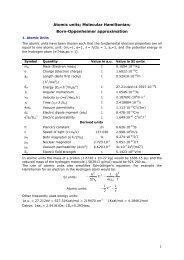
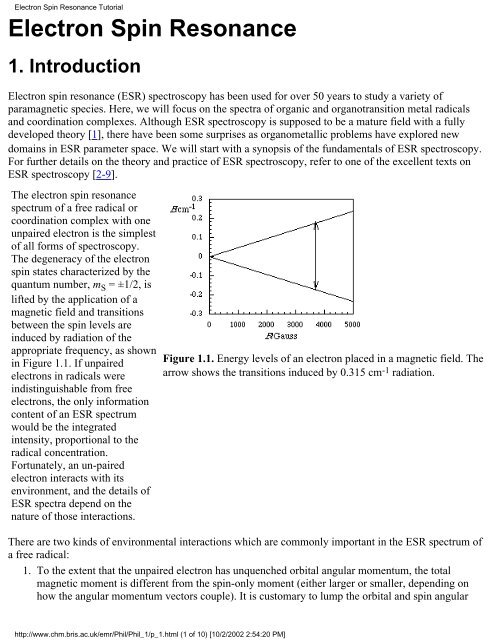
The electron spin resonance 

spectrum of a free radical or 

coordination complex with one 

unpaired electron is the simplest 

of all forms of spectroscopy. 

The degeneracy of the electron 

spin states characterized by the 

quantum number, m S = ±1/2, is 

lifted by the application of a 

magnetic field and transitions 

between the spin levels are 

induced by radiation of the 

appropriate frequency, as shown 

in Figure 1.1. If unpaired 

electrons in radicals were 

indistinguishable from free 

electrons, the only information 

content of an ESR spectrum 

would be the integrated 

intensity, proportional to the 

radical concentration. 

Fortunately, an un-paired 

electron interacts with its 

environment, and the details of 

ESR spectra depend on the 

nature of those interactions. 

Figure 1.1. Energy levels of an electron placed in a magnetic field. The 

arrow shows the transitions induced by 0.315 cm -1 radiation. 

There are two kinds of environmental interactions which are commonly important in the ESR spectrum of 

a free radical: 

1. To the extent that the unpaired electron has unquenched orbital angular momentum, the total 

magnetic moment is different from the spin-only moment (either larger or smaller, depending on 

how the angular momentum vectors couple). It is customary to lump the orbital and spin angular 

http://www.chm.bris.ac.uk/emr/Phil/Phil_1/p_1.html (1 of 10) [10/2/2002 2:54:20 PM]


2. 

momenta together in an effective spin and to treat the effect as a shift in the energy of the spin 

transition. 

The electron spin energy levels are split by interaction with nuclear magnetic moments – the nuclear 

hyperfine interaction. Each nucleus of spin I splits the electron spin levels into (2I + 1) sublevels. 

Since transitions are observed between sublevels with the same values of m I, nuclear spin splitting 

of energy levels is mirrored by splitting of the resonance line. 

2. The E.S.R. Experiment 

When an electron is placed in a magnetic field, the degeneracy of the electron spin energy levels is lifted 

as shown in Figure 1 and as described by the spin Hamiltonian: 

(2.1) 

In eq (2.1), g is called the g-value (g e = 2.00232 for a free electron), µ B is the Bohr magneton (9.274 × 10 

−28 J G −1), B is the magnetic field strength in Gauss, and S z is the z-component of the spin 

angular momentum operator (the field defines the z-direction). The electron spin energy levels are easily 

found by application of the spin Hamiltonian to the electron spin eigenfunctions corresponding to m S = 

±1/2: 

Thus 

(2.2) 

The difference in energy between the two levels, 

DE = E + - E - = gµ BB 

corresponds to the energy of a photon required to cause a transition: 

hn = gµ BB (2.3) 

or in wave numbers: 

(2.4) 

where g e µ B /hc = 0.9348 ×10 -4 cm -1G -1. Since the g-values of organic and organometallic free radicals are 

usually in the range 1.8 - 2.2, the free electron value is a good starting point for describing the experiment. 

Magnetic fields of up to ca. 15000 G are easily obtained with an iron-core electromagnet; thus we could 

use radiation with up to 1.4 cm -1 (n < 42 GHz or l > 0.71 cm). Radiation with this kind of wavelength is 

in the microwave region. Microwaves are normally handled using waveguides designed to transmit over a 



relatively narrow frequency range. Waveguides look like rectangular cross-section pipes with dimensions 

on the order of the wavelength to be transmitted. As a practical matter, waveguides can't be too big or too 

small – 1 cm is a bit small and 10 cm a bit large; the most common choice, called X-band microwaves, has 

l in the range 3.0 - 3.3 cm (n ˜ 9 - 10 GHz); in the middle of X-band, the free electron resonance is found 

at 3390 G. 

Although X-band is by far the most common, ESR spectrometers are available commercially in several 

frequency ranges: 

Designation n/GHz l/cm B (electron)/Tesla 

S 3.0 10.0 0.107 

X 9.5 3.15 0.339 

K 23 1.30 0.82 

Q 35 0.86 1.25 

W 95 0.315 3.3 

Sensitivity 

As for any quantum mechanical system interacting with electromagnetic radiation, a photon can induce 

either absorption or emission. The experiment detects net absorption, i.e., the difference between the 

number of photons absorbed and the number emitted. Since absorption is proportional to the number of 

spins in the lower level and emission is proportional to the number of spins in the upper level, net 

absorption is proportional to the difference: 

Net Absorptionµ N– – N + 

The ratio of populations at equilibrium is given by the Boltzmann distribution: 

(2.5) 

For ordinary temperatures and ordinary magnetic fields, the exponent is very small and the exponential 

can be accurately approximated by the expansion, e –x ˜ 1 – x. Thus: 

Since N – ˜N + ˜ N/2, the population difference can be written 



(2.6) 

This expression tells us that ESR sensitivity (net absorption) increases with decreasing temperature and 

with increasing magnetic field strength. Since field is proportional to microwave frequency, in principle 

sensitivity should be greater for K-band or Q-band or W-band spectrometers than for X-band. However, 

since the K-, Q- or W-band waveguides are smaller, samples are also necessarily smaller, usually more 

than canceling the advantage of a more favorable Boltzmann factor. 

Under ideal conditions, a commercial X-band spectrometer can detect the order of 10 12 spins (10 –12 

moles) at room temperature. By ideal conditions, we mean a single line, on the order of 0.1 G wide; 

sensitivity goes down roughly as the reciprocal square of the linewidth. When the resonance is split into 

two or more hyperfine lines, sensitivity goes down still further. Nonetheless, ESR is a remarkably 

sensitive technique, especially compared with NMR. 

Saturation 

Because the two spin levels are so nearly equally populated, magnetic resonance suffers from a problem 

not encountered in higher energy forms of spectroscopy: An intense radiation field will tend to equalize 

the populations, leading to a decrease in net absorption; this effect is called "saturation". A spin system 

returns to thermal equilibrium via energy transfer to the surroundings, a rate process called spin-lattice 

relaxation, with a characteristic time, T 1, the spin-lattice relaxation time (rate constant = 1/T 1). Systems 

with a long T 1i.e., spin systems weakly coupled to the surroundings) will be easily saturated; those with 

shorter T 1will be more difficult to saturate. Since spin-orbit coupling provides an important energy transfer 

mechanism, we usually find that odd-electron species with light atoms (e.g., organic radicals) have long 

T 1's, those with heavier atoms (e.g., organotransition metal radicals) have shorter T 1's. The effect of 

saturation is considered in more detail in Appendix I, where the phenomenological Bloch equations are 

introduced. 

Nuclear Hyperfine Interaction 

When one or more magnetic nuclei interact with the unpaired electron, we have another perturbation of the 

electron energy, i.e., another term in the spin Hamiltonian: 

(2.7) 

(Strictly speaking we should include the nuclear Zeeman interaction, gBI z. However, in most cases the 

energy contributions are negligible on the ESR energy scale, and, since observed transitions are between 

levels with the same values of m I, the nuclear Zeeman energies cancel in computing ESR transition 

energies.) Expanding the dot product and substituting the raising and lowering operators for S x, S y, I x, and 

I y ( ), we have 



(2.8) 

Suppose that the nuclear spin is 1/2; operating on the spin functions, we get: 

The Hamiltonian matrix thus is 

If the hyperfine coupling is sufficiently small, A


field, there are two levels corresponding to a spin singlet (E = –3A/4) and a triplet (E = +A/4). 

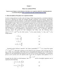
At high field, the four levels 

divide into two higher levels (m S 

= +1/2) and two lower levels 

(m S= –1/2) and approach the 

first-order results, eq (2.10) (the 

first-order solution is called the 

high-field approximation). In 

order to conserve angular 

momentum, transitions among 

these levels can involve only one 

spin flip; in other words, the 

selection rules are Dm S = ±1, 

Dm I = 0 (ESR transitions) or 

Dm S = 0, Dm I = ±1 (NMR 

transitions); the latter involves 

much lower energy photons, and, 

in practice, only the Dm S = ±1 

transitions are observed. In 

Figure 2.1, these transitions are 

marked for a photon energy of 

0.315 cm –1. 

Figure 2.1. Energy levels for an electron 

interacting with a spin 1/2 nucleus, g = 2.00, A 

= 0.10 cm –1. The arrows show the transitions 

induced by 0.315 cm–1 radiation. 

3. Operation of an ESR Spectrometer 

Although many spectrometer 

designs have been produced over 

the years, the vast majority of 

laboratory instruments are based 

on the simplified block diagram 

shown in Figure 3.1. 

Microwaves are generated by the 

Klystron tube and the power 

level adjusted with the 

Attenuator. The Circulator 

behaves like a traffic circle: 

microwaves entering from the 

Klystron are routed toward the 

Cavity where the sample is 

mounted. 

http://www.chm.bris.ac.uk/emr/Phil/Phil_1/p_1.html (6 of 10) [10/2/2002 2:54:20 PM] 

Figure 3.1. Block diagram of an ESR spectrometer.


Microwaves reflected back from the cavity (less when power is being absorbed) are routed to 

the diode detector, and any power reflected from the diode is absorbed completely by the Load. 

The diode is mounted along the E-vector of the plane-polarized microwaves and thus produces a 

current proportional to the microwave power reflected from the cavity. Thus, in principle, the 

absorption of microwaves by the sample could be detected by noting a decrease in current in the 

microammeter. In practice, of course, such a d.c. measurement would be far too noisy to be 

useful. 

The solution to the signal-to-noise ratio 

problem is to introduce small amplitude field 

modulation. An oscillating magnetic field is 

super-imposed on the d.c. field by means of 

small coils, usually built into the cavity walls. 

When the field is in the vicinity of a resonance 

line, it is swept back and forth through part of 

the line, leading to an a.c. component in the 

diode current. This a.c. component is amplified 

using a frequency selective amplifier, thus 

eliminating a great deal of noise. The 

modulation amplitude is normally less than the 

line width. Thus the detected a.c. signal is 

proportional to the change in sample 

absorption. As shown in Figure 3.2, this 

amounts to detection of the first derivative of 

the absorption curve 

Figure 3.3. First-derivative curves show better 

apparent resolution than do absorption curves. 


Figure 3.2.Small-amplitude field modulation 

converts absorption curve to first-derivative. 

It takes a little practice to get used to looking at 

first-derivative spectra, but there is a distinct 

advantage: first-derivative spectra have much 

better apparent resolution than do absorption 

spectra. Indeed, second-derivative spectra are 

even better resolved (though the 

signal-to-noise ratio decreases on further 

differentiation).


The microwave-generating klystron tube 

requires a bit of explanation. A schematic 

drawing of the klystron is shown in Figure 3.3. 

There are three electrodes: a heated cathode 

from which electrons are emitted, an anode to 

collect the electrons, and a highly negative 

reflector electrode which sends those electrons 

which pass through a hole in the anode back to 

the anode. 

Figure 3.3. Schematic drawing of a 

microwave-generating klystron tube. 

The motion of the charged electrons from the hole in the anode to the reflector and back to the 

anode generates a oscillating electric field and thus electromagnetic radiation. The transit time 

from the hole to the reflector and back again corresponds to the period of oscillation (1/n). Thus 

the microwave frequency can be tuned (over a small range) by adjusting the physical distance 

between the anode and the reflector or by adjusting the reflector voltage. In practice, both 

methods are used: the metal tube is distorted mechanically to adjust the distance (a coarse 

frequency adjustment) and the reflector voltage is adjusted as a fine control. 

Figure 3.4. Microwave cavity. 

Figure 3.5. Klystron mode and cavity dip. 

The sample is mounted in the microwave 

cavity, shown in Figure 3.4. The cavity is a 

rectangular metal box, exactly one 

wavelength in length. An X-band cavity has 

dimensions of about 1 ×2 ×3 cm. The 

electric and magnetic fields of the standing 

wave are shown in the figure. Note that the 

sample is mounted in the electric field nodal 

plane, but at a maximum in the magnetic 

field. 

Since the cavity length is not adjustable but 

it must be exactly one wavelength, the 

spectrometer must be tuned such that the 

klystron frequency is equal to the cavity 

resonant frequency. The tune-up procedure 

usually includes observing the klystron 

power mode. That is, the klystron reflector 

voltage is swept, and the diode current is 

plotted on an oscilloscope or other device. 

When the klystron frequency is close to the 

cavity resonant frequency, much less power is reflected from the cavity to the diode, resulting in 

a dip in the power mode as shown in Figure 3.5. The "cavity dip" is centered on the power mode 

using the coarse mechanical frequency adjustment with the reflector voltage used to fine tune 

the frequency. 



4. Isotropic ESR Spectra 

An isotropic ESR spectrum& #150; the spectrum of a freely tumbling radical in liquid solution& #150; 

can contain several kinds of chemically useful information: 

1. The hyperfine coupling pattern provides information on the numbers and kinds of magnetic nuclei 

with which the unpaired electron interacts. 

2. The spacing of the lines and the center of gravity of the spectrum yield the hyperfine coupling 

constants, and g-value, , which are related to the way in which the unpaired electron spin 

density is distributed in the molecule. 

3. The integrated intensity of the spectrum is proportional to the concentration of radicals in the 

sample. 

4. The spectral linewidths are related to the rate of the rotational motions which average anisotropies 

in the g- and hyperfine matrices (see §5) and to the rates of fluxional processes which average 

nuclear positions in a radical. 

5. The saturation behavior of a spectrum – the variation of integrated intensity with microwave power 

– is related to the spin-lattice relaxation time, a measure of the rate of energy transfer between the 

electron spin and its surroundings. 

The degree to which these kinds of information have been exploited varies widely. Although 

experimentalists often make qualitative observations relating "strong" or "weak" spectra to chemical 

circumstances, quantitative applications of integrated intensities are rare in ESR studies. This could be a 

useful analytical approach in some cases. The interested reader is referred to Wertz and Bolton [5], who 

discuss the technique, point out the variables which must be controlled, and suggest intensity standards. 

Largely because spin-orbit coupling results in spin state admixture, electronic spin-lattice relaxation times 

are normally short for species containing heavy atoms such as transition metals. This has two 

consequences. Short relaxation times mean that saturation problems, which plague ESR spectroscopists 

studying organic radicals and NMR spectroscopists in general, are largely absent in organometallic ESR 

studies. Thus spectra ordinarily can be recorded at full microwave power with salutary consequences for 

sensitivity. On the other hand, relaxation times are most easily determined by measuring spectral intensity 

as a function of microwave power in the saturation region. If relaxation times are short, very high power is 

required, out of the range of operation of most spectrometers. 

Line Positions in Isotropic Spectra 

ESR spectra of radicals in liquid solution are usually interpreted in terms of a spin Hamiltonian 

(4.1) 

where µ B is the Bohr magneton. The first term of eq (4.1) represents the Zeeman interaction of the 

effective electron spin, , and the applied magnetic field, , and the second represents the nuclear 

hyperfine interaction of and the nuclear spins, . The spectral information is contained in the 

parameters, , the effective gyromagnetic ratio org-value, and , the electron-nuclear hyperfine 



coupling constant for nucleus i. Using spin functions based on the quantum numbers m S and m i, eq (4.1) 

can be used to compute energy levels. Equating energy differences for the allowed transitions (Dm S = ±1, 

Dm i = 0) with the microwave photon energy, 

E(m S = 1/2) − E(m S = −1/2) = hn (4.2) 

the resonant magnetic field can be predicted. To first-order in perturbation theory, the resonant field is 

(4.3) 

where B 0 = hn/µ B represents the center of the spectrum and = / µ B is the hyperfine 

coupling constant in field units. 

The coupling constant in eq(4.1) has energy units, but the energies are very small so that frequency (MHz) 

or wave number (10 -4 cm -1) units are more commonly used. Even more often, however, isotropic coupling 

constants are given in units of magnetic field strength, usually gauss, though SI purists sometimes use 

millitesla (1 mT = 10 G). Conversions from units of gauss to frequency or wave number units involves the 

g-value 

/MHz = 2.8025 (/g e) /G (4.4a) 

/10 –4 cm –1 = 0.93480 (/g e) /G (4.4b) 

Note that coupling constants in 10 –4 cm –1 are comparable in magnitude to those expressed in gauss. 

Although the units used for isotropic hyperfine coupling constants is largely a matter of taste, the 

components of an anisotropic hyperfine coupling matrix (see §5) should be given in frequency or wave 

number units unless the g-matrix is virtually isotropic 

(continued) 


Part 2 of Phil Reiger's chapter on Electron Spin Resonance. 

Hyperfine Coupling Patterns 

Nuclear hyperfine coupling results in a multi-line ESR spectrum, analogous to the spin-spin coupling 

multiplets of NMR spectra. ESR spectra are simpler to understand than NMR spectra in that 

second-order effects normally do not alter the intensities of components; on the other hand, ESR 

multiplets can be much more complex when the electron interacts with several high-spin nuclei, and, as 

we will see below, there can be considerable variation in linewidth within a spectrum. 

When several magnetically equivalent nuclei are present in a radical, some of the multiplet lines are 

degenerate, resulting in variations in component intensity. Equivalent spin 1/2 nuclei such as 1 H, 19 F, or 

31 P result in multiplets with intensities given by binomial coefficients (1:1 for two nuclei, 1:2:1 for two, 

1:3:3:1 for three, 1:4:6:4:1 for four, etc.). One of the first aromatic organic radical anions studied by ESR 

spectroscopy was the naphthalene anion [11], the spectrum of which is shown in Figure 4.1. The 

spectrum consists of 25 lines, a quintet of quintets as expected for hyperfine coupling to two sets of four 

equivalent protons. 

Figure 4.1. ESR spectrum of the naphthalene anion radical (From Reference 11); stick spectra at the 

bottom show the 1:4:6:4:1 quintets corresponding to coupling to the two sets of four equivalent protons. 

The naphthalene anion radical spectrum provided a number of surprises. It was a surprise at the time that 

such an odd-electron species would be stable, but in the absence of air or other oxidants, [C 10 H 8 ] – is 

stable virtually indefinitely. A second surprise was the appearance of hyperfine coupling to the protons. 

The odd electron was presumed (correctly) to occupy a p * MO with the protons in the nodal plane. The 

mechanism of coupling (discussed below) requires "contact" between the unpaired electron and the 

proton, an apparent impossibility. A third surprise was the ratio of the magnitudes of the two couplings, 

5.01 G/1.79 G = 2.80. This ratio is in surprising agreement with the ratio of charge densities predicted for 

the lowest unoccupied MO (LUMO) at the a and b positions by simple Hückel MO theory, 2.62. This 

result led to Hückel MO theory being used extensively in the semi-quantitative interpretation of ESR 

spectra of aromatic radicals. 



Just as in NMR, a multiplet pattern gives an important clue to the identity of a radical. For example, the 

series of radicals derived from the nucleophilic displacement of Co(CO) – 

4 from [(RCCR')Co2 (CO) – 

6 by 

CO, phosphines, or phosphites was identified in large part from the resulting hyperfine patterns [12]. 

Depending on the nucleophile, spectra were observed which showed coupling to 0, 1, 2, or 3 31P nuclei, 

but always to a single 59Co nucleus. The parameters and aCo were found to depend slightly on the 

substituents on the acetylene moiety, suggesting that the acetylene was retained in the radical, but 

otherwise the parameters were nearly constant over the series, suggesting a single family of radicals. The 

appearance of 0 - 3 phosphorus couplings suggested three additional ligands, either CO or a phosphine or 

phosphite. Taken together, this information identified the radicals as (RCCR')CoL3 , where L = CO, PR3 , 

or P(OR) 3 . Figure 4.2(a) shows the experimental first-derivative spectrum of (Ph2C2 )Co(CO) 2P(OMe) 3 , 

1, and Figure 4.2(c) shows a first-order "stick spectrum" showing the line positions ( = 2.061, aCo = 

45.2 G, aP = 176.2 G). Hyperfine coupling to 59Co (I = 7/2) and 31P (I = 1/2) nuclei results in an octet of 

doublets. The spectrum is somewhat complicated by the obvious variation in linewidth, but the 

assignments are quite straightforward. 

Figure 4.2. (a) Isotropic ESR spectrum of (Ph 2 C 2 )Co(CO) 2 P(OMe) 3 (1) in THF solution at 260 K (from 

reference 12); (b) Second-order "stick spectrum"; (c) First-order "stick spectrum". 

Nuclei with I > 1/2 give less familiar multiplet intensity ratios. Thus, for example, three equivalent 59 Co 

nuclei (I = 7/2) give (to first order) 22 lines with intensity ratios 1:3:6:10:15:21:28:36:42:46:48:48:46..., 

as shown in Figure 4.3(a). The experimental spectrum of [PhCCo 3 (CO) 9 ] – , 2 [13], which shows this 

coupling pattern, is given in Figure 4.3(c). 

Spin Hamiltonian Parameters from Spectra 

Once a hyperfine pattern has been recognized, the line position information can be summarized by the 

spin Hamiltonian parameters, and . These parameters can be extracted from spectra by a linear 

least-squares fit of experimental line positions to eq (4.3). However, for high-spin nuclei and/or large 

couplings, one soon finds that the lines are not evenly spaced as predicted by eq (4.3) and second-order 

corrections must be made. Solving the spin Hamiltonian, eq (4.1), to second order in perturbation theory, 

eq (4.3) becomes 



(4.5) 

The magnitude of the second-order corrections is often quite significant. For example, Figure 4.2(b) 

shows a stick spectrum computed to second-order for 1. Notice that all lines are shifted to low field, 

relative to the first-order spectrum, but, as expected from eq (4.5), the shift depends on m Co . Failure to 

account for the second-order terms in an analysis results in a significant error in both the g-value and in 

the hyperfine coupling constants. For large I i and a, well-resolved spectra may warrant inclusion of thirdor 

higher-order corrections. Since the third-order corrections involve cross terms among coupling 

constants, in principle they permit determination of the relative signs of the coupling constants. However, 

in the example of Figure 4.2, the third-order corrections amount to ca. 0.1 - 0.2 G, too small to be 

significant given the resolution of the experimental spectrum. When coupling constants are really large, it 

is better to fit line positions to the exact energy levels given by the Breit-Rabi equation [10,14]. 

Figure 4.3. "Stick spectrum" showing hyperfine pattern for coupling to three equivalent 59 Co nuclei (I = 

7/2) computed to (a) first-order and (b) second-order in perturbation theory; (c) Isotropic ESR spectrum 

of [PhCCo 3 (CO)9] – in THF solution at 40°C (from reference 13). 

Second Order Splittings 



Equation (4.5) describes line positions correctly for spectra with hyperfine coupling to two or more 

nuclei provided that the nuclei are not magnetically equivalent. When two or more nuclei are completely 

equivalent, i.e., both instantaneously equivalent and equivalent over a time average, then the nuclear 

spins should be described in terms of the total nuclear spin quantum numbers J and m J rather than the 

individual I i and m i . In this "coupled representation", the degeneracies of some multiplet lines are lifted 

when second-order shifts are included. This can lead to extra lines and/or asymmetric line shapes. The 

effect was first observed in the spectrum of the methyl radical, CH 3 . The three equivalent protons lead to 

a nondegenerate nuclear spin state with J = 3/2 (m = ±3/2, ±1/2) and a two-fold degenerate state with J = 

1/2 (m = ±1/2). Thus six hyperfine lines are observed under conditions of high resolution, as shown in 

Figure 4.4 

Figure 4.4. ESR spectrum of the methyl radical, CH 3 (from reference 15; note discontinuities in magnetic 

field axis). 

Another example is the spectrum of a tricobaltcarbon radical anion, where the three equivalent spin 7/2 

59 Co nuclei should be described in terms of 11 J-states with J ranging from 21/2 to 1/2. The mJ = 17/2 

feature, for example, has three components with J = 21/2, 19/2, and 17/2, degeneracies of 1, 2, and 3, and 

second-order shifts of 97 2 /4B, 55 2 /4B, and 17 2 /4B, respectively. The shifts are too small to 

be resolved, but they lead to an asymmetric absorption line envelope with apparent broadening on the 

low-field side, as shown in Figure 4.3(a) and as is observed in the experimental spectrum of 2, shown in 

Figure 4.3(c) [13]. 

Interpretation of Isotropic Parameters 

When ESR spectra were obtained for the benzene anion radical, [C6H6 ] – , and the methyl radical, CH3 , 

the proton hyperfine coupling constants were found to be 3.75 G and 23.0 G, respectively. Since each 

carbon atom of the benzene anion carries an electron spin density of 1/6, the two results suggest that the 

proton coupling to an electron in a p* orbital is proportional to the spin density on the adjacent carbon 

atom, 

= QCHH rCp (4.6) 



where the parameter Q CHH = 23.0 G, based on CH 3 , 22.5 G, based on [C 6 H 6 ] – , or 23.7 G, based on a 

valence-bond theoretical calculation [16]. An isotropic hyperfine coupling to H can only arise through 

the so-called Fermi contact interaction of the unpaired electron with the H nucleus, and this is symmetry 

forbidden for organic p-radicals where the H nuclei lie in the plane of symmetry. The interaction arises in 

a slightly more complicated way: "spin polarization". As shown in Figure 4.5, the C 2p z orbital has zero 

probability at the H nucleus, but there is significant overlap of the C 2p z and H 1s orbitals, Suppose the H 

1s orbital is part of a s-bonding MO and the C 2p z part of the singly-occupied p* MO. In the overlap 

region of these two MO's, there is a tendency for the unpaired spin in the SOMO to polarize the pair of 

electrons in bonding MO such that the spins in the overlap region are parallel, necessarily leaving an 

oppositely oriented spin near the H nucleus. 

Figure 4.5. Schematic representation of spin 

polarization of a C-H s-orbital by electron spin 

in a p* orbital. Note that the polarization effect 

is far from complete; only a tiny fraction of the 

electron density near the H nucleus is excess 

spin-down. 

It is sometimes assumed that there is a relation analogous to eq (4.6) for metal or ligand hyperfine 

couplings in spectra of organometallic radicals. Such an assumption is usually unwarranted. An isotropic 

hyperfine coupling has three contributions: 

1. Fermi contact interaction between the nuclear spin and electron spin density in the valence-shell 

s-orbital 

2. Fermi contact interaction between the nuclear spin and spin density in inner-shell s-orbitals arising 

from spin polarization by unpaired electron density in valence-shell p- or d-orbitals 

3. a contribution from spin-orbit coupling. 

The first contribution is positive (for a positive nuclear magnetic moment), the second is normally 

negative, and the third may be of either sign. Because direct involvement of hydrogen 1s character in the 

SOMO of an organic p-radical is symmetry-forbidden and spin-orbit coupling is negligible in 

carbon-based radicals, proton couplings in such radicals result solely from spin polarization and thus are 

proportional to the polarizing spin density. All three contributions are usually significant for 

organometallic radicals. Although there are a few cases where polarization constants, analogous to 

QCHH , have been estimated [17], they are of use only in a more complete analysis based on the results of 

a solid state ESR study. 

As we will see below, g-matrices are often difficult to interpret reliably. The interpretation of isotropic 

g-values is even more dangerous. Thus isotropic ESR spectra should be used to characterize a radical by 

means of the hyperfine coupling pattern, to study its dynamical properties through linewidth effects, or to 

measure its concentration by integration of the spectrum and comparison with an appropriate standard, 

but considerable caution should be exercised in interpreting the g-value or nuclear hyperfine coupling 

constants. 



Linewidths in Isotropic Spectra 

Incomplete Averaging of Anisotropies. Isotropic ESR spectra usually show variations in linewidth 

from one hyperfine component to another (see, for example, Figures 4.2(a) and 4.3). The widths can 

often be expressed as a power series in the nuclear spin quantum numbers, 

(4.7) 

Much of the width arises from incomplete averaging of anisotropies in the g- and hyperfine matrices (see 

§5), and the parameters of eq (4.7) depend on Dg = g || – g ^ ,D Ai = A i,|| – A i,^ and t R , the rotational 

correlation time: 

a – a 0 µ (Dg)2t R (4.8a) 

b i µ Dg DA i t R (4.8b) 

g i µ (DAi)2t R (4.8c) 

Since these terms are proportional to t R , they increase with decreasing temperature. There are several 

linewidth contributions, included in a 0 , which do not depend on m i . These include the spin-rotation 

interaction which increases with 1/t R and thus with increasing temperature. These and other linewidth 

effects have been studied in some detail and are discussed elsewhere [17 - 19]. 

If the g- and hyperfine anisotropies are known from analysis of a solid-state spectrum, the linewidth 

parameters b i and g i can be used to compute the rotational correlation time,t R , a useful measure of 

freedom of motion. Linewidths in ESR spectra of nitroxide spin labels, for example, have been used to 

probe the motional freedom of biological macromolecules [20]. Since t R is related to the molecular 

hydrodynamic volume, V h , and the solution viscosity, h, by : 

t R = hV h /k B T (4.9) 

ESR linewidths can provide a measure of the effective size of a paramagnetic molecule or ion, useful 

information when there is a suspicion that a radical has polymerized. Thus, for example, vanadium(IV) 

shows an eight-line ESR spectrum in basic aqueous solution, suggesting a monomeric unit, 

[VO(OH) 3 (H2O) 2 ] – [21], although previous work on the system had indicated polymers such as V3O 2– 

7 

or V4O 2– 

9 . Comparison of values of tR from the basic solution linewidths with those obtained from 

spectra of acidic solutions containing VO(H2O) 2+ 

5 showed that the hydrodynamic volume of the aquo 

cation is actually about twice that of the basic solution species, effectively ruling out the presence of 

ESR-active polymers in solution [22]. 

Rates of Fluxionality from Linewidths. ESR linewidths are also sensitive to processes which modulate 

the g-value or hyperfine coupling constants or limit the lifetime of the electron spin state. The effects are 

closely analogous to those observed in NMR spectra of dynamical systems. However, since ESR 

linewidths are typically on the order of 0.1-10 G (0.3-30 MHz), rate processes which give observable 

increases in linewidths must be fast. Bimolecular processes which contribute to ESR linewidths have 

mostly been nearly diffusion-controlled, e.g., intermolecular electron exchange between naphthalene and 



its anion radical [23] and reversible axial ligation of square planar copper(II) complexes [24]. 

The effect of rate processes on linewidths can be understood quantitatively in terms of the modified 

Bloch equations ([25], see also Appendix 3), or, more accurately, in terms of density matrix [26] or 

relaxation matrix [18, 27] formalisms. If a rate process modulates a line position through an amplitude 

DB (Dw in angular frequency units) by fluctuating between two states, each with lifetime t, a single line 

is observed with an excess width proportional to (Dw)2t when t–1 >> Dw – the fast exchange limit. As 

the lifetime increases, the line broadens to indetectability and then re-emerges as two broad lines. These 

shift apart and sharpen until, in the slow exchange limit (t-1


1:2:1 triplet of octets; the spectrum is complicated by a large linewidth dependence on mCo , but as 

demonstrated in Figures 4.7(b) and 4.7(c), the central lines of the triplets are much broader than the outer 

lines. This radical has a distorted tetrahedral structure with the semi-occupied molecular orbital (SOMO) 

largely cobalt 3d 2 

z in character [29]. Thus the ligand sites can be described as axial or equatorial relative 

to the unique z-axis. Several isomers are possible, but the 31P couplings distinguish between the isomer 

with an axial phosphite (ax,eq) and those with either CO or the acetylene axial and both phosphites 

equatorial (eq,eq). The rate of interconversion between eq,eq and ax,eq isomers was estimated from the 

relative widths of the mP = ±1 and 0 lines, given the isotropic coupling constants for the various 31P nuclei (which were determined from the frozen solution spectrum [29]). The average rate was found to 

be approximately 2 ×1010 s –1 (Ea = 17 kJ mol –1 ) at 298 K. 

Figure 3.7. ESR spectrum of (Ph 2 C 2 )Co(CO)[P(OMe) 3 ] 2 (a) Experimental spectrum of THF solution at 

290 K; (b and c) Computer-simulated spectra including (b) the m Co and m P linewidth dependence, and (c) 

the m Co linewidth dependence only. 

5. Anisotropic ESR Spectra 



The anisotropies which lead to line broadening in isotropic ESR spectra influence solid-state spectra 

more directly. Accordingly a more complex spin Hamiltonian is required to interpret such spectra 

In eq (5.1), g and A i are 3 × 3 matrices representing the anisotropic Zeeman and nuclear hyperfine 

interactions. In general, a coordinate system can be found (the g-matrix principal axes) in which g is 

diagonal. If g and A i are diagonal in the same coordinate system, we say that their principal axes are 

coincident. 

In species with two or more unpaired electrons, a fine structure term must be added to the spin 

Hamiltonian to represent electron spin-spin interactions. We will confine our attention here to radicals 

with one unpaired electron (S = 1/2) but will address the S > 1/2 problem in Section 6. 

Nuclear quadrupole interactions introduce line shifts and forbidden transitions in spectra of radicals with 

nuclei having I > 1/2. In practice, quadrupolar effects are observable only in very well-resolved spectra 

or in spectra of radicals with nuclei having small magnetic moments and large quadrupole moments. The 

most extreme case of a small magnetic moment to quadrupole moment ratio is that of 191Ir/ 193Ir, and 

spectra of [Ir(CN) 6 ] 3– [30], [Ir(CN) 5Cl] 4– and [Ir(CN) 4Cl2 ] 4– [31], and 

[Ir2 (CO) 2 (PPh3 ) 2 (m-RNNNR) 2 ] + , R = p-tolyl [32], show easily recognizable quadrupolar effects. Other 

nuclei for which quadrupolar effects might be expected include 151Eu/ 153Eu, 155Gd/ 157Gd, 175Lu, 181Ta, 189Os, and 197Au. When quadrupolar effects are important, it is usually necessary to take account of the 

nuclear Zeeman interaction as well. The nuclear quadrupole and nuclear Zeeman interactions add two 

more terms to the spin Hamiltonian. Since these terms considerably complicate an already complex 

situation, we will confine our attention here to nuclei for which quadrupolar effects can be neglected. 

When a radical is oriented such that the magnetic field direction is located by the polar and azimuthal 

angles,q and f, relative to the g-matrix principal axes, the resonant field is given, to first order in 

perturbation theory, by [33] 

(5.1) 

(5.2) where (5.3) 

g 2 = g x 2 sin2qcos2f + gy 2 sin2qsin2f+ gz 2 cos2q (5.4) 

A i 2 = Aiz 2 Six 2 + Aiy 2 Siy 2 + Aiz 2 Siz 2 (5.5) 

S ik = [g x sin q cos f l ixk + g y sin q cos f l iyk + g z cos q l izk ]/g (5.6) 

and the lijkare direction cosines indicating the orientation of the kth principal axis of the ith hyperfine 

matrix relative to the jth g-matrix principal axis. When the matrix principal axes are coincident, only one 

of the lijk of eq (4.6) will be nonzero. When the hyperfine matrix components are large, second-order 

terms [33] must be added to eq (5.2); these result in down-field shifts, proportional to m 2 

i . 

Solid-State ESR Spectra 



So long as they are dilute (to avoid line broadening from intermolecular spin exchange), radicals can be 

studied in the solid state as solutes in single crystals, powders, glasses or frozen solutions. Radicals can 

be produced in situ by UV- or g-irradiation of a suitable precursor in a crystalline or glassy matrix. While 

many organometallic radicals have been studied in this way [34], it is often easier to obtain solid state 

ESR spectra by freezing the liquid solution in which the radical is formed. A variety of techniques then 

can be used to generate radicals, e.g., chemical reactions, electrochemical reduction or oxidation, or 

photochemical methods. Furthermore, the radical is studied under conditions more closely approximating 

those in which its reaction chemistry is known. 

Spectra of Dilute Single Crystals. Spectra of radicals in a dilute single crystal are obtained for a variety 

of orientations, usually with the field perpendicular to one of the crystal axes. Spectra usually can be 

analyzed as if they were isotropic to obtain an effective g-value and hyperfine coupling constants. Since 

the g- and hyperfine matrix principal axes are not necessarily the same as the crystal axes, the matrices, 

written in the crystal axis system usually will have off-diagonal elements. Thus, for example, if spectra 

are obtained for a variety of orientations in the crystal xy-plane, the effective g-value is 

gf2 = (gxx cos f + gyx sin f)2 + (gxy cos f + gyy sin f)2 + (gxz cos f + gyz sin f)2 (5.7) 

or gf2 = K1+ K2 cos 2f + K3 sin 2f (5.8) 

where K1 = (gxx2 + gyy2 + gxz2 + gyz2 + 2 gxy2)/2 (5.9a) 

K2 = (gxx2 - gyy2 + gxz2 - gyz2)/2 (5.9b) 

K3 = gxy(gxx + gyy) + gxzgyz (5.9c) 

A sinusoidal plot of gf2 vs f can be analyzed to determine K1, K2, and K3. Exploration of another crystal 

plane gives another set of K's which depend on other combinations of the gij; eventually enough data are 

obtained to determine the six independent gij (g is a symmetric matrix so that gij = gji). The g2-matrix 

then is diagonalized to obtain the principal values and the transformation matrix, elements of which are 

the direction cosines of the g-matrix principal axes relative to the crystal axes. An analogous treatment of 

the effective hyperfine coupling constants leads to the principal values of the A2-matrix and the 

orientation of its principal axes in the crystal coordinate system. 

Analysis of Powder Spectra. Since ESR spectra are normally recorded as the first derivative of 

absorption vs. field, observable features in the spectrum of a powder correspond to molecular orientations 

for which the derivative is large in magnitude or changes in sign. For any spin Hamiltonian, there will be 

minimum and maximum resonant fields at which the absorption changes rapidly from zero, leading to a 

large value of the derivative and features which resemble positive-going and negative-going absorption 

lines. Peaks in the absorption envelope correspond to derivative sign changes and lead to features 

resembling isotropic derivative lines. The interpretation of a powder spectrum thus depends on the 

connection of the positions of these features to the g- and hyperfine matrix components. 

Early treatments of powder patterns attempted to deal with the spatial distribution of resonant fields by 

analytical mathematics [35]. This approach led to some valuable insights but the algebra is much too 

complex when nonaxial hyperfine matrices are involved. Consider the simplest case: a single resonance 

line without hyperfine structure. The resonant field is given by eq (5.3). Features in the first derivative 

spectrum correspond to discontinuities or turning points in the absorption spectrum which arise when 

B/q or B/f are zero, 



(5.10a) 

or (5.10b) 

These equations have three solutions: (i) q = 0; (ii) q= 90°, f = 0; and (iii) q = f = 90°. Since q and f are in 

the g-matrix axis system, observable features are expected for those fields corresponding to orientations 

along the principal axes of the g-matrix. This being the case, the principal values of the g-matrix are 

obtained from a straightforward application of eq (5.3). 

Powder spectra with hyperfine structure often can be interpreted similarly with spectral features 

identified with orientation of the magnetic field along one of the g- and hyperfine matrix principal axes. 

However, this simple situation often breaks down. Using a first-order theory and one hyperfine coupling, 

Ovchinnikov and Konstantinov [36] have shown that eqs (5.10) may have up to six solutions 

corresponding to observable spectral features. Three of these correspond to orientation of B along 

principal axes, but the "extra lines" correspond to less obvious orientations. Even more extra lines may 

creep in when the spin Hamiltonian is treated to second order or when there is more than one hyperfine 

coupling. The problem is illustrated by the resonant field vs. cos q and f surface shown in Figure 5.1, 

corresponding to the mCu = –3/2 "line" in the spectrum of Cu(acac)2 (g = 2.0527, 2.0570, 2.2514; ACu = 

27.0, 19.5, 193.4 ¥ 10–4 cm–1) [36]. The minimum resonant field, B = 3290.7 G, corresponds to B along 

the z-axis (cos q = ±1). With B along the x-axis (cos q = 0, f = 0°), the surface shows a saddle point at 

3344.3 G, and with B along the y-axis (cos q = 0, f = 90°), there is a local minimum at 3325.5 G. In 

addition, another saddle point occurs in the yz-plane at B = 3371.2 G (cos q = ±0.482, f = 90°); the only 

maximum is in the xz-plane at B = 3379.0 G (cos q = ± 0.459, , f = 0°). Thus five features are expected 

and indeed are shown in the computer-simulated spectrum of Cu(acac)2 shown in Figure 5.2. The two 

high-field features correspond to off-axis field orientations and thus are "extra lines". The situation is 

more complex when the g- and hyperfine matrix principal axes are noncoincident (see below); in this 

case, none of the features need correspond to orientation of B along a principal axis direction. 

Figure 5.1. 

Res-onant field as 

a function of cos 

q and f for the 

mCu = -3/2 "line" 

of the frozen 

solution spectrum 

of Cu(acac)2; ESR 

parameters from 

reference 36. 



Since the analytical approach is so complicated, powder patterns have usually been analyzed by 

comparing the experimental spectrum with a spectrum, computer-simulated using estimates of the g- and 

hyperfine matrix components. Parameters are then adjusted and another simulation computed until the fit 

is satisfactory (or the experimentalist loses patience with the problem). The most straightforward 

computer simulation method [37] involves computation of the resonant magnetic field using eq (5.2) for 

ca. 105 values of cos q and f for each set of nuclear spin quantum numbers. The field is then divided into 

equal increments and the number of times the resonant field falls between Bi and Bi+1 is plotted vs. B to 

give an approximation to the unbroadened absorption spectrum. The absorption spectrum is then 

broadened by numerical convolution with a line shape function and differentiated to give the desired 

simulation. Although the "cut and try" approach to spectrum analysis works reasonably well when there 

are small numbers of parameters, analysis of a complex spectrum is exceedingly tedious. 

DeGray and Rieger [38] have developed a computer algorithm to locate powder pattern features in 

spectra, given estimates of the spin Hamiltonian parameters. The method employs a search of the 

resonant field surface in cos q, f space for maxima, minima, and saddle points. Since the search 

procedure requires computation of B for ~100 orientation, the method is much faster than a complete 



Figure 5.2. Computer-simulated first-derivative ESR powder spectrum of Cu(acac)2. (a) Features 

corresponding to mCu = –3/2; (b) Complete spectrum. 

simulation. The predicted locations of spectral features then are compared with the experimental values 

and the parameters refined using a nonlinear least-squares method. Using this method, relatively complex 

powder patterns can be analyzed, provided that the spectrum is sufficiently well resolved that enough 

features can be located and identified to determine the parameters. Even with least-squares fitting, 

however, comparison of the experimental spectrum with a computer simulation is required to check the 

assignments of spectral features. 

Interpretation of the g-Matrix 

The g-value of a free electron is a scalar, ge = 2.00232. In a radical species, g becomes a matrix because 

of the admixture of orbital angular momentum into S through spin-orbit coupling. The components of the 

g-matrix thus differ from ge to the extent that p-, d- or f-orbital character has been incorporated and 

differ from one another, depending on which p- , d- or f-orbitals are involved. 

In general, the components of the g-matrix are given by 

(5.11) 

where the indices i and j refer to molecular coordinate axes (x, y, z), k sums over atoms with unpaired 

electron density, and m sums over filled and empty molecular orbitals with energy Em (E0 is the energy 

of the SOMO); zk is the spin-orbit coupling constant for atom k, and lki is the i-component orbital 

angular momentum operator for atom k. The integrals are easily computed if the MO's are written 

as linear combination of real p or d atomic orbitals. The results of operation by li on these functions is 

shown in Table 5.1. Thus, for example, = i and = – i. 

Notice that dz2 is unique among the d-orbitals in that lz does not couple it to any other orbital. Thus if 



the major metal contribution to the SOMO is dz2, gz will be close to the free electron value. 

Accordingly, when one g-matrix component is found close to the free electron value, it is often taken as 

evidence for a dz2-based SOMO; such reasoning should be applied with caution, however, since 

cancellation of negative and positive terms in eq (5.11) could have the same effect. 

Spin-orbit coupling to empty MO's (E0 – Em < 0) gives a negative contribution to gij whereas coupling 

to filled MO's has the opposite effect. Thus ESR spectra of d1 vanadium(IV) complexes generally have 

g-values less than ge (admixture of empty MO's) whereas d9 copper(II) complexes have g-values greater 

than ge (admixture of filled MO's). 

Since the g-matrix has only three principal values and there are almost always many potentially 

interacting molecular orbitals, there is rarely sufficient information to interpret a g-matrix with complete 

confidence. When a well resolved and reliably assigned optical spectrum is available, the energy 

differences, E0 – Em, are known and can be used in eq (5.11). Extended Hückel MO calculations can be 

useful (but don't trust EHMO energies!), but one is most commonly reduced to arguments designed to 

show that the observed g-matrix is consistent with the interpretation placed on the hyperfine matrix. 

Table 5.1. Angular momentum operations on the real p and d orbitals. 

lx ly lz 

0 –i i 

i 0 –i 

–i i 0 

–i –i 2i 

i –i –2i 

i + i i –i 

–i i – i i 

– i i 0 

Interpretation of the Hyperfine Matrix 

Electron-nuclear hyperfine coupling arises mainly through two mechanisms: 

1. The Fermi contact interaction between the nuclear spin and s-electron spin density; this 

contribution is isotropic and has been discussed above. 

2. The electron spin-nuclear spin magnetic dipolar interaction; this contribution is almost entirely 

anisotropic, i.e., neglecting spin-orbit coupling, the average dipolar contribution to the hyperfine 

coupling is zero. 



The general form of the dipolar contribution to the hyperfine term of the Hamiltonian is 

(5.12) 

where ge and gN are the electron and nuclear g-values, mB and mN are the Bohr and nuclear magnetons, 

and the matrix element is evaluated by integration over the spatial coordinates, leaving the spins as 

operators. Equation (5.12) can then be written 

(5.13) 

where Ad is the dipolar contribution to the hyperfine matrix, 

A = ·AÒ E + Ad (5.14) 

(E is the unit matrix). In evaluating the matrix element of eq (5.12), the integration over the angular 

variables is quite straightforward. The integral over r, however, requires a good atomic orbital 

wavefunction. Ordinarily, the integral is combined with the constants as a parameter 

(5.15) 

P has been computed using Hartree-Fock atomic orbital wavefunctions and can be found in several 

published tabulations [39-42]. Because of the dependence of P, dipolar coupling of a nuclear spin 

with electron spin density on another atom is usually negligible. 

If an atom contributes px, py, and pz atomic orbitals to the SOMO 

(5.16) 

the total p-orbital spin density is (in the Hückel approximation, i.e., neglecting overlap): 

rp = cx2 + cy2 + cz2 (5.17) 

and the dipolar contribution to the hyperfine matrix can be written 

(Ad)ij = (2/5)Plij (5.18) 

where the lij are lxx = 2cx2 – cy2 – cz2 (5.19a) 

lyy = –cx2 + 2cy2 – cz2 (5.19b) 

lzz = –cx2 – cy2 + 2cz2 (5.19c) 

lij = –3cicj (i j) (5.19d) 

The dipolar hyperfine matrix for p-orbitals can always be written 



(5.20) 

The p-orbital axis corresponds to the positive principal value of the matrix. When the p-orbitals are 

written as hybrids, the orbital shape is unchanged, but the principal axes of the hyperfine matrix, which 

reflect the spatial orientation of the hybrid p-orbital, differ from those in which the SOMO was 

formulated. Thus, for example, a p-hybrid with cx = cz (cy = 0) corresponds to a p-orbital with the major 

axis in the xz-plane and halfway between the x- and z-axes (Euler angle b = 45°). 

Similarly, if an atom contributes d atomic orbitals to the SOMO, 

(5.21) 

the total d-orbital spin density is (in the Hückel approximation): 

(5.22) 

and the dipolar contribution to the hyperfine matrix is [43] 

(Ad)ij = (2/7)Plij (5.23) 

where P is given by eq (5.15) and the lij are: 

(5.24d) 

(5.24c) 

(5.24e) 

(5.24f) 

(5.24a) 

(5.24b) 

The dipolar contribution to the hyperfine matrix for a pure d-orbital is 

(5.25) 

where the positive sign applies for dz2 and the lower sign to the other four orbitals. Hybrid combinations 

of dyz, dxz, and dxy or dx2–y2 and dxy give a d-orbital of the same shape and the same dipolar matrix, 



though the principal axes in general are different from the axes in which the SOMO was formulated. 

Other hybrid orbitals are generally of different shape, reflected by different principal values of the 

dipolar matrix, usually with different principal axes. 

Spin-orbit coupling perturbs these results, adding terms to the diagonal matrix components on the order 

of P(gi – ge). These can be neglected only when the g-matrix anisotropy is small. Calculation of the 

spin-orbit coupling corrections is fairly straightforward for mononuclear complexes where the SOMO is 

composed mainly of d-orbitals from a single metal [6,44,45]. In radicals with two or more transition 

metals, the spin-orbit coupling calculation is seriously nontrivial. A major part of the problem is that the 

solution must be gauge-invariant, that is, it must not depend on the choice of coordinate system. This 

problem was addressed in the context of spin-orbit coupling corrections to the g-matrix [46], with eq 

(5.11) as the result, but it has received only cursory examination with regard to spin-orbit contributions to 

hyperfine matrices [47]. Fortunately, polynuclear radicals containing first-row transition metals generally 

have g-matrix components sufficiently close to ge that the problem can be ignored. For organometallic 

radicals with second- and third-row transition metals, the problem is urgent; it is to be hoped that some 

theoretician will deem the problem worthy of attention. 

The AO composition of the SOMO can often be deduced from the dipolar hyperfine matrix, particularly 

when the radical has enough symmetry to restrict possible hybridization. Thus an axial hyperfine matrix 

can usually be interpreted in terms of coupling to a single p- or d-orbital. A departure from axial 

symmetry may be due to spin-orbit coupling effects, if (for example) A||= Az and Ax - Ay ª P(gx – gy). If 

the departure from axial symmetry is larger, it is usually caused by d-orbital hybridization. The 

procedure is best illustrated by example. 

Example–A low-spin Manganese(II) Complex 

The spectrum of the low-spin manganese(II) complex, [Mn(dppe)2(CO)(CNBu)]2+, 5 (dppe = 

Ph2PCH2CH2PPh2) [48], in a CH2Cl2/THF glass is shown in Figure 5.3a. The spin Hamiltonian 

parameters, obtained from a least-squares fit of the field positions of the spectral features [49], are given 

in Table 2, and a computer simulation based on those parameters is shown in Figure 5.3b. 

Table 2. ESR Parameters for [Mn(dppe)2(CO)(CNBu)]2+. 

g AMn/10-4 cm-1 AP/10-4 cm-1 

2.107 30.2 27.2 

2.051 20.6 25.3 

1.998 146.9 26.4 

5 has approximate C2v symmetry, although the actual symmetry is reduced to C2 or Cs, depending on 

the conformation of the ethylene bridges of the dppe ligands. Since 5 has a nominal d5 configuration, the 

SOMO is expected to be one of the "t2g" orbitals of an idealized octahedral complex–dxz (b1), dyz (b2), 

or dx2-y2 (a1), where the representations refer to C2v. The energies of the dxz and dyz orbitals are 

expected to be lowered by back-donation into the ¹* orbitals of the CO and CNBu ligands so that the 



SOMO is most likely based on dx2-y2, possibly with some symmetry-allowed dz2 admixture, 

Figure 5.3. (a) ESR 

spectrum of 5 in a 

CH2Cl2/THF glass 

(49); (b) Computer 

simula-tion using the 

para-meters of Table 2. 

(5.26) 

Although the isotropic spectrum of 5 was not sufficiently resolved to unambiguously determine , 

other closely related species give isotropic couplings on the order of 60-70 G [49]; if we assume an 

isotropic coupling in this range, all three matrix components must have the same sign. If the isotropic 

hyperfine coupling is negative, as expected if it arises mostly through polarization of inner-shell s 

orbitals, we have = –65.9 ¥ 10–4 cm–1. Assuming that the SOMO is mostly dx2–y2, (b >> a) and 

including the appropriate spin-orbit coupling corrections, we have [29,45] 

(5.27) 

With Dgz = –0.004, (Dgx + Dgy) = 0.154, and P = 207.6 ¥ 10–4 cm–1 [40], we get (a2 – b2) = –0.655. 



The departure from axial symmetry is due to spin-orbit coupling and/or dx2-y2/dz2 hybridization, 

(5.28) 

Substituting the parameters, we have ab = ±0.058. (The upper sign applies if the components are listed in 

the order x, y, z in Table 2, the lower sign if the order is y, x, z) Finally, we get b2 = 0.660, a2 = 0.005. 

The dz2 component is not really significant, given the accuracy of the data and the theory, i.e., most of 

the departure from axial symmetry can be explained by the spin-orbit coupling correction. 

Using eq (5.11), the g-matrix components are found to be 

(5.29a) 

(5.29b) 

(5.29c) 

If we assume coupling with single pure dyz, dxz, and dxy orbitals, we have DEyz = 16z, DExz = 19z, 

DExy = –1100z, qualitatively consistent with the expected MO energy level scheme. 

Example: Some Cobalt(0) Radical Anions 

ESR spectra of [CpCo(1,3-COD)]–, 6, in frozen THF solution and [CpCo(1,5-COD)]–, 7, in frozen DMF 

were reported by Geiger and coworkers [50] and are reproduced in Figures 5.4a and 5.5a. These spectra 

have been reinterpreted to give the parameters shown in Table 3; computer-simulated spectra based on 

these parameters are shown in Figures 5.4b and 5.5b. Also shown in the table are the ESR parameters for 

[(C5Ph5)Co(CO)2]–, 8 [44]. 

Table 3. ESR parameters for Cobalt(0) Radical Anions. 

Radical Anion gx gy gz Axa Aya Aza 

[CpCo(1,5-COD)]– 2.171 2.027 1.985 (-)158.6 (-)36.7 (-)45.8 

[CpCo(1,3-COD)]– 2.151 2.027 1.997 (-)139.2 (-)36.4 (-)38.2 

[(C5Ph5)Co(CO)2]–b 2.018 2.041 1.995 (-)157.9 (-)16.8 (-)44.1 



a Units of 10–4 cm–1. b From reference 44. 

The hyperfine matrix components must 

have identical signs in order that the 

average values match the observed 

isotropic couplings; we assume the 

signs are negative since the isotropic 

couplings almost certainly arise from 

polarization of inner shell s orbitals (see 

below). 

The SOMO in these radicals is expected 

from extended Hückel MO calculations 

[50,51] to be primarily cobalt 3dyz in 

character. In the Cs symmetry of the 

radicals, dyz belongs to the a" 

representation and d-hybridization is 

possible only with dxy. Assuming that 

such hybridization is negligible, the 

g-matrix components are given by [44] 

(5.30a) 

(5.30b) 

(5.30c) 

The dipolar contribution to the 

hyperfine matrix is given by eq (5.20), 

but spin-orbit coupling contributions 

are significant. These often can be ex- 

Figure 5.4. ESR spectrum of 

[CpCo(1,3-COD)]–; (a) experimental 

spectrum in frozen THF solution (from 

reference 50); (b) computer-simulation, 

based on the parameters of Table 3. 

pressed in terms of the g-matrix components (as in the Mn(II) example discussed above), but here 

spin-orbit coupling with the four other d-orbitals contributes somewhat differently to the g-matrix and to 

the hyperfine matrix. The simplest way of expressing the hyperfine matrix is in terms of the isotropic 

coupling, the x-component, and the departure from axial symmetry, 



(5.31c) 

(5.31a) 

(5.31b) 

With the assumed signs of the hyperfine components of Table 3, eq (5.31b) can be used unambiguously 

to compute a2 = rd with the results shown in Table 4. 

Since 3dyz/4s admixture is symmetry-forbidden for these radicals, the Fermi contact contribution to the 

isotropic coupling must be entirely from spin polarization, 

As = Qdrd (5.32) 

Thus we can obtain an independent estimate of the d-electron spin density from the values of As, taking 

Qd = –131 ¥ 10–4 cm–1, estimated from the isotropic cobalt coupling in [PhCCo3(CO)9]–. The results 

are shown in the last column of Table 4. The spin densities estimated from the isotropic couplings are 

consistently about 10% higher than those from the dipolar coupling matrix, suggesting a systematic error 

in one of the parameters, but a reliable ordering of the spin densities. 

Table 4. d-Electron spin densities in cobalt(0) radical anions. 

Radical Anion rd Asa As/Qd 

[CpCo(1,5-COD)]- 0.681 -97.0 0.740 

[CpCo(1,3-COD)]- 0.591 -87.2 0.666 

[(C5Ph5)Co(CO)2]-b 0.540 -77.4 0.591 

a in units of 10–4 cm–1. 

The g-matrix presents an interesting problem in these cases. EHMO calculations [50,51] suggest that the 

SOMO is the highest-energy MO which is primarily cobalt 3d in character. At lower energy is an orbital 

with dxz character and still lower, but grouped at about the same energy, are MO's with dx2–y2, dxy, and 

dz2 contributions. Equations (5.30) then would suggest that Dgxx/4 Å Dgyy < Dgzz. With the 

assignments of Table 4, the first relationship is approximately correct for 6 and 7, but very poor for 8. 

The second relationship is not found for any of the anions. Reversing the y and z assignments makes the 

agreement worse. In discussing this problem for 8 [44], we postulated admixture of some cobalt 4py 

character in the SOMO, 



(5.33) 

Figure 5.5. ESR spectrum of [CpCo(1,5-COD)]-; (a) experimental spectrum in frozen DMF solution 

(from reference 50); (b) computer-simulation, based on the parameters of Table 3 

which would result in additional contributions to gxx and gzz, 

gxx(p) = 2zpb2/DEz and gzz(p) = 2zpb2/DEx (5.34) 

where zp is the cobalt 4p spin-orbit coupling parameter (zp Å zd/3). If MO's with significant pz or px 

character lie just above the SOMO, then gxx and gzz would be less positive than expected from eqs 

(5.30), possibly even negative. gxx is indeed smaller than expected for 8 and EHMO calculations do 

indeed suggest a MO with significant pz character just above the SOMO in energy; this orbital is 

apparently substantially higher in energy in 6 and 7. A MO with significant px character, at about the 

same energy for all three anions, is implied by these results but is unsubstantiated by the reported EHMO 

calculations. 

Noncoincident Matrix Axes 

In general, the g- and nuclear hyperfine coupling matrices, g and Ai, can be written in diagonal form with 

three principal values–gx, gy, gz and Aix, Aiy, Aiz. In textbooks on ESR [2-7], it is usually assumed that 

the same set of principal axes diagonalizes all the relevant matrices. While this is sometimes true, there 

are many instances where the principal axes are noncoincident [52]. 

Symmetry Considerations. Kneubühl [53,54] has given a detailed group theoretical analysis of 

symmetry restrictions on the orientations of g- and hyperfine matrix principal axes. His results are 

summarized in Table 5. For a nucleus sharing all the molecular symmetry elements (e.g., the metal 



nucleus in a mononuclear complex), the hyperfine matrix is subject to the same restrictions as the 

g-matrix. In orthorhombic or axial symmetry, such nuclear hyperfine matrices necessarily share principal 

axes with the g-matrix. In monoclinic symmetry, one hyperfine axis is also a g-matrix axis, but the other 

two may be different. In triclinic symmetry (C1 or Ci), none of the three principal axes need be shared 

by the g-matrix and hyperfine matrix. The hyperfine matrix for a ligand atom (or for a metal in 

polynuclear complexes) is constrained only by the symmetry elements which the nucleus shares with the 

molecule. 

Table 5. Symmetry restrictions on g-matrix components. 

Symmetry 

Point Groups 

Restrictions 

on Diagonal 

Elements 

Restrictions on 

Off-Diagonal 

Elements 

Required 

Matrix 

Axes 

Triclinic C1,Ci none none none 

Monoclinic C2,Cs,C2h none gxz = gyz = 0 z 

Orthorhombic C2v,D2,D2h none gxz = gyz = gxy 

=0 

Axial Cn,Cnv,Cnh, 

Dn,Dnd,Dnh, n > 

2 

gxx = gyy gxz = gyz = gxy 

=0 

Although symmetry considerations often permit g- and hyperfine matrix principal axes to be 

noncoincident, there are relatively few cases of such noncoincidence reported in the literature. Most of 

the examples discussed by Pilbrow and Lowrey in their 1980 review [52] are cases of transition metal 

ions doped into a host lattice at sites of low symmetry. This is not to say that matrix axis noncoincidence 

is rare but that the effects have only rarely been recognized. 

Experimental Determination of Matrix Axis Orientations. We have seen that spectra of dilute single 

crystals are analyzed in a way that gives the orientations of the g- and hyperfine matrix principal axes 

relative to the crystal axes. Historically, most of the information on noncoincident matrix axes is derived 

from such studies. 

At first glance, it would appear that all orientation dependence should be lost in the spectrum of a 

randomly oriented sample and that location of the g- and hyperfine matrix principal axes would be 

impossible. While it is true that there is no way of obtaining matrix axes relative to molecular axes from 

a powder pattern, it is frequently possible to find the orientation of a set of matrix axes relative to those 

of another matrix. 

The observable effects of matrix axis noncoincidence on powder patterns range from blatantly obvious to 

negligible. In general, the effects of axis noncoincidence will be more noticeable if two (or more) 

matrices have large anisotropies which are comparable in magnitude, e.g., DgmBB Å DA. This follows 

from the fact that minimum and maximum resonant fields are determined by a competition between 


x,y,z 

x,y,z


extrema in the angle-dependent values of g and A. Consider the case of noncoincident g- and hyperfine 

matrix axes. For large values of |mI|, the field extrema will be determined largely by the extrema in the 

effective hyperfine coupling and will occur at angles close to the hyperfine matrix axes, but for small 

|mI|, the extrema will be determined by extrema in the effective g-value and will correspond to angles 

close to the g-matrix axes. The result of such a competition is that a series of features which would be 

equally spaced (to first order) acquires markedly uneven spacings. 

There are two corollaries stemming from this generalization. Since spin 1/2 nuclei give only two 

hyperfine lines, there can be no variation in spacings. Thus powder spectra cannot be analyzed to extract 

the orientations of hyperfine matrix axes for such important nuclei as 1H, 13C, 19F, 31P, 57Fe, and 

103Rh. Secondly, since the observable effects in powder spectra depend on the magnitude of the matrix 

anisotropies, the principal axes of the hyperfine matrix for a nucleus with small hyperfine coupling 

generally cannot be located from a powder spectrum, even though the relative anisotropy may be large. 

Example–Chromium Nitrosyl Complex 

A good example of the effect of g- and hyperfine matrix axis noncoincidence is the ESR spectrum of 

[CpCr(CO)2NO]–, 9, studied by Geiger and coworkers [55] and 

Figure 5.6. Computer-simulated 

(a)absorption and (b) 

first-deriva-tive spectra of 9. 

Example–Iron Pentacarbonyl Ions 

and shown in Figure 5.6. The g- and 14N 

hyperfine matrices are approximately axial 

for this radical, but the g|| axis lies close to 

the perpendicular plane of the hyperfine 

matrix. If the g|| axis was exactly in the A^ 

plane, the three negative-going g|| A^ 

features, corresponding to resonant field 

maxima, would be evenly spaced. In fact, 

the spacings are very uneven, far more so 

than can be explained by second-order 

shifts. The effect can be understood, and the 

spectrum simulated virtually exactly, by 

assuming that the g|| axis is about 15° out of 

the A^ plane. 

Two particularly interesting organometallic examples were reported by Morton, Preston and 

coworkers [56,57]. Spectra of single crystals of Cr(CO)6, doped with 13C- or 57Fe-enriched Fe(CO)5 

and g-irradiated at 77 K, showed two different radicals. One species, identified as Fe(CO)5+, showed 

coupling to 57Fe and to a unique 13C nucleus with axial hyperfine matrices sharing principal axes with 

the g-matrix [56]. Coupling was also observed to four other 13C nuclei with identical coupling matrices 

but with the major axis approximately along the g-matrix x-axis for two nuclei and along the g-matrix 



y-axis for the other two. The parameters are listed in Table 6. If the radical is square pyramidal (C4v) 

Fe(CO)5+, 10, the principal axes of the g-matrix must be the molecular axes (the C4 axis and normals to 

the reflection planes). The iron atom and the carbon of the axial CO group have the full symmetry of the 

group and so these hyperfine matrices must share principal axes with the g-matrix. The four equatorial 

carbonyl carbons, on the other hand, lie in reflection planes, but not on the C4-axis and so are 

symmetry-required to share only one principal axis with the g-matrix. In fact, the major matrix axes for 

the equatorial carbons are tilted slightly in the -z direction from the ideal locations along the ±x and ±y 

axes. The g-matrix suggests that the metal contribution is dz2 and the iron hyperfine matrix then can be 

used to estimate about 55% iron 3d and 34% axial carbon 2pz spin density. The spin density on the 

equatorial carbons then is mostly negative and due to spin polarization. 

Table 6. ESR Parameters for Fe(CO)5+ and Fe(CO)5–.a 

Fe(CO)5+: g|| = 2.001 A||Fe = (+)9.4 A||C1 = 

(+)19.6 

A||C2-C5 = 

(+)6.4 

g^ = 2.081 A^Fe = (-)6.2 A^C1 = (-)17.6 A^C2-C5 = 

(+)8.6 

Fe(CO)5–: g1 = 1.989 A1Fe = (+)6.7 A1C1 = 

(+)87.4 

g2 = 2.003 A2Fe = (-)4.5 A2C1 = 

(+)70.7 

g3 = 2.010 A3Fe = (-)3.2 A3C1 = 

(+)65.7 

a Coupling constants in units of 10–4 cm–1. Data from references 56 and 57. 

The other species observed in irradiated Fe(CO)5-doped crystals of Cr(CO)6 also showed coupling to 

57Fe, to a unique 13C, and to four other carbons. However, in this case g, AFe, and AC1 have only one 

matrix axis in common (that corresponding to the third component of each matrix listed in Table 6). The 

other 57Fe hyperfine axes are rotated by about 27° and those of the 13C hyperfine matrix by about 48° 

relative to the g-matrix axes. Insufficient data were accumulated to determine the complete hyperfine 

matrices for the other four carbons, but the components are considerably smaller (4 - 15 ¥ 10–4 cm–1). 

The hyperfine matrices suggest about 38% iron 3dz2, 18% carbon 2p, and 6% carbon 2s spin densities. 

Using detailed arguments regarding the orientation of the g-matrix axes relative to the crystal axes, the 



authors conclude that the carbon 2p axis is oriented at about 106° relative to the Fe-C bond axis and that 

the Fe-C-O bond angle is about 119°. 

The most striking feature of these results is the orientation of the unique 13C hyperfine matrix axes, 

relative to those of the 57Fe hyperfine axes. This orientation led Fairhurst, et al.[57], to assign the 

spectrum to Fe(CO)5–, 11, and to describe the species as a substituted acyl radical. However, these 

authors did not discuss the orientation of the g-matrix axes. The y-axis, normal to the reflection plane, is 

common to all three matrices. The x- and z- axes of the g-matrix, on the other hand are oriented about 27° 

away from the corresponding 57Fe hyperfine matrix axes. Since the iron d-orbital contribution to the 

SOMO appears to be nearly pure dz2, the 57Fe hyperfine matrix major axis must correspond to the local 

z-axis, assumed to be essentially the Fe-C bond. Thus we must ask: Why are the g-matrix axes different? 

The SOMO can be written 

(5.35) 

where a = 0.62, bx = -0.41, and bz = 0.12. Spin-orbit coupling will mix the SOMO with MO's having 

iron dyz or dxz character, but dyz is involved in the p orbitals of the C=O group, 

(5.36) 

Assuming that there is only one p orbital close enough in energy to couple significantly, eq (5.11) gives 

the g-matrix components: 

Dgzz = 0 (5.37c) 

(5.37b) 

(5.37d) 

(5.37a) 

The g-matrix can be diagonalized by rotation about the y-axis by the angle b, 

(5.38) 

With b = 27°, this expression gives cyz/cy Å 0.5, a reasonable result. 

This may be a rather general effect; if the unpaired electron in a radical is delocalized asymmetrically, 

and other MO's are similarly delocalized, the g-matrix will have off-diagonal elements which may be 

large enough to shift the principal axes away from the molecular coordinate system. 



Example–Another low-spin Manganese(II) Complex 

The low-spin manganese(II) complex, [Mn(dppe)2(CO)(CNBu)]2+, 5, gave us a textbook example of a 

well-behaved ESR spectrum characterized by coincident g- and hyperfine matrix principal axes. The 

nearly identical complex, [Mn(dppm)2(CO)(CN)]+, 12+, provides us with a good example of 

non-coincident principal axes. The frozen solution spectrum, shown in Figure 5.7, shows that 

Figure 5.7. ESR spectrum of 12+ in 

CH2Cl2/C2H4Cl2 at 90 K; from 

reference (49). 

interaction would result. In order to 

avoid this interaction, two things 

happen: (1) incorporation of dxz 

char-acter tilts the lobes up and down, 

away from the C atoms. At the same 

time, the x-ray structure of the Mn(II) 

cation shows (Figure 5.8) that the CH2 

groups tilt down and up, further 

decreasing the anti-bonding interaction. 

With only one electron in the SOMO, 

the anti-bonding interaction is strong 

enough to produce this distortion. With 

two electrons, the neutral parent Mn(I) 

complex would be expected to be even 

more distorted, and an x-ray structure 

shows that the up and down 

displacements of the CH2 groups is 

the "parallel" features are not evenly 

spaced. The spectrum can be 

understood if the z-axes of the g- and 

A-matrices are displaced by b = 19.6°. 

This, of course, tells us that the 

molecule does not have C2v 

symmetry, and that, unlike the dppe 

analog, dx2-y2 is not the only Mn 

contribution to the SOMO. One way 

of interpreting the results is that the 

Mn contribution to the SOMO 

incorporates a small amount of dxz 

character. The consequence of this 

hybridization would be to tilt the "x" 

lobes of dx2-y2 up and down, i.e., 

rotation about the y-axis. The reason 

for this hybridization is not difficult to 

discover. If the CH2 groups of the 

dppm ligands were coplanar with Mn, 

the "x" lobes of the dx2-y2 SOMO 

would be directed toward the carbon 

atoms and an anti-bonding 

Figure 5.8. X-ray structure of 12+, 

showing methylene groups tilted up and 

down to avoid anti-bonding interaction 

with dx2-y2 SOMO. 



approximately doubled. 

Example–Chromium(I) Piano-Stool Complex 

Ordinarily, there is no way of extracting the orientation of the principal axes of the g-matrix from a 

powder or frozen solution ESR spectrum. However, there are exceptional circumstances in which nature 

is kind to the experimentalist! 

Spectra of the low-spin d5 Cr(I) 

complex, [(C5Ph5)Cr(CO)2PMe3] 13 

(58), are shown at 125 and 200 K in 

Figure 5.9 The low-temperature 

spectrum shows three sets of doublets, 

corresponding to the three 

g-components (2.104, 2.013, 1.994), 

each a doublet due to hyperfine 

coupling to 31P. At 200 K, above the 

freezing point of toluene, the spectrum 

still appears as a "powder pattern", but 

the "perpendicular" features are nearly 

averaged and the "parallel" features 

have shifted upfield (g|| = 2.090, g^ = 

2.012). The exceptionally bulky C5Ph5 

ligand apparently moves very slowly at 

200 K but on the ESR time scale the 

Cr(CO)2PMe3 moiety rotates quickly, 

producing a spectrum averaged about 

the Cr-C5 axis. With this interpretation, 

we can assign this axis as the principal 

axis for g|| measured at 200 K and, 

assuming that the g|| axis differs from 

the gz axis by 

the angle b and that gz and gx are averaged according to 

2g||2 = gz2 + gx2 + (gz2 + gx2) cos22b 

Substitution of the g-components gives b = 15° 

Figure 5.9. Spectra of 13 in toluene at 

125 and 200 K; from reference (58). 

The symmetry of the complex is at most Cs, requiring one of the g-matrix principal axes to be normal to 

the plane of symmetry, assumed to be xz. ¹-back-bonding to the CO ligands is expected to lead to a 

hybrid SOMO. If, as suggested by extended Hückel MO calculations, the SOMO and first HOMO are of 

a' symmetry, and the second HOMO of a" symmetry: 



the g-matrix components can be computed: 

Rotation about the y-axis by b diagonalizes the matrix, and we find 

The single experimental observable, b, is hardly enough to evaluate the LCAO coefficients for the 

SOMO and second HOMO, but we can compare the results of an extended Hückel MO calculation. 

(Since zCo and E0 – E2 cancel in the calculation of tan 2b, the EHMO calculation could come close). 

The results are: a1 = 0.538, a2 = 0.216, a3 = –0.194, c1 = 0.582, c2 = –0.061, b = 14.8°. If we were to 

substitute these LCAO coefficients, together with the EHMO energy difference, into the expressions for 

gxx, gyy, gzz, and gxz, the results would be in very poor agreement with experiment; the moral here is 

that EHMO calculations, lacking charge self-consistency, usually have large errors in the energies, but 

the MO wavefunctions are often fairly accurate. 

Example–[(RCCR')Co2(CO)6]- and [SFeCo2(CO)9]- 

Noncoincident matrix axis effects are seen in the frozen solution spectra of [(RCCR')Co2(CO)6]–, 14 

[59], and [SFeCo2(CO)9]–, 15 [60], but the effects are rather more subtle than those discussed above. 

In these cases, the g-matrix is nearly isotropic, but the principal axes of the two 59Co hyperfine matrices 

are noncoincident. The largest hyperfine matrix component (ay = 66.0 G in the case of 15) results in 15 

features, evenly spaced (apart from small second-order shifts). Another series of features, less widely 

spaced, shows some variation in spacing and, in a few cases, resolution into components. This behavior 

can be understood as follows: Suppose that the hyperfine matrix y-axes are coincident and consider 

molecular orientations with the magnetic field in the xz-plane. To first order, the resonant field then is 

B = B0 - m1a+ - m2a- (5.39) 



where B0 = hn/gmB and 

a±2 = az2cos2(q ± b) + ax2sin2(q ± b) (5.40) 

where b describes the orientation of the hyperfine matrix z-axes relative to the g-matrix z-axis. Since g is 

nearly isotropic, the extrema in B are determined mostly by the hyperfine term. When m1 = m2, a+ and 

a- are equally weighted and the extrema occur at q = 0 or 90°, but when m1 m2, the extrema correspond 

to other angles. Consider, for example, the five components of the m1+ m2 = +3 feature. With |az| = 53.6 

G, |ax| = 15.5 G, b = 18°, the hyperfine contributions to the field extrema and the corresponding values of 

q are given in Table 7. In the experimental spectrum of 15, two resolved field maximum features were 

seen, corresponding to the first two and the last three of the above components. Since the resolution is 

sensitive to the noncoincidence, it was possible to fit the experimental spectrum to obtain b quite 

accurately. 

Table 7. Splitting of M = 3 features in [SFeCo2(CO)9]– Spectrum. 

(m1, m2) qmin (B-B0)min/G qmax (B-B0)max/G 

+7/2,-1/2 -20° 37.0 +67° 166.1 

-1/2,+7/2 +20° 37.0 -67° 166.1 

+5/2,+1/2 -15° 55.3 +78° 156.9 

+1/2,+5/2 +15° 55.3 -78° 156.9 

+3/2,+3/2 0° 66.5 90° 153.6 

It is relatively easy to understand the significance of the noncoincident matrix axes in these cases. For 14, 

the C2v molecular symmetry permits a specific prediction of the possible matrix axis orientations. The 

g-matrix principal axes must be coincident with the molecular symmetry axes. The two cobalt nuclei are 

located in a reflection plane (which we label xz) so that symmetry requires the y-axis to be a principal 

axis for all three matrices. The other two axes may be rotated, relative to the molecular x- and z-axes, by 

±b. (Since the two nuclei are symmetrically equivalent, the rotations must be equal and opposite.) 

Since the magnitudes and probable signs of the cobalt hyperfine matrices suggest a SOMO 

predominantly dz2 in character, the major axes of the hyperfine matrices approximate the local z-axes at 

the cobalt atoms and the angular displacement indicates a bent Co-Co anti-bonding interaction, as 

shown in structure 16, where the C-C or Fe-S bond axis (the molecular y-axis) is perpendicular to the 

plane of the page. Comparison with the crystal structure of neutral (Ph2C2)Co2(CO)6 [61] shows that 

these local axes are roughly in the direction of the axial carbonyl ligands (the Co-CO bond is tilted 28° 

away from the Co-Co vector). Thus it seems reasonable to say that the local axes on a metal are 

determined primarily by the more strongly interacting ligands and that bonds to other atoms can be 

described as bent. 

Example–(o-xylylene)-Mn(dmpe) 2 



As part of a study of Mn(II) dialkyls, Wilkinson, Hursthouse, and coworkers [62] reported the ESR 

spectrum of the approximately octahedral (o-xylylene)Mn(dmpe)2, 17, Figure 5.10a (dmpe = 

Me2PCH2CH2PMe2). The spectrum was interpreted assuming coincident g- and hyperfine matrix axes, 

but a simulation based on the reported parameters gave a very poor fit to the published spectrum. On 

closer examination, it was realized that this is a rather 

extreme example of a spectrum 

influenced by noncoincident g- and 

hyperfine matrix principal axes. The 

clue evident in the spectrum is the 

large gap between the mMn = –1/2 

and +1/2 "parallel" features, 

suggesting one or more extra 

features. Figure 5.11 shows a set of 

simulated spectra for a hypothetical 

low-spin Mn(II) species; all seven 

spectra correspond to the same gand 

hyperfine matrices, but the angle 

b, between the g- and hyperfine 

matrix z-axes, varies from 0 to 90°. 

As shown in Figure 5.11, it is 

possible to obtain spectra with more 

than six resolved "parallel" features. 

Indeed, the spectrum is sufficiently 

sensitive to the angle that b can be 

evaluated quite precisely. The final 

parameters for 17, based on 

least-squares fitting of the positions 

of the resolved features and the 

isotropic parameters [53], are given 

in Table 8; a computer simulation 

using these parameters is shown in 

Figure 5.10b. 

Figure 5.10. (a) ESR spectrum of 

(o-xylylene)Mn(dmpe)2 in frozen toluene 

solution (from reference 53); (b) Computer 

simulation of spectrum using parameters of 

Table 8. 

Table 8. ESR Parameters for (o-xylylene)Mn(dmpe)2, 17.a 

g AMn AP 

2.110 27 24.5 

2.035 27 24.5 



2.000 125 24.5 

a Hyperfine matrix components in units of 10-4 cm-1; b = 41°. 

Figure 5.11. 

Computer-simulated 

ESR spectra for a 

hypothetical low-spin 

Mn(II) radical with g = 

(2.100, 2.050, 2.000), 

AMn = (150, 25, 25) ¥ 

10–4 cm–1, for various 

values of b, the Euler 

angle between the 

g-matrix and hyperfine 

matrix z-axes. 

17 has approximate C2v symmetry, but the ethylene bridges of the dmpe ligands destroy the reflection 

planes; the x-ray structure [53] shows a small fold at the methylene groups of the o-xylylene ligand 

which destroys the C2 axis. Thus the molecule can be regarded, with increasing accuracy, as C2v, Cs, 

C2, or C1. In order to explain the matrix axis noncoincidence, the metal contribution to the SOMO must 

be a d-hybrid. Since 17 is a d5 low-spin Mn(II) species, the SOMO is expected to be dominated by one 

of the orbitals of the octahedral t2g set–dxz, dyz, or dx2-y2. This is consistent with a clue contained in 

the ESR parameters. The four 31P couplings are apparently equivalent, and all are relatively small. Thus 

no lobe of the SOMO can be directed toward a phosphorus atom, and major dxy or dz2 contributions to 

the SOMO can be ruled out. Consider the twelve binary hybrids based on these orbitals which are listed 



in Table 9. Since we know that the 

Table 9. SOMO Candidates: Binary d-Hybrids. 

Number 

Representation 

Major Minor 

Approx. 

Major Common 

Cs C2 d-AO d-AO HF Axis Axis 

1 a' a dx2-y2 dz2 z x,y,z 

2 a' - dx2-y2 dyz z x 

3 a' - dyz dx2-y2 x x 

4 a' - dyz dz2 x x 

5 a" - dxz dxy y x 

6 - a dx2-y2 dxz z y 

7 - a dxz dx2-y2 y y 

8 - a dxz dz2 y y 

9 - b dyz dxy x y 

10 - - dx2-y2 dxy z z 

11 - - dxz dyz y z 

12 - - dyz dxz x z 

hyperfine matrix major axis is not a g-matrix principal axis, we can immediately reject hybrids 1, 3, 4, 7, 

8, and 10 for which the major axis is a common axis. Hybrids 2 and 6, 5 and 9, and 11 and 12 differ only 

in the x- and y-labels and are essentially indistinguishable, so that there are only three cases to consider in 

detail. 

Hybrid 6 can be written 

(5.41) 

Straightforward application of eqs (5.24) yields a hyperfine matrix which can be diagonalized by rotation 

about the y-axis by the angle b, 

tan 2b = –2b/a (5.42) 

The g-matrix can be written in relatively simple form if we assume that the only MO's close enough in 

energy to contribute significantly are the filled MO's, primarily dxz and dyz in character. With this 



assumption, we obtain a matrix which can be diagonalized by rotation about the y-axis by b', 

(5.43) 

For reasonable values of the hybridization ratio, b/a up to about 0.5, b and b' can differ by only a few 

degrees and this kind of hybrid cannot explain the matrix axis noncoincidence. Following the same 

reasoning with x and y interchanged, exactly the same conclusions can be reached for hybrid 2. 

Hybrids 11 and 12 are 

(5.44) 

In this case, the hyperfine matrix remains axial, independent of the hybridization ratio, although the 

principal axes are rotated in the xy-plane by an angle a equal to angle b of eq (5.43). Assuming that only 

MO's with predominantly dxz, dyz, or dx2–y2 character contribute, a g-matrix is found which can be 

diagonalized by rotation in the xy-plane by the angle a', also given by eq (5.43). Thus this hybrid gives 

identical g- and hyperfine matrix principal axes for all hybridization ratios. 

Finally, hybrid 9, 

(5.45) 

gives an axial hyperfine matrix with principal axes rotated in the xz-plane by an angle b, given by eq 

(5.43). The g-matrix is somewhat more complicated, 

Diagonalization requires rotation about the y-axis by the angle b', 

where 

(5.48) 

(5.47) 


(5.46)


Since the energy differences, DEx2–y2 and DExz are expected to be comparable, the parameter Q is 

probably not far from unity. For Q = 1, eq (5.47) has a particularly simple form, tan 2b' = +2a/b so that, 

for small b/a, we expect b Å 0 and b' Å 45°, entirely consistent with experiment. The axial hyperfine 

matrix is in agreement with experiment, and the principal values of the g-matrix can also be rationalized 

with reasonable values of Q and b/a. A small rotation of dyz about the y-axis might reflect the small 

displacements of the phosphorus atoms from the idealized octahedral positions. 

An extended Hückel MO calculation on 15 supports the assumptions made in the above analysis in that 

the three "t2g" orbitals are indeed close together in energy and remain nearly nonbonding metal-based 

d-orbitals. The detailed agreement is less satisfactory: the SOMO is predicted to be primarily dx2–y2 

with a small dxz admixture (hybrid 6 of Table 9), a result which can be ruled out from our analysis of the 

ESR results. The EHMO overlap matrix based on the x-ray structure suggests that the molecule is much 

closer to C2 symmetry than to Cs. If we accept that conclusion, then dxz/dxy hybridization is less likely 

than dyz/dxy, as we tacitly assumed above. 

We considered several alternative explanations for the matrix axis noncoincidence in 15. In particular, it 

seemed possible that delocalization of spin density into the o-xylylene ligand, either through the s-bonds 

or into the p-system, might lead to significant contributions to the off-diagonal terms of the g-matrix. 

While the EHMO calculations suggest that the MO's containing dx2–y2 and dyz do have contributions 

from the carbon atoms of the o-xylylene group, the amount is far too small to rationalize rotation of the 

g-matrix axes by 41°; indeed, to explain the effect in this way would require each of several carbon 

atoms to contribute 5% or more to the MO's with dx2–y2 or dyz character, unreasonably large 

considering the poor overlap of these metal d-orbitals with the relevant carbon orbitals. 

6. Molecules with More than One Unpaired Electron 

Molecules with two or more unpaired electrons may be divided into two classes: By far the most 

common examples are molecules where the unpaired electrons are contained in a set of degenerate 

atomic or molecular orbitals with qualitatively similar spatial distributions, e.g., an octahedral Cr(III) 

(4A2g) or Ni(II) (3A2g) complex, or a triplet state molecule like O2, or the excited triplet states of 

naphthalene or benzophenone. 

A second class of molecules with 

two unpaired electrons has the two 

electrons localized, to a first 

approximation, in different parts of 

the molecule. We refer to such 

molecules as biradicals. Examples 

are the dinitroxides, and certain 

binuclear vanadium(IV) and 

copper(II) complexes. 

From the point of view of ESR spectroscopy, the distinction between molecules with one unpaired 

electron and those with more than one lies in the fact that electrons interact with one another; these 

interactions lead to additional terms in the spin Hamiltonian and additional features in the ESR spectrum. 

The most important electron-electron interaction is coulombic repulsion; with two unpaired electrons, 

repulsion leads to the singlet-triplet splitting. As we will see, this effect can be modelled by adding a 



term, , to the spin Hamiltonian, where J is called the exchange coupling constant and turns out to 

be equal to the singlet-triplet splitting. 


EMR Reference pages 

References 

1 A. Hudson, Electron Spin Resonance, 1988,11A , 55-76. 

2 P. B. Ayscough, Electron Spin Resonance in Chemistry, Methuen, London, 1967. 

3 P. W. Atkins and M. C. R. Symons, The Structure of Inorganic Radicals, Elsevier, Amsterdam, 1967. 

4 A. Abragam and B. Bleaney, Electron Paramagnetic Resonance of Transition Ions, Clarendon Press, 

Oxford, 1970. 

5 J. E. Wertz and J. E. Bolton, Electron Spin Resonance, McGraw-Hill, New York, 1972. 

6 N. M. Atherton, Electron Spin Resonance, Ellis Horwood, Chicester, 1973. 

7 W. Gordy, Theory and Applications of Electron Spin Resonance, Wiley, New York, 1980. 

8 J. R. Pilbrow, Transition Ion Electron Paramagnetic Resonance, Clarendon Press, Oxfor, 1990. 

9 F. E. Mabbs and D. Collison, Electron Paramagnetic Resonance of d Transition Metal Compounds, 

Elsevier, Amsterdam, 1992. 

10 G. Breit and I. I. Rabi, Phys. Rev. 1931, 38, 2082-2083. 

11 S. I. Weissman, J. Townsend, G. E. Paul, and G. E. Pake, J. Chem. Phys. 1953, 21, 2227. 

12 L. V. Casagrande, T. Chen, P. H. Rieger, B. H. Robinson, J. Simpson, and S. J. Visco, Inorg. Chem. 

1985, 23, 2019-2025. 

13 B. M. Peake, P. H. Rieger, B. H. Robinson, and J. Simpson, Inorg. Chem. 1979,18, 1000-1005. 

14 A. R. Boate, J. R. Morton, and K. F. Preston, J. Mag. Reson. 1976, 24, 259-268. 

15 R. W. Fessenden and R. H. Schuler, J. Chem. Phys. 1963, 39, 2147. 

16 M. Karplus and G. K. Fraenkel, J. Chem. Phys. 1961, 35, 1312. 

17 R. Wilson and D. Kivelson, J. Chem. Phys. 1966, 44, 154; P. W. Atkins and D. Kivelson, J. Chem. 

Phys. 1966, 44, 169. 

18 G. K. Fraenkel, J. Phys. Chem. 1967, 71, 139-171. 

19 W. B. Lewis and L. O. Morgan, in R. L. Carlin (Ed.), Transition Met. Chem., Vol. 4, Marcel 

Dekker, New York, 1968, pp. 33-112. 

20 B. H. Robinson and A. H. Beth, Electron Spin Resonance 1983, 8, 346-377. 

21 M. M. Iannuzzi and P. H. Rieger, Inorg. Chem. 1975,14, 2895-2899. 

22 M. M. Iannuzzi, C. P. Kubiak, and P. H. Rieger, J. Phys. Chem. 1976,80, 541-545. 

23 R. L. Ward and S. I. Weissman, J. Am. Chem. Soc. 1957,79, 2086-2090. 

24 B. J. Corden and P. H. Rieger, Inorg. Chem. 1971,10, 263-272. 

http://www.chm.bris.ac.uk/emr/Phil/References.html (1 of 3) [10/2/2002 2:55:11 PM]


25 H. S. Gutowsky, D. W. McCall, and C. P. Slichter, J. Chem. Phys. 1953, 21, 279-292. See also 

reference 6, pp 309-313. 

26 J. I. Kaplan, J. Chem. Phys. 1958, 28, 278-282; 1958, 29, 462; S. Alexander, ibid. 1962, 37, 

967-974, 974-980. See also reference 6, pp 313-323. 

27 See also reference 6, pp 323-327. 

28 N. W. Duffy, R. R. Nelson, M. G. Richmond, A. L. Rieger, P. H. Rieger, B. H. Robinson, D. R. 

Tyler, J. C. Wang and K. Yang, Inorg. Chem. 1998, 37, 4849. 

29 J. A. DeGray, Q. Meng, and P. H. Rieger, J. Chem. Soc. Faraday I 1987, 83, 3565-3573. 

30 N. V. Vugman, A. O. Caride, and J. Danon, J. Chem. Phys. 1973, 59, 4418-4422. 

31 N. V. Vugman and N. M. Pinhal, Mol. Phys. 1983,49, 1315-1319. 

J. A. DeGray, P. H. Rieger, N. G. Connelly and G. Garcia, J. Magn. Reson., 1990, , 376. 

33 P. H. Rieger, J. Magn. Reson. 1982, 50, 485-489. 

34 M. C. R. Symons, J. R. Morton, and K. F. Preston, in K. S. Suslick (Ed.), High-Energy Processes in 

Organometallic Chemistry, American Chemical Society, Washington, DC, 1987, pp. 169-190. 

35 P. C. Taylor, J. F. Baugher, and H. M. Kriz, Chem. Rev. 1975, 75, 203-240. 

36 I. V. Ovchinnikov and V. N. Konstantinov, J. Magn. Reson. 1978, 32, 179-190. 

37 P. C. Taylor and P. J. Bray, J. Magn. Reson. 1970, 2, 305-331. 

38 J. A. DeGray and P. H. Rieger, Bull. Magn. Reson. 1987, 8, 95-101. 

39 B. A. Goodman and J. B. Raynor, Adv. Inorg. Chem. Radiochem. 1971, 13, 136-362. 

40 J. R. Morton and K .F. Preston, J. Mag. Reson. 1978, 30, 577-582. 

41 A. K. Koh and D. J. Miller, Atom. Data Nucl. Data Tab. 1985, 33, 235-253. 

42 P. H. Rieger, J. Mag. Reson. 1997, 124, 140. 

43 B. M. Peake, P. H. Rieger, B. H. Robinson, and J. Simpson, J. Am. Chem. Soc. 1980, 102, 156-163. 

44 N. G. Connelly, W. E. Geiger, G. A. Lane, S. J. Raven, and P. H. Rieger, J. Am. Chem. Soc. 

1986,108, 6219-6224. 

45 B. R. McGarvey, in T. F. Yen (Ed.), Electron Spin Resonance of Metal Complexes, Plenum Press, 

New York, 1969, pp. 1-11. 

46 A. F. Stone, Proc. Roy. Soc. (London) 1963, A271, 424-434. 

47 T. Kawamura, K. Fukamachi, T. Sowa, S. Hayashide, and T. Yonezawa, J. Am. Chem. Soc. 1981, 

103, 364-369. 

48 G. A. Carriedo, V. Riera, N. G. Connelly, and S. J. Raven, J. Chem. Soc., Dalton Trans.1987, 



1769-1773. 

49 G. A. Carriedo, N. G. Connelly, E. Perez-Carreno, A. G. Orpen, A. L. Rieger, P. H. Rieger, V. 

Riera, and G. M. Rosair, J. Chem. Soc., Dalton Trans., 1993, 3103. 

50 T. A. Albright, W. E. Geiger, J. Moraczweski, and B. Tulyathan, J. Am. Chem. Soc. 1981, 103, 

4787-4794. 

51 T. A. Albright and R. Hoffmann, Chem. Ber. 1978, 111, 1578-1590. 

52 J. R. Pilbrow and M. R. Lowrey, Rep. Prog. Phys. 1980, 43, 433-495. 

53 F. K. Kneubühl, Phys. Kondens. Mat. 1963, 1, 410-447; 1965, 4, 50-62. 

54 For a summary of Kneubühl's methods, see reference 52. 

55 W. E. Geiger, P. H. Rieger, B. Tulyathan, and M. C. Rausch, J. Am. Chem. Soc. 1984, 106, 

7000-7006. 

56 T. Lionel, J. R. Morton, and K. F. Preston, J. Chem. Phys. 1982, 76, 234-239. 

57 S. A. Fairhurst, J. R. Morton, and K. F. Preston, J. Chem. Phys. 1982, 77, 5872-5875. 

58 D. J. Hammack, M. M. Dillard, M. P. Castellani, A. L. Rheingold, A. L. Rieger and P. H. 

Rieger,Organometallics, 1996, 15, 4791. 

59 B. M. Peake, P. H. Rieger, B. H. Robinson, and J. Simpson, J. Am. Chem. Soc. 1980, 102, 156. 

60 B. M. Peake, P. H. Rieger, B. H. Robinson, and J. Simpson, Inorg. Chem. 1981, 20, 2540. 

61 F. A. Cotton, J. D. Jamerson, and B. R. Stults, J. Am. Chem. Soc. 1976, 98, 1774-1779. 

62 C. G. Howard, G. S. Girolami, G. Wilkinson, M. Thornton-Pett, and M. B. Hursthouse, J. Chem. 

Soc., Dalton Trans. 1983, 2631-2637.

Electron Spin Resonance Tutorial

Create successful ePaper yourself

Delete template?

Save as template?