Transport: Non-diffusive, flux conservative initial value problems and ...
Transport: Non-diffusive, flux conservative initial value problems and ...
Transport: Non-diffusive, flux conservative initial value problems and ...

Create successful ePaper yourself
Turn your PDF publications into a flip-book with our unique Google optimized e-Paper software.
<strong>Transport</strong> equations 61<br />
concentration<br />
2.0<br />
1.5<br />
1.0<br />
0.5<br />
t=0<br />
1<br />
2<br />
3<br />
0 1 2 3 4 5 6 7 8 9 10<br />
distance<br />
Figure 5.3: Evolution of a gaussian <strong>initial</strong> condition in a constant velocity field V = 1<br />
using a FTCS scheme. A perfect scheme would have the <strong>initial</strong> gaussian just propagate<br />
at constant speed without changing its shape. The FTCS scheme however causes it to<br />
grow <strong>and</strong> eventually for high frequency noise to swamp the solution. By underst<strong>and</strong>ing<br />
the nature of the truncation error we can show that it is because the FT step has inherent<br />
negative diffusion which is always unstable.<br />
5.4.1 Hirt’s method<br />
Hirt’s method can be thought of as reverse Taylor series differencing where we start<br />
with finite difference approximation <strong>and</strong> come up with the actual continuous partial<br />
differential equation that is being solved. Given the FTCS scheme in (5.3.21) we<br />
first exp<strong>and</strong> each of the terms in a Taylor series about each grid point e.g. we can<br />
express the point c n+1<br />
j as<br />
c n+1<br />
j<br />
likewise for the spatial points c n j±1<br />
t=4<br />
= cnj + ∆t ∂c (∆t)2 ∂<br />
+<br />
∂t 2<br />
2c ∂t2 + O(∆t3cttt) (5.4.1)<br />
c n j+1 = c n j + ∆x ∂c<br />
∂x + (∆x)2∂ 2 c<br />
∂x 2 + O(∆x3 cxxx) (5.4.2)<br />
c n j−1 = c n j − ∆x ∂c<br />
∂x + (∆x)2∂ 2 c<br />
∂x 2 − O(∆x3 cxxx) (5.4.3)<br />
Substituting (5.4.1) <strong>and</strong> (5.4.2) into (5.3.21) <strong>and</strong> keeping all the terms up to second<br />
derivatives we find that we are actually solving the equation<br />
∂c ∂c<br />
+ V<br />
∂t ∂x<br />
∂<br />
= −∆t<br />
2<br />
2c ∂t2 + O(∆x2fxxx − ∆t 2 fttt) (5.4.4)<br />
To make this equation a bit more familiar looking, it is useful to transform the time<br />
derivatives into space derivatives. If we take another time derivative of the original