Transport: Non-diffusive, flux conservative initial value problems and ...
Transport: Non-diffusive, flux conservative initial value problems and ...
Transport: Non-diffusive, flux conservative initial value problems and ...

Create successful ePaper yourself
Turn your PDF publications into a flip-book with our unique Google optimized e-Paper software.
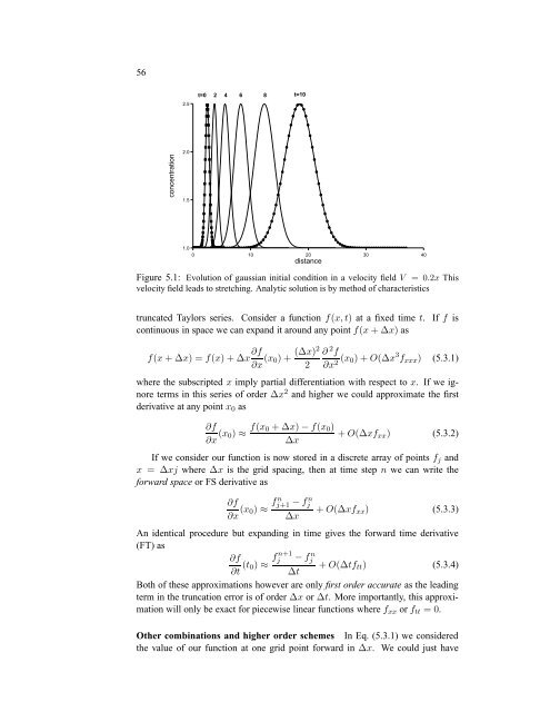
56<br />
concentration<br />
2.5<br />
2.0<br />
1.5<br />
1.0<br />
t=0 2 4 6 8 t=10<br />
0 10 20 30 40<br />
distance<br />
Figure 5.1: Evolution of gaussian <strong>initial</strong> condition in a velocity field V = 0.2x This<br />
velocity field leads to stretching. Analytic solution is by method of characteristics<br />
truncated Taylors series. Consider a function f(x,t) at a fixed time t. If f is<br />
continuous in space we can exp<strong>and</strong> it around any point f(x + ∆x) as<br />
f(x + ∆x) = f(x) + ∆x ∂f<br />
∂x (x0) + (∆x)2 ∂<br />
2<br />
2f ∂x2 (x0) + O(∆x 3 fxxx) (5.3.1)<br />
where the subscripted x imply partial differentiation with respect to x. If we ignore<br />
terms in this series of order ∆x 2 <strong>and</strong> higher we could approximate the first<br />
derivative at any point x0 as<br />
∂f<br />
∂x (x0) ≈ f(x0 + ∆x) − f(x0)<br />
+ O(∆xfxx) (5.3.2)<br />
∆x<br />
If we consider our function is now stored in a discrete array of points fj <strong>and</strong><br />
x = ∆xj where ∆x is the grid spacing, then at time step n we can write the<br />
forward space or FS derivative as<br />
∂f<br />
∂x (x0) ≈ fn j+1 − fn j<br />
∆x<br />
+ O(∆xfxx) (5.3.3)<br />
An identical procedure but exp<strong>and</strong>ing in time gives the forward time derivative<br />
(FT) as<br />
∂f<br />
∂t (t0) ≈ fn+1 j − fn j<br />
+ O(∆tftt) (5.3.4)<br />
∆t<br />
Both of these approximations however are only first order accurate as the leading<br />
term in the truncation error is of order ∆x or ∆t. More importantly, this approximation<br />
will only be exact for piecewise linear functions where fxx or ftt = 0.<br />
Other combinations <strong>and</strong> higher order schemes In Eq. (5.3.1) we considered<br />
the <strong>value</strong> of our function at one grid point forward in ∆x. We could just have