Implicit-Explicit Runge-Kutta schemes for hyperbolic systems ... - utenti
Implicit-Explicit Runge-Kutta schemes for hyperbolic systems ... - utenti
Implicit-Explicit Runge-Kutta schemes for hyperbolic systems ... - utenti

You also want an ePaper? Increase the reach of your titles
YUMPU automatically turns print PDFs into web optimized ePapers that Google loves.
Joint work with<br />
Giovanni Russo<br />
HYP2002<br />
Ninth International Conference on Hyperbolic Problems Theory, Numerics, Applications<br />
University of Catania<br />
Pasadena, Cali<strong>for</strong>nia, March 25-29, 2002<br />
<strong>Implicit</strong>-<strong>Explicit</strong> <strong>Runge</strong>-<strong>Kutta</strong> <strong>schemes</strong><br />
<strong>for</strong> <strong>hyperbolic</strong> <strong>systems</strong> with relaxation<br />
Lorenzo Pareschi<br />
Department of Mathematics<br />
University of Ferrara, Italy<br />
pareschi@dm.unife.it<br />
http://www.unife.it/∼prl<br />
1
Hyperbolic <strong>systems</strong> with relaxation<br />
Introduction<br />
Many physical models are described by <strong>hyperbolic</strong> <strong>systems</strong> with relaxation of the <strong>for</strong>m<br />
∂tU + ∂xF (U) = 1<br />
R(U), x ∈ R,<br />
ε<br />
where U = U(x, t) ∈ R N , F : R N → R N , F ′ (U) has real eigenvalues and admits a basis of<br />
eigenvectors ∀ U ∈ R N and ε > 0 is called relaxation parameter.<br />
Examples<br />
Gas dynamics<br />
Shallow water<br />
Discrete kinetic models<br />
Extended Thermodynamics<br />
Hydrodynamical models <strong>for</strong> semiconductors<br />
Traffic models<br />
Granular gases<br />
...................<br />
Related problems: convection-diffusion-reaction, low Mach number/diffusive limits<br />
⊲ Purpose of the talk is to give an overview of <strong>Runge</strong>-<strong>Kutta</strong> time discretization methods<br />
<strong>for</strong> such <strong>systems</strong>, with particular emphasis on the treatment of stiff regimes.<br />
2
Example:<br />
A simple prototype example of relaxation system is given by<br />
∂tu + ∂xf1(u, v) = 0,<br />
∂tv + ∂xf2(u, v) = − 1<br />
(v − e(u)),<br />
ε<br />
which corresponds to U = (u, v), F (U) = (f1(u, v), f2(u, v)), R(U) = (0, e(u) − v).<br />
As ε → 0 we get the local equilibrium v = e(u) and setting G(u) = f1(u, e(u)) the reduced<br />
system of conservation laws<br />
Numerical requirements<br />
∂tu + ∂xG(u) = 0.<br />
• In most cases F (U) is non stiff and 1<br />
R(U) contains the stiffness. It is desirable to<br />
ε<br />
develop numerical <strong>schemes</strong> which are explicit in F and implicit in R.<br />
• It is essential that the numerical scheme is accurate <strong>for</strong> the reduced limit system of<br />
conservation laws. This property is related to L-stability.<br />
• The <strong>schemes</strong> should be high resolution shock capturing, yielding correct shock location<br />
and speed without numerical oscillations.<br />
3
Outline<br />
⊲ <strong>Implicit</strong>-<strong>Explicit</strong> (IMEX) <strong>Runge</strong>-<strong>Kutta</strong> <strong>schemes</strong><br />
– Splitting methods<br />
– IMEX-<strong>Runge</strong> <strong>Kutta</strong><br />
– Order conditions<br />
⊲ Asymptotic behavior<br />
– Zero relaxation limit<br />
– Asymptotic properties of IMEX <strong>schemes</strong><br />
⊲ Stability analysis<br />
– Stability matrix<br />
– Prototype equations<br />
⊲ Space discretizations<br />
⊲ Applications<br />
⊲ Conclusions<br />
4
We can consider the system of ode’s<br />
<strong>Implicit</strong>-<strong>Explicit</strong> <strong>Runge</strong> <strong>Kutta</strong> <strong>schemes</strong><br />
y ′ = f(y) + 1<br />
ε g(y),<br />
where y = y(t) ∈ R N , f, g : R N → R N .<br />
Splitting methods<br />
A simple splitting consists in solving separately the non-stiff problem<br />
y ′ = f(y),<br />
applying an explicit scheme and, using an implicit scheme, the stiff problem<br />
y ′ = 1<br />
ε g(y).<br />
Only first order accurate, but has several advantages:<br />
⊲ Some properties of the solution are maintained (e.g. positivity, strong stability perserving<br />
(SSP) property)<br />
⊲ Consistency with the stiff limit as ε → 0<br />
⊲ In many cases the implicit scheme <strong>for</strong> g can be explicitly solved<br />
Remark Higher order splitting methods (ex. Strang splitting) can be constructed. Tipically<br />
these extensions present a severe loss of accuracy when the g term is stiff.<br />
5
IMEX-RK methods<br />
An <strong>Implicit</strong>-<strong>Explicit</strong> (IMEX) <strong>Runge</strong>-<strong>Kutta</strong> scheme has the <strong>for</strong>m<br />
Yi =<br />
�i−1<br />
ν� 1<br />
y0 + h ãijf(t0 + ˜cjh, Yj) + h aij<br />
ε g(t0 + cjh, Yj),<br />
y1 = y0 + h<br />
j=1<br />
ν�<br />
i=1<br />
˜wif(t0 + ˜cih, Yi) + h<br />
j=1<br />
ν�<br />
i=1<br />
1<br />
wi<br />
ε g(t0 + cih, Yi).<br />
à = (ãij), ãij = 0, j ≥ i and A = (aij): ν × ν matrices.<br />
Coefficient vectors: ˜c = (˜c1, . . . , ˜cν) T , ˜w = ( ˜w1, . . . , ˜wν) T , c = (c1, . . . , cν) T , w = (w1, . . . , wν) T .<br />
Double Butcher tableau:<br />
˜c Ã<br />
˜w T<br />
c A<br />
Sufficient condition to guarantee that f is always evaluated explicitly: the scheme <strong>for</strong> g<br />
is diagonally implicit (DIRK) and the first raw and first column of A are zero.<br />
Remarks<br />
• Similarly to splitting methods IMEX <strong>schemes</strong> can be applied as a sequence of single<br />
explicit steps <strong>for</strong> f and implicit steps <strong>for</strong> g. This property is important in applications.<br />
• Previously developed <strong>Runge</strong>-<strong>Kutta</strong> methods <strong>for</strong> similar problems can be cast in the<br />
IMEX <strong>for</strong>malism (Zhong methods, splitting methods).<br />
w T<br />
.<br />
6
Some References:<br />
• F.Coron, B.Perthame, SIAM J. Numer. Anal., (1991)<br />
• R. Pember, SIAM J. Sci. Stat. Comp. and SIAM J. App. Math., (1993)<br />
• P. Roe, M. Arora, Num. Meth. PDEs, (1993).<br />
• S. Jin, J. Comp. Phys., (1995)<br />
• R. E. Caflisch, S. Jin and G. Russo, SIAM J. Numer. Anal., (1997).<br />
• U. Ascher, S. Ruuth, B. Wetton, SIAM J. Numer. Anal., (1995)<br />
• U. Asher, S. Ruuth, and R. J. Spiteri, Appl. Numer. Math., (1997)<br />
• X. Zhong, J. Comp. Phys., (1996)<br />
• G. Akridis, M. Crouzeix, C. Makridakis, Num. Math., (1999)<br />
• J. Frank, W. H. Hudsdorder, J. G. Verwer, App. Num. Math., (1997)<br />
• C. A. Kennedy, M. H. Carpenter, App. Num. Math., (2003)<br />
• L.P., G.Russo, Adv. Th. Comp. Math. (2000), preprint (2003)<br />
• M.L.Minion, Comm. Math. Sci. (to appear)<br />
• S.F.Liotta, V.Romano, G.Russo, SIAM J. Numer. Anal., (2001)<br />
• L.P., SIAM J. Numer. Anal, (2001).<br />
• M.K.Banda, A.Klar, L.P., M.Seaid, App. Math. Lett. (2003), preprint (2002)<br />
7
Order conditions<br />
Assume<br />
˜ci = �<br />
j ãi,j, ci = � �<br />
j<br />
ai,j,<br />
i ˜wi = 1, �<br />
i wi = 1.<br />
then the analysis can be limited to autonomous <strong>systems</strong> and the first order conditions<br />
are automatically satisfied.<br />
Second order:<br />
�<br />
i ˜wi˜ci = 1/2, �<br />
i wici = 1/2, �<br />
i ˜wici = 1/2, �<br />
i wi˜ci = 1/2,<br />
Third order:<br />
�<br />
ij ˜wiãij˜cj = 1/6, �<br />
i ˜wi˜ci˜ci = 1/3, �<br />
ij wiaijcj = 1/6, �<br />
i wicici = 1/3,<br />
Mixed conditions:<br />
�<br />
ij ˜wiãijcj = 1/6, �<br />
ij ˜wiaij˜cj = 1/6, �<br />
ij ˜wiaijcj = 1/6,<br />
�<br />
ij wiãijcj = 1/6, �<br />
ij wiaij˜cj = 1/6, �<br />
ij wiãij˜cj = 1/6,<br />
�<br />
i ˜wicici = 1/3, �<br />
i ˜wi˜cici = 1/3,<br />
�<br />
i wi˜ci˜ci = 1/3, �<br />
i wi˜cici = 1/3.<br />
Remark If wi = ˜wi and ci = ˜ci, then mixed conditions are automatically satisfied. This is<br />
not true <strong>for</strong> higher that third order accuracy<br />
8
Higher order: IMEX <strong>schemes</strong> can be considered as a particular case of additive <strong>Runge</strong>-<br />
<strong>Kutta</strong> methods and there<strong>for</strong>e higher order conditions can be derived as well using a<br />
generalization of Butcher 1-trees to 2-trees. However the number of coupling conditions<br />
increase dramatically with the order of the <strong>schemes</strong>.<br />
IMEX-RK Number of coupling conditions<br />
order General case ˜wi = wi ˜c = c ˜c = c and ˜wi = wi<br />
1 0 0 0 0<br />
2 2 0 0 0<br />
3 12 3 2 0<br />
4 56 21 12 2<br />
5 252 110 54 15<br />
6 1128 528 218 78<br />
9
Examples of IMEX <strong>schemes</strong><br />
Notation: SCHEME(s, σ, p)<br />
s implicit stages, σ explicit stages, p order. <strong>Explicit</strong> tableu (left), <strong>Implicit</strong> tableu (right).<br />
SP(1,1,1)<br />
Midpoint(1,2,2)<br />
Jin(2,2,2)<br />
0 0<br />
1<br />
0 0 0<br />
1/2 1/2 0<br />
0 1<br />
0 0 0<br />
1 1 0<br />
1/2 1/2<br />
,<br />
,<br />
1 1<br />
1<br />
0 0 0<br />
1/2 0 1/2<br />
0 1<br />
−1 −1 0<br />
2 1 1<br />
1/2 1/2<br />
,<br />
10
CJR(3,2,2)<br />
β =<br />
LRR(3,2,2)<br />
ARS(2,2,2)<br />
0 0 0 0 0<br />
˜α ˜α 0 0 0<br />
˜α ˜α 0 0 0<br />
1 η˜α η ˜β 0 0<br />
1 η˜α η ˜β 0 0<br />
2µ − 1<br />
2(µ − 1) , γ = −2µ2 − 2µ + 1 1<br />
, ˜α =<br />
2µ(µ − 1) 2µ ,<br />
0 0 0 0 0<br />
1/2 1/2 0 0 0<br />
1/3 1/3 0 0 0<br />
1 0 1 0 0<br />
0 1 0 0<br />
0 0 0 0<br />
γ γ 0 0<br />
1 δ 1 − δ 0<br />
δ 1 − δ 0<br />
,<br />
,<br />
0 0 0 0<br />
γ 0 γ 0<br />
1 0 1 − γ γ<br />
0 1 − γ γ<br />
0 0 0 0 0<br />
0 0 0 0 0<br />
γ γ 0 β 0<br />
1 γη 0 βη µ<br />
1 γη 0 βη µ<br />
1<br />
˜β = − , η = −2µ(µ − 1)<br />
2(µ − 1)<br />
0 0 0 0 0<br />
1/2 0 1/2 0 0<br />
1/3 0 0 1/3 0<br />
1 0 0 3/4 1/4<br />
1 0 0 3/4 1/4<br />
, γ = 1 −<br />
√ 2<br />
2<br />
, δ = 1 − 1<br />
2γ<br />
11
Asymptotic behavior<br />
Relaxation operators and zero-relaxation limit<br />
Let us consider an <strong>hyperbolic</strong> system with relaxation<br />
∂tU + ∂xF (U) = 1<br />
R(U), x ∈ R.<br />
ε<br />
The operator R : R N → R N is said a relaxation operator if there exists a constant n × N<br />
matrix Q with rank(Q) = n < N such that<br />
QR(U) = 0 ∀ U ∈ R N .<br />
This gives n independent conserved quantities u = QU that uniquely determine a local<br />
equilibrium U = E(u), such that R(E(u)) = 0.<br />
We obtain a system of n conservation laws which is satisfied by every solution of the<br />
relaxation system<br />
∂t(QU) + ∂x(QF (U)) = 0.<br />
As ε → 0 we get R(U) = 0 which implies U = E(u). In this case the relaxation system is<br />
well approximated by the reduced system<br />
where G(u) = QF (E(u)).<br />
∂tu + ∂xG(u) = 0,<br />
12
Asymptotic properties of IMEX <strong>schemes</strong><br />
An IMEX scheme <strong>for</strong> an <strong>hyperbolic</strong> system with relaxation has the <strong>for</strong>m<br />
U (i)<br />
i = U0<br />
�i−1<br />
+ h<br />
U1 = U0 + h<br />
j=1<br />
ν�<br />
i=1<br />
ãijF (U (j) ) + h<br />
˜wiF (U (i) ) + h<br />
ν�<br />
j=1<br />
ν�<br />
i=1<br />
1<br />
aij<br />
ε R(U (j) ),<br />
1<br />
wi<br />
ε R(U (i) ).<br />
Definition 1 We say that an IMEX scheme <strong>for</strong> an <strong>hyperbolic</strong> system with relaxation<br />
is asymptotic preserving (AP) if in the limit ɛ → 0 the scheme becomes a consistent<br />
discretization of the limit system of conservation laws. We use the notation APk if the<br />
scheme is of order k in the limit ɛ → 0.<br />
Note that this definition does not imply that the scheme preserves the order of accuracy<br />
in t in the stiff limit ɛ → 0. In the latter case the scheme is said asymptotically accurate.<br />
Examples: Scheme SP(1,1,1) is clearly AP1. Scheme Jin(2,2,2) is AP2, but it is not<br />
uni<strong>for</strong>mly valid in ε. Schemes Midpoint(1,2,2) and CN(2,2,2) are not AP even if both<br />
implicit parts of the <strong>schemes</strong> are A-stable. On the contrary, <strong>schemes</strong> CJR(3,2,2) and<br />
LRR(3,2,2) are AP and uni<strong>for</strong>mly valid in ε, but only scheme LRR(3,2,2) is AP2.<br />
13
Lemma 1 If all diagonal element of the triangular coefficient matrix A that characterize<br />
the DIRK scheme are non zero, then<br />
Proof:<br />
In the limit ɛ → 0 we have<br />
lim<br />
ɛ→0 R(U i ) = 0.<br />
i�<br />
aijR(U j ) = 0, i = 1, . . . , ν.<br />
j=1<br />
Since the matrix A is non-singular, this implies R(U i ) = 0, i = 1, . . . , ν.<br />
Remarks<br />
• As a consequence the vectors of c and ˜c cannot be equal. In fact ˜c1 = 0 whereas<br />
c1 �= 0. Note that the condition c = ˜c is commonly used by several authors since it<br />
simplifies the analysis of the <strong>schemes</strong>.<br />
• If c1 = 0 then the corresponding scheme may be inaccurate if the initial condition is<br />
not “well prepared”. In this case the scheme is not able to treat the so called initial<br />
layer problem and degradation of accuracy in the stiff limit is expected.<br />
Theorem 1 If det A �= 0 then in the limit ɛ → 0, the IMEX scheme applied to an <strong>hyperbolic</strong><br />
system with relaxation becomes the explicit RK scheme characterized by (Ã, ˜w, ˜c) applied<br />
to the limit system of conservation laws.<br />
14
Remark<br />
• Clearly one may claim that if the implicit part of the IMEX scheme is A-stable or<br />
L-stable the previous theorem is satisfied. Note however that this is true only if the<br />
tableau of the implicit integrator does not contain any column of zeros that makes<br />
it reducible to a simpler A-stable or L-stable <strong>for</strong>m.<br />
• Finally we observe that this result does not guarantee the accuracy of the solution<br />
<strong>for</strong> the N − n non conserved quantities. In fact, since the very last step in the scheme<br />
it is not a projection towards the local equilibrium, a final layer effect occurs.<br />
It is easy to show that<br />
Corollary 1 If det A �= 0 and wj = aνj, j = 1, . . . ν then in the limit ɛ → 0, the IMEX<br />
scheme is asymptotically accurate, that is it provides the order of accuracy of the explicit<br />
RK scheme characterized by (Ã, ˜w, ˜c) <strong>for</strong> both conserved and non conserved variables<br />
We recall that the additional condition wj = aνj, j = 1, . . . ν makes an A−stable method<br />
L−stable. Usually these methods are referred to as stiffly accurate.<br />
15
Theorem guarantees that in the stiff limit the numerical scheme becomes the explicit<br />
RK scheme applied to the equilibrium system, and there<strong>for</strong>e the order of accuracy of the<br />
limiting scheme is greater or equal to the order of accuracy of the original IMEX scheme.<br />
In particular this implies that if the explicit part of the IMEX scheme is SSP then, in<br />
the stiff limit, we will obtain an SSP method <strong>for</strong> the limiting conservation law. This<br />
asymptotic SSP property is essential to avoid spurious oscillations in the limit scheme <strong>for</strong><br />
the limiting system of conservation laws.<br />
We recall that if U n represents a vector of solution values (<strong>for</strong> example obtained from a<br />
method of lines approach) we recall the following<br />
Definition 2 A sequence {U n }n∈N is said to be strongly stable in a given norm ||·|| provided<br />
that ||U n+1 || ≤ ||U n || <strong>for</strong> all n ≥ 0.<br />
The most commonly used norms are the T V -norm and the infinity norm.<br />
16
Examples of IMEX-SSP <strong>schemes</strong><br />
In all these <strong>schemes</strong> the implicit tableau corresponds to an L−stable scheme, that is<br />
w T A −1 e = 1, e being a vector whose components are all equal to 1, whereas the explicit<br />
tableau is SSPk, where k denotes the order of the SSP scheme.<br />
IMEX-SSP2(2,2,2) L-stable scheme<br />
0 0 0<br />
1 1 0<br />
1/2 1/2<br />
IMEX-SSP2(3,2,2) stiffly accurate scheme<br />
0 0 0 0<br />
0 0 0 0<br />
1 0 1 0<br />
0 1/2 1/2<br />
IMEX-SSP2(3,3,2) stiffly accurate scheme<br />
0 0 0 0<br />
1/2 1/2 0 0<br />
1 1/2 1/2 0<br />
1/3 1/3 1/3<br />
γ γ 0<br />
1 − γ 1 − 2γ γ<br />
1/2 1/2<br />
1/2 1/2 0 0<br />
0 −1/2 1/2 0<br />
1 0 1/2 1/2<br />
0 1/2 1/2<br />
γ = 1 − 1<br />
√ 2<br />
1/4 1/4 0 0<br />
1/4 0 1/4 0<br />
1 1/3 1/3 1/3<br />
1/3 1/3 1/3<br />
17
IMEX-SSP3(3,3,2) L-stable scheme<br />
0 0 0 0<br />
1 1 0 0<br />
1/2 1/4 1/4 0<br />
1/6 1/6 2/3<br />
IMEX-SSP3(4,3,3) L-stable scheme<br />
0 0 0 0 0<br />
0 0 0 0 0<br />
1 0 1 0 0<br />
1/2 0 1/4 1/4 0<br />
0 1/6 1/6 2/3<br />
γ γ 0 0<br />
1 − γ 1 − 2γ γ 0<br />
1/2 1/2 − γ 0 γ<br />
1/6 1/6 2/3<br />
γ = 1 − 1<br />
√ 2<br />
α α 0 0 0<br />
0 −α α 0 0<br />
1 0 1 − α α 0<br />
1/2 β η 1/2 − β − η − α α<br />
0 1/6 1/6 2/3<br />
α = 0.24169426078821, β = 0.06042356519705 η = 0.12915286960590
Stability analysis<br />
When studying the A-stability of a RK scheme, one considers a scalar equation of the<br />
<strong>for</strong>m<br />
y ′ = λy, y(0) = 1<br />
with y : R + → R, and λ ∈ R, ℜλ ≤ 0. Such test problem is sufficient to characterize the<br />
stability property of a <strong>Runge</strong>-<strong>Kutta</strong> scheme when applied to a linear system of the <strong>for</strong>m<br />
with y ∈ R m , and B ∈ R m×m .<br />
y ′ = By, y(0) = y0<br />
In the case of IMEX-RK, and in general <strong>for</strong> additive <strong>Runge</strong>-<strong>Kutta</strong> methods, such a stability<br />
analysis has a limited validity. In fact, consider a generic linear system of the <strong>for</strong>m<br />
y ′ = B1 y + B2 y<br />
with y ∈ R m , and B1, B2 ∈ R m×m , and apply an IMEX scheme which is explicit in B1y and<br />
implicit in B2y. The stability of the numerical solution depends on the two matrices B1<br />
and B2, and not only on their eigenvalues since in general the two matrices do not share<br />
the same eigenvectors, and there<strong>for</strong>e they can not be diagonalized simultaneously.<br />
18
Stability matrix <strong>for</strong> a linear system<br />
Let us apply a <strong>Runge</strong>-<strong>Kutta</strong> scheme defined by A and w to the linear system<br />
with y ∈ R m . Then one has<br />
y1 = y0 + h<br />
ν�<br />
i=1<br />
y ′ = By, y(0) = y0<br />
wiBY (i) , Y (i) = y0 + h<br />
ν�<br />
aijBY (j)<br />
Let e ≡ (1, . . . , 1) T ∈ R m denote a column vector whose components are unitary and let us<br />
define the Kronecker products<br />
⎛ ⎞<br />
e ⊗ y n =<br />
⎜<br />
⎝<br />
y n<br />
y n<br />
.<br />
y n<br />
⎟<br />
⎠ , A ⊗ B =<br />
⎛<br />
⎜<br />
⎝<br />
j=1<br />
a11B a12B · · · a1νB<br />
a21B<br />
.<br />
a22B · · ·<br />
...<br />
a2νB<br />
.<br />
aν1B aν2B · · · aννB<br />
After some manipulation the scheme can be conveniently written as<br />
y n+1 = Ry n<br />
where the m × m matrix of absolute stability R is given by<br />
with Z ≡ h B.<br />
R(Z) = Im + w T Z ⊗ (Iνm − A ⊗ Z) −1 e ⊗ Im,<br />
⎞<br />
⎟<br />
⎠<br />
19
The corresponding scalar function<br />
R(z), z ∈ R<br />
is said the function of absolute stability. The eigenvalues of the matrix of absolute<br />
stability are given by the absolute stability function evaluated at the eigenvalues of the<br />
matrix Z<br />
λ(R(Z)) = R(λ(Z))<br />
and there<strong>for</strong>e the spectral radius of the matrix of absolute stability is given by<br />
ρ(R(Z)) = m<br />
max<br />
j=1 |R(λj(Z))|.<br />
Similarly <strong>for</strong> a partitioned <strong>Runge</strong>-<strong>Kutta</strong> scheme applied to the system<br />
one obtains<br />
y ′ = B1y + B2y<br />
y n+1 = R(Z1, Z2)y n<br />
where Z1 = h B1, Z2 = h B2, and the matrix of absolute stability is given by<br />
R(Z1, Z2) = Im + ( ˜w T ⊗ Z1 + w T ⊗ Z2)(Iνm − Ã ⊗ Z1 − A ⊗ Z2) −1 e ⊗ Im.<br />
At variance with the standard case, the spectral radius of the matrix does not depend only<br />
on the eigenvalues of the matrices Z1 and Z2, since the two matrices B1 and B2 in general<br />
do not have a common set of eigenvectors, they can not be diagonalized simultaneously.<br />
20
Prototype problem<br />
A simple non trivial 2 × 2 relaxation system is given by<br />
ut + vx = 0<br />
vt + ux = −µ(v − bu)<br />
In the stiff limit µ → ∞ <strong>for</strong> 0 < b < 1 the system relaxes to the equation<br />
ut + bux = 0<br />
We look <strong>for</strong> a Fourier solution u = û(t)e iξx , v = ˆv(t)e iξx . One obtains<br />
ût + iξˆv = 0<br />
ˆvt + iξû = −µ(ˆv − bû)<br />
The system can be written in vector <strong>for</strong>m as<br />
where<br />
U =<br />
� û<br />
ˆv<br />
�<br />
, C1 = −iξ<br />
dU<br />
dt = C1U + C2U<br />
� 0 1<br />
1 0<br />
�<br />
, C2 = −µ<br />
� 0 0<br />
−b 1<br />
The boundary of the region of absolute stability is given by the relation<br />
ρ(R(Z1, Z2)) = 1<br />
where ρ denotes the spectral radius, and Z1 = hC1, Z2 = hC2.<br />
�<br />
21
ξ h<br />
5<br />
4<br />
3<br />
2<br />
1<br />
0<br />
−1<br />
−2<br />
−3<br />
−4<br />
10 −2<br />
−5<br />
10 −1<br />
10 0<br />
10 1<br />
SP−111<br />
10 2<br />
μ h<br />
10 3<br />
10 4<br />
10 5<br />
b = 0.1<br />
b = 0.3<br />
b = 0.5<br />
b = 0.7<br />
b = 0.9<br />
10 6<br />
ξ h<br />
5<br />
4<br />
3<br />
2<br />
1<br />
0<br />
−1<br />
−2<br />
−3<br />
−4<br />
10 −2<br />
−5<br />
10 −1<br />
10 0<br />
10 1<br />
Midpoint−122<br />
Relaxation stability region <strong>for</strong> scheme SP-111 and Midpoint-122 in the ξh–µh plane.<br />
10 2<br />
μ h<br />
10 3<br />
10 4<br />
10 5<br />
b = 0.1<br />
b = 0.3<br />
b = 0.5<br />
b = 0.7<br />
b = 0.9<br />
10 6<br />
22
ξ h<br />
5<br />
4<br />
3<br />
2<br />
1<br />
0<br />
−1<br />
−2<br />
−3<br />
−4<br />
10 −2<br />
−5<br />
10 −1<br />
10 0<br />
10 1<br />
LRR−322<br />
10 2<br />
μ h<br />
10 3<br />
10 4<br />
10 5<br />
b = 0.1<br />
b = 0.3<br />
b = 0.5<br />
b = 0.7<br />
b = 0.9<br />
10 6<br />
ξ h<br />
5<br />
4<br />
3<br />
2<br />
1<br />
0<br />
−1<br />
−2<br />
−3<br />
−4<br />
10 −2<br />
−5<br />
10 −1<br />
10 0<br />
10 1<br />
SSP2−222<br />
Relaxation stability region <strong>for</strong> scheme LRR-322 and SSP2-222 in the ξh–µh plane.<br />
10 2<br />
μ h<br />
10 3<br />
10 4<br />
10 5<br />
b = 0.1<br />
b = 0.3<br />
b = 0.5<br />
b = 0.7<br />
b = 0.9<br />
10 6
ξ h<br />
5<br />
4<br />
3<br />
2<br />
1<br />
0<br />
−1<br />
−2<br />
−3<br />
−4<br />
10 −2<br />
−5<br />
10 −1<br />
10 0<br />
10 1<br />
SSP2−322<br />
10 2<br />
μ h<br />
10 3<br />
10 4<br />
10 5<br />
b = 0.1<br />
b = 0.3<br />
b = 0.5<br />
b = 0.7<br />
b = 0.9<br />
10 6<br />
ξ h<br />
5<br />
4<br />
3<br />
2<br />
1<br />
0<br />
−1<br />
−2<br />
−3<br />
−4<br />
10 −2<br />
−5<br />
10 −1<br />
10 0<br />
10 1<br />
SSP2−332<br />
Relaxation stability region <strong>for</strong> scheme SSP2-322 and SSP2-332 in the ξh–µh plane.<br />
10 2<br />
μ h<br />
10 3<br />
10 4<br />
10 5<br />
b = 0.1<br />
b = 0.3<br />
b = 0.5<br />
b = 0.7<br />
b = 0.9<br />
10 6
ξ h<br />
5<br />
4<br />
3<br />
2<br />
1<br />
0<br />
−1<br />
−2<br />
−3<br />
−4<br />
10 −2<br />
−5<br />
10 −1<br />
10 0<br />
10 1<br />
SSP3−332<br />
10 2<br />
μ h<br />
10 3<br />
10 4<br />
10 5<br />
b = 0.1<br />
b = 0.3<br />
b = 0.5<br />
b = 0.7<br />
b = 0.9<br />
10 6<br />
ξ h<br />
5<br />
4<br />
3<br />
2<br />
1<br />
0<br />
−1<br />
−2<br />
−3<br />
−4<br />
10 −2<br />
−5<br />
10 −1<br />
10 0<br />
10 1<br />
SSP3−433<br />
Relaxation stability region <strong>for</strong> scheme SSP3-332 and SSP3-433 in the ξh–µh plane.<br />
10 2<br />
μ h<br />
10 3<br />
10 4<br />
10 5<br />
b = 0.1<br />
b = 0.3<br />
b = 0.5<br />
b = 0.7<br />
b = 0.9<br />
10 6
Numerical test<br />
Prototype of stiff system<br />
u ′ = −v,<br />
v ′ = u + 1<br />
(e(u) − v).<br />
ε<br />
(Note: eigenvalues of the explicit part are ±i)<br />
Convergence plot, obtained by different values of time step h (starting with h = 0.05). ε<br />
ranges from 10 −5 to 1.<br />
L2 norm of the relative error versus ɛ using a log-scale on the x-axis.<br />
Equilibrium data<br />
Non-equilibrium data<br />
u(0) = π/2, v(0) = sin(u(0)) = 1.<br />
u(0) = π/2, v(0) = 1/2.<br />
23
Convergence rates of some second and third order IMEX <strong>schemes</strong> <strong>for</strong> equilibrium initial<br />
data (dashed: v component, continuous: u component).<br />
Convergence rate<br />
Convergence rate<br />
3<br />
2.5<br />
2<br />
1.5<br />
1<br />
0.5<br />
0<br />
10 −6<br />
−0.5<br />
3<br />
2.5<br />
2<br />
1.5<br />
1<br />
0.5<br />
0<br />
10 −5<br />
−0.5<br />
10 −5<br />
10 −4<br />
10 −4<br />
10 −3<br />
SSP2−222<br />
10 −3<br />
Epsilon<br />
ARS−222<br />
Epsilon<br />
10 −2<br />
10 −2<br />
10 −1<br />
10 −1<br />
10 0<br />
10 0<br />
Convergence rate<br />
4<br />
3.5<br />
3<br />
2.5<br />
2<br />
1.5<br />
1<br />
0.5<br />
0<br />
10 −6<br />
−0.5<br />
Convergence rate<br />
3<br />
2.5<br />
2<br />
1.5<br />
1<br />
0.5<br />
0<br />
10 −6<br />
−0.5<br />
10 −5<br />
10 −5<br />
10 −4<br />
10 −4<br />
SSP3−332<br />
10 −3<br />
Epsilon<br />
SSP2−322<br />
10 −3<br />
Epsilon<br />
10 −2<br />
10 −2<br />
10 −1<br />
10 −1<br />
10 0<br />
10 0<br />
Convergence rate<br />
4<br />
3.5<br />
3<br />
2.5<br />
2<br />
1.5<br />
1<br />
0.5<br />
0<br />
10 −6<br />
−0.5<br />
Convergence rate<br />
3<br />
2.5<br />
2<br />
1.5<br />
1<br />
0.5<br />
0<br />
10 −6<br />
−0.5<br />
10 −5<br />
10 −5<br />
10 −4<br />
10 −4<br />
SSP3−443<br />
10 −3<br />
Epsilon<br />
SSP2−332<br />
10 −3<br />
Epsilon<br />
10 −2<br />
10 −2<br />
10 −1<br />
10 −1<br />
10 0<br />
24<br />
10 0
Convergence rates of some second and third order IMEX <strong>schemes</strong> <strong>for</strong> non equilibrium<br />
initial data (dashed: v component, continuous: u component).<br />
Convergence rate<br />
Convergence rate<br />
3<br />
2.5<br />
2<br />
1.5<br />
1<br />
0.5<br />
0<br />
10 −6<br />
−0.5<br />
3<br />
2.5<br />
2<br />
1.5<br />
1<br />
0.5<br />
0<br />
10 −5<br />
−0.5<br />
10 −5<br />
10 −4<br />
10 −4<br />
10 −3<br />
SSP2−222<br />
10 −3<br />
Epsilon<br />
ARS−222<br />
Epsilon<br />
10 −2<br />
10 −2<br />
10 −1<br />
10 −1<br />
10 0<br />
10 0<br />
Convergence rate<br />
4<br />
3.5<br />
3<br />
2.5<br />
2<br />
1.5<br />
1<br />
0.5<br />
0<br />
10 −6<br />
−0.5<br />
Convergence rate<br />
3<br />
2.5<br />
2<br />
1.5<br />
1<br />
0.5<br />
0<br />
10 −6<br />
−0.5<br />
10 −5<br />
10 −5<br />
10 −4<br />
10 −4<br />
SSP3−332<br />
10 −3<br />
Epsilon<br />
SSP2−322<br />
10 −3<br />
Epsilon<br />
10 −2<br />
10 −2<br />
10 −1<br />
10 −1<br />
10 0<br />
10 0<br />
Convergence rate<br />
4<br />
3.5<br />
3<br />
2.5<br />
2<br />
1.5<br />
1<br />
0.5<br />
0<br />
10 −6<br />
−0.5<br />
Convergence rate<br />
3<br />
2.5<br />
2<br />
1.5<br />
1<br />
0.5<br />
0<br />
10 −6<br />
−0.5<br />
10 −5<br />
10 −5<br />
10 −4<br />
10 −4<br />
SSP3−443<br />
10 −3<br />
Epsilon<br />
SSP2−332<br />
10 −3<br />
Epsilon<br />
10 −2<br />
10 −2<br />
10 −1<br />
10 −1<br />
10 0<br />
25<br />
10 0
Space discretizations<br />
We consider the case of the single scalar equation<br />
ut + f(u)x = 1<br />
ε g(u).<br />
We have to distinguish between <strong>schemes</strong> based on cell averages (finite volume approach<br />
as in most <strong>schemes</strong>) and <strong>schemes</strong> based on point values (finite difference approach).<br />
Let ∆x and ∆t be the mesh widths. We introduce the grid points<br />
xj = j∆x, xj+1/2 = xj + 1<br />
∆x,<br />
2<br />
j = . . . , −2, −1, 0, 1, 2, . . .<br />
and use the standard notations<br />
Finite volumes<br />
u n j = u(xj, t n ), ū n j = 1<br />
∆x<br />
� xj+1/2<br />
xj−1/2<br />
u(x, t n ) dx.<br />
Integrating the equation on Ij = [x j−1/2, x j+1/2] and dividing by h we obtain<br />
�<br />
dū�<br />
�<br />
dt<br />
� j<br />
= − 1<br />
∆x [f(u(x j+1/2, t)) − f(u(x j−1/2, t)) + 1<br />
ε∆x g(u)|j<br />
As usual the key step is the reconstruction step necessary to reconstruct the function<br />
u(x, t) at the grid points (required to evaluate the right hand side) starting from its cell<br />
average u(x, ¯ t).<br />
26
IMEX <strong>schemes</strong> cannot be applied straight<strong>for</strong>wardly since on the right hand side we have<br />
the average of the source term g(u) instead of the source term evaluated at the average<br />
of u, g(ū). This makes it difficult to construct IMEX-like <strong>schemes</strong> of order higher than<br />
two (in fact g(u) = g(u) + O(∆x 2 )).<br />
Finite differences<br />
In the position x = xj we obtain<br />
duj<br />
dt = −f(u)x|j + 1<br />
ε g(uj)<br />
where f(u)x|j is an approximation of f(u)x at the grid point x = xj.<br />
Clearly in this latter case IMEX <strong>schemes</strong> can be applied directly without any additional<br />
difficulty due to the presence of the source term.<br />
Remark An essential feature in all these <strong>schemes</strong> is the ability of the <strong>schemes</strong> to handle<br />
with discontinuous solutions. To this aim it is necessary to use non-oscillatory interpolating<br />
algorithms, in order to prevent the onset of spurious oscillations (like WENO methods).
Applications<br />
Broadwell model<br />
∂tρ + ∂xm = 0,<br />
∂tm + ∂xz = 0,<br />
∂tz + ∂xm = 1<br />
ε (ρ2 + m 2 − 2ρz),<br />
where ε is the mean free path. The dynamical variables ρ and m are the density and the<br />
momentum respectively, while z represents the flux of momentum.<br />
We per<strong>for</strong>m an accuracy test <strong>for</strong> <strong>schemes</strong> ARS(2,2,2) and IMEX-SSP2(2,2,2) with smooth<br />
initial data and periodic b.c. The space discretization is carried out on a staggered grid<br />
using Nassyahu and Tadmor central <strong>schemes</strong> strategy.<br />
27
Accuracy Test, Convergence Rates<br />
ε 1.0 10 −1 10 −2 10 −3 10 −5<br />
Convergence Rates <strong>for</strong> ρ N<br />
ARS(2,2,2) 2.04134 1.55946 1.39357 1.39515 1.39479 100-200<br />
2.01855 1.51302 1.15942 1.16581 1.16539 200-400<br />
IMEX-SSP2(2,2,2) 2.07772 2.11211 1.96649 2.04715 2.06860 100-200<br />
2.04453 2.07418 2.00709 1.98219 2.04030 200-400<br />
Convergence Rates <strong>for</strong> z<br />
ARS(2,2,2) 1.92939 1.36074 1.24543 1.25382 1.25448 100-200<br />
1.95090 1.43807 1.11493 1.12162 1.12197 200-400<br />
IMEX-SSP2(2,2,2) 2.06926 2.23039 1.60070 1.85409 2.08532 100-200<br />
2.03151 2.17488 1.76238 1.59695 2.04047 200-400<br />
28
Initial layer fix<br />
Next, we test the <strong>schemes</strong> with following two Riemann problems<br />
ρ(x,t)<br />
2.05<br />
2<br />
ρl = 2, ml = 1, zl = 1, x < 0.2,<br />
ρr = 1, mr = 0.13962, zr = 1, x > 0.2,<br />
ρl = 1, ml = 0, zl = 1, x < 0,<br />
ρr = 0.2, mr = 0, zr = 1, x > 0.<br />
ε=1e−008, t=0.50, N=200<br />
1.95<br />
−0.2 −0.15 −0.1 −0.05 0<br />
x<br />
0.05 0.1 0.15 0.2<br />
−1<br />
−2<br />
−3<br />
−4<br />
x<br />
ε=1e−008,<br />
10−3<br />
5<br />
4<br />
3<br />
2<br />
1<br />
0<br />
t=0.25, N=200<br />
−5<br />
0.2 0.25 0.3 0.35<br />
x<br />
0.4 0.45 0.5<br />
Initial layer <strong>for</strong> ρ in problem 1 (left) and departure from equilibrium z − zE in problem 2 (right) <strong>for</strong> ε =<br />
10 −8 . Left problem: ARS(2,2,2) (∗), ARSF(2,2,2) (◦), IMEX-SSP2(2,2,2) (×). Right problem: IMEX-<br />
SSP2(2,2,2) (+), IMEX-SSP2F(2,2,2) (×), ARS(2,2,2) (◦).<br />
z(x,t)−z E (x,t)<br />
29<br />
(1)<br />
(2)
Monatomic gas in Extended Thermodynamics<br />
U =<br />
⎛<br />
⎜<br />
⎝<br />
ρ<br />
ρv<br />
1<br />
2ρv2 + 3<br />
Ut + F (U)x = 1<br />
ɛ R(U)<br />
2 p<br />
2<br />
3 ρv2 + σ<br />
ρv 3 + 5vp + 2σv + 2q<br />
F =<br />
⎛<br />
⎜<br />
⎝<br />
⎞<br />
⎛<br />
⎟<br />
⎜<br />
⎟<br />
⎜<br />
⎟ , R = − ⎜<br />
⎠<br />
⎝<br />
ρv<br />
ρv2 + p + σ<br />
vp + σv + q<br />
2<br />
3<br />
0<br />
0<br />
0<br />
ρσ<br />
ρ(2q + 3vσ)<br />
1<br />
2ρv3 + 5<br />
2<br />
2<br />
3ρv3 + 4 7 8<br />
vp + vσ + 3 3 15q ρv4 + 5 p2<br />
32<br />
+ 7σp + ρ ρ 5 qv + v2 (8p + 5σ)<br />
ρ: density, u: velocity, p: pressure, σ: stress, q: heat flux<br />
As ɛ → 0 ⇒ σ → 0, q → 0 we obtain the Euler equations <strong>for</strong> monatomic gas.<br />
We use IMEX-SSP2(2,2,2) central scheme <strong>for</strong> a generalization of classical Sod’s problem<br />
U = Ul = (1, 0, 5, 0, 0), x < 0.5,<br />
U = Ur = (0.125, 0, 0.5, 0, 0), x > 0.5.<br />
⎞<br />
⎟<br />
⎠<br />
⎞<br />
⎟<br />
⎠ ,<br />
30
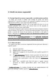
ρ(x,t)<br />
1.2<br />
1<br />
0.8<br />
0.6<br />
0.4<br />
0.2<br />
ε=1e−004, t=0.1, N=200<br />
0<br />
0 0.1 0.2 0.3 0.4 0.5<br />
x<br />
0.6 0.7 0.8 0.9 1<br />
σ(x,t)<br />
0.07<br />
0.06<br />
0.05<br />
0.04<br />
0.03<br />
0.02<br />
0.01<br />
0<br />
q(x,t)<br />
0.25<br />
0.2<br />
0.15<br />
0.1<br />
0.05<br />
0<br />
−0.05<br />
ε=1e−004, t=0.1, N=200<br />
−0.1<br />
0 0.1 0.2 0.3 0.4 0.5<br />
x<br />
0.6 0.7 0.8 0.9 1<br />
ε=1e−004, t=0.1, N=200<br />
−0.01<br />
0 0.1 0.2 0.3 0.4 0.5<br />
x<br />
0.6 0.7 0.8 0.9 1<br />
p(x,t)<br />
3.5<br />
3<br />
2.5<br />
2<br />
1.5<br />
1<br />
0.5<br />
0<br />
0 0.1 0.2 0.3 0.4 0.5<br />
x<br />
0.6 0.7 0.8 0.9 1<br />
u(x,t)<br />
1.8<br />
1.6<br />
1.4<br />
1.2<br />
1<br />
0.8<br />
0.6<br />
0.4<br />
0.2<br />
0<br />
ε=1e−004, t=0.1, N=200<br />
ε = 10 −4 , λ = 0.1, N = 200 at time t = 0.1.<br />
ε=1e−004, t=0.1, N=200<br />
−0.2<br />
0 0.1 0.2 0.3 0.4 0.5<br />
x<br />
0.6 0.7 0.8 0.9 1<br />
31
Lattice-Boltzmann models<br />
∂tf + v<br />
ɛ · ∇xf = 1<br />
ɛ 2 τ (f − f eq ), x, v ∈ R 2 ,<br />
v ∈ {c0, . . . , cN−1}, N = 9, ci ∈ {(0, 0), (0, ±1), (±1, 0), (±1, ±1)}.<br />
f eq �<br />
[ρ, u](v) = ρ 1 + 3u · v − 3<br />
2 |u|2 + 9<br />
�<br />
(u · v)2 f<br />
2 ∗ (v),<br />
ρ(x, t) =<br />
N−1 �<br />
i=0<br />
f(x, ci, t), ρu(x, t) =<br />
N−1 �<br />
i=0<br />
cif(x, ci, t),<br />
f ∗ (c0) = 4<br />
9 , f ∗ (ci) = 1<br />
9 , i = 1, ..., 4, f ∗ (ci) = 1<br />
, i = 5, ..., 8<br />
36<br />
As ɛ → 0 we obtain the incompressible Navier-Stokes equations with Reynolds number<br />
O(1/τ).<br />
shear layer<br />
(x, y) ∈ [0, 2π] 2 , ux(x, 0) = 0.05 sin(x), periodic b.c. and<br />
uy(x, y) = tanh(15(y − π/2)/π), y < π, uy(x, y) = tanh(15(3π/2 − y)/π), y > π.<br />
We test IMEX-SSP2(2,2,2) and IMEX-SSP3(3,3,2) <strong>schemes</strong> combined with second and<br />
third order upwind <strong>schemes</strong> based on CWENO reconstructions.<br />
32
Euler case (τ = 0): First order (left), Second order (center), Third order (right) at t=4<br />
with N = 64 (bottom) and N = 128 (top) <strong>for</strong> ε = 10 −6 .<br />
h = 1/128<br />
h = 1/64<br />
6<br />
6<br />
5<br />
5<br />
4<br />
4<br />
3<br />
3<br />
2<br />
2<br />
1<br />
1<br />
0 1 2 3 4 5 6<br />
0<br />
0 1 2 3 4 5 6<br />
0<br />
h = 1/128<br />
h = 1/64<br />
6<br />
6<br />
5<br />
5<br />
4<br />
4<br />
3<br />
3<br />
2<br />
2<br />
1<br />
1<br />
0 1 2 3 4 5 6<br />
0<br />
0 1 2 3 4 5 6<br />
0<br />
h = 1/128<br />
h = 1/64<br />
6<br />
6<br />
5<br />
5<br />
4<br />
4<br />
3<br />
3<br />
2<br />
2<br />
1<br />
1<br />
0 1 2 3 4 5 6<br />
0<br />
0 1 2 3 4 5 6<br />
0<br />
33
Navier-Stokes case (τ = 0.01): First order (left), Second order (center), Third order<br />
(right) at t=10 with N = 64 (bottom) and N = 128 (top) <strong>for</strong> ε = 10 −6 .<br />
h = 1/128<br />
h = 1/64<br />
6<br />
6<br />
5<br />
5<br />
4<br />
4<br />
3<br />
3<br />
2<br />
2<br />
1<br />
1<br />
0 1 2 3 4 5 6<br />
0<br />
0 1 2 3 4 5 6<br />
0<br />
h = 1/128<br />
h = 1/64<br />
6<br />
6<br />
5<br />
5<br />
4<br />
4<br />
3<br />
3<br />
2<br />
2<br />
1<br />
1<br />
0 1 2 3 4 5 6<br />
0<br />
0 1 2 3 4 5 6<br />
0<br />
h = 1/128<br />
h = 1/64<br />
6<br />
6<br />
5<br />
5<br />
4<br />
4<br />
3<br />
3<br />
2<br />
2<br />
1<br />
1<br />
0 1 2 3 4 5 6<br />
0<br />
0 1 2 3 4 5 6<br />
0<br />
34
Conclusions<br />
<strong>Runge</strong>-<strong>Kutta</strong> IMEX <strong>schemes</strong> represent a powerful tool <strong>for</strong> the time discretization of <strong>hyperbolic</strong><br />
<strong>systems</strong> with relaxation. In combination with finite volume <strong>schemes</strong> (up to second<br />
order) or finite difference <strong>schemes</strong> (of any order) they provide a new class of efficient<br />
underresolved <strong>schemes</strong> <strong>for</strong> the accurate solution of <strong>hyperbolic</strong> conservation laws with stiff<br />
source terms.<br />
Open problems and extensions:<br />
◦ 4th and 5th order IMEX-SSP <strong>schemes</strong><br />
◦ Higher order (more than third) finite volume <strong>schemes</strong> <strong>for</strong> <strong>hyperbolic</strong> <strong>systems</strong> with<br />
stiff relaxation<br />
◦ Less restrictive conditions <strong>for</strong> APk property<br />
◦ Development of well-balanced <strong>schemes</strong> that avoid numerical viscosity<br />
◦ Adaptive multi-modelling<br />
◦ Coupling with hybrid Monte Carlo strategies <strong>for</strong> multiscale problems.<br />
35