using Forward-looking Information - FKFS

Determination of Saving Potential 

for a Parallel Hybrid Power Train 

(using Forward-looking Information) 

Dipl.-Ing. Thomas Riemer, FKFS 

Dipl.-Ing. Tobias Mauk, IVK 

Prof. Dr.-Ing. Hans-Christian Reuss, IVK/FKFS

Abstract 

Anticipatory driving can lower fuel consumption of a vehicle. Because of the ability to store 

energy, anticipation is even more promising for hybrid power trains. The knowledge of the road 

to come (by means of digital road-maps) allows an energy optimal operation of the hybrid power 

train. 

An energy based investigation is not sufficient for potential-determination, because the degrees 

of freedom are limited by constraints. For a realistic determination of saving potentials, degrees 

of efficiency, storage space and maximum power of the components have to be considered. The 

potential of a forward-looking strategy of operation results from an optimal progression of 

control variables over the driving route. Control variables of a parallel hybrid power train are 

driving torques of combustion and electrical engine and chosen gear ratio. The determined 

energy consumption over the given route and given speed progression can be used as a benchmark 

for an implemented real-time strategy of operation. 

A concept for determination of optimal progression of control variables and thus a way to determine 

optimal energy consumption is introduced within this paper. The concept is demonstrated 

by a parallel-hybrid vehicle featuring a natural-gas combustion engine. 

1 Introduction 

Speaking about parallel-hybrid drive trains is sometimes difficult, because using the same vocabulary 

as for regular drive trains, consisting of combustion engine followed by one clutch and 

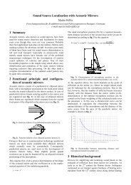
a gear-box, does not always apply to parallel-hybrid drive trains. The parallel-hybrid drive train 

examined in this paper (see Fig 1-1) consists of a combustion engine followed by a clutch, 

connecting it to an electrical engine, followed by a second clutch, connecting the engines to the 

gearbox. In this paper the clutch between combustion and electrical engine is referred to as 

clutch1. The clutch between the electrical engine and the gearbox is referred to as clutch2. The 

combination of combustion and electrical engine is referred to as the engine throughout this 

paper, as it replaces the combustion engine of a regular drive train.

Combustion 

engine 

Clutch1 

Engine 

Fig 1-1 Power train structure 

Determination of Saving Potential for a Parallel Hybrid Power Train 

Electrical 

engine 

Clutch2 

Gearbox 

To be able to determine fuel consumption (and thus CO2 exhaust) over a given route, the mechanical 

energy needed to drive the vehicle needs to be known. To determine the progression of 

the driving resistance, the elevation and speed progressions as well as certain parameters of the 

vehicle such as weight, wind drag coefficient, cross-sectional area and rolling resistance coefficient 

have to be known. From the progression of wheel speed and driving torque at the driving 

wheels the needed engine torque and engine speed for each gear can be calculated by a simple 

vehicle model. This is referred to as „backward simulation“ as the engine torque and speed are 

results of the vehicle speed, reversing the causal chain. 

Knowing the engine speed and torque needed throughout the route for each gear, the optimal 

way to meet these requirements (i.e. the required driving power) has to be determined. This is 

done by optimization methods resulting in vectors of gear ratio and electrical engine torque. 

2 Vehicle model 

To determine the required driving power throughout the driving route, a mathematical vehicle 

model has to be developed. As only energy consumption related issues are regarded, influences

y elasticity and play in the drivetrain can be disregarded. Thus the influences to be modelled 

are driving powers, degrees of efficiency of the electrical system and the CO2 emissions of the 

combustion engine. 

Driving powers 

The required driving power is dependent on the driving resistance at each time over the driving 

course. The driving resistance is the sum of the forces counteracting the vehicle movement 

(except the slope resistance that can support vehicle movement in case of downward slope): 

F = F + F + F + F 

dr 

rr 

wd 

a 

sl 

The driving resistance consists of the wind drag, rolling drag, acceleration resistance and slope 

resistance. These result in the driving resistance at the driving wheels. The driving resistance 

force has to be multiplied by the wheel diameter to determine the driving torque at the driving 

wheel. In addition to the wheel driving torque component resulting from the driving resistance, 

an additional torque component resulting from angular acceleration of the wheels has to be 

added. Although only 2 wheels are driven, obviously all four wheels have to be accelerated as 

the car drives on the road. So the torque of inertia of all 4 wheels has to be considered. 

τ = F × r + 4 J × & ω 

wh 

F dr … driving resistance 

F rr … rolling drag 

F wd … wind drag 

F a … acceleration resistance 

F sl … slope resistance 

dr 

wh 

wh 

wh 

τ wh … wheel driving torque 

F … driving resistance (3.1) 

dr 

r … wheel diameter 

wh 

J … moment of inertia of the wheel 

wh 

ω& … angular acceleration 

wh 

As only quasi-static driving states are regarded in this work, clutch slip is neglected. Thus the 

rotational speed relation between wheels and engine always equals the gear ratio. To determine 

driving torque at gearbox entry, the wheel driving torque has to be divided by the product of 

axle and gear ratio. Additionally the drive train efficiency has to be regarded. Although the 

(2.1) 

(2.2)


efficiency of a drive train has constant, speed and load dependent losses [2] , a constant relation 

between output and input power is appropriate for this kind of research. 

P 

out 

= P × η ⇒ ω × τ 

in 

ωout 

× τ out τ out 

τ in = = 

ω × η i × η 

in 

out 

n 

out 

= ω × τ × η 

in 

in 

As the diameters of drive-shafts and gearbox-shafts are low in comparison to wheel and engine 

diameters, their moment of inertia will be neglected in this research. Their moment of inertia 

could be added to the wheels or the engine, multiplied by the square of the ratio [1] As the 

consumption maps for the engines are measured in static operating points, their moments of 

inertia have to be accounted for in addition to the gearbox entry torque. As the required torques 

are calculated before the operation mode is chosen, it is not known if the combustion engine 

has to be accelerated or not (e.g. if clutch1 is open or closed). Therefore the moment of inertia 

of the combustion engine is always added, assuming it is always revolving. 

τ 

τ & 

wh 

en = + ωwh 

in 

× η 

en 

P in, 

out … in/output powers 

τ in. out 

ωin. 

out 

ω = ω × i 

wh 

n 

× i × J 

n 

ω … engine angular velocity 

en 

en 

τ en … required engine torque 

J … moment of inertia of the engine (engines + clutches) 

en 

… in/output torques 

… in/output angular velocity 

i … overall gear ratio in gear n 

n 

η … drive train degree of efficiency 

(2.4) 

(2.5) 

With 3.4 & 3.5 the required engine torque in all gears for a given course can be calculated. Fig 

2-1 shows the required engine torques in all the gears compared to the vehicle speed. 

(2.3)

Fig 2-1 required engine torques 

Electrical system 

Electrical engine 

The electrical system consists of the electrical motor and the battery. This combination makes it 

possible to transform mechanical energy into electrical energy and vice versa. The mechanical 

energy can be drawn from the combustion engine as well as the kinetic energy of the vehicle. 

For the electrical engine a characteristic map for the current has to be determined. To generate 

the map, a grid of torques and revolution speeds has to be established. The current for every 

point of that grid has to be measured. An example for such a map is shown in Fig 2-2. The 

current is measured at a defined constant voltage.

Fig 2-2 characteristic map of the electrical engine 


As the battery voltage will change with battery State-of-Charge (as from now abbreviated SoC) 

and battery current, electrical power has to be calculated from the current map by multiplying 

with the operation voltage used during current measurement. 

P ( τ , n) 

= I ( τ , n) 

× U 

em 

meas 

Using a degree of efficiency map is not appropriate for this purpose, as it depicts the relation 

between acquired mechanical power and electrical power. Regarding a start-up procedure, the 

mechanical power is zero as the angular speed is zero and so the product of angular speed and 

torque (mechanical power) is also zero. Still a current is required to produce this torque, making 

the degree of efficiency zero. This makes calculation of required current for a desired 

torque impossible, so a current map is needed. 

Battery 

(2.6) 

The battery model is based on the Randles battery model (Fig 2-3). This model is an origin for 

a variety of more complex models [3] As the simulation/optimization method is based on quasistatic 

states, the inductive and capacitive components are neglected. Thus only the SoC and the 

internal resistance will be modelled.

+ 

Fig 2-3 Randles battery model 

To model the battery terminal voltage, the dependency of voltage and SoC has to be determined. 

The terminal voltage has to be determined for a given SoC and given current. The SoC 

influence has to be modelled by a characteristic curve. 

Fig 2-4 Battery voltage curve 

L 

The terminal voltage is also influenced by the current through the internal resistance. 

R1 

C 

R2 

-

U = U ( SoC) 

+ I × R 

term 

i 


i 

The State of Charge is the integration of the current flowing into the battery, so a constant factor 

similar to the capacity of a capacitor can be determined. Although secondary batteries (e.g. 

NiMH batteries) used in hybrid-vehicles naturally discharge with time, this effect can be neglected 

for optimization runs spanning well under an hour. 

SoC( 

t) 

= Cbat 

× ∫ I( 

t) 

dt + SoC 

t 

t0 

Current calculation 

0 

To determine the SoC-change through equation (2.8) in dependance of the mechanical power of 

the electrical engine, the corresponding current has to be calculated. 

P 

I = 

U 

em 

term 

With (2.6, 2.7): 

Pem 

I = 

U + R × I 

i 

−U 

I = 

U term … terminal voltage 

U i … internal voltage (SoC-dependent) 

I … current (positive values mean loading) 

R i … internal resistance 

SoC … State of Charge 

SoC 0 … initial SoC 

C bat … equivalent battery capacity 

i 

+ 

i 

U 

2 

i + 

2R 

i 

4P 

em 

R 

i 

(2.7) 

(2.8) 

(2.9) 

(2.10)

Combustion engine 

For the determination of the carbon dioxide emissions of the combustion engine, an emissions 

map is needed. 

Fig 2-5 Exemplary CO2 emissions for a combustion engine 

3 Optimization 

Goal of this research is to find the optimal way to drive a given road route in respect of CO2 

emissions with a parallel-hybrid vehicle. Degrees of freedom for that task are the chosen gear 

and division of needed driving torque to the two engines. An appropriate optimization method 

to solve this problem is dynamic programming. It is based on the Bellman-equation. 

„An optimal policy has the property that whatever the initial state and initial 

decision are, the remaining decisions must constitute an optimal policy with 

regard to the state resulting from the first decision.“ – Bellman, 1957


This means that for each part of the solution vectors, the „sub“-solution has to be the optimalway 

between these two points. 

A B 

c=1 

1 

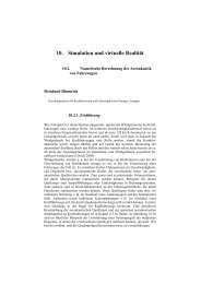
Fig 3-1 Dynamic Programming Step-by-step decision process 

Fig 3-1 illustrates the step-by-step decision process. For every state of the current step, the 

„cheapest“ sum of any state in the step before and the corresponding way to the current state in 

the current step has to be found. As there is only one state in the final step, the sum of the cost 

for the transition to the final state plus the overall cost to the preceding states decide the overall 

cost. So for every state in the current step only as many decisions as there are preceding states 

have to be made. So for n steps and x states the number of necessary decision is: 

2 

d = x × ( n − 3) 

+ 2× 

x 

The overall number of possible combinations calculates to 

−2 

= n 

c x 

2 

C D 

1 

c=1 5 

3 

c=5 2 

1 

c=7 

2 

c=2 

3 

c=2 

1 

c=3 4 

d … number of necessary decisions 

x … number of states 

n … number of steps 

c … number of combinations 

5 

c=6 

So for an optimization problem consisting of 200 steps and 100 possible states, using dynamic 

programming leads to 1.97 × 10 6 decisions, compared to 10 396 possible combinations. 

1 

2 

1 

2 

c=1 

3 

3 

c=2 

c=1 

c=2 

3 

3 

5 

1 

5 

1 

c=5 

c=3 

c=5 

1 

5 

c=3 

2 

4 

c=7 

c=6 

1 

3 

c=8 

(3.1) 

(3.2)

4 Problem modelling 

For comparability to production cars, the NEDC-cycle (New European driving cycle) was chosen 

(Fig 4-1). 

Fig 4-1 New European driving cycle 

To find the optimal way to drive a given route, an internal state of the system has to be chosen. 

In this case, the SoC of the battery was chosen. So the desired SoC-range is divided into an 

appropriate number of SoC-levels. The number of levels chosen is determined by the current 

necessary to go one step up/down within one time step. The current to in/decrease the SoClevel 

by one discrete step can be determined by transforming (2.8): 

SoC 

I 

C t Δ × 

Δ 

= 

bat 

Δ SoC … SoC-level unit interval 

Δ t … step width 

(4.1) 

The SoC- and time-resolution should be chosen in a way, that the current (and thus the electrical 

power at an average battery voltage level) necessary for a SoC-in/decrease by one step 

corresponds to a reasonable torque resolution in the torque range of the electrical/combustion 

engines even at lower rotational speeds. For this problem no general solution can be presented, 

as it depends on the regarded components. In the research this paper is based on, a step width 

of 0.5 s and a resolution of 1000 SoC-levels for 10 % SoC-range was chosen.


From the necessary driving torques (as calculated in Chapter 2), the driveable gears have to be 

determined. An important difference to the dynamic programming example shown in Chapter 

three is that the state transitions can be executed in different gears. So each transition has to be 

evaluated per driveable gear. This can be thought of as multivalued transitions. A gear is driveable 

if the sum of the maximum torques of both engines is higher than the required driving 

torque in that gear for positive (powering) torques. For negative torques (decelerating), all 

gears are possible as not all the torque has to be produced by the electrical engine. As the brake 

system of the car remains unmodified, only a part of the braking torque can be recuperated by 

the electrical system, so an upper torque percentage limit has to be defined. For the car this 

work is based on, the maximum torque regarded throughout the optimization procedure for the 

electrical engine equals a third of the decelerating torque needed. 

To allow battery loading during driving breaks (e.g. stops at traffic lights), an engine rotational 

speed is defined. It was set to 2500 rpm. This speed was chosen as the torque range is at its 

maximum and the area of optimal degree of efficiency is also located at that rotational speed. 

The minimum torque is set to zero, the maximum torque is the lower of the maximum torques 

of both engines. The required driving torque in this case is zero. 

Knowing the driveable gears, the maximum and minimum of the torque applicable for the electrical 

engine has to be determined. The maximum torque is the minimum selection of the torque 

the electrical engine can provide and the torque that is needed in the selected gear. The minimum 

torque is the difference between the required driving torque and the maximum torque the 

combustion engine can provide. 

τ dr ( i, t) 

− τ max_ ce ( n) 

< τ em ( t) 

< min( τ max_ em ( n), 

τ dr ( i, 

t)) 

τ dr … driving torque 

τ max_ ce 

τ max_ em 

… maximum torque of combustion engine 

… maximum torque of electrical engine 

i … gear 

(4.2) 

From the possible torque range and the rotational speed in the regarded gear, the electrical 

current limits can be calculated by (2.10). By solving (4.1) for Δ SoC , the possible amount of 

SoC in/decrease steps for this time step and the regarded gear can be determined. As not all 

transitions between states of adjacent steps are possible because of the limited SoC in/decrease 

range, the theoretical complexity calculated with (3.1) is by far beyond the necessary number of 

calculations. Thus the computation time for this method is acceptable for theoretical research. 

With the possible SoC-level step range, the necessary electrical engine torques for the exact 

current to make the desired SoC-level steps have to be determined by reversing the characteristic 

map for the electrical engine (Fig 2-2) to provide torque from given rotational speed and 

current. 

The difference between the necessary driving torque and the electrical engine torque equals the 

necessary combustion engine torque. By looking up the emitted CO2 for the current rotational 

speed and the determined necessary torque fraction for the combustion engine in Fig 2-5, the

„cost“ for the regarded route leading to this specific state (SoC-level) can be calculated by 

adding the so-far emissions to the origin state of the current consideration. If no better state 

vector had been found, the state and gear vector as well as the CO2 emissions are stored for the 

regarded destination state. For simplicity reasons, the electrical engine torque vector is also 

stored, although it could be reconstructed from the SoC-level and gear vectors after the optimization 

is done. 

5 Results 

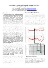
After the optimization run, the following results were derived. Fig 6-1 shows an excerpt of the 

progression of the regarded vectors. Shown are the required torque in the gear selected during 

the optimization run and the optimal electrical engine torque vector, the acquired gear and the 

SoC progression. 

The results feature multiple kinds of hybrid operating modes. During braking manoeuvres, 

kinetic energy is regained by recuperation. At constant velocity, the combustion engine operating 

point is shifted to higher loads by producing negative torque. This way the battery is 

charged. The stored energy is used to support the combustion engine, making it possible to 

select a higher gear. 

It is obvious that the result shows the discharge of the battery just before it is recharged at the 

long deceleration manoeuvre at the end of the cycle. Recuperation is always done when possible. 

The CO2 emissions determined for the used middle-class caravan were about 88.27 g CO2/km. 

Compared to the production car (1.6 liter gasoline engine, no hybrid), emitting approximately 

150 g CO2/km, the potential is significant. Still there would be compromises to be made in 

respect of driveability, comfort and comprehensibility, so a production car featuring the components 

simulated in this research would emit more CO2/km than the calculated value. 

6 Conclusion 

The chosen optimization approach is well suited for the given problem. It is a good way to 

determine the potentials for a given hardware configuration. It can also help in developing an 

appropriate strategy of operation and to evaluate an already established solution. Further research 

is required to fully understand the determined optimal solution. 

For a real-time implementation of the described method, the computation times are problematic. 

Depending on the valid SoC-range, SoC-resolution and the regarded horizon, real-time 

calculation can become impossible [5] . An operation strategy for a vehicle with a high-capacity 

battery, making it possible to use electric drive for longer periods, has to regard a far optimization 

horizon. Using neural networks, trained to deliver the results, the offline optimization 

would have, could be a solution to this problem.


Fig 6-1 Optimization results, electrical engine torque, gear & SoC

Bibliography 

[1] Trägheitsmoment/Übersetzung, R. Isermann, Springer 2002 

[2] Powertrain Performance vs. Engine Performance, 

White Paper, Rototest Research Institute, 2005 

[3] Electrochemistry, Carl H. Hamann, Andrew Hamnett, Wolf Vielstich, 

WILEY-VCH, 2007 

[4] Optimal Control, Richard Vinter, Birkhäuser Boston, 2000 

[5] Prädiktive Antriebsregelung zum energieoptimalen Betrieb von Hybridfahrzeugen, M. 

Back, Dissertation, Universitätsverlag Karlsruhe, 2005

using Forward-looking Information - FKFS

Create successful ePaper yourself

Delete template?

Save as template?