An incremental learning method for foresight information ... - FKFS

An incremental learning method for
foresight information used in predictive
driving strategies
M. Sc. Anne Carlsson, University of Stuttgart, IVK, Automotive Software and Mechatronics
Prof. Dr.-Ing. H.-C. Reuss, University of Stuttgart, IVK, Chair of Automotive Mechatronics

Abstract
Abstract
It has often been shown that foresight information can improve fuel efficiency and comfort
functions as well as active and passive safety systems. In this paper it will be shown how a
database containing roadside information of a frequently driven route can be automatically
generated and continually updated in the vehicle during the drive. The identified road
characteristics such as curves, slopes, and speed information can be used as prediction or
foresight information in subsequent drives along the route. The situation identification
algorithms used in the system presented here base on standard sensors found in vehicles
equipped with an electronic stability system and ABS. Additionally a positioning system such
as GPS is required to define the geographical position of the identified road or traffic situation.
An identified event such as a curve in the road or a steep uphill section can in terms of memory
capacity be efficiently described with a set of attributes; geographical position, magnitude,
number of observations, and date and time information of the observation. This information
can be stored in a vehicle individual database with an analogous structure. During each drive
this database can be continually extended and updated by comparing newly identified events
with equivalent events already existing in the database. The development of the identification
and comparison algorithms described here bases on real test drive data, performed through
funding from the Geschwister-Heine Foundation and the Friedrich- und Elisabeth-Boysen
Foundation.
1 Introduction
Since the ABS (anti-lock braking system) became available, driver assistance systems continue
to have a central part by the development of new vehicles. A variety of (assistance) systems for
increased comfort, safety and fuel economy have since then been introduced in the vehicles.
Some systems worth to mention are Adaptive Cruise Control (ACC), Advanced Front Lighting
(AFL), systems for predictive gear shifting, electronic stability systems and curve speed
warning etc. [15][16][19]. All these systems base on additional sensor integrated in the vehicle.
These sensors measure the actual state of the vehicle and the systems can react accordingly.
Many previous research projects have shown that with information about the road ahead, i.e.
foresight information, the function of some of these systems could be greatly improved
[2][3][18]. These systems usually base on the expectation that future digital maps will contain
the necessary three dimensional road information or that the required information will be
available through communication with intelligent infrastructure [4][22]. Today however, a
great amount of roadside information relevant for these applications is still lacking. The major
challenge for the map vendors is the collecting of data and keeping it up to date for a useful
support [5][17]. This turns out to be both difficult and expensive. During the years some
projects were initiated to find methods to gather the information needed. Some of the methods
base on so called floating car data [1][6], others on additional sensors fitted to the vehicle, e.g.
radar and cameras [7][14].

Curvature
In this paper a further method for the collecting and actualisation of foresight information will
be discussed. The method bases on the fact that many vehicles repeatedly travel the same route,
i.e. commuter vehicles, public transport or commercial vehicles. With this approach the system
can “memorise” or “learn” the characteristics of the driven route – just as an observant driver
would do. The learnt information can then be used as foresight information in subsequent
drives along a particular route – just as the forward looking driver would do. Possible fields of
application, beside fuel efficient power train control, could be improved curve speed warning,
adaptive headlight control and predictive gear selection, as well as improved controlling of the
energy flow in hybrid powered vehicles.
The approach presented here claims to be cheaper and more flexible than many other systems
in this category. The reasons for this are that the system only employs sensors counting more
or less to standard equipment in the vehicles today, and that the collected information is limited
to but focused on the part of the road network where the vehicle is primarily moved. Hence the
amount of data to be stored can be limited to the, for a particular vehicle / driver, truly relevant
information.
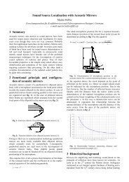
In Figure 1 a flow diagram describing the process of a learning vehicle for forward-looking
driving can be seen. During a drive sensors, e.g. yaw rate and acceleration sensors, gather
information about vehicle movements and road characteristics along the travelled road. The
gathered data are directly analysed and features in the measurement data indicating relevant
situations are extracted. With the positioning system each identified situation (a so called
“event”) can be associated with a geographical position. Based on this position, the new event
data are compared to the data of equal event types identified at the same geographical position
during previous drives, i.e. data already existing in the vehicle internal database. If the
compared events correlate the database is updated accordingly. On the other hand, if no
parallels can be identified, the new data are simply added to the database as a new event. The
updated or added data will then in a similar way be involved in future comparisons with newly
identified events. Each time the database is updated, a status or counter value for the revised
event is incremented. This attribute gives information about the probability that the identified
situation is correctly recognised. The information in the database from events marked as “true”
can be released as foresight information for different control applications in the vehicle. The
main focus of this paper stays on the learning process itself, i.e. the updating of the database
containing the roadside information.
2 Implementation of the Learning System
The learning system presented here is implemented in C++ with a direct interface for reading
from the CAN bus of the host vehicle, currently using the API provided from Vector
Informatik GmbH. The identified event data is stored in a database based on MySQL. A
graphical display of the result is implemented with Qt® by TrollTech. The ambition is to
develop a system capable of real-time application and to be independent of platform. The
development of the system algorithms bases on real measurement data, collected during test
drives over several thousands of kilometres. The realisation of the learning system is
financially supported by the Geschwister-Heine Foundation and the Friedrich- und Elisabeth-
Boysen Foundation.

Learning
Process
Figure 1: Flow diagram for a learning vehicle for forward-looking driving
3 Situation detection
Situation detection
The situation detection algorithms for the learning system presented in this paper base apart
from engine control and drive train information only on standard sensors found in vehicles
equipped with e.g. ESP and ABS. I.e. sensors for longitudinal and lateral acceleration, yaw
rate, wheel speed and steering wheel angle. To be able to geographically position the identified
situations along the route, also a positioning system such as GPS, or in the next future the
Galileo system, is necessary [9].
For clarification purposes a couple of definitions used throughout this paper will be introduced;
a curve, a slope or a change in speed limits along the investigated road section will be referred
to as a specific situation type. As a road section could contain several occurrences of a
particular situation type, a single occurrence will be referred to as an event of a defined
situation type.
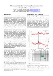
The diagrams in Figure 2 illustrate some signals measured during a number of independent
drives as function of the driven distance. The repeated pattern of the signals indicates that the
characteristics of the driven road section can be found by inspecting data from a number of
drives.
3.1 Curvature
Sensor Data Data
Conditioning
Situation
Verification
DB
Route
Characteristics
Situation
Identification
Applications using
foresight information
Data Fusion
Feature
Extraction
With the previous mentioned sensors, the curvature of a driven road section can be determined
in various ways. One possibility would be to use the lateral acceleration of the vehicle. Fitted
to the vehicle, such sensors would measure the total lateral acceleration of the vehicle and

Curvature
would hence include the lateral gradient of the road. Without information about this quantity,
the curvature determined from the lateral acceleration would only be valid along levelled road
sections. Another possibility would be the steering wheel angle. This measurement though, is
in addition sensitive to e.g. side wind, therefore not always reliable. A third option would be to
use the information from the yaw rate sensor. Assuming that the examined test drives were
conducted without skidding, it has been shown that the curvature of the driven road can be
satisfactorily identified using solely the information from the yaw rate sensor.
curvature [m -1 ]
velocity [m/s]
lat acc [m/s²]
long acc [m/s²]
30
20
10
0
0 1000 2000 3000 4000 5000 6000
4
2
0
-2
-4
0 1000 2000 3000 4000 5000 6000
4
2
0
-2
-4
0 1000 2000 3000 4000 5000 6000
0.01
0
-0.01
0 1000 2000 3000
distance [m]
4000 5000 6000
Figure 2: Some of the signals investigated for situation identification. The repeated pattern from
different drives indicates that the characteristics of the driven road to a certain extent can be
determined.

3.2 Road gradient
Data reduction
The longitudinal gradient, i.e. the slope, of the driven road can theoretically be identified using
information about the total longitudinal acceleration of the vehicle, together with the
acceleration of the vehicle due to the selected velocity. This measurement though, is sensitive
to e.g. noise, the pitch motion of the vehicle and the oscillations induced through interruption
in the traction force. In [11], [19] and [20] further methods for the determination of the road
gradient based on state observers are discussed.
3.3 Speed limit
While driving in urban areas the freedom of selecting speed and driving manner is usually
strongly limited. Looking at the velocity data in Figure 2, it can be seen that the velocity
chosen by different drivers and at different drive occasions along a certain road section have a
high level of agreement. This means that the appropriate velocity can be pretty well estimated
for this road segment. However, the selected speed may vary with both weekday and daytime.
I.e. a lower speed might be more appropriate at rush hour compared to the speed selected (or
allowed) at times for lower traffic density. Hence the time and date information of the drive is
required. Also information about the type of road is relevant for making a suitable estimate of
the valid speed limit. It has been shown that with information of selected gear, number of
standstills, standstill time, and maximum and minimum speed over a certain road segment, an
adequate rating of the road type can be made, e.g. motorway, highway or urban area.
Other interesting “situations” that can be recognised using only the previously mentioned
sensors are the positions for traffic lights and intersections. However, further discussions about
situation detection methods go beyond the scope of this paper. In [8], [12] and [13] are some
supplementary methods for situation identification and sensor fusion discussed.
4 Data reduction
At the bottom of Figure 2 the road curvature calculated from yaw rate and velocity information
for 4 independent drives along the same road section is shown. It can be seen that the
calculated curvature is similar throughout the drives. This indicates that the probability is high
that a situation, i.e. a curve, can be correctly identified in all drives. A curve event is detected
when the absolute value of the curvature exceeds a set limit. It can also be seen that the
curvature or curve radius hardly ever stays constant throughout the whole curve. Hence it is not
sufficient to represent a curve with just a single value for the curve radius. The application
“curve light” requires for example information about the actual curvature along the whole
extent of the curve for an appropriate adjusting of the head lights. To allow for this, the
complete measurement data of the identified event need to be stored in the vehicle internal
database. However, this would require great memory resources for each single event. The same
problem would also apply for slopes and speed limit changes.
To be able to store the data of the identified events in a memory efficient way, the amount of
measured data points needs to be reduced, however without loosing information. Instead of

Speed limit
storing all measurement values, the observations may be described through a mathematical
model whose characterising parameters can be stored. This so called curve fitting method also
works as a kind of filter on the observations to remove too large and unrealistic variations in
the measurement data. This is valid under the assumption that situations of this type (curves,
slopes, etc) in the reality have a smooth characteristic. As a result each set of measurement data
can be described with only a few values, i.e. the parameters of the specified approximation
function. The difficulty with this method is the automatic selection of a suitable fit function,
linear or nonlinear, and its degree. No graphing or analysis software can pick a model for the
given data – it can only help in differentiating between models. With a certain understanding of
the underlying properties of the measurement data, an adequate model can be chosen. Through
an analysis of the observations, in terms of e.g. local and global minima and maxima, a
decision of the model type and degree can be made. As can be seen in Figure 3, each identified
event of a certain situation type can be approximated with a linear or a nonlinear function of a
specific degree, e.g. a polynomial or rational function, without too much loss of information.
Each fit, i.e. each approximation, can be validated through analysing the Goodness of Fit. And
when necessary, the fit is repeated with a slightly different model until a satisfying result is
achieved. The Goodness of Fit (GOF) gives a measure on how good a statistical model fits a
set of observations (true values). The GOF typically summarises the discrepancy between
observed values and the values predicted under the model in question. For this application the
GOF analysis includes 4 measures; the sum of squares due to error (SSE), statistics on how
successful the fit is in explaining the variation of the data (R²), a measure for the quality of the
fit when adding additional coefficients to the model (adjusted R²) and finally the root mean
squared error (RMSE). For a good fit SSE and RMSE should be close to 0, and R² and adjusted
R² should be close to 1.
The real measurement data for some events shown in Figure 3 together with the
approximations are summarised in Table 1. In the table the identified curves and their fit
functions are listed together with the result of the goodness of fit analysis. Rat 55 means a
rational function with both numerator and denominator of degree 5. Poly 9 means a polynomial
of degree 9. According to this method, the only data that need to be stored in the database for
each event of a specific situation type are the start and end positions, the length, the type of fit
model, the degree of the used fit model and the result, i.e. the parameters, of the fitted function.

curvature [m -1 ]
curvature [m -1 ]
curvature [m -1 ]
0.2
0.15
0.1
0.05
0.02
0.015
0.01
0.005
curve 1
rat55
0
0 10 20 30
0
160 170 180 190 200
0
-0.005
-0.01
poly7
curve 3
curve 5
poly8
-0.015
240 260 280
distance [m]
300 320
0.05
0
-0.05
-0.1
-0.15
curve 2
Data reduction
poly9
-0.2
60 70 80 90
0.08
0.06
0.04
0.02
poly6
curve 4
0
220 230 240 250
x 10-3 curve
-2
-3
-4
6
poly7
-5
360 370 380 390
distance [m]
Figure 3: Curve fitting. Real measurement data (red) approximated with different linear and nonlinear
models (blue). Rat55 = rational function of degree 5 over degree 5, poly9 = polynomial
function of degree 9.

Speed limit
Table 1: Summary of curve fitting and goodness of fit analysis for the real measurement data
shown in Figure 3
Curve Fit Function SSE R² Adj. R² RMSE
1 Rat 55 0. 0046 0.9971 0.9970 0.0032
2 Poly 9 0.0098 0.9677 0.9659 0.0079
3 Poly 7 1.77e-5 0.9974 0.9973 3.24e-4
4 Poly 6 4.15e-4 0.9968 0.9968 0.0013
5 Poly 8 2.09e-5 0.9922 0.9920 2.85e-4
6 Poly 7 2.30e-6 0.9247 0.9193 1.54e-4
5 Database structure
For each identified event, i.e. a specific curve or slope along the driven route, only a few
attributes need to be stored (for future use) in the vehicle internal database; start position, end
position, geographical length of the event, type of fit model, degree of fit function, and the
characterising fit parameters. The structure of the implemented database is shown in Figure 4.
Beside the above mentioned attributes, each event has also a date and time stamp and a counter
variable.
The date and time information of the events have two purposes. The first one is to account for
the differences in some of the identified events due to week day and time of the day, e.g.
recommended or suggested velocity at rush hour compared to times with a lower level of
traffic density. The second purpose with the date information is to be able to keep the whole
database up to date. Too old elements in the database without a recent update can be removed
from the database after a certain time, e.g. 6 months.
The counter variable for each event is important to keep track on how many times a certain
event at a certain geographical position was identified in an equivalent way. The value of the
counter together with the total number of drives along a certain route, give the probability that
this event was accurately identified. If the probability is high, the event can be approved as
valid foresight information and can be released for usage in assistance systems.

Table: CurveCtrl
RouteNo
CurveNo
Table: Route
Table: SlopeCtrl
Table: SpeedCtrl
Table: Curve Table: Slope Table: Speed Table: TrafLight
Key: CurveNo
Curve_StartPos_X
Curve_StartPos_Y
Curve_EndPos_X
Curve_EndPos_Y
Curve_Length
Curve_DriveDir
Curve_FitFunction
Curve_Param
Curve_Date
Curve_Counter
RouteNo
SlopeNo
Key: SlopeNo
Key: RouteNo
Route_StartPoint_X
Route_StartPoint_Y
Route_EndPoint_X
Route_EndPoint_Y
Route_Length
Route_Date
Slope_StartPos_X
Slope_StartPos_Y
Slope_EndPos_X
Slope_EndPos_Y
Slope_Length
Slope_FitFunction
Slope_Param
Slope_Date
Slope_Counter
Route_Counter
RouteNo
SpeedCtrlNo
Key: CurveNo
Speed_StartPos_X
Speed_StartPos_Y
Speed_EndPos_X
Speed_EndPos_Y
Speed_Length
Speed_Value
Speed_Time
Speed_Date
Speed_Counter
Database structure
Table: TrafLightCtrl
RouteNo
TrafLightNo
Key: TrafLightNo
TrafLight_StartPos_X
TrafLight_StartPos_Y
TrafLight_EndPos_X
TrafLight_EndPos_Y
TrafLight_Value
TrafLight_Time
TrafLight_Date
TrafLight_Counter
Figure 4: Database structure used for storing and managing information from events identified
during a drive.
The database structure allows the system to contain several separate events of various situation
types for one specific route, as well as a number of different routes. The various routes could
for example be categorised as home – workplace, home – food store, workplace – fitness studio
or home – grandparents’ home. The motivation for this is that just as a single route could
contain many events of each specific situation type, one specific event could also appear in

Speed limit
more than one of the separate routes (in case some sections of the routes coincide). Using the
database structure presented here each event will exist only once in the database, but could still
be associated with several routes.
6 Event comparison
To keep the database up to date during each drive, it is necessary to compare the existing
entries in the database with the newly identified ones. If required, the existing database entries
are changed according to the new information, otherwise the new data is simply added to the
database as a new piece of information. The sensor data is evaluated online during the drive.
When an event is recognised, the relevant measurement data is stored temporarily until the
whole event is recorded. The next step is to compare this data with previously collected data.
This comparison can be performed “offline” but during the drive, basically while waiting for
the next event to occur.
Each time a new event is recognised during a drive, a search algorithm is started in the
database to find all comparable events already in it. The search algorithm is fed with the
situation type and the geographical start and end positions of the new event, e.g. “curve
beginning at position (xstart,ystart) and ending at position (xend,yend)”. Some curve events
identified during two separate drives along a defined road section are illustrated in Figure 5.
The three identified curves are found at approximately the same geographical position in both
of the drives. The circles represent the accepted tolerance of the start and end positions when
searching the database for comparable events. Both curve number 2 and curve number 3 have
the start and end positions within the tolerance while curve number 1 has none within the
tolerance.

Latitude [°]
48.748
48.748
48.747
48.747
48.746
curve 1
curve 2
curve 3
Event comparison
1st drive
2nd drive
9.1100 9.1105 9.1110 9.1115 9.1120
Longitude [°]
9.1125 9.1130 9.1135 9.1140
Figure 5: Evaluation of matching start and end positions of independently identified events
If one or more events of the requested situation type are found in the database with the start or
end position within the range of tolerance of the searched position, these events are retrieved
from the database to be individually compared with the newly recognised event. The
comparison to check the correspondence of the event data is done by checking the correlation
between the two sets of data. The correlation of two data sets is calculated according to
equation 1, where σX denotes the standard deviation and cov ( X , Y ) is the covariance of these
two variables.
( X , Y )
cov
R(
X , Y ) = (1)
σ σ
X
Y
The result of a correlation, the correlation coefficient, R, ranges from -1 to 1. The closer R is to
+1 or -1, the more closely the two variables are related. If R is close to 0 there is no
relationship between the variables. If R is positive, it means that as one variable gets larger, the
other gets larger. If R is negative, it means that as one gets larger, the other gets smaller. When
the correlation coefficient for the compared events is larger than a given threshold value (close
to 1), it can be assumed that the variables are representing the same event in the same way.
Otherwise it has to be assumed that the event was measured / identified in a different way in
the two independent drives. To determine the correlation it is necessary to calculate the
predicted data, based on the parameters of the approximating model. This is done by evaluating
the fit function for each of the events to be compared with its respective parameters, start
values and end values for a certain resolution. The correlation information for the curves
shown in Figure 5 are summarised in Table 2. The correlation coefficients of the data sets
representing the second and third curve event respectively are close to 1. Hence the
relationship between each of the two curve measurements is statistically confirmed. In Figure 5

Speed limit
it can be seen that curve number 1 was identified as a much longer curve during the second
drive compared to the first drive and consequently the correlation coefficient is low.
Table 2: Summary of correlation information for three different events identified during two
independent drives
Curve number Data set Fit function Correlation
coefficient
1 1 st Drive Poly 7 0.2235 No
2 nd Drive Poly 7
2 1 st Drive Poly 6 0.9734 Yes
2 nd Drive Poly 6
3 1 st Drive Poly8 0.9081 Yes
2 nd Drive Poly6
7 Database update
“Good
Correlation”
In Figure 6 a flow diagram showing the update process of the database can be seen. The
comparison of the two data sets is carried out by examining the correlation of the data. As
discussed in the previous section, it can be assumed that two sets of data represent the same
event when the calculated correlation coefficient is larger than a set threshold value. In this
case (following the left hand branch of the flow diagram in Figure 6) the examined entry found
in the database should be updated with a combination of the information from both events,
thereby not loosing any significant information. The start position of the updated event can be
set as the mean value of the beginning positions of the data sets to be combined. In the same
way the new end position can be determined. The process for the combining of the two sets of
approximated measurement data is not trivial and will be further explained below. When all
attributes of the event are newly determined, the examined entry in the database is updated
accordingly. Finally the counter of the updated event is increased with 1.
If the correlation coefficient on the other hand is lower than the set threshold value (right hand
branch), it can be assumed that the new event is differently measured than in previous drives,
or that a completely new event was found (at the same geographical position as an earlier event
of this type). Consequently this new event should be added to the database “as is”, as a new
entry. In this case its counter is set to 1, which indicates that the event was measured /
identified in this particular way for the first time. Also this conflicting data need to be stored,
as it could imply a change in road or traffic conditions.

Event data
from DB
Combine EvDB & EvCurrent
� EvUpdate
Set EvUpdate.counter =
EvDB.counter+1
Replace EvDB in database
with EvUpdate
Calculate
Correlation R
Yes No
R > limit
Figure 6: Flow diagram for the process of updating the database
Event data from
current drive
Set EvCurrent.counter = 1
Store EvCurrent in DB
Database update
When two compared events are found to correlate, their data sets need to be combined into one.
The details to the highlighted box in Figure 6 are shown in Figure 7. It represents a method for
merging two sets of event data. Principally an (weighted) average of the examined data needs
to be created. In the trivial case, the same approximation model was used to approximate the
real measurement values for both of the events (curve number 2 in Table 2). In this case the
new parameters can simply be calculated as an element wise average of the parameters for the
compared events. In the non-trivial case different fitting models were used for the
approximation (curve number 3 in Table 2). In this case an average of the predicted values
needs to be formed and it is required to carry out a new fitting process to obtain a new
parameter set describing the averaged data. For the curve fitting, the approximation models
used for each of the compared events are considered. The new fitting function is selected as the
one approximation giving the best result of the goodness of fit analysis.

Speed limit
Event data
from DB
Yes No
Same fit
function ?
Calculate average of
fit parameters for
EvDB & EvCurrent
Replace fit parameters of
EvDB with new fit
parameters
Retrieve fit functions
Fit average with
fit model 1
Calculate GOF
for Fit 1
Yes
Replace fit parameters of EvDB with
new parameters from Fit 1
Calculate average of
predicted values of
EvDB & EvCurrent
GOF1 better
than GOF2 ?
Event data from
current drive
Fit average with
fit model 2
Calculate GOF
for Fit 2
Replace fit parameters of EvDB with
new parameters from Fit 2
Figure 7: Flow diagram showing the combining process of two correlating data sets.
No

8 Results
Results
The result of the database updating process is illustrated in Figure 8. The event information
bases on measurement data from four different test drives. The thickest lines represent events
identified in an equal manner in 3 of the 4 examined test drives. The thinner the lines the fewer
are the times that a certain event was recognised in an equal way.
In the lower right diagram it can be seen that even though some of the events look very similar
they were still recognised as different events (at the same geographical position). This
problematic arises as the set limits for what “a good correlation” is or for when “a matching
starting point” are found, are hard coded. Using a fuzzy approach for the decision making of
when two sets of event data agree could solve this problem.
In the lower left diagram, the first curve was recognised in one manner 3 of the times and in
another manner 2 of the times, although only a total of 4 test drives have been examined. This
phenomenon can also be explained through the set limits for when a pair of event data are
categorised as equal. If the limit is set for event data to have at least 85% agreement to
continue the process of combining the examined event data, events with an agreement of
“only” 84.9% would be categorized as different events and hence not combined into one. Due
to this an event with a correlation close to, but below the set limit for e.g. a “good correlation”
is added to the database as a new event. As a result similar events identified during later drives
can have more than one matching event in the database. Each of the matching events found in
the database are compared with the newly identified one and updated according to the methods
illustrated in Figure 6 and Figure 7.
9 Outlook
A database for roadside information generated through the method discussed in this paper will
be individual for each vehicle and dependent on the travel pattern of the driver. Hence the
vehicle will lack foresight information each time a never driven route is selected. Especially for
long distance transport, a sharing system of the learnt information would improve its
functionality. As a result a new vehicle in a fleet or a new driver could immediately make use
of already learnt roadside information collected from another driver/vehicle, without having to
travel the route even once.
Making use of further sensors (preferably already available in the vehicle anyway), such as
short and long range radar or cameras for lane detection and night-view, would open up the
possibility for extended situation detection. In this case the information quality could be greatly
improved.

Speed limit
curvature [1/m]
curvature [1/m]
0.25
0.2
0.15
0.1
0.05
-0.05
0
-0.1
0.15
0.1
0.05
-0.05
0
-0.1
0 100 200 300
distance [m]
400 500 600
0 20 40
distance [m]
60 80
0.08
0.06
0.04
0.02
-0.02
0
1 time
2 times
3 times
200 250
distance [m]
300
Figure 8: Result of the database updating algorithm. Some of the events were even identified in a
similar way during all four of the examined test drives.

10 Bibliography
Bibliography
[1] Netzausgleich Individualverkehr NIV, Result report of sub-project. INVENT –
Intelligent traffic and user-friendly technology, www.invent-online.de. 2005
[2] Neunzig, D.; Benmimoun, A.: Potentiale der vorausschauenden Fahrerassistenz zur
Reduktion des Kraftstoffverbrauchs. Proceedings 11th Aachener Colloquium Fahrzeug-
und Motorentechnik, p. 1205-1238, 2002.
[3] Hettich, G.: Wise foresight. paper, DaimlerChrysler Innovation Symposium, Stuttgart,
2002.
[4] Brandstaeter, M.; Prestl, W.; Bauer, G.: Functional Optimization of Adaptive Cruise
Control Using Navigation Data. Paper. Proceedings SAE International, 2004.
[5] Herrtich, R. G.: Digital Road Maps Reveal the Telematic Horizon. Article. ITS America
News, Vol.12 No. 8, 2002.
[6] Lorkowski, S.; Brockfeld, E.; Mieth, P.; Passfeld, B.; Thiessenhusen, K.-U.; Schäfer,
R.-P.: Erste Mobilitätsdienste auf Basis von „Floating Car Data“. Proceedings for 4th
Aachener Colloquium "Mobilität und Stadt", Stadt Region Land, 75, p. 93 - 100,
Aachen (Germany), 2003, ISBN 3-88354-140-0.
[7] Wisselmann, D.; Gresser, K.; Spannheimer, H.; Bengler, K.; Huesmann, A.:
ConnectedDrive – ein methodischer Ansatz für die Entwicklung zukünftiger
Fahrerassistenzsysteme. BMW Group Forschung und Technik. Proceedings for
Conference Aktive Sicherheit durch Fahrerassistenz, Garching, 2004
[8] Naab, K.: Sensorik- und Signalverarbeitungsarchitektur für Fahrerassistenz und aktive
Sicherheit. Proceedings for Conference Aktive Sicherheit durch Fahrerassistenz,
Garching, 2004.
[9] Zogg, J.-M.: Von GPS zu Galileo – Die Weiterentwicklung der Satelliten-Navigation.
Teil 2: Galileo: Technik und Anwendungen. Article. Elektronik, No. 5, p. 50 – 56,
2006.
[10] Carlsson, A.; Reuss, H.-C.: A Learning Vehicle for Forward-Looking Driving. Paper.
Proceedings VDI conference Steuerung und Regelung von Fahrzeugen und Motoren.
VDI-Bericht 1931, p.109-119, 2006
[11] Hauke, M.: Adaptive Erkennung der Straßenneigung, Thesis work. Inst. für
Verbrennungskraftmaschinen und Thermodynamik, Technical University of Graz,
2003.
[12] Müller, M.; Reif, M.; Pandit, M.; Staiger, W.; Martin, B.: Vehicle Speed Prediction for
Driver Assistance Systems. Paper. Proceedings SAE International, 2004.
[13] Schammer, A.: Entwurf von Fusionsobjekten für den Einsatz in
Fahrerassistenzsystemen. Thesis work. Accomplished at DaimlerChrysler AG, Research
Division FT3/AA, University of Stuttgart, 2001.
[14] Schmitt, M.; Lorenzen, T.: Visuelle Verkehrszeichenerkennung mit dem Blackfin.
Article. Hanser Automotive, No. 11, p.14-19, 2006.

Speed limit
[15] Amsel, C.; Himmler, A.: Adaptive Lichtregelung: Lichttechnische
Fahrerassistenzsysteme. Article. Hanser Automotive, No. 7-8, p. 36-39, 2006.
[16] Wallaschek, J.; Locher, J.; Strauß, S.: Lichttechnische Fahrerassistenz. Article. ATZ,
No. 3, p. 204-211, 2006.
[17] Khan, M. S.; Herbst, M. R.; Sabel, H.: Erweiterte Datenbasis von Navigationskarten für
Fahrerassistenzsysteme. Proceeding for 9th Aachener Colloquium Fahrzeug- und
Motorentechnik, p.643-652, 2000.
[18] Back, M.; Terwen, S.: Prädiktive Regelung mit Dynamischer Programmierung für
nichtlineare Systeme erster Ordnung, Article, Automatisierungstechnik 51, No. 12, p.
547-554, 2003.
[19] Eder, J.; Birner, I.; Schloen, O.; John, T.; Nageleisen, F. : Sequentielles M-Getriebe der
zweiten Generation mit Drivelogic. Article. ATZ, No. 2, p.154-163. 2002.
[20] Halfmann, C.; Holzmann, H.; Isermann, R.; Hamann, C.-D.; Simm, N.: Adaptives
Echtzeitmodell für die Kraftfahrzeugdynamik. Article. ATZ, No. 12, p. 994-1001, 1999.
[21] Eschke, S.; Ploeger, G.: Automotive Applications using satellite based positioning.
Bosch. MSAA Conference, Brussels, 2006.
[22] Schupfner, M.; Artmann, K.: Optimierte Routenkalkulation bei Navigationssystemen.
Article. ATZ elektronik, No. 1, p. 54-61, 2006.