(voc) gas leak detection by using infrared sensors - Bilkent University

VOLATILE ORGANIC COMPOUNDS (VOC)
GAS LEAK DETECTION BY USING
INFRARED SENSORS
A THESIS
SUBMITTED TO THE DEPARTMENT OF ELECTRICAL AND
ELECTRONICS ENGINEERING
AND THE INSTITUTE OF ENGINEERING AND SCIENCE
OF BİLKENT UNIVERSITY
IN PARTIAL FULFILLMENT OF THE REQUIREMENTS
FOR THE DEGREE OF
MASTER OF SCIENCE
By
Fatih Erden
July 2009

I certify that I have read this thesis and that in my opinion it is fully adequate,
in scope and in quality, as a thesis for the degree of Master of Science.
Prof. Dr. A. Enis Çetin (Supervisor)
I certify that I have read this thesis and that in my opinion it is fully adequate,
in scope and in quality, as a thesis for the degree of Master of Science.
Prof. Dr. Özgür Ulusoy
I certify that I have read this thesis and that in my opinion it is fully adequate,
in scope and in quality, as a thesis for the degree of Master of Science.
Dr. Onay Urfalıoğlu
Approved for the Institute of Engineering and Sciences:
Prof. Dr. Mehmet B. Baray
Director of Institute of Engineering and Sciences
ii

ABSTRACT
VOLATILE ORGANIC COMPOUNDS(VOC)
GAS LEAK DETECTION BY USING
INFRARED SENSORS
Fatih Erden
M.S. in Electrical and Electronics Engineering
Supervisor: Prof. Dr. A. Enis Çetin
July 2009
Advances in technology and industry leads to a rise in the living standards of
people. However, this has also introduced a variety of serious problems, such
as the undesired release of combustible and toxic gases which have become an
essential part of domestic and industrial life. Therefore, detection and
monitoring of VOC gases have become a major problem in recent years. In this
thesis, we propose novel methods for detection and monitoring VOC gas leaks
by using a Pyro-electric (or Passive) Infrared (PIR) sensor and a thermopile
sensor. A continuous time analog signal is obtained for both of the sensors and
sent to a PC for signal processing. While using the PIR sensor, we have Hidden
Markov Models (HMM) for each type of event to be classified. Then, by using
a probabilistic approach we determine which class any test signal belongs to. In
the case of a thermopile sensor, in addition to Hidden Markov Modeling
method, we also use a method based on the period of the sensor signal. The
frequency of the output signal of the thermopile sensor increases with the
presence of VOC gas leak. By using this fact, we control whether the period of
a test signal is below a predefined threshold or not. If it is, our system triggers
an alarm. Moreover, we present different methods to find the periods of a given
signal.
iii

Keywords: VOC gas leak detection, pyro-electric infrared (PIR) sensor,
thermopile sensor, wavelet transform, Hidden Markov Models (HMM),
analysis of periodic signal
iv

ÖZET
KIZILBERİSİ ALGILAYICILARLA
UÇUCU ORGANİK BİLEŞENLER
KAÇAĞI TESPİTİ
Fatih Erden
Elektrik ve Elektronik Mühendisliği Bölümü Yüksek Lisans
Tez Yöneticisi: Prof. Dr. A. Enis Çetin
Temmuz 2009
Teknoloji ve endüstrideki gelişmeler, hayat standartlarını inanılmaz ölçüde
artırdı. Bu gelişmeler, ev ve endüstriyel yaşamımızın vazgeçilmezi olan, aynı
zamanda yanıcı ve zehirli özellikleri olan gazların açığa çıkması gibi çeşitli
problemleri de beraberinde getirdi. Bu nedenle, tehlike teşkil eden gazların
gözetlenmesi ve tespit edilmesi önem kazandı. Bu tezde, pyro-elektrik
kızılberisi ve termopil algılaycılar kullanarak gaz tespit edilmesi için yeni
metotlar önerilmiş ve uygulanmıştır. Her iki algılayıcı için de elde edilen
sürekli analog sinyaller, analizi yapılmak üzere bilgisayara gönderilmektedir.
PIR algılaycı sinyali analiz edilirken, sınıflandırılacak her bir olay için, saklı
Markov modelleri oluşturulmaktadır. Sonrasında, olasılık yaklaşımı gözetilerek
bir test sinyalinin hanig modele ait olduğu belirlenmektedir. Termopil
algılayıcı durumunda ise, saklı Markov model kullanımı yanında bir de
periyoda dayalı bir metot geliştirilmiştir. Termopil algılayıcı çıkış sinyalinin
frekansı, ortamdaki gaz kaçağı varlığıyla artış göstermektedir. Bu durumdan
hareketle, çıkış sinyalinin periyodunun daha önceden belirlenmiş bir eşik
değerinin altında olup olmadığı kontrol edilmektedir. Eğer öyle ise, sistemimiz
alarm üretmektedir. Bu çalışmada ayrıca periyodik bir sinyalin periyodunun
bulunması için farklı metotlar sunulmaktadır.
v

Anahtar kelimeler: uçucu organik bileşenler kaçağı tespiti, pyro-elektrik
kızılberisi algılayıcı, termopil algılayıcı, dalgacık dönüşümü, saklı Markov
modelleri, periyodik sinyal analizi
vi

Acknowledgement
I would like to express my gratitude to Prof. Dr. A. Enis Çetin for his
supervision, suggestions and encouragement throughout the development of
this thesis.
I am also indebted to Prof. Dr. Özgür Ulusoy and Dr. Onay Urfalıoğlu
accepting to read and review this.
I wish to thank all of my friends and colleagues at Bilkent University for
their collaboration and support. My special thanks go to Birey Soyer, Osman
Günay and Kasım Taşdemir.
It is a great pleasure to express my special thanks to my family who
brought me to this stage with their endless patience and dedication.
I would like to extend my thanks to Scientific and Technical Research
Council of Turkey-TÜBİTAK for their financial support.
vii

Contents
1 Introduction 1
2 Related Work 5
2.1 Recent Applications of PIR Sensors…………….……..……………..6
2.2 Gas Leak Detectors…………………………………………………...8
2.3 Flame Detection System Based on Wavelet Analysis of PIR Sensor
Signals With An HMM Decision Mechanism………....…....……………..11
2.3.1 Hidden Markov Modeling………………………………….11
2.3.2 Sensor Signal Processing………..…………………...…….12
3 Properties of PIR Sensor and Analog Signal Processing 16
3.1 Characteristics of the PIR Device….………………………………..17
3.2 Modified PIR Sensor System and Data Acquisition…..…………….18
4 Detection of VOC Gas Leak by Using a PIR Sensor 22
4.1 Sensor Data Processing……………………………………………...23
4.1.1 Wavelet Transform…………………………………………23
4.1.2 Hidden Markov Modeling ..………………………………..25
4.4 Experimental Results……….……………………………………….31
5 Detection of VOC Gas Leak by Using a Thermopile Sensor 35
5.1 Characteristics of the Thermopile Sensors…………………………..36
viii

5.2 Modified Thermopile Sensor System and Data Acquisition………...37
5.3 Analysis of Periodic Nature in Signals……………………………...40
5.4 Period-based Analysis of the Sensor Data…………………………..44
5.4.1 Detection of Periodicity……………………………………44
5.4.2 Methods of Finding the Period of a Signal………………...47
Average Power Spectrum Method……………………48
Average Magnitude Difference Function Method……48
Autocorrelation Method………………………………50
Co-difference Method………………………………...51
5.5 HMM-based Analysis of the Sensor Data…………………………...52
5.6 Experimental Results………………………………………………...55
6 Conclusion and Future Work 60
ix

List of Figures
1.1 Absorption bands of (a) butane and (b) propane.……………..………..3
2.1 State diagram and the definitions for the state transitions for (a) ‘fire’
and (b) ‘walking person’ classes…………………………………………..15
3.1 A moving body activates each sensing element in turn (taken from
[22])……………………………………………………………………….17
3.2 The circuit diagram of the modified PIR sensor circuit for capturing an
analog signal….…………....…………………………………………...….19
3.3 A typical PIR sensor output sampled at 100 Hz with 8 bit quantization
when there is no activity in its viewing range……………………………..20
3.4 PIR sensor output signals recorded at a distance of 1m for (a) a walking
person and (b) for a VOC gas leak. Sampling frequency is 100 Hz……….21
4.1 Four-level wavelet decomposition tree………………………………..24
4.2 Wavelet coefficients of the PIR sensor output signal recorded at a
distance of 1m for VOC gas leak (shown in Figure 4.4(b))…………...…..25
x

4.3 The algorithm for state definitions of the wavelet coefficients… . ….26
4.4 State transition definitions for (a) ‘VOC gas leak’ and (b) ‘walking
person’ classes………...……………………………………………...……28
4.5 The algorithm to decide the class affiliation of a window of the test state
sequence C…………………………………………………………………30
4.6 Two-state Markov models for (a) ‘VOC gas leak’ and (b) ‘walking
person’ classes…………………………………………………………….31
4.7 PIR sensor response to hairdryer at a distance of 1m from the
sensor……………...…….…………………………………………………33
5.1 The circuit diagram of the modified thermopile sensor circuit for
capturing an analog signal……………………...………………….............38
5.2 Thermopile sensor output signal for (a) no-activity and
(b) VOC gas leak……………………………………...……...……...…39-40
5.3 (a) First image of a 100 image walking sequence
(b) Average power spectrum for all columns
(c) Walking image similarity plot….…….….…...……………..…42-43
5.4 (a) Smoothed output signal using a sequence of moving
average filters (b) similarity plot of the VOC gas leak...…………………..46
5.5 Average power spectrum of all columns…...…...…………………….47
xi

5.6 Average magnitude difference function for the VOC gas leak with
marked extrema points………………… ...…………………… ……...…49
5.7 Autocorrelation function for the VOC gas leak with marked
extrema points...……………………………………………...……………50
5.8 Co-difference function of the VOC gas leak with marked extrema
points…………………………………………………………...……….....51
5.9 Single-stage wavelet filter bank………………………………………52
5.10 Wavelet coefficients of the VOC gas leak in Figure 5.2 (b)………...53
xii

List of Tables
4.1 Classification results for 32 VOC gas leak and 50 non-gas test sequences.
The system triggers an alarm when a VOC gas leak is detected in the
viewing range of the PIR sensor………………………………………..34
5.1 Pin/ Device configuration for the thermopile sensor………………..….38
5.2 Periods of the test sequences, that belong to no-activity and VOC gas
leak classes, computed by different methods…………………………..56
5.3 Classification results for 12 VOC gas leak and 12 no-activity test
sequences for different methods. The system triggers an alarm when
VOC gas leak is detected.…………………………………………57-58
5.4 Classification results of the HMM-based analysis for 12 VOC gas leak
and 12 no-activity test sequences..….…………………………………..59
xiii

Chapter 1
Introduction
The current era of high technology and industrial development lead to an
incredible rise in living standards. However, this has also been accompanied by
a variety of serious problems, such as the undesired release of various chemical
pollutants, flammable and toxic gases etc. Organic fuels and other chemicals
have become an essential part of domestic as well as industrial life. Natural
gas, which is a mixture of hydrocarbon gases and formed primarily of methane,
ethane, propane and butane [1], is used in homes for cooking, heating and
water heating. A natural gas leak can be dangerous, because it increases the
risk of fire or explosion. The specific needs for VOC gas detection have
emerged particularly with these improvements and the awareness of the need to
protect the environment. Therefore, to prevent or minimize the damage caused
by those, monitoring and controlling systems that can rapidly and reliably
detect and quantify the danger are needed.
In this thesis, we study the VOC gas leak detection by using a Passive
Infrared (PIR-325) Sensor and a HIS A21 F4.26 4PIN type-Heimann
1

Thermopile Sensor. Pyro-electric and thermopile sensors basically convert
received thermal infrared power to an electrical output signal. While using
conventional detectors, the VOC gas has to reach the detector to be detected.
Therefore, their response time is long, especially in large rooms and they
cannot be used in open areas. On the other hand, since PIR and thermal sensors
operate in the infrared range of the electromagnetic spectrum and the produced
output voltages depend on the amount of the absorbed infrared radiation, it is
sufficient for the VOC gas to be in the viewing range of the sensors to be
detected. They exhibit both good signal-to-noise performance and rapid
response.
Infrared radiation exists in the electromagnetic spectrum at a wavelength
longer than visible light. It cannot be seen, but can be detected. Objects that
generate heat also generate infrared radiation, which is a strict function of its
temperature [2]. For example, the radiation of a human body is strongest at a
wavelength of 9.4 µm. Many VOC gases that we wish to detect in our
environment are infrared active and exhibit bands of absorption lines in the
infrared part of the spectrum, typically from 2.5 to 15 µm [3]. These
absorptions provide detecting the presence of a VOC gas and measuring its
concentration. Gas absorption bands are distributed across the infrared
spectrum and each gas molecule absorbs radiation at characteristic
wavelengths. This provides the means to distinguish one gas from another. In
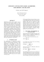
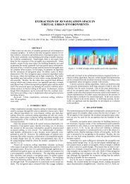
this work, we focus on the detection of two VOC gases: butane and propane.
We use a gas cylinder that consists of 70% butane and 30% propane in our
experiments. Absorption bands of butane and propane are shown in Figure 1.1.
Both of the VOC gases have a peak between 3 and 4 µm bands in the infrared
spectrum. PIR sensor and thermopile sensor have a spectral response of 3~14
µm and 3.26~4.31 µm, respectively. Therefore, we expect to see changes in the
2

output voltages of the sensors when there is a butane or propane leak in the
viewing range of the sensors.
3
(a)
(b)
Figure 1.1 Absorption bands of (a) butane and (b) propane.

For both of the sensors, we design a circuit and obtain a continuous time
analog signal for the sensor outputs. The output is send to a PC and analyzed.
For sensor signal processing, we use Hidden Markov Modeling (HMM). We
first generate a model for each event to be classified, i.e. no-activity, walking
man and VOC gas leak events and determine which model an input signal
belongs to by using a probabilistic approach. In the analysis of the thermopile
sensor data, we also use a periodicity-based approach. The frequency of the
sensor output signal increases with the VOC gas leak. We try to detect VOC
gas leak, by controlling whether the period of an incoming signal is below a
predefined threshold value.
In Chapter 2, we summarize the recent applications of infrared sensors and
conventional gas detectors. We also review the flame detection method
described in [4]. In Chapter 3, we describe the characteristics of a PIR sensor
and a modified PIR sensor circuit designed to obtain a continuous time analog
signal from the PIR sensor output. The methods for VOC gas detection by
using a PIR sensor and a thermopile sensor are presented in Chapters 4 and 5,
respectively. Finally, Chapter 6 concludes this thesis by providing an overall
summary of all results.
4

Chapter 2
Related Work
In recent years, there have been several studies on pyro-electric infrared (PIR)
sensors and several applications of them have been developed, such as intruder
detecting, wisely light controlling, monitoring the flow in traffic, collecting
people’s information [5, 6], etc. PIR sensors are preferred over other sensors
and cameras, mainly because of its faster response time and low-cost.
Additionally, they avoid privacy, extendibility and maintenance issues. Some
of the recent applications of the PIR sensors are described in Section 2.1.
There are several types of detectors commercially available, that use
different detection methods, developed for gas leak. Some important ones can
be summarized as [7, 8]:
- Catalytic detectors,
- Thermal conductivity sensors,
- Semi-conductors, and
- Electrochemical gas sensors.
5

The basic working principles and disadvantages of these sensors are explained
in Section 2.2. In Section 2.3, since we use a similar algorithm based on
Markov models for VOC gas leak detection, we review the flame detection
method by using a pyro-electric (or passive) infrared (PIR) sensor presented by
Cetin et al [4].
2.1 Recent Applications of Pyro-electric Infrared
(PIR) Sensors
In [9], Tsai and Young describe a system for measurement of noncontacted
temperature by monitoring an object’s radiation in the infrared spectrum. They
conduct using a measuring device by passing through a data acquisition and a
long-term observation of the temperature variance of objects on a personal
computer. The measurement mechanism consists of a PIR sensor joined with
an optical chopper and Fresnel lens, where the optical chopper is put between
the sensor and the lens. The proposed system can monitor the temperature of
indoor equipment, especially a power substation with embedded danger, with
an average error rate of 1.21% in the overall range from 40 to 200 °C. It is
stated in [9] that the system provides recognizing the phenomenon of the
temperature rise-rate or the critical temperature point, therefore a possible fire
accident.
There are two approaches for indoor location detection systems: terminal-
based and non-terminal-based method. In terminal-based method, there is a
type of device that should be carried by the resident. However, non-terminal-
based method requires no such device. In [10], Nam Ha et al. present a non-
terminal-based method that uses an array of pyro-electric infrared sensors (PIR
sensors) to detect the location of residents. The PIR sensors are placed on the
6

ceiling and the detection areas of adjacent sensors overlap. Then to locate a
resident, the information collected from multiple sensors are integrated. The
decision for the location of the resident is made due to the strength of the
output analog signals collected from each PIR sensor. In the experimental test
bed in a room of 4 x 4 x 2.5m (width x length x height), the system finds the
location of the residence with an error smaller than 50cm, where the residents
are between 160 and 180cm tall and moving at speeds between 1.5 and 2.5
km/h. Moreover, they prevent pets and other non-human moving objects from
being detected by defining a threshold voltage and using a Fresnel lens, which
allows only human infrared waveforms to pass through it and rejects others.
In [11], Cetin et al. propose a classification method for 5 different human
motion events with one additional “no action” event by using a modified PIR
Sensor. Classified events are tangential walking at 2m, tangential walking at
5m, tangential running at 5m, radial walking from a distance of 5m to the
sensor and radial walking from sensor to a distance of 5m from the sensor.
Classification is done by using Conditional Gaussian Mixture Models
(CGMM) trained for each class. 1-D analog output signal of PIR sensor is fed
into CGMM, logarithmic probabilities of the test signal is calculated according
to each model and the decision is made due to the model yielding highest
probability.
In [12], Lee introduces a method and apparatus for detecting direction and
speed by using a dual PIR sensors in cooperation with a switch controller
employing a counter and a timer. PIR sensors are aligned in a motion plane and
the plurality of the sensors permit speed and direction determinations for
moving IR sources by using the fact that the sensors provide different voltage
outputs depending upon a relative direction of movement of an object. The
switch controller controls the light. When a person enters the room, the switch
turns on the lights and reset the timer. When the timer expires, the lights are
7

turned off. Additionally, the counter counts the number of objects entering or
leaving. If the number of exits equals to number of entrances, the switch
extinguishes the lights. The invention provides an energy conservative switch.
In this thesis, we also deal with a classification problem, but we focus on
the detection of VOC gas leak with a PIR sensor and a thermopile sensor by
using Hidden Markov Modeling and some characteristics of the output signal
of the sensors (i.e., periodicity of the sensor output signal).
2.2 Gas Leak Detectors
Catalytic detector, commonly known as the “pellistor”, used for combustible
gases and is essentially a catalytic microcalorimeter [3]. It has a catalytic
surface constructed around a temperature sensor and a heater to maintain the
catalyst at a sufficiently high temperature for rapid combustion of any
flammable gas molecules present. Temperature measurement and heating
functions are usually combined in a platinum coil which is maintained at
500°C by a current through the wire. When the temperature increases during
combustion, the resistance of the wire changes and the gas concentration is
determined due to these changes [13, 14]. Therefore, catalytic sensor is not
selective and its response depend on the flammable gas concentration and the
rate of diffusion of the flammable gas to the sensor. There must be at least 15%
oxygen (O2) concentration in the environment for the sensor to work.
Moreover, the pellistor can be seriously poisoned by contaminants (e.g., lead,
silicone and certain other gases) in the atmosphere, so that it cannot respond to
a flammable gas and this shortens the lifetime of the sensor [7].
Thermal conductivity (TC) gas detectors operate by comparing the thermal
conductivity of a sample gas with that of a reference gas, which is usually air
8

[7]. Since hydrogen has the highest thermal conductivity of all known gases,
TC sensors are especially used to detect hydrogen [15]. There is a ”cold ” and a
”hot” element in TC sensors and heat is transferred from the hot element to the
cold one via thermal conduction through the investigated gas. The power that is
necessary to heat the hot element is the measure for the thermal conductivity.
TC gas detectors are not very sensitive and can only be used for gases whose
thermal conductivity is significantly different from air.
Semiconductor gas sensors are widely used for detection of inflammable
and certain toxic gases in the air. When a specific gas enters the semiconductor
gas sensor, it reacts with the oxide coating. This causes changes in the
electrical conductivity due to an oxidizing reaction, i.e., a decrease in
resistance between the electrodes and gas concentration is determined by
measuring the resistance [16, 17]. The conductance of the device changes with
the change in the atmospheric composition. Oxygen concentration, temperature
and humidity and exposure to silicone, sulphur compounds may have
significant effect on the sensitivity of the detector. Furthermore, after exposure
to high gas concentrations, the detector may need a recovery time of several
hours [7].
Electrochemical gas sensors are widely used to detect toxic gases. In
general, the electrochemical sensor has two electrodes, “sensing” and
“counter”, divided by an electrolyte thin coat. There is a membrane, through
which the electrolyte is isolated towards the outside and is permeable to gas.
When gas enters the sensor through the membrane by diffusion, oxidation
reaction occurs and this causes an electrical current proportional to gas
concentration. Detection of gas is made due to the current measured between
the electrodes [18]. As catalytic sensors, electrochemical gas sensors
sometimes suffer from poisoning and extreme hot and cold temperatures. In
9

addition, it is stated in [7] that the electrochemical sensors should not be used
in atmospheres containing more than 25% CO2.
Researchers from Siemens Corporate Technology have developed a laser-
supported technique for measuring CO concentration [19]. It works using a
laser diode which emits infrared light with a wavelength of 2.3 micrometers. If
the light beam passes through carbon monoxide, the beam is attenuated at the
absorption wavelength and the gas is detected by the sensor. But, there is no
experimental result and it is only stated that the system can reliably measure
CO at a concentration as low as 10 ppm using an optical path length of 10
centimeters.
The weakness of the conventional detectors is that the gas has to reach the
sensor in order to be detected. Therefore, conventional detectors cannot
provide quick responses in large areas and cannot be utilized in open areas. On
the other hand, PIR and thermopile sensors can be used both in large and open
areas. Since they generate a voltage proportional to the incident infrared
radiation power, it is sufficient for the VOC gas to be in the viewing range of
the sensors. Other advantages of the thermopile and PIR sensors can be
summarized as follows:
- Instantaneous response time,
- no poisoning,
- no need of oxygen, and
- low-cost.
10

2.3 Flame Detection System Based on Wavelet
Analysis of PIR Sensor Signals With An HMM
Decision Mechanism
In [4], a flame detection method with a PIR sensor by using an HMM
decision mechanism is described. There are three types of events to be
classified by using HMMs: a walking person, no-activity and flame. A model
for each class is trained using past data. In this probabilistic approach, the test
signal is classified according to the model for which HMMs produce the
highest probability.
For VOC gas leak detection, we use a similar method to one in [4]. In this
section, we review the flame detection method. We give a brief description of
Hidden Markov Models in Section 2.3.1. The details of the flame detection
procedure is described in Section 2.3.2.
2.3.1 Hidden Markov Models (HMM)
HMMs are commonly used in many real world applications to solve pattern
recognition problems, e.g., speech recognition, gesture recognition. A Markov
process is any process in which the current state depends only on the previous
N states of the sequence [20]. For example, the sequence of a simple set of
traffic lights (red-green-amber-repeat) represents a first order Markov process.
But from a modeling perspective, stochastic processes are more interesting
than deterministic processes. For example, the weather is a stochastic process.
However the states of the model are usually not directly observable. This is
where HMM finds its application. An HMM is a doubly stochastic process in
11

which the underlying states are hidden, and probabilistically related to a
sequence of observed symbols [21]. A simplified example is described in [22]
to understand HMM more. You are in a cave by the ocean and never see
outside. You want to know what the weather is like and the only clue is a piece
of seaweed that you can see from the entrance of the cave. The seaweed can be
dry, dampish or wet depending on the weather. This scenario can be modeled
by an HMM, where the weather is a set of hidden states and the condition of
the seaweed is an observable symbol.
In [4], there are two classes: one represents fire events and the second
represents non-fire events, i.e., background (no activity), walking, running,
hands waving etc. It is stated that the flames of an uncontrolled fire flicker with
a frequency of around 10 Hz. Recently developed fire detection schemes that
are based on video, uses this fact and detects the periodic high-frequency
behavior in moving pixels of flame color. But flame flicker covers a wide-band
range 1 Hz to 13 Hz. Therefore, Markov modeling takes advantage of
producing more robust performance over frequency domain based methods.
2.3.2 Sensor Signal Processing
In [4], a modified PIR sensor circuit is developed to capture a continuous time
analog signal that represents the strength of the received signal in time. The
analog signal is sampled with a sampling frequency of fs=50 Hz. The sampling
frequency is sufficient, because it is above the highest flame flicker frequency
(which is 13 Hz). Having the continuous analog signal, the signal is digitized
by using an analog to digital converter circuit and sent to a PC.
First, a wavelet transform takes place on the sensor output signal. Wavelet
transform provide robustness against sensor signal drift due to temperature
12

variations in the area of interest. Since temperature changes are slow variations
compared to moving objects and flames and wavelet signals are high-pass and
band-pass signals, signals are not affected by the slow variations,
corresponding to temperature variations. The wavelet coefficients for the
output signal, w[k], are obtained after high-pass filtering followed by
decimation. The high pass filter, H(z) has the following transfer function:
1 1 −1
1
H( z) = − ( z + z )
(2.1)
2 4
Having the wavelet coefficients, an HMM based classification is carried
out. Two three-state Markov models are used, one for fire and the other for
walking action for a person. Two threshold values are defined for each model
in the wavelet domain, T1 and T2, where the thresholds are non-negative. Let
the states be S1, S2 and S3 and |w[k]| represent the absolute value of the wavelet
coefficients. If |w[k]| < T1, then state S1; if T1 < |w[k]| < T2, then state S2; if
|w[k]| >T2, then state S3 is attained. In the Markov models defined, S1 represents
no activity case. As long as there is no activity in the viewing range of the PIR
sensor, the system remains in S1.
In the first step of the HMM based analysis, the wavelet coefficient
sequences are divided in windows of 25 samples. Further, the corresponding
state transition sequence is determined for each window. An example state
transition sequence of size 5 may look like
C ={S2, S2, S1, S3, S1}. (2.2)
The wavelet signal captures the high frequency information in the signal.
Therefore, it is expected to see more transitions between states in the case of
fire compared to walking event of a person.
13

The thresholds, T1 and T2 determine the states and the state transition
probabilities of a given signal. Optimum value of the thresholds are defined in
the training step by using a Genetic Algorithm (GA). Having the reference
signals for each class and the threshold values, transition probabilities of the
classes are calculated. The state transition probabilities for a walking person
and fire are estimated from 250 consecutive wavelet coefficients covering a 10
seconds time. Let aij denote the transition probabilities for fire, bij denote the
transition probabilities for a walking person and C denote a state transition
sequence to be tested of size L. To decide which class that C belongs to, two
joint probabilities Pa(C) and Pb(C) (corresponding to fire and walking person
classes, respectively) are calculated:
and
∏ + 1 ∏ i ,
(2.3)
i+
1
P ( C) = p ( C | C ) = a
a a i i C C
i i
∏ + 1 ∏ i ,
(2.4)
i+
1
P ( c) = p ( C | C ) = b
b b i i C C
i i
where i=1, …, L. The state transition sequence C belongs to ‘fire’ class, if
Pa(C)>Pb(C), otherwise it belongs to ‘walking person’ class. The state diagram
and the definitions of the state transitions are presented in Figure 2.1.
14

Figure 2.1: State diagram and the definitions for the state transitions for (a) ‘fire’ and (b)
‘walking person’ classes
During classification, each 50 consecutive wavelet coefficients are
computed from the received PIR sensor signal and fed into ‘fire’ and ‘walking
person’ models. The result of the analysis is monitored as the model yielding
the higher probability.
15

Chapter 3
Properties of PIR Sensor and Analog
Signal Processing
Passive Infrared Sensor (PIR) based system has the detection ability to monitor
large rooms and spaces, because PIR sensors analyze the infrared light
reflected from hot objects to make a decision. Pyro-electric sensors give an
electric response to not the temperature itself, but the rate of change in the
temperature. When there is a hot body motion in the viewing range of the
sensor, the strength of the received signal from the PIR sensor increases.
In Section 3.1, we introduce the characteristics of a PIR sensor. Section 3.2
describes the modified PIR sensor circuit developed in [4], which we also use
for VOC gas detection.
16

3.1 Characteristics of the PIR Device
Pyro-electric detectors are crystal devices. The crystalline material in the PIR
sensor, generates a surface electric charge when it is heated by infrared
radiation. The amount of this charge changes with the amount of radiation
striking the crystalline material. Infrared radiation is absorbed by a coating on
the crystal surface and converted to heat. The heat alters the lattice spacing of
the crystal and causes a charge differential between the surfaces [6, 23]. This
charge differential is measured as an output voltage.
The PIR325 sensor has two sensing elements in connection with a voltage
bucking configuration. Signals caused by vibration, temperature changes and
sunlight are cancelled by this arrangement. When a body passes in front of the
sensor, it will activate the first sensing element and then the second one, as
shown in Figure 3.1. However, other sources will affect both of the elements
simultaneously and be cancelled.
Figure 3.1: A moving body activates each sensing element in turn (taken from [23]).
17

The PIR325 sensor has a spectral response of 3~14 µm. The commercially
available PIR sensors generally have Fresnel lens on them, as shown in Figure
4.1, to change the transmission range of the radiation. The PIR325 sensor has
FL65-type lens on it, which is made of an infrared transmitting material that
has an IR transmission range of 8 to 14 µm, in order to be more sensitive to
radiation of human body. But, many gases that we wish to detect in our
environment exhibit bands of absorption line in the infrared part of the
spectrum, from 2.5 to 15 µm (especially 2.5 to 5 µm). Therefore, in this thesis
the Fresnel lens is demounted and PIR325 sensor is used without a lens to be
able to detect VOC gas leaks.
3.2 Modified PIR Sensor System and Data
Acquisition
Commercial PIR sensor circuits produce binary outputs. To process the sensor
signal, a continuous time analog signal is needed. A circuit is developed for
this aim in [4] and shown in Figure 3.2. The circuit captures a continuous time
analog signal that represents the strength of the received signal in time.
The circuit contains 4 low cost LM324 operational amplifiers (op amps),
U1A, U1B, U1C and U1D. Amplifiers U1A and U1B, have a gain of 100,
together form a two stage amplifier circuit, whereas the op amps U1C and U1D
form a window comparator that responds to signals about 200 millivolts above
and below Vcc/2, where Vcc is 5 V. The two stage amplifier circuit is used to
amplify the very-low amplitude raw output at the 2 nd pin of the PIR sensor. The
amplified output signal of U1B is fed into the comparator structure. The
comparator part of the circuit, outputs a binary signal, either 0 V or 5 V. The
analog output signal is measured at the output of U1B, instead of using the
18

inary output of the original PIR sensor circuit. Then, the analog output is
digitized by using a PIC16F877A-type microcontroller device as an analog to
digital converter and sent to the computer via an RS-232 to USB converter.
Finally, the output signal received from the USB port is read from
HyperTerminal application and saved into a text file to be processed.
Figure 3.2: The circuit diagram of the modified PIR sensor circuit for capturing an analog
signal
For VOC gas detection, the analog signal is sampled with a sampling
frequency of fs=100 Hz, which is sufficiently fast to capture a VOC gas leak.
Typical sampled signal for no activity case using 8 bit quantization is presented
in Figure 3.3. The value of the output signal for no activity case changes
between 100 and 150. The x-axis represents the number of samples and since
the sampling frequency of the output signal is 100 Hz, a time domain analysis
can be obtained by dividing each number in the x-axis by 100. Figure 3.4
shows the PIR output signal due to a walking person and a gas leak event at a
19

Figure 3.3: A typical PIR sensor output sampled at 100 Hz with 8 bit quantization when there
is no activity in its viewing range.
distance of 1 m. In Figure 3.4 (a), there is no activity up to 33 rd second and
there is a walking person in the viewing range of the PIR sensor between
seconds 33-40. There is no activity again up to 87 th second and there is another
walking event. In Figure 3.4 (b), a VOC gas leak at 53 rd second is presented,
after a no activity event. VOC gas leak event actually continues up to the end
of the record, but after some time the observed output signal behaves as it
belongs to no activity event. Because, PIR sensor circuit updates its
background when the same event in its viewing range lasts for some time. In
fact, this is due to the fact that the strength of the signal received from PIR
sensor changes with the motion of a hot body and pyro-electric sensors give an
electric response to a rate of change of temperature rather than temperature
itself.
250
200
150
100
50
PIR output
0
0 2000 4000 6000 8000 10000 12000 14000
number of samples
20

250
200
150
100
50
0
0 20 40 60
seconds
80 100 120
250
200
150
100
50
PIR output for a person walking at 1m
Figure 3.4: PIR sensor output signals recorded at a distance of 1m for (a) a walking person and
21
(a)
PIR output for a VOC gas leak at 1m
0
0 20 40 60
seconds
80 100 120
(b)
(b) for a VOC gas leak. Sampling frequency is 100 Hz.

Chapter 4
Detection of VOC Gas Leak by
Using A Pyro-electric Infrared (PIR)
Sensor
In this chapter, a VOC gas leak detection system based on a pyro-electric
(or passive) infrared sensor is described. Digitized PIR sensor data is analyzed
by using HMMs. There are three events of interest of classification: ‘no-
activity’, ’walking person’ and ’gas leak’ classes. A Markov model for each
class is created and the test signal is classified using the Markov models. The
wavelet coefficients are used as feature parameters by Markov models. Section
4.1 describes the HMM-based decision process of which class a test signal
belongs to. Experimental results are presented in Section 4.2.
22

4.1 Sensor Data Processing
The strength of the PIR sensor output signal increases or decreases due to hot
body actions in its viewing range and the analysis is made by using these
changes. Therefore, any changes in the temperature of the room, where PIR
sensor is placed, affect the analysis. Average temperature changes cause a bias
in the output of the sensor. To remove this bias, wavelet transform is used.
Wavelet transform is a very popular transform and used in analysis, denoising
and compression of signals and images [24].
The procedure to obtain the wavelet coefficients is described in Section
4.1.1. How HMMs are applied on the wavelet domain and the way to decide
which class any test signal belongs to is presented in Section 4.1.2.
4.1.1 Wavelet Transform
Let x[n] be a sampled version of the signal coming out of the PIR sensor and
w[k] be the wavelet coefficients, which are obtained after a subband
decomposition process, followed by a dyadic decimation, where k and n are
integers. The filter bank of a Haar wavelet transform is used in the analysis,
which is the same as a single stage Daubechies wavelet [25]. The lowpass and
the highpass filter coefficients of the filter bank are, respectively:
and
h[ n ] = { 1,1}
(4.1)
g[ n ] = {1, − 1}
(4.2)
23

The Discrete Wavelet Transform (DWT) is computed by successive low
pass and high pass filtering of the discrete time-domain signal as shown in
Figure 4.1. In the figure, the low pass filter is denoted by G0 ,while the high
pass filter is denoted by H0. At each level the high pass filter produces detail
information, d[n], while the low pass filter associated with scaling function
produces coarse approximations, a[n]. In this scheme, wavelet coefficients
w[k], are represented by d4[n]. In this analysis, a four-stage decomposition is
used to obtain the wavelet coefficients. Because the significant changes, which
occur in the case of a VOC gas leak and a walking action of a person, are
visible only at the end of the fourth stage. The wavelet coefficients for the
VOC gas leak in Figure 3.4(b) is shown in Figure 4.2.
Figure 4.1: Four-level wavelet decomposition tree
At each decomposition level, the half band filters produce signals that span
only half the frequency band. This doubles the frequency resolution and
decimation by 2 halves the time resolution. Therefore, while the half band low
24

pass filtering removes the half of the frequencies and so halves the resolution,
the decimation by 2 doubles the scale.
While each 100 samples correspond to 1 second in the original data, in
wavelet domain each 100 samples correspond to 16 seconds.
60
40
20
0
-20
-40
-60
-80
0 100 200 300 400 500 600 700
number of samples
Figure 4.2: Wavelet coefficients of the PIR sensor output signal recorded at a distance of 1m
for the VOC gas leak (shown in Figure 4.4(b))
4.1.2 Hidden Markov Modeling
Wavelet coefficients of the gas leak at 1m
Once the wavelet coefficients are obtained with the procedure described in
Section 4.1.1, an HMM based classification, similar to one in [4], is carried out
for VOC gas leak detection. There are three types of event to be classified: a
walking person, a gas leak and a no-activity event. Two three-state Markov
25

models are used to model a VOC gas leak and a walking person. In the training
step, two threshold values are defined in the wavelet domain for each model, T1
and T2, where T1 is negative and T2 is positive. The same threshold values are
used in each model. Let the three states be S0, S1 and S2. States of the wavelet
coefficients are defined according to the algorithm implemented as follows:
if ( w(k) < T1 )
then state S0,
else if (T1 < w(k) < T2 )
else
end
then state S1,
state S2 is attained accordingly.
Figure 4.3: The algorithm for state definitions of the wavelet coefficients
Thresholds are defined such that the wavelet coefficients of the no-activity
event remain in state S1. The system is in state S1 as long as there is not any
significant activity in the viewing range of the PIR sensor. Therefore, although
there are three events to be classified, only two Markov models are used, one
for a walking person and the other for a gas leak. No-activity event is detected
by controlling whether the system remains in S1 or not.
Once thresholds and states are defined, the next step while applying
HMMs is to find the state transition sequences for predetermined reference
signals of a VOC gas leak and a walking person. Let r C be the state sequence
of a reference signal. An example state sequence of size 7 may look like
26

C =( S0 S0 S1 S2 S2 S1 S0) (4.3)
Equation (4.3) shows that the first and the second wavelet coefficients of the
reference signal are below the threshold T1, the third coefficient is between T1
and T2 and so on. The state sequence is generated from the related part of the
signal, i.e. over the part that the VOC gas leak starts and ends for the ’gas leak’
class and the part when there is a walking person in the viewing range of the
sensor for ‘walking person’ class. Let aij and bij be the number of transitions
from state i to j in the state sequences of the reference signals for the ‘gas leak’
and the ‘walking person’ classes respectively and they can be defined as:
a=(a00 a01 a02 a10 a11 a12 a20 a21 a22) (4.4)
b=(b00 b01 b02 b10 b11 b12 b20 b21 b22) (4.5)
where a00 and b00 denote the number of transitions from state S0 to S0, a01 and
b01 denotes the number of transitions from state S0 to S1 and so on. States and
the transitions are demonstrated in Figure 4.4.
Having determined the number of transitions between the states for each
reference signals, the probabilities for each transition to occur are computed.
Let the lengths of the reference signals for ‘gas leak’ and ‘walking person’
classes be L1 and L2, respectively. Then the probability for each transition to
occur is:
and
pa (i,j) =
pb (i,j) =
27
1
L ai j (4.6)
2
1
1
L bij (4.7)

for the ‘gas leak’ and ‘walking person’ classes respectively, where pa (i,j)
denotes the probability of moving from state i to state j. For the training of the
HMMs, the state transition probabilities are estimated from 50 consecutive
wavelet coefficients covering a time frame of 8 seconds. Training step ends up
by obtaining the probabilities for each transition.
Figure 4.4: State transition definitions for (a) ‘VOC gas leak’ and (b) ‘walking person’ classes
In the classification process of the classes with HMMs, we only deal with
the VOC gas leak and walking person events. Since the system remains in state
S1 when there is no activity, the 5 th element of the state transition probability
sequence of the no-activity class, p(1,1), is very close to 1 and others are very
close to 0. Consequently, no-activity event is detected by first defining a
threshold value close to 1 and controlling whether p(1,1) of the test signal state
sequence is above this threshold, without using any extra model.
To decide the class affiliation of a test signal, state vector and accordingly
the number of transitions of the signal are generated first. Let C be the state
28

sequence of the test signal and tij be the number of transitions from i-th state to
j-th state. Then the probabilities for the state sequence C of belonging to ‘gas
leak’ and ’walking person’ classes are, respectively:
and
a
L
∏ a i+ 1 i
2 2
∏∏ a
t
(4.8)
i= 1 i= 0 j=
0
( ) ( | ) ( ( , )) ij
P C = p C C = p i j
b
L
∏ b i+ 1 i
2 2
∏∏ b
t
(4.9)
i= 1 i= 0 j=
0
( ) ( | ) ( ( , )) ij
P C = p C C = p i j
where L is the length of the state sequence C of the test signal.
During the classification phase, the state sequence of the test signal C is
divided into windows of length 25 and each window is fed into ‘gas leak’ and
‘walking person’ models. The model yielding the highest probability is
determined and monitored at the end of each 4 seconds period, as the result of
the analysis of PIR sensor data. To minimize the complexity of operation
during classification, we use equations (4.10) and (4.11) to determine the
probabilities, instead of (4.8) and (4.9). Figure 4.5 describes the algorithm
implemented to decide the result.
2 2
P ( C)' = ∑∑ t log ( p ( i, j))
(4.10)
a ij 10 a
i= 0 j=
0
2 2
P ( C)' = ∑∑ t log ( p ( i, j))
(4.11)
b ij 10 b
i= 0 j=
0
29

if P ( C ) > P ( C )
else
end
a b
then the window affiliates to the ‘gas leak’ class
the window affiliates to the ‘walking person’ class
if p test (1,1) > 0 .8
end
the window affiliates to the ‘no-activity’ class
Figure 4.5: The algorithm to decide the class affiliation of a window of the test state sequence
C
As an alternative way, we try two two-state Markov models to represent
‘VOC gas leak’ and ‘walking person’ models. Since there are two states, only
one threshold, T, is sufficient and it is defined as 2σ and 3 σ , where σ is the
standard deviation of the sensor output signal for no-activity event. Figure 4.6
shows the two-state Markov models and the state definitions. If w(k) < T, then
S0 is attained, otherwise S1 is attained. Greater than 90% of the wavelet
coefficients of the signal for no-activity event remain is state S0. Therefore, the
probability of the system to remain in S0 is greater than 0.9 and a no-activity
event can be classified by controlling this probability without generating an
extra Markov model.
30

When T= 2 σ, the system triggers an alarm at each time there is a walking
person or waving arm movements and when T= 3 σ, all the gas leaks are
considered as a walking person event. When threshold is defined between 2σ
and 3 σ , the system can detect some of the gas leaks but, it may analyze a
walking person event as a gas leak. As a result, three-state Markov models
produce better results than the two-state models.
Figure 4.6: Two state Markov models for (a) ‘VOC gas leak’ and (b) ‘walking person’ classes
4.2 Experimental Results
The analog output signal is sampled with a sampling frequency of 100 Hz and
quantized at 8 bits. Analysis and classification methods are implemented with
MATLAB running on a PC. Digitized output signal is fed to the PC via RS-232
serial port.
The detection range of a PIR sensor based system is 5 meters, but in our
experiments we record VOC gas leak and walking person sequences at a
distance of up to 3 meters. Since we use the PIR sensor without the Fresnel
lens on it, after 3 meters the strength of the PIR output signal decreases and the
sensor is not able to response to the changes.
31

For the VOC gas leak records, we use a bottled gas which contains a
mixture of butane and propane gases, in ratios %70 and %30 respectively and
three types of experiments are hold:
- We record the VOC gas leak when it is very close and at a distance
of 1m and 3 meters to the sensor. We first start the VOC gas leak, leave
the viewing range of the sensor, wait until the response to a walking
person disappears and then start recording.
- We use 1m-length pipe between the sensor and the bottled gas. We
start recording the background and then start the VOC gas leak while
recording continues.
- We first start recording the background and then start the VOC gas
leak without entering the viewing range of the sensor.
The first type of experiments are uncontrolled, while the others are controlled.
For walking person sequences, we record a person walking in the viewing
range of the PIR sensor on a straight line which is tangent to a circle with a
radius of 1m, 2 and 3 meters and the sensor being at the center. We also record
waving arm movements at distances of 1m, 2 and 3 meters to the sensor.
Moreover, we record the response of the PIR sensor to air coming out of a
hairdryer to test whether it will be considered as a gas leak or not. The second
setup described above used in hairdryer experiments. PIR sensor output for
hairdryer is shown in Figure 4.7.
32

250
200
150
100
50
Figure 4.7: PIR sensor response to hairdryer at a distance of 1m from the sensor
In the HMM-based analysis of the PIR sensor output signal, we use the
same model to test each test sequence. We also use the same threshold values,
( T1 T2
0
0 2000 4000 6000 8000 10000 12000 14000 16000 18000
number of samples
= − 10, = + 10 ) to produce the reference transition probabilities and the
transition numbers for the test signals. The state sequence is divided into
windows of lengths 25, each covering a time frame of 4 seconds. At the end of
each time frame, the result of the analysis is monitored and hold. If two
consequent frames are analyzed as gas leak, we trigger an alarm. Moreover, if
the probability of a transition from 1 S to 1 S to occur is greater than 0.8, we
decide there is no-activity.
PIR sensor response to hairdryer
The response to a hairdryer, shown in Figure 4.7, is similar to the response
to VOC gas leak and a walking man, but the oscillations do not die down. In
the case of a VOC gas leak, PIR sensor updates its background after some time
33

and the sensor output signal behaves as there is no activity even if there is a gas
leak. Therefore, if the analysis of 10 consecutive windows are concluded in
VOC gas leak or walking man, then the alarm is turned on. The results for the
HMM analysis are presented in Table 4.1.
No. of test sequences
34
No. of
False
Alarms
No. of
Missed
Leaks
No. of
Alarms
Gas leak test sequences 32 - 2 30
Non-gas test sequences 50 5 - 5
Table 4.1 Classification results for 32 VOC gas leak and 50 non-gas test sequences. The
system triggers an alarm when a VOC gas leak is detected in the viewing range of the PIR
sensor.
Our method successfully detects VOC gas leak for 30 of the 32 gas leak
test sequences. The two missed leaks belong to leaks that are at a distance
greater than 3 meters to the sensor. The strength of the output signal of the PIR
sensor decreases for the leaks far away from the sensor and they are analyzed
as a no-activity event. Our system triggers a false alarm for 5of 50 non-gas test
sequences. Three of them belong to the walking person and two of them belong
to the waving arm movement experiments. If a person is at a distance of up to
1m, there is no problem. But, when the person is far away, the strength of the
sensor output signal decreases, as a result walking event may be confused as
gas leak.

Chapter 5
Detection of VOC Gas Leak by
Using A Thermopile Sensor
In this chapter, a thermopile sensor based VOC gas leak detection method is
described. Thermopile sensor output signal changes due to the absorption of
infrared radiation in its viewing range. A circuit is designed to process the
sensor signal in PC. Sensor output signal is analyzed by using HMMs in
wavelet domain and using the periodicity of the signal and determined which
class, ‘gas leak’ or ‘no-activity’, it belongs to.
In Section 5.1, we introduce the properties of the thermopile device.
Section 5.2 describes the circuit designed for sending the sensor data to PC. In
Section 5.3, we review the method in [26], which we use to detect the periodic
behavior of a signal. Sensor output signal analysis is made in Sections 5.4 and
5.5 and the experimental results are presented in Section 5.6.
35

5.1 Characteristics of the Thermopile Sensor
A thermopile is an electronic device that converts thermal energy into electrical
energy. It measures the increase in temperature caused by the absorption of
radiation [27]. It is composed of a serially-interconnected array of
thermocouples, each of which consists of two dissimilar materials with a large
thermoelectric power and opposite polarities. The thermocouples are placed
across the hot and cold regions of a structure. The hot junctions are thermally
isolated from the cold junctions. To provide effective heat sink, the cold
junctions are placed on the silicon substrate. In the hot region of the sensor a
black infrared radiation absorbing coating is applied. This absorbs the radiation
and transduces it into heat. The heat causes temperature differences across the
thermopile, which thus gives an output according to the intensity of the
incident infrared light [28].
Heimann HIS A21 F4.26 4PIN type thermopile sensor has a spectral
response of 3.26-4.31 µm [29]. Gases that have a characteristic absorption peak
in this infrared band are sensed by the sensor. When infrared radiation passes
through the gas, light energy is absorbed by its molecules. The base equation
for gas concentration measurement in the infrared way is the Lambert-Beer
law [30]:
I I exp( K C L )
= − (5.1)
0
where I0 and I, denote the light intensity of infrared parallel light before and
after passing the gas to be measured respectively; K denotes the absorption
coefficient of gas, C denotes the gas concentration and L denotes the measuring
distance.
The thermopile sensor has two output channels. One is the active channel
and the other is the reference channel. Output signal of the active channel is
36

proportional to the light intensity and the gas concentration, whereas the
reference channel output does not relate to the gas to be measured and is
proportional to the light intensity too. Both output signals are proportional to
light intensity and K and L are fixed for a sensor. Therefore, two scale factors,
K1 and K2, can be estimated for two channels and consequently, the output
signals can be defined as:
and
U K I ex p ( K C L )
= − , (5.2)
1 1 0
U 2 = K 2 I
(5.3)
0
for the active channel and the reference channel, respectively. The peak-to-
peak voltage of the active channel lessens with the light energy absorbed by the
gas molecules.
5.2 Modified Thermopile Sensor System and Data
Acquisition
The active channel of the thermopile sensor is used for sensor signal
processing. The circuit shown in Figure 5.1 is constructed to obtain a
continuous time analog signal. It contains two LM324 operational amplifiers,
U1A and U1B. U1A is used to amplify the very-low amplitude output at the 4 th
pin of the thermopile sensor and the output is read from the unity gain
amplifier, U1B. R1-C1 couple is used to filter the noise. R3 resistor limits the
current which must be in 1-2 mA range. The sensor pins are configured as in
Table 5.1.
37

Pin No. Symbol Description
1 VDD Positive supply voltage (+5V)
2 VSS Ground (0V)
3 AOR Analog temperature reference output voltage
4 AOT Analog sensor output voltage
Table 5.1: Pin / Device configuration for the thermopile sensor
Figure 5.1: The circuit diagram of the modified thermopile sensor circuit for capturing an
analog signal
The analog output is digitized by using a PIC16F877A-type
microcontroller device and sent to the computer via an RS-232 to USB
38

converter. Then, the output signal received from the USB port is read from
HyperTerminal application and saved to be processed.
The continuous time analog signal is sampled with a sampling frequency, fs, of
100 Hz and quantized at 8 bits. Typical sampled signals for no-activity case
and gas leak event are shown in Figure 5.2. The x-axis in the figures represents
the number of samples recorded. Each 100 samples correspond to 1 second.
The VOC gas leak, shown in Figure 5.2 (b), is very close to the thermopile
sensor (at a distance of 15-20 cm). The most significant property of the sensor
output signal is its periodicity. In addition, periods of the signals for no-activity
case and gas leak event are different. Frequency of the signal increases with the
presence of VOC gas leak in the viewing range of the thermopile sensor.
94
93.5
93
92.5
92
91.5
91
90.5
Sensor output for no-activity case
90
0 500 1000 1500 2000 2500 3000 3500 4000
number of samples
(a)
39

(b)
Figure 5.2: Thermopile sensor output signal for (a) no-activity and (b) VOC gas leak. Sampling
frequency is 100 Hz.
5.3 Analysis of Periodic Nature in Signals
In the analysis of the output signal received from the thermopile sensor,
one can observe the increase in the frequency of the output signal when there is
a VOC gas leak in the viewing range of the thermopile sensor. In Section 5.4,
we develop a method for VOC gas leak detection, by using the periods of the
sensor output signals for no-activity and gas leak event. We will use the
method developed for images in [26], to detect periodic behavior in 1-D
signals.
95
94.5
94
93.5
93
92.5
92
91.5
91
90.5
Sensor output for gas leak
90
0 500 1000 1500
number of samples
2000 2500 3000
Cutler and Davis [26] describe a technique that detects periodic motion in
images. Similarity between images is used to detect and analyze periodicity.
40

They first segment moving objects from the background and compute the
object’s self-similarity. The self-similarity metric is periodic for periodic
motion and is analyzed in Fourier domain for detection and characterization of
periodicity.
In [26], it is assumed that the camera is static, the size and the orientation
of the objects of interest do not change apparently during several periods and
the frame rate is sufficient to capture the periodic motion. In segmentation of
the moving object, it is suggested to first compute a background and then
subtract it from the current image. Background is computed by taking the 1-D
median for each pixel over the previous N frames (N is between 50 and 200).
For subtraction of the background B with the current image I, the following
color similarity metric,
D( x, y) = ∑ | Ic ( x, y) − Bc ( x, y)
|
(5.4)
C∈{ R, G, B
}
is used. The foreground threshold is set to the value K σ , where K is a constant
and σ is the average standard deviation of the white noise in the video system
for the RGB color channels (σ � 3 and K is typically 10). Having the
foreground, moving objects are tracked by using a template-based tracker.
To detect periodicity, segmented object is first aligned using the object’s
centroid and resized by using a Mitchell filter to have the same dimensions.
Further, the self-similarity of the object O is computed at times t1 and t2 and
the image similarity metric is:
S( t1, t2) = min ∑ | Ot ( x+ dx, y+ dy) −Ot
( x, y)|
(5.5)
| dx, dy| ≤r
( x, y) ∈B
Ot1 1 2
41

is search radius and is used to account for any errors in tracking. It is stated
that S is periodic for periodic motions and a similarity plot should be
symmetric. In addition, there will be a dark line on the main diagonal and
periodic motions will also have dark lines or curves parallel to the diagonal. To
determine if the object has a periodic behavior, 1-D power spectrum of S(t1, t2)
is estimated for a fixed t1 and all values of t2. In [26], it is indicated that a
periodic motion will show up as peaks in the spectra at the motion’s
fundamental frequencies and a peak (or peaks) is significant at frequency fp if,
P(fp) > µp + Kσ p,
where P(fp) is the power estimate, K is a threshold value
(typically 3), µp is the mean and σ p is the standard deviation of P .
To illustrate the analysis of periodic motion, Figure 5.3 is given in [26]. A
test sequence is obtained from a walking person. Figure 5.3 (a) is the first
image of a 100 image walking sequence. In similarity plot, Figure 5.3 (b), there
is a dark line on the main diagonal and there are also dark lines parallel to the
diagonal which represent periodic motions. Figure 5.3 (c) shows the power
spectrum of similarity. There are two peaks showing the period, one for the
swinging arm and the other for legs.
42
(a)

(b)
(c)
Figure 5.3: (a) First image of the walking sequence. (b) Walking sequence similarity plot. (c)
Average power spectrum of all columns.
43

5.4 Period-based Analysis of the Sensor Data
The period-based analysis of the thermopile sensor output signal uses the fact
that the signal is periodic and the period is different for ‘no-activity’ and ’gas
leak’ classes. First, whether the output signal is periodic or not is determined
by modifying the method in [26] to 1-D signal case and then the period of each
member of each class is found. Section 5.4.1 describes the process to determine
whether the signal is periodic or not.
5.4.1 Detection of Periodicity
To determine whether the thermopile output signal is periodic or not, the
procedure described in [26] is used with appropriate modifications. A camera is
used in [26] and the technique for periodicity detection is introduced
accordingly, but the thermopile sensor can be visualized as a single-pixel
camera and therefore the periodicity calculation for video image can also be
used for the thermopile sensor. A similarity plot and 1-D power spectrum of
the output signal is estimated. For periodic motions similarity plot is periodic
and a periodic motion shows up as a significant peak in the spectra at a
frequency fp if P(fp) > µp + Kσ p,
where P(fp) is the power estimate, K is a
threshold value and equals to 3, µp is the mean and σpis the standard deviation
of P.
The output signal is smoothed first by using a sequence of moving average
filters. Let the output signal of the sensor be x[n] and y[n] be the smoothed
signal. y[n] by using a span of 5 is described as follows [31]:
44

1
y[ n] = ( x[ n− 2] + x[ n− 1] + x[ n] + x[ n+ 1] + x[ n+
2]) (5.6)
5
Figure 5.4 (a) shows the smoothed sensor signal output for a VOC gas leak, by
using a sequence of moving average filters.
Then the difference matrix m of y[n] of length l is obtained by using
equation (5.2). Consequently, the difference matrix has a size l x l. The
smoothed output signal y[n] and the similarity plot for the VOC gas leak shown
in Figure 5.2 (b) is presented in Figure 5.4. Similarity plot is symmetric and
there is a dark line on the main diagonal with the dark curves parallel to it,
which are observed when the signal is periodic.
⎡ 0 y(1) − y(2) y(1) − y(3) ... y(1) − y( l)
⎤
⎢
y(2) y(1) 0 y(2) y(3) ... y(2) y( l)
⎥
⎢
− − −
⎥
⎢ y(3) − y(1) y(3) − y(2) 0 ... y(3) − y( l)
⎥
m = ⎢ ⎥
⎢ . . . . . ⎥
⎢ . . . . . ⎥
⎢ ⎥
⎣ y( l) − y(1) y( l) − y(2) y( l) − y(3)
... 0 ⎦
The difference matrix can also be denoted as:
m [ c c c ... c ]
1 2 3
45
l
(5.7)
= (5.8)
Let i m denote the mean of the column i . i m ’s are subtracted from i c ’s and
absolute value of the difference vector with updated c ’s is taken after a Fast
i
Fourier Transform (FFT). Average power spectrum is obtained by taking the
mean of all rows in m and is shown in Figure 5.5. The signal has significant
peaks where P(f) > µp + K σ p.
Therefore, it is concluded that the sensor output

signal is periodic and a period-based analysis can be carried out for VOC gas
detection.
93.5
93
92.5
92
91.5
91
90.5
0 500 1000 1500
number of samples
2000 2500 3000
(a)
(b)
Figure 5.4: (a) Smoothed output signal using a sequence of moving average filters (b)
similarity plot of the VOC gas leak.
smoothed sensor output signal for gas leak
46

Power
45
40
35
30
25
20
15
10
5
Spectra Power of Similarity
0
0 50 100 150
Frequency(Hz)
Figure 5.5: Average power spectrum of all columns
5.4.2 Methods of Finding the Period of a Signal
The period of the sensor output signal can be found from the original data by
first smoothing the signal and taking the mean of the distances between
maxima or minima points, also known as extremas. Extremas are detected as
follows: First the difference between subsequent elements are computed and
hold in a difference vector. The elements in the difference vector are changed
with ‘1’s if they are positive, otherwise with ‘0’s. A positive value means
positive slope and a negative value means negative slope. Afterwards, the
differences between subsequent elements in the updated difference vector are
computed. Let i and j be the index of the values -1 and +1 in the last difference
vector, respectively. Then i+1 is the index of the maxima point and j+1 is the
47
Mean
Mean+3*SD
Power

index of the minima point. In the case of flat peaks, which are not common in
the sensor output signal, the middle element in the flat peak is detected as
extrema. The first and the last detected maxima or minima points are not taken
into account in the analysis, because they are always considered as extrema due
to the algorithm implemented, however may be not. In this section, alternative
methods to find the period are introduced: Average Power Spectrum Method,
Average Magnitude Difference Function Method (AMDF), Auto-covariance
Method and Co-difference Method.
Average Power Spectrum Method
In this method, the same procedure in Section 5.3 is followed and the average
power spectrum of all columns is obtained. Then, the index of the peak that has
the maximum value is found. The period is detected by dividing the length of
the transformed difference vector by this index.
In the following methods, once the functions are obtained, maxima and
minima points are detected and the period is determined accordingly. Functions
have the same periods with the original signals.
Average Magnitude Difference Function (AMDF) Method
Average magnitude difference function is a variation on autocorrelation
analysis. Instead of correlating the input signal, it forms a difference signal
between the original and delayed signal and the absolute magnitude of the
difference is taken at each delay [32]. AMDF is defined as:
48

N−1
1
Ψ y(
n) = ∑ | y( k) − y( n+ k)
|
(5.9)
N
k=
0
where N is the length of the signal y(n). Ψ ( n)
is smoothed by a sequence of
moving average filters and the period is determined after the detection of the
extremas followed by averaging the distances between each maxima or minima
points in terms of number of samples. AMDF of the VOC gas leak in Figure
5.2 (b) is shown in Figure 5.6.
2.5
2
1.5
1
0.5
AMDF for the gas leak
0
0 500 1000 1500
samples
2000 2500 3000
Figure 5.6: Average magnitude difference function for the VOC gas leak
49

Autocorrelation Method
Autocorrelation is the cross-correlation of a signal with itself [6] and described
by:
N−1
1
Φ [ n] = ∑ ( y[ k] − m )( y[ n + k] − m )
(5.10)
y y y
N k=
0
where N is the length and y m is the mean of the signal y[n]. Maximum
similarity occurs when the time shifting is zero and another maximum should
occur when the time shifting of the signal corresponds to the fundamental
period. Therefore the index of the second maximum is the period of the signal.
Autocorrelation function of the VOC gas leak in Figure 5.2 (b) is shown in
Figure 5.7.
1.4
1.2
1
0.8
0.6
0.4
0.2
0
-0.2
-0.4
Autocorrelation function for the gas leak
-0.6
0 500 1000 1500
samples
2000 2500 3000
Figure 5.7: Autocorrelation function for the VOC gas leak with marked extrema point
50

Co-difference Method
A novel technique, Co-difference Method, is described to find the period of a
signal. Co-difference function is defined as:
N−1
1
Γ [ n] = ∑ ( y[ k] −m ) ⊗ ( y[ n+ k] −m
)
(5.11)
y y y
N k=
0
where N is the length and y m is the mean of the signal y[n] and the operator is
defined as follows:
A ⊗ B = sgn( AB )(| A | + | B |) , (5.12)
for A, B ∈ ℜ . Co-difference function of the VOC gas leak in Figure 5.2 (b) is
shown in Figure 5.8. The period of the input signal is equal to the period of its
co-difference function and found by using the extrema point analysis.
1.2
1
0.8
0.6
0.4
0.2
0
-0.2
-0.4
Co-difference function of the gas leak
-0.6
0 500 1000 1500
number of samples
2000 2500 3000
Figure 5.8: Co-difference function of the VOC gas leak with marked extrema points
51

5.5 HMM-based Analysis of the Sensor Data
The HMM-based analysis is carried out in the wavelet domain. Because,
wavelet sub-signals of a waveform are not affected by the slow variations in
the environment, which is desired to be so. Let x[n] be a sampled version of the
signal coming out of the PIR sensor and w[k] be the wavelet coefficients.
Wavelets are obtained after an high pass filtering followed by a dyadic
decimation as shown in Figure 5.10. Wavelets of the VOC gas leak are shown
in Figure 5.9. While each 100 samples correspond to 1 second in Figure 5.2
(b), in the wavelet domain each 100 samples correspond to 2 seconds, because
of downsampling the high-pass filtered signal by a factor of 2.
Figure 5.9: Single-stage wavelet filter bank
While applying HMMs on the sensor signal in the wavelet domain, a
similar procedure is used with the one in Section 4.3.2. In this case there are
two types of events to be classified: no-activity and gas leak. Two threshold
values, T1 and T2, are defined such that T1 is negative and T2 is positive and
they are symmetric with respect to the x-axis. Wavelet coefficients of the no-
activity event remains between T1 and T2. Then the states are introduced
accordingly. If w[n] < T1, then state S0; if T1< w[n] < T2, then state S1 and if
w[n]>T2, then state S2 is attained. In no-activity case, the system remains in
state S1.
52

The next step is to compute state transition sequences for predetermined
reference signals. Since each reference signal contains one type of event, the
whole signal is of interest in the training step. Let aij and bij be the number of
transitions from state i to j in the state sequences of the reference signals for the
‘gas leak’ and the ‘no-activity’ classes respectively and they can be defined as:
1.5
0.5
-0.5
-1.5
x 10-4
wavelets
2
1
0
-1
a=(a00 a01 a02 a10 a11 a12 a20 a21 a22) (5.13)
b=(b00 b01 b02 b10 b11 b12 b20 b21 b22) (5.14)
for the gas leak
-2
0 500 1000 1500
samples
Figure 5.10: Wavelet coefficients of the VOC gas leak in Figure 5.2 (b)
53

The state diagrams are shown in Figure 4.7. Let the lengths of the
reference signals for ‘gas leak’ and ‘no-activity’ classes be L1 and L2,
respectively. Then the reference probabilities for each transition to occur is:
and
pa (i,j) =
pb (i,j) =
54
1
L ai j (5.15)
1
1
L bij (5.16)
for the ‘gas leak’ and ‘no-activity’ classes respectively. For the training of the
HMMs, the state transition probabilities are estimated from the wavelet
coefficients covering a time frame of 25 seconds. Let tij be the number of
transitions from state i to j for the test signal. Then the probabilities for the
state sequence C of belonging to ‘gas leak’ and ’no-activity’ classes are,
respectively:
and
2 2
a ij 10 a
i= 0 j=
0
2
P ( C) = ∑∑ t log ( p ( i, j))
(5.17)
2 2
P ( C) = ∑∑ t log ( p ( i, j))
(5.18)
b ij 10 b
i= 0 j=
0
where L is the length of the state sequence C of the test signal. The state
sequence C is divided into windows of length 150 and each window is fed into
each model. The model that yields the highest probability is determined as the
result of the analysis of that window. Each window corresponds to 3 seconds,
therefore the result is monitored at each 3 seconds.

5.6 Experimental Results
The sensor output signal is sampled at 100 Hz and quantized at 8 bits. Analysis
of the signal is made in MATLAB running on a PC. Digitized output signal is
fed to the PC via RS-232 serial port.
We record the VOC gas leak many times at a distance of 15-20 cm away
from the sensor. We use a bottled gas, which contains a mixture of butane and
propane gases, in ratios %70 and %30 respectively. Experiments are hold in
three different rooms and we record only one type of event at each experiment,
i.e., no-activity or VOC gas-leak.
In the period-base analysis of the sensor output signal, the period of each
test signal is computed. It is noted that the frequency of the signal increases
with the VOC gas leak. In other words, the periods of the signals that belong to
‘no-activity’ class are greater than the ones of ‘gas leak’ class in general. The
classification of events are made by defining a threshold. If the period of the
input signal is below that threshold, then we end up with a gas leak, otherwise
no-activity in the viewing range of the sensor. 24 experiments are made in
total, 8 for each room, and the periods of the sensor output signal that are
computed with different methods are presented in Table 5.2. Since the output
of the thermopile detector is varying according to the ambient temperature, we
define different thresholds for each room. We trigger an alarm if the period of
the test signal is below that threshold. VOC gas-leak is successfully detected
for all test sequences with an acceptable number of false alarms when there is
no-activity. Table 5.3 summarizes the results for 24 test sequences for each
method. Except AMDF, the other three methods for finding period have only
one false alarm and that occurs as a response to a no-activity test sequence.
55

Room#1
Room#2
Room#3
no-activity#1
no-activity#2
no-activity#3
no-activity#4
gas leak#1
gas leak#2
gas leak#3
gas leak#4
no-activity#1
no-activity#2
no-activity#3
no-activity#4
gas leak#1
gas leak#2
gas leak#3
gas leak#4
no-activity#1
no-activity#2
no-activity#3
no-activity#4
gas leak#1
gas leak#2
gas leak#3
gas leak#4
Spectral
domain
method
[26]
AMDF
56
Auto-
correlation
method
Co-
difference
method
500 593 628 637
735 880 853 845,5
501,66 599,5 436 574,66
527,65 553,43 641 ,2 633,3
333,28 301,4 348,9 364,57
428,57 524,25 519,33 528
276 323,87 324 316,16
269,09 256,90 205,09 230,63
614,66 501,57 444,41 569,64
648,18 629 498,73 590,3
1365 802,4 808,55 793,6
560 592,71 560,43 571,66
605 427,83 326,37 476
565 529,28 517,8 542,8
387,5 363,71 290,85 423,4
483,33 412,39 415 438,4
310,72 322,1 271,34 249,5
437,78 490,17 480,33 493,33
300,79 272,1 251,23 348,3
339,44 356,6 359,53 370,07
208,57 219,61 236,294 323,46
257,4 201,5 280 227,5
267,83 253,68 240,044 256,73
247,27 233,22 269,125 230
Table 5.2: Periods of the test sequences, that belong to no-activity and VOC gas leak classes,
computed by different methods

Room#1
Room#2
Spectral domain
method [26]
AMDF
No. of sequences
57
No. of False
Alarms
No. of
Alarms
gas-leak test sequences 4 0 4
no-activity test sequences 4 0 0
gas-leak test sequences 4 0 4
no-activity test sequences 4 0 0
gas-leak test sequences 4 0 4
Auto-correlation no-activity test sequences 4 1 1
Co-difference
Spectral domain
method [26]
AMDF
gas-leak test sequences 4 0 4
no-activity test sequences 4 0 0
gas-leak test sequences 4 0 4
no-activity test sequences 4 1 1
gas-leak test sequences 4 0 4
no-activity test sequences 4 1 1
gas-leak test sequences 4 0 0
Auto-correlation no-activity test sequences 4 2 2
Co-difference
gas-leak test sequences 4 0 4
no-activity test sequences 4 0 0
Table 5.3: Results for 12 VOC gas leak and 12 no-activity test sequences for different methods.
The system triggers an alarm when VOC gas leak is detected.

Room#3
58
No. of
Sequences
No. of False
Alarms
No. of
Alarms
Spectral
domain method
gas-leak test sequences 4 0 4
[26] no-activity test sequences 4 0 0
AMDF
gas-leak test sequences 4 0 4
no-activity test sequences 4 0 0
gas-leak test sequences 4 0 4
Autocorrelation no-activity test sequences 4 2 2
Co-difference
gas-leak test sequences 4 0 4
no-activity test sequences 4 1 1
Table 5.3: Results for 12 VOC gas leak and 12 no-activity test sequences for different methods.
The system triggers an alarm when VOC gas leak is detected.
In the HMM-based analysis, we test each sequence by a predetermined
model for each room and the same thresholds,
T1 0 .5 x1
0
− 4
= − and − 4
T 2 = 0 .5 x1
0
are used both for training and the test sequences. Each test sequence is divided
into windows of length 150, covering a 3 seconds-time frame. The result of the
analysis of each window is hold. If the result of the analysis of two consequent
frames is both the gas leak, then the system triggers an alarm. Our method
successfully detect the VOC gas leak in room 1. In rooms 2 and 3, VOC gas
leak is successfully detected also, but there is a false alarm when there is no
activity in the viewing range of the thermopile sensor. Table 5.4 presents the
results of the HMM-based analysis of the sensor output.
,

Room#1
Room#2
Room#3
No. of Sequences No. of False Alarms No. of Alarms
Gas Test Sequences 4 0 4
No-activity Sequences 4 0 0
Gas Test Sequences 4 0 4
No-activity Sequences 4 1 1
Gas Test Sequences 4 0 4
No-activity Sequences 4 1 1
Table 5.4: Classification results of the HMM-based analysis for 12 VOC gas leak and 12
no-activity test sequences
59

Chapter 6
Conclusion and Future Work
In this study, we proposed and implemented novel and cost efficient methods
for VOC gas detection by using a passive infrared sensor and a thermopile
sensor. We used the fact that the sensors have spectral responses in the infrared
part of the spectrum intersecting with the absorption bands of butane and
propane gases. Gases spread out gradually, whereas the IR radiation
propagation is very rapid. Therefore, unlike conventional detectors, infrared
and thermopile detectors have fast response time. For example, a ME-O2
electrochemical gas sensor has a response time of about 30 seconds [33], a
MQ-4 gas sensor has a response time longer than 5 minutes [34] and a
hydrogen-selective gas sensor described in [35] has a response time of 50
seconds. On the other hand, we can detect a gas leak with a PIR sensor at 8
seconds and with a thermopile sensor at 6 seconds. Moreover, since the output
voltage of the PIR sensor depends on the amount of radiation, it is sufficient
for VOC gas leaks to be in the viewing range of the sensor. This provides the
means that PIR sensors can be used in large rooms and open areas. But, the
thermopile sensor can detect a gas leak in a close vicinity and therefore it can
be used only in gas chambers.
60

We extended the view-based analysis and detection of periodic motion to
detection of periodicity of the thermopile sensor output signal. Periodicity is
detected from the properties of similarity image and spectral power of
similarity. We implemented different methods to determine the period of a
periodic signal. We also presented a novel method, Co-difference method, to
determine the period of a signal.
In this thesis, we used Markov models which are tailored for VOC gas
detection. HMMs were applied on the wavelet transformed data. It is
computationally efficient to use wavelet transform in the analysis of the sensor
data.
Each type of sensor has its own advantages and disadvantages. With
HMMs, as a classification method, we successfully distinguished gas leak from
a walking man in analysis of PIR sensor signal. Besides, the thermopile sensor
has no spectral response for the wavelengths above 4.21 µm. Consequently,
both sensors are functional where people live. On the other hand, it becomes
harder for the sensors to detect gas leaks at a long distance. Because, the output
voltages become insufficiently low at long distances. Furthermore, the output
signal of thermopile sensors highly depends on the temperature changes.
Therefore, it is necessary to define appropriate thresholds for period-base
analysis and generate appropriate Markov models for each specific place.
As a future work, output signal of the thermopile sensor may be
compensated and calibrated by using the reference channel against the changes
in the temperature. In this manner, it can be used in everywhere without being
updated. Moreover, PIR sensor may be used with a lens that has an IR
61

transmission range, which can be chosen to be sensitive to a specific gas
radiation. The lens may provide better focusing and better results for detection.
62

Bibliography
[1] “What is Natural Gas?.” http://www.naturalgas.org/overview/
background.asp, Accessed at May 2009.
[2] S. Jurgen, “Remote temperature measurement with perkinelmer thermopile
sensors (pyrometry) a practical guide to quantitative results.”
[3] J. G. Crowder, S. D. Smith, A. Vass, and J. Keddie, Mid-infrared Semicon-
ductor Optoelectronics, ch. Infrared Methods for Gas Detection, pp. 595–613.
Springer Berlin / Heidelberg, 2006.
[4] B. Töreyin, E. Soyer, O. Urfalioglu, and A. Cetin, “Flame Detection System
Based on Wavelet Analysis of PIR Sensor Signals with an HMM Decision
Mechanism,” in 16th European Signal Processing Conference (EUSIPCO
2008), 2008.
[5] N. Yoshiike, K. Morinaka, K. Hashimoto, M. Kawaguri, and S. Tanaka,
“360 ◦ direction type human information sensor,” Sensors and Actuators A:
Physical, vol. 77, no. 3, pp. 199 – 208, 1999.
[6] T. Hussain, A. Baig, T. Saadawi, and S. Ahmed, “Infrared pyroelectric
sensor for detection of vehicular traffic using digital signal processing tech-
niques,” Vehicular Technology, IEEE Transactions on, vol. 44, pp. 683–689,
Aug 1995.
[7] Cambridge Sensotec, “Gas analysis methods.” http:
//pdf.directindustry.com/pdf/cambridge-sensotec/
63

gas-detection-methods-explained/14678-44117-42.html, Accessed at
May 2009.
[8] Wikipedia, “Gas leak detection — wikipedia, the free encyclopedia,” 2009.
[Online; accessed 12-January-2009].
[9] C. F. Tsai and M. S. Young, “Pyroelectric infrared sensor-based thermome-
ter for monitoring indoor objects,” Review of Scientific Instruments, vol. 74,
no. 12, pp. 5267–5273, 2003.
[10] K. N. Ha, K. C. Lee, and S. Lee, “Development of pir sensor based indoor
location detection system for smart home,” in SICE-ICASE, 2006. Interna-
tional Joint Conference, pp. 2162–2167, Oct. 2006.
[11] O. Urfaliglu, E. Soyer, B. Toreyin, and A. Cetin, “Pir-sensor based human
motion event classification,” in Signal Processing, Communication and Ap-
plications Conference, 2008. SIU 2008. IEEE 16th, pp. 1–4, April 2008.
[12] W. Lee, “Method and apparatus for detecting direction and speed using pir
sensor,” March 1994.
[13] P. T. Moseley, “Solid state gas sensors,” Measurement Science and Technol-
ogy, vol. 8, no. 3, p. 223, 1997.
[14] J. E. Tozier, A. Anouchi, and R. Critchlow, “Constant temperature catalytic
gas detection instrument,” September 1985.
[15] I. Simon and M. Arndt, “Thermal and gas-sensing properties of a microma-
chined thermal conductivity sensor for the detection of hydrogen in automo-
tive applications,” Sensors and Actuators A: Physical, vol. 97-98, pp. 104 –
108, 2002.
[16] D.D. Lee and D.S. Lee, “Environmental gas sensors,” Sensors Journal,
IEEE, vol. 1, pp. 214–224, Oct 2001.
[17] Figaro Engineering Inc., “Tgs 2610 - for the detection of lp gas.”
64

[18] E. Bakker and M. Telting-Diaz, “Electrochemical sensors,” Anal. Chem.,
vol. 74, 2002.
[19] N. Aschenbrenner, “Laser diode measures carbon monoxide
traces.” http://w1.siemens.com/innovation/en/news_events/ct_
pressemitteilungen/index/e_research_news/2009/e_22_resnews_
0901_1.htm, Accessed at May 2009.
[20] S. Kay, Intuitive Probability and Random Processes using MATLAB. Secau-
cus, NJ, USA: Springer-Verlag New York, Inc., 2007.
[21] L. R. Rabiner and B. H. Juang, “An introduction to hidden Markov models,”
IEEE ASSP Magazine, vol. 3, pp. 4–16, Jan 1986.
[22] C. Kereliuk, “An introduction to hmms.” http://www.music.mcgill.
ca/corey/mumt611/assign3/Kereliuk07HiddenMarkov.pdf, Accessed at
May 2009.
[23] Glolab Corporation, “Infrared parts manual pir325 fl65,” 2003.
[24] Y. Y. Tan, Wavelet Theory and Its Application to Pattern Recognition (Ma-
chine Perception & Artificial Intelligence). World Scientific Publishing Com-
pany.
[25] D. B. Percival and A. T. Walden, Wavelet Methods for Time Series Analysis
(Cambridge Series in Statistical and Probabilistic Mathematics). Cambridge
University Press, February 2000.
[26] R. Cutler and L. Davis, “View-based detection and analysis of periodic
motion,” in In International Conference on Patern Recognition, pp. 1–4,
1998.
[27] S. Middelhoek, “Silicon sensors,” Measurement Science and Technology,
vol. 6, no. 12, p. 1641, 1995.
65

[28] A. W. Herwaarden, D. Duyn, and B. W. Oudheusden, “Integrated ther-
mopile sensors,” Sensors and Actuators, vol. 21, pp. 621–630, 1989.
[29] HEIMANN Sensor GmbH, “Datasheet heimann sensor integrated module
to-case for gas detection co2 - type his a21 f4.26 4pin,” 2005.
[30] Q. Tan, W. Zhang, C. Xue, J. Xiong, Y. Ma, and F. Wen, “Design of
mini-multi-gas monitoring system based on IR absorption,” Optics Laser
Technology, vol. 40, pp. 703–710, July 2008.
[31] A. Gersho and R. M. Gray, Vector quantization and signal compression.
Norwell, MA, USA: Kluwer Academic Publishers, 1991.
[32] M. Ross, H. Shaffer, A. Cohen, R. Freudberg, and H. Manley, “Average
magnitude difference function pitch extractor,” Acoustics, Speech and Signal
Processing, IEEE Transactions on, vol. 22, pp. 353–362, Oct 1974.
[33] Hanwei Electronics, “ME-O2 Electrochemical Gas Sensor.” http://www.
diytrade.com/china/4/products/5010173/O2_electrochemical_gas_
sensors.html, Accessed at May 2009.
[34] Hanwei Electronics, “Technical Data MQ4 Gas Sensor.” http://www.
hwsensor.com/English/PDF/sensor/MQ-4.pdf, Accessed at May 2009.
[35] W. Shin, M. Matsumiya, N. Izu, and N. Murayama, “Hydrogen-selective
thermoelectric gas sensor,” Sensors and Actuators B: Chemical, vol. 93,
no. 1-3, pp. 304 – 308, 2003. Proceedings of the Ninth International Meeting
on Chemical Sensors.
66