Determining Optimum Quadrat Size and Shape: An Introduction
Determining Optimum Quadrat Size and Shape: An Introduction
Determining Optimum Quadrat Size and Shape: An Introduction

Create successful ePaper yourself
Turn your PDF publications into a flip-book with our unique Google optimized e-Paper software.
<strong>Determining</strong> <strong>Optimum</strong> <strong>Quadrat</strong> <strong>Size</strong> <strong>and</strong> <strong>Shape</strong>:<br />
<strong>An</strong> <strong>Introduction</strong><br />
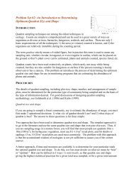
INTRODUCTION<br />
<strong>Quadrat</strong> sampling techniques are among the oldest techniques in ecology. Counts are simple<br />
to comprehend <strong>and</strong> can be used in a great variety of ways on organisms as diverse as trees,<br />
barnacles, kangaroos, seabirds, <strong>and</strong> caribou. There are only 2 basic requirements of all the<br />
techniques: 1) the area (or volume) counted is known, <strong>and</strong> 2) the organisms are relatively<br />
immobile during the counting period.<br />
The term quadrat strictly means a 4-sided figure, but in practice this term is used to mean<br />
any sampling unit, whether circular, hexagonal, or even irregular in outline, which can be<br />
placed on the ground so that % plant cover can be estimated, plants <strong>and</strong> animals counted,<br />
species listed, etc.<br />
<strong>Quadrat</strong> counts have been used extensively on plants, which rarely run away while being<br />
counted, but they are also suitable for animals if the person counting is keenly observant or<br />
has a camera. This problem set introduces the process of determining the optimum quadrat<br />
size <strong>and</strong> shape for use in monitoring programs that are estimating the abundance of plants<br />
<strong>and</strong> animals.<br />
PROCEDURES<br />
The details of quadrat sampling, including plot size, shape, number, <strong>and</strong> arrangement of<br />
sample plots, must be determined for the particular type of community being sampled <strong>and</strong><br />
on the basis of the type of information desired. For good discussions of designing quadrat<br />
sampling methodology, see Goldsmith et al. (1986) <strong>and</strong> Krebs (1999).<br />
<strong>Quadrat</strong> size <strong>and</strong> shape<br />
If you are going to sample a forest community, say to estimate the abundance of snags, you<br />
must first make 2 operational decisions: 1) what size of quadrat should I use? <strong>and</strong> 2) what<br />
shape of quadrat is best? <strong>An</strong>swers to these questions can be complex.<br />
Two approaches have been used to determine quadrat size <strong>and</strong> shape. The simplest approach<br />
is to go to the literature <strong>and</strong> use the same quadrat size <strong>and</strong> shape that everyone else uses.<br />
Thus, if you are sampling snags in a mature forest, you will find that most people use<br />
quadrats 10m x 10m (100 m 2 ); for herbaceous vegetation, most use 0.1-1.0 m 2 -sized plots;<br />
<strong>and</strong> for shrubs or saplings ≤3 m tall, 10-20 m 2 -sized plots are used most commonly. The
problem with this approach is that the accumulated wisdom of ecologists is not yet sufficient<br />
to assure you of the correct answer.<br />
A better approach, if time <strong>and</strong> resources are available, is to determine for your particular<br />
study the optimal quadrat size <strong>and</strong> shape. To do this, we first must decide on what we mean<br />
by “best” or “optimal.” Best can be defined in 3 ways: 1) statistically, as that quadrat size <strong>and</strong><br />
shape giving the highest statistical precision for a given total area sampled, or for a given total<br />
amount of time or money; 2) ecologically, as that quadrat size <strong>and</strong> shape that are most<br />
efficient to answer the question being asked; <strong>and</strong> 3) logistically, as that quadrat size <strong>and</strong> shape<br />
that are easiest to establish in the field <strong>and</strong> use. Be wary of the logistical criterion, however,<br />
since in many ecological cases the easiest approach is rarely the best. If you are investigating<br />
questions of ecological scale, the processes you are studying will dictate quadrat size, but in<br />
most cases the statistical criterion <strong>and</strong> the ecological criterion are the same. In all these cases<br />
we define<br />
highest statistical precision = lowest st<strong>and</strong>ard error of the mean<br />
= narrowest confidence interval for the mean.<br />
In almost all cases we will encounter, we should determine the quadrat size <strong>and</strong> shape that will<br />
give us the highest statistical precision. How can we do this?<br />
Let’s consider the shape question first. There are 2 conflicting problems with shape. First, the<br />
edge effect is smallest in a circular quadrat, <strong>and</strong> largest in a rectangular one. The ratio of<br />
length of edge to the area inside a quadrat changes as follows:<br />
Circle < Square < Rectangle<br />
Edge effect is important because it leads to possible counting errors. A decision must be<br />
made every time an animal or plant is at the edge of a quadrat: Is this individual inside or<br />
outside the area to be counted? This decision is often biased because most biologists prefer<br />
to count an organism rather than ignore it. Edge effects thus often produce positive biases<br />
(i.e., the numbers of organisms counted within the quadrat are higher than they should be,<br />
which could obviously lead to a population estimate that is too high). Proportionally, the<br />
more edge your plot has the more positive bias results. The general significance of possible<br />
errors of counting at the edge of a quadrat cannot be quantified because it is organism- <strong>and</strong><br />
habitat-specific. It can, however, be reduced by training. If edge effects are a significant<br />
source of error, you should choose a quadrat shape with less edge/area. But how do you<br />
know you might have an edge effect problem? Figure 1 illustrates a way of recognizing an<br />
edge effect problem. Note that there is no reason to expect any bias in mean abundance<br />
estimated from a variety of quadrat sizes <strong>and</strong> shapes. If there is no edge effect bias, we expect<br />
in an ideal world to get the same mean value regardless of the size or shape of the quadrats<br />
2
used, if the mean is expressed in the same units of area. This is important to remember:<br />
<strong>Quadrat</strong> size <strong>and</strong> shape are not about biased abundance estimates but are about narrower<br />
confidence limits. If you find a relationship like that in Figure 1 in a data set you are working<br />
on, you should immediately disqualify the smallest quadrat size from consideration to avoid<br />
bias from the edge effect.<br />
Figure 1. Edge effect bias in small quadrats. The<br />
estimated mean dry weight of grass (per 0.25<br />
m 2 ) is much higher in quadrat size 1 (0.016 m 2 )<br />
than in all other quadrat sizes. This suggests an<br />
overestimation bias due to edge effects, <strong>and</strong> that<br />
quadrat size 1 should not be used to estimate<br />
abundance of these grasses. The data are from<br />
Wiegert (1962).<br />
The second problem regarding quadrat shape is that nearly everyone has found that long,<br />
thin quadrats are better than circular or square ones of the same area. The reason for this is<br />
because of habitat heterogeneity. Long quadrats cross more patches <strong>and</strong> thus capture more<br />
of the habitat variability (something you want to do). Habitats are rarely uniform, <strong>and</strong><br />
organisms are usually distributed somewhat patchily within the overall sampling zone.<br />
Clapham (1932) counted the number of self-heal (Prunella vulgaris) plants in 1-m 2 quadrats<br />
of 2 shapes: 1m x 1m (square) <strong>and</strong> 4m x 0.25 m (rectangle). He counted 16 quadrats <strong>and</strong> got<br />
these results:<br />
<strong>Quadrat</strong> size Mean Variance SE 95% CI<br />
1m x 1m 24 565.3 5.94 ±12.65<br />
4m x 0.25m 24 333.3 4.56 ±9.71<br />
Clearly in this situation, the rectangular quadrats are more efficient than square ones (i.e., the<br />
SE is lower <strong>and</strong> the CI is narrower). Given that only 2 shapes of quadrats were tried, we do<br />
not know if even longer, thinner quadrats might be still more efficient.<br />
Not all sampling data show this preference for long, thin quadrats, <strong>and</strong> for this reason each<br />
situation should be analyzed independently. Table 1 shows data from basal area<br />
measurements on trees in a forest st<strong>and</strong> studied by Bormann (1953). The observed SD almost<br />
always falls as quadrat area increases. But if an equal total area is being sampled, the highest<br />
precision (=lowest SE) will be obtained by using 70 4m x 4m quadrats (Table 1). If, on the<br />
3
other h<strong>and</strong>, an equal number of quadrats were to be taken for each quadrat size, one would<br />
prefer the long, thin quadrat shape.<br />
Table 1. Effect of quadrat size on SD for measurements of basal area of trees in an oakhickory<br />
forest in North Carolina. The data are from Bormann (1953).<br />
<strong>Quadrat</strong> size Observed SD<br />
(m) per 4 m2 Sample sizea SE of the<br />
mean for<br />
sample size<br />
4 x 4 50.7 70 6.06<br />
4 x 10 47.3 28 8.94<br />
4 x 20 44.6 14 11.92<br />
4 x 70 41.3 4 20.65<br />
4 x 140 34.8 2 24.61<br />
aThe number of quadrats of a given size needed to sample 1,120 m2 .<br />
Two methods are available for choosing the best quadrat size statistically. Wiegert (1962)<br />
proposed a general method that can be used to determine optimal size or shape. Hendricks<br />
(1956) proposed a more restrictive method for estimating optimal size of quadrats. In both<br />
methods it is essential that data from all quadrats be st<strong>and</strong>ardized to a single unit area—for<br />
example, per m2 . This conversion is simple for means, SDs, <strong>and</strong> SEs: divide by the relative<br />
area. For example,<br />
Mean number per m2 2<br />
Mean number per 0.25m<br />
=<br />
0.25<br />
SD per m2 2<br />
SD4m<br />
=<br />
4<br />
For variances, the square of the conversion factor is used:<br />
Variance per m2 Variance per 9m<br />
= 2<br />
9<br />
2<br />
For both Wiegert’s <strong>and</strong> Hendrick’s methods, you should st<strong>and</strong>ardize all data to a common<br />
base area before testing for optimal size or shape of quadrat. They both assume further that<br />
you have tested for <strong>and</strong> eliminated quadrat sizes that give an edge effect bias. We will only<br />
deal with Wiegert’s method here.<br />
4
Wiegert’s method of determining optimum quadrat size <strong>and</strong> shape<br />
Wiegert (1962) proposed that 2 factors were of primary importance in deciding on optimal<br />
quadrat size or shape: relative variability <strong>and</strong> relative cost. In any field study, time or money<br />
would seem to be the limiting resource, <strong>and</strong> we must consider how to optimize with respect<br />
to sampling time. We will assume that time = money, <strong>and</strong> in the formulas that follow, either<br />
unit may be used. Costs of sampling have 2 components (in a simple world anyway):<br />
C = C0 + Cx,<br />
where C = Total cost for 1 sample<br />
C0 = Fixed costs or overhead<br />
Cx = Cost for taking 1 sample quadrat of size x.<br />
Fixed costs involve the time spent walking or flying between sampling points <strong>and</strong> the time<br />
spent locating a r<strong>and</strong>om point for the quadrat; these costs may be trivial in an open grassl<strong>and</strong>;<br />
they can be enormous when sampling the ocean in a large ship. The cost for taking a single<br />
quadrat may or may not vary with the size of the quadrat. Consider a simple example from<br />
Wiegert (1962) of grass biomass in quadrats of different sizes:<br />
<strong>Quadrat</strong> size (area)<br />
1 3 4 12 16<br />
Fixed cost ($) 10 10 10 10 10<br />
Cost per sample ($) 2 6 8 24 32<br />
Total cost for 1 quadrat ($) 12 16 18 34 42<br />
Relative cost for 1 quadrat 1 1.33 1.50 2.83 3.50<br />
We need to balance these costs against the relative variability of samples taken with quadrats<br />
of different sizes:<br />
Observed variance per 0.25<br />
m 2<br />
<strong>Quadrat</strong> size (area)<br />
1 3 4 12 16<br />
0.97 0.24 0.32 0.14 0.15<br />
The operational rule is, Pick the quadrat size that minimizes the product of (Relative cost) x<br />
(Relative variability).<br />
5
In this example, we begin by disqualifying quadrat size 1 because it showed a strong edge<br />
effect bias (Figure 1). Figure 2 shows that the optimal quadrat size for grass in this particular<br />
study is 3, although there is relatively little difference between the products for quadrats of<br />
size 3, 4, 12, <strong>and</strong> 16. In this case, the size 3 quadrat gives the maximum precision for the least<br />
cost.<br />
Figure 2. <strong>Determining</strong> the optimal quadrat size<br />
for sampling. The best quadrat size is that which<br />
gives the minimal value of the product of relative<br />
cost <strong>and</strong> relative variability, which is quadrat size<br />
3 in this example. <strong>Quadrat</strong> size 1 is plotted here<br />
for illustration, even though this quadrat size is<br />
disqualified because of edge effects. Data here are<br />
dry weights of grasses in quadrats of variable size.<br />
Data are from Wiegert (1962).<br />
Let’s work through an example from start to finish. The data we are using comes from<br />
Pringle’s (1984) study of seaweed (Chondrus crispus) biomass. As you can see from Table 2,<br />
Pringle tried quadrats of several different sizes in a pilot study to assist him in selecting the<br />
most appropriate-sized quadrat.<br />
Table 2. Data to determine optimal quadrat size for biomass estimates of the seaweed,<br />
Chondrus crispus (from Pringle 1984).<br />
<strong>Quadrat</strong> size<br />
(m)<br />
Sample size a<br />
Mean<br />
biomass b<br />
(g)<br />
SD b<br />
SE of the<br />
mean b<br />
Time to<br />
take 1<br />
sample<br />
(min)<br />
0.5 x 0.5 79 1524 1022 115 6.7<br />
1 x 1 20 1314 963 215 12.0<br />
1.25 x 1.25 13 1037 605 168 13.2<br />
1.5 x 1.5 9 1116 588 196 11.4<br />
1.73 x 1.73 6 2021 800 327 33.0<br />
2 x 2 5 1099 820 367 23.0<br />
a Sample sizes are approximately the number to make a total sampling area of 20 m 2 .<br />
b All expressed per m 2 .<br />
If we neglect any fixed costs <strong>and</strong> use the time to take 1 sample as the total cost, we can<br />
calculate the relative cost for each quadrat size as<br />
6
Relative cost =<br />
Time to take 1 sample of a givensize<br />
Minimum time to take 1 sample<br />
Equation 1<br />
In this case the minimum time = 6.7 minutes for the 0.5 x 0.5 quadrat (that shouldn’t be<br />
surprising). We can also express the variance [=(SD) 2 ] on a relative scale:<br />
2<br />
(SD)<br />
Relative variance = 2<br />
Equation 2<br />
(Minimum SD)<br />
In this case, the minimum variance occurs for quadrats of 1.5 x 1.5 m. We obtain for these<br />
data:<br />
<strong>Quadrat</strong> size<br />
(m)<br />
Relative<br />
variance<br />
Relative<br />
cost<br />
Product of<br />
relative variance<br />
<strong>and</strong> relative cost<br />
0.5 x 0.5 3.02 1.00 3.02<br />
1 x 1 2.68 1.79 4.80<br />
1.25 x 1.25 1.06 1.97 2.09<br />
1.5 x 1.5 1.00 1.70 1.70<br />
1.73 x 1.73 1.85 4.93 9.12<br />
2 x 2 1.94 3.43 6.65<br />
The operational rule is to pick the quadrat size with minimal product of cost x variance, <strong>and</strong><br />
this is clearly the 1.5 x 1.5 m quadrat, which is the optimal quadrat size for this particular<br />
sampling area.<br />
There is a slight suggestion of a positive bias in the mean biomass estimates for the smallest<br />
quadrats (Table 2), but this was not tested for by Pringle. Optimal quadrat shape could be<br />
decided in exactly the same way as quadrat size.<br />
Would there ever be a time when you might not want to determine optimum quadrat size<br />
<strong>and</strong> shape? Sampling plant <strong>and</strong> animal populations with quadrats is done for many different<br />
reasons, <strong>and</strong> it is important to ask when you might be advised to ignore the<br />
recommendations for quadrat size <strong>and</strong> shape that arise from Wiegert’s method.<br />
There are 2 common situations when you may wish to ignore these recommendations. In<br />
some cases you will wish to compare your data with older data gathered with a specific<br />
quadrat size <strong>and</strong> shape. Even if the older quadrat size <strong>and</strong> shape are inefficient, you may be<br />
advised, for comparative purposes, to continue using the old quadrat size <strong>and</strong> shape. In<br />
principle this is not required, as long as no bias is introduced by a change in quadrat size. But<br />
in practice, many biologists are more comfortable using the same quadrats as the earlier<br />
7
studies. This can become a more serious problem in a long-term monitoring program in<br />
which a poor choice of quadrat size in the early stages could condemn the whole project to<br />
wasting time <strong>and</strong> resources with inefficient sampling procedures.<br />
If you are sampling several habitats, sampling for many different species, <strong>and</strong>/or sampling<br />
over several seasons, you may find that these procedures result in a recommendation for a<br />
different size <strong>and</strong> shape of quadrat for each situation. It may be impossible to do this for<br />
logistical reasons, <strong>and</strong> thus you may have to compromise.<br />
NOW YOU DO IT<br />
Exercise #1: A field plot was located in the subalpine zone of Rocky<br />
Mountain National Park, Colorado <strong>and</strong> divided into 16 quadrats of 1-m 2 .<br />
The numbers of American bistort, Polygonum bistortoides, were<br />
counted in each quadrat with these results:<br />
3 0 5 1<br />
5 7 2 0<br />
3 2 0 7<br />
3 3 3 4<br />
Calculate the precision (i.e., SE of the mean <strong>and</strong> CI) of sampling this universe with 2 possible<br />
shapes of 4-m 2 quadrats: 2m x 2m <strong>and</strong> 4m x 1m.<br />
Exercise #2: Using the mapped population of a 17,860-m 2 (1.8 ha) st<strong>and</strong> of hardwoods in<br />
northern Minnesota provided, use Wiegert’s method to determine the optimum quadrat size<br />
to determine the number of balsam fir trees (species #1 on the map). Table 3 contains the<br />
quadrat sizes you will compare, the required sample sizes for each quadrat size (yes, you will<br />
need to sample at the intensity indicated), <strong>and</strong> the estimated time required to take 1 sample<br />
at each quadrat size (these numbers are provided <strong>and</strong> are mere guesses of the amount of time<br />
it would actually take to search a quadrat of each size for balsam fir trees). Notice that<br />
sample size is being held constant relative to the quadrat size so that each quadrat size is<br />
sampling the same area. We will discuss ways of determining sample sizes latter. You need to<br />
calculate the mean number of balsam fir trees, the SD, <strong>and</strong> the SE of the mean for each<br />
quadrat size. Record your data in Table 3. With these data, use Equations 1 <strong>and</strong> 2 to<br />
determine optimum quadrat size. Record your calculations in Table 4.<br />
8
Use the 3 quadrats on the overhead transparency provided. <strong>Quadrat</strong>s could be located<br />
r<strong>and</strong>omly using the 2 numbered axes placed along the edges of the sampling frame. As you<br />
can see, the axes divide the sampling frame into cells. Using a r<strong>and</strong>om numbers table, you<br />
could select a pair of numbers (x <strong>and</strong> y) <strong>and</strong> use these numbers to place your quadrat on the<br />
map. Perhaps you would place the lower left corner of each quadrat on each r<strong>and</strong>omlylocated<br />
point. Don’t forget to answer the 3 questions below.<br />
Table 3. Optimal quadrat size for population estimates of balsam fir.<br />
<strong>Quadrat</strong> size<br />
(m)<br />
Sample size a<br />
Mean<br />
number of<br />
balsam fir b<br />
SD b<br />
SE of the<br />
mean b<br />
Time to<br />
search 1<br />
quadrat<br />
(min)<br />
10m x 10m 50 5<br />
25m x 25m 8 30<br />
50m x 50m 2 125<br />
a Sample sizes are the number of quadrats to make a total sampling area of 5,000m 2 .<br />
b All expressed per m 2 .<br />
Table 4. Wiegert’s method to determine optimal quadrat size for counting balsam fir in a<br />
northern hardwood st<strong>and</strong>.<br />
<strong>Quadrat</strong> size<br />
(m)<br />
10m x 10m<br />
25m x 25m<br />
50m x 50m<br />
QUESTIONS:<br />
Relative<br />
variance<br />
Relative<br />
cost<br />
Product of<br />
relative variance<br />
<strong>and</strong> relative cost<br />
1. What are the SE <strong>and</strong> CI for the 2 quadrate sizes used in exercise #1?<br />
9
2. What is the most optimum quadrat size to count balsam fir in this northern hardwood<br />
st<strong>and</strong>?<br />
3. How would you go about determining optimum quadrat shape? Work up an approach<br />
<strong>and</strong> do it. A couple of blank overhead transparencies are provided for your use. What is<br />
the most optimum quadrat shape to count balsam fir in this northern hardwood st<strong>and</strong>?<br />
ACKNOWLEDGEMENTS<br />
The bulk of this problem set was taken from Krebs (1999), particularly chapter 4.<br />
LITERATURE CITED<br />
Bormann, F.H. 1953. The statistical efficiency of sample plot size <strong>and</strong> shape in forest ecology.<br />
Ecology 34:474-487.<br />
Clapham, A. R. 1932. The form of the observational unit in quantitative ecology. Journal of<br />
Ecology 20:192-197.<br />
Goldsmith, F.B., C.M. Harrison, <strong>and</strong> A.J. Morton. 1986. Description <strong>and</strong> analysis of<br />
vegetation. Pages 437-524 in P.D. Moore <strong>and</strong> S.B. Chapman, editors. Methods in plant<br />
ecology. Blackwell Scientific Publications, Oxford, Engl<strong>and</strong>.<br />
Krebs, C.J. 1999. Ecological methodology. Addison-Wesley Educational Publishers, Inc.,<br />
Menlo Park, CA. 620 pp.<br />
Pringle, J.D. 1984. Efficiency estimates for various quadrat sizes used in benthic sampling.<br />
Canadian Journal of Fisheries <strong>and</strong> Aquatic Sciences 41:1485-1489.<br />
Wiegert, R.G. 1962. The selection of an optimum quadrat size for sampling the st<strong>and</strong>ing crop<br />
of grasses <strong>and</strong> forbs. Ecology 43:125-129.<br />
10