- Page 3 and 4:
ADVANCES IN PSYCHOLOGY 104 Editors:
- Page 5 and 6:
NORTH-HOLLAND ELSEVIER SCIENCE B.V.
- Page 7 and 8:
vi THE GRASPING HAND including comp
- Page 9 and 10:
viii THE GRASPING HAND Finally, all
- Page 11 and 12:
X THE GRASPING HAND 4.2 Task Plans
- Page 13 and 14:
xii THE GRASPING HAND Part I11 CONS
- Page 15 and 16:
xiv Figure 1.1 Figure 1.2 Figure 1.
- Page 17 and 18:
XVi THE GRASPING HAND Figure 6.12 F
- Page 19 and 20:
This Page Intentionally Left Blank
- Page 21 and 22:
This Page Intentionally Left Blank
- Page 23 and 24:
4 WHAT IS PREHENSION? The hand itse
- Page 25 and 26:
6 WHAT IS PREHENSION? continue in t
- Page 27 and 28:
8 WHAT IS PREHENSION? movement. Dom
- Page 29 and 30:
10 WHAT IS PREHENSION? Today, with
- Page 31 and 32:
12 WHAT IS PREHENSION? prehensile b
- Page 33 and 34:
This Page Intentionally Left Blank
- Page 35 and 36:
16 WHAT IS PREHENSION? (1988) refer
- Page 37 and 38:
18 WHAT IS PREHENSION? in Table 2.1
- Page 39 and 40:
20 WHAT IS PREHENSION? Table 2.1 Pr
- Page 41 and 42:
22 WHAT IS PREHENSION? Schlesinger
- Page 43 and 44:
24 WHAT IS PREHENSION? A. POWER GRA
- Page 45 and 46:
emphasis on Grasp emphasis on secur
- Page 47 and 48:
28 WHAT IS PREHENSION? (screwing on
- Page 49 and 50:
30 WHAT IS PREHENSION? suggested th
- Page 51 and 52:
Figure 2.5 Prehensile postures cons
- Page 53 and 54:
Figure 2.7 Oppositions can be descr
- Page 55 and 56:
36 WHAT IS PREHENSION? Many posture
- Page 57 and 58:
38 WHAT IS PREHENSION? and unwieldy
- Page 59 and 60:
40 WHAT IS PREHENSION? d Figure 2.9
- Page 61 and 62:
42 WHAT IS PREHENSION? quired oppos
- Page 63 and 64:
44 WHAT IS PREHENSION? sion; i.e.,
- Page 65 and 66:
46 WHAT IS PREHENSION? impossible t
- Page 67 and 68:
This Page Intentionally Left Blank
- Page 69 and 70:
50 THE PHASES OF PREHENSION V cm/s
- Page 71 and 72:
52 THE PHASES OF PREHENSION - 0 200
- Page 73 and 74:
54 THE PHASES OF PREHENSION recogni
- Page 75 and 76:
56 THE PHASES OF PREHENSION Executi
- Page 77 and 78:
58 THE PHASES OF PREHENSION untary
- Page 79 and 80:
60 THE PHASES OF PREHENSION isting
- Page 81 and 82:
This Page Intentionally Left Blank
- Page 83 and 84:
64 THE PHASES OF PREHENSION ence, w
- Page 85 and 86:
66 THE PHASES OF PREHENSION being p
- Page 87 and 88:
68 (sticks up) THE PHASES OF PREHEN
- Page 89 and 90:
70 THE PHASES OF PREHENSION (right
- Page 91 and 92:
72 THE PHASES OF PREHENSION organiz
- Page 93 and 94:
74 THE PHASES OF PREHENSION movemen
- Page 95 and 96:
76 THE PHASES OF PREHENSION and bas
- Page 97 and 98:
78 THE PHASES OF PREHENSION Figure
- Page 99 and 100:
80 THE PHASES OF PREHENSION Again,
- Page 101 and 102:
82 THE PHASES OF PREHENSION c Oppos
- Page 103 and 104:
84 THE PHASES OF PREHENSION the mac
- Page 105 and 106:
86 THE PHASES OF PREHENSION (surfac
- Page 107 and 108:
88 THE PHASES OF PREHENSION influen
- Page 109 and 110:
90 THE PHASES OF PREHENSION able to
- Page 111 and 112:
92 THE PHASES OF PREHENSION A Pfing
- Page 113 and 114:
94 THE PHASES OF PREHENSION forces,
- Page 115 and 116:
- Computed activation of arm muscle
- Page 117 and 118:
98 THE PHASES OF PREHENSION were in
- Page 119 and 120:
100 THE PHASES OF PREHENSION Figure
- Page 121 and 122:
102 THE PHASES OF PREHENSION same t
- Page 123 and 124:
104 THE PHASES OF PREHENSION OBJECT
- Page 125 and 126:
106 THE PHASES OF PREHENSION planni
- Page 127 and 128:
This Page Intentionally Left Blank
- Page 129 and 130:
110 THE PHASES OF PREHENSION antici
- Page 131 and 132:
112 THE PHASES OF PREHENSION and te
- Page 133 and 134:
114 THE PHASES OF PREHENSION presen
- Page 135 and 136:
116 THE PHASES OF PREHENSION determ
- Page 137 and 138:
118 THE PHASES OF PREHENSION 5.3 Co
- Page 139 and 140:
120 THE PHASES OF PREHENSION tance
- Page 141 and 142:
122 THE PHASES OF PREHENSION where
- Page 143 and 144:
124 THE PHASES OF PREHENSION Figure
- Page 145 and 146:
126 THE PHASES OF PREHENSION A B 18
- Page 147 and 148:
128 THE PHASES OF PREHENSION where
- Page 149 and 150:
130 THE PHASES OF PREHENSION SR = .
- Page 151 and 152:
132 THE PHASES OF PREHENSION MODEL
- Page 153 and 154:
134 THE PHASES OF PREHENSION A B Fi
- Page 155 and 156:
136 THE PHASES OF PREHENSION to mus
- Page 157 and 158:
138 THE PHASES OF PREHENSION method
- Page 159 and 160:
140 THE PHASES OF PREHENSION tire b
- Page 161 and 162:
142 THE PHASES OF PREHENSION torque
- Page 163 and 164:
144 THE PHASES OF PREHENSION relate
- Page 165 and 166:
146 THE PHASES OF PREHENSION the ob
- Page 167 and 168:
148 THE PHASES OF PREHENSION abilit
- Page 169 and 170:
150 THE PHASES OF PREHENSION +60 1
- Page 171 and 172:
152 THE PHASES OF PREHENSION result
- Page 173 and 174:
154 THE PHASES OF PREHENSION the di
- Page 175 and 176:
156 THE PHASES OF PREHENSION crease
- Page 177 and 178:
158 THE PHASES OF PREHENSION betwee
- Page 179 and 180:
160 50 1 THE PHASES OF PREHENSION 1
- Page 181 and 182:
162 THE PHASES OF PREHENSION positi
- Page 183 and 184:
- Velocity - Acceleration s-L 1400
- Page 185 and 186:
166 THE PHASES OF PREHENSION vocal
- Page 187 and 188:
168 THE PHASES OF PREHENSION C z3Oo
- Page 189 and 190:
170 THE PHASES OF PREHENSION 150 T
- Page 191 and 192:
172 THE PHASES OF PREHENSION T 150
- Page 193 and 194:
174 THE PHASES OF PREHENSION grasp
- Page 195 and 196:
176 AREA 7 (IPS) THE PHASES OF PREH
- Page 197 and 198:
178 THE PHASES OF PREHENSION books
- Page 199 and 200:
180 THE PHASES OF PREHENSION h .r?.
- Page 201 and 202:
182 THE PHASES OF PREHENSION A B C
- Page 203 and 204:
184 THE PHASES OF PREHENSION (1982b
- Page 205 and 206:
186 THE PHASES OF PREHENSION _ - B
- Page 207 and 208:
188 THE PHASES OF PREHENSION A +6 1
- Page 209 and 210:
190 THE PHASES OF PREHENSION activa
- Page 211 and 212:
192 THE PHASES OF PREHENSION shape,
- Page 213 and 214:
194 THE PHASES OF PREHENSION the st
- Page 215 and 216:
196 THE PHASES OF PREHENSION collap
- Page 217 and 218:
198 THE PHASES OF PREHENSION Obi& T
- Page 219 and 220:
200 THE PHASES OF PREHENSION might
- Page 221 and 222:
This Page Intentionally Left Blank
- Page 223 and 224:
204 THE PHASES OF PREHENSION about
- Page 225 and 226:
206 THE PHASES OF PREHENSION hands
- Page 227 and 228:
208 THE PHASES OF PREHENSION Epider
- Page 229 and 230:
210 THE PHASES OF PREHENSION the pe
- Page 231 and 232:
212 THE PHASES OF PREHENSION FtiYsT
- Page 233 and 234:
214 THE PHASES OF PREHENSION focusi
- Page 235 and 236:
216 THE PHASES OF PREHENSION thermo
- Page 237 and 238:
218 THE PHASES OF PREHENSION nonner
- Page 239 and 240:
220 THE PHASES OF PREHENSION hot-wa
- Page 241 and 242:
222 THE PHASES OF PREHENSION which,
- Page 243 and 244:
224 THE PHASES OF PREHENSION which
- Page 245 and 246:
226 THE PHASES OF PREHENSION for FA
- Page 247 and 248:
228 THE PHASES OF PREHENSION differ
- Page 249 and 250:
230 THE PHASES OF PREHENSION (see C
- Page 251 and 252:
232 THE PHASES OF PREHENSION LATERA
- Page 253 and 254:
234 THE PHASES OF PREHENSION more a
- Page 255 and 256:
236 THE PHASES OF PREHENSION A Poin
- Page 257 and 258:
238 THE PHASES OF PREHENSION Figure
- Page 259 and 260:
240 THE PHASES OF PREHENSION 6.3.2
- Page 261 and 262:
242 THE PHASES OF PREHENSION equati
- Page 263 and 264:
244 THE PHASES OF PREHENSION necess
- Page 265 and 266:
246 THE PHASES OF PREHENSION graspi
- Page 267 and 268:
248 A THE PHASES OF PREHENSION Figu
- Page 269 and 270:
250 z J 2 0 c .- Q el X A THE PHASE
- Page 271 and 272:
252 THE PHASES OF PREHENSION respec
- Page 273 and 274:
254 THE PHASES OF PREHENSION Z 151
- Page 275 and 276:
256 THE PHASES OF PREHENSION mechan
- Page 277 and 278:
258 THE PHASES OF PREHENSION see He
- Page 279 and 280:
260 THE PHASES OF PREHENSION might
- Page 281 and 282:
262 THE PHASES OF PREHENSION long a
- Page 283 and 284:
264 THE PHASES OF PREHENSION with u
- Page 285 and 286:
266 THE PHASES OF PREHENSION Table
- Page 287 and 288:
268 THE PHASES OF PREHENSION system
- Page 289 and 290:
270 THE PHASES OF PREHENSION In cla
- Page 291 and 292:
Table 6.6 Elliott & Connolly (1984)
- Page 293 and 294:
274 THE PHASES OF PREHENSION shape
- Page 295 and 296:
276 THE PHASES OF PREHENSION In imp
- Page 297 and 298:
278 THE PHASES OF PREHENSION cause
- Page 299 and 300:
aie3 INTRINSIC - mughnesn aspect of
- Page 301 and 302:
This Page Intentionally Left Blank
- Page 303 and 304:
284 THE PHASES OF PREHENSION percei
- Page 305 and 306:
286 THE PHASES OF PREHENSION Figure
- Page 307 and 308:
288 THE PHASES OF PREHENSION approa
- Page 309 and 310:
290 5. 6. 7. 8. 9. 10. 11. 12. 13.
- Page 311 and 312:
292 THE PHASES OF PREHENSION Fitts
- Page 313 and 314:
294 THE PHASES OF PREHENSION accele
- Page 315 and 316:
296 THE PHASES OF PREHENSION 27. Ce
- Page 317 and 318:
298 THE PHASES OF PREHENSION charac
- Page 319 and 320:
300 THE PHASES OF PREHENSION are se
- Page 321 and 322:
This Page Intentionally Left Blank
- Page 323 and 324:
This Page Intentionally Left Blank
- Page 325 and 326:
306 CONSTRAINTS AND PHASES Table 8.
- Page 327 and 328:
308 CONSTRAINTS AND PHASES the inde
- Page 329 and 330:
310 CONSTRAINTS AND PHASES While th
- Page 331 and 332:
312 CONSTRAINTS AND PHASES for a gi
- Page 333 and 334:
314 CONSTRAINTS AND PHASES fine, su
- Page 335 and 336:
316 CONSTRAINTS AND PHASES level fi
- Page 337 and 338:
318 CONSTRAINTS AND PHASES spent in
- Page 339 and 340:
z I l l I 0 Y "K ' ,------ Sensorim
- Page 341 and 342:
322 CONSTRAINTS AND PHASES componen
- Page 343 and 344:
324 CONSTRAINTS AND PHASES and the
- Page 345 and 346:
326 CONSTRAINTS AND PHASES 8.6 Summ
- Page 347 and 348:
This Page Intentionally Left Blank
- Page 349 and 350:
330 CONSTRAINTS AND PHASES 9.1 The
- Page 351 and 352:
332 CONSTRAINTS AND PHASES b) impar
- Page 353 and 354: 334 CONSTRAINTS AND PHASES The defi
- Page 355 and 356: 336 CONSTRAINTS AND PHASES less pre
- Page 357 and 358: 338 CONSTRAINTS AND PHASES transpor
- Page 359 and 360: Opposition Space level Sensorimotor
- Page 361 and 362: 342 CONSTRAINTS AND PHASES 9.3 Futu
- Page 363 and 364: 344 CONSTRAINTS AND PHASES scientif
- Page 365 and 366: This Page Intentionally Left Blank
- Page 367 and 368: This Page Intentionally Left Blank
- Page 369 and 370: 350 Appendices Anterior (ventral):
- Page 371 and 372: 352 Appendices =!- / Scapula Acromi
- Page 373 and 374: 354 A pp e n dices Table A.l Degree
- Page 375 and 376: 356 Appendices Table A.l Degrees of
- Page 377 and 378: 358 Appendices Flexion: to bend or
- Page 379 and 380: 360 A pp e n dic e s Table A.2 Join
- Page 381 and 382: 362 A pp e It dices Elbow flex ext
- Page 383 and 384: 364 A pp e n dices Table A.2 Joints
- Page 385 and 386: 366 A pp e n dic e s Table A.3 Inne
- Page 387 and 388: This Page Intentionally Left Blank
- Page 389 and 390: 370 Appendices Table B.l Prehensile
- Page 391 and 392: 372 Appendices ...... ........... t
- Page 393 and 394: 374 Appendices features of the huma
- Page 395 and 396: 376 Appendices fingers (Kamakura et
- Page 397 and 398: 378 Appendices Table B.3 Postures c
- Page 399 and 400: 380 Appendices opposition, is Napie
- Page 401 and 402: 382 A pp e n dic e s relationships
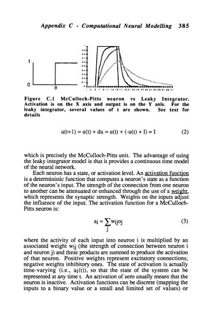
- Page 403: 384 A pp e n dic e s C.2 Artificial
- Page 407 and 408: 388 A pp e n dices processing. This
- Page 409 and 410: 390 Appendices between two units in
- Page 411 and 412: 392 A pp e n dic e s where q is a s
- Page 413 and 414: 394 A pp e It d ic e s training set
- Page 415 and 416: 396 A pp e It dic e s units. Also,
- Page 417 and 418: 398 Appendices only sense is vision
- Page 419 and 420: 400 A pp e n dices of computations
- Page 421 and 422: 402 A pp e n dic e s satisfy active
- Page 423 and 424: 404 Appendices biceps, and shoulder
- Page 425 and 426: 406 Appendices Table D.l Commercial
- Page 427 and 428: 408 Appendices Table D.2 Commercial
- Page 429 and 430: 410 Appendices Sears et al., 1989).
- Page 431 and 432: 412 A ppe It dic e s are active, wh
- Page 433 and 434: 414 A ppen die es automatic lock wh
- Page 435 and 436: 416 A pp e n dices between the thum
- Page 437 and 438: 418 Appendices D.3.1 Stanford/JPL h
- Page 439 and 440: 420 A pp e n dices D.3.3 Belgrade/U
- Page 441 and 442: This Page Intentionally Left Blank
- Page 443 and 444: 424 THE GRASPING HAND Arbib, M.A. (
- Page 445 and 446: 426 THE GRASPING HAND Bullock, D.,
- Page 447 and 448: 428 THE GRASPING HAND Cutkosky, M.R
- Page 449 and 450: 430 THE GRASPING HAND Focillon, H.
- Page 451 and 452: 432 THE GRASPING HAND Gordon, A.M.,
- Page 453 and 454: 434 THE GRASPING HAND Hollerbach, J
- Page 455 and 456:
436 THE GRASPING HAND Jeannerod, M.
- Page 457 and 458:
438 THE GRASPING HAND Kamakura, N.,
- Page 459 and 460:
440 THE GRASPING HAND Landsmeer, J.
- Page 461 and 462:
442 THE GRASPING HAND MacKenzie, C.
- Page 463 and 464:
444 THE GRASPING HAND Moore, D.F. (
- Page 465 and 466:
446 THE GRASPING HAND Phillips, C.G
- Page 467 and 468:
448 THE GRASPING HAND Rumelhart, D.
- Page 469 and 470:
450 THE GRASPING HAND disconnection
- Page 471 and 472:
452 THE GRASPING HAND Weir, P.L. (1
- Page 473 and 474:
This Page Intentionally Left Blank
- Page 475 and 476:
456 THE GRASPING HAND Childress, D.
- Page 477 and 478:
458 THE GRASPING HAND Johansson, R.
- Page 479 and 480:
460 THE GRASPING HAND Proteau, L.,
- Page 481 and 482:
This Page Intentionally Left Blank
- Page 483 and 484:
464 THE GRASPING HAND level, of map
- Page 485 and 486:
466 THE GRASPING HAND a h Generaliz
- Page 487 and 488:
468 THE GRASPING HAND Forces. Force
- Page 489 and 490:
470 THE GRASPING HAND han& Robotics
- Page 491 and 492:
472 THE GRASPING HAND and force coo
- Page 493 and 494:
474 THE GRASPING HAND and task requ
- Page 495 and 496:
476 THE GRASPING HAND Pen, as grasp
- Page 497 and 498:
478 THE GRASPING HAND Screwdriver,
- Page 499 and 500:
480 THE GRASPING HAND and oppositio
- Page 501:
482 THE GRASPING HAND and grasping,


