Research Methodology - Dr. Krishan K. Pandey
Research Methodology - Dr. Krishan K. Pandey Research Methodology - Dr. Krishan K. Pandey
Testing of Hypotheses-II 309 (ii) If N is larger than 7, we may use χ 2 value to be worked out as: χ 2 = k(N – 1). W with d.f. = (N – 1) for judging W’s significance at a given level in the usual way of using χ 2 values. (f) Significant value of W may be interpreted and understood as if the judges are applying essentially the same standard in ranking the N objects under consideration, but this should never mean that the orderings observed are correct for the simple reason that all judges can agree in ordering objects because they all might employ ‘wrong’ criterion. Kendall, therefore, suggests that the best estimate of the ‘true’ rankings of N objects is provided, when W is significant, by the order of the various sums of ranks, R j . If one accepts the criterion which the various judges have agreed upon, then the best estimate of the ‘true’ ranking is provided by the order of the sums of ranks. The best estimate is related to the lowest value observed amongst R j . This can be illustrated with the help of an example. Illustration 9 Seven individuals have been assigned ranks by four judges at a certain music competition as shown in the following matrix: Individuals A B C D E F G Judge 1 1 3 2 5 7 4 6 Judge 2 2 4 1 3 7 5 6 Judge 3 3 4 1 2 7 6 5 Judge 4 1 2 5 4 6 3 7 Is there significant agreement in ranking assigned by different judges? Test at 5% level. Also point out the best estimate of the true rankings. Solution: As there are four sets of rankings, we can work out the coefficient of concordance (W) for judging significant agreement in ranking by different judges. For this purpose we first develop the given matrix as under: Table 12.9 K = 4 Individuals ∴ N = 7 A B C D E F G Judge 1 1 3 2 5 7 4 6 Judge 2 2 4 1 3 7 5 6 Judge 3 3 4 1 2 7 6 5 Judge 4 1 2 5 4 6 3 7 Sum of ranks (R ) 7 13 9 14 27 18 24 ∑ R = j j dRj − Rji 2 81 9 49 4 121 4 64 ∴ s = 332 112
310 Research Methodology Q R j R = N ∑ Q s = 332 j 112 = = 7 16 s 332 332 ∴ W = = = = = 1 1 16 k N − N 4 7 − 7 12 12 12 336 332 0. 741 2 3 2 3 448 e j bge j b g To judge the significance of this W, we look into the Table No. 9 given in appendix for finding the value of s at 5% level for k = 4 and N = 7. This value is 217.0 and thus for accepting the null hypothesis (H 0 ) that k sets of rankings are independent) our calculated value of s should be less than 217. But the worked out value of s is 332 which is higher than the table value which fact shows that W = 0.741 is significant. Hence, we reject the null hypothesis and infer that the judges are applying essentially the same standard in ranking the N objects i.e., there is significant agreement in ranking by different judges at 5% level in the given case. The lowest value observed amongst R j is 7 and as such the best estimate of true rankings is in the case of individual A i.e., all judges on the whole place the individual A as first in the said music competition. Illustration 10 Given is the following information: k = 13 N = 20 W = 0.577 Determine the significance of W at 5% level. Solution: As N is larger than 7, we shall workout the value of χ 2 for determining W’s significance as under: ∴ or χ 2 = k(N – 1)W with N – 1 degrees of freedom χ 2 = 13(20 – 1) (0.577) χ 2 = (247) (0.577) = 142.52 Table value of χ 2 at 5% level for N – 1 = 20 – 1 = 19 d.f. is 30.144 but the calculated value of χ 2 is 142.52 and this is considerably higher than the table value. This does not support the null hypothesis of independence and as such we can infer that W is significant at 5% level. RELATIONSHIP BETWEEN SPEARMAN’S r ’s AND KENDALL’S W As stated above, W is an appropriate measure of studying the degree of association among three or more sets of ranks, but we can as well determine the degree of association among k sets of rankings by averaging the Spearman’s correlation coefficients (r’s) between all possible pairs (i.e., k C 2 or k (k – 1)/2) of rankings keeping in view that W bears a linear relation to the average r’s taken over
- Page 276 and 277: Analysis of Variance and Co-varianc
- Page 278 and 279: Analysis of Variance and Co-varianc
- Page 280 and 281: Analysis of Variance and Co-varianc
- Page 282 and 283: Analysis of Variance and Co-varianc
- Page 284 and 285: Analysis of Variance and Co-varianc
- Page 286 and 287: Analysis of Variance and Co-varianc
- Page 288 and 289: Analysis of Variance and Co-varianc
- Page 290 and 291: Analysis of Variance and Co-varianc
- Page 292 and 293: Analysis of Variance and Co-varianc
- Page 294 and 295: Analysis of Variance and Co-varianc
- Page 296 and 297: Analysis of Variance and Co-varianc
- Page 298 and 299: Analysis of Variance and Co-varianc
- Page 300 and 301: Testing of Hypotheses-II 283 12 Tes
- Page 302 and 303: Testing of Hypotheses-II 285 Illust
- Page 304 and 305: Testing of Hypotheses-II 287 Table
- Page 306 and 307: Testing of Hypotheses-II 289 fact,
- Page 308 and 309: Testing of Hypotheses-II 291 The te
- Page 310 and 311: Testing of Hypotheses-II 293 Pair B
- Page 312 and 313: Testing of Hypotheses-II 295 Table
- Page 314 and 315: Testing of Hypotheses-II 297 Illust
- Page 316 and 317: Testing of Hypotheses-II 299 Soluti
- Page 318 and 319: Testing of Hypotheses-II 301 r = nu
- Page 320 and 321: Testing of Hypotheses-II 303 where
- Page 322 and 323: Testing of Hypotheses-II 305 Table
- Page 324 and 325: Testing of Hypotheses-II 307 We now
- Page 328 and 329: Testing of Hypotheses-II 311 all po
- Page 330 and 331: Testing of Hypotheses-II 313 CONCLU
- Page 332 and 333: Multivariate Analysis Techniques 31
- Page 334 and 335: Multivariate Analysis Techniques 31
- Page 336 and 337: Multivariate Analysis Techniques 31
- Page 338 and 339: Multivariate Analysis Techniques 32
- Page 340 and 341: Multivariate Analysis Techniques 32
- Page 342 and 343: Multivariate Analysis Techniques 32
- Page 344 and 345: Multivariate Analysis Techniques 32
- Page 346 and 347: Multivariate Analysis Techniques 32
- Page 348 and 349: Multivariate Analysis Techniques 33
- Page 350 and 351: Multivariate Analysis Techniques 33
- Page 352 and 353: Multivariate Analysis Techniques 33
- Page 354 and 355: Multivariate Analysis Techniques 33
- Page 356 and 357: Multivariate Analysis Techniques 33
- Page 358 and 359: Multivariate Analysis Techniques 34
- Page 360 and 361: Appendix Summary Chart: Showing the
- Page 362 and 363: Interpretation and Report Writing 3
- Page 364 and 365: Interpretation and Report Writing 3
- Page 366 and 367: Interpretation and Report Writing 3
- Page 368 and 369: Interpretation and Report Writing 3
- Page 370 and 371: Interpretation and Report Writing 3
- Page 372 and 373: Interpretation and Report Writing 3
- Page 374 and 375: Interpretation and Report Writing 3
310 <strong>Research</strong> <strong>Methodology</strong><br />
Q R<br />
j<br />
R<br />
=<br />
N<br />
∑<br />
Q s = 332<br />
j<br />
112<br />
= =<br />
7<br />
16<br />
s<br />
332 332<br />
∴ W =<br />
=<br />
= = =<br />
1<br />
1<br />
16<br />
k N − N 4 7 − 7<br />
12<br />
12 12 336<br />
332<br />
0. 741<br />
2 3 2 3<br />
448<br />
e j bge j b g<br />
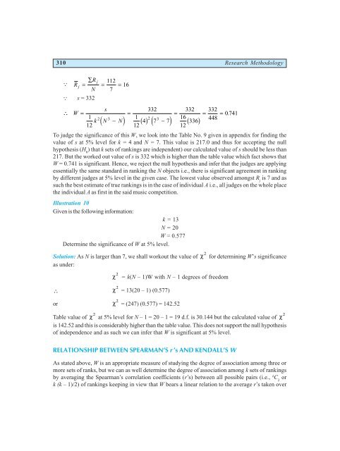
To judge the significance of this W, we look into the Table No. 9 given in appendix for finding the<br />
value of s at 5% level for k = 4 and N = 7. This value is 217.0 and thus for accepting the null<br />
hypothesis (H 0 ) that k sets of rankings are independent) our calculated value of s should be less than<br />
217. But the worked out value of s is 332 which is higher than the table value which fact shows that<br />
W = 0.741 is significant. Hence, we reject the null hypothesis and infer that the judges are applying<br />
essentially the same standard in ranking the N objects i.e., there is significant agreement in ranking<br />
by different judges at 5% level in the given case. The lowest value observed amongst R j is 7 and as<br />
such the best estimate of true rankings is in the case of individual A i.e., all judges on the whole place<br />
the individual A as first in the said music competition.<br />
Illustration 10<br />
Given is the following information:<br />
k = 13<br />
N = 20<br />
W = 0.577<br />
Determine the significance of W at 5% level.<br />
Solution: As N is larger than 7, we shall workout the value of χ 2 for determining W’s significance<br />
as under:<br />
∴<br />
or<br />
χ 2 = k(N – 1)W with N – 1 degrees of freedom<br />
χ 2 = 13(20 – 1) (0.577)<br />
χ 2 = (247) (0.577) = 142.52<br />
Table value of χ 2 at 5% level for N – 1 = 20 – 1 = 19 d.f. is 30.144 but the calculated value of χ 2<br />
is 142.52 and this is considerably higher than the table value. This does not support the null hypothesis<br />
of independence and as such we can infer that W is significant at 5% level.<br />
RELATIONSHIP BETWEEN SPEARMAN’S r ’s AND KENDALL’S W<br />
As stated above, W is an appropriate measure of studying the degree of association among three or<br />
more sets of ranks, but we can as well determine the degree of association among k sets of rankings<br />
by averaging the Spearman’s correlation coefficients (r’s) between all possible pairs (i.e., k C 2 or<br />
k (k – 1)/2) of rankings keeping in view that W bears a linear relation to the average r’s taken over


