Research Methodology - Dr. Krishan K. Pandey
Research Methodology - Dr. Krishan K. Pandey Research Methodology - Dr. Krishan K. Pandey
Testing of Hypotheses-II 293 Pair Brand A Brand B Difference Rank of Rank with signs d i |d i | + – 3 47 43 4 4.5 4.5 … 4 53 41 12 11 11 … 5 58 47 11 10 10 … 6 47 32 15 12 12 … 7 52 24 28 15 15 … 8 58 58 0 – – – 9 38 43 –5 6 … –6 10 61 53 8 8 8 … 11 56 52 4 4.5 4.5 … 12 56 57 –1 1 … –1 13 34 44 –10 9 … –9 14 55 57 –2 2.5 … –2.5 15 65 40 25 14 14 … 16 75 68 7 7 7 … TOTAL 101.5 –18.5 Hence, T = 18.5 We drop out pair 8 as ‘d’ value for this is zero and as such our n = (16 – 1) = 15 in the given problem. The table value of T at five percent level of significance when n = 15 is 25 (using a two-tailed test because our alternative hypothesis is that there is difference between the perceived quality of the two samples). The calculated value of T is 18.5 which is less than the table value of 25. As such we reject the null hypothesis and conclude that there is difference between the perceived quality of the two samples. 5. Rank Sum Tests Rank sum tests are a whole family of test, but we shall describe only two such tests commonly used viz., the U test and the H test. U test is popularly known as Wilcoxon-Mann-Whitney test, whereas H test is also known as Kruskal-Wallis test. A brief description of the said two tests is given below: (a) Wilcoxon-Mann-Whitney test (or U-test): This is a very popular test amongst the rank sum tests. This test is used to determine whether two independent samples have been drawn from the same population. It uses more information than the sign test or the Fisher-Irwin test. This test applies under very general conditions and requires only that the populations sampled are continuous. However, in practice even the violation of this assumption does not affect the results very much. To perform this test, we first of all rank the data jointly, taking them as belonging to a single sample in either an increasing or decreasing order of magnitude. We usually adopt low to high ranking process which means we assign rank 1 to an item with lowest value, rank 2 to the next higher item and so on. In case there are ties, then we would assign each of the tied observation the mean of the ranks which they jointly occupy. For example, if sixth, seventh and eighth values are identical, we would assign each the rank (6 + 7 + 8)/3 = 7. After this we find the sum of the ranks assigned to the
294 Research Methodology values of the first sample (and call it R 1 ) and also the sum of the ranks assigned to the values of the second sample (and call it R 2 ). Then we work out the test statistic i.e., U, which is a measurement of the difference between the ranked observations of the two samples as under: b g n1 n1 + 1 U = n1⋅ n2 + 2 where n 1 , and n 2 are the sample sizes and R 1 is the sum of ranks assigned to the values of the first sample. (In practice, whichever rank sum can be conveniently obtained can be taken as R 1 , since it is immaterial which sample is called the first sample.) In applying U-test we take the null hypothesis that the two samples come from identical populations. If this hypothesis is true, it seems reasonable to suppose that the means of the ranks assigned to the values of the two samples should be more or less the same. Under the alternative hypothesis, the means of the two populations are not equal and if this is so, then most of the smaller ranks will go to the values of one sample while most of the higher ranks will go to those of the other sample. If the null hypothesis that the n 1 + n 2 observations came from identical populations is true, the said ‘U’ statistic has a sampling distribution with Mean = μ U and Standard deviation (or the standard error) n ⋅n = 1 2 2 nn 1 2 n1 + n2 + 1 = σU = 12 If n and n are sufficiently large (i.e., both greater than 8), the sampling distribution of U can be 1 2 approximated closely with normal distribution and the limits of the acceptance region can be determined in the usual way at a given level of significance. But if either n or n is so small that the normal curve 1 2 approximation to the sampling distribution of U cannot be used, then exact tests may be based on special tables such as one given in the, appendix, * showing selected values of Wilcoxon’s (unpaired) distribution. We now can take an example to explain the operation of U test. − R 1 b g Illustration 5 The values in one sample are 53, 38, 69, 57, 46, 39, 73, 48, 73, 74, 60 and 78. In another sample they are 44, 40, 61, 52, 32, 44, 70, 41, 67, 72, 53 and 72. Test at the 10% level the hypothesis that they come from populations with the same mean. Apply U-test. Solution: First of all we assign ranks to all observations, adopting low to high ranking process on the presumption that all given items belong to a single sample. By doing so we get the following: * Table No. 6 given in appendix at the end of the book.
- Page 260 and 261: Chi-square Test 243 Show that the s
- Page 262 and 263: Chi-square Test 245 Events or Expec
- Page 264 and 265: Chi-square Test 247 c h χ 2 N ⋅
- Page 266 and 267: Chi-square Test 249 from a number o
- Page 268 and 269: Chi-square Test 251 Questions 1. Wh
- Page 270 and 271: Chi-square Test 253 No. of boys 5 4
- Page 272 and 273: Chi-square Test 255 23. For the dat
- Page 274 and 275: Analysis of Variance and Co-varianc
- Page 276 and 277: Analysis of Variance and Co-varianc
- Page 278 and 279: Analysis of Variance and Co-varianc
- Page 280 and 281: Analysis of Variance and Co-varianc
- Page 282 and 283: Analysis of Variance and Co-varianc
- Page 284 and 285: Analysis of Variance and Co-varianc
- Page 286 and 287: Analysis of Variance and Co-varianc
- Page 288 and 289: Analysis of Variance and Co-varianc
- Page 290 and 291: Analysis of Variance and Co-varianc
- Page 292 and 293: Analysis of Variance and Co-varianc
- Page 294 and 295: Analysis of Variance and Co-varianc
- Page 296 and 297: Analysis of Variance and Co-varianc
- Page 298 and 299: Analysis of Variance and Co-varianc
- Page 300 and 301: Testing of Hypotheses-II 283 12 Tes
- Page 302 and 303: Testing of Hypotheses-II 285 Illust
- Page 304 and 305: Testing of Hypotheses-II 287 Table
- Page 306 and 307: Testing of Hypotheses-II 289 fact,
- Page 308 and 309: Testing of Hypotheses-II 291 The te
- Page 312 and 313: Testing of Hypotheses-II 295 Table
- Page 314 and 315: Testing of Hypotheses-II 297 Illust
- Page 316 and 317: Testing of Hypotheses-II 299 Soluti
- Page 318 and 319: Testing of Hypotheses-II 301 r = nu
- Page 320 and 321: Testing of Hypotheses-II 303 where
- Page 322 and 323: Testing of Hypotheses-II 305 Table
- Page 324 and 325: Testing of Hypotheses-II 307 We now
- Page 326 and 327: Testing of Hypotheses-II 309 (ii) I
- Page 328 and 329: Testing of Hypotheses-II 311 all po
- Page 330 and 331: Testing of Hypotheses-II 313 CONCLU
- Page 332 and 333: Multivariate Analysis Techniques 31
- Page 334 and 335: Multivariate Analysis Techniques 31
- Page 336 and 337: Multivariate Analysis Techniques 31
- Page 338 and 339: Multivariate Analysis Techniques 32
- Page 340 and 341: Multivariate Analysis Techniques 32
- Page 342 and 343: Multivariate Analysis Techniques 32
- Page 344 and 345: Multivariate Analysis Techniques 32
- Page 346 and 347: Multivariate Analysis Techniques 32
- Page 348 and 349: Multivariate Analysis Techniques 33
- Page 350 and 351: Multivariate Analysis Techniques 33
- Page 352 and 353: Multivariate Analysis Techniques 33
- Page 354 and 355: Multivariate Analysis Techniques 33
- Page 356 and 357: Multivariate Analysis Techniques 33
- Page 358 and 359: Multivariate Analysis Techniques 34
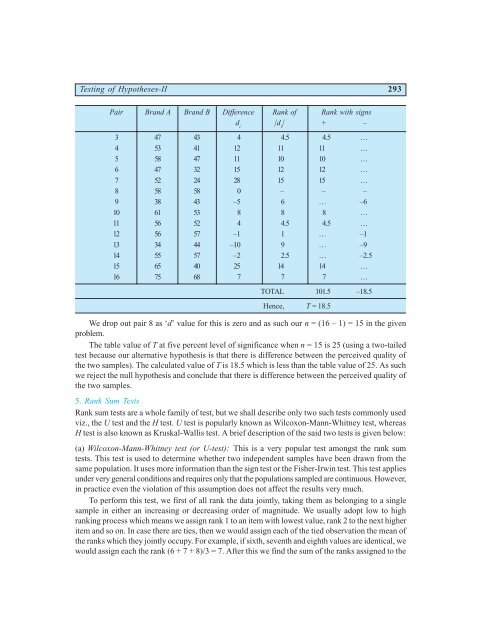
Testing of Hypotheses-II 293<br />
Pair Brand A Brand B Difference Rank of Rank with signs<br />
d i |d i | + –<br />
3 47 43 4 4.5 4.5 …<br />
4 53 41 12 11 11 …<br />
5 58 47 11 10 10 …<br />
6 47 32 15 12 12 …<br />
7 52 24 28 15 15 …<br />
8 58 58 0 – – –<br />
9 38 43 –5 6 … –6<br />
10 61 53 8 8 8 …<br />
11 56 52 4 4.5 4.5 …<br />
12 56 57 –1 1 … –1<br />
13 34 44 –10 9 … –9<br />
14 55 57 –2 2.5 … –2.5<br />
15 65 40 25 14 14 …<br />
16 75 68 7 7 7 …<br />
TOTAL 101.5 –18.5<br />
Hence, T = 18.5<br />
We drop out pair 8 as ‘d’ value for this is zero and as such our n = (16 – 1) = 15 in the given<br />
problem.<br />
The table value of T at five percent level of significance when n = 15 is 25 (using a two-tailed<br />
test because our alternative hypothesis is that there is difference between the perceived quality of<br />
the two samples). The calculated value of T is 18.5 which is less than the table value of 25. As such<br />
we reject the null hypothesis and conclude that there is difference between the perceived quality of<br />
the two samples.<br />
5. Rank Sum Tests<br />
Rank sum tests are a whole family of test, but we shall describe only two such tests commonly used<br />
viz., the U test and the H test. U test is popularly known as Wilcoxon-Mann-Whitney test, whereas<br />
H test is also known as Kruskal-Wallis test. A brief description of the said two tests is given below:<br />
(a) Wilcoxon-Mann-Whitney test (or U-test): This is a very popular test amongst the rank sum<br />
tests. This test is used to determine whether two independent samples have been drawn from the<br />
same population. It uses more information than the sign test or the Fisher-Irwin test. This test applies<br />
under very general conditions and requires only that the populations sampled are continuous. However,<br />
in practice even the violation of this assumption does not affect the results very much.<br />
To perform this test, we first of all rank the data jointly, taking them as belonging to a single<br />
sample in either an increasing or decreasing order of magnitude. We usually adopt low to high<br />
ranking process which means we assign rank 1 to an item with lowest value, rank 2 to the next higher<br />
item and so on. In case there are ties, then we would assign each of the tied observation the mean of<br />
the ranks which they jointly occupy. For example, if sixth, seventh and eighth values are identical, we<br />
would assign each the rank (6 + 7 + 8)/3 = 7. After this we find the sum of the ranks assigned to the


