Research Methodology - Dr. Krishan K. Pandey

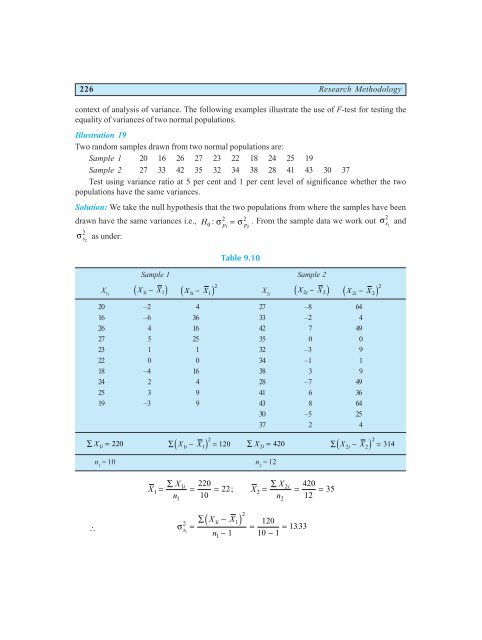
226 Research Methodology
context of analysis of variance. The following examples illustrate the use of F-test for testing the
equality of variances of two normal populations.
Illustration 19
Two random samples drawn from two normal populations are:
Sample 1 20 16 26 27 23 22 18 24 25 19
Sample 2 27 33 42 35 32 34 38 28 41 43 30 37
Test using variance ratio at 5 per cent and 1 per cent level of significance whether the two
populations have the same variances.
Solution: We take the null hypothesis that the two populations from where the samples have been
drawn have the same variances i.e., 2 2
2
H0: σ p = σ . From the sample data we work out σ
1 p
s1 and
2
2
σ s2 as under:
X 1i
Table 9.10
Sample 1 Sample 2
dX1i − X1i
X1i − X1
2
dX2i − X2i
X i − X
d i X 2i
2
d 2 2i
20 –2 4 27 –8 64
16 –6 36 33 –2 4
26 4 16 42 7 49
27 5 25 35 0 0
23 1 1 32 –3 9
22 0 0 34 –1 1
18 –4 16 38 3 9
24 2 4 28 –7 49
25 3 9 41 6 36
19 –3 9 43 8 64
30 –5 25
37 2 4
∑ X1i = 220 ∑ X − X =
2
d 1i 1i
120 ∑ X i =
n 1 = 10 n 2 = 12
X
1
X
=
n
∑
∴ σ s
1
220
X
= = 22 X 2 =
10
n
∑
;
1i
2i
d i .
2
X i X
2 1 1
=
1 n1
1
∑ −
−
2
d 2i 2i
2 420 ∑ X − X = 314
120
= 1333
10 − 1
=
2
420
= = 35
12