Research Methodology - Dr. Krishan K. Pandey

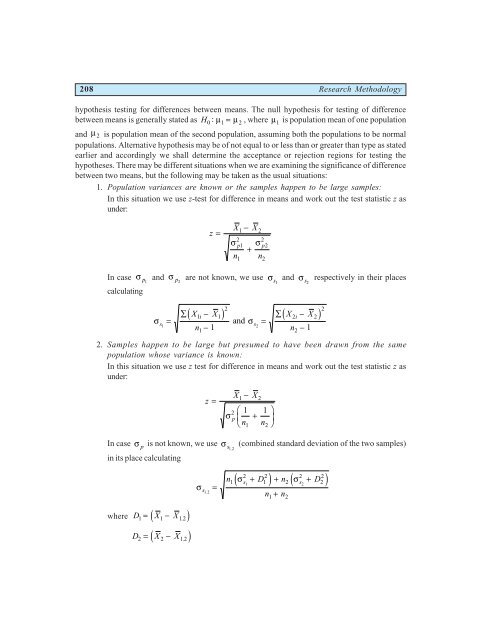
208 Research Methodology
hypothesis testing for differences between means. The null hypothesis for testing of difference
: μ = μ , where μ1 is population mean of one population
between means is generally stated as H 0 1 2
and μ 2 is population mean of the second population, assuming both the populations to be normal
populations. Alternative hypothesis may be of not equal to or less than or greater than type as stated
earlier and accordingly we shall determine the acceptance or rejection regions for testing the
hypotheses. There may be different situations when we are examining the significance of difference
between two means, but the following may be taken as the usual situations:
1. Population variances are known or the samples happen to be large samples:
In this situation we use z-test for difference in means and work out the test statistic z as
under:
z =
X − X
1 2
2 2
p p2
σ 1 σ
+
n n
1
In case σ p1 and σ p2 are not known, we use σ s1 and σ s2 respectively in their places
calculating
2
2
d i d 2 2i
X1i X1
X i X
σs = σ
1 s2
n 1 n 1
∑ −
=
−
∑ −
and
−
1
2. Samples happen to be large but presumed to have been drawn from the same
population whose variance is known:
In this situation we use z test for difference in means and work out the test statistic z as
under:
z =
In case σ p is not known, we use σ s12 .
in its place calculating
d i
d i
where D = X − X .
1 1 12
D = X − X .
2 2 12
σ
s
12
. =
σ
X − X
2
p
F
HG
1 2
2
1 1
+
n n
1 2
I
KJ
2
(combined standard deviation of the two samples)
2 2
2 2
1e
s1 1j
2e
s2
2j
n σ + D + n σ + D
n + n
1 2