OPRE 6366 : PROBLEM SESSION - The University of Texas at Dallas

OPRE 6366 : PROBLEM SESSION
QUESTIONS
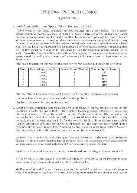
1. Web Mercentile Floor Space: Hillier Liberman p.95, 3.4-9.
Web Mercantile sells many household products through an on-line catalog. The company
needs substantial warehouse space for storing its goods. Plans now are being made for leasing
warehouse storage space over the next 5 months. Just how much space will be required in each
of these months is known. However, since these space requirements are quite different, it may
be most economical to lease only the amount needed each month on a month-by-month basis.
On the other hand, the additional cost for leasing space for additional months is much less than
for the first month, so it may be less expensive to lease the maximum amount needed for the
entire 5 months. Another option is the intermediate approach of changing the total amount of
space leased (by adding a new lease and/or having an old lease expire) at least once but not
every month.
The space requirement and the leasing costs for the various leasing periods are as follows:
Month Required Space (Sq. Ft.) Leasing Period (Months) Cost per Sq. Ft. Leased
1 30,000 1 $65
2 20,000 2 $100
3 40,000 3 $135
4 10,000 4 $160
5 50,000 5 $190
The objective is to minimize the total leasing cost for meeting the space requirements.
(a) Formulate a linear programming model for this problem.
(b) Solve this model by the simplex method.
2. Swort produces swimming suits for Dallas area sport teams. It has two production and storage
locations in South and North Dallas. The southern facility produces 100 suits per month and
the same number is 150 for the northern facility. Production costs are $22 per suit at the
former facility and $24 at the latter facility. It costs $2 to send suits from southern facility
to markets and the same number is $1 for the northern facility. Swort designs a new suit in
each November and sells only this suit to its customer until the next November. Swort splits a
year into two periods: Winter from November to March and Summer from April to October.
Keeping a single suit in the inventory from one period to the next costs $2.
a) Swort has a production cycle that goes from one November to the next, and production
during a cycle is planned independent of previous cycles. Is considering cycles independently
an approximation or an exact reflection of Swort’s business process. Explain.
b) What are the production capacities in the south and north during winter and summer?
c) Let W and S be suit demands in winter and summer. Formulate a Linear Program to minimize
production/transportation and inventory holding costs.
d) How small should S be such that no inventory is carried from winter to summer? Suppose
that S is sufficiently small and W = 900, how many units must be produced at each facility
1

during winter?
e) Aggregate Locations: Since southern and northern facilities have similar costs, you can
aggregate them into a single facility for planning purposes. Perform this aggregation with a
pessimistic point of view; Whenever you are to choose between two cost figures in aggregating
the south and the north into a single facility, choose the largest costs. This is worst case analysis.
After this aggregation production plan simplifies, how many units should be produced at
this single facility in the summer and the winter if W = 900 and S = 2000. What would be
the (minimum) cost of production/transportation and inventory, express this number do not
compute?
f) Disaggregate Locations: If you found the winter production to be 1000 units in f), how will
you distribute this to the south and the north?
2

3. Fixed charge transportation problem: Consider m suppliers and n customers where supplier i
ships to customer j at the cost of cij per unit. Supplier i has Si units of supply and customer
j has Dj units of demand. Unlike a standard transportation problem, links between suppliers
and customers have to be built at a cost of fij per link (i, j). The objective is to find out which
links to build as well as how much flow to send over the links such that sum of transportation
and link-building costs are minimized.
a) Provide a formulation to minimize total transportation and link-building costs.
b) Modify your formulation so that at least three links are built to connect each customer to
3 suppliers. Explain in 1 sentence why in practice one would use several links to supply to a
given customer as oppposed say only 1 or 2 links?
c) Refer to a). Suppose that travel over the link (i, j) takes tij time. Modify your formulation
of a) so that each link that you choose to build can transport materials from suppliers to customers
within T units of time.
d) Refer to a). Now suppose that you decide to be more customer oriented; you impose a
different timing limit Tj for each customer j, each link that you choose to build from suppliers
to customer j must transport within Tj units of time. Modify your formulation to c). Explain
in 1 sentence why a company in practice would use different Tj values for different customers.
e) Bottleneck time transportation problem: Suppose that you are planning transportation links
for US Navy for which transportation costs are not important but deployment times are. The
Navy wants to deploy from domestic bases to all of its overseas bases as soon as possible: It
wants to minimize the maximum transportation time from domestic bases to overseas bases but
only for the links you choose to build, formally
min (max{tij where link (i, j) is built})
First establish an anology in your mind between warehouses and domestic bases, and between
customers and overseas bases. Provide a formulation for this problem. Explain in 1 sentence
why this problem may be called bottleneck time transportation problem.
3

4. Capacity expansion under uncertainty: SAuto manufactures cars in USA (U) and Mexico (M)
with annual plant capacities of 60K and 30K cars. Cars produced in USA can be sold in USA
only, cars produced in Mexico can be sold in Mexico only. Currently annual SAuto car demand
is 70K and 30K in USA and Mexico. However, due to migration of people between these countries,
the car demand is equally likely to increase or decrease by 10K in each country in each
year in the following 2 years, we do not expect any uncertainty on top of the migration uncertainty.
Thus, demands in Mexico DM and US DU are perfectly negatively correlated in each
year: DM + DU = 100 K cars. We are considering whether to expand capacity by 20K units
and if so whether in Mexico or in US but not in both. For example, if capacity is expanded in
Mexico it goes up to 50K cars and then US capacity must stay constant at 60K cars. Expansion
costs are the same in both countries. We will choose the capacity now in year 0 and apply the
same capacity for the next 2 years, i.e. over a total of 3 years.
a) Let us index demands with a superscript to distunguish between years 0, 1 and 2. For
example, (D 0 U, D 0 M) = (70, 30) in year 0. Now suppose that we were told about events
(D 1 U, D 1 M) = (80, 20) and (D 2 U, D 2 M) = (50, 50). Explain what these events mean in English, can
(D 2 U, D 2 M) = (50, 50) happen after (D 1 U, D 1 M) = (80, 20), why?
b) Consider a scenario given as (D 0 U, D 0 M; D 1 U, D 1 M; D 2 U, D 2 M) = (70, 30; 80, 20; 70, 30), write in
English what this means. Write all possible scenarios and their probabilities of occurence. Also
discuss if capacity levels are nonanticapatory with respect to demands or not.
c) Suppose that SAuto chooses not to expand the capacity and keep it as (60, 30) draw a decision
tree and compute the product shortage in each country on each node of the decision tree.
Suppose that SAuto incurs shortage costs of sU in US and sM in Mexico, compute the expected
shortage cost from the tree for capacity (60, 30) in terms of sU and sM.
d) Repeat c) for capacity expansions in US only and in Mexico only.
e) Explain why would you make the expansion either in Mexico or US, if expansion is free.
Suppose that sU = 1. For what range of values of sM the investment should be made in Mexico?
f) Suppose that sU = 1 and sM = 2. For what range of values of the expansion cost the
expansion should be made and made in Mexico plant?
4

5. A typical aggregate planning problem over T = 6 months can be formulated with the parameters
and decision varaiables as below:
Rt = Number of workers in month t, t = 1, ..., 6. R0 = Starting number of workers in month
t = 1.
Ot = Number of overtime hours worked in month t, t = 1, ..., 6.
Nt = Number of new employees hired at the beginning of month t, t = 1, ..., 6.
Lt = Number of employees laid off at the beginning of month t, t = 1, ..., 6.
It = Inventory at the end of month t, t = 1, ..., 6. I0 = Starting inventory in month t = 1.
Bt = Number of products of backlog at the end of month t, t = 1, ..., 6. B0 = Starting level of
backlog in month t = 1.
Pt = Number of products produced in month t, t = 1, ..., 6.
St = Number of products subcontracted in month t, t = 1, ..., 6.
Dt = Number of products demanded in month t, t = 1, ..., 6.
r, o, n, l, i, b, p, s= cost of regular workers, overtime, new worker hiring, laying-off, inventory
holding, backlog cost, production cost, subcontract cost
h = Number of products produced by one worker in a month by working regular time.
e = Number of products produced by one worker in one hour of overtime.
a = Allowable number of overtime per regular worker per month based on labor regulations.
The formulation is:
Min � T 1 rRt + oOt + nNt + lLt + iIt + bBt + pPt + sSt
ST.
Rt = Rt−1 + Nt − Lt for t = 1 . . . T .
It = It−1 + Pt + St − Dt − Bt−1 + Bt for t = 1 . . . T .
Pt ≤ hRt + eOt
Ot ≤ aRt
All decision variables are nonnegative.
a) Is BtIt = 0, why?
b) The above formulation considers inventory at the end of a month to compute the inventory
holding cost. The management would like instead to use average inventory in each month
defined as the average of the starting and ending inventories in each month. How should the
management target for the ending inventory at the end of the sixth month so that this new
approach yield the same result as the above formulation?
c) Write a condition among s, o and e which guarantees that the overtime is less costly than
the subcontracting.
d) Suppose that the condition in c) fails. However, the workers’ union wants to enforce the
condition that no subcontracting can take place before all the overtime capacity is exploited.
Add a constraint to the original formulation to take this condition into account.
5

6. A Location Problem
It is desirable to locate service facilities physically close to where the demands are. Suppose
that there are only 4 existing apartment complexes in a small town and the coordinates of the
jth complex is given as (xj, yj) for j = 1..3. We want to locate a mall at a location (a, b) where
a, b are to be decided upon. The distance between the mall and the jth complex is given by
|a − xj| + |b − yj|. Provide an LP formulation to minimize the total rectilinear distance
between the mall and the apartments.
7. Manpower Planning: At the post office on the Coit street, each employee works exactly for
5 consecutive days per week. To provide a satisfactory customer service, the post office needs
the following number of employees each day:
Days Mon Tue Wed Thu Fri Sat Sun
# of employees required 9 6 5 8 11 13 4
a) Provide an LP formulation to minimize the number of employees.
b) Suppose some employees are willing to do overtime and work for one more day right after
their 5 day regular schedule. Suppose that overtime labor rate is 50% more than regular labor
rate. Provide an LP formulation to minimize the labor costs.
8. Consider Texas Nameplate, a metal nameplate company in Dallas, which produces nameplates
for equipment, exhibits, etc. Texas Nameplate works with a pull process where customers give
orders of Qi plates of type i and specify a due date of di for the deliveries. All plates of order i
must be delivered by the due date di. Suppose that there are n existing orders (1 ≤ i ≤ n) and
m days in the planning horizon (1 ≤ di ≤ m). Texas Nameplate has the production capacity
of c plates per day. Since the plates are similar enough, we prefer to deal with the aggregated
capacity.
Once Texas Nameplate finishes the production of the plates, it sends them b FedEx to the
customers. FedEx makes (m + 1) many delivery options available: 0-day (overnight) delivery,
1-day delivery, 2-day delivery, . . . , (m)-day delivery. Plates whose due dates are di must be
shipped by Texas Nameplate on day di by using overnight delivery. The cost of shipping one
plate on a j day delivery option is a − bj where a, b are constants such that a ≥ bm. Assume
that all customers accept partial shipments.
a) Suppose that n = 3, m = 2 and Q1 = Q2 = Q3 = 10, d1 = d2 = d3 = 2 and c = 20. In
order to minimize the delivery costs for Texas Nameplate, determine how many units should
be shipped on each day. Compute the cost of your shipment plan. This is such a small problem
that you can see the solution by inspection. Save your appetite for a formulation to part e).
b) This part is independent of a). Let qij be the number of nameplates produced on day j and
shipped to for customer order i. Suppose that m = 4 and the data for two orders are as follows:
q13 = 10, q24 = 20 and q14 = 10. Mark T or X before the following statements.
• ( ) c = 10.
• ( ) Q1 = 30.
6

c) This part is independent of a,b). Let us define Aj = {order i such that di ≤ j}. Aj is the set
of orders due on day j or earlier. Suppose that d1 = 7, d2 = 4, d3 = 6, d4 = 4, d5 = 3, d6 = 7.
Write only A1, A3, A5, A7.
d) When d1 = 1, Q1 = 30 and c = 20, customer order 1 cannot be finished on time. That is,
the problem is infeasible. Write a single inequality that involves only problem parameters such
that whenever the inequality holds, the problem is feasible. Your inequality must say that the
total number of name plates due by day j is less than or equal to the total production capacity
available in the first j days. You can use Aj’s defined in part c).
e) Write an LP to minimize the total shipment. List your decision variables first. You can use
qij defined early in your formulation.
f) Establish an analogy with the transportation problem. Draw a network with m nodes on the
left and m nodes on the right hand side. Think of each node as a time period. The nodes on
the left hand side are supply nodes and the nodes on the right hand side are demand nodes.
Now pose the problem as a transportation problem by defining supply (demand) quantity for
each supply (demand) node and the transportation cost cij from supply node i to demand node
j. Basically fill in the blanks below by using problem parameters: Qi, c, di, a and b.
9. A coworker of yours made a capacity expansion formulation for M type of machines and N
type of products over T months, with the following parameters:
dt,j: Number of product type j demanded in month t.
mj : Profit made by producing and selling a product j.
ci: Cost of purchasing a machine of type i.
and decision variables:
nt,i: Number of machines of type i purchased and installed in month t.
xt,j: Number of products of type j produced in month t.
Maximize
T� M�
T� N�
− cint,i + mjxt,j
t=1 i=1
t=1 j=1
Subject to
kt,i =
t�
nτ,i
τ=1
for t = 1 . . . T and i = 1 . . . M.
N�
ai,jxt,j ≤ 160kt,i for t = 1 . . . T and i = 1 . . . M.
j=1
xt,j ≤ dt,j for t = 1 . . . T and j = 1 . . . N.
xt,j ≥ 0 for t = 1 . . . T and j = 1 . . . N.
nt,i ≥ 0, int i.e., nonnegative integer for t = 1 . . . T and i = 1 . . . M.
where 160 is the number of hours a machine works in a month.
a) Express kt,i and ai,j in English and write their units.
b) The formulation does not include inventories. Is it more appropriate for a manufacturing or
a service company?
7

c) The formulation above is flawed. To see this, set nt,i = 0 for each month t ≥ 2. Explain to
your coworker in English what these restrictions mean and why they do not affect the formulation.
d) Your coworker is convinced with your explanation in part c). To save his face, he has just
remembered that he forgot to include a machine maintenance cost of bi per month for each i
type machine. Help him to include this cost appropriately in the formulation.
e) Losing confidence in your coworker in part c) and getting involved in the formulation in
part d) have awakened your insatiable curiosity. You question your coworker about machine
purchase / installation lead times and demand uncertainty. Your coworker says:
“- Almost all of our customers finalize their orders a month before their purchase. Thus, looking
one month ahead we have virtually certain demands, so we work with at least 1 month of frozen
horizon. However, demands carry substantial uncertainty 4-5 months before their occurrence
but our flexible horizon starts before the 4. month into the future. On the other hand, we always
buy our machines from the same vendor which requires that we order machines 6 months in
advance for their timely production and installation. I think that machine purchase and installation
lead times are 6 months.”
In light of this conversation, determine if demand uncertainty needs to be taken into account
for capacity expansion. Suppose that you will treat demand uncertainty with L equally likely
demand scenarios. Identify anticipatory and nonanticipataory variables. Given the 6 months of
purchase and installation lead time, can the formulation be pertaining to the next 1-6 months
from the current month?
f) Recalling that anticipatory variables can be scenario specific, provide a formulation by introducing
L scenarios appropriately into the correct formulation in d).
g) If the machine purchase/installation lead time is decreased to 1 month from 6 months, do
you expect a better objective function value, why?
8

SOLUTIONS
1. Web Mercentile Floor Space: Put solution of Hillier Liberman p.95, 3.4-9.
(a) Let xij = the amount of space leased in month i for a period of j months for i = 1, ..., 5 and
j = 1, ..., 6 − i.
Minimize C = 650(x11 + x21 + x31 + x41 + x51) + 1000(x12 + x22 + x32 + x42)
+1350(x13 + x23 + x33) + 1600(x14 + x24) + 1900x15
subject to x11 + x12 + x13 + x14 + x15 ≥ 30, 000
x12 + x13 + x14 + x15 + x21 + x22 + x23 + x24 ≥ 20, 000
x13 + x14 + x15 + x22 + x23 + x24 + x31 + x32 + x33 ≥ 40, 000
x14 + x15 + x23 + x24 + x32 + x33 + x41 + x42 ≥ 10, 000
x15 + x24 + x33 + x42 + x51 ≥ 50, 000
and xij ≥ 0, fori = 1, ..., 5 and j = 1, ..., 6 − i.
2. a) Cycles can be considered independently because every cycle starts with a new product (new
design).
b) Northern capacities are 750 and 1050 in the winter and the summer. Southern capacities
are 500 and 700 in the winter and the summer.
c) Let W NW be the Winter production made at the North for Winter demand. Define W SW ,
W NS, W SS, SNS and SSS.
Min 25W NW + 24W SW + 27W NS + 26W SS + 25SNS + 24SSS
ST:
W NW + W NS ≤ 750
W SW + W SS ≤ 500
SNS ≤ 1050
SSS ≤ 700
W NW + W SW ≥ W
W NS + W SS + SNS + SSS ≥ S
W NW, W SW, W NS, W SS, SNS, SSS ≥ 0
Note that this is nothing but a transportation problem.
d) Since it costs less to produce in summer and serve the summer demand, as long as S ≤ 1750
there will be no need to keep inventory for the summer. The cheapest way to meet the winter
demand of 900 is to produce 500 at the southern facility and 400 at the northern facility.
e) Worst case analysis dictates that we use northern (expansive) facility’s costs. We produce
1150 units in the winter, use 9000 for the winter demand and keep 250 for the summer. In the
summer we produce 1750 units and use them with the inventory of 250 to satisfy the demand
of 2000. The minimum cost is: (25)900+(27)250+(25)1750.
f) First fill up the cheapest (south) then move to the other location (north): Produce 500 at
the south and another 500 at the north.
In summary, this problem allows you to exercise with time-wise and location-wise aggregation
and desegregation in the context of production and inventory using a transportation problem
formulation.
9

3. a) Let xij be the flow on arc (i, j). Let yij = 1 if arc (i, j) is built.
Min �m �nj=1 i=1 cijxij + �m �nj=1 i=1 fijyij
ST:
�mi=1 xij ≥ Dj for all customer j
�nj=1 xij ≤ Si for all supplier i
xij ≤ Siyij for all arcs (i, j)
xij ≥ 0 and yij ∈ {0, 1}
b) Add the constrant � m i=1 yij ≥ 3 for all customer j. Several links are used to supply the
customer in case one or two links fail or corresponding suppliers do not have enough inventory.
This is the idea behind dual/triple sourcing.
c) Add tijyij ≤ T for i = 1..m and j = 1..n. Note that tij are data so formulation is linear.
d) Add yijtij ≤ Tj for i = 1..m and j = 1..n. Different Tj values for different customers provide
delivery time customization.
e) Replace the objective with Min t and add the constraints:
t ≥ yijtij for i = 1..m and j = 1..n.
t is the maximum transportation time from suppliers to customers so it is the bottleneck time.
4. a) (D 1 U, D 1 M) = (80, 20) implies demands are 80K and 20K in US and Mexico in year 1.
(D 2 U, D 2 M) = (50, 50) implies demands are 50K and 50K in US and Mexico in year 2.
(D 2 U, D 2 M) = (50, 50) cannot happen after (D 1 U, D 1 M) = (80, 20) because demand varies only by
10K.
b) (D 0 U, D 0 M; D 1 U, D 1 M; D 2 U, D 2 M) = (70, 30; 80, 20; 70, 30) implies 70K and 30K demand in US
and Mexico in year 0; 80K and 20K demand in US and Mexico in year 1; 70K and 30K demand
in US and Mexico in year 2.
All scenarios: (70,30; 80,20; 90,10); (70,30; 80,20; 70,30); (70,30; 60,40; 70,30); (70,30; 60,40;
50,50).
Capacty is determined before the demands occur so it must be nonanticapatory.
c) Expected shortage cost=10sU +(0.5)20sU +(0.5)10sM +(0.25)30sU +(0.5)10sU +(0.25)20sM =
65sU/2 + 10sM
d) With US expansion: Expected shortage cost=(0.5)10sM +(0.25)10sU +(0.25)20sM = 5sU/2+
10sM.
With Mexico expansion: Expected shortage cost=10sU + (0.5)20sU + (0.25)30sU + (0.5)10sU =
65sU/2
e) With expansion shortage costs decrease so it must be made either in Mexico or US. Expansion
is made in Mexico if shortage costs with Mexico expansion is smaller: 65sU/2 ≤ 5sU/2 + 10sM
inserting sU = 1 yields sM ≥ 3.
Need Expected shortage cost=5sU/2+10sM ≥ 65sU/2=Expected shortage cost implies sM ≥ 3.
f) Need expansion cost M such that M + 65/2 ≤ min{65/2 + 20, M + 5/2 + 20}. No M value
satisfies this inequality. Indeed, if M ≤ 20 expand US plant. Otherwise do not expand at all.
10

Year 0
(70,30)
(60,30)
(10,00)
Legend:
(USDem , MexDem)
(USCap , MexCap)
(USShort , MexShort)
Year 0
(70,30)
(80,30)
(00,00)
Legend:
(USDem , MexDem)
(USCap , MexCap)
(USShort , MexShort)
Year 1
(80,20)
(60,30)
(20,00)
(60,40)
(60,30)
(00,10)
Year 1
(80,20)
(80,30)
(00,00)
(60,40)
(80,30)
(00,10)
Year 2
(90,10)
(60,30)
(30,00)
(70,30)
(60,30)
(10,00)
(50,50)
(60,30)
(00,20)
Year 2
(90,10)
(80,30)
(10,00)
(70,30)
(80,30)
(00,00)
(50,50)
(80,30)
(00,20)
5. a) Yes. By definition if there is backlog, it means there is no excess inventory. And if there is
inventory it will be used up to meet the backlog.
b) In the new formulation we replace i � T t=1 It with i � T t=1
i
T�
t=1
It−1 + It
2
= i I0 + IT
2
T� −1
+ i
t=1
It−1+It
2
It = i I0 − IT
2
Then we obtain the same result when IT is set equal to I0.
where
T�
+ i It
t=1
c) Need subcontracting cost per unit larger than the overtime cost per unit: s ≥ o/e.
d) Need two constraints: � T t=1(h · Rt + e · Ot) − � T t=1 Dt ≤ ( � T t=1 Dt)(1 − y) and � T t=1 St ≤
( � T t=1 Dt)y.
11

Year 0
(70,30)
(60,50)
(10,00)
Legend:
(USDem , MexDem)
(USCap , MexCap)
(USShort , MexShort)
Year 1
(80,20)
(60,50)
(20,00)
(60,40)
(60,50)
(00,00)
Year 2
(90,10)
(60,50)
(30,00)
(70,30)
(60,50)
(10,00)
(50,50)
(60,50)
(00,00)
The left hand side is the excess production capacity in number of units over T months. If the
excess capacity is positive then y = 0. That is subcontracting cannot be used, which is implied
by the second constraint. If the excess capacity is negative or zero, the first constraint does not
imply anything about y.
6. 1. Decision Variables
We are deciding on the coordinates of the mall specified by (a, b): a, b are decision variables.
Let d x j be the x component of the rectilinear distance between the mall and the complex j.
Define d y
j similarly for y components.
2. Objective Function
3. Constraints
Mind x 1 + d x 2 + d x 3 + d y
1 + d y
2 + d y
3
d x 1 = |a − x1| =⇒ d x 1 = max{a − x1, −(a − x1)}.
d x 1 = max{a − x1, −(a − x1)} =⇒ d x 1 ≥ a − x1 and d x 1 ≥ −(a − x1).
Then in the optimal solution:
d x 1 ≥ a − x1 and d x 1 ≥ −(a − x1) Min dx 1 +...
=⇒ d x 1 = a − x1 or d x 1 = −(a − x1)
Thus, d x 1 = |a − x1| is satisfied by the optimal solution. No more constraints on d x 1.
12

4. Remarks
Min d x 1 + d x 2 + d x 3 + d y
1 + d y
2 + d y
3
Subject to:
d x j ≥ a − xj j = 1, 2, 3
d x j ≥ −(a − xj) j = 1, 2, 3
d y
j ≥ b − yj j = 1, 2, 3
d y
j ≥ −(b − yj) j = 1, 2, 3
(a) Do we need nonnegativity constraints on d x j or d y
j ?
(b) Suppose that the first apartment complex has twice as many people as others. How do we
modify the formulation?
(c) When the objective function is the (population) weighted sum of distances, it represents
a private sector objective. When p facilities are to be located, the problem is called the
p-Median problem.
(d) Suppose that we are locating a fire station (as opposed to a mall) and we want to minimize
the maximum of the distances between the station and the apartments, i.e. min {max {|a−
xj| + |b − yj| , j = 1..3}}. How do we modify the formulation?
(e) When the objective function is minimizing the distance to the furthest apartment complex,
it represents a public sector objective. When p facilities are to be located, the problem is
called the p-Center problem.
7. Let xi= the number of employees hired to start working in day i ( i=1, 2,...,7 )
a) Min (x1 + x2 + x3 + x4 + x5 + x6 + x7)
s.t. (number of employees available in each day)
x1 + x4 + x5 + x6 + x7 ≥ 9
x1 + x2 + x5 + x6 + x7 ≥ 6
x1 + x2 + x3 + x6 + x7 ≥ 5
x1 + x2 + x3 + x4 + x7 ≥ 8
x1 + x2 + x3 + x4 + x5 ≥ 11
x2 + x3 + x4 + x5 + x6 ≥ 13
x3 + x4 + x5 + x6 + x7 ≥ 4
xi ≥ 0 ( i = 1...7 )
b) Let xi = the number of employees hired to start working in day i ( i=1, 2, ...,7 )
Let x ∗ i = the number of employees hired to start working in day i and doing overtime for one
more day ( i=1,2,...,7 )
**Suppose that daily labor rate for an employee is ”1” unit. So each employee working in
regular days (5 days) has a cost of ”5”. When it does overtime, his cost is ”1.5”
Min 5*(x1 + x2 + x3 + x4 + x5 + x6 + x7)+1.5*(x ∗ 1 + x ∗ 2 + x ∗ 3 + x ∗ 4 + x ∗ 5 + x ∗ 6 + x ∗ 7)
s.t. ( number of employees available in each day)
x1 + x4 + x5 + x6 + x7 + x ∗ 3 ≥ 9
x1 + x2 + x5 + x6 + x7 + x ∗ 4 ≥ 6
x1 + x2 + x3 + x6 + x7 + x ∗ 5 ≥ 5
x1 + x2 + x3 + x4 + x7 + x ∗ 6 ≥ 8
x1 + x2 + x3 + x4 + x5 + x ∗ 7 ≥ 11
x2 + x3 + x4 + x5 + x6 + x ∗ 1 ≥ 13
13

x3 + x4 + x5 + x6 + x7 + x ∗ 2 ≥ 4
xi ≥ x ∗ i
xi, x ∗ i ≥ 0 ( i = 1...7 )
8. a) Send 20 for Q1 and Q2 on the first day and Q3 on the third day. Cost is 20(a−1.b)+10(a−0.b).
b) ( X ) c = 10.
( X ) Q1 = 30.
c) A1 = ∅, A3 = {5}, A5 = {2, 4, 5}, A7 = {1, 2, 3, 4, 5, 6}.
d)
�
Qi ≤ cj.
i∈Aj
e) qij, defined in b), is the decision variable.
Minimize �n �di i=1 j=1(b − a(di − j))qij
Subject to
�di j=1 qij = Qi i = 1, . . . , n
�ni=1 qij ≤ c j = 1, . . . , di
qij ≥ 0
f) Supply for supply node i (day i) = c
Demand for demand node j (day j) = �
{i:di=j} Qi or say sum of the customer orders due to
day j.
Transportation cost ci,j per unit = a − b(j − i) if j ≥ i. Cost is infinite if j < i.
9. a) kt,i: Number of machines installed by month j, units in numbers. ai,j: Machine type i hours
required to produce a product of type j, units in hours.
b) Service company.
c) The restrictions imply that no purchases can be made after the first month. Restrictions do
not affect the formulation because as many as necessary machines can still be purchased in the
first month without violating constraints and changing the objective value. Basically, formulation
is flawed because any machine purchased in month t can be purchased earlier without
altering anything in the formulation. This is fixed in part d) below.
Formally, suppose that n ∗ t,i are the optimal solution without the restrictions. With the restric-
tions buy �
t n ∗ t,i in the first month and nothing afterwards. You get the same optimal objective
value.
d) Add �
�
t
� t
i bikt,i.
�
i(T − t)bint,i to the objective function. Alternative but equivalent answer is
14

e) Demand uncertainty is substantial at time of ordering for machines so it needs to be taken
into account for capacity expansion. nonanticipatory variables: nt,i. Anticipatory variabels:
xt,j.
The capacity formulation must deal with months at least 6 month from the current month.
f) Define scenario specific variables x l t,j:
Maximize
T� M�
− cint,i +
t=1 i=1
1
L� T� N�
mjx
L l=1 t=1 j=1
l Subject to
T� M�
t,j − (T − t)bint,i
t=1 i=1
kt,i =
t�
nτ,i
τ=1
for t = 1 . . . T and i = 1 . . . M.
N�
aj,ix l t,j ≤ 160kt,i for t = 1 . . . T , i = 1 . . . M and l = 1 . . . L.
j=1
x l t,j ≤ d l t,j for t = 1 . . . T , j = 1 . . . N and l = 1 . . . L.
x l t,j ≥ 0 for t = 1 . . . T , j = 1 . . . N and l = 1 . . . L.
nt,i ≥ 0, int i.e., nonnegative integer for t = 1 . . . T and i = 1 . . . M.
g) A higher objective value can be achieved because nt,i can be anticipatory and assume a
different value in each scenario. This will give a relaxation of the constraints involving nt,i in
f).
15