Journal of Computers - Academy Publisher

More documents

Recommendations

Info

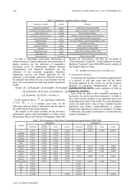
1828 JOURNAL OF COMPUTERS, VOL. 6, NO. 9, SEPTEMBER 2011 Table 2: Explanatory variables and their settings Explanatory variables Symbol Meaning Agriculture endowment agrgift Added value of agriculture/GDP Endowment of natural resources natgift Output of extractive industries/GDP Capital endowment capgift Rate of capital formation Endowment of human resources humgift Number of students in higher school/Population Level of urbanization city Urban employment/Total employment Market demand demand Provincial GDP per capita/National GDP per capita Transportation road Classified road density Industrial foundation industry Added value of industry /GDP Openness open Foreign direct investment/GDP Supporting services service Added value of tertiary industry /GDP Patent approvals patent Provincial patent approvals/National patent approvals Financial income fisc-income Financial income/GDP In table 2, Agriculture endowment, Endowment of natural resources, Capital endowment and Endowment of human resources are the indicators of comparative advantage; Level of urbanization, Market demand, Transportation and Industrial foundation are the indicators of new economic geography; Openness, Supporting services and Patent approvals are the indicators of knowledge spillovers; Financial income is the indicator that reflect the role of government. On this basis, We recommend the following double logarithmic model: ln LQ = β0 + β1 ln agrgift + β2 ln natgift + β3 ln capgift + β6 ln demand + β7 ln road + β8 lnindustry + β9 + β11 ln patent + β12 ln fisc − income + ε β In the equation above, i are regression coefficient, i = 1, 2, ⋅⋅ ⋅30, ε is a random error term. In the following empirical analysis, adjustment may be made to the model based on the actual situation. The sample in this paper includes all the provinces, autonomous regions and municipalities in China except Hong Kong, Macao and Taiwan (Chongqing is taken into Sichuan for convenience). All data can be found in "China Statistical Yearbook", "China Industrial Economy Statistical Yearbook" from 2000-2009 and the website of The People's Bank of China. IV. EMPIRICAL ESTIMATION AND RESULTS A. Econometric Analysis Considering the formation of industrial agglomeration is a process, it will take some time for the effect becoming apparent. In this article, we set the Location Quotient of provincial Manufacturing of 2008 as + dependent β4 ln humgift variable + β5 ln and city the twelve indicators of 2006 as lnexplanatory open + β variables. 10 ln service ( 7) First of all, we make a OLS estimation including all the factors. As can be seen from estimation 1 of table 3, the t value of most variables is not significant and severe multicollinearity exists in the model. So some adjustment need to be made until t value of most variables become significant and model’s multicollinearity is weaken. Results after adjustment is shown in estimation 2 of table 3. Obviously, the model of estimation 2 is better than the model of estimation 1. Table 3: OLS estimation of the factors of manufacturing agglomeration (2006-2008) estimation 1 estimation 2 Variables Coefficient Standard deviation t value p value Coefficient Standard deviation t value p value C 1.0524 2.1146 0.4976 0.6250 1.5389 0.5981 2.5728 0.0166 lnagrgift -0.2014 0.2413 -0.8345 0.4155 lnnatgift -0.0147 0.0641 -0.2294 0.8212 lncapgift 0.3917 0.3991 0.9814 0.3401 lnhumgift -0.0791 0.2610 -0.3031 0.7654 lncity 0.2485 0.3863 0.6432 0.5286 lndemand 0.2833 0.4734 0.5984 0.5574 0.8064 0.1133 7.1131 0.0000 lnroad 0.1051 0.1081 0.9720 0.3446 0.0898 0.0522 1.7205 0.0982 lnindustry 1.2566 0.4098 3.0661 0.0069 1.3435 0.2508 5.3550 0.0000 lnopen 0.0744 0.0769 0.9678 0.3466 lnservice 1.1140 0.8528 1.3062 0.2088 1.3270 0.6093 2.1779 0.0394 lnpatent 0.0852 0.0849 1.0029 0.3299 lnfisc-income -0.5922 0.3889 -1.5228 0.1461 -0.3536 0.2448 -1.4441 0.1616 R 2 0.8936 0.9142 LogL 6.6697 4.7362 AIC 12.6606 2.5274 SC 30.8761 10.9347 F 21.3008 0.0000 62.8634 0.0000 © 2011 ACADEMY PUBLISHER
JOURNAL OF COMPUTERS, VOL. 6, NO. 9, SEPTEMBER 2011 1829 As can be seen from the above analysis, the main factors that influence China’s provincial manufacturing agglomeration include Market demand, Transportation, Industrial foundation, Supporting services and Financial income. Industrial foundation and Supporting services have positive impact on manufacturing agglomeration. Their elasticities are 1.3435 and 1.3270. While Financial income has a negative impact on manufacturing agglomeration with its elasticity -0.3536. Due to the fault of OLS method dealing with spatial autocorrelation, we intend to use spatial econometric models to analyze the influencing factors of manufacturing agglomeration. The new model is the one in estimation 2 of table 3: ln LQ = β0 + β1 ln demand + β2 ln road + β3 ln + β4 ln service + β5 ln fisc − income + ε We need to verify the existence of spatial autocorrelation before peforming spatial econometric analysis. The result of spatial dependence test is shown in table 4. Table 4: Spatial dependence test Spatial dependence MI/DF Statistics p value Moran’s I (Error) 0.1047 1.9679 0.0489 LMLAG 1 0.2102 0.6465 R-LMLAG 1 0.4540 0.5003 LMERR 1 0.0931 0.7602 R-LMERR 1 0.3370 0.5615 LM-SARMA 2 0.5472 0.7606 As is shown in table 4, LMERR, LMLAG, R-LMERR and R-LMLAG do not pass the test at significance level of 5%. And SEM is better comparing the value of LogL, industry AIC, SC and LR of SLM and SEM. The result of estimation of SLM and SEM ( 8) is displayed in table 5. Table 5: SLM and SEM estimation of the factors of manufacturing agglomeration (2006-2008) SLM SEM Variables β Standard deviation t value p value β Standard deviation t value p value C 1.6128 0.5600 2.8797 0.0039 1.5984 0.5300 3.0154 0.0025 lndemand 0.7757 0.1192 6.5054 0.0000 0.8018 0.0975 8.2223 0.0000 lnroad 0.0742 0.0573 1.2952 0.1952 0.0851 0.0437 1.9457 0.0516 lnindustry 1.3642 0.2306 5.9145 0.0000 1.3741 0.2224 6.1785 0.0000 lnservice 1.3462 0.5464 2.4635 0.0137 1.3585 0.5442 2.4960 0.0125 lnfisc-income 0.3370 0.2200 1.5319 0.1255 0.3516 0.2199 1.5985 0.1099 ρ/λ 0.0621 0.1208 0.5146 0.6067 0.3324 0.1275 2.6064 0.0074 Statistical test DF Statistics p value DF Statistics p value R 2 0.9296 0.9495 LogL 4.8505 4.8034 AIC 4.2989 2.3930 SC 14.1073 10.8002 LR 1 0.2285 0.6325 1 0.1344 0.7138 As is shown in table 5, the coefficients of all variables are positive. It indicate that this estimation is more consistent with theoretical analysis. Industrial foundation and Supporting services have positive impact on manufacturing agglomeration. Their elasticities are 1.3642 and 1.3462 in SLM, 1.3741 and 1.3585 in SEM. B. Prediction of Location Quotient of China’s Provincial Manufacturing BP neural network is error back propagation neural network and feedforward network. It is widely used in function approximation, pattern recognition and data compression. In this article, we will predict the 2009’s Location Quotient of China’s Provincial Manufacturing using Neural Network Toolbox in Matlab (2006, 2007 and 2008’s location quotient are references for comparison). The Matlab program of prediction is as follows (take Beijing for example): clc close all clear all p0=[2.4289 2.1880 2.0585 1.6110 1.3667 1.4216 1.4169 1.3470 1.2994 1.3316]; day=1999:2008; plot(day, p0,'b+') © 2011 ACADEMY PUBLISHER hold on plot(day, p0, 'r-.') p1=(p0-min(p0))./(max(p0)-min(p0)); for i=1:5; p(:,i)=p1(i:i+2); t(:,i)=p1(i+3); end p; t; for i=1:5; testp(:,i)=p1(i+1:i+3); testt(:,i)=p1(i+4); end net=newff(minmax(p),[20,1],{'logsig','purelin'},'trainl m'); net.trainParam.lr=0.8; net.trainParam.epochs = 500; net.trainParam.goal = 0.001; net=train(net,p,t); y=sim(net,testp); E=testt-y;
Page 1 and 2: Journal of Computers ISSN 1796-203X
Page 3: Research on Self-built Digital Reso
Page 6 and 7: 1798 JOURNAL OF COMPUTERS, VOL. 6,
Page 86 and 87:
1878 JOURNAL OF COMPUTERS, VOL. 6,
Page 88 and 89:
Page 90 and 91:
Page 92 and 93:
Page 94 and 95:
Page 96 and 97:
Page 98 and 99:
Page 100 and 101:
Page 102 and 103:
Page 104 and 105:
Page 106 and 107:
Page 108 and 109:
Page 110 and 111:
Page 112 and 113:
Page 114 and 115:
Page 116 and 117:
Page 118 and 119:
Page 120 and 121:
Page 122 and 123:
Page 124 and 125:
Page 126 and 127:
Page 128 and 129:
Page 130 and 131:
Page 132 and 133:
Page 134 and 135:
Page 136 and 137:
Page 138 and 139:
Page 140 and 141:
Page 142 and 143:
Page 144 and 145:
Page 146 and 147:
Page 148 and 149:
Page 150 and 151:
Page 152 and 153:
Page 154 and 155:
Page 156 and 157:
Page 158 and 159:
Page 160 and 161:
Page 162 and 163:
Page 164 and 165:
Page 166 and 167:
Page 168 and 169:
Page 170 and 171:
Page 172 and 173:
Page 174 and 175:
Page 176 and 177:
Page 178 and 179:
Page 180 and 181:
Page 182 and 183:
Page 184 and 185:
Page 186 and 187:
Page 188 and 189:
Page 190 and 191:
Page 192 and 193:
Page 194 and 195:
Page 196 and 197:
Page 198 and 199:
Page 200 and 201:
Page 202 and 203:
Page 204 and 205:
Page 206 and 207:
Page 208 and 209:
Page 211 and 212:
A Modified Technique for Analysis o
show all

Journal of Computers - Academy Publisher

Create successful ePaper yourself

Delete template?

Save as template?