Manual VIII - Methods for Projections of Urban and ... - Development

Department ofEconomic and Social Affairs
POPULATION STUDIES, No. 55
Manuals on methods of estimating population
MANUAL VIII
Methods for Projections
ofUrban and Rural Population
United Nations
New York, .1974

NOTE
Symbols of United Nations documents are composed of capital letters combined
with figures. Mention of such a symbol indicates a reference to a United Nations
document.
The designations employed and the presentation of the material in this publication
do not imply the expression of any opinion whatsoever on the part of the
Secretariat of the United Nations concerning the legal status of any country or
territory or of its authorities, or concerning the delimitation of its frontiers.
Population Studies Nos. I to 54 were issued under the series symbol ST/SOA/
Series AfI-54.
ST/ESA/SER.A/55
UNITED NAnONS PUBLICAnON
Sales No. E.74'xm.3
Price: $U.S. 7.00
(or equivalent in other currencies)

Pursuant to the recommendations of the Population
Commission, the United Nations Secretariat has been
preparing several manuals describing methods of demographic
analysis, estimation and projection needed for
economic and social policy purposes and suitable for use
in many countries, including those where demographic
statistics and methods of analysis are not yet well advanced.
Some of those manuals deal with the analysis and
evaluation of basic statistics, notably those of population
censuses, and others are concerned with the projection
of various population quantities which are needed in
diverse fields of economic and social planning. This
manual, concerned with the projection of urban and rural
population, is part of this longer-range programme.
The following manuals have been published so far in
the Manuals on Methods of Estimating Population series:
Manual I: Methods of Estimating Total Population for
Current Dates; 1
Manual II: Methods of Appraisal of Quality of Basic
Data for Population Estimates .. 2
Manual III: Methods for Population Projections by
Sex and Age; 3
Manual IV: Methods of Estimating Basic Demographic
Measures from Incomplete Data; 4
Manual V: Methods of Projecting the Economically
Active Population" 6
Manual VI: Methods ofMeasuring Internal Migration; 6
Manual VII: Methods of Projecting Households and
Families: 7 and, related to this series,
Methods of Analysing Census Data on Economic
Activities of the Population. 8
1 United Nations publication, Sales No. S2Xrn.5.
2 United Nations publication, Sales No. S6Xrn.2.
3 United Nations publication, Sales No. S6XIII.3.
4 United Nations publication, Sales No. 67XIII.2.
5 United Nations publication, Sales No. E.70XIII.2 (in cooperation
with the ILO).
6 United Nations publication, Sales No. E.70XIII.3.
7 United Nations publication, Sales No. 73Xrn.2.
8 United Nations publication, Sales No. E.69.XIII.2.
FOREWORD
iii
Also, within the context of this coherent and cumulative
programme, two other publications should be mentioned;
namely, Estimating Future School Enrolment in Developing
Countries, a Manual of Methodology, published
jointly by the United Nations and UNESCO, 9 and a
technical report entitled The Concept ofa Stable Population:
Application to the Study of Populations of Countries
with Incomplete Demographic Statistics.i" which presents
the theoretical background of part of the aforementioned
Manual IV.
In this manual, projections of urban and rural population
are dealt with on the assumption that methods of
projection of a country's total population, or its total
population by groups of sex and age, are already known,
and that such projections have in fact already been
carried out. Those methods have been dealt with in
Manual III of the present series. It is also assumed here
that the reader is somewhat familiar with the appraisal
of accuracy in basic statistics, a subject developed at
some length in the previous Manual II.
This manual has been drawn up especially with a view
to its uses in less developed countries or countries whose
population statistics are not very detailed. It is addressed
mainly to population analysts possessing limited technical
means, and it does not consider the possible uses of
computer methodology. The methods are accordingly
simple, but, depending on opportunities, may be elaborated
further.
The United Nations is indebted to the Demographic
Research and Training Centre (CELADE) in Santiago,
Chile; the United States Bureau of the Census; K. V.
Ramachandran of the Regional Institute for Population
Studies in Accra, Ghana; and D. Courgeau of the
Institut National d'Etudes Demographiques in Paris for
their review of the draft of this manual, and the many
useful suggestions which have been incorporated in its
final version.
9 United Nations publication, Sales No. 66XIII.3.
10 United Nations publication, Sales No. 6SXIII.3.

INTRODUCTION
CONTENTS
Page
1
Chapter
I. PROBLEMS OF DEFINITION OF URBAN POPULATION ...............•........ 9
Administrative definition: type of local government . . . . . . . . . . . . . . . . . . . . . . 9
Administrative definition: seats of district government. . . . .. . . .. . . .. .. .. .. 10
Definition by size of administrative units .. . . . . . . . . . . . . . . . . . . . . . . . . . . . . 10
Economic definition, applied to administrative units . . . . . . . . . . . . . . . . . . . . 11
Geographic definition: agglomerations . . . . . . . . . . . . . . . . . . . . . . . . . . . . . . . . 11
Geographic definition: metropolitan areas 12
Other definitions 12
Purposes served by various definitions . . . . . . . . . . . . . . . . . . . . . . . . . . . . . . . . . . 13
II. COMPONENTS OF URBAN AND RURAL POPULATION CHANGE 14
Differences between urban and rural sex-age structures 14
Urban residence ratios by sex and age. . . . . . . . . . . . . . . . . . . . . . . . . . . . . . . . . . 14
Differences between urban and rural crude death rates '" . . . . . . . . . . . . . . . 16
Differences between urban and rural crude birth rates. . . . . . . . . . . . . . . . . . . . 18
Differences between urban and rural rates of natural increase 18
Differences due to the effects of international migration 19
Differences due to internal rural-to-urban migration . . . . . . . . . . . . . . . . . . . . 19
Effects of rural-to-urban area reclassification .. . . . . . . . . . . . . . . . . . . . . . . . . . . 20
Net rural-to-urban population transfers, i.e. combined effects of migration
and area reclassification 21
Implications for projection methodology . . . . . . . . . . . . . . . . . . . . . . . . . . . . . . 23
III. TEMPO OF URBANIZATION AND URBAN CONCENTRATION 25
General considerations 25
Concept of a growth rate 25
Tempo of urbanization 26
Reasons for use of the urban-rural growth differenceas a measure of the tempo
of urbanization . . . . . . . . . . . . . . . . . . . . . . . . . . . . . . . . . . . . . . . . . . . . . . . . . . 27
Tempo of urban concentration 30
IV. PROJECTION OF URBAN AND RURAL POPULATION TOTALS USING THE SIMPLEST
METHODS 32
Use of urban growth rates. . . . . . . . . . . . . . . . . . . . . . . . . . . . . . . . . . . . . . . . . . . . 32
Use of rural growth rates 33
Ratio method 34
Summary 35
V. UNITED NATIONS METHOD OF URBAN AND RURAL POPULATION PROJECTIONS. 36
Actual observations concerning urban-rural growth differences. . . . . . . . . . . . 36
Formula for iterative calculation 38
Year-to-year interpolation of a five-yearly projection 38
Applications of the method (by annual rates) . . . . . . . . . . . . . . . . . . . . . . . . . . 38
v

Chapter Page
Same method, using exponential rates . . . . . . . . . . . . . . . . . . . . . . . . . . . . . . . . . . 42
Flexible assumptions 43
VI. PROJECTIONS FOR INDIVIDUAL CITIES, GROUPS OF CITIES AND DISTINCT GROUPS
OF LOCALITIES ...•.... • . • . • . • . • . • • • • . . . . . . • . • • . . . . . . . . . . . . . . . . . . 45
Methods not dealt with in this manual. . . . . . . . . . . . . . . . . . . . . . . . . . . . . . . . . . 45
Ratio method 46
United Nations method 46
Fixed groups of cities . . . . . . . . . . . . . . . . . . . . . . . . . . . . . . . . . . . . . . . . . . . . . . 48
Expanding groups of cities . . . . . . . . . . . . . . . . . . . . . . . . . . . . . . . . . . . . . . . . . . 48
Projection of population by size group of locality . . . . . . . . . . . . . . . . . . . . . . . . 50
VII. SUPPLEMENTARY ESTIMATION OF SEX-AGE COMPOSITION FOR PROJECTED TOTALS
OF URBAN AND RURAL POPULATION .•......•.......••.............. 55
A. Preliminary considerations 55
Use of supplementary methods 55
Adjustment of defective age data for urban and rural projections. . . . . . . . 55
B. Method of difference elimination. . . . . . . . . . . . . . . . . . . . . . . . . . . . . . . . . . . . 56
Explanation of the method 56
Application to a projection 57
Further uses of this method . . . . . . . . . . . . . . . . . . . . . . . . . . . . . . . . . . . . . . . . 59
Additional considerations . . . . . . . . . . . . . . . . . . . . . . . . . . . . . . . . . . . . . . . . 62
A shorter method ;...... 63
C. Estimating sex-age groups with the use of the logistic table 63
VIII. MIXED PROJECTION METHODS .. • . • • • . . . • • . . . • . . . . • . . . . . . . . • . . . . . . . . . • . . 69
Crude components methods 69
Composite method employing urban residence ratios for fixed sex-age groups 70
Composite method employing urban residence ratios by cohort . . . . . . . . . . . . 72
Migration-survival method as applied to the rural population '" . . . . . . . . . 78
IX. COHORT-SURVIVAL METHOD
A. Derivation of basic data and estimates .
B. Standard projection .
C. Variant projections " ., " ..
I. Table of logistic curve
ANNEXES
II. Table of survival ratios (Px) of model life tables for five-year age groups and
five-year intervals of time 123
vi
82
83
95
10]
117

Although the concept of urban as distinct from rural
places has existed since ancient times, urban and rural
classifications were introduced into the compilations of
European population statistics only during the nineteenth
century. 1 Most of the statistics then available on
an international basis, including many countries of the
world, were compiled and discussed at the end of the
nineteenth century by Adna Ferrin Weber.P Although
some very famous cities had arisen even in ancient
times, 3 most cities were relatively small at the opening
of the nineteenth century, and the bulk of the world's
population was for the most part rural. In 1800 it is
estimated that there were only about 750 places with
5,000 or more inhabitants in the world, and that these
places contained only 3 per cent of the world's population.!
The number of cities with 100,000 or more
inhabitants in 1800may have been only 45. By contrast,
a recent compilation lists 1,777 places with 100,000 or
more inhabitants in the world in 1970. 5 The percentage
of the world's population which is now urban is approximately
37,6 and by the end of this century the world is
expected to be at least half urban. 7 Moreover, the
absolute quantities of both urban and rural populations
have been swelled by the rapid rate of total population
increase since 1800. It has become evident that rising
levels of urbanization pose increasing problems in the
1 Henry S. Shryock and Jacob S. Siegel, The Materials and
Methods of Demography (Washington, D.C., United States Bureau
of the Census, 1971), vol. I, p. 151.
2 See his The Growth of Cities in the Nineteenth Century (Ithaca,
New York, Cornell University Press, 1963). Originally published in
1899 for Columbia University by the Macmillan Company, New
York, as volume XI of Studies in History, Economicsand Public Law.
3 See, for example, Wolf Schneider, Babylon is Everywhere:
The City as Man's Fate, translated from the German by Ingeborg
Sammet and John Oldenburg (New York, McGraw-HilI Book
Company, Inc.), published in Germany under the title Uberall ist
Babylon by Econ Verlag G.m.b.H.; L. Hilberseimer, The Nature of
Cities(Chicago, Paul Theobald and Co., 1955);and Gideon Sjoberg,
The Preindustrial City (Glencoe, Illinois, The Free Press, 1960).
4 See estimates of Kingsley Davis and Hilda Hertz, as published
in Philip M. Hauser, ed., Urbanization in Asia and the Far East
(Calcutta, UNESCO Research Centre on the Social Implications
of Industrialization in Southern Asia, 1958),pp. 56-57.
6 Kingsley Davis, World Urbanization 1950-1970: Analysis of
Trends, Relationships, and Development, vol. II, Population Monograph
SeriesNo.9 (University of California, Berkeley, 1972).
8 Monthly Bulletin ofStatistics, November 1971 (United Nations
publication), p. xxxvi. The following can be found in this publication
for all countries of the world for dates beginning with 1960
and projected to 1985: (a) estimates of urban and rural population;
(b) percentage of urban population; (c) annual rates of growth of
urban and rural population. "National definitions" were used in
these estimates and projections, i.e., the definition accepted by
officialstatisticians within each country.
7 Growth of the World's Urban and Rural Population, 1920-2000
(United Nations publication, Sales No. E.69'xm.3), p. 71.
INTRODUCTION
1
fields of economic, social, administrative and physical
development, and in the maintenance of environmental
quality, which have to be investigated with reference to
current and future estimates of urban and rural population.
USES AND APPLICATIONS OF URBAN AND
RURAL POPULATION PROJECTIONS
Many detailed planning problems have arisen in
connexion with the huge increases in both urban and rural
population and the large transfers of population from
rural to urban areas. As a minimum, it has become
necessary to be able to estimate and to project, in each
country, the total urban and rural populations. For
many purposes there is the further need to anticipate
what the sex and age compositions of urban and rural
populations will be, as these factors affect greatly such
things as the need for schools and services for children,
jobs, housing, medical facilitiesand so on for the workingage
population; the need for special services and facilities
for the elderly; and many other important necessities
of various age groups. In this context, Shryock and
Siegel have suggested that in many instances it would
often be sufficient to project urban and rural population
at least in the following age categories: under 15, 15-44,
45-64, and 65 and over, 8 identifying approximately the
school population, the child-bearing population, the
potential labour force population and the elderly population.
They took note that projections have often been
prepared in considerable age detail (usually in five-year
intervals), when the quality of the data available does not
permit an accurate projection in great detail, and the
intended users of the projections may not require it.
However, where suitable data are available, it may
often be useful to calculate the projection in greater
detail than is intended for the purposes of an efficient
presentation of results. In some instances, results of a
projection by five-year age groups may have to be further
interpolated with respect to single years relevant for
instance to school enrolment, voting rights or old-age
pensions. Likewise, there may be a need for projections
to be presented for individual calendar-year intervals,
though the projection was originally calculated by time
intervals of five years. Again, the required results may
be obtained by interpolation with respect to time.
Educational, occupational, residential and publicservice
requirements are usually quite different in urban
as contrasted with rural areas, on the one hand because of
the differencesin physical, as well as economic and social,
environment; and on the other hand because of different
sex and age compositions and different population distri-
8 Shryock and Siegel, op. cit., vol. II, p. 843.
,

utions in space. These factors give cause to different
types of investment with different amounts ofexpenditure.
For example, only minimum fire and police protection
are offered in rural areas, and the per capita quantity and
organization of medical facilities often has to be quite
different between rural and urban areas. The occupational
or industrial composition of the labour force, of
course, differs immensely between the two areas of residence.
Urban population projections are one variety of subnational
population projections. The general importance
of a number of types of subnational projections was
recognized at a conference devoted to that subject held
at Bangkok in 1969, but provisions for implementing
such projections by means of a demographically trained
staff still appear to be scant. 9 Several of the methods
here discussed may also be applicable in the population
projections for regions, provinces or districts within a
country. Furthermore, in some of the most urbanized
countries with highly developed transportation facilities,
the traditional distinction between urban and rural localities
has lost much of its relevance in describing salient
economic and social features and needs. In some of these
countries, statistics are now being collected, distinguishing
city-dominated regions such as metropolitan areas 10
within which there can be a further differentiation between
the core city and the suburbs and satellite cities within
the heavily urbanized periphery. Such areas will often
include some rural population devoted to agriculture
primarily for local metropolitan consumption. The
projection techniques described herein for urban and rural
populations may often be equally useful in the projection
of metropolitan and non-metropolitan populations.
Within an individual country, innumerable combinations
of subnational projections are possible. For
instance, there might be lower-level projections of urban
and rural population within major administrative territorial
units or within territorial units defined by other
criteria such as communications linkages or population
density. There might also be interest in some countries
in the further classification of urban and rural populations
by ethnic composition. In highly urbanized countries,
there may be good reason to project rural population or
small-town population in two categories: (a) urban and
rural population within the large metropolitan regions,
and (b) urban and rural population outside those metropolitan
regions. 11 Because of the great diversity of area
D See Projections of Populations of Sub-National Areas: Report
ofa Working Group (Bangkok, 1969) (E/CN.ll/897).
10 For example, in 1960 nearly two-thirds of the population of the
coterminous United States lived within metropolitan areas, and
93 per cent of the total population lived within 100 miles of a metropolitan
area. The latter included 96 per cent of the urban, 88 per
cent of the rural-non-farm, and 82 per cent of the rural-farm
population. See Dale E. Hathaway, J. Allan Beegle and W. Keith
Bryant, People ofRural America, a 1960 census monograph (Washington,
D.C. United States Bureau of the Census, 1968), p. 35.
11 Such a classification scheme was employed in a study of small
towns in the United States (in this case, incorporated places with
less than 10,000 inhabitants) during the period 1940-1960. Within
each region, small towns were classified by size of place and by
location with respect to major cities. Is was found that within each
region, small towns in each size of place group grew most rapidly if
located within "urbanized areas" (as defined in the census), followed
2
units whichcan come into useindifferentcountries, a United
Nations manual cannot describe all the combinations
which might become relevant in the particular instances.
The reader may nevertheless observe that the methods
described herein can be adapted to many special purposes.
ELEMENTS OF PROJECTION: STRUCTURE AND
TREND COMPONENTS
There has been much hesitation in the calculation of
urban and rural population projections by simple methods,
especially because they do not usually yield directly the
corresponding sex-age structures, for which there is also
much interest. It will be demonstrated in this manual
that simple methods are quite adequate to the estimation
of sex and age composition in projected urban and rural
population totals. For good reasons, the use of simple
methods deserves encouragement, at least for simple
forecasting purposes.
In this manual it will be assumed that methods of
projecting national populations by groups of sex and age
are already known, and that such projections have in
fact been carried out. The task, then, is that of projecting
the urban and rural segments of a population with reference
to the national projections already calculated. Only
in the last chapter will urban and rural population
projections be considered, from which a national projection
is subsequently derived as the sum of the two.
Elsewhere it is a matter of projecting only the urban (or
rural) population and obtaining the corresponding rural
(or urban) population as a result of subtraction from
projected national totals.
As .distinct from most national projections, migratory
transfers are a major factor affecting both urban and rural
population structures and growth. Additional complications
result from the fact that net migration is a balance
of in-migration and out-migration, in each of which the
trend and composition can vary. Other rural-to-urban
population transfers result without migration where
previously rural territory is reclassified as urban, whether
for administrative or other reasons. Births and deaths
occur among migrants, and in reclassified areas, and the
latter areas are also affected by migration. Methods
taking all these involved demographic factors into account
can become unduly complex, hence the need for more
summary methods.
As has just been mentioned, urban and rural population
changes are heavily affected by migration between these
areas of residence, and such migration can fluctuate
widely and rather unpredictably in both volume and
structure. In the resulting projections the element of
uncertainty can be so great that the numerical results are
of a low order of reliability. "High" and "low" alternatives,
accordingly, should also be calculated and
should be set rather far apart. Since the margins of
error will hardly be reduced by the employment of
by small towns in other parts of metropolitan areas, and finally
by towns in other non-metropolitan parts of the country. See
Glen V. Fugitt and Donald W. Thomas, "Small-town growth in the
United States: An analysis by size class and by place", Demography
(Chicago), 1966, vol. 3, No.2, especially p, 525.

elaborate methods, forecasts by simple methods
are often quite sufficient. The frank use of simple
methods has the further advantage that no illusion is
generated as though the forecast could be precise. In
fact, in many countries the use of elaborate methods is
unwarranted because of the almost complete lack of
detailed statistics bearing on the migration between urban
and rural areas.
The matter is different, of course, when the projection
is theoretical. Because of the nature of the arguments
involved, precise (but not necessarily realistic) assumptions
are then needed concerning each factor of urban and
rural population change: fertility, mortality, migration
and perhaps also the reclassification of previously rural
areas as urban. The absolute numbers resulting in such
a projection are of less significance, since attention is
focused on the comparative results of alternatives.
Uncertain or missing statistics may be substituted by
reasoned assumptions, but the method of calculation
must reflect the comparative dynamics of the particular
factors under consideration.
PROJECTIONS SERVING AS FORECASTS AND
PROJECTIONS OF MODELS
Population projections can be made for two kinds of
purposes which are logically distinct. The purpose of
most population projections is to provide, however
roughly, a forecast. Such projections are calculated on
the assumption of some reasonable continuation or
modification of observed population trends, to indicate
the approximate future population magnitudes to be
taken into account so that human needs may be met in
the various fields of economic and social policy where
they have relevance. Implied in such projections is
the assumption that population trends may change
gradually but, barring catastrophic developments, not
abruptly. Catastrophic future events are of course
possible, but cannot be reasonably foreseen in ongoing
policies and plans. Reasonable forecasts can orient the
targets to be included in rational economic and social
programmes and can sometimes also indicate priorities
among those programmes.
Some projections, on the other hand, are of a more
theoretical nature, and these are often referred to as
"models". These provide material for the discussion of
the possible demographic consequences which might
result from particular economic and social policies among
which there is a choice. They may assist in arguing that
the demographic consequences of one line of policy
might be preferable to those of another, providing a
scenario from which policy strategy can be debated,
possibly leading to the selection, among alternatives, of
the policy to be adopted.
Sometimes one set of projections is used for both
purposes, as forecasts and as theoretical models, but care
must then be taken to avoid fallacious reasoning because
the nature of the argument differs in the two instances.
In the forecast, the population trend is the independent
variable from which certain economic and 'social implications
may follow. In the theoretical projection, the
population trends are assumed to be modifiable through
3
economic and social action, hence a variety of economic
and social policies may be contemplated in terms of their
possible demographic consequences.
All projections which assume some continuation of
past demographic trends, irrespective of any influence
which other factors might exert on these trends, are also
called "autonomous" projections. In contrast with
these, there is one variety of theoretical population
projections, namely the so-called "normative" projections,
in which it is assumed that an already approved
programme of national economic and social plans will
be carried out with precision. The demographic consequences
of the programme are then incorporated in the
population projection. As the programme progresses,
of course, targets may have to be modified on the basis
of practical experience, and new demographic projections
may then have to be computed in which the change of
targets is also reflected. This manual is mostly concerned
with "autonomous" projections.
Ideally, demographic, economic and social projections
can be merged into one combined system where by
means of computerized multiple feedbacks all possible
interactions, causal as well as consequential, between
modifiable demographic, economic and social conditions
are dealt with simultaneously. For practical purposes,
however, such a system will usually be too cumbersome
and too unreliable, although it can constitute a precious
conceptual exercise. In practice the nature of most of
the interactions cannot be measured in isolation, and
many missing statistical data will have to be substituted
by guess-workwhosecombined errors can have cumulative
effect. Because of those practical limitations of a more
complete system, most population projections willremain
of the forecasting variety, while some may be specialized
for the illustration of possible demographic consequences
of selected lines of economic and social action.
Whether serving as forecasts or for purposes of theoretical
debate, the projections should be prepared in more
than one alternative. The "medium" or, with momentarily
available knowledge, "best" forecast will probably
err, and for purposes of safe planning the likely magnitude
of the error will also have to be appreciated. This can
be done by supplementing additional "high" and "low"
forecasts whose possible future realization should not
be cause for surprise. The theoretical projections will
necessarily be calculated in several alternatives specified
according to the nature of the argument for which illustration
is being sought.
STRICTLY DEMOGRAPIDC PROJECTION TECHNIQUES
In the projection of urban and rural population, four
types of methods can be distinguished, depending on the
detail which enters the calculation, namely:
(a) Global methods; in these neither the sex-agecomposition
of the population nor the component trends of
urban and rural growth (fertility, mortality, migration and
area reclassification) form part of the basic calculation;
(b) Composite methods: here, the calculation considers
the sex-age composition of the urban and rural population,
but not the separate effects of component trends
(fertility, mortality, migration and area reclassification);

anticipated national development and the corresponding
urbanization trends.
Paired projections
In instances where a projection exists of a variable
known to be correlated with urbanization, projections can
be made of future urban and rural population by assuming
some constant multiplier or difference relationship
between the level of urbanization and the correlated
variable. 14 Similar results could be obtained by using
regressionequations. 15 The accuracy of such population
projections depends on two factors:
(a) The accuracy of the projection of the correlated
variable. Here it must be noted that although accurate
population projections are difficult to make, the future
behaviour of correlated economic variables may be even
more uncertain. Population growth and distribution
tend to be more constrained by biological and traditional
factors which change rather slowly by comparison with
the more volatile economic conditions.
(b) The degree of correlation between urbanization and
the paired variable. Correlations with urbanization
ranging between.70 and .87 have been observed in various
studies for the following variables: males in non-agricultural
activities, males in transport and communications,
life expectancy, fertility, school enrolment, per capita
consumption of energy from commercial sources, motor
vehicles registered per capita, daily newspaper circulation
per 1,000 inhabitants. 16
14 Probably the variable most often paired with the level of
urbaI?ization is the proportion of the labour force in agriculture.
In this approach, the rural population is implicitly estimated from
the agricultural labour force and the urban population is obtained
as a residual. For instance, in certain projections of urban and
rural population in several Latin America countries a constant
absolute differencewas assumed between the proportion of the total
labour force in agriculture and the proportion of total population
in rural areas. This assumption was based on an examination of a
time series o.fUnited States census data which showed that, although
the proportion of rural had fallen from 92.8 per cent in 1820 to
43.8 per cent in 1930and the porportion of labour force in agriculture
had fallen from 71.8 per cent to 21.4 per cent, still the difference
between the two variables at each decade had remained almost
constant at about 21 or 22 percentage points. See Human Resources
of Central America, Panama and Mexico, 1950-1980, in Relation to
Some AspectsofEconomic Development (United Nations publication,
Sales No. 60,XUU), p. 37. Again in a projection of urban and
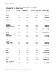
rural population in the Philippines, it was assumed that the proportion
of the population living in rural areas would decrease by the
same ratio (from 65 per cent in 1957 to 56.5 per cent in 1977)as the
decrease in labour force engaged in agriculture and related activities
(from 59per cent in 1957to 51 per cent in 1977). See Population
Growth and Manpower in the Philippines (United Nations publication,
Sales No. 6J.Xm.2), p, 12.
15 See, for example, regression techniques for projecting economically
active population used in various studies described in
Manual V: Methods ofProjecting the Economically Active Population
(United Nations publication, Sales No. E.70,Xm.2), pp, 22-34.
But the regression approach has seldom been used so far to project
urban and rural population.
18 Urbanization: Development Policies and Planning, International
Social Development Review, No. I (United Nations publication,
Sales No. E.68.IV.l), p. 27; Kingsley Davis and Hilda Hertz
Golden, "Urbanization and the development of pre-industrial
areas", Economic Development and Cultural Change (Chicago),
vol. III, No.1, October 1954, pp. 8 and 16; Leo F. Schnore, "The
statistical measurement of urbanization and economic development",
Land Economics (Madison, Wisconsin), August 1961, p, 234.· .
5
It must be noted, however, that even the highest of
these correlations, .87, explains only about three-fourths
of the variance, and .70 would explain only about half
of the variance. Moreover, the variables correlated with
urbanization are often more highly correlated with one
another than with urbanization, 17 so that rather little
additional explained variance should be expected from a
multiple regression approach.
Even though paired projections alone should be used
with caution, they can still serve a useful function by
providing a check on autonomous demographic projections
for what can happen at least demographically may
be constrained by environmental limitations, both economic
and spatial. It would be desirable from the point
of view of economic and social as well as demographic
projections to assemble and analyse the entire correlation
matrix of the many interdependent variables so that the
reactions of the individual variables and combinations
of variables upon each other could be evaluated.
Computerized projections
Economy-based population projections can be calculated
without explicit consideration of probable changes in
demographic trend components, provided that the
assumption can safely be made that the population
required for urban economic growth will be drawn to
urban areas without exhausting its source of supply in
the rural areas. However, changes in fertility and mortality
are likely to modify the ratio of dependants in each
household. Also female labour fource participation may
be affected.18
In projections of urban and rural population for
numerous regions in the Soviet Union, explicit account
was taken of fertility and mortality which were considered
separately for urban and rural areas. The models were
based on a projection technique which has been in use
in the Soviet Union since the first five-year economic
development plan. The volume of migration was
determined by the planning agencies on the basis of
plans for the distribution of productive forces and manpower.
19 In its present detail, the method is very
labour-consuming. For example, to estimate the population
of a particular territorial unit twenty years ahead
under such headings as urban and rural population, male
and female population and so on, taking migration into
account, it is necessary, with 2,000 items of basic data, to
perform over 100,000 calculations. 20 However, with
the use of computers such methods can now be used with
considerable detail, which was not possible previously.
17 Population Bulletin ofthe United Nations, No.7 (United Nations
publication, Sales No. 64'xm.2), pp. 145-147.
18 John Stuart MacDonald, "Anticipating city growth and population
projections for urban development planning", in Proceedings
ofthe World Population Conference 1965, vol. III (United Nations
population, Sales No. 66'xm.7), pp. 72-73.
19 P. G. Podyachikh, "Population projections in which allowance
is made for migration", in Proceedings of the World Population
Conference 1965, vol. III (United Nations publication, Sales
No. 66'xm.7), pp. 83-90; and A. F. Pobedina, "The use of electronic
computers for population projections", in Proceedings of the
World Population Conference 1965, vol. III (United Nations publication,
Sales No. 66'xm.7), pp. 34-39.
20 A. F. Pobedina, op, cit.

Leon Tabah has described a computer model based on
survival ratios which produces simultaneously projections
with cross-classifications of population by sex, age,
economically active and inactive, and urban and rural
areas. 21
Geographic projections
Anticipated area reclassifications can become difficult
to introduce into the calculations ofcertain urban population
projections. At least one detailed attempt has been
made by Jerome P. Pickard, using his own definition of
"urban regions" which are subject to geographic expansion.
The definitions include the rural population
expected to fall within the transportation, communications
and market networks ofthe expanding city-dominated
areas. Pickard projects not only future population of
urban regions, but also the number of square miles that
will be contained within these areas at future dates. A
map area computer was used in this work as well as
census map records and enumeration books for the
United States going back to 1920. 22
Even without detailed geographic information, it is
possible to arrive at approximations of the amount of
land which will come under urban settlement in the
future. The simplest approach would be to project
the future density of total urban population or of a
particular city and to calculate the amount of land that
would be necessary to accommodate the projected urban
population at the projected density. 23 In places where
improvements in transportation are expected, it is often
reasonable to assume a future decrease in density. 24
However, in cases where heavy in-migration is expected
the density may increase. There is also the possibility
that spatial merging of two or more formerly separate
urban areas will alter the average density. There could
even be an agricultural limitation if the urban agglomeration
spreads so far that it becomes difficult for the inner
city population to be supplied with perishable foodstuffs
and consequently the expected returns to agricultural
21 Leon Tabah, "Representations matricielles de perspectives de
population active", Population (paris), May-June 1968,pp, 437-476.
22 Pickard's most extensive study is described in Dimensions of
Metropolitanism, research monograph 14 (Washington, D.C.,
Urban Land Institute, 1967). Other published studies by Pickard
can be found in: "Future growth of major U.S. urban regions",
Urban Land (Washington, D.C.), February 1967; "U.S. urban
regions: Growth and migration patterns", UrbanLand (Washington,
D.C.), May 1966; "Urban regions of the United States", Urban
Land, (Washington, D.C.), April 1962; and Metropolitanization of
the United States, research monograph 2 (Washington, D.C.,
Urban Land Institute, 1959).
23 Such an approach was taken in Department of the Environment,
Long-Term Population Distribution in Great Britain-A Study:
Report by an Interdepartmental Study Group(London, Her Majesty's
Stationary Office, 1971).
24 Kingsley Davis, "Conceptual aspects of urban projections in
developing countries", in United Nations, Proceedingsofthe World
Population Conference 1965 (United Nations publication, Sales
No. 66'xm.7), vol. III, pp, 61-65. Davis found, in a long-run
study of the San Francisco Bay Area, that the population rose
from 364,000in 1890 to 3,217,000in 1960, but the over-all density
declined from 5,643 to 2,501 per square mile, because the territory
expanded at a faster pace than the population. Reference is made
in the article to a book which he published with Eleanor Langlois,
entitled Future Demographic Growth ofthe San Francisco Bay Area
(Berkeleys University of California, 1963).
6
uses of the land exceed the expected returns to urban
uses. On the other hand, where cities grow by merger
with other cities, there may remain pockets of agricultural
land area within the legal city limits. For this reason,
the United States Bureau of the Census has designated
certain cities as "extended cities", and in the 1970 census
figures both an urban and a rural population are shown
for such cities. 25 Since conditions in different places
may vary greatly, no generalized methods can as yet be
proposed. 26
ORGANIZATION OF THIS MANUAL
This manual, being developed by the United Nations
Secretariat, naturally favours those methods of projection
of urban and rural population which it has found most
useful in some of its own work. For its own purposes,
the United Nations requires methods having widest
international applicability, including those countries for
which statistical documentation is only scant. These
methods may be too crude for some countries and too
refined for others since available statistics and actual
conditions vary widely from one country to another.
The user of this manual is encouraged to make his own
adaptations, which, according to judgment, may seem
indicated in the case of his particular country. While,
in these methods, extensive use is made of a logistic-scale
curve (tablulated in annex I), the use can be flexible,
permitting accelerations and slow-downs which might
sometimes be reasonably expected. Reasons for the use
of such a curve are discussed in chapter III. No less
important than the particular schemes of calculation are
problems ofdefinition and formulation of suitable assumptions.
The first three chapters accordingly deal with the
clarification of some basic concepts.
Simple methods for projections of urban and rural
populations (relative to national population totals) are
discussed in chapter IV; the United Nations method is
introduced in chapter V; and its extension to mutually
consistent projections for individual cities is illustrated
in chapter VI. The simple application of the United
Nations method is facilitated by the logistic model
tabulated in annex I.
All these are global methods of type (a), but they need
not be limited to population totals. The consistent
estimation of sex-age composition is always possible,
whether by conventional methods (chapter VII, section A)
or by an extension of the United Nations method (chapter
VII, section B); methods of types (b) and (c) may
26 United States Bureau of the Census, 1970 CensusofPopulation:
Number of Inhabitants: United States Summary (December 1971),
p. ix (preliminary report).
28 Kingsley Davis lists several types of criteria which could be
used in evaluating which area units should be included within the
boundaries of metropolitan areas. See his "Conceptual aspects
of urban projections in developing countries" in Proceedingsofthe
World Population Conference 1965 (United Nations publication,
Sales No. 66'xIII.7), vol. III, pp. 61-65. Even more numerous
criteria have been used on occasion in the efforts of the United States
Bureau of the Census to delineate the contours of metropolitan
areas. See United States Bureau of the Census, United States
Census of Population: 1960 (Washington, D.C., United States
Government Printing Office, 1961), vol. 1, part A, p. xxiv,

nevertheless often be preferable, and these are reviewed
briefly in chapter VIII.
Chapter IX, finally, introduces the more detailed model
of urban and rural population change by demographic
components corresponding to the method of type (d),
which may not be necessary for population forecasts, but
is indispensable for comparative theoretical projections.
A table of survival ratios (P:c) of model life tables for
five-year age groups and five-year intervals of time is
provided in annex II for use in this model.
The manual is designed for a variety of needs. As the
discussions in chapters I through IV are largely prelimi-
7
nary, those readers who need only a simple method for
projecting urban and rural totals which yields at least
reasonably useful results under a wide variety of circumstances
may wish to move directly to chapter V. Chapter
VII explains simple methods for adding sex and age
detail to these projections. Chapter VI tells how individual
cities may be projected. Both chapters IV and VI
are relevant also in the case of a small country most or all
of whose urban population is that of one city. Finally,
those readers who require component methods of varying
complexity may move directly to the last two chapters
of the manual.

j
j
j
j
j
j
j
j
j
j
j
j
j
j
j
j
j
j
j
j
j
j
j
j
j
j
j
j
j
j
j
j
j
j
j
j
j
j
j
j
j
j
j
j
j
j
j
j
j
j
j
j
j
j
j
j
j
j
j
j
j
j
j

Chapter I
PROBLEMS OF DEFINITION OF URBAN POPULATION
1. Before proceeding to a projection, it is necessary to
examine the definitions according to which data on
"urban" and "rural" population have been determined.
Under some definitions, for instance, "urban" areas
remain within constant geographic boundaries, and
"urban" population, so defined, can grow by births,
deaths and migration only. According to some other
definitions, the geographic extent of "urban" areas can
expand continuously; in such a case, the "urban" population
grows by area reclassifications as well as by births,
deaths and migration.
2. Definitions of "urban" localities vary from country
to country, and within the same countries from time to
time. In some countries, moreover, two or more definitions
are maintained side by side. Urbanization being
both a quantitative and qualitative process, different
criteria of "urbanism" gain or lose relevance as time
progresses.
3. A bewildering variety of criteria have been used,
singly or in combination, to define "urban" localities. 27
Essentially, the definitions are mostly of the following
types: administrative, economic and geographic. The
type of definition must be ascertained when a projection
is made since it determines whether or to what extent
"urban" populations can also grow through reclassification
of areas previously defined as "rural". Different
types of definition, moreover, can be suitable according
to the purposes which the forecast is intended to serve.
ADMINISTRATIVE DEFINITION:
TYPE OF LOCAL GOvERNMENT
4. In many countries the minor territorial administrative
units have local governing bodies of diverse forms
or degrees of authority, making obvious the distinction
of those which are of an "urban" type. The administrative
boundaries of urban local governments then
contain the population defined as "urban", all other areas
being classed as "rural". The effects of such a definition
vary, however, depending on the relationship between
administrative area and the area built up at an urban
density, and depending also on the frequency with which
administrative boundary adjustments may occur.
5. The administrative area can be said to be "underbounded"
where there are additional, inmmediately
adjacent, densely built-up areas outside the administra-
27 For a brief survey of definitions of "urban" population in the
censuses of 123 countries taken around 1960, see Growth of the
World's Urban and Rural Population, 1920-2000 (United Nations
publication, Sales No. E.69.xm.3), pp. 7-10.
9
tive boundary, such areas as may be called suburbs,
possibly including administratively separate towns which
have come to form conurbations. The administrative
area can be said to be "over-bounded" when it is more
extensive than the densely built-up area and includes also
some population settled at much lower densities. The
administratively "urban" population can thus be smaller
than the population inhabiting urbanized terrain, and in
some instances it can also be larger. The extent of
coincidence between the two depends largely on administrative
flexibility and on the speed with which built-up
areas have expanded geographically. The administrative
reforms in Japan in 1953, for instance, have had the
effect that most cities, which previously were rather
"under-bounded", suddenly became "over-bounded"
with reference to contiguous built-up areas. As a consequence,
37.5 per cent of the population were classified as
"urban" in the 1950 census, as against 56.3 per cent only
five years later, at the census taken in 1955. While
undoubtedly the urban settlements gained population
rapidly in that period, the apparent growth would not
have been so extraordinary if the administrative areas had
remained the same, or if "urban" population had been
defined on the two occasions in geographic or other
terms. 28
6. Countries vary considerably in the territorial
flexibility of administrative areas. In some countries,
local administrative boundary adjustments are made very
rarely if at all, in others they happen from time to time,
and in still others they occur with great frequency. This
concerns both the recognition of additional areas as
"urban" (through establishment of a new local government
of an "urban" type) and the geographic expansion
of existing "urban" areas through annexation of surrounding
terrain previously under "rural" forms of government.
7. Where administrative boundaries remain unchanged,
the growth of population in densely built-up areas is
not fully reflected by the increases noted in the population
of administratively "urban" areas. This is especially
the case where, with urban growth, there is an increasing
overspill of urbanized settlement beyond the administrative
city limits, as happens generally where the city
28 The 1955 census of Japan included a table showing the 1950
population within areas classified as "urban" in 1955. In all,
53.5 per cent of Japan's 1950 population inhabited the "urban"
areas of 1955. The comparison of figures suggests that between
1950 and 1955 as much as 16 per cent of the population of Japan
were reclassified from rural to urban, and that between 1950 and
1955 the "urban" population ratio rose only slightly. However,
without doubt, effectively urbanized areas within the "urban"
areas of 1955 expanded significantly within the 1950-1955 period,
a circumstance not reflected in this comparison of percentages.

is "under-bounded". In many countries there are now
extensive urban agglomerations whose populations are
multiples of those of the administrative central cities.
In some large cities, because of city-to-suburb migration,
the population of the agglomeration keeps growing even
though the population within the administrative municipal
limits decreases. In the London region population
increases notably in areas situated outside the Green Belt,
whereas in the agglomeration within the Green Belt it
has been decreasing for some time.
8. To a lesserextent this is also true of "over-bounded"
cities within fixed limits. Here, the expansion of the
inner agglomeration is associated with some displacement
or absorption of a population living at hitherto rural
densities. However, since the displaced or absorbed
rural population (with its lotver densities) is usually
comparatively small, the underestimation of rates of
urban growth in most such instances is only slight.
9. The estimation and projection of urban population
trends as defined within unvaried territorial limits has
the advantage that change occurs only as a result of
births, deaths and migration, but not from the reclassification
of previously "rural" areas. Numerous other
statistics referring to such constant areas can often also
be assembled. There is no break of continuity in the
statistical time series. It is convenient in many studies
to compare population and other statistics which are
available for the same fixed area.
10. In a large country where local administrative
boundaries are flexible and frequently adjusted, the trend
in "urban" population (administratively defined) may
closely parallel the trend in the population of physically
urbanized terrain. It can be assumed, in such a country,
that administrative changes are made approximately in
proportion to the geographic expansion of densely
built-up areas. It can also be assumed that territorial
adjustments will be made continuously in the future,
having similar effect. Differences between administered
"urban" terrain and the areas under dense settlement, in
such an instance, may remain unimportant or negligible.
For certain studies, however, the fact that continuous area
changes are also involved must be borne in mind.
11. A problem arises especially in the instance of a
country where administrative adjustments are made
only from time to time. For in this case the adjustments
can be abrupt and discontinuous, and it is difficult to
predict what other modifications of "urban" boundary
willbe made in the future, if any. Projections of administratively
"urban" population can then be scarcely made
except on the uncertain assumption that administrative
limits will remain unchanged. In relation to such an
assumption, the past trend of administratively "urban"
population would also have to be re-estimated in accordance
with the most recent boundaries.
ADMINISTRATIVE DEFINITION:
SEATS OF DISTRICT GOVERNMENT
12. In a number of countries basic administrative
units of one single type cover the entire territory. Each
unit is governed from one city or town situated within it,
10
and the population of these cities or towns is considered
as the "urban" population, the remainder being "rural".
13. In actual fact, the seats of regional (district,
municipality, canton and so on) government are usually
also the centres to which certain particular administrative
measures apply, hence in at least that sense they have a
different type of "local" government. This is typically
the case in Latin American countries. The effects of such
a definition can be similar to those already discussed in
the previous subsection, except under certain limiting
conditions. It can fairly be assumed that, in view of the
degree of regional autonomy, the outer boundaries of the
"urban" centres are usually adjusted to coincide approximately
with those of the built-up urban terrain.
14. Whereas the delimitation of such urban centres may
be flexible, that of the districts (of which they are the
centres) is usually quite rigid. New "urban" centres will
rarely appear because the establishment of new districts
probably occurs rather seldom. This despite the fact
that new compact settlements other than district centres
can also emerge. A new mining town, for instance, may
fail to make its appearance among administrative urban
settlements. Some urban centres, furthermore, may
grow so large that their physical limits encroach on the
territory of neighbouring districts. Unless a territorial
reorganization takes place, part of the growth of large
cities will then fail to be reflected in the population trend
of the "urban" centres of which one is assumed to lie
within each of the districts.
DEFINITION BY SIZE OF ADMINISTRATIVE UNITS
15. In many countries most of the basic administrative
units are quite small, and there is no formal distinction
of those of an "urban" type, all local governments being
similarly constituted (in communes, circumscriptions
and so on). This situation is found especially in some
rather densely populated European countries. Since the
area units are mostly small, the presence of a sizable
population in anyone of them usually indicates the
presence of an urban cluster. Only in exceptional
circumstances would an entirely rural commune comprise
a large population. Moreover, where administrative
areas are generally small, it can often happen that two or
severalneighbouring units are merged into one, permitting
an expanding city to continue being administered as one
unit. Territorially large units may emerge in time
representing in each instance an expanding major city.
Annexation of neighbouring communes into a city
usually occurs only after some time lag, surrounding urban
terrain or "suburbs" still being administered in the interim
as separate units; but these also, for the most part, would
be of greater population size than the more strictly rural
units. The size of individual cities may often not be
sufficiently reflected, but the size of the combined "urban"
population (including separate suburbs which are also
"urban") can well be represented by the population sum
of all those units in which some minimum population size
is exceeded.
16. The minimum size of units to be recognized as
"urban", however, differs greatly between countries,
varying in extreme instances from as little as 100 inhabi-

tants to as much as 30,000. Often the limit is 2,000,
2,500or 5,000. A uniform limit cannot be prescribed for
all countries since typical qualitative features or residential
densities in settlements of a given size may differ
among the countries. A few European countries have
adopted a definition by which units with 10,000 or more
inhabitants are considered as "urban", those with
2,000-9,999 inhabitants as "semi-urban", and those with
less than 2,000 as "rural".
17. The trend of "urban" population defined in this
fashion may well parallel that of population in built-up,
urbanized areas. Part of the "urban" population growth
will result from the surpassing of the minimum "urban"
population size by additional administrative units, as a
result of which those units are reclassified. But the
growth of individual big cities may be inadequately
reflected so long as many suburbs continue being administered
separately.
ECONOMIC DEFINITION, APPLIED TO
ADMINISTRATIVE UNITS
18. In some countries, where basic administrative units
are small and uniform, "urban" administrative units are
definedas those in which at the most a smaIlpercentageless
than some stated maximum-of the economically
active population (or active males) are engaged in agriculture.
There are also some countries where units are
defined as "urban" by combined criteria of size and type
of economic activity.
19. Such a definition is of value particularly in those
countries where some agricultural villages are apt to
grow larger than some small towns in which urban
features predominate (e.g. mining towns, small suburbs,
local trading centres). In such countries, evidently, a
definition based on an economic criterion has greater
relevance than one based on population size only.
Though it is recognized that non-agricultural activities
exist in areas settled in a rural fashion, and that there can
also be a small amount of agriculture among urban
residents, the coincidence of a prevalence of agriculture
with other features describing a rural environment
usually remains considerable.
20. The effectof such a definition on population trends
in "urban" places is similar to that where the definition
merely involves a size limit. Administrative units are
added to the "urban" category, in this case, when nonagricultural
activities in them come to outnumber the
agricultural ones to the extent implicit in the definition.
It is difficult, however, to assess the past and future trend
for "urban" areas so defined. Where it is a matter of
size limit only, the population estimates themselves
express whether an "urban" size has been or probably
will be attained at given dates. It is not so easy to
estimate and project trends in the agricultural and nonagricultural
composition of the labour force in each
individual locality.
GEOGRAPHIC DEFINITION: AGGLOMERATIONS
21. The internationally recommended definition of
"localities" is that of population clusters within the
11
contours of dense settlement, irrespective of administrative
deliminations. This concerns localities of every
size and economic type. The "locality" may consist of
a small grouping of rural houses (e.g. a hamlet as distinct
from completely dispersed rural population) and, at the
other extreme, of an urbanized region comprising several
administrative cities, assuming that the urbanized areas
have coalesced. Among localities so delimited one may
select those above a certain size, or those having mostly
non-agricultural activities, to define "urban" agglomerations.
It is evident that agglomerations expand geographically
whenever there is building activity at their
periphery. Upon occasion, two or several neighbouring
agglomerations merge into one.
22. In some countries the delimination of agglomerations
on the occasion of a census is made on the basis
of detailed map work including, as in Sweden, the measurement
of distance between individual houses to determine
which of them should be considered as included in
the same agglomeration. But simpler determinations
can be made, for instance, by using as units the groups
of contiguous census enumeration districts in which a
minimal population density is exceeded. The boundaries
of the agglomerations may then not be determined with
geographic precision but nevertheless accurately enough
for demographic studies. In the United States, "urbanized
areas" are established at each census, adjacent to
administrative cities of at least 50,000 inhabitants. In
Japan, any group of contiguous census enumeration
districts having more than a certain high population
density and a combined population of at least 5,000
inhabitants are referred to as "densely inhabited districts".
It is possible of course that both in Japan and in the
United States densely urbanized areas smaller than entire
census districts are not included, hence that the urbanized
area is somewhat under-bounded. Other methods for
an approximate delimitation of agglomerations have
come into use elsewhere, such as the multicommunal
agglomerations which have been defined in France.
23. Speaking somewhat schematically, one may say
that a major agglomeration, or "urbanized area", ordinarily
consists of a central city (i.e. an administrative
urban unit) together with densely urbanized "tentacles"
branching out alongside the major routes of travel,
whether roads, rails or waterways. Such an urban
"octopus" may with time absorb within it other urban
centres, e.g. satellite towns, or it may come in contact
with one or several neighbouring "octopuses" thus
forming a conurbation. Between the extended "tentacles"
there remain areas inhabited at lower densities
which must still be regarded as rural. Geographic
growth of the "octopus" occurs through a lengthening and
thickening of the "tentacles" and lateral outgrowths,
from them which, with time, form a tissue of lateral
connexions. Actually, of course, particular geographic
features, if not also deliberate action, for instance the
construction of a circular road around the city, will
prevent agglomerations from attaining precisely such a
schematic shape.
24. The noteworthy fact remains that the growth of
agglomerations is an accurate reflection of the areas
inhabited under physical urban conditions, i.e. at urban

densities. The trends of growth include the transformation
of previously "rural" into "urban" areas, hence they
imply area reclassifications.
25. The analysis and projection of urban populations
in terms of all agglomerations above some minimum
size has certain drawbacks, however. On the occasion
of each population census the areas have to be delimited
afresh. It is not possible to follow their continuous
expansion through intercensal or postcensal time periods.
Nor is it possible, for areas whose limits differ from any
administrative boundaries, and which vary continuously,
to organize the collection of other statistics, such as
those on births, deaths, school enrolment, retail trade,
motor vehiclelicenses, and so forth.
26. Since usually only major cities and towns are
demarcated in a census as agglomerations, small towns,
though they may have markedly urban features, remain
omitted from this special "urban" category, unless they
are already absorbed in a major agglomeration. The
combined population of the selected major urbanized
areas is generally less than the country's combined
"urban" population under a definition which can include
far more numerous smaller cities and towns.
GEOGRAPHIC DEFINITION: METROPOLITAN AREAS
27. As has already been noted, administrative definitions
often remain confined to constant areas, reflecting
only part of the urban growth, with consequent insufficiencies
in the measurement of the urban phenomenon.
The definition of geographic agglomerations reflects the
expansion of urban environments quite realistically, but
has the disadvantage that no statistics other than those
determined at each censuses can be collected for them,
since their contours change continuously. Mainly to
circumvent the disadvantages inherent in both types of
definition, another concept has been formulated, namely
that of metropolitan areas.
28. The metropolitan areas are usually conceived in
such wide limits that they include all, or virtually all,
of each agglomeration "octopus" and, in addition, the
non-urbanized areas lying in the interstices between its
"tentacles". The boundaries are drawn in such a way
that they coincide with the outer limits of a group of
existing minor administrative areas which are unlikely
to change. These boundaries can, for a period of time,
be left unaltered, and various types of statistics for each
such group of administrative units can also be continuously
secured. Reclassification of areas from "nonmetropolitan"
to "metropolitan", under these conditions,
need not occur for some time. Of course, the average
population density of metropolitan areas within their
wide limits, is much lower than that of the more strictly
urbanized terrain.
29. The determination of administrative units to be
included in a metropolitan area often involves some quite
precise criteria, such as the frequencies in travel and
communications to and from the central city, establishing
a high degree of economic and social interdependence
with the city. Some areas under rural forms of settle-
12
ment are included where proximity to the city presumably
exerts a major influence on their types or methods of
land use; hence it is not illogical to include them within
the wider urban periphery. In a few instances, groups
of contiguous metropolitan areas have been described as
a "megalopolis".
30. Again, the determination of metropolitan areas
is usually confined to major cities only (e.g. those whose
centres have at least 50,000 or 100,000 inhabitants),
leaving numerous separate towns which form no part of
the metropolitan areas. On the other hand, partly
because of actual internal economic interdependence and
partly because of statistical convenience, metropolitan
areas have often become official planning regions in
programmes of regional development.
31. When compared with the corresponding agglomerations,
the metropolitan areas can be considered as
"over-bounded" urban entities. As has already been
noted, in "over-bounded" cities rates of city growth
are more adequately reflected than in "under-bounded"
ones, owing to the comparative smallness of the rural
population which becomes displaced or absorbed as a
result of the urban expansion. The extensivedelimitation
makes it possible in many countries, where urban growth
is not too rapid, to maintain a constant demarcation of
metropolitan areas over extended periods of time.
Eventually, however, a redefinition of metropolitan
areas can become necessary because of continued geographic
expansion of the corresponding agglomerations
and a further widening of their spheres of influence.
Where this happens, "geographic" methods of population
projection may have to be adopted.
32. Because of the emerging new settlement patterns
around the cities of industrialized countries, it will
probably become increasingly useful to distinguish four
types of areas, namely urbanized and non-urbanized areas
within metropolitan regions, and urbanized and nonurbanized
areas outside such regions. So far, few
censuses permit the distinction of areas according to
such a four-fold classification.
OTHER DEFINITIONS
33. In some countries urban areas have been defined
as administrative units presenting certain "urban features".
Among such features there might be the network of paved
streets, numbered houses, streetlights, domestic electricity,
sewerage, mail delivery, the presence of a secondary
school, a church, a medical establishment, a police station
and so forth. The use of qualitative data describing
urbanism has much conceptual appeal since, according
to the conditions in a country, those might indeed appear
to be the most distinguishing features. On the other
hand, in the context of trend study and projection, the
"urban" significance of any such features cannot be
considered as permanent. Whereas at one time electric
light or police stations may be mostly confined to urban
areas, eventually such features can also spread over the
countryside. The significance of an "urban" definition
expressed in terms of such descriptive attributes can
change with the passing of time.

Chapter n
COMPONENTS OF URBAN AND RURAL POPULATION CHANGE
38. Even though it may be preferable to use only
crude methods in forecasts of urban and rural population,
some knowledge of the underlying dynamics will help
in exercising good judgement. It is perhaps best to
begin a discussion of components of population growth
with a consideration of sex-agestructures. The composition
of populations by sex and age is a consequence of
preceding population trends (births, deaths and migration).
In its turn, this structure partly determines
current and future demographic trends because each of
the trend components, births, deaths or migration, have
a varied incidence among population groups distinguished
by sex and age. Reclassification is an additional factor
which can affect the population composition.
DIFFERENCES BETWEEN URBAN AND
RURAL SEX-AGE STRUCTURES
39. The United Nations Secretariat has made a
survey of sex-age patterns in urban populations throughout
the world. It was found that each national population
is urbanized to a varied extent when every sex-age
group is considered separately. It was found, furthermore,
that the sex-age patterns of urbanization vary
among different parts of the world, no doubt owing to
a diversity of social, economic and cultural conditions
underlying urbanization trends, in factors causing
differences between urban and rural fertility and mortality,
and in the selection of rural migrants proceeding
to urban areas by sex and age. 29
40. Estimates have been made for 1960, largely based
on census data, of the sex-age compositions of the urban
and rural populations in eight major areas of the world,
as summarized in table 1. It will be noted that in all
eight areas the percentages of children, up to the age of
15, are smaller in urban as compared with rural places,
certainly as a result of lower urban than rural birth
rates. Likewise, in all areas the urban population has
larger proportions at ages 15-44 than does the rural
population because urban places attract especially those
persons of principal working ages. In Europe, Northern
America, Latin America and Oceania, but not in the
other major areas, middle-aged and elderly adults are
also relatively more numerous in urban than in rural
places. It is probable that at least in these regions
29 See "Sex and age patterns of the urban population" (ESA/
P/WP.36); "Comparative regional typology of urbanization patterns
by sex and age" (ESA/P/WP.42); and "Sex-age composition of the
urban and rural population of the world, major areas, regions and
individual countries in 1960" (ESA/P/WP.44).
14
rural migrants, once settled in urban localities, prefer
to remain there also at advanced ages.
41. The ratio of males to females, of all ages, is much
greater in urban than in rural areas in South Asia and
Africa, while the reverse is true in Northern America,
Latin America and Oceania, and to a lesser extent also
in Europe. Below age 15, except those aged 5 to 14 in
Latin America, urban and rural sex ratios are nearly
the same as might be expected since a majority of children
of either sex will ordinarily reside with their parents. The
high rural sex ratio in Northern America at ages 15 to
24 may in part be attributed to the stationing of military
troops in rural localities. But probably for different
reasons the excess of males over females aged 15 to 24
in rural areas is also considerable in Latin America and
Oceania. In South Asia and Africa, by contrast, there
is a considerable excess of males in urban areas at ages
15 to 24, and an even greater excess at ages 25 to 44.
But despite such regional diversity, and for unknown
reasons, at ages 65 and over all major areas show a lower
urban than rural sex ratio, and the difference between the
two is greatest in Northern America, Latin America and
Oceania.
42. The economic, social and cultural reasons for such
a diversity in regional modes of urbanization have not
yet been systematically studied, 30 but it is evident that
the age structures reflect urban-rural differences in demographic
trends (fertility, mortality and migration). Since
urban and rural structures differ so much, it is of considerable
interest to detail urban and rural population projections
according to sex and age. In the choice of a suitable
method to obtain such results, it is of some importance to
appreciate the relative roles of the several demographic
trend components in producing such effects.
URBAN RESIDENCE RATIOS BY SEX AND AGE
43. There is a more direct way to analyse the structural
differences between the urban and rural population. If
we can assume a sufficient degree of population mobility
between the two types of residence (urban, rural) we can
consider the percentage urbanized, in each sex-age group,
as reflecting a specific preference for residence in urban,
rather than rural, areas, varying according to sex and
age. Those sex- and age-specific "urban residence
ratios" can therefore be plotted in a curve much as one
30 One further United Nations study suggests that there is an interrelation
between patterns of urbanization and patterns of marital
status, both of which may be partly determined by the role and
status of women in a society. See "Urban-rural differences in the
marital status composition of the population" (ESA/P/WP.5l).

- All VI
TABLE 1. PERCENTAGE AGE COMPOSITION OF MALE AND FEMALE POPULATIONS, AND AGE-SPECIFIC SEX RATIOS,
IN URBAN AND RURAL AREAS IN EACH OF EIGHT MAJOR AREAS OF THE WORLD, AS ESTIMATED FOR 1960
East Asia South Asia Europe Soviet Union Africa Northern America Latin America Oceania
------
Group Urban Rural Urban Rural Urban Rural Urban Rural Urban Rural Urban Rural Urban Rural Urban Rural
Males
All ages ....................... 100.0 100.0 100.0 100.0 100.0 100.0 100.0 100.0 100.0 100.0 100.0 100.0 100.0 100.0 100.0 100.0
()-4 ......................... 12.8 15.2 14.7 17.1 8.8 10.3 11.5 14.4 15.6 18.1 11.8 17.4 15.6 18.1 10.8 14.9
5-14 ............. . . . . . . . . . . . . 21.0 25.2 23.8 25.4 16.6 19.5 19.7 23.6 22.6 26.5 19.8 21.8 23.8 27.5 19.7 23.3
15-24 22.1 18.1 21.3 18.2 15.6 15.1 19.2 16.9 21.6 18.6 13.2 15.6 18.1 18.3 14.3 16.6
•••• 0 •• ••••••••••••••••••
•••••••••••••••••••• 0 •••• 25-44 28.8 24.7 26.9 24.6 27.8 25.4 31.0 24.8 28.3 23.0 27.2 23.6 25.8 22.1 27.8 25.8
•••••••••• 0 •••••••••••••• 45-64 12.7 13.1 11.1 11.6 23.3 21.4 15.1 14.4 10.0 10.9 20.1 18.6 13.0 11.0 20.0 14.8
65 and over ................... . 2.6 3.8 2.3 3.1 8.0 8.3 3.5 6.0 2.0 2.8 7.9 9.1 3.7 3.0 7.4 4.6
Females
•••••••••••••••••• 0 •••• ages 100.0
()-4 ........................ . 12.9
100.0
14.7
100.0
15.9
100.0
17.3
100.0
7.6
100.0
9.5
100.0
9.1
100.0
11.2
100.0
16.8
100.0
17.5
100.0
10.8
100.0
11.8
100.0
14.4
100.0
18.6
100.0
10.1
100.0
15.9
5-14 .........................
15-24 .........................
25-44 .........................
•••••••••• 0 •••••••••••• • • 45-64
65 and over ........ ·· .... ·· .. ··
21.1
21.2
28.3
13.0
3.7
24.3
17.8
24.8
13.8
4.6
25.5
20.2
24.7
10.8
2.9
25.6
17.7
24.6
11.7
3.0
14.5
14.1
27.2
25.0
11.6
18.2
13.9
25.2
22.5
10.1
15.9
16.5
31.1
20.4
7.0
18.6
13.2
25.6
21.6
9.8
25.4
20.9
23.9
10.3
2.8
25.6
18.5
23.7
11.4
3.2
18.2
13.4
27.2
20.6
9.8
22.3
13.6
24.2
18.4
9.7
23.0
18.6
26.1
13.5
4.4
27.8
17.9
22.2
10.5
3.0
18.7
14.1
26.4
20.3
10.3
24.6
16.0
25.1
13.8
4.6
Males per 100females
All ages •• 0 •••• ••••••••••••••• •
0-4 .........................
5-14 .........................
15-24 .........................
25-44 .........................
45-64 .........................
65 and over ....................
103
103
103
108
105
101
74
99
102
103
100
99
94
82
112
104
105
118
122
115
89
102
104
104
97
102
105
97
91
105
104
100
93
85
63
97
105
105
106
98
93
76
83
105
103
97
83
62
42
82
105
98
105
79
55
51
110
102
98
114
130
107
80
97
100
100
98
93
93
84
94
104
103
93
95
92
76
108
104
105
123
105
108
101
95
103
98
92
94
91
80
106
104
105
109
106
112
105
99
105
104
100
104
97
71
113
106
108
117
116
121
112

can plot age-specific labour force participation rates,
or age-specific percentages of married population,
entries and departures from the category being possible
at each age so as to result in a curve. There is, however,
an important exception in the factors causing the varied
urban residence ratios: the children of either urban or
rural parents have no free choice of residence and ordinarily
stay with their parents, or at least with theirmothers.
Only as age progresses into adolescence and beyond can
one note the effects of the varying balance between
entries into and departures from urban residence.
44. Almost invariably the urban residence ratios
attain a peak near those ages at which migration is most
frequent. 31 The age of greatest peak comes a few years
of age sooner for females than for males. The height of
the peak, on the whole, is greater for men than for women
in Africa and Asia, but it is greater for women than for
men in Latin America and in most of the more developed
countries. Countries differ in the shape of the curve
at ages past the peak. In some countries, for instance,
a second peak appears at some more advanced ages,
after an intervening depression. Probably the shape of
the curve reflects to a considerable extent the past trends
of net rural-to-urban migration which, of course, could
have fluctuated. To an undetermined extent, however,
the curve is also influenced by comparative levels and
trends in urban and rural fertility, and mortality, respectively.
As is known, age structure can be greatly affected
by varying fertility trends of the more or less distant past,
but only to a minor extent by varying mortality trends.
TABLE 2. PERCENTAGE OF NATIONAL SEX-AGE GROUPS RESIDING
IN URBAN AREAS, CoLOMBIA 1964 AND IRAN 1966
Colombia 1964
Iran 1966
Age (years) Males Females Males Females
0-4 .............. 49.1 49.5 35.0 35.6
5-9 .............. 48.5 49.8 35.9 36.3
10-14.............. 49.3 53.7 42.0 42.6
15-19.............. 50.7 60.3 46.9 42.9
20-24.............. 51.4 58.5 51.2 42.2
25-29.............. 51.8 57.0 41.5 38.2
30-34.............. 52.4 57.0 38.7 37.5
35-39.............. 49.3 55.1 38.7 40.6
40-44.............. 49.1 55.1 36.8 36.6
45-49.............. 47.8 55.6 39.8 42.2
50-54.............. 47.3 56.2 39.8 41.8
55-59.............. 49.0 58.3 37.1 41.3
60-64.............. 45.3 56.7 37.7 38.7
65-69.............. 49.0 59.1} 35.4 36.5
70 and over ........ 46.2 57.2
Almost invariably, the urban residence ratios for small
children fall below the level for women of ages at which
they might be their mothers; this is a reflection of a
usually lower fertility in urban areas as compared with
rural ones. To illustrate this rather summary statement,
the relevant ratios for Colombia (1964) and Iran (1966)
are shown in table 2 and figure 1.
31 As further examined from intercensal balances in "The dynamics
of rural-to-urban population transfers by sex and age" (ESA/P/
WP.48).
16
45. An exact interpretation of the graphs is not possible
owing to the accumulation of various effects in the course
of time. Nor are the data very accurate: zig-zags at
advanced ages can be the result of a different incidence of
age misstatements in urban as compared with rural areas.
A few facts are evident nevertheless: the young migrants
to urban areas are predominantly female in Colombia
and predominantly male in Iran: in both countries, female
migrants are somewhat younger, on an average, than
male migrants; in both countries, as witnessed by childwoman
ratios, urban fertility is lower than rural fertility;
and whereas probably most female migrants in Colombia
establish permanent residence in urban areas, in Iran the
residence of many young male migrants in urban areas
is probably more temporary, leaving smaller balances
past the age of 25. The impressions may be partly
falsified by inaccuracy in the age data, and by possible
and unknown fluctuations in net migration during
decades of the past.
DIFFERENCES BETWEEN URBAN AND
RURAL CRUDE DEATH RATES 32
46. Conditions affecting mortality are apt to differ
between urban and rural areas. For instance, in urban
places medical facilities are more readily accessible. On
the other hand, risks of contagion or motor vehicle
accidents are probably less in the rural areas. Because
of a differing incidence of various forms of pathology,
it is possible that one of the two environments has relative
advantages for persons of one or the other sex, or for
individuals of different age. Whether, on balance,
mortality is heavier in cities or in the countryside is a
little-researched subject. It is believed that, because of
the relative lack of health services, rural mortality appreciably
exceeds the urban in the less developed countries,
but it is not known how large the difference may be in
the typical instances. In the more developed countries
medical and sanitary services are very widely available,
and mortality is generally so low that the differences
between urban and rural areas cannot be very wide.
47. The United Nations has carried out some calculations
of what the urban and rural crude death rates could
have been around 1960 if mortality conditions in each
region had been the same in urban and rural areas. Then
assuming some differences at least in the less developed
regions, the United Nations also calculated what the
crude death rates might actually have been under those
assumptions.P with further adjustments in these rates
to make them compatible with a basic set of United
Nations estimates pertaining to regional rates of population
growth. The two sets of results are shown in table 3.
32 In this and the following two sections, estimates are discussed
as calculated in "The components of urban and rural population
change: tentative estimates for the world and twenty-four regions
for 1960" (ESA/P/WP.46).
33 It was assumed that urban expectation of life at birth exceeded
the rural by 5 years in East Asia (except Japan), South Asia, Africa,
Melanesia, Polynesia and Micronesia, and by 2.5 years in Latin
America. In Japan, Europe, the Soviet Union, Northern America
and Australia and New Zealand urban and rural mortality were
assumed to be the same.

TABLE 4. URBAN AND RURAL CRUDE BIRTH RATES WHICH WOULD RESULT IF URBAN AND
RURAL FERTILITY WERE THE SAME, AND AS ACTUALLY ESTIMATED, AROUND 1960
Assuming equal urban and
rural fertility in each As actually estimated
major area (with adjustment)
Urban Rural Urban Urban Rural Urban
birth birth minus birth birth minus
Major area rate rate rural rate rate rural
East Asia ...................... 40.0 35.2 4.8 29.9 36.8 -6.9
South Asia ••• 0 •••••• • •••••••••
Europe ........................
44.6
19.5
44.5
17.9
0.1
1.6
40.1
17.8
47.4
21.8
-7.3
-4.0
Soviet Union .................... 27.2 22.4 4.8 20.9 26.6 -5.7
Africa ..........................
Northern America ..............
47.3
25.4
47.4
22.1
-0.1
3.3
41.8
24.3
48.0
24.9
-6.2
-0.6
Latin America .0 •••••••••••••••• 43.7 37.0 6.7 35.3 44.5 -9.2
Oceania ••••••••••• 0 •••••••••••• 28.1 26.5 1.6 22.4 36.6 -14.2
Africa, about 6 points less in East Asia and South Asia,
and considerably less also in Oceania; in Europe and
Northern America, on the other hand, the difference, if
any, could have been only slight.
DIFFERENCES BETWEEN URBAN AND
RURAL CRUDE BIRTH RATES
49. Virtually throughout the world the fertility of
urban women is lower than that of rural women, and in
many instances the difference is large. Fertility decline,
where it has occurred, usually began first in urban areas
and spread to rural areas later on. Thus, the urbanrural
fertility difference can widen for a time, to narrow
down again when the general declinein fertilitycomesto an
end. The reasons for such differences between urban and
rural fertility appear to be manifold. Various factors
usually associated with loweredfertility, such as education,
public health, non-agricultural activities, the economic
activity of women, the prevalence of salaried employments
and so forth, are associated with urbanization;
hence it cannot be said to what extent the urban habitat
itself, as an isolated factor, contributes to this fertility
difference. One factor, which has not been sufficiently
explored may be the differentincidence of marriage among
young urban or rural women: sinceurban women generally
marry at a later age or more often remain single, the
general fertility of urban women can be expected to be
lower than that of the rural for this reason alone. 34
50. Without going into the discussion of possible
causes, we refer to United Nations estimates of urban
and rural crude birth rates around 1960,analogous to the
estimates of death rates already discussed. Comparison
is made of the figures shown in table 4.
51. If fertility, calculated as the average number of
births to women aged 15 to 44 years, were the same in
urban and rural areas, differences between urban and rural
crude birth rates would result as shown in the first three
columns of table 4. These differences would have been
due entirely to differences between urban and rural
84 In fact, women's age at marriage is almost everywhere higher
in urban as compared with rural areas; and the proportions of
married women are markedly lower in urban as compared with
rural areas: "Urban-rural differences in the marital status composition
of the population" (ESAjPjWP.51).
18
sex-age compositions. On this hypothetical basis, the
urban birth rates would generally exceed the rural birth
rates because of the prevalence of young adults in the
urban areas. However, as already noted, in some
regions the urban population has comparatively few
women, and mainly for this reason equal urban and rural
fertility would produce only a negligible difference
between the hypothetical urban and rural birth rates of
South Asia and Africa. In Latin America, where women
predominate in the urban population, equal fertility
would cause the urban birth rate to exceed the rural by
nearly 7 points. Considerable excesses of the urban over
the rural crude birth rate would have occurred also in
East Asia, the Soviet Union and Northern America.
52. Actually, however, as calculated by reverse-survival
of sex-age data, the urban crude birth rate was in general
considerably below the rural crude birth rate. Only in
Northern America was the difference rather slight. In
Europe, the rural birth rate exceededthe urban by 4 points,
in the Soviet Union and Africa by about 6 points, in
East Asia and South Asia by about 7 points, in Latin
America by 9 points, and in Oceania by 14 points. 35
DIFFERENCES BETWEEN URBAN AND
RURAL RATES OF NATURAL INCREASE
53. On the basis of age composition only, as has been
argued, the urban areas would have higher crude birth
rates and lower crude death rates than the rural areas.
Therefore, on this hypothetical basis, the urban areas
would have a greater potential for natural increase,
assuming that urban and rural fertility and mortality
could be equal. In actual fact, however, both the birth
rates and the death rates are lower in urban than in rural
places, and often the excess of the rural over the urban
birth rate is greater than the excess of the rural over the
urban death rate, with the consequence that the rate of
natural increase is generally somewhat lower in urban,
as compared with rural, populations. This reasoning
is illustrated in table 5, showing the rates of natural
increase which result from subtraction of the death rates
36 In the case of Oceania it should be noted that most of the
urban population is that of Australia and New Zealand, whereas
much of the rural population is that of Melanesia, Polynesia and
Micronesia.

up to an advanced age. But where migration leads
largely to continued urban residence, migrants of earlier
date remain in the urban population at all ages following
the age of peak migration. If a survey were to be made,
it would be difficult to distinguish between the "floating"
migrants and the more permanent migrants; persons
who have migrated to town will often not know themselves
whether they are likely to leave soon, or whether they are
apt to stay a longer time or even indefinitely. In those
few countries where the census draws a distinction between
de jure and de facto population, the differences
between the two categories in urban areas reflect to some
extent the presence of temporary migrants.
58. The type of migration to urban places will also
depend in part on the census definition of "urban" areas,
already discussed. For instance, in many countries
there is a considerable migration from city centres
toward the suburbs. Often this is a migration of mature
adults, perhaps aged in their thirties, who, having made
a successful beginning in an economic career, wish to
settle their young families in the more favourable suburban
housing conditions. Where suburbs do not
form part of the definition of "urban" localities, the
so-called "urban" places may gain young adult migrants
(aged, say, in their twenties), while losing those aged in
their thirties together with their young children.
59. A desirable type of census data for population
projections (usually carried out in five-year time intervals)
would be those on places of residence five years
previous to a census in relation to their places of current
residence. Five-yearly migration rates, immigration as
well as emigration, would then be directly calculable.
The data would be even more fruitful if it could be
determined whether the previous place of residence
(such as, five years ago) was urban or rural.P? but such
figures are seldom secured as well as difficult to obtain
because ofpossible definitional changes in urban and rural
localities. A question remains also whether the places
of previous residence have been stated accurately in the
census.
EFFECTS OF RURAL-TD-URBAN AREA
RECLASSIFICATION
60. Depending on the kind of definition involved,
rural-to-urban reclassifications can occur especially in
two types of areas: (a) in villages or other settlements
attaining the status of "towns"; and (b) in suburban
areas being annexed by the administrative authorities of
geographically expanding cities. The consequence in
either event is a transfer of population from the rural
to the urban category. Census data describing the
sex-age composition of the transferred population are
rarely available. The study of data in those countries
where they are provided gives some indication of possible
effects of these transfers upon the sex-age composition
of the rural and the urban population.
61. If it is only a matter of rural localities attaining
urban status, it can be conjectured, very roughly, that
the sex-age composition of the marginal population
87 Such data have been found in censuses of India and Greece.
See Manual VI: Methods of Measuring Internal Migration (United
Nations publication, Sales No. E.70'xm.3), p. 37.
20
involved is of a type intermediate between the typical
compositions of urban and rural populations, respectively.
This can be approximately the case because the
localities concerned may usually have characteristics
which place them near the border line between the two
types of settlement. In a country whose population is
about 50 per cent urbanized, it is possible that the sexage
composition of the reclassified areas resembles that
of the combined national population. In less urbanized
or more highly urbanized countries this should generally
not be expected.
62. An example of sex-age compositions of populations
in localities ofdiffering size groups is provided in a special
report of the 1965 population census of Japan. Table 6
shows percentage compositions of Japan's total population
and of its population in different community size
groups. 38 In examining these data it should be borne in
mind that Japan is now a highly urbanized country. Two
significant observations can be made. First, the percentage
compositions vary in almost continuous fashion, as
we proceed from settlements of the largest to those of
the smallest size. For instance, males aged 20 to 24 years
constituted 7.3 per cent in cities of 500,000 or more
inhabitants, while in successively smaller localities they
constituted 4.9, 4.2, 3.4, 3.0, 2.6 and 2.4 per cent. Secondly,
the national sex-age composition ofthe population is
most nearly approximated in towns having around 50,000
inhabitants. As a matter of fact, in 1965 nearly halfthe
population ofJapan inhabited towns ofthis size and larger.
63. If it is a case of annexation of suburban areas,
the matter may be quite different. Aside from migratory
balances between the urbanized areas and the rest of the
country, important balances also usually exist between
the central parts of each city and its suburbs. The latter
migration is usually highly selective of groups of sex and
age. In the United States, for instance, the suburban
areas tend to be settled by men of career ages and their
respective families, hence the suburbs have higher
percentages of small children and persons in their thirties
than do the city centres, whereas the latter have higher
percentages of adolescents and young adults, as well as
of adults in mature and advanced ages.
64. Census data for 1960 have been provided for major
cities in the United States whose territory had been
enlarged as a result of annexations between 1950 and
1960. 39 Percentages in each sex-age group of the
combined city population residing in annexed areas can
be calculated, and table 7 presents the results for the
city of Dallas. The same data are also charted in
figure II. As can be seen, the above statement regarding
suburban population is well borne out. It is rather
probable, however, that in a city like Dallas much of
the migration to the annexed areas occurred subsequently
88 Japan, Bureau of Statistics, 1965 Population Census of Japan:
Results by Population Size of Shi, Machi and Mura and of DID's
(Office of the Prime Minister). The calculation was made for shi,
machi and mura, those being the minor administrative divisions of
the country.
38 Miller and Varon, Population in 1960 of Areas Annexed to
Large Cities of the United States between 1950 and 1960 by Age,
Sex and Color, Analytical and Technical Reports No. 1 (Philadelphia,
University of Pennsylvania, Population Studies Center,
November 1961).

were less, namely 21 per 1,000 in South Asia, 18 per
1,000 in Africa, 13 per 1,000 in Latin America and
Oceania, and 9 per 1,000 in East Asia; in Europe, the
Soviet Union and Northern America, the rural population
underwent slow decreases. Relative to the size of the
rural population, outgoing population transfers occurred
at rates of 16to 20 per 1,000in Europe, the Soviet Union,
Northern America and Latin America, at 10 per 1,000 in
Oceania, at 9 per 1,000 in East Asia, and at comparatively
low rates in South Asia and Africa whose rural populations,
relative to the size of the urban, were still very
large. 42 The proportion ofrural natural increase disposed
of by transfers to urban areas was thus 137 per cent in
Europe, 112 per cent each in the Soviet Union and
Northern America, 60 per cent in Latin America, 51 per
cent in East Asia, 43 per cent in Oceania, 21 per cent in
Africa, and 12 per cent in South Asia.
IMPLICATIONS FOR PROJECTION METHODOLOGY
69. The foregoing review of components of urban and
rural population change and of their influenceupon urban
and rural population structures demonstrates a complexity
of factors difficult to isolate from each other unless the
available statistics reflect all that detail with great accuracy.
70. To recapitulate, the urban and the rural populations
can change by the incidence of urban and rural
mortality, urban and rural fertility, internal migration
from rural to urban and from urban to rural areas,
international migration from abroad to urban and rural
areas, and the population of previously rural localities
being reclassified to an urban status. The incidence of
all these events varies to an important degree by groups
of sex and age, and it will be recalled that age itself
changes as time progresses.
71. If we consider the urban population only we can
derive a schemeof its change as follows. Let U; and Ui be
the urban population at the beginning and at the end of a
time interval t; B the number of births occurring during
that interval; D the number of deaths; Ii internal migrants
from rural to urban areas; Ie internal migrants from urban
to rural areas; Ei migrants to urban areas from abroad;
Ee urban emigrants to other countries; and R the population
being reclassified; we arrive at the equation
Ui = Uo + B - D+ li - Ie + Ei - Ee + R
72. If the time interval t is very short, only a few
individuals will undergo more than one of the indicated
events. Over a longer period of time, such as in the
course of five years, many individuals may experience
two or several of the events noted in the equation.
Thus, one person may move from the rural to the urban
area, then emigrate abroad and then return to a rural
place which in turn undergoes urban reclassification still
within the same time period. In the first event, he is
added to the urban population; in the second event, he is
42 As it happens (see also the first section of this chapter), the
highest rates of rural out-migration occurred mainly in those
regions where women predominated among the migrants; where the
migration consisted mostly of men, the rates of rural out-migration
were lower.
23
subtracted; in the third event, he is not registered in the
urban population at all; and in the fourth event, he is
again added. The net result is the addition of one
individual to the urban population, but the events have
been several. The fictitious example illustrates that the
several events depend not only on the initial urban population,
but on an urban population which changes while
these and other events, some of them partly interdependent,
occur. A complete independence of different
events from each other can be postulated only when the
time interval is infinitesimally short.
73. Some degree of statistical stability-whether a
constant level, a continuous trend or fluctuations-can be
imputed to the flow of events when these are taken in
proportion to the population at risk of experiencing
these events. Annual events occurring per thousand of
the population at risk constitute demographic rates. 43
However, some difficulties occur in determining which is
the population "at risk".
74. Clearly it is the urban population itself that is at
risk of experiencing urban births and urban deaths.
On the other hand, it is the rural population (and also the
population of other countries) which is at risk of sending
migrants to the urban areas. Furthermore, the rural
population, or at least some sections of it are at risk of
being reclassified to an urban status. 44
75. In this connexion, it must be pointed out that
the population "at risk" of sending emigrants from the
urban areas is not necessarily the urban population itself.
Many of the persons leaving an urban area are previous
immigrants, either from a rural area or from abroad, who
after a period of urban residence return to their places of
origin. In so far as this is the case, the migrant population
is the one "at risk". And since the risk of generating
this migrant population (at least the internal migrants)
pertains to the rural population of origin, it might even
be said that the rural population itself is at risk of receiving
back some of its previous emigrants. 46
76. Statistics detailed and accurate enough to trace
the frequency of every type of demographic event exist
in some of the countries which have systems of population
registers. However, where registers are maintained on
a local basis, the statistics are usually biased: whereas
most migrants register their arrival at the place of destination,
some always fail to register their departure at
the place of origin. Only in a centralized registration
system is it possible to ensure that the resulting errors
will be detected and reduced to a minimum.
77. The existence of a vital statistics system and
repeated censuses of sufficient accuracy can suffice for
calculations by which the balance of rural-to-urban
43 As explained in the second section of chapter III, correct demographic
rates are those related to the mean population of each time
period, ordinarily represented by the mid-year population. The
mid-year population, of course, is already affected by about onehalf
the events occurring in each year.
44 In special instances, it is also possible that part of the urban
population is at risk of being reclassified as rural.
46 This would not be the case, however, where suburbs receive
many migrants directly from the central city and the suburbs continue
to be governed by administrations of a rural type.

migration and reclassification can be estimated. 46 In
a few countries the censuses also contain data concerning
place of residence at some prior fixed date, such as one
or five years prior to the census, and these data are directly
relevant to the calculation of migration in both the ruralurban
and urban-rural directions. However, such data
are often believed to be rather deficient and, even in the
few instances where the urban or rural character of the
previous place of residence is recorded, a residual uncertainty
remains because some of those places may meanwhile
have become reclassified. The vital statistics, even
if accurate and detailed, may record births and deaths by
place of occurrencerather than by place of usual residence,
with the result that births and deaths occurring to rural
residents at an urban hospital are attributed to the urban
area.
78. In the absence of vital statistics, it is still possible to
estimate levels of fertility and mortality from the relationship
between a population's age structure and the estimated
rate of population growth. 47 In that situation,
one can no longer detect what differences in mortality
conditions might exist between urban and rural areas,
but in actual fact it is possible that those differences are
not quantitatively important in a population projection.
On the other hand, by the method of reverse survival the
level of urban and rural fertility can be estimated separately,
often with a tolerable degree of accuracy, even if the
level of child mortality is estimated only by a rough
approximation. The accuracy of these estimating procedures,
however, can be much affected if the census age
statistics are inaccurate.
79. All things considered, there are a fair number of
countries in which the statistical data situation permits,
'6 See United Nations, Manual VI: Methods ofMeasuring Internal
Migration (United Nations, Sales No. E.70Xm.3).
U See United Nations, Manual IV: Methods of Estimating Basic
Demographic Measures from Incomplete Data (United Nations,
Sales No. 67Xm.2).
24
without the risk of great error, to estimate at least the
net migratory balance between urban and rural areas.
In view of what has been said, the rural population can be
considered at risk, not only of sending migrants to urban
areas, but also of receiving some of them back as they
return to their places of origin. This consideration can
make it legitimate to attribute the net balance resulting
from migration and return migration to the rural population
as the one "at risk". One can go further and ascribe
the combined balance of migration and area reclassification
to the rural population, i.e. to consider the rural population
"at risk" of producing a net rural-to-urban population
transfer with these combined effects. 48 Projection
methods therefore are applicable in which use is made of
some combinations of the components of urban and rural
population change, instead of the use of detailed assumptions
concerning everyone of the numerous components.
80. Unfortunately, the countries lacking sufficient
statistics for urban and rural population projections
by components of population change are more numerous.
A large part of the manual is concerned with situations
where detailed statistics are rather scant. It is obvious
that in such countries the projections can be made only
by rather summary methods. However, it does not
follow that responsible projections can be made by the
mechanical or indiscriminate application of a simple
formula. Judgment is needed in selecting the formula
most appropriate to the particular conditions. Such
judgment depends on some knowledge and experience of
factors likely to affect urbanization and its demographic
components, as well as of the calculable interaction of
the demographic components in some other countries
where the statistical documentation is more satisfactory.
48 In this context it is worth mentioning that those areas often
tend to be reclassified as urban where as a result of much recent
migration a population size or density has been attained which can
be assimilated with urban conditions elsewhere in the same country.
In the circumstances, reclassification is partIy determined by migration.

Chapter III
TEMPO OF URBANIZATION AND IJRBAN CONCENTRATION
GENERAL CONSIDERATIONS
81. After examining the effect of definitions on the
urban and rural population data and the likely influence
of the components of population change, it is generally
useful to study the trends in the two population categories
(urban and rural) which have occurred in the past. In
the absence of other criteria, it may sometimes be assumed
in the population forecast that similar changes will
continue in the future. There are several ways in which
past urbanization trends can be measured, hence, depending
on the measure used, the future forecast may differ.
Different measurements can be relevant depending on
whether the urbanization level is comparatively high,
comparatively low or in some intermediate range.
82. Future assumptions, however, should not be
derived uncritically from past observations. However
it may be measured, the urbanization trend can vary
from one period to another under the influence of numerous
developments. The past period for which observations
can be made may have been affected by special
circumstances unlikely to be repeated in the future.
Again, for future purposes government policy favouring
either urban or rural developments (for instance, industry,
agriculture or housing policy) may have effects on urbanization
trends for which the past period does not constitute
a suitable precedent. But even then the past period
can provide a standard of comparison with assumptions
drawn up more freely for the future. For instance, it
may be assumed that the urbanization tempo (however
measured) will either accelerate or slow down.
83. It should also be borne in mind that urbanization
trends, despite their long-term inertia, are subject to
fluctuations. While it is true that throughout the world
the urbanization levels are continuously rising-apart
from temporary effects of a disastrous period, e.g. a
destructive war-it is also true that the rises differ among
countries and from one decade to another.
84. There is no objective test for the distinction
between trend and fluctuations in the urbanization tempo.
If the past observations cover a long period, they may
well be indicative of a trend; if they extend over a short
period only, such as the most recent decade, they may be
considerably influenced by temporary fluctuations; a
very long past period, however, is not necessarily indicative
of a future trend, because much time has elapsed
since the beginning of the past period and relevant
conditions may meanwhile have changed significantly.
85. Even for future periods it should be expected that
the urbanization tempo will fluctuate again; but fluctua-
25
tions are clearly unpredictable. A useful forecast
should reflect a future long-run trend which, with currently
available judgment, appears plausible. Actual
future developments, subject to fluctuations, should not
be expected to coincide closely with the forecast. For
such reasons, a forecast should preferably be made for
a period of at least twenty years, and with three variants,
"high", "low" and "medium", such that it appears more
likely that future trends will lie within the range between
the "high". and "low" variants than outside it. The
"medium" series should be the one most recommended
for actual use, and the "high" and "low" series should be
presented to indicate probable errors of a magnitude that
should be no cause for surprise.
CONCEPT OF A GROWTH RATE
86. Perhaps the best known concept of a growth rate
is that of the annual, or compound-interest rate. Because
of its widespread use, it will also be employed in the
calculations of this manual unless otherwise stated.
87. The compound interest rate rests on an assumption
that by the end of each year an increment is added to
an initial amount (such as interest to capital) which stands
in a fixed proportion to the size of that amount at the
beginning of each year. Thus, if r is the proportional
annual increment, and t the time interval measured in
years, then Pi = Po(l + r)t, Po and P, being the magnitudes
(of capital; of population; etc.) at the beginning
and at the end of the time period. If r is unknown but
Po and P, are given, r can be determined by transposition
of that formula into the form r = 1/ Pt - 1. The
V Po
time interval t need not be an integral number of years
and can also include fractions of a year. The relevant
calculations are performed easily with reference to a
conventional table of logarithms, i.e. logarithms with
base 10, and such tables are widely available. It is not
intended to discourage their use wherever appropriate.
88. For demographic purposes, however, the use of an
annual rate is aftlicted by some imperfections. First, it
is to be noted that other demographic rates, such as
birth or death rates, are not calculated with reference to
the population at the beginning of each year but, ordinarily,
with reference to mid-year or mid-period populations
(being the best substitutes for period-mean
populations). In growing populations, each mid-year
figure is likely to be somewhat larger than the figure for
the beginning of each year, some growth having occurred

TABLE 9. ALTERNATIVE MEASURES OF THE TEMPO OF URBANIZATION AS APPliED TO ESTIMATES OF TOTAL
AND URBAN POPULATION OF EIGHT MAJOR WORLD AREAS FOR 1960 AND 1970
Tempo ofurbanization, as measured by
(per cent per year):
Annual gain Annual rate
Total population Urban population Level ofurbanization Annual rate in ofgain in
(in thousands) (in thousands) (per cent urban in total) ofgrowth percentage percentage
ofurban urban urban
Major area 1960 1970 1960 1970 1960 1970 population population population
East Asia ........... 780,071 929,932 176,349 274,902 22.61 29.56 4.54 0.70 2.72
South Asia •• 0 •••••• 865,320 1,125,843 155,889 233,052 18.02 20.70 4.10 0.27 1.40
Europe ............. 424,563 462,117 247,400 293,700 58.19 63.56 1.73 0.54 0.89
Soviet Union ....... 214,238 242,512 106,018 138,568 49.49 57.14 2.71 0.77 1.45
Africa .............. 269,577 344,487 48,488 76,652 17.99 22.25 4.69 0.43 2.15
Northern America ... 198,765 227,572 138,387 169,117 69.65 74.31 2.03 0.47 0.65
Latin America ...... 213,422 283,251 103,299 159,209 48.40 56.21 4.42 0.78 1.51
Oceania ............ 15,755 19,370 10,321 13,124 65.51 67.75 2.43 0.22 0.34
Note: Estimates according to Monthly Bulletin of Statistics. November 1971 (United Nations publication).
common-sense measures might seem to be these: the
annual rate at which the urban population is growing;
the annual amount by which the (percentage) level of
urbanization is rising; and the annual rate at which the
level of urbanization is rising. 51 When applied to
several populations, differing in level of urbanization or
in rate of population growth, comparative results will
differ according to the measure used. Projections will
also differ if the tempo of urbanization is assumed to
continue but is measured in varied ways. The variety
of results obtained by different measurements is illustrated
in table 9.
96. Judging by rates of growth in urban population,
the tempo of urbanization was highest in Africa (4.69),
East Asia (4.54) and Latin America (4.42), and comparatively
high also in South Asia (4.10), whereas in Europe it
was the lowest (1.73). According to absolute rises in the
percentage levels of urbanization, the tempo was highest
in Latin America (0.78) and the Soviet Union (0.77),
followed by East Asia (0.70) and Europe (0.54), whereas
it was lowest in Oceania (0.22) and South Asia (0.27).
According to rates of rise in those percentage levels, the
tempo was highest in East Asia (2.72) and Africa (2.15),
considerably lower in Latin America (1.51), and lowest in
Oceania (0.34) and Northern America (0.65). Each
of these different sets of measurement can have relevance,
depending on the manner in which future projections are
to be formulated. Their limitations in projections are
illustrated in chapter IV.
97. If the United Nations method of projection is used,
it is directly relevant to measure the tempo of urbanization
as the net difference between the rate of growth in urban
population and that in rural population, with the results
shown in table 10. According to this measurement,
the tempo is highest in East Asia (3.72), followed by
Latin America (3.22) and the Soviet Union (3.10),
being lowest in Oceania (1.03) and South Asia (1.78).
The peculiar result for Oceania is to be attributed to the
fact that most of the urban population is that ofAustralia
and New Zealand (where natural increase is moderate),
61 Annual, i.e. compound interest, rates are used here, for simplicity.
For a further explanation, see beginning of chapter N.
27
while much of the rural population is that of Melanesia
(where natural increase is high).
TABLE 10. TEMPO OF URBANIZATION AS MEASURED BY THE DIF­
FERENCE BETWEEN URBAN AND RURAL RATES OF POPULATION
oaowra (ACCORDING TO THE SAME ESTIMATES AS SHOWN IN
TABLE 9)
Major area
East Asia .
South Asia .
Europe .
Soviet Union .
Africa .
Northern America .
Latin America
Oceania .
Rate ofgrowth Rate ofgrowth
in urban in rural
population population
(per cent (per cent
per year) per year)
4.54
4.10
1.73
2.71
4.69
2.03
4.42
2.43
0.82
2.32
-0.50
-0.39
1.94
-0.31
1.20
1.40
Urban rate
minus
rural rate
(per cent
per year)
3.72
1.78
2.23
3.10
2.75
2.34
3.22
1.03
REASONS FOR USE OF THE URBAN-RURAL GROWTH DIF­
FERENCE AS A MEASURE OF THE TEMPO OF URBANIZAnON
98. The measure illustrated in table 10, for simplicity,
will be referred to as the urban-rural growth difference,
or URGD for short. It has several interesting advantages
over the measures illustrated in table 9, especially in its
range of applicability. In a wide variety of circumstances,
comprising virtually all those which will ever occur, the
assumption can be made that an URGD observed in
the past may also be maintained for an indefinite future
period without leading to absurd results. This remains
true irrespective of the current level of urbanization, the
rate of growth in total population 52 or whether rural
population is increasing or diminishing.
99. The avoidance of absurd results does not, of course,
guarantee that such a projection will be an accurate
prediction of the future course of events. No formula
of any kind can offer a key to unlock the mystery of
future human developments. These are always subject
to the influence of unforeseeable changes in social
62 Assuming, of course, that the total population will not grow
forever which, in the final result, eventuaIly becomes impossible.

ehaviour, difficult to identify and recognizable only in
their consequences. But it can be argued on several
grounds that the approach to the analysis of urbanization
trends by means of the URGD is reasonable.
100. Let us first examine the three measures of the
tempo of urbanization which have been illustrated in
table 9.
101. Almost universally urban populations are now
growing faster than the corresponding rural populations
and therefore faster also than the total populations
(urban and rural). If the rate of growth in urban
population, higher than that in the total population,
remains constant, sooner or later a time will come when
the calculated future urban population begins to exceed
the calculated future total population, a result which
would obviously be absurd. Hence this measure of
urbanization can have only limited use.
102. As regards the second measure (absolute rises,
in the percentage of urban population), it is likewise
evident that a trend, measured in these terms, cannot
continue indefinitely, for eventually it would lead to the
attainment and surpassing of a level of 100 per cent,
which is inherently impossible.
103. As regards the third measure (relative rises in the
percentage of urban population), an absurd result would
appear at an even earlier date, because then the rises in
percentage level would accelerate in proportion to the
levels attained at each future moment.
104. Other measures, not illustrated here, can also be
imagined. One might measure the tempo of urbanization,
for instance, in terms of rural population growth, ordinarily
slower than the growth in urban and total population.
.A constant rate of rural population growth,
slower than the total, can in fact continue indefinitely,
or at least as long as total growth continues, for it would
remain consistent with rising levels of urbanization without
ever reducing the rural population to zero or below.
A constant amount of decrease in the percentage of
rural population, however, would produce an impossible
result, namely an eventual percentage of zero or less.
On the other hand, no necessary absurdity is involved
if the percentage of rural population is permitted to
decrease at a constant rate: the absolute size of the rural
population may eventually diminish-and this is not
contradictory to observations already made in highly
urbanized countries-but it would diminish by decreasing
amounts without ever completely exhausting a rural
residual.
105. Two measures in terms of rural population,
therefore, are theoretically compatible with possible
developments up to an indefinite future. But it has
to be admitted that the measurement of urbanization in
terms of rural population change does not suggest a
common-sense approach. Except under very special
conditions, unlikely to persist, it would be difficult to
argue that the tempo of rural population change, by
itself, determines how urbanization might progress. It is
true, for instance, that in several Latin American countries,
with accelerating growth in total population, rural
populations in recent decades have grown at comparatively
constant rates, whereas urban growth was all the
more accelerated. But these observations may merely
28
reflect a fortuitous coincidence because, as the level of
urbanization rises very high, or the acceleration in the
growth of total population subsides, rural population
growth is bound to slow down. In fact, in nearly all
highly urbanized countries the previous growth in rural
population has come to an end and has given way to rural
population decrease, a possibility not allowed for in an
assumption of constant rates of rural population growth.
106. A measure might also be devised relating growth
in the urban population to growth in the total population.
For instance, there are now many countries, with high as
well as low rates of growth in total population, where the
rate of growth in urban population is approximately
twice that in total population. But again it is evident
that such a situation cannot continue indefinitely because
an urban population growing faster than the total would
eventually come to exceed the total.
107. All the alternative measures of urbanization
tempo, discussed in the foregoing, have limitations either
in terms of eventually absurd consequences or in terms
of common sense. This is not to say that they are useless.
In the analysis of past or current observations they
may have much illustrative value. They may also serve
in simple population projections over limited future
periods during which unlikely eventual consequences
would not yet occur. The remote future is extremely
uncertain, no matter what method of projection may be
used, and simplicity of future assumptions is in any event
desirable. In many situations, and for limited periods,
the use of one of those measures need not be discouraged.
108. By contrast it can be argued that the URGD
measure offers at least three types of advantage: the
avoidance of absurd consequences, the compatibility
with common sense and the consistency with a logistic
curve describing the rise of percentage in urban population.
These three advantages are now discussed, each
in turn.
109. In the most diverse combinations of population
trends, indefinite continuation of a given level of URGD
never produces an absurd result. While the percentage
level of urbanization is low, the rural population increases
almost as rapidly as the total population, and the corresponding
urban population can increase considerably
more rapidly than the total; when the percentage level of
urbanization rises high, the urban population increases
only slightly more rapidly than the total, and the rural
population can increase considerably less rapidly, and
possibly decrease. While total population increases at
a fast rate, urban population may grow with very great
speed, and rural population may also grow considerably;
when growth in total population slows down, the growth
in urban population may also slow down, while rural
population growth may be much reduced, or give way to
decrease. Such would be the consequences of an indefinite
continuance of a givenURGD, in diverse situations;
they are at least possible, and also in rough conformity
with observations actually made.
1l0. In terms of common sense, the urbanization
process is influenced by comparative advantages or
disadvantages perceived in both the urban and the
rural environment, often referred to as relative "push" and

116. An additional observation is worth recording,
making it possible to determine the value of e d or, in
other terms, (1 + URGD), without use of the logistic
reference table. This can be shown as follows. One
of the formulas in paragraph 115 was
Ut _ Uo dt
R, -- R; e ,
from which it also follows that
o, o,
-- --
1't __ 1'0 dt
-------e
Rt s,
-- -r,
To
expressing the same relationship in terms of proportions
of the total population urban and rural, instead of
absolute numbers urban and rural. By cross-multiplication
from both sides of the equation we obtain both
that
and that
o,
r,
Rt
t:
Ut.Ro _ edt
Rt.U o -- ,
In either instance the exponential growth-difference rate e d
is obtained as the t-th root of the expression to the left
side of the equation. This mathematical relationship
may in some instances find a useful practical application.
The extraction of the root, of course, will usually have
to be performed with the use of conventional logarithms.
117. To provide a simple numerical example, let us
suppose that a population is exactly 20 per cent urban
at the date of one census, and exactly 25 per cent urban
at the next census, taken ten years later. In this case
U, Rt . R; U;
r; = 0.25, r; = 0.75, To'= 0.8, 1'0 = 0.2 and
t = 10. We find that, in this case, e d is the 10th root of
0.25 x 0.8 . h h f 0.2 h h
0.75 x 0.2 ' i.e, t e tent root 0 0.15' or t e tent
root of 1.333333. With the help of logarithms we find
that this comes to 1.0292, and we can say that the URGD,
as an exponential rate, comes to 2.92 per cent per year.
118. As a final note, it is admitted that the assumption
that urbanization may ordinarily proceed according to
a logistic curve is arbitrary, and that it commends itself
chiefly because of its simplicity of application. If there
were more knowledge on the subject one might perhaps
postulate, that urbanization tends to progress, say, like
a normal probability curve (which resembles the logistic
rather closely), or like some asymmetric curve, whether
an asymmetric logistic, a modified exponential or a
Gompertz curve. Any ofthese curves, and perhaps some
others as well, might be compatible with the observations
made so far. But the fact is that our knowledge is not
so precise, hence it is advisable to seek the solution to
the problem in the simplest terms.
30
TEMPO OF URBAN CONCENTRATION
119. Generalizing further from the observations already
made, we may also subdivide the urban population into
two subpopulations, for instance the population of cities
(larger than some minimum size, or a given list of cities)
and that of towns (smaller than that size, or all urban
localities outside a given list). The percentage of city
population in the combined urban population, at any
given time, may be called the level of concentration of
the urban population, and increases (possibly also declines)
in that level may be considered as measurable in terms
of a tempo of concentration (or, in the event of decline,
deconcentration). It is evident that similar types of
relationships can be assumed to exist between city
population and towns population within the combined
urban population, as between urban population and rural
population within the combined total population.
120. It is evident also that one can subdivide the urban
population into that of the country's largest, or capital,
city and the remainder of the urban population. Additional
steps are possible, making it feasible to measure
successively the tempos of concentration for each of
a list of cities, for instance beginning with the largest
city, then, after eliminating it from the total, proceeding
to the next largest city and so forth. One may also deal
similarly dividing a single city into segments, for instance
distinguishing its core and its suburbs.
121. Where the URGD may serve in the projection
of urban, relative to an already projected total, population,
an analogous type of measurement can serve
likewise in the projection of city, relative to an already
projected urban population. Ifindividual cities are taken
up successively, this leads to the possibility of projecting
their populations individually. The advantage of the
URGD type of measurement is again that absurd results
can be avoided, and that projections for individual cities
remain consistent with a projection for the combined
urban population.
122. Where such detailed use is made of this method
of measurement it is necessary, of course, to bear in
mind how the urban population and that of individual
cities are defined, and whether the definitions are comparable
in their geographic rigidity or flexibility. It
would be unreasonable, for instance, to compare the
growth of cities larger than, say, 100,000 inhabitants with
the growth of the urban population of a country if the
number of such cities is small: the fortuitous attainment
of the 100,000 size limit by an additional previously
smaller, city is then a discontinuous event, by which such
measurement might be easily upset. In a large country
having numerous cities of such size, the inclusion of
additional cities attaining that size is a fairly continuous
process, and there is no incongruity in assuming that an
observed tempo of concentration, for such cities within
the combined urban population, can continue.
123. On the other hand, the boundaries of some cities
may have been widened, while in other cities this was not
the case. In such instances it would not be reasonable to
assume that cities of the first type will continue to grow
faster than cities of the second type. The opposite may

happen. Cities with recently widened boundaries may
for some future time experience few territorial additions,
whereas in cities where boundary changes have not
occurred recently the likelihood of this happening in
the near future may be greater. Such considerations
have implications for the validity of calculated differential
rates of the URGD type. The tempo of concentration
31
in large cities or in individual cities of the urban population
may also fluctuate in time, depending on local
developments, for instance government policies affecting
the geographic distribution of investments which, because
of resulting employment opportunities, may cause the
population of some cities to grow faster than that of some
others, at least at certain times.

Chapter IV
PROJECTION OF URBAN AND RURAL POPULATION TOTALS
USING THE SIMPLEST METHODS
USE OF URBAN GROWTH RATES
124. The simplest projection is, perhaps, that resulting
from an assumption of a constant rate of growth. In
the examples which follow it will be assumed that the
urban population grows at a constant (annual) rate. It
will be assumed, however, that a projection of the corresponding
total population already exists, and that in the
latter projection the rate of growth in (total) population
is not necessarily constant. The urban population, as
projected by a constant rate, will then be subtracted from
the total population, as projected by other means, to
ascertain whether the growth in the residual, i.e. in the
hypothetical rural, population remains plausible.
125. Three examples have been selected for an examination
of how well the simplest mathematical methods
may apply to populations of low, intermediate and high
levels of urbanization. The examples concern the
populations of the United Republic of Tanzania, Iran
and Canada, and use is made of the latest estimates and
projections calculated in the United Nations Secretariat. M
126. To take first the case of the United Republic of
Tanzania, utilizing the United Nations projections of
total population and a 1965 estimate of the size of the
urban population, it will be assumed that the urban population
may grow in the future at rates of 5, 6 or 7 per cent
per year, resulting in increases by 27.62,33.82 or 40.32 per
cent, respectively, per five-year period. Estimated as
677,000 in 1965, the urban population would increase as
follows (figures in thousands):
Year
1965 .
1970 .
1975 .
1980 .
1985 .
Urban rate of increase (assumed)
At 5 per cent At 6 per cent At 7 per cent
677
864
1,103
1,408
1,797
677
906
1,212
1,622
2,171
677
950
1,332
1,868
2,620
127. The total population of the United Republic of
Tanzania has been estimated as 11,674,000 in 1965 and
has been projected by the component method to
13,236,000, 15,150,000, 17,475,000 and 20,282,000 for
1970, 1975, 1980and 1985, respectively, that is at successive
annual average rates of 2.54, 2.74, 2.90 and 3.02 per
cent. The above projections of the urban population,
when subtracted from the projected total populations,
54 WorldPopulation Prospects as Assessedin 1968(United Nations
publication, Sales No. 72.xIIIA).
32
leave the following future estimates of rural population
as residuals:
Urban rate ofincrease (assumed)
Year At 5 per cent At 6 per cent At 7 per cent
1965 .0 ••••••••••••••• 0 10,997
1970 .0 ••••••••••• 0 •••• 12,372
1975 .0.0 ••••••••••• 0 •• 14,047
1980 .0.0 ••••••••••• 0.0 16,067
10,997 10,997
12,330 12,286
13,938 13,818
15,853 15,607
1985 .................. 18,490 18,086 17,667
128. Depending on the urban rate of increase, the
rural population would grow at the following average
rates:
Urban rate of increase (assumed)
Years At 5 per cent At 6 per cent At 7 per cent
1965-1970.............. 2.36 2.29 2.22
1970-1975.............. 2.54 2.45 2.35
1975-1980........ " .... 2.69 2.57 2.43
1980-1985.............. 2.81 2.64 2.48
There is nothing implausible in the implied future rates
of growth of rural population hence, in a country like
the United Republic of Tanzania, to assume a constant
growth rate in urban population over a stretch of twenty
years is not necessarily unrealistic.
129. Using the same methods (assuming somewhat
lower rates) in the case of Iran, we obtain the following
projections of urban population:
Urban rate ofincrease (assumed)
Year At 4 per cent At 5 per cent At 6 per cent
1965 .................. 9,172 9,172 9,172
1970 .0 •••.•••••••••• o. 11,159 11,706 12,274
1975 '0 •••••••••••••••• 13,577 14,940 16,425
1980 ••••••••••••••••• 0 16,518 19,068 21,980
0.0 20,097 24,336 29,414
1985 •••••••••••••••
130. Here, the total population was estimated as
24,549,000 in 1965, and projected to 28,358,000,
33,152,000,38,769,000 and 45,050,000 for the subsequent
dates, By subtraction, we obtain the following implied
projections of rural population:
Urban rate of increase (assumed)
Year At 4 per cent At 5 per cent At 6 per cent
1965 .................. 15,377 15,377 15,377
1970 .0.0 .•.•.......... 17,199 16,652 16,084
1975 ••••• 0.0 •••••••••• 19,575 18,212 16,727
1980 ••••• 0.0.0.0 •••••• 22,251 19,701 16,789
1985 .................. 24,953 20,714 15,636

131. The following rates of increase in the rural
population are implied:
Urban rate 0/ increase (assumed)
Years At 4 per cent At 5 per cent At 6 percent
1965-1970.............. 2.26 1.60 0.90
1970-1975.............. 2.68 1.80 0.79
1975-1980.............. 2.60 1.58 0.07
1980-1985.............. 2.32 1.01 -1.41
As can be noted, the implied rates of growth in rural
population are far apart, hence at this level of urbanization
the rural population is quite sensitive to the
particular assumption concerning urban growth. It is
surprising, furthermore, that the continuance of a high
rate of growth in the urban population may soon result
in absolute decreasesin the rural population. This makes
it evident that at an intermediate level of urbanization
the assumption of a constant rate of growth in the urban
population should not be carried very far. It is more
likely then that, with time, urban growth will slow down
somewhat.
132. Taking, finally, the case of Canada, as a country
at a very high level of urbanization, we shall assume that
the urban population may grow at rates of 2.0, 2.5 or
3.0 per cent, increasing by 10.41, 13.14 or 15.93 per cent
in each five-year period. The urban population is
estimated at 14,333,000 in 1965, and we obtain these
results:
Urban rate oj increase (assumed)
Year At2.0percent At2.5percent At3.0percent
1965 .
1970 .
1975 .
1980 .
1985 .
14,333
15,825
17,472
19,291
21,299
14,333
16,216
18,347
20,758
23,486
14,333
16,616
19,263
22,332
25,889
133. The total population is estimated at 19,644,000
in 1965 and projected to 21,426,000, 23,284,000,
25,299,000 and 27,348,000 at those future dates. Consequently,
the followingfuture ruralpopulationsareimplied:
Urban rate 0/ increase (assumed)
Year At 2.0 per cent At 2.5 per cent At 3.0 per cent
1965 .
1970 .
1975 .
1980 .
1985 .
5,311
5,601
5,812
6,008
6,049
5,311
5,210
4,937
4,541
3,862
5,311
4,810
4,021
2,967
1,459
In the circumstances of Canada it is unlikely that the
rural population will increase much, hence the assumption
of a constant 2 per cent growth in urban population is not
very probable. But it is just as unlikely that the rural
population will decrease at a steep and accelerating rate,
soon dwindling to quite small numbers. Therefore, to
assume a 3 per cent growth in urban population is also
unrealistic. It can be seen that, at this high level of
urbanization, the constraints for a plausible assumption
of a constant rate of increase in the urban population
become narrow.
33
134. In conclusion, the assumption of a constant urban
growth rate remains useful only so long as the level of
urbanization is rather low. At intermediate or higher
levels such an assumption soon tends to become unrealistic.
USE OF RURAL GROWTH RATES
135. The same three examples are now worked through
in terms of assumed rates of growth in rural population.
First, for the United Republic of Tanzania it will
be assumed that the rural population may grow at
the constant rates of 2.0, 2.5 or 3.0 per cent. The
following future estimates of rural population are
obtained:
1965
1970
1975
1980
1985
Year At 2.0 per cent At 2.5 per cent At 3.0 per cent
10,997
12,142
13,406
14,801
16,341
Urban rate 0/ increase (assumed)
677
1,094
1,744
2,674
3,941
10,997
12,442
14,077
15,927
18,020
677
794
1,073
1,548
2,267
10,997
12,748
14,778
17,132
19,861
136. Subtracting from the projected total population,
we obtain the following implied projections of urban
population:
Rural rate 0/ increase (assumed)
Year At 2.0 per cent At 2.5 per cent At 3.0 per cent
1965 .
1970 .
1975 .
1980 .
1985 .
677
488
372
343
426
137. Following are the implied annual rates of urban
growth:
Years
1965-1970 .
1970-1975 ..
1975-1980 .
1980-1985 .
Rural rate 0/ increase (assumed)
At 2.0 per cent At 2.5 per cent At 3.0 per cent
9.60
9.33
8.55
7.76
3.19
6.02
7.33
7.63
-6.55
-5.43
-1.62
-4.33
The constraints on the assumed rate of growth in rural
population, at this low urbanization level, are noticeable.
Urban population in the United Republic of Tanzania
can be expected to grow at a fast rate, though perhaps not
so fast as 9 per cent per year. This makes the rural
rates of 2.0 and 3.0 per cent both rather improbable.
Most likely, a rural rate of growth between 2.0 and 2.5
per cent can be sustained. For instance, if the rural rate
were a constant 2.25 per cent, urban population would
increase in the successive quinquennia at rates of 7.9,
8.5, 8.5 and 8.0 per cent. Provided that the rate of
growth in rural population is selectedwith care, therefore,
the assumption of constant growth rates in the rural
population need not lead to implausible results for the
urban population. Admittedly, this is a trial-and-error
procedure, and it would be more logical to base the
projection directly on an assumed rate of growth in the
urban population, as was done before.

138. Next, we take again the example of Iran. Here
it will be assumed that the rural population may grow
at constant rates of 1.5, 2.0 or 2.5 per cent. The following
future rural populations are obtained: .
1965
1970
1975
1980
1985
Rural rate of increase (assumed)
Years At 1.5 per cent At 2.0 per cent At 2.5 per cent
15,377
16,566
17,847
19,227
20,713
15,377
16,978
18,745
20,696
22,850
139. By subtraction from projected total populations,
the implied urban populations are the following:
Rural rate 0/ increase (assumed)
15,377
17,398
19,684
22,270
25,196
Year At 1.5 per cent At 2.0 per cent At 2.5 per cent
1965 .
1970 .
1975 .
1980 .
1985 .
9,172
11,792
15,305
19,542
24,337
9,172
11,380
14,407
18,073
22,200
9,172
10,960
13,408
16,499
19,854
140. The implied rates of growth in urban population
are as below:
Rural rate of increase (assumed)
Years At 1.5 per cent At 2.0 per cent At 2.5 per cent
1965-1970 ..
1970-1975 .
1975-1980 ..
1980-1985 ..
5.02
5.21
5.00
4.48
4.41
4.83
4.64
4.20
Assumed rural rate 0/ increase
(or decrease)
3.63
4.21
4.14
3.77
As can be seen, none of these results are necessarily
implausible. Under any of the three assumptions
regarding rural growth, a fairly steady rate of growth in
urban population is obtained, first accelerating and then
slowing down.
141. Coming finally to the example of Canada, we
shall assume that the rural population remains constant,
that it decreases annually by 0.5 per cent or that it
decreases by 1.0 per cent. The following rural populations
are thereby projected:
Year At0.0 per cent At - 0.5 per cent At -1.0 per cent
1965 .
1970 .
1975 .
1980 .
1985 .
5,311
5,311
5,311
5,311
5,311
5,311
5,179
5,051
4,926
4,804
5,311
5,051
4,804
4,569
4,345
It is not necessary to adduce the implied urban populations
and their rates of growth, as it can be readily
seen that at this high level of urbanization no implausible
result will be implied.
142. It can be concluded that constant rates of change
in the rural population have a somewhat wider applicability
than constant rates of change of urban population.
34
There may be many situations in which such an assumption
produces satisfactory results. It is understood, of
course, that the rural population increases more slowly
than the urban.
RATIO METHOD
143. The ratio method rests on the assumption that
an observed trend in the percentage of a subnational
population to a country's total population will continue.
It is a highly practical method in the estimation and
projection of regional or provincial populations in
relation to estimated and projected national totals. The
method is also useful in the projection of urban and rural
populations, subject to certain constraints, as will be
shown.
144. The case ofIran is taken first. Here, according to
United Nations estimates, 27.13 per cent of the total
population was urban in 1950, and 33.18 per cent in
1960. Thus, the percentage had risen by 6.05 points
in ten years, and it may go on rising by 3.025 points
every five years. Projecting these percentages linearly
and using the United Nations projection of the total
population, we obtain the following projections of urban
and rural population (in thousands):
Per cent
Year Total urban Urban Rural
1965 .............. 24,549 36.205 8,888 15,661
1970 .............. 28,358 39.230 11,125 17,233
1975 .............. 33,152 42.255 14,008 19,144
1980 .............. 38,769 45.280 17,555 21,214
1985 .............. 45,050 48.305 21,761 23,289
145. The implied annual rates of increase in urban and
rural population are the following:
Years
1965-1970 ..
1970--1975 .
1975-1980 .
1980-1985 .
Urban
4.60
4.71
4.62
4.39
Rural
1.93
2.12
2.08
1.88
There is nothing implausible in such rates of growth of
the urban and rural population, and the projection may
be acceptable.
146. Now, let us use the same method with respect to
the United Republic of Tanzania. Here, according to
the estimates, the population was 3.50 per cent urban in
1950 and 4.98 per cent in 1960. The level had risen by
1.48 in ten years and it may rise by 0.74 every five years.
In conjunction with the projected total population, we
obtain the following urban and rural projections:
Per cent
Year Total urban Urban Rural
1965 .............. 11,674 5.72 668 11,006
1970 •••••••••• ·0 •• 13,236 6.46 855 12,381
1975 .............. 15,150 7.20 1,091 14,059
1980 .............. 17,475 7.94 1,388 16,087
1985 .............. 20,287 8.68 1,761 18,526
147. In these projections the annual rates of growth in
urban and rural population would be the following:

Years
1965-1970 .
1970-1975 .
1975-1980 .
1980-1985 ..
Urban
4.94
4.88
4.82
4.76
Per cent
Year Total urban Urban Rural
1965 .............. 19,644 72.345 14,211 5,433
1970 .............. 21,426 76.240 16,335 5,091
1975 .............. 23,284 80.135 18,659 4,625
1980 .............. 25,299 84.030 21,259 4,040
1985 .............. 27,348 87.925 24,046 3,302
It can be noted that in this projection the rural population
decreases at a rapidly accelerating tempo. Furthermore,
the constant rise in the percentage cannot continue very
long because then 100 per cent would be reached and
surpassed already in the year 2001, which is absurd.
At such a high level of urbanization, therefore, the use of
the ratio method encounters a more severe limitation.
It is evident that the rise in the ratio must eventually
slow down.
149. In conclusion, the ratio method yields acceptable
results at intermediate levels of urbanization, but it
should not be used where the urbanization level is very
low or very high.
SUMMARY
Rural
2.35
2.54
2.69
2.82
Again, the results may be acceptable. One is led to
wonder, however, whether the rise in the percentage of
urban population, at this low level of urbanization,
would not have a tendency to accelerate, as higher and
higher levelsof urbanization are being reached. It should
be recalled that in Iran the percentage level was estimated
to rise 3.025 points every five years, whereas in the
United Republic of Tanzania it rises only 0.740 points.
148. Moving now to the example of Canada, we note
that 60.66per cent of the population was estimated urban
in 1950, and 68.45 per cent in 1960, a rise of 7.79 points
in ten years, or 3.895 points in five years. Using the
projection of total population, we obtain these results:
150. Three methods have been examined, namely the
method employing constant rates of growth in the urban
population, that using constant growth (or decline) in
the rural population, and the ratio method. From the
observations made with estimates for a country of low
35
urbanization level, one of intermediate level and one of
advanced level, some general conclusions emerge.
151. At the low level of urbanization, the most adequate
of the three methods appeared to be the one employing
constant rates of growth in the urban population.
At the intermediate level, the ratio method seemed to
be most satisfactory; and at the advanced levelit appeared
best to make plausible assumptions concerning the
growth (or decline) in the rural population. Not all
three methods can fit any given situation equally well.
152. One is led to think that some modification of
the ratio method may have the widest applicability if it
makes provision for an acceleration in the rise of the
urbanization level while it is low, a peak rate while it is
intermediate, and a slow-down when it is high. These
conditions can be met in a logistic curve, or some other
curve having both an upper and a lower asymptote.
As was shown in chapter III, the assumption of a constant
difference between urban and rural rates of growth
coincides with a logistic curve in the level of urbanization
within the outer limits of zero and 100 per cent.
153. It would be difficult, however, and often impossible,
to calculate the several parameters of a complex
curve on the basis of limited past observations; and it
would be inadvisable to make a forecast depend on
parameters easily affected by temporary fluctuations or
accidents. True, urbanization throughout the world
progresses in the same direction, but the phenomenon is
subject to variations in time and place which often elude
measurement or prediction. To arrive at judgment it
is important to bear in mind pertinent observations made
in numerous countries.
154. It should also be recalled that the use of a mathematical
curve courts the risk of misinterpretation on
the part of the users of a forecast. It may seem to them
that a forecast pretends to be exact because a precise
formula was used. It will have to be stated clearly that
the use of a formula does not imply accuracy in the
results. Future developments will never conform to a
mathematical artefact. To guard against misinterpretation,
the assumptions should be presented flexibly
and with an allowance for an error range. This is
probably best done by calculating "high" and "low"
alternatives in addition to a "medium" forecast.
155. A curve lending itself readily to comparison of
observations throughout the world and to flexible application
in alternative forecasts is therefore useful. The
following chapter will show the ease with which a logistic
curve can be applied.

Chapter V
UNITED NATIONS METHOD OF URBAN AND RURAL POPULATION PROJECTIONS
ACTUAL OBSERVATIONS CONCERNING
URBAN-RURAL GROWTH DIFFERENCES
156. As already explained, the United Nations method
of measuring the tempo of urbanization and projecting
it is based on the difference between urban and rural
population growth and its logistic transformation. For
an appreciation of possible magnitudes in this measure­
URGD for short-reference is made to table 11,presenting
estimates of urbanization level in twenty-four regions of
the world for 1960-1970,55 now being revised on the
basis of new data.
157. It will be noted that levels of urbanization in
1960 were distinctly higher in more developed regions,
ranging from 44 to 80 per cent, than in less developed
regions, where the range was from 2 to 46 per cent.
Rates of population growth were distinctly lower in more
66 Monthly Bulletin ofStatistics, November 1971 (United Nations
publication), special tables B-I1 and B-III.
TABLE 11. LEVELS OF URBANIZATION, 1960 AND 1970, RATES OF GROWTH IN URBAN AND RURAL
POPULATION, 1960-1970, AND DIFFERENCES BETWEEN THESE RATES, IN NINE MORE DEVELOPED AND
FIFTEEN LESS DEVELOPED REGIONS OF THE WORLD
Percentage Annual rates of growth.
urbanpopulation 1960-1970 (per cent)
Region 1960 1970 Urban Rural Difference
More developed regions a .......... 61.0 67.5 2.2 -0.6 2.8
Australia and New Zealand ..... 79.9 83.4 2.4 0.0 2.4
Northern Europe .............. 72.3 76.2 1.2 -0.9 2.1
Temperate South America b .•••• 71.1 78.3 2.7 -1.1 3.8
Northern America ............. 69.7 74.3 2.0 -0.3 2.3
Western Europe ............... 68.8 74.4 1.8 -1.0 2.8
Soviet Union .................. 49.5 57.1 2.7 -0.4 3.1
Eastern Europe ................ 48.8 54.0 1.8 -0.3 2.1
Southern Europe .............. 45.0 50.8 2.1 -0.2 2.3
Japan C ••••••••••••••••••••••• 44.3 58.9 3.1 -0.8 3.9
Less developed regions a ...•••...•. 24.6 29.6 4.7 1.8 2.9
Tropical South America d ••••••• 45.8 55.5 5.0 1.0 4.0
Middle America ............... 44.9 51.4 4.8 2.1 2.7
Southern Africa................ 41. 7 45.6 3.2 1.6 1.6
Caribbean .................... 36.7 41.6 3.6 1.5 2.1
Other East Asia e .............. 32.9 42.7 5.3 1.2 4.1
South West Asia .............. 31.5 37.4 4.5 1.9 2.6
Northern Africa ............... 29.9 34.9 4.4 2.1 2.3
China ........................ 18.1 25.5 4.9 1.0 3.9
South East Asia ............... 17.5 21.0 3.7 2.3 1.4
Middle South Asia ............. 16.9 18.9 3.8 2.4 1.4
Polynesia and Micronesia ....... 15.8 20.1 5.4 2.7 2.7
Western Africa ................ 15.3 19.9 5.4 1.9 3.5
Middle Africa ................. 11.5 16.5 5.7 1.4 4.3
Eastern Africa ................ 7.5 10.1 5.6 2.1 3.5
Melanesia .................... 2.3 3.1 5.5 2.8 2.7
SOURCE: Monthly Bulletin ofStatistics, November 1971 (United Nations publication). A few regions
have been regrouped as indicated in foot-notes.
• Unweighted average.
• Not including Paraguay.
c "Urban" population defined as that of densely inhabited districts; including former Ryukyu Islands.
• Including Paraguay.
, Republic of Korea. Democratic People's Republic of Korea. Hong Kong. Mongolia and Macao.
36

TABLE 13. ANNUAL INTERPOLATION FOR A QUINQUENNIAL SERIES BY MEANS OF FIRST AND SECOND DIFFERENCES
Mean Mean Second First
first second difference difference First trial, Adjustments, Results,
Year Data difference difference interpolated interpolated results interpolated adjusted
(1) (2) (3) (4) (5) (6) (7) (8) (9)
1965 ............ 24,549 (45)c 24,549 24,549
1966 •••••••••• o. 44 675 25,224 1 25,225
1967 ............ 43 719 25,943 2 25,945
1968 ............ 762 3 42 762 26,705 2 26,707
1969 ............ 41 804 27,509 3 27,512
(1970) ...... ,. , .. , 40 845 (28,354) d 4 e
1970 .0 •••••••.•• 28,358 39 b 28,358 28,358
1971 ............ 38 884 29,242 1 29,243
1972 ............ 37 922 30,164 2 30,166
0 959 36 959 31,123 2 31,125
1973 •••••••••••
1974 ............ 35 995 32,118 3 32,121
(1975) ............ 34 1,030 (33,148) d 4
1975 ............ 33,152 33 33,152 33,152
1976 ............ 32 1,060 34,212 1 34,213
1977 .••••••... o. 31 1,092 35,304 3 35,307
1978 ............ 1,123 30 1,123 36,427 4 36,431
1979 ............ 29 1,153 37,580 5 37,585
(1980) ........... , 28 1,182 (38,762) d 7
1980 ............ 38,769 27 38,769 38,769
1981 ............ 26 1,205 39,974 1 39,975
1982 ............ 25 1,231 41,205 2 41,207
1983 ............ 1,256 24 1,256 42,461 4 42,465
1984 .0 ...•.••.• , 23 1,280 43,741 5 43,746
(1985) ........... , 22 1,303 (45,044) d 6
1985 '0 •••••••••• 45,050 (21)c 45,050 45,050
• Equals 1/5of (28,358 - 24,549). Otherfirst differences are calculated in the same manner.
• Equals 1/5of (959 - 762). Othersecond differences 'are calculated in the samemanner.
, Extrapolated, in these instances equal39 + (39-33), and 27 + (27-33).
• Trial results.
• Difference between trial result(in parenthesis) and original data (in italics), 28,358 - 28,354 in this instance.
URBAN AND RURAL POPULATION OF IRAN, 1965-1985, ACCORDING TO A PROJECTION OF TOTAL POPULATION
AND THREE ASSUMED TEMPOS OF URBANIZATION
"High" tempo (4 per cent) "Medium" tempo (3 per cent) "'Low" tempo (2 per cent)
Year Projected total Urban Rural Urban Rural Urban Rural
1965 , ............... 24,549 9,172 15,377 9,172 15,377 9,172 15,377
1966 ••••••••••••• 0 ••
1967 ................
1968 .0 ••••• · ...•••••
1969 ................
1970 ................
25,225
25,945
26,707
27,512
28,358
9,654
10,168
10,714
11,294
11,908
15,571
15,777
15,993
16,218
16,450
9,597
10,049
10,529
11,038
11,576
15,628
15,896
16,178
16,474
16,782
9,540
9,931
10,345
10,784
11,247
15,685
16,014
16,362
16,728
17,111
1971 ................
1972 ................
1973 ................
1974 ................
1975 ................
29,243
30,166
31,125
32,121
33,152
12,556
13,239
13,957
14,712
15,503
16,687
16,927
17,170
17,409
17,649
12,143
12,739
13,365
14,021
14,708
17,100
17,427
17,760
18,100
18,444
11,734
12,245
12,780
13,340
13,924
17,509
17,921
18,345
18,781
19,228
1976 ................
1977 ................
1978 ................
1979 .. ....... ......
1980 ................
34,213
35,307
36,431
37,585
38,769
16,329
17,193
18,093
19,031
20,006
17,884
18,114
18,338
18,554
18,763
15,424
16,171
16,949
17,758
18,598
18,789
19,136
19,482
19,827
20,171
14,531
15,166
15,822
16,502
17,207
19,983
20,141
20,609
21,083
21,562
1981 ................
1982 ................
1983 ................
1984 ................
1985 ................
39,975
41,207
42,465
43,746
45,050
21,016
22,062
23,144
24,263
25,418
18,959
19,145
19,321
19,483
19,632
19,467
20,366
21,297
22,258
23,250
20,508
20,841
21,168
21,488
21,800
17,933
18,683
19,457
20,255
21,076
22,042
22,524
23,008
23,491
23,974
39

172. In accordance with these projections, the following
percentage levels of urban population would be
attained at future dates:
Year 'tHigh" tempo "Medium" tempo "Low" tempo
1965 .
1970 .
1975 .
1980 .
1985 .
37.4
42.0
46.8
51.6
56.4
37.4
40.8
44.4
48.0
51.6
37.4
39.7
42.0
44.4
46.8
A noteworthy observation can here be made. At the
low tempo (URGD = 2 per cent), a level of urbanization
(46.8) is obtained after 20 years, which at the high tempo
(URGD = 4 per cent) is obtained after 10 years. At the
medium tempo (URGD = 3 per cent), the level of
urbanization after 20 years (51.6) is that attained at the
high tempo (URGD = 4 per cent) after 15 years.
these figures. A more detailed knowledge of relevant
circumstances in Iran, however, might give cause to
modify such a tentative judgment.
175. One might wonder whether the same method also
leads to acceptable results when the level of urbanization
is either very low or very high. It has therefore also been
applied to the urban and rural populations of the United
Republic of Tanzania and those of Canada. Again,
URGD has been assumed as 4 per cent for the "high",
3 per cent for the "medium", and 2 per cent for the "low"
projection. The calculations were also carried out from
interpolated figures by individual calendar year. For
brevity, the results are shown for five-year intervals only.
176. In the case of the United Republic of Tanzania
(low level of urbanization), a relatively wide divergence
in projected urban populations is obtained, depending on
the assumed URGD. Relative to its size, the rural popu-
A verage annual rate ofgrowth
"High" tempo "Medium" tempo "Low" tempo
Years Urban Rural URGD Urban Rural URGD Urban Rural URGD
1965-1970......... 5.4 1.4 4.0 4.8 1.8 3.0 4.2 2.2 2.0
1970-1975......... 5.4 1.4 4.0 4.9 1.9 3.0 4.4 2.4 2.0
1975-1980......... 5.2 1.2 4.0 4.9 1.9 3.0 4.3 2.3 2.0
1980-1985......... 4.9 0.9 4.0 4.6 1.6 3.0 4.1 2.1 2.0
Evidently, the time taken to attain a given level of urbanization
is inverselyproportional to the tempo in URGD. 58
173. On each of the three assumptions, the quinquennial
gains in percentage levels would be by nearly equal
amounts in each five-year period. Accordingly, the
simple method might have yielded fairly similar results.
As indicated by the results for the "medium" tempo, the
use of a constant rate of growth in the rural population
might also have yielded satisfactory results. Results
will differ to a greater extent from those of the simpler
methods when the level of urbanization is either very
low or very high, not intermediate as in the example given.
174. As a further check on the consistency of these
projections, one may also consider average annual rates
of growth (per cent) in urban and rural population,
respectively, resulting from the projections, as shown
above. There is nothing inherently implausible in
68 The findings are slightly inexact when made on the basis of
annual rates. With exponential rates these findings would be
mathematically precise.
lation is projected within narrower limits, being more
closely dependent on the projection of the total population.
The following levelsof urbanization are obtained
(per cent of total):
.1965 .0.0
Year "High" tempo "Medium" tempo "Low" tempo
••••••••• 0 •••• 5.8 5.8 5.8
1970 .0.0 •••••••••••••• 6.9 6.6 6.4
1975 ••••••••• 0 •••••••• 8.3 7.6 6.9
1980 ••••••••• 0.0.0 •••• 9.9 8.7 7.6
0 •••••• 11.7 9.9 8.3
1985 •••••••••••
It can be seen that the level of urbanization rises by
increasing amounts. This is reasonable where urbanization
is still in a phase of increasing momentum. As
shown on the next page both the urban and rural populations
increase at accelerating rates, but the acceleration
is moderate. One might have obtained similar results
by assuming rates of growth in the urban population,
such as 5.0, 6.0 and 7.0 per cent per year, respectively,
as was already done in chapter IV.
URBAN AND RURAL POPULATION OF THE UNITED REPUBliC OF TANZANIA, 1965-1985, IN FIVE-YEAR
INTERVALS OF TIME, ACCORDING TO A PROJECTION OF TOTAL POPULATION AND THREE ASSUMED
TEMPOS OF URBANIZATION (URGD)
"High" tempo
(4 per cent}
"Medium" tempo
(3 per cent)
'iLow" tempo)
(2 per cent]
Year
Prolected
10101 Urban Rural Urban Rural Urban Rural
1965................ 11,674 677 10,997 677 10,997 677 10,997
1970................ 13,236 919 12,317 879 12,357 841 12,395
1975................ 15,150 1,255 13,895 1,150 14,000 1,053 14,097
1980................ 17,475 1,723 15,752 1,514 15,961 1,328 16,147
1985................ 20,287 2,372 17,915 2,003 18,284 1,684 18,603
40

Average annual rate 0/ growth
"High" tempo "Medium" tempo "Low" tempo
Years Urban Rural URGD Urban Rural URGD Urban Rural URGD
1965-1970......... 6.3 2.3 4.0 5.4 2.4 3.0 4.4 2.4 2.0
1970-1975......... 6.4 2.4 4.0 5.5 2.5 3.0 4.6 2.6 2.0
1975-1980......... 6.5 2.5 4.0 5.7 2.7 3.0 4.8 2.8 2.0
1980-1985......... 6.6 2.6 4.0 5.8 2.8 3.0 4.9 2.9 2.0
177. In the case of Canada (high level of urbanization),
the relative divergence of results is most marked in the
projected rural population, as shown below.
178. In these projections, the rise in the percentage
level of urbanization gradually slows down, as can be
noted in the following figures:
Year "High" tempo "Medium" tempo "Low" tempo
1965 .
1970 .
1975 .
1980 .
1985 .
73.0
76.7
80.0
83.0
85.7
73.0
75.8
78.4
80.8
83.0
73.0
74.9
76.7
78.4
80.0
This slowing-down in the rise of level is necessary at
high levels so that an absurd result of 100 per cent or
more will never be attained.
179. The average annual increases or decreases in
urban and rural population are as shown on the next page.
It can be noted that the urban population increases at
diminishing rates and the rural population decreases at
increasing rates, except in the "low" tempo where the
rural population also increases at a diminishing rate.
The sensitivityof the rural population to the assumptions
selected is evident, since the projection of the urban
population depends ever more closely on the projection
of the total population. 69
180. As can be seen, the URGD method has the merit
of equal applicability under a wide range of conditions
and is therefore suitable for international comparisons.
69 The meaning to be attached to the rural trend may also have
to be judged in the light of the changing features of the "rural
population". There is probably a tendency towards suburbanization
in areas of residence sometimes defined as "rural", depending
on local administrative circumstances.
The method may be equally useful in the projection of
urban and rural populations among provinces or regions
of the same country, assuming that provincial or regional
projections of total population already exist.
181. The method raises, however, an important
problem. In the foregoing examples, a URGD of 4 per
cent was assumed as a "high", 3 per cent as an intermediate,
and 2 per cent as a "low" assumption. These
three tempos can be related to world-wide average
observations. In the particular countries in question,
however, developments may be of a kind deviating more
widely from those average circumstances. Assumptions
must then be drawn up independently, in the light of
detailed knowledge concerning each particular country.
Past trends noted in the same country provide an important
background for reference.
182. When applying the same method to a wide
variety of examples, one arrives invariably at the following
experience:
(a) With any given URGD, the percentage level of
urbanization rises in the manner of a logistic curve, with
a continuous acceleration at the low levels, a point of
inflection about 50 per cent and a continuous slow-down
thereafter;
(b) These rises in percentage level are independent
of the rate 'of growth in total population; and
(c) .The time taken to attain a particular urbanization
level, starting from the same initial level, will be
inversely proportionate to the URGD.
183. With the use of annual rates of growth, these
features are obtained to a high degree of approximation;
with the use of instantaneous (exponential) rates, the
observations are precise because, as already explained in
chapter III, the curve in the level of urbanization is then
an exact logistic.
URBAN AND RURAL POPULATION OF CANADA, 1965-1985, IN FIVE-YEAR INTERVALS OF TIME,
ACCORDING TO A PR01ECTION OF TOTAL POPULATION
IZATION
AND THREE ASSUMED TEMPOS OF URBAN­
"High" tempo "Medium" tempo "Low" tempo
(4 per cent) (3 per cent) (2 per cent)
Projected
Year total Urban Rural Urban Rural Urban Rural
1965................ 19,644 14,333 5,311 14,333 5,311 14,333 5,311
1970................ 21,426 16,432 4,994 16,238 5,188 16,041 5,385
1975................ 23,284 18,642 4,642 18,258 5,026 17,853 5,431
1980................ 25,299 21,012 4,287 20,448 4,851 19,834 5,465
1985................ 27,348 23,432 3,916 22,708 4,640 21,884 5,464
41

UHigh" tempo "Medium" tempo "Low" tempo
Years Urban Rural URGD Urban Rural URGD Urban Rural URGD
1965-1970........... 2.8 -1.2 4.0 2.5 -0.5 3.0 2.3 0.3 2.0
1970-1975........... 2.6 -1.4 4.0 2.4 -0.6 3.0 2.2 0.2 2.0
1975-1980........... 2.6 -1.4 4.0 2.3 -0.7 3.0 2.1 0.1 2.0
1980-1985........... 2.2 -1.8 4.0 2.1 -0.9 3.0 2.0 0.0 2.0
SAME METHOD, USING EXPONENTIAL RATES
U ioo-«
184. A table of the logistic curve, 100- t =
T, 1 + edt
is tabulated in annex I. A computation formula for the
URGD method, using exponential rates, is therefore not
needed. All pertinent calculations can be carried out
very simply by reference to that table. The table is
arranged in two columns, one identified as l00dt (a combination
of time and the urban-rural growth rate differ-
o,
ence), and the other as 100y (the percentage level of
urbanization). t
185. It should be noted that the first column of that
table represents a fictitious time scale, measured from the
point where the urbanization level is exactly 50 per cent,
with negative values where urbanization is lower and
positive values where it is higher. The intervals in that
time scale are exact calendar years if URGD is exactly
1.0 per cent (d=O.OI). If the URGD is some multiple
of 1.0 per cent, the intervals in the fictitious time scale
are corresponding fractions of calendar years. For
instance, if the URGD is exactly 2.0 per cent (d=0.02),
the intervals are half-years, hence exactly two successive
intervals represent an interval of one year in actual time.
186. The URGD, of course, is not always an exact
integral multiple of 1.0, and it may include further
decimals. Interpolations will then have to be made in
the fictitious time scale to obtain the corresponding
points on the scale of actual time.
187. The fictitious time scale, for instance, is about
-219.7 at the point where the urbanization level is 10 per
cent, and about +219.7 where it is 90 per cent. Thus,
about 439.4 years would have to elapse for a 10 per cent
urbanized population to become 90 per cent urbanized,
if URGD is at a constant 1.0 per cent. Only a quarter
of that time, about 110 years, would be needed if URGD
were at a constant 4.0 per cent. Assuming that an actual
population has progressed from 10 per cent to 90 per
cent urban in the space of, say, 250 years, the URGD
needed to reach this effect is 439.4 divided by 250, which
is about 1.76 per cent. The relationship between actual
time, urbanization levels and URGD, represented by the
table in annex II, is thus illustrated.
188. The table thus facilitates two types of procedure.
Given the urbanization levels at two dates in the past,
e.g. as observed in the results of two successive censuses,
the URGD for that time interval can be calculated directly:
it is the ratio between the time interval between the
42
actual dates of the past (e.g. the interval between the two
censuses) and the interval in the fictitious time scale of
the table. For instance, the population of Colombia was
29.1 per cent urban at the census of 5 August 1938, and
38.0 per cent urban at the census of 9 May 1951, i.e.
after an actual time interval of 12.68 years; in the table,
an urbanization level of 29.1 per cent corresponds to the
fictitious data of -89, and a level of 38.0 to the fictitious
date of -49, a fictitious time interval of 40 years; dividing
40 by 12.68 we obtain 3.15, and this is the value of
URGD for Colombia during 1938-1951.
189. Given URGD, on the other hand, we can readily
project the urbanization levels. For instance, the urbanization
level of Colombia in mid-year 1960 has been
estimated as 47.8 per cent. Let it be assumed that
during 1960-1970 URGD was at the same level as during
1938-1951, namely 3.15. Ten years later, in mid-year
1970, the urbanization level should have progressed by
31.5 years (10 times 3.15) in the fictitious time scale of
the table. The level of 47.8 per cent (Colombia, in
1960) corresponds to the year -9 in the table. Ten years
later, i.e. progressing by 31.5 years in the table, we arrive
at the year 22.5 in the table. At that point in the table,
the urbanization level is 55.6 per cent (by interpolation),
and this, according to assumption, might have been the
urbanization level of Colombia in 1970.
190. The table thus makes it possible to project urbanization
levels directly and to calculate urban and rural
populations according to those levels from a projection
of the total population. This is a considerable simplification
of the procedure.
191. As an illustration, we may take the case of Canada
and assume, for this purpose, that URGD = 2.5. The
annual rises in urbanization level will then correspond
to rises noted every 2.5 intervals in the table (where
URGD = 1.0).
192. According to the available estimates, 72.96 per
cent of the population of Canada was urban in 1965, a
level which occurs in the table (with an interpolation)
at the point 99.25. The future levels, year by year, will
be those occurring in the table at the points 101.75,
104.25, and so forth, each time advancing by 2.5 intervals.
The following urbanization levels will then be attained.
193. Applying now these urbanization levels to available
population estimates for the years 1965-1969 and
to a projection of the total population from 1970 up to
1985, which was interpolated for individual calendar
years, we obtain the following results.

Calendar year Point in the table Percentage
1965 ••••••••••••• 0.0. 0 •••• 99.25
1966 .0 ••• 0.0 •••••••••••• " 101.75
1967 ••••••••••••••••• 0 •••• 104.25
1968 ••• 0 •• 0 •• 0 •••• 0 ••••••• 106.75
72.96
73.45
73.93
74.41
1969 .0.0 •.•..•..•••..•...• 109.25 74.88
1970 ...................... 111.75 75.35
1971 ...................... 114.25 75.81
1972 ...................... 116.75 76.27
1973 ...................... 119.25 76.72
1974 .0 ••••••••••• 0 •••••••• 121.75 77.16
1975 ••••••••••••••• 0 •••••• 124.25 77.60
1976 .0 •••••••••••••• 0 •••••
1977 ......................
1978 ......................
126.75
129.25
131.75
78.03
78.46
78.88
1979 ••••••• 0 ••• 0 •••••••••• 134.25 79.29
1980 ••••••••••• 0 •••••••••• 136.75 79.70
1981 • 0 ••••• 0 ••••••• 0 ••••••
1982 ......................
1983 .0.0..........•.......
1984 ......................
139.25
141.75
144.25
146.75
80.10
80.49
80.88
81.27
1985 ••••••••••••••••••• 0 •• 149.25 81.65
Total Percentage
Year population urban Urban Rural
1965 ............. . 19,644 72.96 14,333 5,311
1966 .............. 20,050 73.45 14,727 5,323
1967 '0 .••••••••.•• 20,441 73.93 15,112 5,329
1968 ............. . 20,772 74.41 15,456 5,316
1969 ••••••••••••• 0 21,089 74.88 15,791 5,298
1970 ••••• 0 ••••••• 0 21,426 75.35 16,144 5,282
1971 ••••••••••• 0 o. 21,786 75.81 16,516 5,270
1972 .0 •• 0 •••••••• 0 22,151 76.27 16,895 5,256
1973 0 ••••••••••••• 22,522 76.72 17,279 5,243
1974 ••••••••••• 0 •• 22,899 77.16 17,669 5,230
1975 ••••••••• 0 •• 0. 23,284 77.60 18,068 5,216
1976 .............. 23,675 78.03 18,474 5,201
1977 •••• 0 ••••••• " 24,073 78.46 18,888 5,185
1978 •• 0 ••• 0 •••• 0 •• 24,477 78.88 19,307 5,170
1979 •••••• 0 ••• 0 ••• 24,886 79.29 19,732 5,154
1980 • 0 0 0 o. 0 ••••••• 25,299 79.70 20,163 5,136
1981 ••••••• 0 •• 0 ••• 25,714 80.10 20,597 5,117
0 •••• 26,128 80.49 21,030 5,098
1982 •••••••••
1983 .............. 26,541 80.88 21,466 5,075
1984 .............. 26,948 81.27 21,901 5,047
1985 .............. 27,348 81.65 22,330 5,018
FLEXIBLE ASSUMPTIONS
194. Under certain conditions it may be reasonable
to assume, instead of a constant URGD, that the URGD
will change in the course of time. This may be the case
where there is a development plan intended to shift the
balance of future developments between urban and rural
areas. If rural developments are emphasized, the URGD
may decline with time. Ifthe stress is on urban or industrial
developments, the URGD may increase. 60 Assumptions
of URGD may then be drawn up accordingly. The
table in annex I is well suited for the derivation of a
population projection in which URGD undergoes a
change.
60 But URGD may decrease if there occurs much settlement of
suburban places which remain under a "rural" type of local administration.
43
195. In our example of the United Republic of Tanzania,
for instance, let us assume that the Government
entertains plans for a continuously accelerating industrialization.
In this connexion, perhaps a flexible URGD
should be assumed, rising continuously with time. For
the sake of the example, let it be assumed that the URGD
is initially 2.5 and that it may rise to the level of 4.5 in
the course of twenty years. It would then rise by 0.1 each
year. Since the urbanization level of the United Republic
of Tanzania in the year 1965 is estimated as 5.8 per cent,
which occurs in the table near the point - 279, the following
future urbanization levels can be estimated.
Calendar year
1965 • ••• • •••••••• 0 -279.00
1966 .0 •••••••••••• 2.55
1967 ••• 0 •••••••••• 2.65
1968 ••••• 0 ••••••• 0 2.75
1969 •••••••• 0 •• 00 • 2.85
1970 •• 0 •••• 0 •••••• 2.95
1971 ••••••• 0 •••••• 3.05
1972 ••• 0 •••••• 0.0. 3.15
1973 •••••••••• 0 ••• 3.25
Percentage
URGD Point in table urban
-276.45
5.79
5.92
-273.80 6.11
-271.05 6.24
-268.20 6.40
-265.25 6.59
-262.20 6.77
-259.05 6.97
1974 .............. 3.35
-255.80
-252.45
7.19
7.42
1975 ••••••••••• 0 •• 3.45 -249.00 7.66
1976 .0 •••• 0 ••••• 0.
1977 ..............
3.55
3.65
-245.45
-241.80
7.91
8.18
1978 ••••••••••• 0 •• 3.75 -238.05 8.47
1979 •••••••••• 0 ••• 3.85 -234.20 8.77
1980 ••••••••••• 0.0 3.95 -230.25 9.10
1981 ••••••••••••• 0 4.05 -226.20 9.43
1982 ••• 0 •••• 0 ••• o. 4.15 -222.05 9.79
1983 ••• 0 •••• 0 •••••
1984 ..............
4.25
4.35
-217.80
-213.45
10.17
10.58
1985 ••••• 0 •••••••• 4.45 -209.00 11.01
196. Applying now these urbanization levels to a
projection of the total population interpolated by individual
years, we obtain the following results.
Total Percentage
Year population urban Urban Rural
5.79 676 10,998
1967 .............. 12,267
5.92
6.11
708
750
11,251
11,517
1968 •••••••••• 0 •••
1969 ..............
12,578
12,900
6.24
6.40
785
826
11,793
12,074
1970 •••••• 0. 0 ••••• 13,236 6.59 872 12,364
1971 •••••••• 0 •• 00. 13,585 6.77 920 12,665
1972 •••••• 00 •••••• 13,951 6.97 972 12,979
1973 .0 •••••••••• 0.
1974 ..............
14,333
14,733
7.19
7.42
1,031
1,093
13,302
13,640
1975 •• 0 ••••••••••• 15,150 7.66 1,160 13,990
1976 •••••• 0 ••••••• 15,584 7.91 1,233 14,351
1977 ••• 0.0 •••••• 0. 16,034 8.18 1,312 14,722
1978 .0 •••••• 0 •••••
1979 ..............
1980 ..............
16,500
16,980
17,475
8.47
8.77
9.10
1,398
1,489
1,590
15,102
15,491
15,885
1981 • •••••• 0 ••••••
1982 ..............
1983 •••••• 0 •••• 0"
1984 .0 •••••••• 0.0.
•••••• 0 ••••••
17,985
18,514
19,066
19,653
20,287
9.43
9.79
10.17
10.58
11.01
1,696
1,813
1,939
2,079
2,234
16,289
16,701
17,127
17,574
18,053
1965 • •••• 0 ••••••• 0 11,674
1966 ..0 •••• 0·· •••• 11,966
1985 •

197. To vary the example, let us suppose that the
Canadian Government, concerned over an expected
declinein rural population, engagesin a large programme
of rural rehabilitation and development. If this should
be the case, the URGD can be assumed to diminish.
Let us assume that it declines from 3.0 in 1965 to 1.5 in
1980, and then remains at that level. The following
percentage levels of urbanization can then be read from
the table in annex II.
Percentage
Calendar year URGD Point in the table urban
1965 .............. 99.25 72.96
1966 '0 ••••••• 0 ••••
1967 ••••••• 0 ••••••
2.95
2.85
102.20
105.05
73.54
74.09
1968 .............. 2.75 107.80 74.61
1969 ••••••••••• 0.0 2.65 110.45 75.11
1970 .............. 2.55 113.00 75.58
1971 ••• 0 •••••••••• 2.45 115.45 76.03
1972 .............. 2.35 117.80 76.46
1973 .............. 2.25 120.05 76.86
1974 .0 •••••••••••• 2.15 122.20 77.24
1975 '0 ••••••••••••
1976 ..............
1977 ••••••••• 0 ••••
2.05
1.95
1.85
124.25
126.20
128.05
77.60
77.94
78.25
1978 .............. 1.75 129.80 78.55
1979 .............. 1.65 131.45 78.83
1980 .............. 1.55 133.00 79.08
1981 .............. 1.50 134.50 79.33
1982 ••• 0 ••••••••••
1983 ..............
1984 ..............
1.50
1.50
1.50
136.00
137.50
139.00
79.58
79.82
80.06
1985 ••••••• 0 •••••• 1.50 140.50 80.29
198. In relation to the interpolated projection of the
total population, this leads to the following results.
199. In the above example, the assumptions suffice
to produce a stabilization in the rural population by 1974.
By 1981 the 1965 size of the rural population would be
recuperated. Such a calculation need not be carried out
as a forecast, but rather to provide a rough model which
44
Total Percentage
Year population urban Urban Rural
1965 .0 ••••••••• 0 •• 19,644
1966 ••• 0 •••••••••• 20,050
72.96 14,332 5,312
1967 ••••• 0 ••••••••
1968 ••••• 0 ••••••••
1969 .0.0 ••••••••••
1970 ..............
20,441
20,772
21,089
21,426
73.54
74.09
74.61
75.11
75.58
14,745
15,145
15,498
15,840
16,194
5,305
5,296
5,274
5,249
5,232
1971 •••••••••••• '0
1972 ..............
21,786
22,151
76.03
76.46
16,564
16,937
5,222
5,214
1973 •••••••••••• '0
1974 ..............
1975 ..··.0 ...... 0.
22,522
22,899
23,284
76.86
77.24
77.60
17,310
17,687
18,068
5,212
5,212
5,216
1976 • •••••••• 0 •• '0
1977 ..............
23,675
24,073
77.94
78.25
18,452
18,837
5,223
5,236
1978 • •• 0 •••••••••• 24,477 78.55 19,227 5,250
1979 ••• 0 •••••••••• 24,886 78.83 19,618 5,268
1980 .............. 25,299 79.08 20,006 5,293
1981 • •• 0 ••• 0 ••••••
1982 ..............
25,714
26,128
79.33
79.58
20,399
20,793
5,315
5,335
1983 • •••••• 0 •••••• 26,541 79.82 21,185 5,356
1984 .............. 26,948 80.06 21,575 5,373
1985 .............. 27,348 80.29 21,958 5,390
can serve to guide policy. The fictitious rural rehabilitation
and development programme would have to be on
a sufficient scale to reduce the URGD at least to 2.0,
and preferably to 1.5, as assumed in the above. The
approximate implication would be a halving in the average
annual rural-to-urban transfers (net migration and
reclassifications). Estimates can then be made of the
expenditures required to achieve such an effect. In
practice, however, the meaning of such a model will also
depend very much on the definition of the "rural" population,
whose living conditions in an advanced country
can become qualitatively similar to those of the urban
population, except for densities of settlement. In fact,
in the absence of administrative change, an increasing
proportion of the population may come to inhabit
suburbs which are technically classified as "rural".

estimates for the central parts and the peripheries of a
city are desired. The geographic method can be made
more detailed having regard to the shifting distribution
of areas used for business, industry, residence, transport,
recreation and so forth. Such forecasts depend, of
course, on detailed knowledge of each city's geography.
206. In preceding chapters, urban populations have
been projected with reference to the projected total population.
The same methods can be employed to project
the population of a leading city or of a group of cities
with reference to the projected urban population. The
point of interest in these methods is that consistency is
maintained between the projected population of individual
cities and the combined urban population.
RATIO METHOD
207. For the projection of individual city populations
in relation to a projection of the combined urban population,
the ratio method is sometimes most suitable, at
least so long as the unusual growth rate of a particular
city does not lead to extremes where the assumption of
a constant linear change in a percentage can become
unreasonable.
208. A projection of the urban population of Iran has
already been presented in chapter IV. Table 14 illustrates
how the population of individual cities (the six
largest in 1966) may be projected, in relation to the projected
urban population, with the use of the ratio method.
As a result of these calculations, the population of Tehran
may grow almost threefold between 1965 and 1985, the
populations of Esfahan, Mashdad and Shiraz may grow
more than twofold, the population of Tabriz may grow
by two-thirds, but the population of Abadan may decline
considerably from 1975 onward. It is to be questioned
whether the latter result can be accepted. Since Abadan
has grown at a comparatively low rate between the
censuses of 1956 and 1966, it is possible that prospects
for growth are comparatively limited in that city (a
question which would have to be resolved with more
detailed knowledge of relevant local circumstances).
But a projection in which growth at first slows down,
and thereafter gives way to decline, may have to be
questioned seriously. The fault may lie, in part, with
the method of calculation, making it desirable to calculate
with a different method, and then compare the results.
209. Perhaps an assumption should be made that
changes in percentage level, as extrapolated linearly in
table 14, will gradually slow down until some future date
when all cities grow at the same rate as the combined
urban population. The interpolated and extrapolated
percentage levels of table 14 will then be modified,
changing more and more slowly, eventually becoming
constant. The growth of Tehran, Esfahan and Mashdad,
which occurred in 1956-1966 at faster rates than the
combined urban growth, could be made to slow down
somewhat, while, in the same procedure, the slower
growth of Tabriz, Abadan and Shiraz would be correspondingly
accelerated. Eventually, depending on the
date assumed for the convergence of growth rates, all
cities would grow at the same rates as the combined
urban population. It will have to be recognized, however,
that the assumption of a future date of convergence
of growth rates is arbitrary and serves only to
avoid eventually unreasonable results.
UNITED NATIONS METHOD
210. A more satisfactory alternative method, then,
may be the URGD method which has already been illustrated
in the projection of urban relative to total population.
Proceeding in much the same way, the population
of individual cities can be projected in relation
to the urban population as already projected. The
steps involved in such a calculation are illustrated in
table 15, on page 47. Linear changes are now interpolated
and extrapolated, not in terms of the percentages themselves,but
rather in terms of logistic levels corresponding
to those percentages as tabulated in annex 1.
TABLE 14. CALCULATION OF POPULATION PROJECTIONS FOR INDIVIDUAL CITIES OF IRAN, 1965-1985,
USING THE RATIO METHOD (POPULATION IN THOUSANDS)
Category Urban population Tehran Esfahan Mashdad Tabriz Abadan Shiraz
Census, November 1956 ....... 5,954 1,512 255 242 290 226 171
Census, November 1966 .. ,.... 9,794 2,720 424 410 403 273 270
Percentage of urban, 1956 ..... 100.0 25.40 4.28 4.06 4.87 3.80 2.87
Percentage of urban, 1966 ..... 100.0 27.77 4.33 4.18 4.12 2.79 2.76
Annual change in percentage ... 0.237 0.005 0.012 -0.073 -0.101 -0.009
Percentages, interpolated and extrapolated to mid year
1965 ••••• 0 ••• 0 •••• • ••••• • •
1970 ................ -.....
1975 ......................
1980 ......................
27.44
28.63
29.82
31.01
4.320
4.345
4.370
4.395
4.16
4.22
4.28
4.34
4.220
3.845
3.470
3.095
2.930
2.425
1.920
1.415
2.740
2.685
2.630
2.575
1985 ..................... . 32.20 4.420 4.40 2.720 0.910 2.520
Population projections, mid year
1965 •••••••••• 0 •••••• 0 ••• 0
1970 ......................
1975 ..................... .
1980 ..................... .
1985 ..................... .
9,172
11,576
14,708
18,598
23,250
2,517
3,314
4,386
5,767
7,486
396
503
643
817
1,028
382
489
630
807
1,023
387
445
510
576
632
269
281
282
263
212
251
311
387
479
586
46

TABLE 15. CALCULATION OF POPULATION PROJECTIONS FOR SIX PRINCIPAL CITIES
OF IRAN, 1965-1985, WITH THE URGD METHOD
Category Tehran Esfahan Mashdad Tabriz Abadan Shiraz
Census, November 1956
Urban population a ....... 5,954 4,441 4,187 3,945 3,655 3,429
Population of city ........ 1,512 255 242 290 226 171
Percentage in city ......... 25.40 5.73 5.78 7.35 6.19 4.98
Census, November 1966
Urban population a ....... 9,794 7,075 6,650 6,241 5,837 5,564
Population of city ........ 2,720 424 410 403 273 270
Percentage in city ......... 27.77 5.99 6.16 6.46 4.68 4.85
Logistic level ofpercentage
November 1956 ....... '... -107.2 -280.0 -279.1 -253.4 -271.8 -294.9
November 1966 .......... -95.6 -275.3 -272.4 -267.3 -301.4 297.7
Interpolation and extrapolations to mid year
1965..................... -97.2 -275.90 -273.30 -265.40 -297.4 -297.3
1970..................... -91.4 -273.55 -269.95 -272.35 -312.2 -298.7
1975..................... -85.6 -271.20 -266.60 -279.30 -327.0 -300.1
1980................. '" . -79.8 -268.85 -263.25 -286.25 -341.8 -301.5
1985..................... -74.0 -266.50 -259.90 -293.30 -356.6 -302.9
Corresponding percentages, mid year
1965..................... 27.45 5.96 6.11 6.57 4.86 4.87
1970..................... 28.62 6.09 6.30 6.16 4.22 4.80
1975..................... 29.82 6.23 6.50 5.77 3.66 4.74
1980..................... 31.05 6.37 6.71 5.40 3.16 4.68
1985..................... 32.30 6.51 6.92 5.05 2.75 4.61
Population projections, mid year
1965
Urban population a ....... 9,172 6,654 6,257 5,875 5,489 5,222
Population of city ........ 2,518 397 382 386 267 254
1970
Urban population a ....... 11,576 8,263 7,760 7,271 6,823 6,535
Population of city ........ 3,313 503 489 448 288 314
1975
Urban population a ....... 14,708 10,322 9,679 9,050 8,528 8,216
Population of city ....... . 4,386 643 629 522 312 389
1980
Urban population a ....... 18,598 12,823 12,008 11,336 10,724 10,385
Population of city ........ 5,775 817 806 612 339 486
1985
Urban population a ....... 23,250 15,740 14,715 13,697 13,005 12,647
Population of city ........ 7,510 1,025 1,018 692 358 583
G Each time excluding cities listed in preceding columns,
211. To be more specific and to maintain consistency
with projections already made, the procedure will have
to be applied to one city at a time, preferably beginning
with the largest, proceeding to the second largest, and so
forth.
212. In table 15, the percentage of Tehran's population
in the combined urban population rose from
25.40 in 1956 to 27.77 in 1966, that is from logistic level
-107.2 to logistic level -95.6, or by 1.16 steps in logistic
level per year. Interpolating and extrapolating, we
obtain logistic levels progressing from - 97.2 in 1965 to
-74.0 in 1985. The percentages corresponding to
those levels progress from 27.45 to 32.30. When these
percentages are applied to the projected urban population
(9,172,000 in 1965, and 23,250,000 in 1985), the
47
population of Tehran is projected to increase, progressively,
from 2,518,000 to 7,510,000.
213. When the projection for the first city is completed,
it is possible to proceed to the next city, excluding this
time the first city from the combined urban population.
In the urban population from which Tehran is excluded,
Esfahan occupied 5.73 per cent in 1956, and 5.99 per cent
in 1966, and the logistic level rose from -280.0 to
- 275.3. Again, the logistic levels can be extrapolated
linearly, corresponding percentage levels can be established,
and future populations of Esfahan can be calculated
from the projection of urban population from which
the projection for Tehran has already been subtracted.
The same procedure can be repeated for each subsequent
city, each time relating that city to the urban population
from which all the preceding cities have been subtracted.

214. The results obtained in table 15 may now be
compared with those in table 14. For the year 1985
they differ by less than one per cent in the cases of
Esfahan, Mashdad and Shiraz, and in view of possible
errors in any projection such differences are negligible.
As compared with table 14, the results in table IS are
slightly larger for Tehran, noticeably larger for Tabriz
and considerably larger for Abadan. Even so, Abadan
is still projected to grow much more slowlythan the other
cities, and it may be overtaken to an increasing extent,
for instance, by the population of Shiraz. But this is not
theonlyplausibleexpectation. Specialcircumstances may
have accounted either for the slow growth of Abadan or
the rapid growth of Shiraz in the 1956-1966 period.
Perhaps the boundaries of one city were widened while
those of the other were not. Compensatory future
developments may perhaps have to be foreseen as a
result of which Abadan may again increase more rapidly
or Shiraz more slowly.
215. There is every freedom to modify the implied
assumptions to take such specific considerations into
account. Knowledge of recent conditions and prospects
in individual cities of Iran would be necessary if assumptions
were to be modified. In the absence of such
detailed knowledge, only the rather mechanical result
of the projection in table 15 can be presented here.
FIXED GROUPS OF CITIES
216. While the projections for individual cities may
be considerably in error, it is possible that the errors are
partly compensated, some cities being over-estimated
while some others are underestimated. It may seem
safer, therefore, to make a forecast for the combined
population of a group of cities. As regards the six
largest cities of Iran, this may be done as follows.
217. At the 1956 census, the six cities combined had
a population of 2,696,000, which was 45.28 per cent
within an urban population of 5,954,000; at the 1966
census, they had 4,500,000 within an urban population of
9,794,000, which is 45.95 per cent. Using the logistic
scale in annex I and interpolating and extrapolating, we
arrive at the following percentages that may be comprised
by those six cities in mid year 1965, 1970, 1975, 1980and
1985: 45.70, 45.99, 46.26, 46.52 and 46.73 per cent.
Applying these percentages to the urban population, we
arrive at the totals shown below; in addition, the sums
are shown resulting from the individual city projections
of table 15.
Year
1965 .
1970 .
1975 .
1980 .
1985 .
Population of six principal hanian cIties
As projected directly
in relation to the
urban population
4,204
5,343
6,844
8,721
10,975
Sum ofcity
populations,
as projected
individually
(see table 14)
4,204
5,355
6,881
8,835
11,186
48
It will be noted that a slightly faster population growth
results in the combination of individually projected cities
than in the direct projection of the combined cities.
This follows from the varying speed with which the
percentages advance or fall off on a logistic scale, depending
on their levels. The combined population of the
six cities is nearly 50 per cent of the combined urban
population, and at that level hardly any acceleration
occurs in the logistic rise of a percentage. On the other
hand, cities smaller than Tehran each time constitute
only a small percentage of the urban population (after
exclusion of cities of larger size, as in table 15), and at
such low levels, according to the logistic, the rise of the
percentage accelerates. At any rate, the difference
resulting between these two methods of calculation is
only rather slight.
218. The foregoing is an example in the projection for
a fixed group of cities, the cities remaining the same
throughout the projection period. The matter is different
when it is desired to project, to any future date, the
combined population of all cities having at least some
minimal size. Since with time additional cities come to
surpass that minimal size, the group of cities so defined
is an expanding one, comprising more numerous cities
as time progresses.
EXPANDING GROUPS OF CITIES
219. In a country like Iran it may be inadvisable to
make a projection for the expanding group of cities above
a high size limit, such as 100,000. At the 1956 census,
apart from Tehran, Iran had eight cities of such size,
and at the 1966 census it had thirteen such cities, since
five additional cities had meanwhile entered the group.
But two of the additional cities had almost 100,000
inhabitants already in 1956, namely Hamedan with
99,909 and Ghom with 96,499. The exact number of
additional cities that may enter the group, say, in future
five-year periods will depend much on accident; by
coincidence, there may be some time periods when many
cities happen to enter the group, and others when few
or perhaps no additional city happens to reach such size.
It is preferable to make calculations for all individual
cities of such size that their attainment of 100,000 by
the end of the projection period (e.g. by 1985) is possible.
In this way one can also estimate how many cities of
such size may exist at any future date, and what the
combined population of the expanding group might be.
220. When a lower size limit is chosen sufficient to
make the cities of the group quite numerous, these
reservations regarding the direct projection for the group
become unnecessary. In Iran, for instance, there were
49 cities and towns of at least 20,000 inhabitants in
1956, and 73 in 1966. While there may be yearly fluctuations
in the number of additional towns which attain

TABLE 16. PROJECTION FOR THE GROUP OF CITIES IN IRAN WHICH HAD AT LEAST 100,000 INHABITANTS IN 1956,
AND FOR THE GROUP OF CITIES WHICH MAY HAVE AT LEAST 100,000 AT ANY SUBSEQUENT DATE, 1965-1985
Percentage of
urban population
Population [thousands] (excluding Tehran) Logistic level Urban
places
Urban Cities Cities Cities Cities Cities Cities Combined Cities New cities smaller
(excluding 100,000+ 100.000+ 100.000+ 100,000+ 100.000+ 100.000+ urban 100.000+ 100.000+ than
Date Tehran) In 1956· at any date In 1956· at any date In 1956· at any date Date population Tehran In 1956· at any date 100.000
A. Projection B. Composition ofurban population (including Tehran)
Censuses
1956 .. ........... ...
1966 ••••••• 0 .0 ••••••
4,441
7,075
1,538
2,318
1,538
2,947
34.63
32.76
34.63
41.66
-63.5
-71.9
-63.5
-33.3
1. In thousands
1965 · ...............
1970 ••••••••••••••• 0
9,172
11,576
2,518
3,313
2,198
2,652
512
1,019
3,944
4,592
1975 ................
1980 .0 ••••••••••• 0 ••
14,708
18,598
4,386
5,775
3,219
3,885
1,753
2,776
5,349
6,162
1985 ••••••••••••• 0 •• 23,250 7,510 4,631 4,136 6,973
Mid-year estimates 2. Percentage
1965 .. .......... ....
1970 ......... ... ....
1975 ••••••••••••• 0 ••
1980 •••••••••••••• • 0
1985 . ...... ..... ....
6,654
8,263
10,322
12,823
15,740
2,198
2,652
3,219
3,885
4,631
2,710
3,671
4,973
6,661
8,767
33.03
32.10
31.19
30.30
29.42
40.73
44.43
48.18
51.95
55.70
-70.7
-74.9
-79.1
-83.3
-87.5
-37.5
-22.4
- 7.3
+ 7.8
+22.9
1965 ................
1970 .0 ••••••••• 0 ••••
1975 ••••••••••••••• o.
1980 ••••• 0 ••••••••••
1985 .0 ••••••••••••••
100.0
100.0
100.0
100.0
100.0
27.4
28.6
29.8
31.0
32.3
24.0
22.9
21.9
20.9
19.9
5.6
8.8
11.9
14.9
17.8
43.0
39.7
36.4
33.2
30.0
• Including Hamedan (99,909 inhabitants in 1956), excluding Tehran.
t TABLE 17. MODIFIED PROJECTION FOR THE GROUP OF CITIES IN IRAN WHICH HAD AT LEAST 100,000 INHABITANTS IN 1956,
AND FOR THE GROUP OF CITIES WHICH MAY HAVE AT LEAST 100,000 AT ANY SUBSEQUENT DATE, 1965-1985
Percentage Q.
urban population
Population (thousands) (excluding Tehran) Logistic level Urban
places
Urban Cities Cities Cities Cities Cities Cities Combined Cities New cities smaller
(excluding 100.000+ 100.000+ 100.000+ 100,000+ 100,000+ 100.000+ urban 100.000+ 100,000+ than
Date Tehran) in 1956· at any date In 1956· at any date In 1956· at any date Date population Tehran In 1956· at any date 100.000
A. Projection B. Composition ofurban population (including Tehran)
Censuses 1. In thousands
1956 •••••••••••••• 00
1966 •••••••• , •••••• 0
4,441
7,075
1,638
2,442
1,638
2,947
36.88
34.52
36.88
41.66
-55.9
-64.0
-55.9
-33.3
1965 0 •••••••••••• 0.0
1970 • •••••••• '0' 0 •• 0
1975 ................
9,172
11,576
14,708
2,518
3,313
4,386
2,314
2,798
3,402
414
818
1,404
3,926
4,647
5,516
1980 00 •••••• 0 ••• 0 •• 0 18,598 5,775 4,112 2,220 6,491
1985 ••••••••• 0 •••••• 23,250 7,510 4,911 3,305 7,524
Mid-year estimates 2. Percentage
1965 ••••••••• 0 ....... 6,654 2,314 2,728 34.78 41.00 -62.90 -36.4 1965 o ••••••••••••••• 100.0 27.4 25.2 4.5 42.9
1970 ............ .... 8,263 2,798 3,616 33.86 43.76 -66.95 -25.1 1970 ................ 100.0 28.6 24.2 7.1 40.1
1975 ••••••••• 0 O' •••• 10,322 3,402 4,806 32.96 46.56 -71.00 -13.8 1975 ................ 100.0 29.8 23.1 9.5 37.6
1980 •••••••••• ••••• 0 12,823 4,112 6,332 32.07 49.38 -75.05 - 2.5 1980 · ............... 100.0 31.0 22.1 11.9 35.0
1985 ..... ........... 15,740 4,911 8,216 31.20 52.20 -79.10 + 8.8 1985 o. 00 •••••••••••• 100.0 32.3 21.1 14.2 32.4
NOTE : This is a modification of the projection in table 16. The modification consists in including the cityof Hamedan amongthose with at least100,000 inhabitants alreadyin 1956.
• Including Hamedan (99,909 inhabitants in 1956), excluding Tehran.

20,000 inhabitants, the fluctuations in added population
are probably quite small in relation to the increase in
size of the combined population of all localities of at least
20,000. No appreciable error is introduced, in such a
case, if the addition of new localities is regarded as a
fairly continuous process.
221. The foregoing considerations will now be illustrated
with the results of actual calculations. First,
two calculations are made for Iran's cities other than
Tehran with 100,000 or more inhabitants, distinguishing
cities which already had at least 100,000 inhabitants at the
1956 census from those additional cities which may
attain such size at any subsequent date. The first
calculation (table 16) shows the results strictly according
to the census data. But the same type of calculation
is repeated (see table 17) to show the difference in results
when one additional city (Hamedan) is also included
among those with 100,000 inhabitants already in 1956:
according to the census, it then had 99,909 inhabitants,
i.e. virtually 100,000.
222. Let us consider first the calculations in table 16.
Cities other than Tehran with 100,000 inhabitants already
in 1956 had a population of 1,538,000 in 1956 and
2,318,000 in 1966; thus their proportion in the combined
urban population (without Tehran) fell from 34.63 per
cent to 32.76 per cent. After interpolation and extrapolation
on the logistic scale, conversion into percentages
and application of the percentages to the projected urban
population (without Tehran), we find that the combined
population of this fixed group of cities may grow from
2,198,000 in 1965 to 4,631,000 in 1985. The same type
of calculation was made for the population of all cities
other than Tehran having at least 100,000 inhabitants
at any time. This is an expanding group, and its
combined population rose from 1,538,000 in 1956 to
2,947,000 in 1966; the projection indicates a rise in
population from 2,710,000 in 1965 to 8,767,000 in 1985.
223. Subtracting the projection for the fixed group
from that of the expanding group of cities we find, as
shown in part Bl of table 16,that new cities of 100,000 and
more inhabitants which had not yet had such a size in
1956 may rise from a combined population of 512,000 in
1965 to 4,136,000 in 1985. Such rapid growth in the
population of new cities reaching 100,000 at any time,
while not impossible, appears rather surprising, for it is
calculated that by 1985 these new cities will combine
almost as much population as the eight cities which had
such size already in 1956. It can be roughly estimated
that the number of new cities of such size would rise to
about twenty-three by 1985. 61 It is a matter of speculation
whether such a development appears plausible,
and one may have to examine whether there is a sufficient
61 Allowing for growth of already existing new cities in any
five-year period at rates similar to the growth of old cities, we obtain
balances for additional new cities of any five-year period. For
instance, the population of 512,000 (new cities of 1965) may represent
four cities having each recently surpassed 100,000; these may
increase to about 650,000 by 1970, leaving a further increase by
about 369,000 (1,019,000 minus 650,000), the equivalent perhaps of
another three new cities; and so forth. The calculation is hypothetical
and very rough.
50
supply of cities with hitherto less than 100,000 inhabitants,
which can reasonably be expected to surpass that limit
by 1985.
224. Still considering table 16, we note that from 1965
to 1985 Tehran may increase 3.0-fold; the fixed group of
cities, 2.1-fold; the expanding group of cities, 3.2-fold
(not much more rapidly than Tehran, despite increase in
the number of cities); and the population of towns
smaller than 100,000, 1.8-fold, which is not much slower
than the growth of the fixed group of cities, despite the
fact that cities attaining 100,000 inhabitants are continuously
being lost to that last-named group. The
several projections are not necessarily inconsistent with
each other.
225. The fact that five new cities attained 100,000 each
between the censuses of 1956 and 1966, however, may
have to be regarded as rather accidental, especially in
view of the fact that at the 1956census two of these cities
already had very nearly 100,000 inhabitants (Hamedan
with 99,909, and Ghom with 96,499). A more plausible
trend of developments may be suggested by counting at
least the city of Hamedan among cities with 100,000
inhabitants already in 1960, so that only four additional
cities join the group between 1956 and 1966. The
calculations in table 17 are the same as those in table 16,
with this modification. The resulting projection is
perhaps somewhat more realistic than the one previously
shown.
226. As compared with table 16, we now find (in
table 17) that the 1965-1985 growth in Tehran may be
3.0-fold (as before); the growth in the fixed group of
cities (including Hamedan), 2.1-fold (approximately as
before); the growth in the expanding group of cities,
3.0-fold (slightly less than before); and the growth in
towns smaller than 100,000, 1.9-fold (slightly more than
before). For reasons stated, the projection in table 17
should perhaps be preferred. It may be noted that the
modification is not very substantial. It can be roughly
estimated 62 that the calculation implies eighteen new
cities reaching 100,000 between 1956 and 1985.
PROJECTION OF POPULATION BY
SIZE GROUP OF LOCALITY
227. Before proceeding to the projection of Iranian
towns and cities greater than 20,000 inhabitants, the
general line of approach should first be discussed. As
has been shown, the consistency with other projections,
notably projections for cities of other size groups,
remains a consideration of interest, especially as a test
of the plausibility of the results. Separate projections
have already been made for the population of Tehran
(much larger than any other city, hence a category apart),
of the urban population without Tehran, and of the population
of cities either larger or smaller than 100,000.
A projection of the rural population is also shown in
chapter V. With the further introduction of a lower
size-limit, we can obtain, relative to the projection of
Iran's total population, the following component categories:
Tehran; other cities of at least 100,000;towns and
62 See foot-note 61 for the method of estimation.

cities with 20,000·99,999 inhabitants; towns smaller
than 20,000; and rural areas; altogether five categories,
which comprise between them the total population of
Iran.
228. When dealing with such successive categories,
it becomes desirable to apply a systematic procedure.
This can be done in two alternative ways. In one
procedure, which we may call the downward procedure,
we begin with the total population and make the appropriate
calculations in respect to Tehran; then we take up
the total population without Tehran and carry out the
same type of exercise with regard to other cities of at
least 100,000 inhabitants; and so forth with the remaining
categories, until we arrive at the rural population. The
opposite, or upward procedure, would be as follows:
again we begin with the total population and make a
calculation concerning the rural population; then we
take up the urban population and do the respective
calculation for towns smaller than 20,000 inhabitants;
and so forth with other categories, until finally we arrive
at Tehran.
229. All the foregoing experiments in projecting
Iran's urban population and that of cities or groups of
cities have been based on the arbitrary assumption (see
chapter V) that the urban-rural growth difference, or
URGD, is at the levelof 3.0 per cent. Actually, between
the censuses of November 1956 and November 1966, the
Census date Tehran
1956 .
1966 .
urban population grew from 5,954,000 to 9,794,000,
that is at an instantaneous rate of 4.98 per cent; and the
rural population increased from 14,362,000 to 16,950,000,
i.e. at an instantaneous rate of 1.62 per cent; the difference
between these two rates, or URGD, is 3.36 per cent.
All the calculations which follow will be derived strictly
from the census data, hence the results will differ from
those in the foregoing calculations.
230. The data which will be used are the available
projection of the total population for 1965-1985, the
1956 and 1966 populations in each of the five categories,
and the cumulative populations of successive categories
including either all preceding categories or all subsequent
categories.
231. To recapitulate, the total population of Iran has
been projected as follows (in thousands):
1965
1970
1975
1980
1985
Year
Population
(in thousands)
24,549
28,358
33,152
38,769
45,050
The populations enumerated in 1956 and 1966 in each
category, and in cumulated categories, were as follows
(in thousands): 63
Other
cities
100.000+
Towns
with
20.000­
99,999
Population in each category
1,512 1,538 a 1,543
2,720 2,947 2,462
Towns
smaller
than
20.000
1,361
1,665
Cumulative population, including all subsequent categories
1956......... .. .. 18,955 b 17,443 15,905 14,362
1966....................... 25.079 b 22,359 19,412 16,950
Cumulative population, including all preceding categories
1956....................... 1,512 3,050 4,593 5,954 c
1966....................... 2,720 5,667 8,129 9,794 c
• Includes Hamedan. • i.e. the total population. c i.e, the urban population.
232. To illustrate the first two steps in the downward
procedure, the figures on the next page show how the
population of Tehran can be projected in relation to the
country's total population and how the population of
other cities can be calculated with reference to the country's
total population without Tehran.
233. Continuing these operations for the remaining
categories, we obtain the results shown in table 18 in the
order in which they were calculated.
234. In the inverted, or "upward" procedure, first a
projection of the rural population is obtained in relation
to the projection of the total population; then a population
for towns smaller than 20,000 is derived in relation
to the projection for the urban population; and so forth.
The manner of calculation is the same and need not be
illustrated. The results are as shown in table 19, in the
order of the successive calculations.
51
Rural
population
13,001
15,285
13,001
15,285
18,955 b
25,079 b
235. A comparison of the results of the two procedures
(tables 18 and 19) shows that in the "downward" procedure
(calculations beginning with Tehran and ending
with the rural population), the city of Tehran is projected
to grow with appreciably greater speed than in the
"upward" procedure (calculations beginning with the
rural population and ending with' Tehran). On the other
hand, in the "downward" procedure the rural population
is projected to grow somewhat less than in the "upward"
procedure. The projections for cities of at least 100,000
inhabitants (without Tehran) and for towns smaller
than 20,000 inhabitants do not differ much in the two
procedures; for towns with 20,000-99,999 inhabitants,
the two procedures produce virtually identical results.
63 For reasons already discussed, the city of Hamedan is included
among those with 100,000 or more inhabitants in 1956.

Percentage Total
Total Population Tehran Logistic without
population of Tehran in total level Tehran
Censuses
1956..................... 18,955 1,512 7.98 -244.5 17,433
1966..................... 25,079 2,720 10.85 -210.5 22,359
Mid-year estimates
1965..................... 24,549 2,556 10.41 -215.2 21,993
1970..... " .............. 28,538 3,434 12.11 -198.2 24,924
1975..................... 33,152 4,655 14.04 -181.2 28,497
1980..................... 38,769 6,288 16.22 -164.2 32,481
1985..................... 45,050 8,406 18.66 -147.2 36,644
Percentage Total
Total 100,000+ without
population Other in total Tehran and
without cities without Logistic cities
Tehran 100,000+ Tehran Level 100,000+
Censuses
1956..................... 17,443 1,538 8.82 -233.6 15,905
1966..................... 22,359 2,947 13.18 -188.5 19,412
Mid-year estimates
1965..................... 21,993 2,747 12.49 -194.70 19,246
1970..................... 24,924 3,781 15.17 -172.15 21,143
1975..................... 28,497 5,215 18.30 -149.60 23,282
1980..................... 32,481 7,120 21.92 -127.05 25,361
1985..................... 36,644 9,535 26.02 -104.50 27,109
236. Whether the results are internally consistent
may be tested by comparing the calculated 1965-1985
increases in each category. In the "downward" procedure,
Tehran increases 3.3-fold; other cities of 100,000
inhabitants or more increase 3.5-fold; towns with
20,000-99,999 inhabitants increase 2.3-fold; small towns
increase 1.4-fold; and the rural population grows 1.3-fold.
In the "upward" procedure the growth of Tehran is
3.0-fold; that in other cities of 100,000 or more inhabitants,
3.4-fold; that in towns of20,000-99,999 inhabitants,
2.3-fold; that in small towns, 1.4-fold; and that in the
rural population, 1.3-fold.
237. It is reasonable to expect that the group of cities
of 100,000 or more inhabitants-which is an "expanding"
group, growing more numerous with time-may grow
faster than Tehran, though not all individual cities will
grow so fast. It is also reasonable to expect that with
dwindling size classes rates of growth become progressively
lower. It appears somewhat peculiar, nevertheless,
that the population of towns smaller than 20,000 is
projected to increase hardly any faster than the rural
population. With time, new small towns may come into
existence or villages may acquire the size or characteristics
which make them classifiable as towns. It appears
that, with unchanging census definitions of "urban"
localities, little expansion of the small-town category is
provided for. Perhaps the census definition has identified
in 1956 and 1966 the same identical towns, making
no allowance for additional towns that might have come
into existence during the census interval, with the consequence
that the projection likewise fails to provide for
the possible emergence of more numerous small towns.
On the other hand, it is possible that small towns are in
fact economically stagnant, and grow with hardly any
greater speed than the strictly rural localities.
52
238. At first it may seem difficult to decide which of the
two sets of projections should be preferred, that obtained
by the "downward" procedure, or that resulting from the
"upward" procedure. But note should be taken of the
percentage which each category represents in relation
to the combined category from which it was projected.
239. As for the downward procedure, the following
percentages are taken from the 1966 census data: Tehran
(2,720,000) then contained 10.85 per cent of the country's
total population (25,079,000); other cities of 100,000
or more inhabitants (2,947,000) then contained 13.18
per cent of the total population after exclusion of
Tehran (22,359,000); towns with 20,000-99,999 inhabitants
(2,462,000) contained 12.68 per cent of the total population
after exclusion of Tehran and other cities of at
least 100,000 (19,412,000); and towns smaller than
20,000 inhabitants (1,665,000) contained 9.82 per cent
of the total population after exclusion of Tehran, cities
ofat least 100,000, and towns of20,000-99,999 inhabitants
(16,950,000); the rural population (15,285,000) constituted
the residual.
240. As for the upward procedure, the following
percentages are taken from the 1966 census data: The
rural population (15,285,000) comprised 60.95 per cent
of the country's total population (25,079,000); towns
smaller than 20,000 (1,665,000) comprised 17.00 per
cent of the country's urban population (9,794,000);
towns with 20,000-99,999 inhabitants (2,462,000) comprised
30.29 per cent of the urban population excluding
small towns (8,129,000); and cities other than Tehran
with 100,000 or more inhabitants (2,947,000) comprised
52.00 per cent of the population of all cities including
Tehran (5,667,000); the population of Tehran (2,720,000)
constituted the residual.

TABLE 18. COMPOSmON OF THE TOTAL POPULATION OF IRAN BY FIVE CLASSES OF SETTLEMENTS,
1965·1985, AS PROJECTED IN THE "DOWNWARD" PROCEDURE
Towns Towns
Other with smaller
Total cities 20,000- than Rural
Mid-year date population Tehran 100,000+ 99,999 20,000 population
1. In thousands
1965......................... 24,549 2,556 2,747 2,352 1,652 15,242
1970......................... 28,358 3,434 3,781 2,945 1,811 16,387
1975......................... 33,152 4,655 5,215 3,686 1,985 17,611
1980......................... 38,769 6,288 7,120 4,550 2,146 18,665
1985....................... " 45,050 8,406 9,535 5,492 2,268 19,349
2. Percentage
1965......................... 100.0 10.4 11.2 9.6 6.7 62.1
1970......................... 100.0 12.1 13.3 10.4 6.4 57.8
1975......................... 100.0 14.0 15.7 11.1 6.0 53.1
1980......................... 100.0 16.2 18.4 11.7 5.5 48.1
1985......................... 100.0 18.7 21.2 12.2 5.0 43.0
TABLE 19. CoMPosmoN OF THE TOTAL POPULATION OF IRAN BY FIVE CLASSES OF SETTLEMENTS,
1965-1985, AS PROJECTED IN THE "UPWARD" PROCEDURE
Towns Towns Cities
smaller with 100,000+
Total Rural than 20,000- without
Mid-year date population population 20,000 99,999 Tehran Tehran
1. In thousands
1965......................... 24,549 15,228 1,653 2,356 2,750 2,562
1970......................... 28,358 16,459 1,807 2,940 3,759 3,393
1975......................... 33,152 17,859 1,980 3,673 5,142 4,498
1980......................... 38,769 19,222 2,152 4,540 6,958 5,897
1985......... " .............. 45,050 20,493 2,289 5,491 9,212 7,565
2. Percentage
1965......................... 100.0 62.0 6.7 9.6 11.2 10.4
1970......................... 100.0 58.0 6.4 10.4 13.3 12.0
1975......................... 100.0 53.9 6.0 11.1 15.5 13.6
1980......................... 100.0 49.6 5.6 11.7 17.9 15.2
1985......................... 100.0 45.5 5.1 12.2 20.4 16.8
241. It will be noted that all the percentages used in
the "downward" procedure are rather small, while in the
"upward" procedure most of the percentages are rather
substantial. On the logistic scale, small percentages rise
at accelerating rates, but much less acceleration occurs
in percentages at more substantial levels. It is possible,
therefore, that more reliance should be placed on the
projections arrived at with the "upward" procedure and
presented in table 19.
242. As a further check one may compare the present
results with those which would have been obtained with
the use of simpler methods. The drawbacks of simple
methods have been discussed in chapter IV. Nevertheless,
within certain limits their use is quite expedient
whereapopulation issubdividedinto severalcategories. For
instance, the sum of extrapolated percentages for every
category will always remain 100 per cent. If constant
rates of growth are calculated for each category, on the
other hand, the sum of results will exceed the projection
of the total population, but an adjustment can be made
through prorating, maintaining the projected proportions,
but reducing numbers in each category by a constant.
53
The results of the two procedures illustrated in the
foregoing and those of the .two simple methods obtained
for the year 1985 are compared on the next page.
243. The ratio method and constant rates (prorated)
produce larger results for small and medium-sized towns
than the foregoing procedures. Otherwise, results of
the ratio method are generally closer to those of the
"upward" procedure, while those of constant rates
(prorated) are intermediate between those of the "downward"
and "upward" procedures. Each method may be
affected by a bias of its own, and no definite conclusion
can be reached as to which method produces the "best"
results. If no other source of judgement is available,
perhaps one might suggest to use an average of the
results obtained by the "downward" and "upward"
procedures, respectively.
244. This tentative suggestion might be modified in the
light of more knowledge of the circumstances prevailing
in the urbanization process in Iran. For instance, it
might be argued that urbanization occurs either more in
response to a "pull" (i.e. the attraction exerted by big

Towns Towns
Other with smaller
Total cities 20,000- than Rural
Procedure population Tehran 100,000+ -99,999 20,000 population
_.._-_._----------
1. In thousands
"Downward" procedure 45,050 8,406 9,535 5,492 2,268 19,349
"Upward" procedure .. 45,050 7,565 9,212 5,491 2,289 20,493
Ratio method ................ 45,050 7,294 8,348 5,834 2,536 21,048
Constant rates:
(Unprorated) .............. (47,075) (8,117) (9,891) (5,877) (2,530) (20,660)
Prorated ................... 45,050 7,768 9,466 5,624 2,421 19,771
2. Percentage
"Downward" procedure........ 100.0 18.7 21.2 12.2 5.0 43.0
"Upward" procedure .......... 100.0 16.8 20.4 12.2 5.1 45.5
Ratio method ................ 100.0 16.2 18.5 13.0 5.6 46.7
Constant rates ............... 100.0 17.2 21.0 12.5 5.4 43.9
cities) or more in response to a "push" (i.e. the repulsion
of the rural and small-town environments). If "pull" is
a prevalent factor, the "downward" procedure may be
more to the point. If "push" is the dominant phenomenon,
then there may seem to be more reason to accept
54
the results of the "upward" procedure. Thus, specific
information regarding conditions in Iran may assist in
making a choice, in the particular instance. It does not
follow that the same choice would be equally pertinent
in other countries where conditions may differ.

Chapter VII
SUPPLEMENTARY ESTIMATION OF SEX-AGE COMPOSITION
FOR PROJECTED TOTALS OF URBAN AND RURAL POPULATION
A. PRELIMINARY CONSIDERATIONS
Use of supplementary methods
245. Several methods of projecting urban and rural
totals have been illustrated in previous chapters. In
this chapter, mechanical methods are described for deriving
sex-age detail to be used with the projected urban
and rural totals. In these methods, an observed age
structure in the past or present is adjusted to agree with
the projected urban and rural totals calculated by
methods previously described. It will have to be
recognized that such a procedure is "mechanical" in the
sense that it is not responsive to the influence which
particular factors may exert on urban and rural age
structures.
246. All the methods of projection described in
chapters IV to VI lead to projected totals only, whether
for the urban and rural population, cities or size classes
of communities. The estimated compositions of these
totals by sex-age groups are nevertheless of much importance
because of their economic and social implications,
for they determine to a large extent the available labour
force, the formation of households or families and needs
arising in the areas of education, employment, housing
and so forth. It is therefore useful to estimate in some
detail the respective population structures, provided this
can be done at least with a tolerable degree of approximation.
247. The demographic causes of variations in urban
and rural population structures are complex. They
include urban-rural differences in fertility level and trend,
to a minor degree also the mortality differences, volumes
and time trends in rural-to-urban migration, as well as
urban-to-rural return migration, and the sex-age composition
of these migratory streams, itself also susceptible
to variation in the course of time. These strictly
demographic causes are further conditioned by economic,
social and cultural background factors, often difficult
to identify, and themselves also apt to change as time
progresses. Because of the combined effect of these
several factors and their accumulation with time, the
action of each particular factor cannot easily be identified
by analytic means.
248. Where it is possible, or reasonable, to calculate
urban and rural population projections with the cohortcomponent
method, the attempt should be made. In
that method, the particular demographic factors resulting
in the varied sex-age structures are specifically taken
into account. It is then also possible to calculate the
55
comparative results which would follow if one or several
of the underlying demographic conditions were modified.
Such methods are considered in chapter IX. Chapter
VIII considers certain other methods yielding directly
projections of urban and rural population by groups of
sex and age, though in their case the analysis of underlying
factors is not so complete.
249. For the use of the mechanical methods described
in the present chapter, it will have to be assumed that the
factors causing a disparity between urban and rural
population structures undergo little change. This could
be approximately the case where the relative difference
between urban and rural fertility levels remains fairly
constant, migratory movements do not fluctuate much,
and especially where the greater part of the migrants'
residence in urban areas is of a rather temporary character.
For in that case the urban population comprises
what one may call a "floating population" consisting of
a pool of mostly young persons, many of them soon
departing to be replaced by other young persons who are
again of the same age range. Where migrants tend to
take up permanent urban residence, time variations in
sex-age structure can be introduced as they advance in
age, volumes of migration having fluctuated in the past.
250. As surveyed in chapter II, two prevailing modes
of urbanization can be recognized. In Africa and
South Asia the rural-to-urban migrants are mostly
young men and their duration of urban residence is often
rather short. In Latin America, Northern America,
Oceania and Western Europe, young women are more
numerous than young men among the migrants, and
there is the apparent tendency of many migrants to take
up permanent urban residence as witnessed by relatively
high degrees of urbanization even at advanced ages.
Intermediate, or mixed, conditions can be found in some
other parts of Europe, in the Soviet Union and apparently
also in East Asia. In view of such diversity of actual
conditions, the use of the mechanical estimating methods
proposed in this chapter may be more satisfactory in
some countries than in others.
Adjustment of defective age data for urban
and rural projections
251. Since the accuracy of age records is questionable
in many censuses-and these data are needed for the
supplementary estimates discussed here- it is appropriate
to review briefly how the raw census data on sex-age
composition of the urban and rural populations might
sometimes have to be adjusted. Methods of detecting

TABLE 20. FICTITIOUS EXAMPLE TO ILLUSTRATE THE METHOD OF DIFFERENCE ELIMINATION
Panel A (base period data)
Age Urban Rural Total
0--14...... " 100 250 350
15-44........ 150 300 450
45+......... 50 150 200
TOTAL 300 700 1,000
Panel C (horizontal prorating)
Age Urban Rural Total
0--14........ 143 357 500
15-44........ 200 400 600
45+ ......... 50 150 200
TOTAL 393 907 1,300
Panel E (horizontf!'lprorating)
Age Urban Rural Total
0--14..... , .. 202 298 500
15-44........ 275 325 600
45+ ......... 72 128 200
TOTAL 549 751 1,300
guishing only a few group cells. Reference may be made
to table 20, in which panel A represents the base data,
and panel B, the results of the projections (total population
by age, and urban and rural totals).
259. As a first step (panel C), the figures in each row
of panel A are prorated in the ratio of the marginal total
of panel B to the marginal total of panel A. Thus,
100times 500/350 is 143,and so forth. But, when added
up vertically, the results in panel C do not agree with the
vertical totals of panel B.
260. As a next step (panel D), the figures in each
column of panel C are prorated in the ratio of marginal
totals of panel B to marginal totals of panel C. For
instance, 143 times 550/393 is 200, and so forth. But,
when added up horizontally, the results again show some
discrepanciesfrom the horizontal totals of panel B.
261. The procedure is repeated twice or three times,
by prorating alternatingly in the horizontal and vertical
directions. In each prorating, the cells of the last matrix
are multiplied by a ratio obtained by dividing the marginal
totals of the projection in panel B by the marginal
totals of the last matrix. At each successive step the
remaining discrepancies are smaller, and soon they
become negligible. When only a few insignificant
discrepanciesremain-as already happens in the example
in panel E-these can simply be adjusted by hand. In
the end, a matrix is obtained whose marginal totals, both
horizontal and vertical, agree perfectly with those of the
projections (panel F in the example).
262. How often the procedure has to be repeated will
depend on the number of significant digits in the figures.
In actual practice, three horizontal and three vertical
proratings usually suffice. If small discrepancies from
57
Panel B (projected totals)
Age Urban Rural Total
0--14........ 500
15-44........ 600
45+ ......... 200
TOTAL 550 750 1,300
Panel D (vertical prorating)
Age Urban Rural Total
0--14........ 200 295 495
15-44........ 280 331 611
45+ ......... 70 124 194
TOTAL 550 750 1,300
Panel F (arbitrary adjustment)
Age Urban Rural Total
0--14........ 202 298 500
15-44........ 276 324 600
45+....... " 72 128 200
TOTAL 550 750 1,300
the predetermined totals can be tolerated, it is not
necessary to carry the procedure to its end.
263. The method is similar to, and yields similar
results as, another method which has long been used by
the Registrar General's office of England and Wales. 68
The present method is preferred here because it is easier
to manipulate on worksheets. Differences in the results
of the two methods are virtually negligible.
264. The mathematical properties of the Registrar
General's method have been studied.P' and it can be
presumed that the present method has the same properties,
at least to a high degree of approximation. For instance,
the same results are obtained irrespective of whether the
first prorating was done horizontally or vertically.
Also, the results are the same whether the method is
used repeatedly (e.g. first prorating from data for a date A
to totals for a date B, and then prorating from the results
for date B to totals for a date C), or directly (prorating
at once from date A to date C).
Application to a projection
265. The method of difference elimination is now
applied to a projection of Iran's urban and rural population
by a global method, and a projection of Iran's
total population by sex-age groups. Original data on
68 In that method, the increments (gains or losses in each group
cell) of each row or column are prorated, each time, in the proportion
of the initial data (panel A).
69 D. F. Friedlander, "A technique for estimating a contingency
table, given the marginal totals and some supplementary data",
Journal ofthe Royal Statistical Society (London), series A (general),
vol. 124, part 3, 1961, pp. 412-420. In this method, the modification
of the initial data to the final results, measured in terms of the sum
of chi-square, is minimized.

TABLE 21A. APPLICATION OF THE METHOD OF DIFFERENCE ELIMINATION TO A PROJECTION OF URBAN
AND RURAL POPULATION, AND OF TOTAL POPULATION BY SEX-AGE GROUPS (EXAMPLE OF IRAN):
DATA
Census, November 1966
Projection
Sex and age Total Urban Rural to 1975
Males
Q-4 •••••••••••••••• 0 •••
5-9 ....................
2,301
2,160
805
776
1,496
1,384
3,096
2,464
10-14.................... 1,609 676 933 2,114
15-19.................... 1,068 501 567 1,790
20-24 .................... 777 398 379 1,531
25-29.................... 789 327 462 1,196
30-34 .................... 864 335 529 911
35-39.................... 763 295 468 750
40-44 .................... 760 280 480 649
45-49 .................... 483 192 291 553
50-54.................... 362 144 218 467
55-59.................... 216 80 136 384
60-64.................... 342 129 213 301
65+..................... 504 178 326 523
Females
Q-4 .................... 2,142 762 1,380 3,007
5-9 .................... 1,988 722 1,266 2,402
10-14.................... 1,438 612 826 2,064
15-19.................... 1,055 452 603 1,746
20-24.................... 887 375 512 1,494
25-29 .................... 848 324 524 1,166
30-34 .................... 803 301 502 886
35-39.................... 670 272 398 730
40-44 .................... 578 212 366 634
45-49 .................... 365 154 211 542
50-54.................... 382 160 222 462
55-59.................... 201 83 118 385
60-64 .................... 326 126 200 312
65+ ..................... 463 169 294 592
ORIGINAL TOTALS, 1966 25,144 9,840 15,304
PROJECTED TOTALS, 1975 14,707 18,444 3 33,151 3
G Originally 33,152,000 and 18,445,000. Adjustment by 1,000 was made to make totals agree with
the sum of rounded figures for sex-agegroups,
the urban and rural population, detailed by sex-age
groups, are available from the census taken in November
1966. The method of difference elimination is used
to obtain similarly detailed results for 1975. The entire
calculation can be carried out on one large worksheet.
For reasons of space it is illustrated here in three successive
segments (tables 21a, 21b, and 21c).
266. The census age data suffer from large inaccuracies.
Probably the enumeration of small children was incomplete,
since nearly the same number of children were
reported at ages°to 4 and 5 to 9. Probably there was
also a large heaping on ages such as 30, 40, 50 or 60, as
indicated by the irregular progression of numbers in
70 Methods of examining the accuracy of census statistics by age
have been described in Manual II: Methods ofAppraisal ofQuality
ofBasic Data for Population Estimates (United Nations publication,
Sales No. 1956.xm.2).
58
successive age groups. ?" For the purpose of the projection
of the total population by sex-age groups, however,
the age data were smoothed and a correction was
made for the underenumeration of small children. 71
267. The method of difference elimination can be
applied directly to the raw data: since the total population
used for reference is smoothed, the prorating
procedures have the effect of similarly smoothing the
age distributions of the urban and rural populations. In
fact, direct smoothing of the original urban and rural age
data is inadvisable: there are genuine irregularities in
urban and rural sex-age compositions, mainly owing to
the age-specific incidence of migration, and these would
be caused to vanish if a smoothing formula were applied
71 By means of methods described in Manual III: Methods of
Population Projections by Sex and Age (United Nations publication,
Sales No. 1956.xm.3).

TABLE 21B. ApPLICATION OF THE METHOD OF DIFFERENCE ELIMINATION TO A PROJECTION OF URBAN
AND RURAL POPULATION, AND OF THE TOTAL POPULATION BY SEX-AGE GROUPS (EXAMPLE OF IRAN):
FIRST (HORIZONTAL) AND SECOND (VERTICAL) PRORATING
Horizontal results Vertical results
Sex and age Urban Rural Urban Rural
Males
0-4 .0.0 ••••••• 0 •••••• 1,083 2,013 1,217 1,851
5-9 .0.0 •••• •• .••••••• 885 1,579 994 1,452
10-14.................. 888 1,226 997 1,127
15-19.................. 840 950 944 874
20-24.................. 784 747 881 687
25-29.................. 496 700 557 644
30-34.................. 353 558 397 513
35-39.................. 290 460 326 423
40-44.................. 239 410 268 377
45-49.................. 220 333 247 306
50-54.................. 186 281 209 258
55-59.................. 142 242 160 223
60-64 .................. 114 187 128 172
65+................... 185 338 208 311
Females
0-4 ••••••• 0 ••••••• 0 '0 1,070 1,937 1,202 1,781
5-9 .0.0 ••••••••• 0 ••••
10-14...... " ..........
872
878
1,530
1,186
979
986
1,407
1,091
15-19.................. 748 998 840 918
20-24.................. 632 862 710 793
25-29.................. 446 720 501 662
30-34.................. 332 554 373 509
35-39.................. 296 434 332 399
40-44 ............•.•... 233 401 262 369
45-49.................. 229 313 257 288
50-54.................. 194 268 218 246
55-59.................. 159 226 179 208
60-64.................. 121 191 136 176
65+................... 178 414 200 381
CALCULATED TOTALS, 1975 13,093 20,058 14,708 a 18,446 a
PROJECTED TOTALS, 1975 14,707 18,444 14,707 18,444
• Discrepancy from projectedtotal due to accidents of rounding,
directly. In this respect, the method of difference
elimination offers a distinct advantage. 72
268. Since the method has already been illustrated in
a fictitious example, the procedure involved in tables 21a,
2lb and 2lc needs no further comment. After two
horizontal and two vertical proratings, the results come
so close to the predetermined totals that only very slight
adjustments remain to be made, requiring no further
calculation.
Further uses of this method
269. The method of difference elimination can be
useful for many other purposes where cell frequencies are
72 The assumption implicit in this use of the method is that errors
of age statement are of equal direction and intensity in the urban
and rural populations. If-as may often be-urban age statements
are more accurate than the rural, the consequence is an overadiustment
of the urban data and an insufficient adjustment of the rural
data. These residual errors, however, would usually have only
secondary importance.
Projection
to 1975
3,096
2,464
2,114
1,790
1,531
1,196
911
750
649
553
467
384
301
523
3,007
2,402
2,064
1,746
1,494
1,166
886
730
634
542
462
385
312
592
33,151
needed to agree with a twofold classification. One such
use is to estimate, if there are some data for another
date and the marginal totals for the given date, numbers
of the population by sex and age and by marital status. 73
Another use is to estimate age distributions for numerous
regions of a country, if there are sex-age totals for
another date. The method is likewise useful when three
or more categories of the population are considered,
e.g. the population in different size classes of localities,
or the urban and rural populations in each of several
regions of a country. One further use of the method is
its applicability in the establishment of sex-age estimates
for an "urban" population defined differently than in the
\
census.
270. To provide an example and at the same time a
test, the case of Japan is taken. Here, the 1960 census
59
73 As illustrated by Friedlander, op. cit.

TABLE 21c. APPUCATION OF THE METHOD OF DIFFERENCE ELIMINATION TO A PROJECTION OF URBAN
AND RURAL POPULATION, AND OF THE TOTAL POPULATION BY SEX-AGE GROUPS (EXAMPLE OF
IRAN): TIDRD (HORIZONTAL) PRORATING AND FINAL RESULTS
Horizontal results Final results»
Projection
Sex and age Urban Rural Urban Rural to 1975
Males
0-4 ••••••••••••• 0.0 •• 1,228 1,868 1,231 1,865 3,096
5-9 •••••••••••••• 0 ••• 1,001 1,463 1,004 1,460 2,464
10-14..................
15-19.............. " ..
20-24..................
992
907
861
1,122
883
670
994
909
863
1,120
881
668
2,114
1,790
1,531
25-29..................
30-34..................
555
397
641
514
556
398
640
513
1,196
911
35-39..................
40-44..................
326
270
424
379
327
271
423
378
750
649
45-49.................. 247 306 248 305 553
50-54.................. 209 258 210 257 467
55-59..................
60-64 ..................
65+...................
160
128
210
224
173
313
160
128
211
224
173
312
384
301
523
Females
0-4 .................. 1,212 1,795 1,215 1,792 3,007
5-9 .0 ••• 0 •••••••••••• 986 1,416 988 1,414 2,402
10-14.................. 980 1,084 982 1,082 2,064
15-19.................. 834 912 836 910 1,746
20-24.................. 706 788 708 786 1,494
25-29.................. 502 664 503 663 1,166
30-34..................
35-39..................
40-44..................
375
332
263
511
398
371
376
333
264
510
397
370
886
730
634
45-49.................. 256 286 257 285 542
50-54.................. 217 245 218 244 462
55-59.................. 178 207 178 207 385
60-64.................. 136 176 136 176 '312
65+ ................... 204 388 203 389 592
CALCULATED TOTALS, 1975 14,672 18,479 14,707 18,444 33,151
PROJECTED TOTALS, 1975 14,707 18,444 14,707 18,444 33,151
• Results of one further (vertical) prorating, not shown here, and final adjustments by hand.
defined as "urban" the population of administrative
municipal districts (shi), some of them territorially very
extensive and including much population which, because
of lower densities of settlement, might otherwise be regarded
as rural. At the same time, the census determined
the population of urban clusters as defined by population
size (at least 5,000 inhabitants) and density (at
least 4,000 persons per square kilometre within each
respective enumeration district), under the term "densely
inhabited districts". Thus, the "urban" and "rural"
population amounted in 1960 to 59,239,000 and
34,108,000 inhabitants, respectively, the definition of
"urban" being rather extensive in that case; and the
population within and outside "densely inhabited
districts", a rather narrow definition of the "urban"
population, amounted to 40,807,000 and 52,540,000
inhabitants, respectively.
60
271. As shown in table 22, the method of difference
elimination leads to a fairly good estimate of the sex-age
composition of the "urban" population when defined
differently. The errors of estimate are comparatively
small. In the particular instance numbers of children
and older persons have been somewhat over-estimated
for densely inhabited districts, while young adults have
been somewhat underestimated. 74 If the sex-age composition
of densely inhabited districts had not been
ascertained in the census, the estimate could have served
as a rough substitute.
272. The method of difference elimination, finally,
can be of some help in countries where the sex-agecompo-
74 Under the more intensely "urban" conditions within the narrower
confines of densely inhabited districts, migrants of early adult
age are more heavily represented than they are in municipal districts
which include some population that in other respects perhaps may
be classifiable as "rural".

TABLE 22. EsTIMATE OF SEX-AGE COMPOSmON OF D.I.D. (DENSELY INHABITED DISTRICTS) POPU-
LATION FROM DATA ON SEX-AGE COMPOSITIONOF "URBAN" AND "RURAL" POPULATION AS DEFINED
ADMINISTRATIVELY, JAPAN, 1960, USING THE METHOD OF DIFFERENCE ELIMINATION
Municipal Estimated D.I.D.
population D.I.D. population Error 0/
Sex and age (census data] population· (census data] estimate
Males
0-4 ••• 0 ••••••••••••
5-9 ................
2,435
2,708
1,635
1,766
1,615
1,710
+20
+56
10-14................ 3,337 2,220 2,168 +52
15-19................ 3,286 2,394 2,433 -39
20-24................ 2,959 2,195 2,264 -69
25-29................ 2,824 2,033 2,070 -37
30-34................ 2,466 1,723 1,743 -20
35-39................ 1,774 1,226 1,243 -17
40-44................ 1,461 1,006 1,007 -1
45-49 ................ 1,433 987 995 -8
50-54................ 1,281 870 873 -3
55-59................ 1,103 743 737 +6
60-64................ 856 567 549 +18
65-69................ 585 330 363 +17
70-74................ 386 246 228 +18
75-79................ 205 128 119 +9
80-84................ 84 52 42 +10
85 and over .......... 26 16 12 +4
Females
0-4 ••••••• 0.0 •••••• 2,325 1,555 1,535 +20
5-9 ••••••••• 0 •••••• 2,609 1,705 1,653 +52
10-14................ 3,226 2,145 2,112 +33
15-19 .. " ............ 3,155 2,267 2,293 -26
20-24................ 2,891 2,081 2,133 -52
25-29 ................ 2,809 2,006 2,060 -54
30-34................ 2,455 1,716 1,756 -40
35-39................ 2,107 1,456 1,488 -32
40-44................ 1,758 1,212 1,229 -17
45-49 ................ 1,607 1,095 1,098 -3
50-54................ 1,339 910 910 0
55-59................ 1,137 764 750 +14
60-64................ 890 590 582 +8
65-69................ 660 434 420 +14
70-74................ 496 322 301 +21
75-79 ................ 319 204 186 +18
80-84................ 173 111 92 +19
85 and over .......... 74 47 40 +7
TOTAL 59,239 40,807 40,807 0
• Calculated from "urban" (municipality) and "rural" (other areas) population census data by method
of difference elimination.
sitions of the urban and rural population have not yet
been ascertained. Data for another country where some
of the conditions might be similar can then be used and
prorated to the summary data available for the particular
country.
273. For instance, the sex-age composition of the total
population of Sierra Leone, but not of its urban and
rural population, has been obtained in the 1963 census.
Relevant data exist,however, in the 1960 census of Ghana
for an urban population of 1,551,360 and a rural population
of 5,179,460. Both sets of data, those for Ghana
61
and Sierra Leone, however, are heavily affected by age
misstatement. But in the case of Sierra Leone a smooth
population model has been substituted, and estimates
and projections have been made with that model. This
makes it possible to prorate the data for Ghana directly
to smoothed data for Sierra Leone. In the givenexample,
the data for Ghana are brought into line with Sierra
Leone's national sex-age composition as estimated for
1960. For that year, Sierra Leone's urban population
is estimated as 250,000, and the rural population as
1,886,000.

TABLE 23. ApPLICATION OF THE METHOD OF DIFFERENCE ELIMINATION TO OBTAIN AN ESTIMATE OF
THE SEX-AGE COMPOSITION OF THE URBAN AND RURAL POPULATION OF SIERRA LEONE IN 1960
FROM THE URBAN AND RURAL SEX-AGE COMPOSITION OBTAINED IN THE CENSUS OF GHANA IN 1960
Sierra Leone,
Sex and age
Sierra Leone
(estimate)
Ghana (census)
Urban Rural
final adjustment
Urban Rural
Males
0-4 ............. . 184,000 137,460 501,930 19,400 164,600
5-9 ............... 145,000 97,790 415,940 13,300 131,700
10-14. " ............ 125,000 74,800 282,910 17,900 107,100
15-19............... 108,000 77,190 200,000 15,400 92,600
20-24............... 93,000 88,210 180,130 16,200 76,800
25-29............... 80,000 87,560 193,030 11,500 68,500
30-34............... 68,000 65,190 177,480 9,300 58,700
35-39............... 58,000 48,290 147,650 7,100 50,900
40-44............... 49,000 37,460 129,240 5,400 43,600
45-49............... 40,000 26,440 97,140 4,200 35,800
50-54............... 33,000 19,090 78,170 3,200 29,800
55-59............... 26,000 11,650 48,630 2,000 24,000
60-64............... 20,000 10,240 53,450 1,500 18,500
65+................ 31,000 17,760 95,440 2,300 28,700
Females
0-4 ............... 182,000 139,590 514,860 19,000 163,000
5-9 ............... 145,000 111,510 394,400 15,700 129,300
10-14............... 124,000 83,920 241,030 16,200 107,800
15-19............... 108,000 71,100 192,850 14,800 93,200
20-24............... 94,000 81,850 236,770 12,200 81,800
25-29............... 81,000 68,410 239,780 8,900 72,100
30-34............... 69,000 53,670 193,110 7,400 61,600
35-39...... , ........ 59,000 36,340 140,750 5,900 53,100
40-44............... 50,000 28,150 116,930 4,700 45,300
45-49............... 42,000 19,730 75,560 4,200 37,800
50-54............... 35,000 16,840 65,610 3,500 31,500
55-59............... 29,000 9,670 39,470 2,800 26,200
60-64............... 23,000 10,920 44,430 2,200 20,800
65+................ 38,000 20,530 78,770 3,800 34,200
---
TOTAL, GHANA 1,551,360 5,175,460
----
TOTAL, SIERRA LEONE 2,136,000 250,000 1,886,000
274. Table 23 shows the original data for Ghana, the
marginal totals for Sierra Leone, and the results obtained
after two horizontal and vertical proratings, rounded to
the nearest hundred. In the absence of the pertinent
information, these results may perhaps constitute an
acceptable estimate of the sex-age composition of the
urban and rural population in Sierra Leone, despite the
roughness of the original data for either country, and the
likelihood that conditions affecting urbanization are
not quite the same in both countries.
Additional considerations
275. Several advantages in the use of the method of
difference elimination have been noted. It is applicable
not only in the projection of the urban and rural population,
but also in the calibration of urban and rural
sex-age data to smoothed data of the total population,
62
and in the estimation of sex-age composition for "urban"
and "rural" populations defined differently than at the
census, or even belonging to another country. The
question remains whether, in a projection, the adjustments
obtained by this method are plausible in terms of
the dynamics of the growth components.
276. The differences between urban and rural sex-age
structures stem mainly from urban-rural differences in
fertility and from net rural-urban migration. As
compared with the rural, the urban population pyramid
has usually a somewhat narrower base (because of lower
urban fertility), and "bulges" about the ages at which
most migrants arrive in the cities and towns. The
method of difference elimination preserves these peculiarities
in the urban and rural population structures, in so far
as they remain compatible with projected changes in the
sex-age composition of the total population. In other
words, implicit in such projections are the rough assump-

tions that the urban-rural fertility difference will remain
unchanged, and that migration, both in its relative
magnitude and in its composition by sex and age groups,
will continue to have similar effects as in the past.
277. It can be demonstrated that quite similar results
are often obtained whether the urban and rural populations
are projected globally and the age composition
estimated with the present method, or whether the urban
and rural populations are each projected with the cohortsurvival
method. For in the latter method it will usually
also have to be assumed that fertility differences between
urban and rural areas tend to persist, and that the relative
volume and composition of the migratory stream,
with its dominance of young adults, will remain similar
to that for which a relevant estimate can be made, i.e.
according to past experience. The method of difference
elimination simulates the combined effects of those
fertility differences and sex-age compositions at the base
date, without analysing and applying them in any
specific detail. Therefore, there may sometimes be
little difference in the results of both types of projections,
except that the global projection leaves the analytic
detail unspecified.
278. Under more special circumstances, where the
inherent conditions are expected to undergo some change
or where past fluctuations are implicit in the initial age
structure, the global method with difference elimination
can become less adequate. For instance, a fertility
decline might be foreseen for urban areas, but not yet
for rural areas, with consequent widening in the urbanrural
difference. Or the tempo of urbanisation, especially
its migratory component, might be expected to
accelerate or to slow down with consequent intensification
or diminution of the effectsof migration upon the
urban and rural age structures. Where such considerations
are important a cohort-survival projection is
of course preferable.
A shorter method
279. The method of difference elimination discussed
in the foregoing may sometimes appear more cumbersome
than is warranted by the approximate nature of the
forecasts. A shorter method is therefore also to be
recommended in which, however, the differences in age
group totals are not entirely eliminated. Among the
many uses which have been made of the shorter method
one may cite a demographic study undertaken jointly
by the United Nations and the Government of the
Philippines. 75
280. The base data for the projection were those
obtained in household surveys around 1957, including
separate data by sex and age for the urban and rural
population. The total population was projected by
groups of sex and age for five-yearly intervals up to 1977.
Percentages of rural population were projected in a trend
parallel to a projected trend in the percentage of labour
force engaged in agriculture. The expected future sizes
of urban and rural population were then derived from
75 Population Growth and Manpower in the Philippines, a joint
study by the United Nations and the Government of the Philippines
(United Nations publication, Sales No. 61.XIII.2).
63
the projection of total population, applying these percentages.
281. To obtain sex and age detail for future urban and
rural population, the following steps were taken. First,
the percentage distributions by sex-age groups in 1957
were calculated separately for the total, urban and
rural population. Next, ratios were computed for the
percentages in the urban and rural population by sex
and age, relative to the percentages in the total population.
These steps are illustrated in table 24.
282. These ratios were then maintained, as "correction
factors" so to speak, to adjust any projected percentage
sex and age distributions of the total population so as
to yield corresponding distributions for the urban and
rural populations, respectively. 76 The projected total
population had the following percentages in different
sex-age groups (table 25). Multiplication of the percentages
in table 25 by the urban and rural "correction
factors" of the last two columns of table 24, led to the
following percentage sex and age distributions for the
projected urban and rural population (table 26). These,
in turn, were then applied to projected actual numbers of
urban and rural population so as to obtain the absolute
numbers to be estimated. 77
C. ESTIMATING SEX-AGE GROUPS WITH THE
USE OF THE LOGISTIC TABLE
282. Levels or degrees of urbanization can be measured
separately for each sex-age group of the national popution,
in terms of urban residence ratios specific by sex
and age (see chapter II, second section). For reasons
discussed in chapter III, third section, it is useful to
transform these sex-age-specific percentage levels to a
logistic scale. For, as argued, the flexibility of a percentage
is under varied constraints, depending on whether
the percentage is at an intermediate or extreme level.
Here again the particular parameters entering into the
calculation of a logistic curve are immaterial, hence the
simple curve tabulated in annex I can serve as reference
also for the purpose of estimating sex-age composition.
283. Table 27 shows urban percentages of the population
of Iran in 1966, specific by groups of sex and age.
Thus, children were urbanized to an extent of 35 to 36 per
cent, while at adult ages the percentage fluctuated about
40, reaching peaks among adolescents and young adults,
and also among women about the age of 50. Comparatively
high percentages of urbanization appear among
males aged 15 to 19 and those aged 20 to 24. It is not
unlikely that many young men of rural origin spend their
period of military service at urban duty stations.
76 The majority of the initial population was still rural, hence the
rural correction factors differ less from unity than the urban correction
factors. With time, an increasing proportion of the population
will be urban, but the present method makes no provision for the
effect of shift in weights on the correction factors.
77 With this procedure, the totals of urban and rural population
within each sex-age group do not exactly agree with the projected
total population, although the discrepancies are generally trivial.
The sum of the urban and rural population may therefore be
accepted as a modified projection of total population, or an adjustment
may be made in the urban and rural figures.

TABLE 24. SEX-AGE DISTRIBUTIONS OF THE TOTAL POPULATION OF THE PHnJpPINES AND OF URBAN
AND RURAL POPULATION, 1957 (DATA FROM 1956 AND 1957 PSSH ROUNDS, REFERRING TO
PRIVATE HOUSEHOLD POPULATION)
Per cent distribution by sex and age Ratio, Ratio,
col. 3 col. 4
Total Urban Rural
Sex and age (years) population population population col. 2· col:2 •
(1) (2) (3) (4) (5) (6)
Both sexes,
all ages .................. 100.00 100.00 100.00 1.000 1.000
Males
0-4 ..................... 9.32 8.94 9.53 .959 1.023
5-9 ........................ 7.29 6.91 7.50 .948 1.029
10-14.................... 6.58 6.36 6.70 .967 1.018
15-19............ " ...... 5.12 5.17 5.08 1.010 .992
20-24.................... 4.10 4.19 4.05 1.022 .988
25-34.................... 5.89 6.10 5.78 1.036 .981
35-44.................... 4.80 4.79 4.81 .998 1.002
45-54 .................... 3.39 3.43 3.36 1.012 .991
55-64.................... 1.85 1. 70 1.94 .919 1.049
65 and over .............. 1.57 1.34 1. 70 .854 1.083
Females
0-4 ............................. 8.97 8.79 9.07 .980 1.011
5-9 .................... 7.04 6.76 7.18 .960 1.020
10-14.................... 6.26 6.07 6.36 .970 1.016
15-19.................... 5.32 6.01 4.93 1.130 .927
20-24.................... 4.47 4.91 4.23 1.098 .946
25-34 .................... 6.51 6.98 6.26 1.072 .962
35-44.................... 4.98 4.97 4.98 .998 1.000
45-54 .................... 3.28 3.30 3.27 1.006 .997
55-64.................... 1. 73 1. 73 1. 73 1.000 1.000
65 and over .............. 1.54 1.55 1.54 1.006 1.000
• This will be considered as the urban "correction factor".
• This will be considered as the rural "correction factor".
TABLE 25. PERCENTAGE SEX-AGE COMPOSITION OF THE TOTAL POPULATION
OF THE PHnJpPINES AS PROJECTED FROM 1957 TO 1977
Sex and age
(years) 1957 1962 1967 1972 1977
Males
0-4 ............................ 9.32 9.46 9.57 9.59 9.58
5-9 .......................... 7.29 7.48 7.60 7.70 7.74
10-14.................... 6.58 6.17 6.21 6.36 6.43
15-19.................... 5.12 5.57 5.19 5.27 5.31
20-24.................... 4.10 4.28 4.63 4.30 4.36
25-34.................... 5.89 6.08 6.37 6.74 6.70
35-44.................... 4.80 4.27 4.00 4.11 4.29
45-54.................... 3.39 3.38 3.12 2.77 2.60
55-64.................... 1.85 1.89 2.00 2.00 1.85
65 and over .............. 1.57 1.38 1.25 1.23 1.27
Females
0-4 ............ 0 .............. 8.97 9.22 9.32 9.34 9.31
5-9 ........................ 7.04 7.22 7.41 7.51 7.55
10-14.................... 6.26 5.95 6.07 6.21 6.27
15-19.................... 5.32 5.29 4.99 5.07 5.18
20-24.................... 4.47 4.45 4.40 4.14 4.21
25-34 .................... 6.51 6.66 6.75 6.67 6.41
35-44.................... 4.98 4.62 4.42 4.51 4.56
45-54.................... 3.28 3.43 3.31 3.06 2.93
55-64.................... 1.73 1.81 2.03 2.11 2.05
65 and over .............. 1.54 1.40 1.28 1.29 1.40
64

TABLE 26. PROJECTION OF SEX-AGE DISTRIBUTION OF URBAN AND RURAL POPULATION OF THE PHILIPPINES, 1957-1977
(Percentage)
1957 1962 1967 1972 1977
Sex and age
(years) Urban Rural Urban Rural Urban Rural Urban Rural Urban Rural
Both sexes, all ages 100.00 100.00 100.00 100.00 100.00 100.00 100.00 100.00 100.00 100.00
Males
0-4 ............. 8.94 9.53 9.07 9.67 9.18 9.78 9.20 9.80 9.19 9.79
5-9 ............. 6.91 7.50 7.09 7.69 7.21 7.81 7.30 7.92 7.34 7.96
10-14 ............. 6.36 6.70 5.97 6.28 6.09 6.40 6.15 6.47 6.22 6.54
15-19 ............. 5.17 5.08 5.62 5.53 5.25 5.16 5.33 5.24 5.37 5.28
20-24 ............. 4.19 4.05 4.37 4.23 4.73 4.57 4.40 4.25 4.46 4.31
25-34 ............. 6.10 5.78 6.29 5.97 6.59 6.25 6.98 6.61 6.93 6.57
35-44 ............. 4.79 4.81 4.26 4.28 4.00 4.01 4.11 4.11 4.29 4.29
45-54 ............. 3.43 3.36 3.42 3.35 3.16 3.09 2.80 2.74 2.63 2.58
55-64 ............. 1.70 1.94 1.73 1.98 1.83 2.10 1.84 2.10 1.70 1.94
65 and over ........ 1.34 1.70 1.17 1.49 1.06 1.35 1.05 1.33 1.08 1.37
Females
0-4 ............. 8.79 9.07 9.04 9.32 9.14 9.42 9.16 9.44 9.13 9.41
5-9 ............. 6.76 7.18 6.93 7.38 7.12 7.57 7.22 7.67 7.25 7.71
10-14 ............. 6.07 6.36 5.76 6.05 5.88 6.17 6.02 6.31 6.08 6.37
15-19 ............. 6.01 4.93 5.98 4.92 5.64 4.64 5.74 4.72 5.85 4.81
20-24 ............. 4.91 4.23 4.89 4.21 4.83 4.16 4.55 3.92 4.63 3.98
25-34 ............. 6.98 6.26 7.14 6.40 7.23 6.49 7.15 6.41 6.87 6.16
35-44 ............. 4.97 4.98 4.61 4.62 4.41 4.42 4.50 4.51 4.55 4.56
45-54 ............. 3.30 3.27 3.44 3.42 3.33 3.30 3.08 3.05 2.95 2.92
55-64 ............. 1.72 1.73 1.81 1.81 1.29 2.03 2.12 2.11 2.05 2.05
65and over ........ 1.55 1.54 1.41 1.40 1.29 1.28 1.30 1.29 1.41 1.40
TABLE 27. CALCULATION OF SEX-AGE SPECIFIC URBAN RESIDENCE RATIOS, AND OF CORRESPONDING
LOGISTIC LEVELS, FROM 1966 CENSUS DATA FOR IRAN
Population
Sex and age Total Urban
Per cent
urban
Logistic
level
Same,
smoothed
Both sexes ••••••••• o. 25,144 9,840 39.1 -44 -44
Males ..................... 12,998 5,116 39.4 -43
0-4 •• , •• 0 ••••••••••••••
5-9 ....................
2,301
2,160
805
776
35.0
35.9
-62
-58
-60
-58
10-14.................... 1,609 676 42.0 -32 -32
15-19.................... 1,068 501 46.9 -12 -12
20-24.................... 777 398 51.2 +5 +5
25-29.................... 789 327 41.4 -34 -25
30-34.................... 864 335 38.8 -46 -42
35-39....................
40-44 ....................
763
760
295
280
38.7
36.8
-46
-54
-49
-47
45-49.................... 483 192 39.8 -41 -45
50-54....................
55-59....................
362
216
144
80
39.8
37.0
-41
-53
-45
-48
60-64....................
65 and over ..............
342
504
129
178
37.7
35.3
-50
-61
-55
-61
Females ...................
0-4 ....................
5-9 ....................
10-14....................
15-19....................
12,146
2,142
1,988
1,438
1,055
4,724
762
722
612
452
38.9
35.6
36.3
42.6
42.8
-45
-59
-56
-30
-29
-60
-58
-30
-29
20-24.................... 887 375 42.3 -31 -31
25-29....................
30-34....................
35-39....................
40-44 ....................
45-49....................
848
803
670
578
365
324
301
272
212
154
38.2
37.5
40.6
36.7
42.8
-48
-51
-38
-55
-29
-43
-46
-48
-41
-39
50-54....................
55-59....................
60-64....................
65and over ..............
382
201
326
463
160
83
126
169
41.9
41.3
38.7
36.5
-33
-35
-46
-55
-32
-38
-45
-55
65

TABLE 28. PROJECTION OF LOOISTIC LEVEL, URBAN RESIDENCE RATIOS AND ACTUAL NUMBERS OF
URBAN POPULATION TO 1975, IN CONFORMITY WITH PROJECTED POPULATION OF IRAN BY SEX-AGE
GROUPS, AND URBAN TOTAL
Both sexes ••
Logistic level Population, 1975
Per cent
urban Urban,
Sex and age 1966 1975 1975 Total Urban prorated
0 •••• •••• •••••• -44
-22 44.6 33,151 14,949 14,707
Males ..................... 16,729 7,647 7,524
Q--4 .0 ••••• • •••••• • •• 0· • -60 -38 40.6 3,096 1,257 1,237
5-9 ••••••••• 0 •••• • ••••• -58 -36 41.1 2,464 1,013 997
10-14.................... -32 -10 47.5 2,114 1,004 988
15-19.................... -12 +10 52.5 1,790 940 925
20-24 .................... +5 +27 56.7 1,531 868 854
25-29 .................... -25 -3 49.3 1,196 590 580
30-34.................... -42 -20 45.0 911 410 403
35-39 .................... -49 -27 43.3 750 325 320
40-44 .................... -47 -25 43.8 649 284 279
45-49 .................... -45 -23 44.3 553 245 241
50-54.................... -45 -23 44.3 467 207 204
55-59.................... -48 -26 43.5 384 167 164
60-64 .................... -55 -33 41.8 301 126 124
65 and over .............. -61 -39 40.4 523 211 208
Females ••••••••••••••••
0.0 16,422
7,302 7,183
Q--4 •••••••••••••• '0 •••• -60 -38 40.6 3,007 1,221 1,201
5-9 .................... -58 -36 41.1 2,402 987 971
10-14.................... -30 -8 48.0 2,064 991 975
15-19.................... -29 -7 48.3 1,746 843 829
20-24 .................... -31 -9 47.8 1,494 714 702
25-29 .................... -43 -21 44.8 1,166 522 514
30-34.................... -46 -24 44.0 886 390 384
35-39.................... -48 -26 43.5 730 318 313
40-44 .................... -41 -19 45.3 634 287 282
45-49 .................... -39 -17 45.7 542 248 244
50-54.................... -32 -10 47.5 462 219 215
55-59 .................... -38 -16 46.0 385 177 174
60-64 .................... -45 -23 44.3 312 138 136
65 and over .............. -55 -33 41.8 592 247 243
284. With reference to the table in annex I, these
specific urban residence ratios can be transformed to the
logistic levels also shown in table 27. Some incongruities
emerge at middle and advanced adult ages, and
these are most pronounced among women where the
logistic level fluctuates from -51 at ages 30 to 34 to
-38 at ages 35 to 39, back to -55 at ages 40 to 44, and
again to -29 at ages 45 to 49. It is unlikely that in
actual fact women of adjacent five-year age groups
would be urbanized to such an unequal extent. Most
likely, these fluctuations are due to unequal accuracy
in age statements for urban women as compared with
those for rural women. To counteract this effect, the
logistic levels were smoothed for age groups between
25 and 64 years of age, using a three-term moving average.
Another slight modification, also in the last column of
table 27, was made by introducing the arbitrary assumption
that at ages 0 to 4 and 5 to 9 boys and girls may be
urbanized to the same extent. 78
78 This adjustment is debatable. In Latin America, for instance,
small girls are more often taken by their migrant mothers to the
towns, whereas small boys are more often left in the countryside,
as can be borne out by analysis of census data.
66
285. These smoothed logistic levels of urbanization
were entered in the first column of table 28. In a previous
projection of urban and rural totals, the percentage
urban in Iran was estimated to rise from 39.1 per cent at
the 1966 census to 44.6 per cent in 1975. By reference
to the logistic table in annex I it can be seen that this
corresponds to a rise along the logistic curve of 22 points
(from a value of -44 to -22). For purposes of the
projection it will be assumed that the increase in logistic
level of each sex-age group was the same as the increase
in logistic level previously projected for the total population,
i.e, 22 points as shown in the second column of
table 28. The corresponding percentage levels (as read
from the logistic table in annex I) are shown in the third
column. These percentages are then applied to the
projection of the total population to 1975, already
calculated by sex-age groups. The results add up to an
urban population of 14,949,000, which is more than the
figure of 14,707,000 already projected. In the last
column, therefore, the figures for each sex-age group are
prorated so as to coincide with the latter total. (The
rural population, by sex and age, can then be obtained

TABLE 29. CALCULATION OF SEX-AGE SPECIFIC URBAN RESIDENCE RATIOS
AND OF CORRESPONDING LOGISTIC LEVELS FROM 1950 CENSUS DATA FOR BRAZIL
Population
Sex and age Total Urban
Per cent
urban
Logistic
level
Both sexes ........ , ........ 51,946 18,684 35.97 -57.7
Males ..................... 25,886 8,971 34.66 -63.4
0-4 .................... 4,276 1,273 30.05 -84.5
5-9 .................... 3,561 1,026 28.81 -90.5
10-14.................... 3,165 976 30.84 -80.8
15-19.................... 2,645 922 34.86 -62.5
20-24.................... 2,384 901 37.79 -49.8
25-29.................... 2,030 779 38.37 -47.4
30-39.................... 3,146 1,225 38.94 -45.0
40-49 .................... 2,246 892 39.72 -41.7
50-59.... " .............. 1,361 543 39.90 -40.9
60-69.................... 729 288 39.51 -42.6
70 and over 3 ...•.•....... 383 146 38.12 -48.4
Females ...................
0-4 ....................
26,060
4,135
9,713
1,256
37.27
30.37
-52.1
-83.0
5-9 .0 ••••••••••••• 0 •••• 3,455 1,027 29.73 -86.0
10-14........ " .......... 3,144 1,047 33.30 -69.5
15-19.......... " ........ 2,858 1,093 38.24 -47.9
20-24.................... 2,607 1,069 41.00 -36.4
25-29 .................... 2,102 877 41.72 -33.4
30-39.................... 3,140 1,342 42.74 -29.2
40-49 .................... 2,119 936 44.17 -23.4
50-59.................... 1,290 589 45.66 -17.3
60-69.................... 723 347 47.99 -8.0
70 and over 3 ............ 487 230 47.23 -11.1
G Includes persons of unknown age.
by subtracting estimated numbers in sex-age groups of
the urban population from those already projected for
the total population.)
286. The reader may wish to compare these results with
the ones which had been obtained in the preceding
chapter, in table 2Ic, by means ofthe method of difference
elimination. It will be noted that the results do not
differ greatly. Part of the difference in results may be
attributable to the smoothing of the logistic levels, as
done in table 28. At any rate, census age statements
have been rather inaccurate, hence the estimates are
rather uncertain, and it would be futile to argue which
of the two sets of results are likely to be the more accurate
ones. It will be noted that less calculating work is
involvedwhen the logistic table is used than in the method
of difference elimination.
287. To give an idea of the possible errors of such a
calculation, tables 29 and 30 present the results of the
same type of procedure for Brazil. The calculation for
1960 proceeds from the census of 1950 and results are
compared with corresponding data of the 1960 census.
For the calculation it is assumed that only the sex-age
composition of the total population is known for 1960,
as well as the totals of urban and rural population.
Since the age declarations are probably somewhat more
accurate in Brazil than in Iran, percentages have been
calculated with an additional decimal, and logistic levels
have been interpolated to the nearest tenth of each
67
interval in the table in annex I, but no smoothing was done
among those levels.
288. The comparison of the projection with the 1960
census result is carried out in the last three columns of
table 30. For males and females alike, the following
observations can be made. The projection results in
an underestimation of the population aged 0 to 14 years,
an over-estimation of numbers aged 15 to 29 years, an
underestimation of the population aged 30 to 39 years,
an over-estimation at ages 40 to 69 and a nearly correct
estimation at ages 70 and over. Evidently the comparative
urbanization levels did not, in actual fact, remain the
same between the two censuses, 1950 and 1960.
289. The underestimation in projected numbers of
children suggests that the relative fertility level of the
urban population (as compared with the rural population)
was higher in the 1950-1960 period than in a period
preceding 1950. The over-estimation in projected numbers
of young adults, aged 15 to 29, suggests that the
intensity of rural-to-urban migration was less during
1950-1960 than during years preceding 1950. The alternation
between over-estimates and underestimates, as we
proceed through the entire range of ages, may even
suggest that the intensity of urbanization trends could
have fluctuated cyclically over extended periods of the
past. Of course, the effects of variations in fertility
differences and migration trends cannot be disentangled in
such an analysis, and alternative interpretationsare pos-

TABLE 30. PROJECTION OF LOGISTIC LEVEL, URBAN RESIDENCE RATIO, AND ACTUAL NUMBERS OF
URBAN POPULATION IN 1960, AND COMPARISON WITH 1960 CENSUS DATA FOR BRAZIL
Population, 1960
Logistic Per cent Total Urban Urban Error
level urban as per pro- as per in
Sex and age 1960 1960 census jected census projection
Both sexes ............... -14.6 46.36 70,033 32,467 32,469 -2
Males ................... 35,010 15,677 15,620 +57
0-4 .................. -41.4 39.80 5,712 2,273 2,370 -97
5-9 .................. -47.4 38.37 5,159 1,980 2,108 -128
10--14.................. -37.7 40.69 4,287 1,744 1,784 -40
15-19.................. -19.4 45.17 3,446 1,557 1,447 +110
20--24.................. -6.7 48.33 2,964 1,433 1,354 +79
25-29.................. -4.3 48.93 2,522 1,234 1,214 +20
30--39.................. -1.9 49.53 4,210 2,085 2,104 -19
40-49.................. +1.4 50.40 3,052 1,538 1,458 +80
50--59.................. +2.2 50.55 1,951 986 952 +34
60-69.................. +0.5 50.12 1,124 563 543 +20
70 and over 8 ........... -5.3 48.68 583 284 286 -2
Females ................. 35,023 16,790 16,849 -59
0-4 .................. -39.9 40.16 5,484 2,202 2,329 -127
5-9 .................. -42.9 39.44 5,002 1,973 2,118 -145
10--14.................. -25.6 43.63 4,287 1,870 1,907 -37
15-19.................. -4.8 48.80 3,697 1,804 1,724 +80
20--24.................. +6.7 51.67 3,197 1,652 1,596 +56
25-29.................. +9.7 52.27 2,687 1,404 1,395 +9
30--39.................. +13.9 53.47 4,210 2,251 2,277 -26
40-49.................. +19.7 54.91 2,907 1,596 1,527 +69
50--59.................. +25.8 56.41 1,835 1,035 1,000 +35
60--69.................. +35.1 58.69 1,061 623 596 +27
70 and over a .......... +32.0 57.93 656 380 380 0
a Includes persons of unknown age.
sible: both urban fertility and migration may have
fluctuated in the course of time.
290. As was noted in chapter II, the mode of urbanization
in Latin America is characterized by higher
urbanization levels of women as compared with men, and
rising urbanization levels with advancing age. Accordingly,
one may assume that in Brazil a large proportion
of rural-to-urban migrants settle in the urban areas
indefinitely. If sex-age specific urban residence ratios
are affected by fluctuations from past trends, it is probable
that the same fluctuations will reappear at ages
68
ten years more advanced at each of the successive decennial
censuses. In so far as this may have to be expected,
the mechanical methods proposed in both parts of the
present chapter have only limited validity. The case of
Brazil will be further investigated in the next chapter.
291. The improved estimation of sex and age groups
in a projected urban and rural population depends,
however, on additional statistical information. In the
absence of sufficient information, it would be difficult
to make better estimates than those possible with the
procedures of both parts of the present chapter.

292. As explained in the Introduction, the methods of
projecting urban and rural populations can be of four
types, namely:
(a) Global methods (using neither sex-age groups of
the population nor the component trends);
(b) Composite methods (using sex-age groups of the
population, but not the component trends);
(c) Crude component methods (using component
trends, but not the sex-agegroups of the population); and
(d) Cohort-survival methods (using both the sex-age
groups of the population and the component trends).
293. Chapters IV, V and VI dealt with global methods,
while chapter VII illustrates how age groups can be
estimated for globally projected urban and rural populations.
Chapter IX deals with cohort-component
methods. The present chapter is concerned with methods
of the above types (b) and (c), i.e. methods which are
detailed in one respect, but not in another. Type (c)
will be dealt with in the first section, while the rest of the
chapter is concerned with methods of type (b).
294. Crude component methods present an advantage
over global methods only in so far as they can show to
what extent urban and rural population growth is apt
to be affected by births, deaths and migration, respectively.
This leads to the possibility of varying the
assumptions concerning these growth components.
Otherwise, this type of method has little to commend it,
nor does it lead to estimates of urban and rural sex-age
structures.
295. The composite methods, on the other hand,
produce directly projections of urban and rural population
by groups of sex and age. In a sense, therefore,
they are almost as useful as the cohort-survival methods,
but they lack flexibility because no clear distinction can
be made between the effects of fertility, mortality and
migration, respectively (and area reclassification where
this is relevant). However, their use depends on the
availability of relevant and comparable statistics from
two successive censuses.
CRUDE COMPONENTS METHODS
296. In special circumstances it may be commendable
to project urban and rural populations on the basis of
crude birth, death and migration rates. Those should
be projections over short periods only, since no attention
is given to changes in the crude vital rates which may
eventually result from the modification of age structures.
Because of this limitation, the crude component methods
Chapter VIII
MIXED PROJECTION METHODS
69
present little advantage over methods discussed in preceding
chapters. Their use depends on the availability of
accurate statistics on births and deaths occurring in
urban and rural areas, respectively.
297. In at least one instance, nevertheless, this method
has been used with good effect. 79 In Jamaica the statistics
on births and deaths are accurate, and successive
censuses provide comparable data on parish of birth of
migrants, permitting calculation of migratory balances
for the intercensal time interval. The most significant
distinction between parishes is made when the "metropolitan"
parishes of Kingston and St. Andrew, containing
the sprawling capital city, are singled out because the
remaining parishes are mostly rural.
298. Aside from internal migration between the metropolitan
and the rural parishes, it was necessary also to
calculate balances of international migration, as there
has been a considerable outward movement of Jamaicans.
Statistics on international migration are deficient, but
the net movement can be calculated by means of intercensal
balancing equations, once the components of
natural increase and internal migration have been determined.
The Jamaican censusdata are accurate and detailed
enough for such a purpose.
299. The particular data situation made it advantageous
to calculate presumable future trends in natural
increase, internal migration and international migration
as continuations from past trends for the metropolitan
area of Kingston and St. Andrew and for the remaining
parishes. A projection of this type is interesting because
one can deduce from it how much of the expected local
population growth may be due to natural increase, how
much to the internal migratory balance and how much
to the external balance. In the given instance, the calculation
was also made of the population resulting in the
metropolitan parishes if internal migration were to end
suddenly. Other assumptions might also be varied in
order to study the respective consequences.
300. There may be other countries or cities where the
statistical data situation is similar so that this type of
calculation becomes relevant. But it would seem unwise
to carry such a calculation over a period longer than, say,
ten years. With time, age structures vary, and these
variations will have effects on vital rates and migration
which this simple method does not make it possible to
calculate.
79 G. W. Roberts, "Provisional assessment of growth of the
Kingston-St.Andrew area, 1960-70", Social and Economic Studies,
University of the West Indies (Kingston, Jamaica), December 1963,
pp. 432-441.

TABLE 31B. PROJECTION OF IRAN'S URBAN AND RURAL POPULATION ACCORDING TO AGE GROUPS:
DERIVATION OFLOGISTIC LEVELS OFURBAN RESIDENCE RATIOS IN 1956 AND 1966, AND PROJECTION
OF TIIESE LEVELS TO MID-YEAR 1975
Logistic level
Level
Sex and age
Census
1956
Census
1966
Ten-year
rise in level
8.62·year
rise in level
projected to
mid-year 1975
Both sexes .................
Males •••••• 0 ••••••••••••• •
Q-4 •••••••• ••••• 0 ••••• •
5-9 ................... .
-94
-85
-62
-58
32
27
28
23
-34
-35
10-14.................... -66 -32 34 29 -3
15-19.................... -51 -12 39 34 +22
20-24.................... -35 +5 40 34 +39
25-29.................... -70 -34 36 31 -3
30-34.................... -81 -47 34 29 -18
35-39.................... -80 -51 29 25 -26
40-44.................... -78 -49 29 25 -24
45-49.................... -78 -43 35 30 -13
50-54.................... -79 -40 39 34 -6
55-59.................... -82 -49 33 28 -21
60-64.................... -86 -52 34 29 -18
65 and over ••• 0 •••••••• '0 -92 -61 31 27 -30
Females .................. .
Q-4 .0 .....••••••••••.. • -98 -59 39 34 -25
5-9 •••••••••••••••••• '0 -87 -56 31 27 -29
10-14.................... -62 -30 32 28 -2
15-19.................... -58 -29 29 25 +4
20-24.................... -69 -31 38 33 +2
25-29.................... -85 -47 38 33 -14
30-34.................... -87 -52 35 30 -22
35-39 .................... -87 -47 40 34 -13
40-44.................... -73 -43 30 26 -17
45-49.................... -70 -34 36 31 -3
50-54.................... -71 -30 41 35 +5
55-59.................... -79 -38 41 35 -3
60-64.................... -81 -46 35 30 -16
65 and over .............. -90 -55 35 30 -25
age 65 were recalculated for the 1966 census by forming
ten-year groups and halving them according to the same
formula; the noted fluctuations among adjacent fiveyear
groups were thereby mostly eliminated.
304. Table 3la presents the data of the censuses held
in November 1956 and in November 1966 and the
corresponding urban residence ratios. These ratios
correspond to levels in the logistic curve of annex I
and the logistic levels are entered in the first two columns
of table 31b. Differences between them indicate the
"tempo" at which rises have occurred during the exact
ten years of the census interval. These rises are then
multiplied by 0.862, to correspond to the 8.62-year
interval between the census of November 1966 and the
date of mid-year 1975. Added to the levels of November
1966, they indicate levels to be expected in 1975.
In table 3lc, the logistic levels projected to 1975 are
converted to the corresponding percentages (see annex I).
The country's total population, projected by sex-age
groups to 1975, is then multiplied with these percentages
to yield projected numbers of urban population, by sex
71
and age. The corresponding rural population is then
obtained by subtraction of the urban from the projected
total.
305. It will be noted that the levels or percentages
projected to 1975 are affected by considerable fluctuations.
These may in part be due to inaccuracies in the
original sex-age data, but to a large extent they may also
reflect the effects of past fluctuations in urban birth rates
(relative to the rural rates), in migration, or both. Since
the effects of true fluctuations move up in age as time
progresses, the method of projection is partly at fault.
On the other hand, the comparatively high levels of
urbanization among persons aged 15 to 24, especially
males, are likely to reproduce themselves also at the
same ages in the future: it is highly likely that much of
the urban residence of such young persons has only a
temporary character, and while many return sooner or
later to rural localities, they tend to be replaced by other
young persons, again of the same ages.
306. The reader may wish to compare the projection
in table 3lc with projections of the Iranian urban popu-

TABLE 31c. PROJECTION OF IRAN'S URBAN AND RURAL POPULATION ACCORDING TO AGE GROUPS:
PROJECTED LOGISTIC LEVELS, URBAN RESIDENCE RATIOS AND NUMBERS OF TOTAL, URBAN AND RURAL
POPULATION, MID-YEAR 1975
Population (thousands)
Sex and age
Logistic
level
Per cent
urban Total Urban Rural
Both sexes . . . . . . . . . . . . . . . . . . 33,040 15,651 17,479
Males .....................
D-4 ................... .
5-9 ................... .
-34
-35
41.6
41.3
16,729
3,096
2,464
7,885
1,288
1,018
8,844
1,808
1,446
10-14.................... -3 49.3 2,114 1,042 1,072
15-19............ " ...... +22 55.5 1,790 993 797
20-24.... " ........ " .... +39 59.6 1,531 912 619
25-29.................... -3 49.3 1,196 590 606
30-34....................
35-39....................
-18
-26
45.5
43.5
911
750
415
326
496
424
40-44.................... -24 44.0 649 286 363
45-49.................... -13 46.8 553 259 294
50-54.................... -6 48.5 467 226 241
55-59.................... -21 44.8 384 172 212
60-64.................... -18 45.5 301 137 164
65 and over .............. -30 42.6 523 223 300
Females •••••••••• 0 ••••••• •
D-4 ................... . -25 43.8
16,311
3,007
7,676
1,317
8,635
1,690
5-9 •••••••••••••••••
0 •• -29
42.8 2,402 1,028 1,374
10-14.................... -2 49.5 2,064 1,022 1,042
15-19.................... +4 51.0 1,746 890 856
20-24.............. " .... +2 50.5 1,494 754 740
25-29.................... -14 46.5 1,166 542 624
30-34.............. ·...... -22 44.5 886 394 492
35-39.................... -13 46.8 730 342 388
40-44.................... -17 45.8 634 290 344
45-49.................... -3 49.5 542 267 275
50-54.................... +5 51.2 462 237 225
55-59.................... -3 49.3 385 190 195
60-64.................... -16 46.0 312 144 168
65 and over .............. -25 43.8 592 259 333
lation by sex and age groups presented in the two proceding
chapters, in tables 2lc and 28. Whereas the methods
differ, the results do not differ very greatly. Which of
the three projections is the "best" cannot be ascertained
until a new census is taken.
COMPOSITE METHOD EMPLOYING URBAN
RESIDENCE RATIOS BY COHORT 81
307. In the foregoing example, urban residence ratios
specific by age group were projected to rise, but they were
assumed to remain applicable to the same age groups
also in the future. The population of persons of the
same age at different dates, however, does not comprise
the same individuals because, with time, a population
of given individuals advances in age. The method can,
however, be modified so that persons of the same cohort
are followed whose ages advance by the same number of
81 By "cohort" we understand a group of persons born in the same
period of time and advancing in age as time progresses.
72
years as the time interval of the calculation. Persons
of the same cohort may become urbanized to an increasing
extent, as time passes, if more of them migrate
from rural to urban areas than from urban to rural, also
if localities in which some of them reside become reclassified
from rural to urban. This method of calculation
is slightly more laborious than that of the foregoing
example, and will presently be illustrated.
308. The question arises, of course, whether projections
by cohort are more pertinent than those with agespecific
rates of urbanization. The answer depends on
the degree of permanence of urban residence once a
migrant has entered the urban area. As was discussed
in chapter II, the process of urbanization has varying
features in different parts of the world. By and large,
the settlement of rural migrants in urban areas tends to be
of longer duration, or greater permanence in Latin
America and in the more developed regions, than in
many parts of Africa and Asia. In Africa and Asia
young men typically migrate temporarily or seasonally

TABLE 32A. PROJECTION OF BRAZIL'S URBAN AND RURAL POPULATION ACCORbING TO AGE GROUPS:
CALCULATION OF SEX-AGE SPECmC URBAN RESIDENCE RATIOS FROM BRAZILIAN CENSUS DATA OF
1950 AND 1960
1950 population 1960 population
(thousands) Per cent (thousands) Per cent
urban urban
Sex and age Total Urban in 1950 Total Urban in 1960
Both sexes ............... 51,944 18,784 36.16 70,033 32,470 46.36
Males ................... 25,884 8,971 34.66 35,010 15,621 44.62
D-4 .................. 4,236 1,273 30.05 5,712 2,370 41.49
5-9 .................. 3,561 1,026 28.81 5,159 2,108 40.86
10-14.................. 3,165 976 30.84 4,287 1,784 41.61
15-19.................. 2,645 922 34.86 3,446 1,447 41.99
20-24.................. 2,384 901 34.79 2,964 1,354 45.68
25-29.................. 2,030 779 38.37 2,522 1,214 48.14
30-34" ................ 1,702 662 38.89 2,257 1,121 49.67
35-39.................. 1,444 563 38.99 1,953 982 50.28
40-44.................. 1,235 489 39.35 1,667 801 48.05
45-49 .................. 1,011 403 39.86 1,385 657 47.44
50-54.................. 775 309 39.87 1,096 533 48.63
55-59.................. 584 234 40.07 855 419 49.01
60-64.................. 426 169 39.67 648 313 48.30
65-69.................. 303 119 39.27 476 232 48.74
70 and over b .......... 383 146 38.12 583 286 49.06
Females ................. 26,060 9,813 37.66 35,023 16,849 48.11
D-4 .................. 4,135 1,256 30.37 5,484 2,329 42.47
5-9 .................. 3,455 1,027 29.73 5,002 2,118 42.34
10-14.................. 3,144 1,047 33.30 4,287 1,907 44.48
15-19.................. 2,858 1,093 38.24 3,697 1,724 46.63
20-24.................. 2,607 1,069 41.00 3,197 1,596 49.92
25-29.................. 2,102 877 41.72 2,687 1,395 51.92
30-34" ................ 1,732 734 42.38 2,291 1,230 53.69
35-39.................. 1,408 608 43.18 1,919 1,047 54.56
40-44.................. 1,175 515 43.83 1,602 843 52.62
45-49.................. 944 421 44.60 1,305 684 52.41
50-54.................. 732 331 45.22 1,033 557 53.92
55-59.................. 558 258 46.24 802 443 55.24
60-64.................. 412 196 47.57 604 337 55.79
65-69.................. 311 151 48.55 457 259 56.67
70 and over b .......... 487 230 47.23 656 380 57.93
• Age groups from 30 to 34 upward obtained by halving the corresponding ten-year age groups by
means of Newton's formula.
• Including persons of unknown age.
to urban areas in search of cash income needed by their
families who remain in the rural areas. Usually they
return to their rural residences when sufficient cash has
been accumulated. Hence, fixed age calculations may
be more appropriate for many countries in Africa and
Asia where migrations are often temporary, while cohort
calculations may be more appropriate for other areas
where migration (or the lack of it) is more often a permanent
experience which depends on the particular
circumstances existing during the young adult ages of
each individual cohort. Such occurrences as economic
depressions may permanently curb urban migration in
the contemporary cohort of young adults, while wars
or economic prosperity in the cities at another date may
swell the tide of urban migration in another cohort of
young adults. Once having reached middle age, there
is rather less chance that a change in the residence pattern
73
of a cohort will occur. By middle age, persons in
these areas are more or less permanently committed to
urban or rural occupations and urban or rural life
styles. 82
309. Data on urban and rural population by groups
of sex and age are now available from three Brazilian
censuses, those of 1950, 1960 and 1970. This circumstance
makes it possible to submit the projection methods
to a test. In what follows, two composite projections
of the urban population of Brazil are made, both based
on the same data of the 1950 and 1960 censuses, and the
results of both for the year 1970 will then be compared
with census data for 1970 in order to ascertain which of
82 There is, however, a strong indication that nearly everywhere
rural widowed women tend to migrate to urban places. See
"Urban-rural differences in the marital status composition of the
population" (ESA/P/WP.51).

TABLE 32B. PROJECTION OF BRAZIL'S URBAN AND RURAL POPULATION ACCORDING TO AGE GROUPS:
DERIVATION OF LOGISTIC LEVELS OF URBAN RESIDENCE RATIOS IN 1950 AND 1960, AND PROJECTIONS
OF THESE LEVELS TO 1970
Percentage urban Logistic level
Rise in 1970
Sex and age 1950 1960 1950 1960 level projected
Both sexes ............... 36.16 46.36
Males ................... 34.66 44.62
0--4 .................. 30.05 41.49 -84.5 -34.4 +50.1 +15.7
5-9 ................. . 28.81 40.86 -90.5 -37.0 +53.5 +16.5
10-14.................. 30.84 41.61 -80.8 -33.9 +46.9 +13.0
15-19.................. 34.86 41.99 -62.5 -32.3 +30.2 -2.1
20-24.................. 34.79 45.68 -62.8 -17.3 +45.5 +28.2
25-29.................. 38.37 48.14 -47.4 -7.4 +40.0 +32.6
30-34................ " 38.89 49.67 -45.2 -1.3 +43.9 +42.6
35-39.................. 38.99 50.28 -44.8 +1.1 +45.9 +47.0
40--44.................. 39.35 48.05 -43.3 -7.8 +35.5 +27.7
45--49.................. 39.86 47.44 -41.1 -10.2 +30.9 +20.7
50-54.................. 39.87 48.63 -41.1 -5.5 +35.6 +30.1
55-59.................. 40.07 49.01 -40.3 -4.0 +36.3 +32.3
60-64.................. 39.67 48.30 -41.9 -6.8 +35.1 +28.3
65-69.................. 39.27 48.74 -43.6 -5.0 +38.6 +33.6
70 and over ............ 38.12 49.06 -48.4 -3.8 +44.6 +40.8
Females ••••••••••••
0 ••• • 37.66
48.11
0--4 .0 ...•...•....... . 30.37 42.47 -83.0 -30.4 +52.6 +22.6
5-9 .................. 29.73 42.34 -86.0 -30.9 +55.1 +24.2
10-14.................. 33.30 44.48 -69.5 -22.2 +47.3 +25.1
15-19.................. 38.24 46.63 -47.9 -13.5 +34.4 +20.9
20-24.................. 41.00 49.92 -36.4 -0.3 +36.1 +35.8
25-29.................. 41.72 51.92 -33.4 +7.7 +41.1 +48.8
30-34.................. 42.38 53.69 -30.7 +14.8 +45.5 +60.3
35-39.................. 43.18 54.56 -27.4 +18.3 +45.7 +64.0
40--44.................. 43.83 52.62 -24.8 +10.5 +35.3 +45.8
45--49.................. 44.60 52.41 -21.7 +9.6 +31.3 +40.9
50-54.................. 45.22 53.92 -19.2 +15.7 +34.9 +50.6
55-59.................. 46.24 55.24 -15.1 +21.0 +36.1 +57.1
60-64.................. 47.57 55.79 -9.7 +23.3 +33.0 +56.3
65-69.................. 48.55 56.67 -5.8 +26.8 +32.6 +59.4
70 and over ............ 47.23 57.93 -11.1 +32.0 +43.1 +75.1
the two methods has yielded the more accurate results.
The first projection is made according to fixed age groups,
and the second according to cohorts.
310. The Brazilian census data are by five-year age
group up to age 29, and then by ten-year groups such
as 30 to 39, 40 to 49 and so forth. Again, Newton's
formula 83 is used to halve the ten-year groups and
estimate the population in each five-year group.
311. The projection by specific age groups is taken
up first, and it is illustrated in tables 32a, 32b and 32c.
Little explanation is needed because the same method
was used in the projection for Iran, in tables 31a, 31b and
31c. The Brazilian case is simpler because both the
first census interval (1950-1960) and the postcensal
period (1960-1970) comprise exactly ten years.
312. If the procedure is to be carried out by identical
cohorts-and not by fixed age groups-a complication
arises because the same individuals are of different age
83 See foot-note 80.
74
at different dates. How this can be overcome is illustrated
in table 33a, part of which is a rearrangement of
table 32b. Three sets of age groups apply to the same
individuals according to the three dates, 1950, 1960 and
1970. 84 The logistic levels for 1950 and 1960 are the
same as those of table 32b, but they have now been
placed in those lines where the age groups apply at the
particular date. Thus, the logistic urbanization level of
males aged 0 to 4 in 1950 was -84.5 in that year. And
for the same cohort, i.e. males aged 10 to 14 in 1960,
the level in 1960 was -33.9, this being an advance by
+50.6 for the identical cohort, as followed through time
while their age advances.
313. The assumption of the projection by cohorts is
that rises in each cohort's urbanization level which
occurred during 1950-1960 may occur again in the same
84 A simpler method of presentation would be to identify cohorts
according to the years in which they were born. For instance,
those aged 15-19 in 1950, 25-29 in 1960 and 35-39 in 1970 have
originated from births which occurred during 1930-1935, etc.

TABLE 32c. PROJECTION OF BRAZIL'S URBAN AND RURAL POPULATION ACCORDING TO AGE GROUPS:
PROJECTED LOGISTIC LEVELS, URBAN RESIDENCE RATIOS AND NUMBERS OF TOTAL, URBAN AND RURAL
POPULATION, 1970
1970 population (thousands)
Sex and age
Logistic
level
Per cent
urban Total" Urban Rural
Both sexes ............... 93,204 53,282 39,922
Males ................... 46,330 25,668 20,662
0-4 .................. -1-15.7 53.92 7,020 3,785 3,235
5-9 .0 .•.•...•.•••.••• -1-16.5 54.12 6,730 3,642 3,088
10-14.................. -1-13.0 53.25 5,850 3,115 2,735
15-19.................. -2.1 49.48 4,934 2,441 2,493
20-24 .................. -1-28.2 57.00 4,063 2,316 1,747
25-29.................. -1-32.6 58.08 3,202 1,860 1,342
30-34 b .••••••.•••.•.•. -1-42.6 60.49 2,857 1,728 1,129
35-39.......... " ...... -1-47.0 61.54 2,460 1,514 946
40-44 .................. -1-27.7 56.88 2,209 1,256 953
45-49 .................. -1-20.7 55.00 1,879 1,033 846
50-54.................. -1-30.1 57.47 1,510 868 642
55-59 .................. -1-32.3 58.01 1,193 692 501
60-64.................. -1-28.3 57.03 894 510 384
65-69 .................. -1-33.6 58.32 656 383 273
70 and over C .......... -1-40.8 60.06 874 525 349
27,614 19,260
5-9 ..................
10-14................ "
-1-24.2
-1-25.1
55.63
56.02
56.24
6,879
6,571
5,816
3,808
3,681
3,271
3,071
2,890
2,545
15-19..................
20-24 ..................
-1-20.9
-1-35.8
55.21
58.86
5,270
4,359
2,910
2,566
2,360
1,793
Females ••••• 0 ••••••••••• 46,874
0-4 ••• 0 ••••••••• 0 •••• -1-22.6
25-29 .................. -1-48.8 61. 96 3,344 2,072 1,272
30-34 b ..•••.•.•.....•. -1-60.3 64.63 2,963 1,915 1,048
35-39.................. -1-64.0 65.48 2,502 1,638 864
40-44 .................. -1-45.8 61.25 2,179 1,335 844
45-49 .................. -1-40.9 60.08 1,828 1,098 730
50-54.................. -1-50.6 62.39 1,482 925 557
55-59.................. -1-57.1 63.90 1,170 748 422
60-64 .................. -1-56.3 63.71 869 554 315
65-69.................. -1-59.4 64.43 649 418 231
70 and over v •••••••• '0 -1-75.1 67.94 993 675 318
" Census results (for totals only).
• Age groups from 30 to 34 upward obtained by halving the corresponding ten-year age groups by
means of Newton's formula.
e Including persons of unknown age.
age groups (i.e. in the cohort born ten years more recently,
hence ten years younger) during 1960-1970. In table 33a,
the assumed 1960-1970 rises in logistic level are the same
as those observed in 1950-1960, except that they are moved
up by ten years. For example in the 1945-1950 cohort,
next to the last column of table 33a, the 1960-1970
difference of 63.5 was assumed to be equal to the 1950­
1960 difference for the 1935-1940 cohort (shown in the
previous column), since those two cohorts were the same
age at dates ten years apart. The 1960-1970 rises are
then added to the levels ascertained for each cohort
in 1960so as to arrive at projected levelsin 1970when each
cohort is again ten years older. The procedure is
completed in table 33b, where the logistic levels are
converted to percentage levels with the use of the table
in annex I, and the resulting percentages are applied to
the census data on sex-agecomposition of the total population
in 1970.
75
314. Two observations must be made, however, one
trivial and the other rather important. It will be noted
that calculations are carried out up to a terminal age
group of 70 years and over. Individuals of such ages
at each given date were aged 60 years and over at a date
ten years previously. To be exact, the calculation should
have been carried out in terms of rises of logistic levels
from a combined age group 60 years and over at one
date (i.e. the sum of those aged 60 to 64, 65 to 69 and
70 and over) to a terminal group of 70 years and over
at the next date. This was not done here mainly for
reasons of simplicity, and because the resulting error is
unlikely to be very significant.
315. More important, it will be noted that this method
of projection cannot be applied to individuals aged
oto 4 and 5 to 9 years in 1970, because none of them had
been born as yet in 1960, and there are no usable national

TABLE 33A. PROJECTION OF BRAZIL'S URBAN AND RURAL POPULATION ACCORDING TO COHORTS:
LOGISTIC LEVELS OF URBAN RESIDENCE RATIOS IN 1950 AND 1960, DIFFERENCES, AND PROJECTIONS OF LEVELS TO 1970
Logistic level
Sex and age
Rise in level
Age in Age in Age in 1970,
Year ofbirth 1950 1960 1970 1950 1960 1950-1960 • 1960-1970 b projected'
Both sexes ............
Males .............. . .
1965-1970 .......... 0-4
1960-1965 .......... 5-9
1955-1960 .......... 0-4 10-14 -34.4 +50.6 +16.2
1950-1955 .......... 5-9 15-19 -37.0 +58.2 +21.2
1945-1950 .......... 0-4 10-14 20-24 -84.5 -33.9 +50.6 +63.5 +29.6
1940-1945 .......... 5-9 15-19 25-29 -90.5 -32.3 +58.2 +55.1 +22.8
1935-1940 .......... 10-14 20-24 30-34 -80.8 -17.3 +63.5 +61.5 +44.2
1930-1935 ..........
1925-1930 ..........
15-19
20-24
25-29
30-34
35-39
40-44
-62.5
-62.8
- 7.4
1.3
+55.1
+61.5
+48.5
+37.4
+41.1
+36.1
1920-1925 .0 ••••••••
1915-1920 ..........
1910-1915 ..........
25-29
30-34
35-39
35-39
40-44
45-49
45-49
50-54
55-59
-47.4
-45.2
-44.8
+1.1
- 7.8
-10.2
+48.5
+37.4
+34.6
+34.6
+37.8
+37.1
+35.7
+30.0
+26.9
1905-1910 .......... 40-44 50-54 60-64 -43.3 5.5 +37.8 +34.3 +28.8
1900-1905 .......... 45-49 55-59 65-69 -41.1 - 4.0 +37.1 +35.3 +31.3
1895-1900 .......... 50-54 60-64 70+ -41.1 6.8 +34.3 +38.1 +31.3 d
1890-1895 .......... 55-59 65-69 -40.3 5.0 +35.3
1885-1890 .......... 60-64 70+ -41.9 3.8 +38.1
Females ..............
1965-1970 .......... 0-4
1960-1965 ••• 0 ••••••
1955-1960 .......... 0-4
5-9
10-14 -30.4 +60.8 +30.4
1950-1955 ..........
1945-1950 .......... 0-4
5-9
10-14
15-19
20-24 -83.0
-30.9
-22.2 +60.8
+62.5
+69.2
+31.6
+47.0
1940-1945 ..........
1935-1940 ..........
5-9
10-14
15-19
20-24
25-29
30-34
-86.0
-69.5
-13.5
- 0.3
+62.5
+69.2
+55.6
+51.2
+42.1
+50.9
1930-1935 ..........
1925-1930 ..........
1920-1925 ..........
1915-1920 ..........
1910-1915 ..........
15-19
20-24
25-29
30-34
35-39
25-29
30-34
35-39
40-44
45-49
35-39
40-44
45-49
50-54
55-59
-47.9
-36.4
-33.4
-30.7
-27.4
+ 7.7
+14.8
+18.3
+10.5
+ 9.6
+55.6
+51.2
+51.7
+41.2
+37.0
+51.7
+41.2
+37.0
+40.5
+42.7
+59.4
+56.0
+55.3
+51.0
+52.3
1905-1910 .......... 40-44 50-54 60-64 -24.8 +15.7 +40.5 +42.5 +58.2
1900-1905 .0 .... ' •••• 45-49 55-59 65-69 -21.7 +21.0 +42.7 +41.9 +62.9
1895-1900 •••••
0 •••• 50-54
60-64 70+ -19.2 +23.3 +42.5 +41.7 +65.0 d
1890-1895 .......... 55-59 65-69 -15.1 +26.8 +41.9
1885-1890 .......... 60-64 70+ - 9.7 +32.0 +41.7
• Observed rise.
• Assumed rise.
e Assumed rise added to level observed in 1960.
a For simplicity, the assumed rise is added to level of 60 to 64-year age group observed in 1960.
statistics on births in Brazil. 85 For these groups, therefore,
special calculations had to be made, which are
explained below.
316. The assumption was made that urban levels of
child-woman ratios, relative to rural levels, would be
similar in 1970 to what they were in 1950 and 1960.
This is to say, very roughly, that the ratio of fertility in
urban areas relative to fertility in the whole country
86 The matter would be different in a country with good birth
registration statistics, where urban and rural birth cohorts of precensal
and postcensal periods can be compared with eventual
survivors aged 0 to 4 and 5 to 9 years in the urban and rural areas.
76
would remain about the same. 86 The following ratios
were defined:
Children (males and females separately) aged 0 to 4
years per woman aged 20 to 39 years; and
86 The assumption is not exact because child-woman ratios,
however defined, do not measure fertility accurately. Some of the
children have died, and rates of infant and child mortality may differ
between urban areas and the rest of the country. More important,
not all children necessarily reside with their mothers. Detailed
observations lead to the impression that some women who have
migrated from rural to urban areas tend to leave some of their
children under the care of rural relatives; this seems to be more often
the case with boys than with girls, and more often with bigger
children (aged 5 to 9) than with small children (aged 0 to 4). This
possibly interesting topic, however, has so far been little investigated.

TABLE 33B. PROJECTION OF BRAZIL'S URBAN AND RURAL POPULATION ACCORDING TO COHORT: PROJECTED LOGISTIC LEVELS,
URBAN RESIDENCE RATIOS AND NUMBERS OF TOTAL, URBAN AND RURAL POPULATION, 1970
Population (thousands)
Sex and age
Year ofbirth In 1970 Logistic level Per cent urban Total a Urban Rural
Both sexes ............... 93,204 51,616 41,588
Males ................... 46,330 24,882 22,448
1965-1970 ............. 0-4 46.72 b 7,020 3,280 3,940
1960-1965 ............. 5-9 45.11 b 6,730 3,036 3,694
1955-1960 ............. 10-14 +16.2 54.05 5,850 3,162 2,688
1950-1955 ............. 15-19 +21.2 55.28 4,934 2,728 2,206
1945-1950 ............. 20-24 +29.6 57.35 4,063 2,330 1,733
1940-1945 ............. 25-29 +22.8 55.68 3,202 1,783 1,419
1935-1940 ........... " 30-34 +44.2 60.87 2,857 1,739 1,118
1930-1935 ............. 35-39 +41.1 60.13 2,460 1,479 981
1925-1930 ............. 40-44 +36.1 58.93 2,209 1,302 907
1920-1925 ............. 45-49 +35.7 58.83 1,879 1,105 774
1915-1920 ............. 50-54 +30.0 57.44 1,510 867 643
1910-1915 •••• 0 •••••••• 55-59 +26.9 56.68 1,193 676 517
1905-1910 ............. 60-64 +28.8 57.15 894 511 383
1900-1905 ............. 65-69 +31.3 57.76 656 379 277
Up to 1900 ............ 70 and over +31.3 57.76 874 505 369
Females .................
1965-1970 •••• 0 ••••••••
1960-1965 .............
1955-1960 ·............
1950-1955 .............
0-4
5-9
10-14
15-19
+30.4
+31.6
47.52 b
46.65 b
57.54
57.83
46,874
6,879
6,571
5,816
5,270
26,734
3,269
3,065
3,347
3,048
20,140
3,610
3,506
2,469
2,222
1945-1950 • ••••••••• 0 •• 20-24 +47.0 61.54 4,359 2,683 1,676
1940-1945 ............. 25-29 +42.1 60.37 3,344 2,019 1,325
1935-1940 ............. 30-34 +50.9 62.46 2,963 1,851 1,112
1930-1935 ............. 35-39 +59.4 64.43 2,502 1,612 890
1925-1930 ............. 40-44 +56.0 63.65 2,179 1,387 792
1920-1925 ............ . 45-49 +55.3 63.48 1,828 1,160 668
1915-1920 ·............ 50-54 +51.0 62.48 1,482 926 556
1910-1915 ............. 55-59 +52.3 62.78 1,170 735 435
1905-1910 · ............ 60-64 +58.2 64.15 869 557 312
1900-1905 ............. 65-69 +62.9 65.23 649 423 226
Up to 1900 ............ 70 and over +65.0 65.70 993 652 341
a Censusresults; age groups from 30 to 34 upward obtained by halving the correspondingten-year age groups by means of Newton's formula.
• For method of calculation, see text.
Children (males and females separately) aged 5to 9 years
per woman aged 25 to 44 years. 87
317. Actually the calculations were carried out in
terms of relative urban residence ratios. The urban
residence ratios of children (separately for males and
females, and for 0 to 4 and 5 to 9 age groups) were
calculated, and also the average of urban residence
ratios of women who might be their mothers (aged
20 to 39 and 25 to 44). Then a ratio between the residence
ratios of the children and their mothers was
calculated. This was done in respect of data for 1950,
87 True, the mothers of such children may in some instances be
either younger or older than the age range selected for women, but
in the majority of instances they would be of such ages. The
calculation might be further refined by assigning weights to numbers
of women of different ages according to the comparative likelihood
that they might be mothers of children aged either 0 to 4 or 5 to 9
years. But such refinement would be of interest only if there were
more detailed information about possible trends and age patterns in
urban and rural fertility, which is not the case in the present example.
77
and again in respect of data for 1960. It was then
assumed that in 1970 the ratio between residence ratios
might be an average 88 of those in 1950 and 1960. The
urban residence ratios of women aged 20 to 39 or 25 to
44 have already been projected to 1970, and by applying
the assumed ratios between residence ratios the urban
residence ratios for children (males and females, 0 to 4
and 5 to 9) were obtained. These are entered in the
appropriate place in table 33b. 89
88 It was assumed that, in the case of ratios, the appropriate
average should be the geometric mean; actually, an artihmetic mean
might have sufficed, and results would have been nearly the same.
89 Take, for example, the case of males in the age group 0 to 4.
From table 32a it can be calculated that the arithmetic average of the
urban residence ratios (URR), i.e. the percentage urban, for women
aged 20to 39is 42.07 in 1950 and 52.52 in 1960. For the males aged
oto 4 it is 30.05 in 1950 and 41.49 in 1960. The ratio of the ratios,
i.e, the ratio of the URR's of the children over the mothers,
( 30.05 in 1950 and 41.49 in 1960) equals .7143 in 1950 and
42.07 52.52
.7900 in 1960. (Continued on next page.)

1950 1960
Male Female Male Female
Residence ratio of" children children children children
Children aged 0 to 4..................... 30.05 30.37 41.49 42.47
Women aged 20 to 39 a ................ " 42.07 42.07 52.52 52.52
Ratio between residence ratios ........... 0.7143 0.7219 0.7900 0.8086
Children aged 5 to 9..................... 28.81 29.73 40.86 42.34
Women aged 25 to 44 a .................. 42.78 42.78 53.20 53.20
Ratio between residence ratios ....... - ... 0.6734 0.6950 0.7680 0.7959
• Arithmeticmean of residence ratios in the corresponding five-year age groups.
318. This auxiliary calculation is interesting for its own
sake, because it indicates, however roughly, that relative
urban fertility (i.e. relative to fertility in the whole
country) evidently underwent some change between 1950
and 1960, with implications for 1970 which, in the
absence of the new census, would have been difficult to
foresee. For this reason, the detail is presented below.
319. For children aged 0 to 4, the ratio between children's
and women's residence ratios in 1950 was 0.7143
for boys and 0.7219 for girls; by 1960, these ratios had
risen to 0.7900 and 0.8086, respectively. There was a
similar rise in the ratio between children's and women's
residence ratios in respect of children aged 5 to 9. Aside
from the varying frequency with which migrant women
may leave their children with rural relatives and variations
in infant mortality, this rising tendency, from
1950 to 1960, reflects a rise in urban fertility relative to
the fertility level of the whole country. The calculation
presents an opportunity to make varied assumptions.
Urban fertility (relative to that of the entire country)
may be assumed to rise even further until 1970; it may be
assumed to decline again by 1970, possibly below the
1950 level; and it may be assumed to reach a level in
1970which is intermediate between the levels of 1950and
1960. Actually, this latter assumption was made to
arrive at the results presented in table 33b.
320. Two projections of Brazil's urban population in
1970 have now been presented, one in terms of fixed age
groups (table 32c),the other in terms of cohorts (table 33b).
Both were calculated in relation to 1970 census data on
sex-age composition of the total national population.
Actually, however, 1970 census data detailed by sex and
age are also available separately for the urban and rural
population. It is possible, therefore, to compare the
projections with actual data for 1970, and to indicate
which of the two projections has been more accurate.
The comparison is carried out in table 34.
321. Discrepancies between the projections and actual
observations are indicated in the last two columns of
table 34. It will be noted that both projections have
(Continued)
The geometric mean of these = v(.7143)(.79OO) = .751199. Then
the arithmetic mean of URR's for women aged 20 to 39 in 1970 can
be calculated from table 32b to be 62.20. The ratios of ratios are
( URR males 0 to 4 1970 )
then set equal to each other ' '= .751199
.6220
and the solution of 46.72 percent urban is posted as the first figure
of the second column in table 33b.
78
erred considerably with respect to children aged °to 4
and 5 to 9 in 1970. The projection by fixed age groups,
because of an apparent urban fertility rise between 1950
and 1960, implies a continuous urban fertility rise until
1970, and therefore over-estimates urban children in
1970, especially the children aged °to 4. The projection
by cohorts assumes that during 1960-1965 and 1965­
1970, fertility would be at levels averaging those of
1940-1945 and 1950-1955, and those of 1945-1950 and
1955-1960. In this projection, urban children aged
°to 4 in 1970 were slightly underestimated, and those
aged 5 to 9 in 1970 were considerably underestimated.
It becomes evident that in actual fact, urban fertility
relative to the fertility of the whole country continued
to rise during 1960-1965 (hence the large underestimate
of children aged 5 to 9), but declined significantly during
1965-1970 (hence the smaller underestimate of children
aged°to 4). But this trend would have been difficult to
foresee in a projection when the 1970 census data were
not yet available. 90
322. Past the age of 10 years in 1970, with a few exceptions,
the errors in the projection by cohorts are markedly
smaller than the errors in the projection according to
fixed age groups. It is worth while to consider the distribution
of errors according to sex and age and to reflect
on their possible causes. 91 On the whole it appears
that the cohort method is the more reliable of the two,
though actual events will always deviate more or less
from any projection. Rural-to-urban migration and
rural-to-urban area reclassification may at times gather
momentum and ebb off at other times, and the selection
of migrants by sex and age may vary as time progresses.
MIGRATION-SURVIVAL METHOD AS APPLIED
TO THE RURAL POPULATION
323. The method now to be described resembles the
cohort-survival method in so far as use is made of a
type of ratio similar to "survival ratios". But survival
ratios, as used in the cohort-survival method, indicate
only the progressive decimation of each cohort as a
result of deaths; as regards the consequences of migration
and of rural-to-urban area reclassification, separate
90 The trend cannot be measured accurately because of possible
changes in infant mortality and in the completeness of enumeration
of small children (defective in most censuses).
91 Another source of error difficult to evaluate is the inaccurate
reporting of age at each census; the accuracy of age reporting may
also vary from one census to another.

TABLE 34. BRAZIL'S URBAN POPULATION BY SEX AND AGE ACCORDING TO THE CENSUS OF 1970
AND ACCORDING TO TWO PROJECTIONS
Urban population, 1970 Error ofprojection
(thousands) (thousands)
Projected by Projection by
Year ofbirth Sex and age in 1970 Census Age groups Cohorts Age groups Cohorts
Both sexes ............. 52,098 53,282 51,616 +1,184 -482
Males ................. 25,213 25,668 24,882 +455 -331
1965-1970 ........... 0-4 3,449 3,785 3,280 +336 -169
1960-1965 ........... 5-9 3,489 3,642 3,036 +153 -453
1955-1960 ........... 10-14 3,130 3,115 3,162 -15 +32
1950-1955 ........... 15-19 2,668 2,441 2,728 -227 +60
1945-1950 ........... 20-24 2,273 2,316 2,330 +43 -43
1940-1945 ........... 25-29 1,795 1,860 1,783 +65 -12
1935-1940 '" ........ 30-34& 1,650 1,728 1,739 +78 +89
1930-1935 ........... 35-39 1,470 1,514 1,479 +44 +9
1925-1930 ........... 40-44 1,297 1,256 1,302 -41 +5
1920-1925 ........... 45-49 1,098 1,033 1,105 -65 +7
1915-1920 ........... 50-54 858 868 867 +10 +9
1910-1915 ........... 55-59 668 692 676 +24 +8
1905-1910 ........... 60-64 500 510 511 +10 +11
1900-1905 ........... 65-69 372 383 379 +11 +7
Up to 1900 .......... 70 and over b 496 525 505 +29 +9
Females ............... 26,885 27,614 26,734 +729 -151
1965-1970 ........... 0--4 3,388 3,808 3,269 +420 -119
1960-1965 .......... . 5-9 3,437 3,681 3,065 +244 -372
1955-1960 ........... 10-14 3,227 3,271 3,347 +44 +120
1950-1955 ........... 15-19 3,081 2,910 3,048 -171 -33
1945-1950 ........... 20-24 2,586 2,566 2,683 -20 +97
1940--1945 ........... 25-29 2,010 2,072 2,019 +62 +9
1935-1940 ........... 30-34 & 1,826 1,915 1,851 +89 +25
1930-1935 ........... 35-39 1,564 1,638 1,612 +74 +48
1925-1930 ........... 40-44 1,360 1,335 1,387 -25 +27
1920-1925 ........... 45-49 1,143 1,098 1,160 -45 +17
1915-1920 ........... 50-54 923 925 926 +2 +3
1910-1915 ........... 55-59 732 748 735 +16 +3
1905-1910 ........... 60--64 551 554 557 +3 +6
1900-1905 ........... 65-69 417 418 423 +1 +6
Up to 1900 .......... 70 and over b 640 675 652 +35 +12
• Age groups from 30 to 34 upward obtained by halving the corresponding 10-yearage groups by means of Newton's formula.
• Including persons of unknown age.
calculations would have to be made in the cohortsurvival
method. In the method now presented, the
"migration-survival ratios" incorporate the combined
consequences of mortality, net rural-to-urban migration
and rural-to-urban reclassification of areas without
considering their several effects separately.
324. As may be recalled from chapter IV, third section,
constant rates of change in the rural population have a
somewhat wider applicability than constant rates of
change of urban population. There may be many
situations in which such an assumption produces satisfactory
results. What is true of the entire rural population
is also valid for individual rural population
cohorts. While advancing in age, each cohort tends to
be depleted by the combined action of mortality and
net transfers (migratory or by classification) to the urban
category; and it is at least conceivable that the combined
rates of depletion remain approximately the same in the
course of time.
79
325. Table 35 presents the results of such an assumption
with respect to the rural population of Brazil.
From numbers in identical rural cohorts in 1950and 1960,
migration-survival ratios for the 1950-1960 period are
obtained by division of numbers for 1960 by numbers
for 1950. The migration-survival ratios are then moved
up by ten years to apply to the same age-intervals again
in the 1960-1970 period. Multiplication of numbers in
each cohort in 1960 by the rearranged migration-survival
ratios then yields a projection of the rural population
by sex-age groups for 1970. Again, age groups 0 to 4
and 5 to 9 require a separate calculation, the numbers
of births in the time interval being unknown. In the
present instance, that calculation has been performed as
follows.
326. Ratios were calculated between numbers of children
aged 0 to 4 (males and females) and numbers of
women aged 20 to 39, both in 1950 and in 1960; and, for
the same dates, ratios of children aged 5 to 9 (males,

TABLE 35. Paorscnox OF BRAZIL'S RURAL POPULATION WITH THE MIGRATION-SURVIVAL METHOD
Rural population Projected
Sex and age (thousands) Migration-survival ratios rural
population,
Age in 1950 Age in 1960 Age in 1970 1950 1960 1950·1960 1960-1970 1970
Both sexes ............... 33,159 37,563 41,452
Males ...................
................. Q-4
16,912 19,389 21,526
3,546 a
••••• 0 ••••••••••• 5-9 3,109a
.0.00 •••••••••••• Q-4 10-14 3,342 0.845 2,824
................. 5-9 15-19 3,051 0.789 2,407
0-4 ................. 10-14 20-24 2,963 2,503 0.845 0.735 1,840
5-9 ................. 15-19 25-29 2,535 1,999 0.789 0.759 1,517
10-14 ................. 20-24 30-34 2,189 1,610 0.735 0.766 1,233
15-19 ................. 25-29 35-39 1,723 1,308 0.759 0.776 1,015
20-24 ................. 30-34 40-44 1,483 1,136 0.766 0.833 946
25-29 ................. 35-39 45-49 1,251 971 0.776 0.826 802
30-34 ••••••••••••••• '0 40-44 50-54 1,040 866 0.833 0.755 654
35-39 •••••• 0 •••••••• '0 45-49 55-59 881 728 0.826 0.717 522
40-44 •• 0.0 •••••••••••• 50-54 6D-64 746 563 0.755 0.751 423
45-49 •• 0.0 ••••••••• 0 ••
50-54 .................
55-59 .................
6O+
55-59
60-64
65-69
65-69
70+
608
466
350
436
335
244
0.717
0.751
0.697
0.697
0.438 c
304
384
b ................ 70+ 678 297 0.438 c
Females ••••
18,174 19,926
0 •••••••••••• 16,247
................. Q-4 3,396 a
2,957 a
•••••• 0 •••••••••• 5-9
................. Q-4 10-14 3,155 0.827 2,609
0-4
5-9
•••••••••• 0 ••••••
.................
.................
5-9
10-14
15-19
15-19
20-24
25-29
2,879
2,428
2,884
2,380
1,973
0.827
0.813
0.813
0.763
0.732
2,345
1,816
1,444
10-14 ................. 20-24 30-34 2,097 1,601 0.763 0.690 1,105
15-19 ................. 25-29 35-39 1,765 1,292 0.732 0.712 920
20-24 .................
25-29 .................
30-34
35-39
40-44
45-49
1,538
1,225
1,061
872
0.690
0.712
0.761
0.776
807
677
30-34 .................
35-39 .................
40-44
45-49
50-54
55-59
998
800
759
621
0.761
0.776
0.721
0.686
547
426
40-44 .................
45-49 .................
50-54 .................
55-59 .................
60+ b ................
50-54
55-59
60-64
65-69
70+
60-64
65-69
70+
660
523
401
300
633
476
359
267
198
276
0.721
0.686
0.666
0.660
0.436 o
0.666
0.660
0.436 c
317
237
323
• For method of calculation, see text.
• i.e, 60 to 64, 65 to 69, 70 and over and persons of unknown age.
Ratio from combined ages 60 and over to ages 70 and over.
females) to numbers of women aged 25 to 44. The
average of ratios for 1950 and 1960 rsepective1y were
then assumed to apply in 1970. Sincenumbers of women
of ages when they might be mothers of young children
have already been projected, corresponding numbers of
children can be obtained by multiplying the projected
numbers of women of the relevant age groups with these
average ratios. 92
327. If either a projection or census data of the total
population by sex-age groups in 1970 exist, subtraction of
projected numbers in the rural population produces a
corresponding forecast for the sex-age composition of
92 Alternative assumptions might have been made, implying
either a rise or a fall in rural fertility between 1960and 1970.
80
the urban population. In table 36, the projection for
the rural population and the implied projection for the
urban population are compared with the Brazilian census
results of 1970. Reference to table 34 suggests that the
results of the present projection (by migration-survival
ratios in the rural population) are no worse than those
obtained previously by the composite method using
levels of urban residence ratios by fixed age groups;
but they are perhaps less accurate than most of the
results obtained previously by the composite method
using urban residence ratios by cohort.
328. More in particular, the following errors appear to
be involved. Rural fertility has been considerably
underestimated for 1960-1965 and appreciably also for
1965-1970, and a change may also have occurred in the

TABLE 36. BRAZIL'S TOTAL URBAN AND RURAL POPULATION BY SEX AND AGE IN 1970 ACCORDING TO CENSUS,
AND RURAL POPULATION AS PROJECTED BY MEANS OF MIGRATION-SURVIVAL RATIOS
Population according to 1970 census
(in thousands)
Projected population
(In thousands)
Error in
projected
Sex and age Total Urban
Rural Urban a Rural
urban
population
_._----
Both sexes ............... 93,205 52,098 41,107 51,753 41,452 +345
Males ......•............
0-4 •••••• 0.0 ••••••••
5-9 • •••••• ···' ••• 0 ••
10--14 .................
15-19 .................
20--24 .................
25-29 .................
30--34 b •••••••••• " ••••
35-39 .................
40-44 .................
45-49 · ................
46,331
7,020
6,730
5,850
4,934
4,063
3,202
2,857
2,460
2,209
1,879
25,213
3,449
3,489
3,130
2,668
2,273
1,795
1,650
1,470
1,297
1,098
21,118
3,571
3,241
2,720
2,266
1,790
1,407
1,207
990
912
781
24,805
3,474
3,621
3,026
2,527
2,223
1,685
1,624
1,445
1,263
1,077
21,526
3,546
3,109
2,824
2,407
1,840
1,517
1,233
1,015
946
802
+408
-25
-132
+104
+141
+50
+110
+26
+25
+34
+21
50--54 •••••••••••••• 0 O'
55-59 •••••••••• 000. '"
60--64 ············0 ....
65-69 •••••• 0 •• 0 •••••••
70 and over s ••• 0 ••••••
1,510
1,193
894
656
874
858
668
500
372
496
652
525
394
284
378
856
671
471
352
490
654
522
423
304
384
+2
-3
+29
+20
+6
Females •••••••••••• 0 •••• 46,874 26,885 19,989 26,948 19,926 -63
0-4 ................. 6,879 3,388 3,491 3,483 3,396 -95
5-9 ..... ······.0 .... 6,571 3,437 3,134 3,614 2,957 -177
10--14 • ••••••• 0 •••••••• 5,816 3,227 2,589 3,207 2,609 +20
15-19 • '0 •••••••••••••• 5,270 3,081 2,189 2,925 2,345 +156
20--24 ................. 4,359 2,586 1,773 2,543 1,816 +43
25-29 · ................ 3,344 2,010 1,334 1,900 1,444 +110
30--34 b •••••••••• " •••• 2,963 1,826 1,137 1,858 1,105 -32
35-39 ................. 2,502 1,564 938 1,582 920 -18
40-44 .0'.0 ••••••• 0 •••• 2,179 1,360 819 1,372 807 -12
45-49 •••• 0 •••••••••••• 1,828 1,143 685 1,151 677 -8
50--54 ................. 1,482 923 559 935 547 -12
55-59 •• 0.0 ••••• 0.0 •••• 1,170 732 438 744 426 -12
60--64 .. '" ............ 869 551 318 552 317 -1
65-69 ................. 649 417 232 412 237 +5
70 and over s .......... 993 640 353 670 323 -30
• The "projected" urban population is obtained by subtracting the projected rural population from the total population enumerated at the
census.
b Age groupsfrom 30 to 34 upward obtained by halvingthe corresponding 10-year age groups by means of Newton's formula.
, Including persons of unknown age.
relative frequency (impossible to calculate) with which
migrant mothers leave either their sons or their daughters
under the care of rural relatives. Rural-to-urban migration
of young persons has been underestimated, which
seems in actual fact to have intensified during 1960-1970,
especially at the ages 15 to 19 and 25 to 29. 93 At most
98 That the apparent underestimate in the intervening 20 to 24 age
group of females was less is probably a somewhat complex consequence
of variations in the accuracy of age statements from one
census to another.
81
ages past 30, male rural-to-urban migration has been
underestimated slightly, and female rural-to-urban migration
has been over-estimated slightly. The inferences
are, however, debatable, partly owing to the influence of
additional factors (e.g. area reclassification and urbanrural
differences in mortality), and partly owing to
possible errors in census enumeration and age reporting.
Perhaps the original age data should have been subjected
to some smoothing before being used in the calculation
of migration-survival ratios.

329. In this chapter, projections of urban and rural
population are developed in such a way that it becomes
possible to compare the demographic consequences of
alternative assumptions regarding each of the component
factors of urban and rural population change: initial
size and sex-age composition of the urban and rural
population; urban and rural fertility and its incidence
by age groups of women; urban and rural mortality and
its incidence by groups of sex and age; and rural-to-urban
population transfers, whether by migration or area
reclassification, their volume and sex-age composition.
Valid comparisons of the results of modification in any
one of these factors are possible only if the projections
are calculated on the basis of such detail. In short, the
cohort-survival method is indispensable for such a
purpose.
330. It is recognized, however, that without recourse to
electronic computers the calculations cannot be carried
to a high degree of precision. As has been explained in
chapter II, more than one demographic event can occur
to the same individual within any given time period, hence
fertility, mortality and migration (also reclassification)
are partly interdependent functions whose precise interaction,
moment by moment of time, would have to be
simulated in a computer model. In calculations with
desk equipment, the interaction of the several factors
must be artificially simplified. As will be shown, it is
most convenient to begin with mortality, making use of the
continuous life-table function. Next, it is advisable to
measure and project the action of rural-to-urban: population
transfers as already affected by mortality intervening
within the period of the calculation. Finally, it is
practical to deal with an imperfect measurement of
fertility, as ascertained for the end of each period after
the intervening effects of mortality and population transfers.
The rates of transfer and the rates of fertility, both
as calculated for past periods and as projected, lack precision,
but the consequences of such imperfect measurement
upon the projection are only of small importance since
the method of measurement, for the past as well as the
future, remains the same.
33. Because of the space needed for exposition, a
variety of possible results is illustrated in this chapter
for one case only, namely Brazil. More cases might have
been worked out, including countries with more detailed
and accurate statistics, and others whose data are less
detailed and less accurate, but the essential methods
would have been nearly the same also in other examples.
Such detailed projections of urban and rural population
have been carried out in a number of countries with
excellent statistics, but a full exposition of all data used
Chapter IX
COHORT-SURVIVAL METHOD
82
and all procedures involved has rarely if ever been
published. The reason is simple. Usually many experimental
calculations are needed and many auxiliary
estimates must be constructed, especially if the method
is a fairly refined one. The complete description of all
these operations would require an undue amount of
space. But although a full description of methods can
be space-consuming, it does not follow that the methods
are mathematically complicated. With adaptations as
needed, these methods can be used for the projection of
urban and rural populations also in countries with less
detailed or less accurate statistics, although actually
this has been done very seldom.
332. In the case of Brazil, selected for this chapter, it
is to be noted that there exist no comprehensive statistics
on births and deaths. Such statistics would be valuable
for a projection, particularly if births and deaths were
registered separately in urban and rural areas and if
those areas were not affected by reclassification. But even
some of the most accurate vital statistics systems distinguish
these vital events only by place of occurrence,
rather than by place ofusual residence. Because of the
urban location of many hospitals, births and deaths to
rural residents may often occur within an urban area,
thus falsifying somewhat the statistics for purposes of a
projection of the urban and rural resident population.
Nor can there be any continuous series of birth and death
statistics, except within constant administrative boundaries.
333. On the other hand, the case of Brazil has the
advantage that censuses have been taken every ten years;
that the definition of "urban" localities, while geographically
flexible, has remained the same; 94 and that the
accuracy of age reporting is at least tolerable. In countries
where these conditions are not met, various adjustments
to data and auxiliary estimates would first have to be
made, requiring a lengthy description. 96
334. In judging these projections, it should also be
borne in mind that the case of Brazil may be fairly typical
of Latin America, but not of other parts of the world.
As noted in chapter II, in Latin America a majority of the
rural-to-urban migrants are female, and many former
94 In the Brazilian censuses, localities are defined as "urban" if
they constitute urban and suburban zones of administrative centres
of municipios or districts. The geographical boundaries of these
"zones" are flexible and apparently undergo much expansion from
one census to another.
96 The estimation and adjustment of basic data for a population
projection has been discussedin Manual III: Methods/or Population
Projections by Sex and Age (United Nations publication, Sales
No. 56'xm.3).

migrants reside in the citiesindefinitely. In these respects,
urbanization in Africa or Asia has quite different characteristics.
Similar calculating methods may be used for
projections in other countries, but the comparison of
results would lead to quite different conclusions.
335. The present chapter is organized in three parts.
In part A, it is shown how the detailed estimates and
assumptions underlying the projections have been derived.
Part B then describes the calculation procedures for one
particular combination of assumptions, which will be
referred to as the "standard projection". In part C,
finally, the results of the "standard projection" are
compared with those of eight "variant projections",
each of which differs from the "standard" in one or another
single respect. Many possible refinements of
calculation have been omitted in order to facilitate a
fairly simple exposition.
A. DERIVATION OF BASIC DATA
AND ESTIMATES
Sex-age composition
336. In chapter VIII, the Brazilian census data on
sex-age composition of the urban and rural population
were accepted without adjustment. For the most part,
the age statements are tolerably, but not highly, accurate.
In one respect, however, it is necessary to introduce a
modification for the present purpose. As in the censusesof
many countries, the enumeration of small children,
aged 0 to 4 years, has been rather incomplete in the
Brazilian censuses. To avoid inconsistency with levels
of fertility estimated for past periods and to be assumed
in the projection and in the consequent trends of the child
population, it was found necessary in this chapter to
modify the numbers of children aged 0 to 4 years on the
approximate assumption that only 95 per cent of such
children were enumerated in urban areas, and only 90 per
cent in rural areas. 96
Mortality
337. In order to project urban and rural mortality, it
is necessary as a minimum to have a recent estimation of
the levelof mortality in the total population as expressed
in the expectation of life at birth. Methods have been
described in a previous manual permitting the estimation
of mortality level, given only some data on age composition
and the rate of growth of the total population. 97
These methods are now applied to available data for
Brazil for several past dates, and the estimated expectations
of life in the total population will be presently
shown. The methods described in the previous manual
provide only approximate estimations. However, where
mortality is rather low, even an inaccurate estimate of the
96 How this rough estimate was arrived at is explained further on,
in paragraph 371, in connexion with estimation of fertility trends.
The correction introduced here consists in multiplying numbers of
urban children aged 0 to 4 by 100/95 or 1.0526, and of rural
children by 100/90 or Llll l . This correction has also been taken
into account in the ensuing calculations of apparent survival ratios
and rural-to-urban population transfers.
97 Manual IV: Methods of Estimating Basic Demographic Measures
from Incomplete Data (United Nations publication, Sales
No. 67Xm.2).
83
more exact levelwillnot cause any large error in the corresponding
population projections. For this reason, it was
considered sufficient to estimate mortality in Brazil only
rather roughly. The urban and rural expectations of life
through the 1965-1970 period shown below were derived
by arbitrary estimation from the life expectations of the
total population. The following considerations were
observed:
(a) Rural expectation of life was assumed to be lower
than the urban expectation. Advanced economic and
social conditions are found, for instance, in Brazil's
south, much of whose population is urban. In Brazil's
north, much of whose population is rural, conditions are
still comparatively backward. With the lack of pertinent
detailed statistics, it is a matter of conjecture by how
much urban expectation of life may exceed the rural,
and it is at least conceivable that the difference may now
be of the order of five years.
(b) For the purpose of the projection, it was assumed
that both the rural and urban expectations of life would
rise according to the United Nations sequence of model
life tables. 98
(c) The life expectancy of the total population was
assumed to be the approximate average of the urban and
rural rates.
Total
Date population a
1950-1955.... 53.2
1955-1960.............. 55.7
1960-1965.............. 58.3
1965-1970.. 60.8
1970-1975 ..
1975-1980 .
1980-1985 .
1985-1990 .
1990-1995.. .
1995-2000 .
Expectation of life at birth (years)
Urban
population
55.0
57.6
60.4
63.2
65.8
68.2
70.2
71. 7
73.0
73.9
Rural
population
50.0
52.5
55.0
57.6
60.4
63.2
65.8
68.2
70.2
71.7
a Estimates according to World Population Prospects as Assessed in
1968 (United Nations publication, Sales No. 72.XIII.4).
Rural-to-urban population transfers, by sex and age
338. In the calculation of rural-to-urban population
transfers, which follows, the distinction between urban
and rural mortality will be dropped for the sake of
simplicity. True, a more refined calculation might be
carried out in which urban and rural mortality levels are
distinguished, but the presentation of such a detailed
procedure would require much space. Furthermore,
since age statements are not highly accurate, errors of
calculation due to inaccurate age statement are likely
to be larger than those due to the lack of distinction
between urban and rural mortality. Finally, where
mortality is fairly low, errors in calculated numbers of
the population due to an inaccurate estimation of the
mortality level,at the most, are quite slight (exceptperhaps
in earliest childhood and at advanced ages).
98 Five-year survival ratios in the successive model tables are
reproduced in annex II.

TABLE 39. INTERPOLATION OF DECENNIAL RURAL-TO-URBAN TRANSFER RATES, 1960-1970,
FOR FIVE-YEAR PERIODS
Decennial rate 0/
Sex, and age non-transfer Quinquennial rate
at the end of (per 100 a/rural Log. a/same Interpolation Same,
each period population) (add. 2) a/log. smoothed a Non-transfer Transfer
-------------------------------
Males
5-9 ............. .9452 .9452 b 88.1 11.9
10-14 ............. 77.7 1.8904 .9452 .9452 88.1 11.9
15-19 ............. 77.7 1.8904 .9452 .9421 87.5 12.5
20-24 ............. 75.5 1.8779 .9327 .9394 87.0 13.0
25-29 ............. 75.8 1.8797 .9470 .9427 87.6 12.4
30-34 ............. 77.8 1.8910 .9440 .9452 88.1 11.9
35-39 ............. 77.6 1.8899 .9459 .9509 89.3 10.7
40-44 ............. 82.0 1.9138 .9679 .9604 91.3 8.7
45-49 ............. 84.7 1.9279 .9600 .9620 91.6 8.4
50-54 ............. 83.2 1.9201 .9601 .9607 91.4 8.6
55-59 ......... - ... 83.7 1.9227 .9626 .9640 92.0 8.0
60-64 ............. 85.8 1.9335 .9709 .9655 92.4 7.6
65-69 ............. 84.8 1.9284 .9575 .9634 91.9 8.1
70 and over ........ 84.2 1.9253 .9678 .9634c 91.9 8.1
Females
5-9 .............. .9392 .9392 b 86.9 13.1
10-14 ............. 75.6 1.8785 .9393 .9340 85.9 14.1
15-19 ............. 72.0 1.8573 .9180 .9306 85.2 14.8
20-24 ............. 73.3 1.8651 .9471 .9346 86.0 14.0
25-29 ............. 74.7 1.8733 .9262 .9394 87.0 13.0
30-34 ............. 76.6 1.8842 .9580 .9441 87.9 12.1
35-39 ............. 78.0 1.8921 .9341 .9504 89.2 10.8
40-44 ............. 81.2 1.9096 .9755 .9564 90.4 9.6
45-49 ............. 82.4 1.9159 .9405 9542 90.0 10.0
50-54 ............. 79.6 1.9009 .9604 .9491 88.9 11.1
55-59 ............. 78.6 1.8954 .9350 .9490 88.9 11.1
60-64 ............. 79.5 1.9004 .9654 .9505 89.2 10.8
65-69 ............. 79.7 1.9015 .9361 .9467 88.4 11.6
70 and over ........ 82.3 1.9154 .9793 .9467 c 88.4 11.6
• Smoothed byformula '/.(a-l + 2ao + a+,), where ao is the unsmoothed number in the given agegroup,and a-, and a+, are the unsmoothed
numbers in the preceding and subsequent agegroups.
b Assumed same as unsmoothed number.
, Assumed same as smoothed number at ages 65 to 69.
first the effects of mortality are calculated, and then the
effects of transfer (migration and reclassification) among
those who survive (see section B of this chapter).
344. The transfer rates shown in the fourth column
of table 38 are calculated as percentages relative to calculated
numbers of hypothetical survivors; those are the
proportionate deductions which will have to be made in
a projection of the rural population according to survival
rates. When these rates are subtracted from 100 per
cent, complementary rates, or rates of non-transfer, are
obtained, which appear in the last column of table 38.
345. These rates, it will be recalled, have been obtained
for the decennial time interval between the censuses of
1960 and 1970. Projections, on the other hand, are
usually calculated by five-year time periods. The
operations necessary to transform rates for ten-year
periods into rates for five-year periods are illustrated in
table 39. Logarithms are used here for convenience,
although this is not strictly necessary. The calculation
beginswith the decennial rates of non-transfer, as obtained
in table 38. In the second column of table 39, these rates
86
are converted into logarithms to which the amount of
2 is added for convenience of calculation.
346. It will be recalled that the decennial survival
ratios were for persons passing through two successive
five-year age groups. Thus, persons aged 0 to 4 years
in 1960 were affected by certain quinquennial rates (still
to be determined) to bring them to ages 5 to 9 years in
1965, and then by certain other quinquennial rates to
bring them to ages 10 to 14 years in 1970. Thus, the
decennial non-transfer rate for those aged initially 0 to 4
and finally 10 to 14 are the product of a quinquennial
rate for persons passing from ages 0 to 4 to 5 to 9, and
another quinquennial rate for persons passing from ages
5 to 9 to 10 to 14; and similarly for all other age groups.
In addition, it is to be noted that the next decennial rate,
bringing individuals from ages 5 to 9 to eventual ages
15 to 19, is the product ofquinquennial rates for persons
passing from 5 to 9 to 10 to 14 and rates for persons
passing from 10 to 14 to 15 to 19. Consequently,
among adjacent age cohorts, decennial rates each time
contain one common multiplier, in this instance the

348. The foregoing calculation is for the intercensal
period of 1960-1970. To gain some judgement regarding
the possible validity of the results, the same calculation
has also been carried out for the 1950-1960 period.
The details of calculation are not shown heretosavespace,
but the procedure has been the same. A comparison of
the results of calculations for both periods appears in
table 40 and in figure. III. The following observations
can be made.
349. In both periods, female transfer rates at all ages
exceeded the male transfer rates, female rates reaching a
peak in the group passing from ages 10 to 14 to ages
15 to 19, whereas the male peak occurs in the group
passing from ages 15 to 19 to ages 20 to 24. Both males
and females reach minimal transfer rates about the age
of 40 years, but the rates of females rise again with
advancing age. 102 For both sexes and all age groups the
rates were higher in 1960-1970 than in 1950-1960. Some
change of detailed pattern also seems to have occurred.
For instance, in the more recent period the transfer
rates for males aged between 30 and 40 years almost
attained the levels for females at the same ages. Nevertheless,
in view of the general consistency of the results
obtained for both periods, the calculated transfer rates
appear to be adequate for use in a projection.
The separate effects of rural-to-urban area
reclassification and migration
350. The foregoing calculations comprise net transfers
of population from rural to urban areas which can occur
for two distinct reasons: the reclassification as urban of
areas previously designated as rural; and the physical
migration from areas designated at the time as rural to
areas designated at the time as urban. Some interaction
between the two phenomena exists, since presumably
the reclassified areas also have experienced much
recent immigration. For the purpose of the projections
it is important to consider these two processes separately,
for only then can variations be introduced in the assumptions
with respect to reclassification, migration or both.
The contribution made by net migration as such to urban
and rural population change is also a subject of separate
interest. 103
10Z In this connexion, it should be noted that the calculation
implies equal mortality levels in urban and rural areas. It is possible,
however, that urban females of mature and advanced ages had
significantly lower mortality than the corresponding rural females,
and that this circumstance may have affected the results of the calculation.
However, as shown further on, another explanation can be
found for this observation, which may be of greater significance.
103 Only the balance, or net migration, is considered here, which
in turn results from the difference between in-movements and outmovements.
Very detailed statistics, found in rather few countries,
would be needed to assess the composition and trend of movements
in either direction separately. The question may be of some importance
in countries where suburban population continues to be
classified as "rural", as there may be at certain ages a net movement
from cities to the suburbs; and also in African and Asian countries,
where a good deal of urbanization is caused by the influx of shortterm
residents who, after some period of time, generally return again
to their rural places of origin. In the case of Brazil, as already
noted, the boundaries of "urban" areas are flexible and can include
expanding zones having, as defined,a "suburban" character. Hence
the large importance of area reclassification in the case of Brazil.
88
351. The Brazilian census data provide no direct clue
for the distinction of transfers caused by reclassification
from those caused by migration. Rough estimates can
nevertheless be attempted if there is sufficient ground for
two assumptions, both of them somewhat plausible.
First, since much of the net migration is caused by the
search for employment, affecting especially adolescents
and young adults, it can be assumed that past a certain
age, when most persons are rather committed to
their existing livelihood and residence, net migration
becomes slight if not negligible; since it was observed
that the net transfer rates reach a minimum about
the age of 40, one may assume, very roughly, that
rural-to-urban transfers past the age of 40 years
are mostly the consequence of area reclassification.
Secondly, as regards the reclassified areas themselves, it
may perhaps be reasonable to assume, in the case of
Brazil, that the sex-age composition of their population
resembles that of the population which has already been
urban during the same time. 104 This is a very hazardous
assumption whose possible validity must first be tested.
Thefollowinganalysisdoesnot provethe correctness of such
an assumption, but it shows that it may be at leasttenable.
352. As shown in table 40 and figure III, when calculated
relatively to the rural population, transfer rates of
ageing females rise until they exceed considerably those
of ageing males. The matter becomes quite different,
however, when the transfer rates are calculated relatively
to the urban population, in which case they might be
termed "rates of accretion", in view of the fact that the
transferred population is added to that of urban areas.
353. The calculation of these urban accretion rates,
based on the quinquennial rural transfer rates arrived
at in table 40, is shown in the first three columns of
table 41. It is assumed that quinquennial transfer rates
on the basis of 1960-1970 data are also applicable to
the 1965-1970 period. Multiplying these rates with the
rural population of 1970 in each age group, we obtain
estimated amounts of transfer during that quinquennium.
Dividing these amounts by the urban population of 1970
in each age group, we obtain the corresponding urban
accretion rates. To save space, the detailed steps of the
calculation for 1955-1960 are not presented, but the resulting
urban accretion rates of 1955-1960 are shown in the
last column for comparison with those of 1965-1970.
The results for both periods are also shown in figure IV
on page 90.
354. Though rural transfer rates rose from 1950-1960
to 1960-1970 (figure III), urban accretion rates fell
because of the faster growth of urban population as
compared with the rural. The pattern of urban accretion
rates remained similar in these respects: female accretion
rates exceeded the male only at early ages, whereas
between the ages of 20 and 40 years male rates exceeded
the female (slightly in 1955-1960, and more considerably
104 Depending on the type of flexibility of the definition of urban
areas, quite different assumptions may have to be made in other
countries. As discussed in chapter II, sex-age compositions of
localities in Japan vary systematically with the size of the localities;
and in the United States, the structures of suburban populations
differ greatly from the populations of cities within their administrative
boundaries.

TABLE 41. CALCULATION OF QUINQUENNIAL URBAN ACCRETION RATES FOR 1965-1970,
AND COMPARISON WITH SIMILARLY CALCULATED RATES FOR 1955-1960
Estimated
Rural net Rural amount Urban Urban accretion rate
Sex and age transfer population 0/transfer. population (percentage)
at end 0/each rate, 1970 1965-1970 1970
period 1960-1970 a (thousands) (thousands) (thousands) 1965-1970 1955-19600
Males
5-9 ••••••••••• 0 ••• •
10--14................
15-19................
20--24................
11.9
11.9
12.5
13.0
3,241
2,720
2,266
1,790
386
324
283
233
3,489
3,130
2,668
2,273
11.1
10.4
10.6
10.3
13.5
13.3
14.5
13.2
25-29................
30--34................
35-39................
40--44................
45-49................
12.4
11.9
10.7
8.7
8.4
1,407
1,207
990
912
791
174
144
106
79
66
1,759
1,650
1,470
1,297
1,098
9.9
8.7
7.2
6.1
6.0
11.2
10.3
8.9
8.1
8.4
50-54................
55-59................
60--64................
65-69................
8.6
8.0
7.6
8.1
652
525
394
284
56
42
30
23
858
668
500
372
6.5
6.3
6.0
6.2
8.3
7.9
8.0
8.6
70 and over .......... 8.1 378 31 496 6.3 8.4
Total, 40 and over 327 5,289 6.2 8.2
Females
5-9 ................ 13.1 3,134 411 3,437 12.0 15.5
10--14................ 14.1 2,589 365 3,227 11.3 14.5
15-19................ 14.8 2,189 324 3,081 10.5 15.0
20--23 ................ 14.0 1,773 248 2,586 9.6 12.5
25-29................ 13.0 1,334 173 2,010 8.6 10.8
30--34................ 12.1 1,137 138 1,826 7.6 9.9
35-39................ 10.8 938 101 1,564 6.5 8.8
40--44................ 9.6 819 79 1,360 5.8 8.1
45-49................ 10.0 685 68 1,143 5.9 8.0
50--54.......... " .... 11.1 559 62 923 6.7 8.3
55-59................ 11.1 438 49 732 6.7 8.1
60--64................ 10.8 318 34 551 6.2 8.0
65-69................ 11.6 232 27 417 6.5 7.7
70 and over .......... 11.6 353 41 640 6.4 7.4
Total, 40 and over....... 360 5,766 6.2 8.0
Both sexes
Sum,40 and over ..... 687 11,055 6.2 8.1
a Takenfromtable40,per 100 of the rural population.
• Calculated by the same procedure as the rates for 1965-1970.
in 1965-1970). Past the age of 40 years, the rates for
either sex fluctuated about the same values, without any
trend, namely about 8.1 per cent in 1955-1960, and about
6.2 per cent in 1965-1970. The fluctuations past the
age of 40 years may be due as much, if not more, to the
effects of inaccurate age statements upon the calculation
(with advancing age the accuracy of age reporting deteriorates),
as they may have been due to any significant
difference between the sex-age composition of the urban
population and that of the population which became
reclassified as urban. The two assumptions which have
been made-namely that past the age of 40 years migratory
balances may be negligible, and that the reclassified
population may resemble that which is already urbanthough
not proven, are significantly strengthened.
While admittedly debatable, these assumptions will now
89
be used to distinguish the two types of population
transfer, that due to reclassification and that due to
migration.
355. As assumed, past the age of 40 all transfers are
now ascribed to reclassification, hence net migration
rates of significance can be calculated only up to the age
of 40 years. The assumption now takes the form that
urban accretion rates due to reclassification are the same
at all ages, below 40 and above 40 years; namely, as
calculated in table 41, 6.2 per cent in the 1965-1970
period, and 8.1 per cent in the 1955-1960 period. Since
the population at risk of net migration is the rural one,
migration rates need to be calculated relative to the rural
population. The calculation pertains only to ages below
40 years and is shown in table 42. First, from the size
of sex-age groups in the urban population and the

TABLE 43A. REVERSE-SURVIVAL OF NUMBERSOF CffiLDREN AND REPRODUCTIVE WOMEN FROM BRAZIUAN
CENSUS DATA FOR THE URBAN POPULATION IN 1970, AND ESTIMATION OF URBAN GROSS REPRO­
DUCTION RATE IN 1965-1970 AND 1960-1965
Sex and age
Fertility
age
pattern
1970 urban
population
(eel/sus)
Survival
ratio
(Oeo = 63.2)
1965 urban
population
(estimate)
Survival
ratio
(se; = 60.4)
1960 urban
population
(estimate)
Boys
(to be born) .................. (0.9262) (3,724) (0.9070) (3,939
0-4 .......................... 3,449 3 0.9765 3,573 0.9708
5-9 .......................... 3,489
Girls
(to be born) .................. (0.9380) (3,612) (0.9208) (3,812)
0-4 .......................... 3,388 a 0.9791 3,510 0.9731
5-9 .......................... 3,437
Women
15-19................ 0.07
20--24.. .. .. .. . . .. .... 0.23
25-29................ 0.25
30--34.. .. .. 0.21
35-39 0.14
40--44. . . . . . . . . . . . . . .. 0.08
45-49................ 0.02
50--54 .
55-59 .
Weighted sum . . . . . . . . . . 1.00
3,081
2,586
2,010
1,826
1,564
1,360
1,143
923
732
2,047
0.9891
0.9869
0.9858
0.9842
0.9814
0.9759
0.9668
0.9529
Births of period .
Mean weighted sum of women .
Births per woman .
Gross reproduction rate b ..•••.......•.•.•.•.....
• Uncorrected figure, as provided in the census.
• Births per woman times 0.4878.
of children are projected backward to arrive at numbers
of births in past periods; numbers of reproductive women
are projected backward to those ages when they might
have given birth; and a relationship is established between
the two sets of numbers so as to estimate the level of
GRR. Use is made of model life table survival ratios
corresponding to the levels of mortality already indicated
near the beginning of this chapter. But whereas in a
projection into the future, numbers in each age group are
multiplied by corresponding survival ratios, in a projection
into the past, numbers of each age group are divided
by the survival ratios, as a result of which additional
individuals, who had died in the period are, so to speak,
brought back to life. The procedure is often referred
to as "reverse survival". The steps of the calculation
are illustrated in tables 43a and 43b for the urban and
rural populations, respectively.
367. In the first step, numbers of the 1970 census are
divided by survival ratios from model life tables as
tabulated in annex II, but each time situated one line
above, to obtain numbers in the preceding age group who
might have been alive in 1965. Thus, in table 43a, the
3,489,000 urban boys aged 5 to 9 in 1970 when divided
by 0.9765, indicate that there might have been 3,573,000
boys of the same generation aged 0 to 4 years in 1965;
and similarly with other age groups. The first survival
ratio is shown in parenthesis to indicate that this is the
93
2,614 0.9865 2,065
2,037 0.9893 1,882
1,852 0.9826 1,617
1,589 0.9811 1,413
1,386 0.9783 1,197
1,171 0.9727 982
955
768
0.9631 797
1,755 1,540
1965-1970 1960-1965
7,336 7,751
1,901 1,648
3.86 4.70
1.88 2.29
ratio of survival from births occurring during a five-year
period to the eventual age group 0 to 4 at the end of those
five years. Thus, in the same table, the 3,449,000 urban
boys aged 0 to 4 in 1970, by virtue of a survival ratio of
0.9262, may have resulted from a generation of
3,724,000 births which occurred in the period from 1965
to 1970. By the same procedure, estimated numbers of
the population in 1965 are reverse-survived to yield
estimated numbers of births during 1960-1965 and numbers
of women in 1960.
368. In the next step, numbers of women in each of
the age groups from 15 to 19 to 45 to 49 are multiplied
with the proportions contributed to their gross reproductivity
according to the assumed fertility age pattern,
yielding the weighted sums of 2,047,000 in 1970,
1,755,000 in 1965 and 1,540,000in 1960 in the case of the
urban population.
369. In the final step, births of each period are related
to the mean of weighted sums of women of the same
period. As calculated for the urban population, during
1965-1970, 3,724,000 boys and 3,612,000 girls were
born, giving a sum of 7,336,000births. These are related
to a weighted sum of 1,901,000 women, being the arithmetic
mean of 2,047,000 in 1970 and 1,755,000 in 1965.
Division shows that during the period there were 3.86
births per woman, or a gross reproduction rate of 1.88

TABLE 43B. REVERSE-SURVIVAL OF NUMBERS OF CHILDREN AND REPRODUCTIVE WOMEN FROM BRA­
ZIUAN CENSUS DATA FOR THE RURAL POPULATION IN 1970, AND ESTIMATION OF RURAL GROSS
REPRODUCTION RATE IN 1965-1970 AND 1960-1965
Sex and age
Fertility
age
pattern
Boys
(to be born) .
0-4 .
5-9 .
Girls
(to be born) .
0-4 .
5-9 .
Women
15-19 0.07
20-24 0.23
25-29................ 0.25
30-34 0.21
35-39 0.14
40-44 " 0.08
45-49.......... 0.02
50-54 .
55-59 .
Weighted sum . . . . . . . . . . 1. 00
1970 rural
population
(census)
3,571 a
3,241
3,491 a
3,134
2,189
1,773
1,334
1,137
938
819
685
559
438
1,344
Survival
ratio
(oeo = 57.6)
(0.8877)
0.9648
(0.9036)
0.9669
0.9838
0.9807
0,9792
0.9777
0.9749
0.9691
0.9589
0.9433
Births of period .
Mean weighted sum of women .
Births per woman .
Gross reproduction rate b ••••..•.•••.•.••••••••••
o Uncorrected figure, as provided in the census.
b Births per woman times 0,4878.
(assuming that of all births a proportion of 0.4878 were
those of girls).
370. The same calculations were performed for the
rural population of 1970 (table 43b) as well as for the
urban and rural populations in earlier periods on the
basis of earlier census data (not shown here to save
space). Thus, from census data of 1960 urban and rural
GRR's were calculated for 1955-1960 and 1950-1955; and
from census data of 1950, for 1945-1950 and 1940-1945.
371. As the provisional result of all these calculations,
the following time series of urban and rural GRR were
obtained:
Period
1940-1945 ..
1945-1950 .
1950-1955 .
1955-1960 ..
1960-1965 .
1965-1970 .
Urban
1.84
1.84
2.22
2.05
2.29
1.88
GRR
Rural
3.46
3.22
3.66
3.19
3.56
3.13
When these series are plotted on a graph, it is noted that
there are zigzags with comparatively low figures in 1945­
1950, 1955-1960 and 1965-1970, i.e, in those periods for
which births had been reverse-survived from census data
for the age group 0 to 4 years. Since it is to be suspected
that in each of the censuses the enumeration of this age
group was incomplete, an estimate has to be made by how
94
1965 rural
population
(estimate)
(4,023)
3,359
(3,863)
3,241
1,802
1,362
1,161
959
840
707
583
464
1,117
1965-1970
7,886
1,230
6.41
3.13
Survival
ratio
(Oeo = 55.0)
1960 rural
population
(estimate)
(0.8703) (3,860)
(0.8882) (3,649)
0.9809
0.9771
0.9756
0.9739
0.9710
0.9650
0.9543
1960-1965
7,509
1,028
7.30
3.56
1,389
1,188
983
863
728
604
486
939
much the low figures of 1945-1950, 1955-1960 and
1965-1970 have to be raised so that, as a result, a fairly
continuous time trend is obtained for both the urban and
rural series of GRR. It was found that this is approximately
the case when the assumption is made that the
censuses enumerated only 95 per cent of such children in
urban areas and 90 per cent in rural areas. For when the
corresponding figures are raised in such proportions, we
obtain the following, fairly continuous series.112
Period
Urban
GRR
Rural
1940-1945.................. 1.84 3.46
1945-1950.................. 1.94 3.58
1950-1955.................. 2.22 3.66
1955-1960...... .. .. .. .. .. .. 2.16 3.45
1960-1965.................. 2.29 3.56
1965-1970.................. 1.98 3.48
The number of children aged 0 to 4 years in each of the
censuses was accordingly modified, as already indicated
at the beginning of this chapter (see paragraph 336).
372. Considering the estimated trend of rising GRR
during 1940-1955 and falling GRR in more recent years,
it is somewhat probable that urban fertility may decline
fairly consistently in coming years, and that a rural fertil-
112 These estimates, because of their uncertainty, are deliberately
rough. Actually, the smoothest trends in GRR result if it is assumed
that in both urban and rural areas about 88 per cent of children
aged 0 to 4 years had been enumerated.

ity decrease,gradual at first but gathering speed with time,
may also come under way. Assumptions of future
trends in GRR will be made accordingly.
B. STANDARD PROJECTION
Assumptions
373. In the preceding part of the chapter, trends
of mortality, rural-to-urban population transfer and
fertility have been examined, leading to some plausible
basic estimates and assumptions. A detailed assessment
of the "most probable" future population prospects in
Brazil may have to depend on various other evaluations
concerning the nation's economic and social development
and the popular propagation of fertility regulation
practices, which perhaps only the national experts can
make. Without such pretension, some selected assumptions
are here combined to serve as the basis for a standard
projection, i.e. a projection which, with the admittedly
limited information at hand, may appear to have some
degree of likelihood that actual future population trends
may in fact approximate it. The set of assumptions is
recapitulated below:
1. The sex-age data of the census of 1960 were accepted
as given, except for a modification in the 0 to 4 year age
group for which census enumeration had probably
been incomplete.
2. For future periods five-year survival ratios will be
assumed according to the set of United Nations model
life tables in annex II, selected according to the following
expectations of life at birth:
Period
1970-1975 .
1975-1980 ..
1980-1985 .
1985-1990 .
1990-1995 .
1995-2000 .
Model life table to be selected according
to expectation 0/ life at birth (years)
3. It willbe assumed that the quinquennial rural-to-urban
transfer rates, which have been calculated from data
of the 1960-1970 period, will remain constant in all
future periods of the projection. According to age
at the end of each five-year period, the transfer rates
(in per cent) are the following:
Quinquennial transfer rate
(per 100 0/ the rural population)
Age group
5-9 .
10-14 .
15-19 .
20-24 .
25-29 .
30-34 .
35-39 .
40-44 .
45-49 .
50-54 .
55-59 .
60-64 .
65-69 .
70 and over .
Urban areas
65.8
68.2
70.2
71. 7
73.0
73.9
Males
11.9
11.9
12.5
13.0
12.4
11.9
10.7
8.7
8.4
8.6
8.0
7.6
8.1
8.1
Rural areas
60.4
63.2
65.8
68.2
70.2
71. 7
Females
13.1
14.1
14.8
14.0
13.0
12.1
10.8
9.6
10.0
11.1
11.1
10.8
11.6
11.6
In the standard projection no distinction will be made
between transfers due to migration and those due to
the reclassification of areas.
4. Seemingly plausible future trends in urban and rural
gross reproduction rates have been conjectured,
somewhat arbitrarily, for the purpose of the standard
projection. It is assumed that the GRR of urban
areas, near 2.0 in 1970, may decrease linearly to a
level of 1.2 by the year 2000; and that the GRR of
rural areas, near 3.5 in 1970, may decrease with gradually
increasing momentum to reach about 1.6 by
the year 2000. For the intervening periods of the
projection, the levels of urban and rural GRR would
then be as follows:
Period
1970-1975 .
1975-1980 .
1980-1985 .
1985-1990 ..
1990-1995 .
1995-2000 .
Urban areas
1.88
1. 74
1.62
1.50
1.38
1.26
Assumed GRR
Rural areas
3.35
3.15
2.90
2.60
2.25
1.85
374. For simplicity and owing to the lack of more
detailed information, a uniform age pattern of fertility
is maintained, indicated by the following percentage
contributions by individual age groups to GRR:
Sum
Age 0/ women
15-19 .
20-24 .
25-29 .
30-34 .
35-39 .
40-44 .
45-49 .
Contribution to GRR
7
23
25
21
14
8
2
Manner of calculation
375. To calculate the actual projection, three different
worksheets have to be used concurrently, the beginning
parts of which are shown in tables 44a, 44b and 44c. In
one worksheet, the rural population is calculated; in the
other, the urban population, and in the third, the numbers
of births. To facilitate ready recognition of different
columns of figures, the analyst carrying out the calculation
is advised to use pencils of different colours.
376. Beginning with the first column in table 44a
(rural population) we note that the numbers "to be born"
are not yet determined and will be calculated in the third
worksheet. The survival ratios of the next column are
those of the appropriate model life table, including the
special survival ratios from births to ages 0 to 4, and the
ratio assumed to apply for survival from ages 65 and over
to ages 70 and over. Multiplication of figures of the
first two columns results in estimated survivors at the
end of the five-year period, shown in the third column and,
because of advancing age, placed one line beneath. Thus,
the 3,968,000 males aged 0 to 4 years in 1970, if surviving
at the rate of 0.9708, result in 3,852,000 males aged 5 to 9
years in 1975; and so forth. The transfer rates of the
next column are now multiplied with corresponding
95
100

TABLE 44B. STANDARD PROJECTION OF URBAN AND RURAL POPULATION FOR BRAZIL
(PART OF WORKSHEET IN WHICH URBAN POPULATION IS CALCULATED
Urban Survival Trans- Urban
population ratio Survivors [erred population
Sex and age 1970 (oeo = 65.8) 1975 population 1975
Both sexes ................. 51,872 64,379
Males ..................... 24,966 31,304
(to be born) .............. (4,583) a (0.9438) b (5,300) c
0-4 .................... 3,631 0.9818 4,325 d
5-9 .0 ••••••••••• 0 ••••••
10-14....................
15-19........ , ...........
20-24............ " ......
3,489
3,130
2,668
2,273
0.9937
0.9928
0.9893
0.9873
3,565
3,467
3,107
2,639
458
382
337
290
4,023
3,849
3,444
2,929
25-29....................
30-24....................
35-39.................. "
40-44....................
45-49....................
1,795
1,650
1,470
1,297
1,098
0.9866
0.9849
0.9808
0.9728
0.9596
2,244
1,771
1,625
1,442
1,262
218
164
126
84
74
2,462
1,935
1,751
1,526
1,336
50-54.................... 858 0.9400 1,054 65 1,119
55-59.................... 668 0.9098 807 49 856
60-64.................... 500 0.8639 608 36 644
65-69....................
70-74....................
372
496
(0.7012)a 432
609
27
37
459
646
Females •••••
0 ••••••••••••• 26,906
33,075
(to be born) .............. (4,365) a (0.9535) b (5,048) c
0-4 .0 •••• · ••.......•••. 3,566 0.9844 4,162 d
5-9 ••••••••• 0 ••••••••••
10-14....................
3,437
3,227
0.9948
0.9941
3,510
3,419
495
438
4,005
3,857
15-19.................... 3,081 0.9914 3,208 380 3,588
20-24.................... 2,586 0.9896 3,055 302 3,357
25-29.................... 2,010 0.9884 2,559 227 2,786
30-34.................... 1,826 0.9868 1,987 159 2,146
35-39.................... 1,564 0.9841 1,802 121 1,923
40-44.................... 1,360 0.9788 1,539 88 1,627
45-49.................... 1,143 0.9700 1,331 80 1,411
50-54.................... 923 0.9570 1,109 73 1,182
55-59.................... 732 0.9351 883 59 942
60-64....................
65-69....................
551
417
0.8971
0.7422) e
684
494
44
33
728
527
70 and over .............. 640 785 49 834
• To be born during 1970-1975; see table 44c.
• Survival ratio from a five-year period of births to ages 0 to 4.
e To be born during 1975-1980.
• Determined after calculation of number of births.
• Assumed survival ratio from ages 65 and over to ages 70 and over. Actually the survival ratio
from ages 70 to 74 to ages 75 to 79 according to model life table.
worksheets on rural and urban population for the beginning
and the end of each period. Multiplication with
the coefficients describing the fertility age pattern and
addition of the products results in the weighted sums
shown below those numbers. The weighted sums are
then averaged for each period to represent reproductive
women during the periods for which births are to be
calculated. Multiplication of these mean weighted sums
with the GRR assumed for the same period directly
yields the projected numbers of girls to be born; and
multiplication of the latter by 1.05 yields the corresponding
numbers of boys. The calculation for both segments
of the population, urban and rural, proceeds in the same
fashion. In table 44c, the worksheet is extended for
97
another time interval up to 1970, but the projected numbers
of reproductive women are not available until the
calculations of tables 44a and 44b are likewise extended.
The numbers of births calculated in this fashion are then
inserted in the appropriate places in tables 44a and 44b
and multiplied with the corresponding survival ratios to
yield numbers of eventual survivors at ages 0 to 4.
Presentation of results for 1970-2000
379. The projection, as described, has been calculated
by repeating the same procedure in each successive
five-year period up to the year 2000. Projected numbers
of the urban and rural population by sex and age, at
time intervals of five years, are shown in tables 45a and

TABLE 44c. STANDARD PROJECTION OF URBAN AND RURAL POPULATION FOR BRAZIL
(PART OF WORKSHEET IN WHICH BIRTHS ARE CALCULATED)
Fertility
age
pattern 1970 1970-1975 1975 1975-1980 1980
Rural population
Women
15-19.................. 0.07 2,189 2,185 2,257
20-24.................. 0.23 1,773 1,857 1,858
25-29.................. 0.25 1,334 1,517 1,595
30-34.................. 0.21 1,137 1,152 1,314
35-39.................. 0.14 938 995 1,012
40-44.................. 0.08 819 830 882
45-49.................. 0.02 685 717 729
Weighted sum ............ 1.00 1,344 1,421 1,487
Mean of period ..................... 1,382 1,454
GRR ............................. . 3.35 3.15
Girls born a ......................... 4,630 4,580
Boys born a ......................... 4,862 4,809
Urban population
Women
15-19.................. 0.07 3,081 3,588 4,232
20-24.................. 0.23 2,586 3,357 3,868
25-29.................. 0.25 2,010 2,786 3,568
30-34.................. 0.21 1,826 2,146 2,942
35-39.................. 0.14 1,564 1,923 2,245
40-44.................. 0.08 1,360 1,627 1,991
45-49.................. 0.02 1,143 1,411 1,678
Weighted sum ............ 1.00 2,047 2,598 3,203
Mean of period .................... . 2,322 2,901
GRR .............................. 1.88 1. 74
Girls born b •.•.••.•••..•.•.•.•.•.... 4,365 5,048
Boys born b •.•..•.•••••••••••••••••. 4,583 5,300
• To be enteredin table 44a. • To be entered in table 44b.
45b. It will be seen that the combination of assumptions
adopted for the standard projection causes the
urban population to increase from 52 million in 1970 to
143million in 2000, while the rural population, 42 million
in 1970, would grow at a decreasing rate reaching a
maximum of about 50 million around 1995, and diminish
slowly thereafter. Mainly because of declining fertility
rates, the age structures of both the urban and the rural
population will be modified. For instance, in the urban
population numbers of small children will merely double
between 1970 and 2000, while numbers at the most
advanced ages will increase fivefold; in the rural population
between 1985 and 2000 numbers below the age of
15 would diminish, while at subsequent ages numbers
would continue to increase. Because of the greater
intensity of female rates of rural-to-urban population
transfer, the urban population at alldates from 1970 to
2000 maintains a relative surplus of females over males of
almost two million, whereas in the rural population there
continues to be a relative deficit of females of nearly the
same magnitude.
380. Table 46 summarizes some further results of the
projection. It can be seen, for instance, that the level of
urbanization is projected to rise from 55.6.per cent in
98
1970 to 74.1 per cent in 2000. Shifts in the age compositions
of the urban and rural populations are also indicated.
At all dates of the projection, the rural population is more
youthful and has smaller proportions of middle-aged and
elderly persons than does the urban population. In
both populations, the projection implies decreases in
the proportions of children and increases in the proportion
of the middle-aged and elderly. As projected, the age
composition of the rural population in the year 2000may
resemble that of the urban population in the year 1970.
Finally, an appreciable surplus of women is maintained
in the urban population, and a surplus of men in the rural,
throughout the projection period.
The components of change
381. From the worksheets used in the calculation of
the projections, it is possible to deduce the components
of demographic change in the total, urban and rural
population. The following sequence of calculations is
involved.
382. First, the amounts of population growth can be
deduced for each time interval of the projection by
subtracting the population total at the end from that of
the beginning of each period.

TABLE 45A. STANDARD PROJECTION FOR THE URBAN AND RURAL POPULATION OF BRAZIL, 1970-2000;
URBAN POPULATION, BY SEX AND AGE, AT FIVE-YEAR TIME INTERVALS
Sex and age 1970 1975 1980 1985 1990 1995 2000
Both sexes ............. 52,458 64,379 77,791 92,765 108,891 125,790 143,044
Males ................. 25,395 31,304 37,925 45,398 53,469 61,951 70,630
(),...4 .. , ............ 3,631 4,325 5,077 5,796 6,397 6,872 7,213
5-9 ............ , .. 3,489 4,023 4,779 5,550 6,271 6,858 7,302
10-14 •••• 0 ••••• 0 •••• 3,130
3,849 4,403 5,210 5,992 6,710 7,278
15-19 ....... , ....... 2,668 3,444 4,177 4,751 5,606 6,398 7,113
20-24 ............... 2,273 2,929 3,716 4,466 5,061 5,959 6,762
25-29 ., .... , .. , ..... 1,795 2,462 3,136 3,936 4,700 5,313 6,247
30-34 ............... 1,650 1,935 2,615 3,307 4,116 4,892 5,518
35-39 ·.............. 1,470 1,751 2,039 2,729 3,434 4,248 5,032
4(),...44 ............... 1,297 1,526 1,725 2,101 2,797 3,509 4,324
45-49 ............... 1,098 1,336 1,561 1,765 2,140 2,838 3,552
50-54 ............... 858 1,119 1,353 1,574 1,781 2,153 2,847
55-59 ............... 668 856 1,108 1,336 1,551 1,758 2,123
60-64 ............... 500 644 821 1,060 1,278 1,484 1,687
65-69 ·.............. 372 459 590 753 971 1,173 1,363
70 and over .......... 496 646 825 1,064 1,374 1,786 2,269
Females ...............
(),...4 ·..............
5-9 .0 •••••••••••••
10-14 ...............
15-19 ...............
20-24 ...............
27,063
3,566
3,437
3,227
3,081
2,586
33,075
4,162
4,005
3,857
3,588
3,357
39,866
4,876
4,664
4,449
4,232
3,868
47,367
5,558
5,393
5,160
4,846
4,525
5,5422
6,128
6,073
5,899
5,605
5,159
63,839
6,579
6,624
6,571
6,352
5,956
72,414
6,902
7,040
7,101
7,018
6,712
25-29 ...............
30-34 ...............
35-39 ...............
40-44 ...............
45-49 ...............
2,010
1,826
1,564
1,360
1,143
2,786
2,146
1,923
1,627
1,411
3,568
2,942
2,245
1,991
1,678
4,084
3,734
3,056
2,315
2,044
4,753
4,254
3,855
3,136
2,369
5,403
4,932
4,378
3,938
3,196
6,231
5,594
5,062
4,461
3,998
50-54 ...............
55-59 ·..............
923
732
1,182
942
1,450
1,198
1,715
1,462
2,082
1,724
2,406
2,087
3,233
2,407
60-64 ............... 551 728 933 1,181 1,437 1,691 2,044
65-69 ............... 417 527 695 888 1,121 1,363 1,603
70 and over .......... 640 834 1,077 1,406 1,827 2,363 3,008
Males per 100females ... 93.8 94.6 95.1 95.8 96.5 97.0 97.5
383. Secondly, the number of births can be roughly
ascertained for each time period, as calculated in the
projection worksheet (table 44c), subject to a correction
which will presently be discussed.
384. Thirdly, the numbers of rural-to-urban transfers
(ages 5 and over) can be added up for each period from
the corresponding worksheet (table 44a), again subject
to further corrections.
385. Then the amount of natural increase can be
calculated as the difference between the amount of population
growth and the amount of rural-to-urban transfer.
And finally the number of deaths can be derived as the
difference between births and natural increase. All
these amounts-growth, natural increase, births, deaths
and transfers- can be transformed into crude rates by
dividing one-fifth the numbers of each five-year period
by the mean population (total, urban, rural) of the period,
for simplicity taken as the arithmetic mean between the
population at the period's beginning and that at its end.
386. Complications arise from several sources, but
these can be dealt with by fairly easy'adjustments. The
99
births of small children to transferred (migrant or reclassified)
women at the end of any five-year period may
have occurred before the transfer (e.g. before migration),
and therefore still in the rural area; or after the transfer,
and therefore already in the urban area. The transferred
population itself must have been slightly more numerous
than the survivors of the transfer calculated in the worksheets
because some individuals, alive at the time of the
transfer (or migration), may have died subsequent to
that transfer, yet within the same five-year period. A
precise calculation of all the quantities involved would be
feasible only in a simulation model for an electronic
computer, and this cannot be considered in the present
context. But the complicating instances (e.g. migrants
who died or children born to women before migration)
are relatively not very numerous, hence a few rough
adjustments will suffice. In this connexion, it will be
assumed that each five-year period's transferred population,
on an average, spent one-half of that period in the
rural area and the other half in the urban area.
387. To correct the number of births occurring in
rural areas, the calculations of births (worksheet, see

TABLE 45B. STANDARD PROJECTION FOR THE URBAN AND RURAL POPULATION OF BRAZIL, 1970-2000;
RURAL POPULATION, BY SEX AND AGE, AT FIVE-YEAR TIME INTERVALS
Sex and age 1970 1975 1980 1985 1990 1995 2000
Both sexes ............. 41,902 44,340 46,620 48,495 49,795 50,367 49,973
Males ................. 21,525 22,836 24,062 25,082 25,811 26,171 26,040
0-4 '0' ••••••••••• , 3,968 4,410 4,454 4,362 4,153 3,832 3,342
5-9 ............... 3,241 3,394 3,794 3,853 3,792 3,625 3,354
10-14 ............... 2,720 2,830 2,967 3,321 3,377 3,328 3,186
15-19 ............... 2,266 2,356 2,455 2,578 2,888 2,942 2,902
20-24 ............... 1,790 1,942 2,024 2,113 2,224 2,496 2,547
25-29 ............... 1,407 1,540 1,675 1,750 1,832 1,933 2,174
30-34 ............... 1,207 1,216 1,335 1,456 1,525 1,601 1,692
35-39 ............... 990 1,056 1,066 1,174 1,284 1,348 1,418
40-44 ............... 912 881 943 955 1,055 1,156 1,216
45-49 ............... 791 807 782 840 854 945 1,039
50-54 ............... 652 688 705 685 739 754 837
55-59 ............... 525 558 592 610 595 645 661
60-64 ............... 394 436 467 498 516 505 552
65-69 ............... 284 308 344 370 398 415 410
70 and over .......... 378 414 459 517 579 646 710
Females .0 •••••••••••••
0-4 ................
5-9 ...............
10-14 .,. "0 •••••••••
15-19 ...............
20-24 ...............
20,377
3,879
3,134
2,589
2,189
1,773
21,504
4,263
3,280
2,669
2,185
1,857
22,558
4,296
3,627
2,799
2,257
1,858
23,413
4,197
3,675
3,099
2,370
1,925
23,984
3,989
3,608
3,145
2,628
2,025
24,196
3,674
3,440
3,091
2,671
2,249
23,933
3,202
3,176
2,949
2,628
2,289
25-29 ...............
30-34 ...............
35-39 ...............
40-44 ...............
45-49 ...............
1,334
1,137
938
819
685
1,517
1,152
995
830
717
1,595
1,314
1,012
882
729
1,600
1,385
1,157
900
777
1,662
1,393
1,222
1,031
795
1,751
1,450
1,232
1,092
913
1,948
1,530
1,284
1,103
968
50-54 ...............
55-59 ...............
559
438
587
471
616
497
629
525
672
537
689
576
793
592
60-64 ............... 318 361 391 415 441 452 486
65-69 ...............
70 and over ..........
232
353
248
372
284
401
310
449
331
505
354
562
364
621
Malesper 100females ... 105.6 106.2 106.7 107.1 107.6 108.2 108.8
table 44c) are repeated by substituting, for the end of
each period, the numbers of women surviving from the
rural population (i.e. numbers prior to their reduction
by transfer) to obtain numbers of rural births which
would have occurred if there had been no transfer at all
(third column in table 44a). Then the difference between
the results of the two calculations of births is halved so
as to represent those numbers of births still occurring in
the rural area among the women transferred to the urban
population within the same period. This number is
added to the original calculation of rural births and
subtracted from the original calculation of urban
births.
388. The amount of correction for the number of births
is also added to the first results of the calculation of
rural-urban transfers since children of transferred women
still born in the rural area were presumably (at least for
the most part) also transferred. A further adjustment
remains to be made in calculated numbers of transfers
to take account of additional transfers of persons followed,
within the same period, also by the deaths of those same
persons. A rough calculation utilizing figures in' the
100
worksheets (table 44a or 44b) indicates that an adequate
correction is made if it is estimated that the actual transfers
(including persons who died shortly thereafter) were
about one per cent more numerous than the surviving
transferred population originally calculated in the
projection. 113 In individual circumstances, the reader
may wish to apply other correction techniques not
described here.
389. These corrections apply in the urban and rural
population only. The total population is unaffected,
since no assumption has been made with regard to international
migration. Table 47 shows the amounts
involved in the components of population change, and
table 48 shows the corresponding rates (per 1,000 of the
mean population of each period).
390. From table 47 it can be deduced that the growth
in total population will be by slowly increasing amounts
118 This would imply a crude death rate among migrants of 2 per
1,000per year, whichis possible considering that most migrantsare
young adults. However, the reclassified population might well
have a somewhat higher crude death rate.

TABLE 46. STANDARD PROJECTION FOR THE URBAN AND RURAL POPULATION OF BRAZIL, 1970-2000;
SELECTED RESULTS
1970 1975 1980 1985 1990 1995 2000
----------------------
Total population .
Urban population .
Rural population .
Percentage urban .
All ages .
D-4 ..
5-14 .
15-24 .
25-44 .
45-64 .
65 and over .
All ages .
D-4 ..
5-14 .
15-24 .
25-44 ..
45--64 .
65 and over .
Total population .
Urban population .
Rural population .
94,360
52,458
41,902
55.6
Percentage age composition of the urban population
100.0 100.0 100.0 100.0
13.7 13.2 12.8 12.2
25.3 24.4 23.5 23.0
20.2 20.7 20.6 20.0
24.7 25.1 26.0 27.2
12.3 12.8 13.0 13.1
3.7 3.8 4.1 4.4
Percentage age composition of the rural population (both sexes)
100.0 100.0 100.0 100.0 100.0
18.7 19.5 18.8 17.6 16.4
27.9 27.4 28.3 28.8 28.0
19.1 18.8 18.4 18.5 19.6
20.9 20.7 21.1 21.4 22.1
10.4 10.4 10.3 10.3 10.3
3.0 3.0 3.2 3.4 3.6
98.9
93.8
105.6
108,719
64,379
44,340
59.2
until about 1990, and then by slowly decreasing amounts.
Likewise, numbers of births will rise to a maximum about
1990 and then slowly diminish. The numbers of deaths
in the total population will decrease somewhat to reach
a minimum about 1985, and then begin to increase,
mainly as a result of changes in age structure.
391. The urban population will grow by increasing
amounts to the end of the century. Of the amount of
growth, 45 per cent will be due to rural-to-urban transfers
in 1970-1975, and 55 per cent to natural increase. By
1995-2000, 36 per cent of the urban growth will be
caused by transfers, and 64 per cent by natural increase.
392. Growth of the rural population will slow down
and give way to a slight decrease by the century's end.
The natural increase of the rural population would attain
its largest amount in 1975-1980 and thereafter it would
diminish. Two-thirds of the natural increase are offset
by rural-to-urban population transfer in 1970-1975,
and at the century's end the net transfer will exceed the
rural natural increase.
393. Other inferences can be deduced from table 48,
showing the components of population change in terms
of crude rates.
394. The entire country's population growth will
occur at diminishing rates, from a rate of 28.4 per 1,000
in 1970-1975, to one of 18.3 per 1,000 in 1995-2000.
Both the national birth rates and death rates willdiminish,
Population (thousands)
124,411 141,260
77,791 92,765
46,620 48,495
62.5 65.7
158,686
108,891
49,795
68.6
(both sexes)
100.0
11.5
22.3
19.7
28.5
13.2
4.9
Males per 100 females in the population (all ages)
99.2 99.3 99.6 99.8
94.6 95.1 95.8 96.5
106.2 106.7 107.1 107.6
101
176,157 193,017
125,790 143,044
50,367 49,973
71.4 74.1
100.0 100.0
10.7 9.9
21.3 20.1
19.6 19.3
29.1 29.7
14.0 15.3
5.3 5.8
100.0 100.0
14.9 13.1
26.8 25.3
20.6 20.7
23.0 24.7
10.9 11.9
3.9 4.2
100.1 100.3
97.0 97.5
108.2 108.8
but the projected decline in the birth rate will be more
rapid than that in the death rate, which is already quite
low.
395. The urban birth rate may decline from 29.4 to
21.0 per 1,000 in the projection period, and the rural
birth rate, from 45.7 to 27.7 per 1,000. The urban
death rate may fall from 6.8 to 4.6 per 1,000, and the
rural death rate from 9.6 to 4.4. Population transfers
will make a decreasing contribution to the urban population
because of its rapid growth, as compared with the
much slower growth of the rural population whence the
transfers come. In the rural population, the assumption
of the projection has the effect that the net transfer rates
stays at an almost constant level.
c. VARIANT PROJECTIONS
Population projections as part of systems analysis
396. The availability of several alternative population
projections detailed by urban and rural areas (if not
also in other respects: sex, age, marital status, economic
activity, level of education and so on, can make a valuable
contribution to decision-making processes concerned
with the adoption of one or another course of action in
fields of economic, social, cultural or administrative
policy, regional and physical planning and so forth. It
is to be noted that for such purposes the absolute magnitudes
reached in the population projections are only of

TABLE 47. STANDARD PROJECTION FOR THE URBAN AND RURAL POPULATION OF BRAZIL, 1970-2000.
AMOUNTS OF GROWTH, NATURAL INCREASE, BIRTHS, DEATHS AND NET POPULATION TRANSFERS
IN TOTAL, URBAN AND RURAL POPULATION, BY FIVE-YEAR PERIODS
Quantity 1970-1975 1975-1980 1980-1985 1985-1990 1990-1995 1995-2000
Total population
Growth ••••••••• 0 •• 0 •••• 14,397 15,665 16,849 17,426 17,471 16,860
Natural increase .......... 14,397 15,665 16,849 17,426 17,471 16,860
Births ................. 18,440 19,737 20,717 21,277 21,439 21,041
Deaths •••............. 4,043 4,072 3,868 3,851 3,968 4,181
Net transfer ••............ 0 0 0 0 0 0
Urban population
Growth .eo •••••••••••••• 11,921 13,412 14,974 16,126 16,899 17,254
Natural increase .......... 6,609 7,908 9,095 10,037 10,680 11,025
Births ................. 8,584 9,992 11,350 12,491 13,413 14,090
Deaths ................ 1,975 2,183 2,255 2,454 2,733 3,065
Net transfer .............. 5,312 5,603 5,879 6,089 6,219 6,229
Rural population
Growth ............... ,. 2,476 2,253 1,875 1,300 572 -394
Natural increase .......... 7,788 7,856 7,754 7,389 6,791 5,835
Births ................ 9,856 9,745 9,367 8,786 8,026 6,951
Deaths ................ 2,068 1,889 1,613 1,397 1,235 1,116
Net transfer ••••..••...... -5,312 -5,603 -5,879 -6,089 -6,219 -6,229
TABLE 48. STANDARD PROJECTION FOR THE URBAN AND RURAL POPULATION OF BRAZIL, 1970-2000.
RATES OF GROWTH, NATURAL INCREASE, BIRTHS, DEATHS AND NET POPULATION TRANSFERS IN
TOTAL, URBAN AND RURAL POPULATION, BY FIVE-YEAR PERIODS, PER 1,000 INHABITANTS
Rate 1970-1975 1975-1980 1980-1985 1985-1990 1990-1995 1995-2000
Total population
Growth ................. 28.4 26.9 25.4 23.2 20.9 18.3
Natural increase .......... 28.4 26.9 25.4 23.2 20.9 18.3
Births .•......... " ...• 36.3 33.9 31.2 28.4 25.6 22.8
Deaths ................ 8.0 7.0 5.8 5.1 4.7 4.5
Net transfer .............. 0.0 0.0 0.0 0.0 0.0 0.0
Urban population
Growth ................. 40.8 37.7 35.1 32.0 28.8 25.7
Natural increase........... 22.6 22.0 21.3 19.9 18.2 16.4
Births .••.............. 29.4 28.1 26.6 24.8 22.9 21.0
Deaths •............... 6.8 6.1 5.3 4.9 4.7 4.6
Nettransfer ......•....... 18.2 15.8 13.8 12.1 10.6 9.3
Rural population
Growth ................. 11.5 9.9 7.9 5.3 2.3 -1.6
Natural increase .......... 36.1 34.5 32.6 30.1 27.1 23.3
Births ................. 45.7 42.8 39.4 35.8 32.0 27.7
Deaths ................ 9.6 8.3 6.8 5.7 4.9 4.4
Net transfer .............. -24.6 -24.6 -24.7 -24.8 -24.8 -24.8
102

403. The complex computer models used for an analysis
of the response of an entire system of factors to
any given line or amplitude of policy action require, aside
from mathematical and programming skill, a large amount
of research into the possible interrelation between any
two factors. The apparent interplay between two factors
can only seldom be observed in isolation because in
actual experience there would usually be a further
interference by additional factors which cannot be controlled
as they might be in a laboratory experiment.
Many points of detail will probably remain debatable.
Nevertheless, the exercise can lead to much valuable
insight. For instance, there is the possibility that shortrun
consequences may differ from those in the long run,
and decisions may have to be formulated accordingly.
A given line of action, aimed at short-run effects, may
then have to be followed by suitably timed corrective
action in the longer run to neutralize or counteract eventual
undesirable side effects.
The present purpose
404. The methods presented in this manual are primarily
intended for relatively short- to medium-term
usage, such as periods from ten to thirty years. The
methods presented in chapters IV to VIII have been in
the nature of simple forecasts rather than models. 116
Forecasts are calculated on the assumption that some
reasonable continuation or modification of an observed
past trend willassert itself also in the near future. Simple
forecasts may serve well where reasonably dependable
results are required for immediate practical purposes, as
past trends are likely to change only gradually, barring
catastrophic developments.
405. Projections calculated on the basis of specified
assumptions for a small number of trend components
have the advantage of permitting an evaluation of what
the comparative consequences might be if one or another
of the component assumptions has to be modified. The
reasons why they have to be modified, under the influence
of what development in the total situation and to what
extent remain unexplained. The choice of modifications
in the specific assumptions is left as a mere matter of
judgement, preferably judgement based on some experience
through past studies of the manner in which demographic
phenomena may respond to changing conditions
or may be influenced by specific measures. This subject
matter lies outside the scope of this manual. 117
406. In the sections which follow, the attempt has been
made to develop a population model limited to demographic
factors only and permitting the insertion of
arbitrary changes in the component assumptions. Subject
to judgements of detail developed by other means,
the simple model also facilitates some manipulation and
permits at least some limited conclusions. With enough
knowledge, detailed assumptions might be delineated
which can be believed to reflect with some degree of
118 For a discussion of the differences between forecasts and
models, see the introduction to this manual.
117 It is reviewed at length, for instance, in The Determinants and
Consequences 0/ Population Trends (United Nations publication,
Sales No. E.71.Xm.5).
104
realism the situations which various quite conceivable
developments may give rise to. The simple model may
sometimes suffice to indicate the desirability of particular
instruments of economic, social, administrative and sometimes
also population policy. The accuracy of such a
model may be sufficient to indicate the direction as well
as the magnitude of the impact to be expected if certain
elements of the given situation are permitted to change.
The simple model reflecting variability in demographic
factors only can also be regarded as a subsystem suitable
for integration into a wider system, in which the interplay
of other, non-demographic factors is included.
407. The authors of this manual are not thoroughly
familiar with the relevant economic, social, administrative
and other circumstances in Brazil, nor have they been
able to consult with the respective national experts.
The calculations, furthermore, are carried out with
simple calculating equipment and without the use of
computers. The aim of comparing the standard projection
(reviewed in the preceding section) with each of
several variants is strictly methodological, namely to
show what differences in results are obtained if only
one or another of the demographic assumptions in the
standard projection is varied. It is not implied that any
one of the calculated variants has a likelihood of approximating
the as yet unknown future course of events, and
some of the modified assumptions are quite frankly
unrealistic, as can at once be recognized.
408. The following variant projections will be considered:
Variant I: it is assumed-quite unrealistically-that
urban and rural populations grow by natural increase
only, and that there are no rural-to-urban population
transfers;
Variant II: it is assumed that there will occur no ruralto-urban
area reclassifications, i.e. urban and rural areas
will remain the same, although migratory transfers will
occur between the two sets of areas;
Variant III: it is assumed that rural-to-urban population
transfers will occur at the lower rates calculated
for the 1950-1960 period, rather than at the rates of the
1960-1970 period assumed in the standard projection;
Variant IV: it is assumed that rural-to-urban population
transfers will occur with similar intensity as in the
standard projection, but with a different incidence by
sex and age; the particular (unrealistic) assumption made
is that transfers of males will occur at the rates originally
assumed for females, and transfers of females at the rates
originally assumed for males;
Variant V: it is assumed that mortality will not
improve, but will remain constantly at the levelsestimated
for 1970;
Variant VI: it is assumed that fertility will not decrease,
but will remain constantly at the levels estimated for
1970;
Variant VII: as compared with the standard projection,
it is assumed that urban fertility will decline more
rapidly and rural fertility less rapidly;
Variant VIII: as compared with the standard projection,
it is assumed that urban fertility will decline less
rapidly and rural fertility more rapidly.

TABLE 49. VARIANT I AND STANDARD PROJECTlON OF THE ulmAN AND RuRAL PoPULATION OF BRAZIL, 1970-2000:
COMPARISON OF SELECTED RESULTS
Base data
Standard projection Variant 1
1970 1980 1990 2000 1980 1990 2000
Population (thousands)
Total population ••• 0 •••••••• 0.
Urban population ..........
Rural population ...........
Percentage urban ...........
94,360
52,458
41,902
55.6
124,411
77,791
46,620
62.5
158,686
108,891
49,795
68.6
193,017
143,044
49,973
74.1
125,572
66,221
59,351
52.7
163,499
81,339
82,160
49.7
202,887
95,758
107,129
47.2
Percentage age composition of the urban population (both sexes)
All ages .....................
0-4 •••••••••••••• 0 ••••••
5-14 •••••••• 0 ••••••••••••
15-24 .....................
100.0
13.7
25.3
20.2
100.0
12.8
23.5
20.6
100.0
11.5
22.3
19.7
100.0
9.9
20.1
19.3
100.0
13.2
22.7
19.8
100.0
11.5
21.9
18.4
100.0
9.6
19.4
18.5
25-44 •••••••• 0 ••••••••••••
45-64 •••••••••• 0 ••••••••• •
65 and over ................
24.7
12.3
3.7
26.0
13.0
4.1
28.5
13.2
4.9
29.7
15.3
5.8
26.3
13.7
4.3
28.5
14.4
5.4
28.9
16.9
6.7
Percentage age composition of the rural population (both sexes)
All ages .....................
0-4 .....................
100.0
18.7
100.0
18.8
100.0
16.4
100.0
13.1
100.0
18.3
100.0
16.5
100.0
13.2
5-14 •••••• 0.0 ••••••••••••
15-24 ' ••• 0 ••• 0 ••••••••••••
27.9
19.1
28.3
18.4
28.0
19.6
25.3
20.7
28.1
19.3
27.8
20.1
25.8
21.1
25-44 •••••••••••••• 0 ••••• •
45-64 •••• 0 •••••••••••• 0 •••
65 and over ................
20.9
10.4
3.0
21.1
10.3
3.2
22.1
10.3
3.6
24.7
11.9
4.2
21.4
9.8
3.1
22.9
9.5
3.3
25.5
10.8
3.6
Males per 100 females in the population (all ages)
Total population .............. 98.9 99.3 99.8 100.3 99.3 99.9 100.5
Urban population .......... 93.8 95.1 96.5 97.5 95.4 96.9 98.0
Rural population ........... 105.6 106.7 107.6 108.8 104.0 103.1 102.8
TABLE 50. VARIANT I AND STANDARD PROJECTION OF THE URBAN AND RURAL POPULATION
OF BRAZIL, 1970-2000; COMPARISON OF RATES OF GROWTH AND THEIR COMPONENTS
Standard projection Variant I
Rate 1970-1980 1980-1990 1990-2000 1970-1980 1980-1990 1990-2000
Total population
Growth •••••••••• 0 •••••• 27.6 24.3 19.6 28.6 26.4 21.6
Natural increase .......... 27.6 24.3 19.6 28.6 26.4 21.6
Births ................. 35.1 29.8 24.2 36.2 32.1 26.3
Deaths ................ 7.5 5.5 4.6 7.6 5.7 4.7
Net transfer .............. 0.0 0.0 0.0 0.0 0.0 0.0
Urban population
Growth ................. 39.3 33.6 27.3 23.3 20.3 16.4
Natural increase .......... 22.3 20.6 17.3 23.3 20.3 16.4
Births ................. 28.7 25.7 21.9 29.8 25.5 21.4
Deaths ................ 6.4 5.1 4.6 6.5 5.2 5.0
Net transfer .............. 17.0 13.0 10.0 0.0 0.0 0.0
Rural population
Growth ................. 10.7 6.6 0.4 34.7 32.4 26.5
Natural increase .......... 35.3 31.4 25.2 34.7 32.4 26.5
Births ................. 44.3 37.6 29.8 43.6 38.5 30.9
Deaths ................ 9.0 6.3 4.6 8.9 6.1 4.4
Net transfer ... , .......... -24.6 -24.8 -24.8 0.0 0.0 0.0
105

409. For each variant, summary tables of results will
be presented, making comparisons with some of the
figures already shown in tables 46 and 48 of the preceding
section for the standard projection.
Variant 1: No rural-to-urban population transfers
410. This variant differs from the standard projection
in so far as it is assumed that no rural-to-urban population
transfers would occur from 1970 onward. Both
the urban and rural populations would grow independently
of each other according to rates of natural increase
The assumption is obviously unrealistic since in actual
fact the urbanization trend can hardly come to an abrupt
end. But comparison of results of this variant with
those of the standard projection permits an appraisal of
the extent to which the growth in urban, rural and total
population tends to be modified by migration and reclassification.
The comparison is made in tables 49 and 50.
411. As can be seen in table 49, under this variant the
total population of Brazil may grow to 203 million by
the year 2000, rather than 193 million as in the standard
projection. This additional population growth would be
the consequence of more women remaining in the rural
areas where their fertility is at a higher level. Another
consequence would be a more rapid population growth
in rural areas than in urban areas, because in the rural
areas the rate of natural increase also is higher. In
fact, under this assumption the level of urbanization
would decline, from 55.6 per cent in 1970to 47.2 per cent
in 2000.
412. Surprisingly, despite the greatly modified amounts
of growth in urban, rural and total population, under this
variant, the age compositions of urban and rural population
will resemble closely those calculated in the
standard projection. Ageing of the population, as
measured by the percentage aged 65 years and over,
would be slightly more rapid in the urban population in
the absence of migration and reclassification and slightly
slower in the rural population. It is evident that the
fertility and mortality trends assumed both in the standard
projection and in this variant have far greater effect
on age composition than the combined effects of migration
and area reclassification. There would however be
a marked effect on sex composition, especially in the
rural population. In the standard projection, because
more females than males are involved in the population
transfer, the rural sex ratio would rise from 105.6 in
1970 to 108.8 in 2000, whereas in variant I it would
diminish to 102.8 in 2000.
413. As shown in table 50, the assumption of no ruralto-urban
transfers would have the effect of a more rapid
decline of the rate of natural increase in urban areas and
a slower decline in rural areas. Because of the greater
proportion of rural in total population, the rate of
natural increase in the combined total population would
be significantly higher under this variant than according
to the standard projection.
Variant II: No reclassification
414. In this variant it is assumed that rural-to-urban
migration would continue at the same rates as in the
106
standard projection, but that no reclassification of areas
would occur. In the calculation, net migration rates
are used as determined in table 42, for the 1965-1970
period. Theoretically, this projection should result in
future population estimates within and outside those
areas which in 1970 were classified as "urban". The
projection does not take into account those aspects of the
urbanization process which result in new areas settled
under urban residential densities. Furthermore, since
probably much migration of rural origin is actually
directed at areas in process of reclassification, rather
than at areas already classified as "urban", only a diminishing
proportion of the combined rural-to-urban migratory
flows is reflected in this variant. The assumption
that the migration pattern to areas already classified as
urban in 1970 will remain constant is also debatable.
With the geographic expansion of existing urban agglomerations,
a redistribution of population between the
"old" urban centre and the "new" urban periphery
occurs in actuality, and it is possible that eventually,
owing to increasing suburbanization, a negative migratory
balance develops within the "old" city cores, more
persons moving from the city centres into suburbs than
new migrants moving into the central parts of the city.
Despite these possible incongruities in the assumption,
the calculation is worth while because it permits comparisons
to be made both with the standard projection and
with variant 1.
415. Table 51 again shows the surprising result that
urban and rural age compositions are little affected by
rural-to-urban migration, although they are responsive
to the fertility and mortality changes assumed in both
variant II and the standard projection. Another surprising
result is that, with the apparently prevailing
tempo of net rural-to-urban migration, the urban population
grows only slightly faster than the rural population,
bringing the urbanization level from 55.6 per cent in
1970to only 57.7 per cent in 2000. As shown in table 52,
the "net transfer" rates due to migration to established
urban areas only are comparatively slight, whereas rates
of natural increase differ appreciably between urban and
rural areas. The reader may also wish to compare
tables 51 and 52 with tables 49 and 50 (variant I), the
difference of results being due to the effects of reclassification,
as well as the inclusion of migration occurring
from rural places to new areas in process of being
reclassified.
Variant III: Lower rates of rural-to-urban
population transfers
416. Since it is uncertain whether rural-to-urban population
transfers will continue to occur at the rates calculated
(in section A of this chapter) for the 1950-1970
period, a variant is here introduced to show the effects
of a lower intensity of such movements, as calculated
for the 1950-1960 period (also shown in section A).
By the same token, higher rates of rural-to-urban population
transfers might also have been assumed, in which
case the comparison of results with the standard projection
would lead to the opposite observations. Other assumptions
might also have been made, such as a change in
transfer rates in the course of time.

TABLE 53. VARIANT TIl AND STANDARD PROJECTION OF THE URBAN AND RURAL POPULATION OF BRAZIL, 1970-2000;
COMPARISON OF SELECTED RESULTS
Standard projection Varant III
Base data
1970 1980 1990 2000 1980 1990 2000
Population (thousands)
Total population .............. 94,360 124,411 158,686 193,017 124,779 159,315 194,119
Urban population •• Ie •••••• 52,458 77,791 108,891 143,044 76,589 106,078 138,724
Rural population ...•••••... 41,902 46,620 49,795 49,973 48,190 53,237 55,395
Percentage urban •.•...•.••. 55.6 62.5 68.6 74.1 61.4 66.6 71.5
All ages .
Q-4 ..
5-14 .
15-24 .
25-44 .
45-64 .
65 and over .............•..
All ages .
Q-4 .
5-14 .
15-24 .
25-44 .
45-64 .
65 and over ..
Total population .
Urban population .
Rural population •......•...
Percentage age composition of the urban population
100.0 100.0 100.0 100.0
13.7 12.8 11.5 9.9
25.3 23.5 22.3 20.1
20.2 20.6 19.7 19.3
24.7 26.0 28.5 29.7
12.3 13.6 13.2 15.3
3.7 4.1 4.9 5.8
Percentage age composition of the rural population
100.0 100.0 100.0 100.0
18.7 18.8 16.4 13.1
27.9 28.3 28.0 25.3
19.1 18.4 19.6 20.7
20.9 21.1 22.1 24.7
10.4 10.3 10.3 11.9
3.0 3.2 3.6 4.2
Males per 100 females in the population (all ages)
98.9 99.3 99.8 100.3
93.8 95.1 96.5 97.5
105.6 106.7 107.6 108.8
(both sexes)
100.0
12.8
23.5
20.4
26.1
13.1
4.1
(both sexes)
100.0
18.6
28.5
18.7
21.0
10.1
3.1
99.7
95.3
107.3
TABLE 54. VARIANT III AND STANDARD PROJECTION OF THE URBAN AND RURAL POPULATION
OF BRAZIL, 1970-2000; CoMPARISON OF RATES OF GROWTH AND THEIR COMPONENTS
Standard projection Variant III
Rate 1970-1980 1980-1990 1990·2000 1970-1980 1980-1990 1990-2000
Total population
Growth •• 0 ••••••••••••• • 27.6 24.3 19.6 27.9 24.4 19.7
Natural increase ..•.......
Births .................
Deaths ..•.••....•...••
27.6
35.1
7.5
24.3
29.8
5.5
19.6
24.2
4.6
27.9
35.2
7.3
24.4
30.0
5.5
19.7
24.4
4.6
Net transfer ..•.•...•..... 0.0 0.0 0.0 0.0 0.0 0.0
Urban population
Growth ................. 39.3 33.6 27.5 37.7 32.5 26.8
Natural increase .......... 22.3 20.6 17.3 22.8 20.6 17.2
Births ................. 28.7 25.7 21.9 28.9 25.7 21.9
Deaths ................ 6.4 5.1 4.6 6.1 5.1 4.7
Net transfer •............. 17.0 13.0 10.0 14.9 11.9 9.6
Rural population
Growth ................. 10.7 6.6 0.4 14.0 10.0 4.0
Natural increase .......... 35.3 31.4 25.2 35.1 31.2 25.3
Births ................. 44.3 37.6 29.8 44.0 37.5 29.9
Deaths ................ 9.0 6.2 4.6 8.9 6.3 4.5
Net transfer •...••....•.•. -24.6 -24.8 -24.8 -21.1 -21.2 -21.3
108
100.0 100.0
11.5 9.9
22.1 20.0
19.6 19.2
28.5 29.7
13.3 15.4
4.9 5.8
100.0 100.0
16.3 13.0
28.0 25.5
20.0 21.0
22.2 25.1
10.0 11.5
3.5 3.9
100.3 100.6
96.1 96.9
109.0 110.5

417. As can be seen in table 53, transfer rates lower
than those of the standard projection would cause a
somewhat smaller increase in urban and larger increase
in rural population, but the effect on age structures would
be almost negligible. As can be deduced from table 54,
the rates of growth in urban population would only be
slightly less rapid, whereas the growth in rural population
would be appreciably more rapid. Rates of
natural increase would be scarcely affected.
Variant IV: Transfers involving more
males and fewer females
418. In this variant, the unrealistic assumption is
made that, beginning in 1970, the rates of transfer for
males will be those calculated for females in the preceding
period, and those for females will be those previously
calculated for males.
419. As shown in table 55, the effects of this varied
assumption on population growth will be quite slight.
Since more females remain in rural areas, where fertility
is higher, the rural population will grow somewhat more
rapidly, and the urban population somewhat more slowly,
than in the standard projection. By the end of the century,
the proportion of children will be slightly higher in
rural areas and slightly lower in urban areas. The sex
ratios in the two sets of areas would, however, be significantly
altered. Beginning about 1985, a male surplus
would develop in urban areas and a female surplus in
rural areas, reversing the situation observed in 1970.
420. As appears in table 56, rates of growth and natural
increase would not be significantly modified in the urban
population, but would be noticeably higher in the smaller
population of rural areas.
Variant V: Constant mortality
421. For the purpose of this variant, it has been
assumed that both urban and rural mortality will remain
at the levels estimated for 1970, typified by expectations
of life at birth of 64.5 years in urban areas and 59.0 years
in rural areas. An abrupt halt of progress in public
health is, of course, not a realistic assumption, though it
is reasonable to foresee the possibility that actual future
progress may be somewhat slower or even somewhat
more rapid than assumed in the standard projection.
The purpose of this variant is to permit an inference of
the possible effects of different mortality trends on the
resulting population.
422. As of 1970, mortality in Brazil is estimated at
such a low level that the gain in additional lives saved
by further progress in health will no longer be exceedingly
large. As can be seen in table 57, the mortality decline
assumed in the standard projection will result in an
additional population of 13 million inhabitants in 2000,
when the national population may total 193 million,
instead of the 180 million in the event of constant mortality.
As compared with variant V, the standard projection
results in an eventual urban population that is
9 million larger, and a rural population that is larger by
4 million. The eventual level of urbanization, however,
would be virtually the same.
109
423. Some modification of age structure is implied
in the mortality declines foreseen in the standard projection.
As compared with variant V, the eventual
urban and rural populations of the standard projection
have somewhat lower proportions of adults between the
ages of 25 and 64, and somewhat higher proportions of
either children or aged persons. The increase in the
latter proportions is due to the fact that the largest
decreases are possible in the specific death rates in infancy
and early childhood, and at relatively advanced ages:
at intermediate ages, death risks are already so low that
mortality reductions no longer result in any large increase
in the number of survivors.
424. As can be inferred from table 58, while birth
rates decline (as assumed in both projections), death
rates in both the urban and rural population under
constant mortality would have a tendency to rise because
the decline in fertility modifies the age structure.
Variant VI: Constant fertility
425. It is not probable that fertility levels as high as
they were estimated for the 1960-1970 period will long
continue in Brazil. Urban fertility has already declined
far below the rural level, and the general level of fertility
has recently been decreasing at least in Brazil's south.
As has been the experience of other countries in their
process of economic and social development, it is naturally
to be expected that within the coming thirty years
fertility in Brazil will undergo a substantial decline,
both in urban and in rural areas. One particular form
of this assumption has been incorporated in the standard
projection, implying a linear decline in urban fertility
and a first gradual but then accelerating decline in rural
fertility. But the future course of events cannot be
estimated with such exactitude, and many alternative
developments are entirely possible. The comparison of
variant VI with the standard projection permits an
appreciation of the amount of population changes due
to the particular fertility assumption of the standard.
The assumption in variant VI is that the gross reproduction
rate (GRR) in urban areas will remain at the level
of 2.0, and in the rural areas at 3.5. As can be seen in
table 59, a very large reduction of population growth is
implied in the assumptions of the standard projection.
Iffertility were to remain at the pre-1970levels, the national
population would grow to 234million by the year 2000,
whereas in the standard the total population then attains
193 million, which is 41 million less. As compared with
constant fertility, the standard projection results by
2000 in an urban population that is 27 million smaller
and a rural population about 14 million smaller. The
level ot urbanization, however, advances with almost the
same speed in both projections.
426. Also shown in table 59, changes in age composition
in both urban and rural areas which might occur from
1970to 2000 are much more pronounced in the standard
projection (declining fertility) than in variant VI. Substantially
smaller proportions of the population will be
children and appreciably larger proportions will be in
advanced ages if fertility declines than if it remains
constant. (Text continues on p, 115.)

TABLE 55. VARIANT IV AND STANDARD PROJECTION OF THE URBAN AND RURAL POPULATION OF BRAZIL, 1970-2000;
COMPARISON OF SELECTED RESULTS
Standard projection Variant IV
Base data
1970 1980 1990 2000 1980 1990 2000
Population (thousands)
Total population .............. 94,360 124,411 158,686 193,017 124,614 158,563 193,269
Urban population •••••••• '0 52,458 77,791 108,891 143,044 77,830 107,965 141,673
Rural population ........... 41,902 46,620 49,795 48,973 46,784 50,598 51,596
Percentage urban ........... 55.6 62.5 68.6 74.1 62.5 68.1 73.3
Percentage age composition of the urban population (both sexes)
All ages .0 ••••••••••••••••••• 100.0 100.0 100.0 100.0 100.0 100.0 100.0
0-4 •• 0 ••••• 0 •••••••••• '0
5-14 •••• 0 ••••••••• 0 ••••••
15-24 ·....................
25-44 ·....................
45-64 •••• 0 ••••••••••• 0 ••••
65 and over ................
13.7
25.3
20.2
24.7
12.3
3.7
12.8
23.5
20.6
26.0
13.0
4.1
11.5
22.3
19.7
28.5
13.2
4.9
9.9
20.1
19.3
29.7
15.3
5.8
12.7
23.5
20.6
26.1
13.0
4.1
11.2
22.2
19.9
28.4
13.4
4.9
9.7
19.9
19.4
30.0
15.2
5.8
Percentage age composition of the rural population (both sexes)
All ages .0' •••••••••••••••••• 100.0 100.0 100.0 100.0 100.0 100.0 100.0
0-4 • .0 ••• • •••••••••••.•• 18.7 18.8 16.4 13.1 19.0 17.0 13.8
5-14 ..................... 27.9 28.3 28.0 25.3 28.2 28.2 26.0
15-24 ..................... 19.1 18.4 19.6 20.7 18.3 19.3 20.6
25-44 ..................... 20.9 21.1 22.1 24.7 21.0 21.7 24.0
45-64 ..................... 10.4 10.3 10.3 11.9 10.2 10.2 11.5
65and over ................ 3.0 3.2 3.6 4.2 3.2 3.6 4.1
Males per 100 females in the population (all ages)
Total population ••••••••• 0 ••••
Urban population ••••••• 0 ••
Rural population ...........
98.9
93.8
105.6
99.3
95.1
106.7
99.8
96.5
107.6
100.3
97.5
108.8
99.5
98.3
101.4
100.5
101.3
98.8
100.8
102.2
97.1
TABLE 56. VARIANT IV AND STANDARD PROJECTION OF THE URBAN AND RURAL POPULATION
OF BRAZIL, 1970-2000. COMPARISON OF RATES OF GROWTH AND THEIR COMPONENTS
Standard projection Variant IV
Rate 1970-1980 1980-1990 1990-2000 1970-1980 1980·1990 1990-2000
Total population
Growth ................. 27.6 24.3 19.6 27.8 24.1 19.8
Natural increase .......... 27.6 24.3 19.6 27.8 24.1 19.8
Births ................. 35.1 29.8 24.2 35.2 29.9 24.4
Deaths ................ 7.5 5.5 4.6 7.4 5.8 4.6
Net transfer.............. 0.0 0.0 0.0 0.0 0.0 0.0
Urban population
Growth ................. 39.3 33.6 27.3 39.3 32.7 27.1
Natural increase .......... 22.3 20.6 17.3 22.3 19.6 16.9
Births ................. 28.7 25.7 21.9 28.6 25.1 21.5
Deaths ................ 6.4 5.1 4.6 6.3 5.6 4.6
Net transfer.............. 17.0 13.0 10.0 17.0 13.1 10.3
Rural population
Growth ................. 10.7 6.6 0.4 11.0 7.8 1.9
Natural increase .......... 35.3 31.4 25.2 35.7 32.5 26.7
Births ................. 44.3 37.6 29.8 44.6 38.8 31.4
Deaths ................ 9.0 6.2 4.6 8.9 6.2 4.6
Net transfer.............. -24.6 -24.8 -24.8 -24.7 -24.7 -24.8
110

TABLE 61. VARIANT VII AND STANDARD PROJECTION OF THE URBAN AND RURAL POPULATION OF BRAZIL, 1970--2000;
COMPARISON OF SELECTED RESULTS
Base data
Standard projection Variant VII
1970 1980 1990 2000 1980 1990 2000
Population (thousands)
Total population .............. 94,360 124,411 158,686 193,017 123,270 152,927 184,313
Urban population .0 •••••••• 52,458 77,791 108,891 143,044 75,874 100,515 128,493
Rural population ........... 41,902 46,620 49,795 49,973 47,396 52,412 55,820
Percentage urban ........... 55.6 62.5 68.6 74.1 61.6 65.7 69.7
Percentage age composition of the urban population (both sexes)
All ages • ••••••••• 0 ••••••• 0.0
0--4 .....................
5-14 ·....................
15-24 •••••••••••••••••••• 0
100.0
13.7
25.3
20.2
100.0
12.8
23.5
20.6
100.0
11.5
22.3
19.7
100.0
9.9
20.1
19.3
100.0
11.3
23.4
21.1
100.0
8.3
20.4
20.8
100.0
8.4
16.6
18.8
25-44 .....................
45-64 .....................
65 and over ................
24.7
12.3
3.7
26.0
13.0
4.1
28.5
13.2
4.9
29.7
15.3
5.8
26.7
13.3
4.2
30.9
14.3
5.3
32.7
17.0
6.4
Percentage age composition of the rural population (both sexes)
All ages • ••••••••••••••••••• 0
0--4 .....................
5-24 .....................
15-24 .....................
100.0
18.7
27.9
19.1
100.0
18.8
28.3
18.4
100.0
16.4
28.0
19.6
100.0
13.1
25.3
20.7
100.0
19.6
28.3
18.1
100.0
18.0
28.8
18.9
100.0
15.9
27.1
20.1
25-44 .....................
45-64 .....................
65 and over ................
20.9
10.4
3.0
21.1
10.3
3.2
22.1
10.3
3.6
24.7
11.9
4.2
20.7
10.1
3.1
21.0
9.8
3.5
22.4
10.6
3.8
Males per 100 females in the population (all ages)
Total population ••••• 0 ••••••••
Urban population ..........
98.9
93.8
99.3
95.1
99.8
96.5
100.3
97.5
99.3
94.9
99.7
95.8
100.1
96.7
Rural population ........... 105.6 106.7 107.6 108.8 106.6 107.0 108.6
TABLE 62. VARIANT VII AND STANDARD PROJECTION OF THE URBAN AND RURAL POPULATION
OF BRAZIL, 1970·2000; COMPARISON OF RATES OF GROWTH AND THEIR COMPONENTS
Standard projection Variant VII
Rate 1970-1980 1980·1990 1990-2000 1970-1980 1980-1990 1990-2000
Total population
Growth ................. 27.6 24.3 19.6 26.7 21.5 18.7
Natural increase ..........
Births .................
Deaths ••••••• 0 ••••••••
27.6
35.1
7.5
24.3
29.8
5.5
19.6
24.2
4.6
26.7
34.2
7.5
21.5
27.1
5.5
18.7
23.5
4.8
Net transfer.............. 0.0 0.0 0.0 0.0 0.0 0.0
Urban population
Growth •• 0 ••••• 0.0 •••••• 39.3 33.6 27.3 36.8 28.1 24.5
Natural increase ..........
Births .................
Deaths ................
22.3
28.7
6.4
20.6
25.7
5.1
17.3
21.9
4.6
19.5
25.9
6.4
14.0
19.2
5.1
12.7
17.6
4.9
Net transfer.............. 17.0 13.0 10.0 17.3 14.0 11.8
Rural population
Growth ................. 10.7 6.6 0.4 12.3 10.0 6.3
Natural increase .......... 35.3 31.4 25.2 36.9 34.8 31.1
Births ................. 44.3 37.6 29.8 46.0 41.0 35.7
Deaths ................ 9.0 6.2 4.6 9.1 6.3 4.6
Net transfer.............. -24.6 -24.8 -24.8 -24.6 -24.7 -24.8
113

433. An element of age structure is reviewedin table 66.
It will be noted that varied assumptions concerning population
transfers (variants I to IV) have surprisingly little
effect on resulting urban and rural age structures (as
measured here by the proportion of the population aged
less than 25 years). The effect of varied mortality on
age structure (variant V) is also rather slight. Both the
urban and rural age structures, however, are greatly
influenced by the particular assumptions made in respect
of fertility (variants VI to VIII).
TABLE 66. STANDARD PROJECTION, AND EIGHT VARIANTS, OF THE URBAN AND RURAL POPULATION OF BRAZIL, 1970-2000;
COMPARISON OF PERCENTAGES OF POPULATION AGED UNDER 25 YEARS
Urban population Rural population
Projection 1970 1980 1990 2000 1970 1980 1990 7000
Standard .......................... 60.2 56.9 53.5 49.3 65.7 65.5 64.0 59.1
Variant I .......................... 60.2 55.7 51.8 47.5 65.7 65.7 64.4 60.1
Variant II •••••
0 ••••••••••••••••••• 60.2
57.0 53.9 49.9 65.7 64.5 62.4 57.7
Variant III .0 .•.••.•••.•..•.•••.•.• 60.2 56.7 53.2 49.1 65.7 65.8 64.3 59.5
Variant IV ......................... 60.2 56.8 53.3 49.0 65.7 65.5 64.5 60.4
Variant V •••• 0 •••••••••••••••••••• 60.2
56.8 53.1 48.7 65.7 65.3 63.4 58.1
Variant VI ......................... 60.2 57.9 57.2 56.8 65.7 66.4 67.4 68.0
Variant VII ................•....... 60.2 55.8 49.5 43.8 65.7 66.0 65.7 63.1
Variant VIII ....................... 60.2 57.3 54.9 52.0 65.7 64.9 62.4 56.6
116

ANNEX I (continued)
Table year Percentage urban Table year Percentage urban Table year Percentage urban Table year Percentage urban
100 73.1059 155 82.4914 210 89.0903 265 93.4011
101 73.3020 156 82.6353 211 89.1871 266 93.4625
102 73.4973 157 82.7784 212 89.2832 267 93.5233
103 73.6916 158 82.9205 213 89.3785 268 93.5836
104 73.8850 159 83.0616 214 89.4731 269 93.6434
105 74.0775 160 83.2018 215 89.5669 270 93.7027
106 74.2691 161 83.3411 216 89.6600 271 93.7614
107 74.4598 162 83.4795 217 89.7523 272 93.8197
108 74.6494 163 83.6170 218 89.8439 273 93.8774
109 74.8382 164 83.7535 219 89.9348 274 93.9346
110 75.0260 165 83.8891 220 90.0250 275 93.9913
III 75.2129 166 84.0238 221 90.1144 276 94.0476
112 75.3989 167 84.1576 222 90.2031 277 94.1033
113 75.5839 168 84.2905 223 90.2911 278 94.1585
114 75.7680 169 84.4224 224 90.3784 279 94.2133
115 75.9511 170 84.5535 225 90.4651 280 94.2676
116 76.1333 171 84.6836 226 90.5510 281 94.3214
117 76.3145 172 84.8129 227 90.6362 282 94.3747
118 76.4948 173 84.9412 228 90.7207 283 94.4276
119 76.6741 174 85.0687 229 90.8045 284 94.4799
120 76.8525 175 85.1953 230 90.8877 285 94.5319
121 77.0299 176 85.3210 231 90.9702 286 94.5833
122 77.2064 177 85.4458 232 91.0520 287 94.6343
123 77.3819 178 85.5697 233 91.1331 288 94.6849
124 77.5564 179 85.6927 234 91.2136 289 94.7350
125 77.7300 180 85.8149 235 91.2934 290 94.7846
126 77.9026 181 85.9362 236 91.3726 291 94.8339
127 78.0743 182 86.0566 237 91.4511 292 94.8826
128 78.2450 183 86.1762 238 91.5290 293 94.9310
129 78.4147 184 86.2949 239 91.6062 294 94.9789
130 78.5835 185 86.4127 240 91.6827 295 95.0263
131 78.7513 186 86.5297 241 91.7587 296 95.0734
132 78.9182 187 86.6458 242 91.8340 297 95.1200
133 79.0841 188 86.7611 243 91.9087 298 95.1662
134 79.2490 189 86.8756 244 91.9827 299 95.2120
135 79.4130 190 86.9892 245 92.0561 300 95.2574
136 79.5760 191 87.1019 246 92.1290 301 95.3024
137 79.7380 192 87.2138 247 92.2012 302 95.3470
138 79.8991 193 87.3249 248 92.2728 303 95.3911
139 80.0592 194 87.4352 249 92.3438 304 95.4349
140 80.2184 195 87.5447 250 92.4142 305· 95.4783
141 80.3766 196 87.6533 251 92.4840 306 95.5212
142 80.5338 197 87.7611 252 92.5532 307 95.5638
143 80.6901 198 87.8681 253 92.6218 308 95.6060
144 80.8455 199 87.9743 254 92.6899 309 95.6478
145 80.9998 200 88.0797 255 92.7574 310 95.6863
146 81.1533 201 88.1843 256 92.8242 311 95.7303
147 81.3057 202 88.2881 257 92.8906 312 95.7710
148 81.4573 203 88.3911 258 92.9563 313 95.8111
149 81.6078 204 88.4933 259 93.0215 314 95.8513
150 81.7574 205 88.5948 260 93.0862 315 95.8909
151 81.9061 206 88.6954 261 93.1502 316 95.9301
152 82.0538 207 88.7953 262 93.2138 317 95.9690
153 82.2006 208 88.8944 263 93.2768 318 96.0075
154 82.3465 ·209 88.9927 264 93.3392 319 96.0456
120

ANNEX I (concluded)
Table year Percentage urban Table year Percentage urban Table year Percentage urban Table year Percentage urban
320 96.0834 360 97.3403 400 98.2014 440 98.7872
321 96.1209 361 97.3661 401 98.2190 441 98.7991
322 96.1580 362 97.3916 402 98.2364 442 98.8109
323 96.1948 363 97.4169 403 98.2536 443 98.8226
324 96.2312 364 97.4419 404 98.2707 444 98.8342
325 96.2673 365 97.4667 405 98.2876 445 98.8456
326 96.3031 366 97.4913 406 98.3043 446 98.8570
327 96.3385 367 97.5156 407 98.3209 447 98.8682
328 96.3736 368 97.5398 408 98.3374 448 98.8794
329 96.4084 369 97.5636 409 98.3536 449 98.8904
330 96.4429 370 97.5873 410 98.3698 450 98.9013
331 96.4770 371 97.6107 411 98.3857 451 98.9121
332 96.5109 372 97.6339 412 98.4015 452 98.9228
333 96.5444 373 97.6569 413 98.4172 453 89.9334
334 96.5776 374 97.6797 414 98.4327 454 98.9439
335 96.6105 375 97.7023 415 98.4480 455 98.9543
336 96.6431 376 97.7246 416 98.4632 456 98.9646
337 96.6754 377 97.7467 417 98.4783 457 98.9748
338 96.7074 378 97.7687 418 98.4932 458 98.9849
339 96.7391 379 97.7904 419 98.5080 459 98.9949
340 96.7705 380 97.8119 420 98.5226 460 99.0048
341 96.8016 381 97.8332 421 98.5371 461 99.0146
342 96.8324 382 97.8543 422 98.5514 462 99.0243
343 96.8629 383 97.8752 423 98.5656 463 99.0339
344 96.8932 384 97.8959 424 98.5797 464 99.0435
345 96.9231 385 97.9164 425 98.5936 465 99.0529
346 96.9528 386 97.9367 426 98.6074 466 99.0622
347 96.9822 387 97.9568 427 98.6211 467 99.0715
348 97.0113 388 97.9767 428 98.6346 468 99.0806
349 97.0402 389 97.9964 429 98.6480 469 99.0897
350 97.0688 390 98.0158 430 98.6613 470 99.0987
351 97.0971 391 98.0353 431 98.6745 471 99.1076
352 97.1252 392 98.0545 432 98.6875 472 99.1164
353 97.1529 393 98.0735 433 98.7004 473 99.1251
354 97.1805 394 98.0923 434 98.7131 474 99.1337
355 97.2077 395 98.1109 435 98.7258 475 99.1423
356 97.2348 396 98.1293 436 98.7383 476 99.1507
357 97.2615 397 98.1476 437 98.7507 477 99.1591
358 97.2880 398 98.1657 438 98.7630 478 99.1674
359 97.3143 399 98.1836 439 98.7751 479 99.1756
121

j
j
j
j
j
j
j
j
j
j
j
j
j
j
j
j
j
j
j
j
j
j
j
j
j
j
j
j

ANNEX IT
Table of survival ratios (Ps) of model life tables for five-year age groups
and five-year intervals of time
Note: This and related tables were originally published in Manual III: Methods for Population
Projections by Sex and Age II to serve as estimates of mortality conditions applicable in population
projections calculated by the cohort-component method. In particular, an annual gain of 0.5 years
in expectation of life at birth was assumed wherever the expectation is less than 55 years. When
an expectation of 55 years is attained, the model assumption implies a slight acceleration in gains
until the expectation approaches 65 years. Thereupon, the rate of gain slows down and becomes
slight when the expectation has risen substantially higher than 70 years. These assumptions were
based on observed world-wide averages at about mid century.
The table is arranged by five-year intervals of time. Survival ratios for other time intervals
can be calculated from the table by interpolation. Interpolations may also be made to serve in
assumptions of either a slower or a more rapid decline in mortality.
G United Nations publication, Sales No. 56.XIII.3.
123

SURVIVAL RATIOS (P x ) OF MODEL LIFE TABLES FOR FIVE-YEAR AGE GROUPS AND
Level 0 Level S Level 10 Level IS Level 20 Level 25 Level 30 Level 35 Level 40 Level 45 Level 50 Level 55
Sex and age (Oeo = (Oeo = (Oeo = (Oeo = (Oco = (Oea = (Oeo = (Oeo = (Oeo = (Oeo = (Oeo = (Oeo =
(percentage) in years 20) 22.5) 25) 27.5) 30) 32.5) 35) 37.5 40) 42.5) 45) 47.5)
Males
(Births) b .......... (0.6092) (0.6334) (0.6622) (0.6853) (0.7058) (0.7248) (0.7440) (0.7626) (0.7789) (0.7950) (0.8107) (0.8256)
0-4 .............. 0.7666 0.7953 0.8200 0.8405 0.8577 0.8731 0.8868 0.8993 0.9098 0.9198 0.9287 0.9369
5-9 .............. 0.9269 0.9359 0.9436 0.9501 0.9556 0.9606 0.9651 0.9691 0.9725 0.9757 0.9785 0.9811
10-14 .............. 0.9383 0.9444 0.9498 0.9547 0.9590 0.9629 0.9666 0.9700 0.9729 0.9758 0.9783 0.9806
15-19 .............. 0.9234 0.9291 0.9346 0.9399 0.9444 0.9487 0.9532 0.9574 0.9612 0.9648 0.9681 0.9712
20-24 .............. 0.9073 0.9141 0.9207 0.9271 0.9326 0.9379 0.9434 0.9484 0.9530 0.9574 0.9615 0.9653
25-29 .............. 0.8906 0.8999 0.9088 0.9171 0.9245 0.9313 0.9381 0.9440 0.9494 0.9545 0.9592 0.9634
30-34 .............. 0.8675 0.8805 0.8925 0.9036 0.9130 0.9218 0.9301 0.9373 0.9437 0.9496 0.9551 0.9599
35-39 .............. 0.8357 0.8533 0.8692 0.8836 0.8957 0.9068 0.9170 0.9258 0.9336 0.9408 0.9473 0.9529
40-44 .............. 0.7976 0.8198 0.8395 0.8572 0.8722 0.8857 0.8980 0.9085 0.9180 0.9267 0.9342 0.9408
45-49 .............. 0.7603 0.7850 0.8072 0.8271 0.8440 0.8594 0.8734 0.8854 0.8964 0.9062 0.9150 0.9226
50-54 .............. 0.7219 0.7469 0.7698 0.7907 0.8086 0.8251 0.8406 0.8542 0.8664 0.8776 0.8877 0.8965
55-59 .............. 0.6776 0.7011 0.7233 0.7443 0.7626 0.7798 0.7964 0.8113 0.8249 0.8375 0.8488 0.8587
60-64 .............. 0.6221 0.6428 0.6633 0.6833 0.7011 0.7182 0.7355 0.7514 0.7660 0.7798 0.7924 0.8037
65-69 .............. 0.5395 0.5582 0.5772 0.5963 0.6139 0.6312 0.6492 0.6660 0.6820 0.6972 0.7116 0.7246
70-74 .............. 0.4303 0.4478 0.4660 0.4847 0.5023 0.5202 0.5386 0.5561 0.5732 0.5896 0.6054 0.6199
75-79 .............. 0.3044 0.3207 0.3381 0.3559 0.3724 0.3900 0.4083 0.4258 0.4430 0.4595 0.4757 0.4906
(80+) c ............ (0.1095) (0.1280) (0.1483) (0.1678) (0.1850) (0.2023) (0.2195) (0.2355) (0.2502) (0.2640) (0.2768) (0.2882)
Females
(Births) b ............ (0.6290) (0.6558) (0.6801) (0.7024) (0.7242) (0.7447) (0.7627) (0.7802) (0.7969) (0.8135) (0.8292) (0.8443)
0-4 .............. 0.7637 0.7932 0.8179 0.8387 0.8570 0.8732 0.8870 0.8996 0.9105 0.9209 0.9300 0.9384
5-9 .............. 0.9212 0.9309 0.9392 0.9462 0.9524 0.9579 0.9627 0.9670 0.9707 0.9742 0.9773 0.9801
10-14 .............. 0.9301 0.9370 0.9432 0.9487 0.9539 0.9586 0.9628 0.9666 0.9701 0.9734 0.9764 0.9792
15-19 .............. 0.9146 0.9209 0.9271 0.9330 0.9390 0.9446 0.9495 0.9541 0.9587 0.9631 0.9671 0.9709
20-24 .............. 0.8965 0.9041 0.9115 0.9186 0.9259 0.9327 0.9387 0.9442 0.9500 0.9555 0.9606 0.9651
25-29 .............. 0.8779 0.8884 0.8983 0.9076 0.9165 0.9249 0.9322 0.9388 0.9456 0.9520 0.9577 0.9628
30-34 .............. 0.8581 0.8720 0.8849 0.8967 0.9077 0.9178 0.9265 0.9342 0.9419 0.9490 0.9550 0.9604
35-39 .............. 0.8390 0.8563 0.8719 0.8861 0.8989 0.9106 0.9204 0.9289 0.9372 0.9448 0.9513 0.9570
40-44 .............. 0.8203 0.8400 0.8576 0.8734 0.8875 0.9003 0.9110 0.9202 0.9290 0.9369 0.9439 0.9500
45-49 .............. 0.7965 0.8175 0.8364 0.8533 0.8686 0.8825 0.8942 0.9043 0.9140 0.9229 0.9304 0.9373
50-54 .............. 0.7663 0.7872 0.8064 0.8241 0.8407 0.8560 0.8688 0.8800 0.8910 0.9012 0.9098 0.9178
55-59 .............. 0.7238 0.7437 0.7626 0.7805 0.7981 0.8145 0.8285 0.8411 0.8538 0.8655 0.8761 0.8859
60-64 .............. 0.6627 0.6811 0.6993 0.7171 0.7355 0.7530 0.7682 0.7822 0.7967 0.8104 0.8230 0.8348
65-69 .............. 0.5782 0.5952 0.6125 0.6300 0.6487 0.6668 0.6830 0.6983 0.7145 0.7299 0.7443 0.7578
70-74 .............. 0.4636 0.4799 0.4970 0.5143 0.5330 0.5519 0.5689 0.5853 0.6029 0.6197 0.6358 0.6511
75-79 .............. 0.3275 0.3431 0.3600 0.3772 0.3959 0.4156 0.4331 0.4500 0.4687 0.4867 0.5040 0.5206
(80+) c ............ (0.1320) (0.1508) (0.1694) (0.1878) (0.2066) (0.2251) (0.2409) (0.2556) (0.2708) (0.2850) (0.2979) (0.3099)
SOURCE: Manual Ill: Methods for Population Projections by Sex and Age (United Nations publication, Sales No. 56.xUI.3), pp. 80·81.
• Equivalent values of °eo shown in parentheses refer to expectation of life at birth, for both sexes, in years.
• A ratio of survival from births occurring in the course of a five-year period to age group 0 to 4 by the end of the period.
• Ratio of survival from terminal age group 80 and over to terminal age group 85 and over.
124