Uncertainty analysis as a complement to flood risk assessment
Uncertainty analysis as a complement to flood risk assessment
Uncertainty analysis as a complement to flood risk assessment

Create successful ePaper yourself
Turn your PDF publications into a flip-book with our unique Google optimized e-Paper software.
Faculty of Civil Engineering<br />
University of Belgrade<br />
<strong>Uncertainty</strong> <strong>analysis</strong><br />
<strong>as</strong> a <strong>complement</strong> <strong>to</strong> <strong>flood</strong> <strong>risk</strong> <strong>as</strong>sessment<br />
- Theoretical background -<br />
Belgrade, September 2005<br />
Dr. Dejan Komatina<br />
Nemanja Branisavljević
1. Introduction<br />
<strong>Uncertainty</strong> <strong>analysis</strong> <strong>as</strong> a <strong>complement</strong> <strong>to</strong> <strong>flood</strong> <strong>risk</strong> <strong>as</strong>sessment<br />
The <strong>flood</strong> protection projects are designed <strong>to</strong> reduce the <strong>risk</strong> of undesirable economic,<br />
environmental and social consequences of <strong>flood</strong>ing. But <strong>flood</strong>s occur randomly and the<br />
effectiveness of the protective system varies from year <strong>to</strong> year. A system that eliminates all<br />
damage one year may not be resistant enough <strong>to</strong> eliminate all damage the next year. In order<br />
<strong>to</strong> solve this problem, the long-term average damage is used <strong>as</strong> an index of damage potential.<br />
This value is computed with estimates of the probability of <strong>flood</strong>ing. This way, the projects<br />
are developed considering the consequences of a wide range of <strong>flood</strong>s and the benefits of<br />
reducing the adverse impacts.<br />
However, there is often considerable difficulty in determining the probability and the<br />
consequences. Failures of protective systems often arise from a complex combination of<br />
events and thus statistical information on their probability and consequence may be scarce or<br />
unavailable. Therefore, the engineer h<strong>as</strong> <strong>to</strong> resort <strong>to</strong> models and expert judgment. Models are<br />
a simplified representation of reality and hence generate probability of failure which is<br />
inherently uncertain. Similarly, expert judgments are subjective and inherently uncertain.<br />
Thus practically every me<strong>as</strong>ure of <strong>risk</strong> h<strong>as</strong> uncertainty <strong>as</strong>sociated with it.<br />
2. Types of uncertainties <strong>as</strong>sociated with a <strong>risk</strong><br />
There is a wide range of fac<strong>to</strong>rs that can give rise <strong>to</strong> uncertainties, from environmental<br />
loading <strong>to</strong> the structural performance of defences.<br />
All the uncertainties can be divided in<strong>to</strong> two main cl<strong>as</strong>ses (Tung and Yen, 1993):<br />
- Natural variability (alea<strong>to</strong>ry uncertainty, objective uncertainty, s<strong>to</strong>ch<strong>as</strong>tic uncertainty,<br />
s<strong>to</strong>ch<strong>as</strong>tic variability, inherent variability, randomness, type-A uncertainty) – refers <strong>to</strong><br />
uncertainties <strong>as</strong>sociated with the inherent randomness of natural processes, that is:<br />
- annual maximum discharge,<br />
- changes in river channel over time,<br />
- hysteresis during a <strong>flood</strong> wave.<br />
- Knowledge uncertainty (epistemic uncertainty, subjective uncertainty, lack-of-knowledge<br />
or limited-knowledge uncertainty, ignorance, specification error, type-B uncertainty) –<br />
results from incomplete knowledge of the system under consideration and is related <strong>to</strong> the<br />
ability <strong>to</strong> understand, me<strong>as</strong>ure and describe the system. This cl<strong>as</strong>s can be further divided<br />
in<strong>to</strong>:<br />
- model uncertainty, reflecting the inability of the simulation model <strong>to</strong> represent<br />
precisely the true physical behaviour of the system;<br />
- model parameter uncertainty, that relates <strong>to</strong> the accuracy and precision with which<br />
parameters can be derived from field data, judgment, and the technical literature;<br />
- data uncertainties, which are the principal contribu<strong>to</strong>rs <strong>to</strong> parameter uncertainty,<br />
including me<strong>as</strong>urement errors, inconsistency or heterogeneity of data sets, data<br />
handling errors, and nonrepresentative sampling caused by limitations in time, space,<br />
or financial means.<br />
Sources of knowledge uncertainty are listed in Table 1.<br />
Knowledge uncertainty can be reduced by an incre<strong>as</strong>e of knowledge, while the natural<br />
variability is inherent <strong>to</strong> the system and can not be reduced by more detailed information<br />
(Apel et al., 2004).<br />
1
Table 1. Sources of knowledge uncertainty and their corresponding types (USACE, 1996a,<br />
1996c; Faber and Nachtnebel, 2002; Apel et al., 2004).<br />
Variable Source of uncertainty Type of uncertainty<br />
Rainfall-runoff modelling Model uncertainty<br />
Annual maximum<br />
discharge<br />
Water stage<br />
Flood damage<br />
Selection of distribution function Model uncertainty<br />
Parameters of the statistical distribution Parameter uncertainty<br />
Short or unavailable records Data uncertainty<br />
Me<strong>as</strong>urement errors Data uncertainty<br />
Model selection (1D or 2D model) Model uncertainty<br />
Steady or unsteady calculation Model uncertainty<br />
Frictional resistance equation Model uncertainty<br />
Channel roughness Parameter uncertainty<br />
Channel geometry Parameter uncertainty<br />
Sediment transport and bed forms Data uncertainty<br />
Debris accumulation and ice effects Data uncertainty<br />
Dependence on water stage Model uncertainty<br />
Dependence on water stage Parameter uncertainty<br />
Land/building use, value and location Data uncertainty<br />
Content value Data uncertainty<br />
Structure first-floor elevation Data uncertainty<br />
Flood warning time Data uncertainty<br />
Public response <strong>to</strong> a <strong>flood</strong> (<strong>flood</strong> evacuation<br />
Data uncertainty<br />
effectiveness)<br />
Performance of the <strong>flood</strong> protection system<br />
(possibility of failure below the design standard)<br />
Data uncertainty<br />
An additional source of uncertainties is a temporal variability of both the hazard and<br />
vulnerability of a system (Table 2). In this respect, a major cause of uncertainty is the<br />
<strong>as</strong>sessment of future land development, for example the effect of incre<strong>as</strong>ing urbanization.<br />
Also, protection against hazards influences development and thus changes the <strong>risk</strong>, <strong>as</strong> happens<br />
after completion of a <strong>flood</strong> proofing scheme. The higher protection of an area attracts people<br />
and industry <strong>to</strong> settle in it, and when an extreme event occurs that over<strong>to</strong>ps the levees, then<br />
the dis<strong>as</strong>ter might be larger than if the unprotected but less utilized area had been <strong>flood</strong>ed. In<br />
comparison <strong>to</strong> these uncertainties of human actions, the possible effect of natural variability,<br />
such <strong>as</strong> anticipated climate changes, are minor in most regions (Plate, 1998).<br />
Table 2. Some fac<strong>to</strong>rs of the <strong>risk</strong> change in time.<br />
Fac<strong>to</strong>r Risk element affected<br />
Climate (natural variability, climate change) Probability, Intensity<br />
Change in land use Intensity, Vulnerability<br />
Defences (deterioration, maintenance, new works) Exposure, Vulnerability<br />
Flood damage (new development) Vulnerability<br />
Changing value of <strong>as</strong>sets at <strong>risk</strong> Vulnerability<br />
Improved <strong>flood</strong> warning / response Vulnerability<br />
2
3. <strong>Uncertainty</strong> <strong>analysis</strong><br />
The traditional <strong>risk</strong> <strong>as</strong>sessment is b<strong>as</strong>ed on the well-known relationship:<br />
R = P × S , (1)<br />
where:<br />
R – the <strong>risk</strong>,<br />
P – the probability of hazard occurrence, or the probability of a <strong>flood</strong> event,<br />
S – the expected consequence, corresponding <strong>to</strong> the <strong>flood</strong> event.<br />
If the consequence is expressed in monetary terms, i.e. <strong>flood</strong> damage (€), then the damage<br />
is determined <strong>as</strong>:<br />
S = α ⋅ S , (2)<br />
max<br />
where:<br />
α – damage fac<strong>to</strong>r (or vulnerability, degree of loss, damage ratio), which takes values<br />
from 0 (no damage) <strong>to</strong> 1 (<strong>to</strong>tal damage), and<br />
Smax – damage potential (the <strong>to</strong>tal potential damage).<br />
The <strong>risk</strong> is usually me<strong>as</strong>ured by the expected annual damage, S (€/year):<br />
R = S<br />
=<br />
1<br />
∫<br />
0<br />
m Si<br />
+ Si+<br />
1<br />
S(<br />
P)<br />
⋅ dP<br />
≈ ∑ ⋅ ∆Pi<br />
, (3)<br />
2<br />
i=<br />
1<br />
which is calculated on the b<strong>as</strong>is of a number of <strong>flood</strong> events considered and pairs ( Si , i )<br />
defined, where:<br />
P<br />
i = 1,..., m – index of a specific <strong>flood</strong> event considered, and<br />
∆ P = P +1 − P . (4)<br />
i<br />
i<br />
i<br />
The expected annual damage, S (€/year), is the average value of such damages taken<br />
over <strong>flood</strong>s of all different annual exceedance probabilities and over a long period of years.<br />
This actually means that the uncertainty due <strong>to</strong> natural variability (sometimes called the<br />
hydrologic <strong>risk</strong>) is accounted for in such a procedure. Therefore, uncertainty <strong>analysis</strong> is a<br />
consideration of the knowledge uncertainty, thus being a <strong>complement</strong> <strong>to</strong> the traditional<br />
procedure of <strong>flood</strong> <strong>risk</strong> <strong>as</strong>sessment.<br />
3.1. Performance of a <strong>flood</strong> defence system<br />
The t<strong>as</strong>k of uncertainty <strong>analysis</strong> is <strong>to</strong> determine the uncertainty features of the model<br />
output <strong>as</strong> a function of uncertainties in the model itself and in the input parameters involved<br />
(Tung and Yen, 1993).<br />
To illustrate the methodology, it is useful <strong>to</strong> recall the b<strong>as</strong>ic terms from reliability theory.<br />
The main variables, used in reliability <strong>analysis</strong>, are resistance of the system and load, while<br />
often used synonyms <strong>to</strong> these terms are:<br />
resistance (r) = capacity (c) = benefit (B)<br />
load, or stress (l) = demand (d) = cost (C)<br />
3
The resistance and the load can be combined in<strong>to</strong> a single function, so-called performance<br />
function, z, and the event that the load equals the resistance, taken <strong>as</strong> the limit state.<br />
In <strong>flood</strong> <strong>risk</strong> <strong>analysis</strong>, the performance function can be represented by the safety margin<br />
(or safety level), z = r – l.<br />
safety margin = resistance – load z = r − l<br />
safety margin = capacity – demand z = c− d<br />
safety margin = benefit – cost z = B− C<br />
In this c<strong>as</strong>e, the limit state is defined <strong>as</strong> z = 0, a value z < 0 indicates failure of the system, and<br />
a value z > 0 – success of the system.<br />
resistance > load → success<br />
resistance = load → limit state<br />
resistance < load → failure<br />
Failure is used <strong>to</strong> refer <strong>to</strong> any occurrence of an adverse event under consideration,<br />
including simple events such <strong>as</strong> maintenance items (USACE, 1995b). To distinguish adverse<br />
but noncat<strong>as</strong>trophic events from events of cat<strong>as</strong>trophic failure, the term unsatisfac<strong>to</strong>ry<br />
performance is sometimes used.<br />
In the c<strong>as</strong>e of <strong>flood</strong> defence systems, there are two types of possible failures (Yen, 1989;<br />
Yen and Tung, 1993):<br />
- structural failure, which involves damage or change of the structure/facility, thus<br />
resulting in termination of its ability <strong>to</strong> function <strong>as</strong> desired, and<br />
- performance failure, for which a performance limit of the structure/facility is exceeded,<br />
resulting in an undesirable consequence, not necessarily involving the structural failure.<br />
The uncertainty <strong>as</strong>sociated with both types of failure belong <strong>to</strong> the category of knowledge<br />
uncertainty. The uncertainty <strong>as</strong>sociated with the structural failure is termed the uncertainty in<br />
structural (or geotechnical) performance in literature (USACE, 1996c; NRC, 2000).<br />
The structural failure can occur:<br />
- due <strong>to</strong> inadequate design;<br />
- due <strong>to</strong> construction techniques and materials;<br />
- due <strong>to</strong> unknown foundation conditions;<br />
- in operation, due <strong>to</strong> breakdown of power supply, or the blockage of the structure with<br />
debris, or human mistake.<br />
The older the structure, the greater is the uncertainty in its performance when exposed <strong>to</strong> a<br />
load.<br />
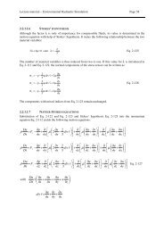
Examples of the structural and performance failures of a seadike are illustrated in Fig.1.<br />
The first figure shows over<strong>to</strong>pping of a dike. Depending on the overflow discharge and<br />
duration, this can be considered <strong>as</strong> a performance failure although no structural failure <strong>to</strong>ok<br />
place. In the second figure, erosion of a dike slope after a s<strong>to</strong>rm is depicted. This may be<br />
considered <strong>as</strong> a kind of structural failure since the cover layer of the dike w<strong>as</strong> not designed<br />
properly. However, this is not a performance failure since <strong>flood</strong>ing did not occur, although the<br />
probability of failure can be significantly higher than in the c<strong>as</strong>e of over<strong>to</strong>pping. The third<br />
figure shows a complete, both structural and performance failure of a dike.<br />
4
Fig.1. Example failures of a seadike (Kortenhaus et al., 2002).<br />
In relation <strong>to</strong> <strong>flood</strong> hazard, different failure types can be recognized (Table 3), all of them<br />
being described by the relationship: z = r – l < 0. However, the most common failure<br />
mechanism of new or well-maintained <strong>flood</strong> defence systems is over<strong>to</strong>pping of the structures,<br />
that is the performance failure.<br />
Table 3. Flood defence system failure types (Kortenhaus et al., 2002).<br />
Failure type Load, l Resistance, r Unit<br />
The <strong>flood</strong> water level, Z The structure crest level, Zd [m]<br />
The maximum <strong>flood</strong> discharge, Q The system design discharge, Qd [m 3 /s]<br />
The actual overflow The critical overflow [m 3 Over<strong>to</strong>pping*<br />
/s]<br />
The actual overflow velocity The critical overflow velocity [m/s]<br />
Breaching The actual <strong>flood</strong> duration The critical <strong>flood</strong> duration [h]<br />
Sliding The actual force The critical force [kN]<br />
Scouring The actual shear stress The critical shear stress [kPa]<br />
Tipping The actual moment The critical moment [kNm]<br />
Instability of<br />
revetment<br />
The actual force The critical force [kN]<br />
Infiltration The actual <strong>flood</strong> duration The critical <strong>flood</strong> duration [h]<br />
Seepage The actual hydraulic gradient The critical hydraulic gradient [/]<br />
* the performance failure<br />
5
3.2. Probability of failure of a <strong>flood</strong> defence system<br />
The failure of <strong>flood</strong> defence systems due <strong>to</strong> over<strong>to</strong>pping of <strong>flood</strong> defence structures is<br />
commonly expressed in terms of water and crest levels (Table 3), so that the performance<br />
function takes the form: z = Zd – Z. This simply means that, provided the performance failure<br />
only is considered, <strong>flood</strong>ing will take place if Z > Zd.<br />
However, <strong>flood</strong>ing is possible <strong>to</strong> occur even if Z ≤ Zd, when a structural failure occurs in<br />
an element of the <strong>flood</strong> defence system. Considering multiple possible types of the structural<br />
failure (Table 3), a relationship can be defined (Fig.2) between the probability of failure of the<br />
<strong>flood</strong> defence system (e.g. levee), P , and the <strong>flood</strong> water level, Z, along with the two<br />
f<br />
characteristic water levels (NRC, 2000):<br />
- the probable failure point (the level <strong>as</strong>sociated with a high probability of failure), Z o , and<br />
- the probable non-failure point (the level <strong>as</strong>sociated with a negligible probability of<br />
failure), Zo.<br />
Figure 2. Relationship between the probability of failure<br />
of the <strong>flood</strong> defence system (e.g. levee) and the <strong>flood</strong> water level.<br />
Accordingly, the following possibilities exist:<br />
- Pf = 0, if Z ≤ Zo;<br />
- 0 < Pf < 1, if Zo<br />
< Z ≤ Z o ; (5)<br />
- P = 1,<br />
o<br />
if Z > Z .<br />
f<br />
By definition, Zo represents the damage threshold, or resistance of the system.<br />
It is often <strong>as</strong>sumed, for simplicity, that Z o ≈ Zd.<br />
Obviously, P is a conditional probability, or a probability of exceedance of the damage<br />
f<br />
threshold, given a <strong>flood</strong> event with the maximum discharge Q and the corresponding water<br />
level Z. As a system is considered reliable unless it fails, the reliability and probability of<br />
failure sum <strong>to</strong> unity. So, the conditional reliability, or the conditional non-exceedance<br />
probability, is: = 1 – P .<br />
R f<br />
f<br />
The conditional probabilities can be defined for each type of failure, at any location along<br />
the river, or at the whole river section.<br />
6
For the event i, the conditional probability of a specified failure type j (e.g. overflowing)<br />
at any location x along the river, is:<br />
P i<br />
∫<br />
f , j,<br />
x ( ) = f z,<br />
j,<br />
x<br />
Ω<br />
Θ ( Θ)<br />
⋅ dΦ<br />
, (6)<br />
where:<br />
Θ – the input parameter space;<br />
Ω – the “failure region”, where the safety margin z is negative;<br />
Φ – the vec<strong>to</strong>r containing all the random variables considered.<br />
For a river section of the length X, the conditional probability of failure of the type j at the<br />
whole river section is:<br />
P<br />
f i<br />
( Θ)<br />
= f z,<br />
j,<br />
x ( Θ)<br />
⋅ dΦ<br />
dX<br />
. (7)<br />
, j ∫∫<br />
X Ω<br />
⋅<br />
For the whole system (river section having the length X and all the failure types<br />
considered, I), treated <strong>as</strong> a series system which fails when at le<strong>as</strong>t one section fails, the<br />
conditional probability of failure of the system (given a <strong>flood</strong> i of certain probability of<br />
occurrence) is:<br />
Pfi ∫∫∫<br />
( Θ)<br />
= f , , ( Θ)<br />
⋅ dΦ<br />
⋅dX<br />
⋅ dI<br />
. (8)<br />
I X Ω<br />
z j x<br />
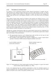
For a complex system involving many components and contributing random parameters, it<br />
is impracticable and often impossible <strong>to</strong> directly combine the uncertainties of the components<br />
and parameters <strong>to</strong> yield the system reliability. Instead, the system is subdivided according <strong>to</strong><br />
the failure types (or orher criteria), for which the component probabilities are first determined<br />
and then combined <strong>to</strong> give the system reliability (Yen and Tung, 1993). Fault tree <strong>analysis</strong> is<br />
a useful <strong>to</strong>ol for this purpose. Fault tree <strong>analysis</strong> is a backward <strong>analysis</strong> which begins with a<br />
system failure (e.g. <strong>flood</strong> dis<strong>as</strong>ter) and traces backward, searching for possible causes of the<br />
failure.<br />
A fault tree approach can be efficiently applied in <strong>analysis</strong> of multiple failure types (see<br />
the example in Kortenhaus et al., 2002). However, the independence of failure modes from<br />
each other should be carefully checked.<br />
The overall probability of failure of a <strong>flood</strong> defence system is given by a general<br />
relationship for description of the <strong>risk</strong> of natural hazards, illustrated in Fig.3 (Hollenstein,<br />
2005).<br />
Figure 3. A general relationship for description of the <strong>risk</strong> of natural hazards.<br />
This equation can also be expressed <strong>as</strong>:<br />
R = P(<br />
H)<br />
⋅ P(<br />
I H)<br />
⋅ P(<br />
E I)<br />
⋅ P(<br />
S E)<br />
⋅ S , (9)<br />
where:<br />
P (H ) – probability of hazard occurrence (occurrence of a hazardous event);<br />
7
P ( I H ) – probability of the hazard intensity (load), given the event;<br />
P ( E I)<br />
– probability of exposure <strong>to</strong> the hazard (or failure, or a consequence occurrence),<br />
given the intensity of the hazard (note that P ( E I)<br />
= P );<br />
P ( S E)<br />
– probability of a specific value of damage fac<strong>to</strong>r (or vulnerability, degree of loss,<br />
damage ratio), given the failure of defence system;<br />
S – the consequence.<br />
It should be noted that:<br />
- The probability of exposure <strong>to</strong> a hazard, P ( E I)<br />
, is a conditional probability! It is the<br />
probability that damage occurs (i.e. an object or a system is exposed <strong>to</strong> a hazard), given<br />
the occurrence of a hazard of a certain probability and intensity. Thus, the exposure <strong>to</strong><br />
hazard relates <strong>to</strong> the probability of consequence occurrence.<br />
- Human vulnerability <strong>to</strong> dis<strong>as</strong>ter contributes <strong>to</strong> the extent of the consequence itself.<br />
The probability of dis<strong>as</strong>ter occurrence, or the probability of consequence occurrence, PS,<br />
can be defined <strong>as</strong> the product of the probabilities (Fig.4):<br />
P = P(<br />
H ) ⋅ P(<br />
I H ) ⋅ P(<br />
E I ) = P(<br />
H ) ⋅ P(<br />
I H ) ⋅ P . (10)<br />
S<br />
Figure 4. Difference in definition of probabilities of<br />
hazard occurrence and dis<strong>as</strong>ter occurrence.<br />
The following variables are used in the c<strong>as</strong>e of <strong>flood</strong> hazard:<br />
H – the maximum discharge Q*<br />
of a particular <strong>flood</strong> event, having a probability of<br />
occurrence P*<br />
;<br />
I – any variable representing load, say the water level Z * , corresponding <strong>to</strong> the flow<br />
discharge Q*<br />
(Table 3);<br />
E – failure of the system (z < 0) due <strong>to</strong> the water level Z * (described by the condition:<br />
z = Zo – Z * < 0), or exceedance of the damage threshold,<br />
so that:<br />
R = P * ⋅P(<br />
Q * P * ) ⋅ P(<br />
Z * Q * ) ⋅ P[(<br />
Z o − Z*<br />
≤ 0)<br />
Z * ] ⋅ P[<br />
S * ( Z o − Z*<br />
≤ 0)<br />
] ⋅ S * , (11)<br />
142 4 43 4<br />
1444444442444444443<br />
or:<br />
P(<br />
Q*)<br />
f<br />
P(<br />
S*<br />
Z*<br />
)<br />
f<br />
8
*<br />
R = P * ⋅P(<br />
Q * P * ) ⋅ P(<br />
Z * Q * ) ⋅ Pf<br />
⋅ P[<br />
S * ( Z o − Z*<br />
≤ 0)<br />
] ⋅ S * , (12)<br />
142<br />
4 43 4<br />
1444<br />
4 244443<br />
and:<br />
*<br />
S<br />
P(<br />
Q*)<br />
P = P * ⋅P(<br />
Q * P * ) ⋅ P(<br />
Z * Q * ) ⋅ P<br />
14<br />
4 2443<br />
f<br />
P(<br />
Q*)<br />
*<br />
P(<br />
S*<br />
Z*<br />
)<br />
The probabilities describe the following uncertainties:<br />
. (13)<br />
P *<br />
- natural variability;<br />
P ( Q * P * ) - uncertainty in the discharge-probability relationship;<br />
P ( Z * Q * ) - uncertainty in the stage-discharge relationship;<br />
P[( Z o − Z*<br />
≤ 0)<br />
Z * ] - uncertainty in structural performance of defence system<br />
(uncertainty of damage threshold value);<br />
P[ S * ( Z o − Z*<br />
≤ 0)<br />
] - uncertainty in the stage-damage relationship.<br />
If no uncertainties are taken in<strong>to</strong> account, then:<br />
*<br />
R = PS<br />
⋅ S*<br />
= P * ⋅S<br />
* . (14)<br />
Therefore, the deterministic c<strong>as</strong>e can be defined <strong>as</strong>:<br />
*<br />
PS = P * , (15)<br />
*<br />
f =<br />
provided a <strong>flood</strong>ing <strong>to</strong>ok place ( P 1,<br />
or Z > Zd).<br />
If it is <strong>as</strong>sumed, for a moment, that there exist unique functions Q(P) and Z(Q), then:<br />
P ( Q * P * ) = 1,<br />
P ( Z * Q * ) = 1,<br />
and:<br />
*<br />
S<br />
*<br />
P = P * ⋅Pf<br />
. (16)<br />
Possibilities of performance of a <strong>flood</strong> defence system are shown in Table 4.<br />
Table 4. A possible performance of a <strong>flood</strong> defence system.<br />
C<strong>as</strong>e Performance P*<br />
Z* ≤ Zo no failure P* ≥ Po<br />
*<br />
P f<br />
*<br />
P f = 0<br />
*<br />
P S<br />
S<br />
*<br />
P S = 0 S = 0<br />
Zo < Z* ≤ Zd structural failure P* < Po 0 < P < 1 0 < P < P* S ≠ 0<br />
Z* > Zd performance failure P* < Po<br />
Po – the probability of occurrence of the water level Zo<br />
*<br />
f<br />
*<br />
P f = 1<br />
*<br />
S<br />
*<br />
P S = P* S ≠ 0<br />
If the performance failure only is considered, then it means that the system is <strong>as</strong>sumed <strong>to</strong><br />
perform perfectly well until the over<strong>to</strong>pping occurs, that is Zo = Zd, so that the two states only<br />
are possible (Table 5).<br />
9
Table 5. A possible performance of a <strong>flood</strong> defence system (the performance failure only is<br />
considered).<br />
C<strong>as</strong>e Performance P*<br />
Z ≤ Zd no failure P* ≥ Po<br />
Z > Zd failure P* < Po<br />
*<br />
P f<br />
*<br />
P f = 0<br />
*<br />
P f = 1<br />
*<br />
P S<br />
S<br />
*<br />
P S = 0 S = 0<br />
*<br />
P S = P* S ≠ 0<br />
Provided the expected damage Sj is defined for each type of failure j (having the<br />
probability of occurrence determined by Eq.7, then the expected damage Si<br />
having a<br />
P , j<br />
probability Pi can be estimated:<br />
S<br />
f i<br />
n<br />
n<br />
* * * *<br />
i = ∑ S j ⋅ Pfi<br />
, j , Pi<br />
= PS<br />
, i = Pi<br />
⋅ Pf<br />
≈ Pi<br />
⋅∑<br />
Pf<br />
j . (17)<br />
i<br />
i ,<br />
j=<br />
1<br />
j=<br />
1<br />
By weighing values of Sj (the expected damage due <strong>to</strong> a specific failure type) by the<br />
corresponding probabilities ( ), a more accurate estimate of Si<br />
can be provided (which is<br />
then <strong>to</strong> be used in Eq.3).<br />
P , j<br />
3.3. The procedure of <strong>flood</strong> damage <strong>as</strong>sessment<br />
f i<br />
A (socio-economic) system, exposed <strong>to</strong> a <strong>flood</strong>, is considered. Occurrence of a hazard<br />
results in an impact <strong>to</strong> the system, called load, which is proportional <strong>to</strong> the hazard intensity<br />
(i.e. the hazard magnitude and/or hazard duration). On the other hand, the exposure of the<br />
system <strong>to</strong> the hazard is an inverse function of the system resistance.<br />
The standard procedure of <strong>flood</strong> damage <strong>as</strong>sessment is illustrated in Fig.5. It should be<br />
noted that:<br />
- The hydrologic input is generally represented by the function Q(t), describing the whole<br />
wave of a <strong>flood</strong> having the probability of occurrence P(Q) = P*. For simplicity, the<br />
maximum flow discharge, hereinafter noted <strong>as</strong> Q*, is used for representation of the <strong>flood</strong><br />
wave.<br />
- The load l is a me<strong>as</strong>ure of intensity of the <strong>flood</strong> hazard, and is a function of the maximum<br />
flow discharge Q*. For an event under consideration, the load l can be represented by one<br />
or more hydraulic parameters (Table 3), obtained on the b<strong>as</strong>is of the flow simulation (flow<br />
depth or water stage, flow velocity, <strong>flood</strong> duration, <strong>flood</strong> water load such <strong>as</strong> sediment,<br />
salts, sewage, chemicals, etc.).<br />
- The set of all possible c<strong>as</strong>es of failure (for all the events causing the failure), defined by z<br />
< 0, is called failure region and accounts for failures due <strong>to</strong> different causes and at<br />
different places (i.e. river cross-sections) of the system. Obviously, the safety margin z is a<br />
me<strong>as</strong>ure of exposure <strong>to</strong> the hazard.<br />
- The expected annual damage, S , is calculated using Eq.3.<br />
- By this procedure, the uncertainty due <strong>to</strong> natural variability of flow is taken in<strong>to</strong> account.<br />
3.4. Flood damage <strong>as</strong>sessment under no uncertainty (damage due <strong>to</strong> performance failure only)<br />
The procedure is illustrated in Fig.6. In this figure, load (or hazard intensity) is<br />
represented by the water stage, which is a typical c<strong>as</strong>e in damage <strong>as</strong>sessment. In principle,<br />
any relevant parameter (Table 3) can be used in such an <strong>analysis</strong>, <strong>as</strong> well.<br />
10
Figure 5. The traditional <strong>flood</strong> damage <strong>as</strong>sessment procedure.<br />
Generally, the system resistance is described by the damage threshold Zo – the minimum<br />
water stage for which a <strong>flood</strong>ing takes place. In this c<strong>as</strong>e, the performance failure only, i.e.<br />
the so-called hydrologic hazard – failure of the system due <strong>to</strong> over<strong>to</strong>pping a protective<br />
structure, is considered, so that the damage threshold equals the crest level of the system<br />
structure (Zo = Zd). For Z > Zd, the resistance is smaller than the load (z < 0), which means that<br />
the system is exposed <strong>to</strong> <strong>flood</strong> and the damage will occur. The system vulnerability is<br />
represented by the stage-damage curve. The damage-exceedance probability relationship is<br />
referred <strong>to</strong> <strong>as</strong> the <strong>risk</strong> curve (Apel et al., 2004).<br />
11
Figure 6. Procedure of <strong>flood</strong> damage <strong>as</strong>sessment under no uncertainty<br />
(over<strong>to</strong>pping is the only failure type considered, that is Zo = Zd).<br />
3.5. Flood damage <strong>as</strong>sessment under uncertainty in structural performance<br />
Compared <strong>to</strong> the procedure illustrated in Fig.6, the <strong>analysis</strong> shown in Fig.7 is extended <strong>to</strong><br />
account for multiple failure types of a system under consideration, that is for the uncertainty<br />
in structural performance of the system. In this c<strong>as</strong>e, damage can occur not only for water<br />
levels Z > Zd, but also for those Zo < Z ≤ Zd. Consequently, a shaded area is added <strong>to</strong> the stagedamage<br />
curve. For levels Zo < Z ≤ Zd, a possibility of the structural failure exists (0 < Pf < 1),<br />
so that the probability of <strong>flood</strong>ing is 0 < Pf < P* and the S(Pf) function departs from S(P)<br />
curve. Depending on values of Pf, the departing part of the <strong>risk</strong> curve S(Pf) can take different<br />
shapes within the grey-coloured area, one possible shape being shown in the figure.<br />
There is obviously a difference in calculated values of the expected annual damage S in<br />
the two c<strong>as</strong>es (the purple-coloured are<strong>as</strong> in Fig.6 and Fig.7). If the uncertainty of structural<br />
performance is accounted for (Fig.7), <strong>flood</strong>ing occurs starting from a Zo ≤ Zd, which could<br />
cause an incre<strong>as</strong>e in S . However, the corresponding probabilities of <strong>flood</strong>ing are low due <strong>to</strong> a<br />
reliability of the system (see Pf in Table 4), thus causing a decre<strong>as</strong>e in S . It seems, on the<br />
b<strong>as</strong>is of recent investigations (Faber and Nachtnebel, 2002; Kortenhaus et al., 2002) that the<br />
overall effect of multiple failure types consideration is a decre<strong>as</strong>e in S compared <strong>to</strong> one<br />
failure-type (i.e. performance failure) c<strong>as</strong>e, which is a conservative estimate of <strong>flood</strong> damage.<br />
12
Figure 7. Procedure of <strong>flood</strong> damage <strong>as</strong>sessment<br />
under uncertainty in structural performance (Zo ≤ Zd).<br />
3.6. Flood damage <strong>as</strong>sessment under uncertainty<br />
Due <strong>to</strong> knowledge uncertainty, the <strong>risk</strong> <strong>as</strong>sessment always h<strong>as</strong> considerable margins of<br />
error, or error bounds (Plate, 1998). As a result of natural variability (both in space and time),<br />
the inputs of a system show random deviations. Being dependent on the random inputs and<br />
subject <strong>to</strong> knowledge uncertainty (including the uncertainty of structural performance), the<br />
outputs are not deterministic, but also show random variations. Therefore, there are<br />
uncertainty bounds of the functions described in Figs.6 and 7 (the discharge-probability,<br />
stage-discharge and damage-stage functions) and many possible realizations of the functions<br />
within the bounds (Fig.8). As stated by Petrakian et al. (1989), “the <strong>risk</strong> is not the mean of the<br />
<strong>risk</strong> curve, but rather the curve itself. If uncertainties due <strong>to</strong> our incomplete knowledge must<br />
be considered, then a whole family of curves might be needed <strong>to</strong> express the idea of <strong>risk</strong>.”<br />
As a result, the resistance (or the damage threshold), Zo, becomes a random variable<br />
(compare Figs.6 and 7 with Fig.8):<br />
- In the c<strong>as</strong>e of existing levees, the resistance is a random variable due <strong>to</strong> uncertainty of<br />
structural performance, although for well built and maintained structures, this uncertainty<br />
is considered rather low (Apel et al., 2004).<br />
- In the c<strong>as</strong>e of planning levees, the resistance is a random variable due <strong>to</strong> natural<br />
variability, model and parameter uncertainty, <strong>as</strong> well <strong>as</strong> that in structural performance.<br />
13
Figure 8. Procedure of <strong>flood</strong> damage <strong>as</strong>sessment under uncertainty.<br />
Accordingly, the expected annual damage becomes a random variable, <strong>to</strong>o - there are<br />
different values of the expected annual damage (shaded are<strong>as</strong>) with a different likeliness of<br />
occurrence.<br />
By choosing appropriate uncertainty bounds for the stage-damage function, it is possible<br />
<strong>to</strong> cover the uncertainty in structural performance by this function (NRC, 2000).<br />
There are several approaches that can be applied in uncertainty <strong>analysis</strong>:<br />
1. Deterministic approach (Fig.6), which takes in<strong>to</strong> account the natural variability and<br />
disregards the knowledge uncertainty. All (input and output) parameters are described by<br />
single values. The effect of uncertainty of the input parameters can be <strong>as</strong>sessed by<br />
performing a sensitivity <strong>analysis</strong> (Oberguggenberger, 2005a) and <strong>analysis</strong> of different<br />
scenarios, a so-called “what if” method (Yoe, 1994). The results are typically reported <strong>as</strong> a<br />
single, most likely value (the point-estimate), or three values (the three-point estimate),<br />
such <strong>as</strong> the minimum likely value, the maximum likely value and the most likely value<br />
(Walsh and Moser, 1994), or a “bare estimate”, a “conservative estimate” and a “worstc<strong>as</strong>e<br />
estimate” (Rowe, 1994), where the estimates are performed by subjective judgment.<br />
2. Interval <strong>analysis</strong>, which handles a whole range of values of a variable. The uncertainty of<br />
a parameter is described by an interval, defining bounds in terms of a worst- and best-c<strong>as</strong>e<br />
<strong>as</strong>sumptions. Input parameters are varied over a specified range of values and a range of<br />
output values is determined. However, the range of values is often subjectively<br />
determined and it is presumed that the appropriate range of values is identified and all<br />
14
values in that range are equally likely. Although the <strong>to</strong>tal variability of the parameters can<br />
be captured, no detailed information on the uncertainty is provided.<br />
3. Probabilistic approach, in which the uncertainty is described in the most informative, but<br />
also the most strict way – by means of probability. Input parameters are treated <strong>as</strong> random<br />
variables with known probability distributions, and the result is a probability distribution<br />
of an output parameter. However, disadvantages of this approach have been identified in<br />
many engineering applications, such <strong>as</strong>:<br />
- it generally requires much input data, often more than can be provided, so that<br />
choosing a distribution and estimating its parameters are the critical fac<strong>to</strong>rs<br />
(Ossenbruggen, 1994);<br />
- it requires that probabilities of events considered have <strong>to</strong> sum up <strong>to</strong> 1; therefore, when<br />
additional events are taken in<strong>to</strong> consideration, the probabilities of events change;<br />
- probabilities have <strong>to</strong> be set up in a consistent way and thus do not admit incorporating<br />
conflicting information (which could make confusion about the statistical independence<br />
of events).<br />
4. Alternative approaches, b<strong>as</strong>ed on the “imprecise probability”, in which some axioms of<br />
probability theory are relaxed (Oberguggenberger, 2005a; Oberguggenberger and Fellin,<br />
2005):<br />
4.1. Fuzzy set approach, in which the uncertainty is described <strong>as</strong> a family of intervals<br />
parametrized in terms of the degree of possibility that a parameter takes a specified<br />
value. This approach admits much more freedom in modelling (for example, it is<br />
possible <strong>to</strong> mix fuzzy numbers with relative frequencies or his<strong>to</strong>grams), and may be<br />
used <strong>to</strong> model vagueness and ambiguity. It is useful when no sufficient input data is<br />
available.<br />
4.2. Random set approach, in which the uncertainty is described by a number of intervals,<br />
focal sets, along with their corresponding probability weights. For example, the focal<br />
sets may be estimates given by different experts and the weights might correspond <strong>to</strong><br />
relative credibility of each expert. The probability weight could be seen <strong>as</strong> the relative<br />
frequency (his<strong>to</strong>gram), however the difference is that the focal sets may overlap. This<br />
is the most general approach – every interval, every his<strong>to</strong>gram, and every fuzzy set can<br />
be viewed <strong>as</strong> a random set.<br />
The probabilistic and fuzzy approaches <strong>to</strong> uncertainty <strong>analysis</strong> in <strong>flood</strong> <strong>risk</strong> <strong>as</strong>sessment<br />
will be described in the following text.<br />
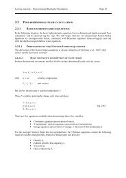
3.6.1. Probabilistic approach<br />
The main objective of the probabilistic approach <strong>to</strong> <strong>risk</strong> <strong>as</strong>sessment is <strong>to</strong> describe the<br />
uncertainties of input parameters in terms of probabilities (Fig.9), in order <strong>to</strong> define a<br />
probability distribution of the output, that is, of the expected annual damage (Fig.10).<br />
Different me<strong>as</strong>ures exist <strong>to</strong> describe the degree of uncertainty of a parameter, function, a<br />
model, or a system (Tung and Yen, 1993):<br />
- The probability density function (PDF) of the quantity subject <strong>to</strong> uncertainty. It is the most<br />
complete description of uncertainty. However, in most practical problems such a function<br />
can not be derived or found precisely.<br />
- A reliability domain, such <strong>as</strong> the confidence interval. The related problems include that:<br />
1. the parameter population may not be normally distributed <strong>as</strong> usually <strong>as</strong>sumed;<br />
2. there are no means <strong>to</strong> combine directly the confidence intervals of random input<br />
15
variables <strong>to</strong> give the confidence interval of the output.<br />
- Statistical moments of the random variable. For example, the second moment is a me<strong>as</strong>ure<br />
of dispersion of a random variable.<br />
Figure 9. Probabilistic approach <strong>to</strong> uncertainty <strong>analysis</strong>.<br />
Figure 10. Probability density function of the expected annual damage.<br />
16
There are the following methods of probabilistic uncertainty <strong>analysis</strong> (Yen and Tung,<br />
1993):<br />
- Analytical methods, deriving the PDF of model output analytically <strong>as</strong> a function of the<br />
PDFs of input parameters.<br />
- Approximation methods (or parameter estimation methods):<br />
1. methods of moments (e.g. first-order second-moment methods, second-order method);<br />
2. simulation or sampling (e.g. Monte Carlo simulation);<br />
3. integral transformation techniques (Fourier transform, Laplace transform).<br />
Theoretically, the statistical moments can be obtained by integrating the performance<br />
function with the distribution range of the random input variables. In practice, the integration<br />
is usually approximated using point-estimate methods, Taylor series approximations or<br />
simulation methods (Leggett, 1994). In these methods, probability distributions of the random<br />
variables are replaced by means and standard deviations of the random variables. The<br />
approximate integration is achieved by performing repetitive, deterministic analyses using<br />
various possible combinations of values of the random variables.<br />
Some of the methods, relevant for <strong>flood</strong> <strong>risk</strong> <strong>as</strong>sessment, will be described in the<br />
following text.<br />
It should be noted that:<br />
- Indices of S refer <strong>to</strong> probability of exceedance (95%, 50%, and 5%), and the probability<br />
density function (Fig.10) is related <strong>to</strong> probability of non-exceedance (the corresponding<br />
values being 5%, 50%, and 95%, respectively).<br />
- The expectation of S reflects only natural variability, the probability distribution of S<br />
(Fig.10) reflects only knowledge uncertainty (NRC, 2000).<br />
- The uncertainty in structural performance can be included in the stage-damage curve or<br />
can be introduced in the simulation <strong>as</strong> an independent function connecting the conditional<br />
probability of failure, Pf, with the probability of hazard occurrence, P* (NRC, 2000). In<br />
the latter c<strong>as</strong>e, it is necessary <strong>to</strong> calculate the overall probability of failure, Pf, using Eq.8.<br />
Direct integration. Due <strong>to</strong> complexity of the problem depicted in Fig.9, it is very difficult <strong>to</strong><br />
obtain the PDF of the S analitically. The method of direct integration can be successfully<br />
used in determining the conditional probability of failure, Pf.<br />
The problem is <strong>to</strong> estimate the probability density function of the system output, fz(z), if<br />
resistance and load are represented by probability density functions, fr(r) and fl(l) (Fig.11).<br />
Figure 11. Probability density functions of resistance and load.<br />
17
In a general c<strong>as</strong>e, the function fl(l) overlaps fr(r) <strong>to</strong> some extent, due <strong>to</strong> variances of both<br />
functions (<strong>as</strong> a result of uncertainties). This indicates a possibility that load may exceed<br />
resistance of the system (r – l < 0), even though the expected value of resistance is greater<br />
than the expected value of load, E( r)<br />
− E(<br />
l)<br />
> 0.<br />
The probability density function of safety margin, fz(z), is a useful means for analyzing<br />
reliability of a system (Fig.12). In c<strong>as</strong>e the function fl(l) overlaps fr(r), <strong>as</strong> shown in Fig.11, a<br />
part of the function fz(z) extends <strong>to</strong> the region where z < 0 (Fig.12).<br />
Figure 12. Probability density function of safety margin.<br />
The probability density function of the safety margin provides an explicit characterization<br />
of expected system performance. As mentioned before, failure of a system (which refers <strong>to</strong><br />
any occurrence of an adverse event under consideration), takes place if z < 0. So, the<br />
probability of failure given the load l, Pf, , can be expressed <strong>as</strong>:<br />
0<br />
P = P{<br />
z ≤ } = ∫ f z<br />
−∞<br />
f 0 ( z)<br />
⋅ dz<br />
, (18)<br />
and the probability of success (reliability) of the system (or the probability that the system<br />
will not be exposed <strong>to</strong> hazard), Rf, <strong>as</strong>:<br />
{ z > 0}<br />
= f z ( z)<br />
⋅ dz<br />
= 1 Pf<br />
R f = P ∫<br />
−<br />
∞<br />
0<br />
. (19)<br />
If r and l are <strong>as</strong>sumed <strong>to</strong> follow the normal probability distribution, then z is also normally<br />
distributed, and the functions fr(r), fl(l) and fz(z) can be described by a well-known formula,<br />
which, for the safety margin z, h<strong>as</strong> the following form:<br />
f<br />
z<br />
[ z−E<br />
( z)]<br />
−<br />
2⋅σ<br />
2<br />
1<br />
2<br />
z<br />
( z)<br />
= ⋅ e , (20)<br />
σ ⋅ 2π<br />
z<br />
A parameter of the distribution, σz (standard deviation of z), can be defined <strong>as</strong>:<br />
z<br />
2<br />
r<br />
2<br />
l<br />
σ = σ + σ − 2 ⋅ r ⋅ σ<br />
r<br />
⋅ σ<br />
l<br />
, (21)<br />
18
where σr and σl – standard deviations of r and l, respectively; r – correlation coefficient,<br />
−1≤r ≤+ 1 (if r and l are not correlated, r = 0).<br />
Another parameter of the distribution, E(z<br />
) (expected value of z), depends on the<br />
formulation of z (Yen and Tung, 1993):<br />
1. z = r – l (then E( z)<br />
= E(<br />
r)<br />
− E(<br />
l)<br />
);<br />
2. z = f – 1 ;<br />
3. z = ln f ,<br />
where f is the fac<strong>to</strong>r of safety:<br />
r<br />
f =<br />
l<br />
lower<br />
upper<br />
E(<br />
r)<br />
− nr<br />
⋅ σ<br />
=<br />
E(<br />
l)<br />
+ n ⋅ σ<br />
l<br />
r<br />
l<br />
, (22)<br />
where rlower – conservative estimate of the resistance, lupper – liberal estimate of the load, nc<br />
and nd – sigma units for resistance and load, respectively, or:<br />
f fc<br />
E(<br />
r)<br />
E(<br />
l)<br />
= = , (23)<br />
where fc is the central fac<strong>to</strong>r of safety.<br />
The major limitation of using fc is that variance of the distributions is not considered.<br />
Therefore, the preferred procedure is <strong>to</strong> use the fac<strong>to</strong>r of safety according <strong>to</strong> Eq.22, which<br />
reduces the resistance <strong>as</strong> a function of the standard deviation in order <strong>to</strong> obtain a conservative<br />
estimate of the resistance, and a higher than average load is used <strong>to</strong> define a worst-c<strong>as</strong>e<br />
condition.<br />
It is useful <strong>to</strong> address the following equivalencies, which exist between the terms used in<br />
reliability engineering and cost-benefit analyses:<br />
safety margin = benefit – cost = the net benefit<br />
central fac<strong>to</strong>r of safety = benefit / cost = the cost-effectiveness<br />
Method of moments (first-order second-moment methods). The first-order second-moment<br />
method estimates uncertainty in terms of the variance of system output using variances of<br />
contributing fac<strong>to</strong>rs. The load and resistance functions are expanded in Taylor series at a<br />
reference point (about the expected values of input variables) and the second and higher-order<br />
terms in the series expansion are truncated, resulting in an approximation involving only the<br />
first two statistical moments of the variables (the expected value and the standard deviation).<br />
This simplification greatly enhances the practicality of the method because it is often<br />
difficult <strong>to</strong> find the PDF of the variable and relatively simple <strong>to</strong> estimate the first two<br />
statistical moments – either by calculating them from data, or by estimating them from<br />
experience (USACE, 1995b).<br />
Once the expected value and variance of z are estimated, an another useful indica<strong>to</strong>r of<br />
system performance, the reliability index, can be defined <strong>as</strong>:<br />
β = E( z)<br />
σ . (24)<br />
z<br />
It is a me<strong>as</strong>ure of the distance between the expected value of z and the limit state z = 0 (the<br />
number of standard deviations by which the expected value of a normally distributed<br />
performance function exceeds zero). It is a me<strong>as</strong>ure of reliability of an engineering system<br />
19
that reflects both mechanics of the problem and the uncertainty in the input variables.<br />
Formally, it is not necessary <strong>to</strong> <strong>as</strong>sume or determine the shape of the probability function<br />
(which is necessary <strong>to</strong> calculate an exact value of the probability of achieving the limit state),<br />
<strong>to</strong> be able <strong>to</strong> define the reliability index. Values of the reliability index are not absolute<br />
me<strong>as</strong>ures of probability, but are used <strong>as</strong> a relative me<strong>as</strong>ure of reliability or confidence in the<br />
ability of a structure <strong>to</strong> perform its function in a satisfac<strong>to</strong>ry manner.<br />
The probability of failure, <strong>as</strong>sociated with the reliability index, is a probability per<br />
structure – it h<strong>as</strong> no time-frequency b<strong>as</strong>is. Once a structure is constructed or loaded <strong>as</strong><br />
modelled, it either performs satisfac<strong>to</strong>rily or not (USACE, 1995b).<br />
It is noted that, especially for low probability events, the probability of failure is a rather<br />
poor indica<strong>to</strong>r of performance. In these c<strong>as</strong>es, the <strong>risk</strong> is an important additional indica<strong>to</strong>r<br />
(Plate, 1993).<br />
Simulation (Monte Carlo simulation). The most commonly used procedure for <strong>risk</strong><br />
<strong>as</strong>sessment under uncertainty is Monte Carlo simulation. It h<strong>as</strong> been succesfully applied in<br />
<strong>flood</strong> <strong>risk</strong> analyses (Moser, 1994; Faber and Nachtnebel, 2002; Kortenhaus et al., 2002; Apel<br />
et al., 2004).<br />
Monte Carlo simulation is a method <strong>to</strong> estimate the statistical properties of a random<br />
variable that is related <strong>to</strong> a number of random variables which may or may not be correlated<br />
(Yen and Tung, 1993). The method is useful when the direct calculation of probability<br />
functions is complicated (Ossenbruggen, 1994). The values of s<strong>to</strong>ch<strong>as</strong>tic input parameters<br />
(random numbers) are generated according <strong>to</strong> their distributional properties (i.e. <strong>to</strong> the<br />
specifed probability laws). Theoretically, each uncertain parameter can be introduced <strong>as</strong> a<br />
random number (Faber and Nachtnebel, 2002). The input probability distributions are<br />
repeatedly sampled in order <strong>to</strong> derive the PDF of the output. Expressing uncertainty in terms<br />
of probability distributions is an essential step (Yoe, 1994).<br />
The input required for performing the simulation are the means and standard deviations<br />
for the input variables (flow discharge, water stage and <strong>flood</strong> damage, see Fig.9). As<br />
mentioned before, the means and standard deviations <strong>as</strong> a me<strong>as</strong>ure of uncertainty can be<br />
quantified through statistical <strong>analysis</strong> of existing data, or judgmentally <strong>as</strong>signed (USACE,<br />
1995b). For example, for the purpose of uncertainty <strong>analysis</strong> in <strong>flood</strong> <strong>risk</strong> <strong>as</strong>sessment,<br />
recommendations on standard deviations of flow-frequency, flow-stage and damage-stage<br />
functions can be found in literature (Davis and Burnham, 1994; Moser, 1994).<br />
The Monte Carlo simulation routine randomly samples a discharge over a range of<br />
frequencies and within the confidence bands of the discharge-frequency curve. At that<br />
discharge, the routine then samples between the upper and lower confidence bands of the<br />
stage-discharge curve and randomly chooses a stage. At that stage, the routine samples<br />
between the upper and lower confidence bands of the stage-damage relationship and chooses<br />
a corresponding damage. This process is repeated until a statistically representative sample is<br />
developed.<br />
The Monte Carlo simulation can be applied for estimating the conditional probability of<br />
failure of a <strong>flood</strong> defence system, <strong>as</strong> well. In this c<strong>as</strong>e, the generated input parameter values<br />
are used <strong>to</strong> compute the value of the performance function z. After a large number of<br />
simulated realizations of z are generated, the reliability of the structure can be estimated by<br />
computing the ratio of number of realizations with z ≥ 0 <strong>to</strong> the <strong>to</strong>tal number of simulated<br />
realizations. This procedure enables all possible failure modes <strong>to</strong> be considered (Kortenhaus<br />
et al., 2002).<br />
A detailed description of the procedure can be found in literature (USACE, 1996c; NRC,<br />
2000). An example is given in Appendix, at the end of this document.<br />
20
Conclusions. The main features of the probabilistic approach are the following:<br />
- Knowledge uncertainty is quantified and explicitly included in evaluating project<br />
performance and benefit (USACE, 1995b);<br />
- This approach allows for several types of failures of the system <strong>to</strong> be considered, provided<br />
the safety margin of each of them is represented by a specific probability density function;<br />
- Each uncertain parameter can be introduced in<strong>to</strong> <strong>analysis</strong> by means of their probability<br />
distributions.<br />
- The actual probability of failure or reliability is used <strong>as</strong> a me<strong>as</strong>ure of performance of a<br />
system, rather than some empirical rule (Plate, 1993; Davis and Burnham, 1994).<br />
- Engineering and economic performance of a project can be expressed in terms of<br />
probability distributions (USACE, 1996a),<br />
- The following indica<strong>to</strong>rs of engineering performance can be determined (USACE, 1995c,<br />
1996c): the expected annual exceedance probability, the expected lifetime exceedance<br />
probability (or long-term <strong>risk</strong>), the conditional annual probability of non-exceedance,<br />
given the occurrence of an event.<br />
- A solid datab<strong>as</strong>e is required in order <strong>to</strong> perform a probabilistic <strong>analysis</strong>. An example is<br />
illustrated in a paper by Mai and von Lieberman (2000), where two internet-b<strong>as</strong>ed atl<strong>as</strong>es,<br />
containing a collection of hydraulic loads and information on resistance of protection<br />
structures (including the information on land use of the protected area), were used <strong>as</strong> a<br />
source for <strong>analysis</strong> of different scenarios of failure of the system.<br />
Deterministic approach. It can be concluded that the deterministic approach is a special c<strong>as</strong>e<br />
of the probabilistic one, for which:<br />
- No (knowledge) uncertainty is taken of the discharge-probability curve ( P ( Q * P * ) = 1).<br />
The expected value of discharge, E(Q), is used, given the probability of occurrence.<br />
- No uncertainty is taken of the stage-discharge curve ( P ( Z * Q * ) = 1).<br />
Consequently, the<br />
expected value of the water stage, E(Z), is used, given the flow discharge.<br />
- No uncertainty in structural performance is taken in<strong>to</strong> account (Zo = Z o = Zd). The only<br />
failure mode considered is the hydrologic hazard. This is b<strong>as</strong>ed on a simplified concept<br />
that the <strong>flood</strong> defence system will fail (Pf = 1) only in c<strong>as</strong>e of occurrence of the water<br />
levels Z > Zd, due <strong>to</strong> over<strong>to</strong>pping of the protective structure, where<strong>as</strong> it will work perfectly<br />
well (Pf = 0) during more frequent <strong>flood</strong> events, Z < Zd. As a result, the expected value of<br />
resistance, E(Zd), is used, given the water level Z. The system resistance is a deterministic<br />
quantity.<br />
- Finally, the expected value of the safety margin, E(z), is used, with no regard <strong>to</strong> its<br />
probability distribution. So, the user of numerical models does not know how large the<br />
safety margin of the deterministic results is. In other words, the probability of failure of<br />
the system, Pi, which is used in design, is b<strong>as</strong>ed on the expected values of resistance and<br />
load, with no regard of their variances (distributions). However, even if the E( r)<br />
− E(<br />
l)<br />
><br />
0, there is still a chance for r – l < 0 (for failure <strong>to</strong> occur), if the functions pz(r)<br />
and pz(l)<br />
overlap <strong>to</strong> some extent (Figs.11 and 12).<br />
- No uncertainty is taken of the stage-damage curve ( P ( S * Z * ) = 1).<br />
Consequently, the<br />
expected value of damage, E(S), is used, given the <strong>flood</strong> water level.<br />
-<br />
*<br />
The probability P (i.e. P ) of occurrence of a consequence (of the damage Si),<br />
is taken<br />
i<br />
S ,i<br />
equal <strong>to</strong> the probability of occurrence of a <strong>flood</strong>, P*, which will cause the over<strong>to</strong>pping<br />
(see Eqs.14 and 15). Hence, this approach is b<strong>as</strong>ed on an implicit <strong>as</strong>sumption that every<br />
hazard will create a consequence (i.e. hazard = dis<strong>as</strong>ter). In practice, it means that a<br />
probability of a <strong>flood</strong> event is adopted a priori, and the corresponding consequence<br />
21
(damage) is <strong>as</strong>sessed (NRC, 2000). However, the probability of consequence may be<br />
higher (or lower) due <strong>to</strong> the uncertainty. For example, if a levee is designed on the b<strong>as</strong>is of<br />
the 100-year <strong>flood</strong> event, a probability exists that failure will take place on occurrence of<br />
the very same (or even lesser) <strong>flood</strong> event (e.g. due <strong>to</strong> inaccurate estimate of probability of<br />
occurrence of the design <strong>flood</strong> event, due <strong>to</strong> dike-breach, etc.).<br />
- The output from the calculations is a composite of <strong>as</strong>sumed re<strong>as</strong>onable and worst-c<strong>as</strong>e<br />
values, which does not provide any illustration of the probabilistic density function of the<br />
output, pz(z). Estimates of variables, fac<strong>to</strong>rs and parameters are considered the “most<br />
likely” values (USACE, 1996a). However, there is no indication on the probability that<br />
the calculated expected annual damages will not be exceeded (NRC, 2000).<br />
Traditionally, the uncertainty is considered (Davis and Burnham, 1994):<br />
- by application of professional judgment<br />
- conducting sensitivity <strong>analysis</strong><br />
- by the addition of freeboard (in the c<strong>as</strong>e of levees/<strong>flood</strong> walls).<br />
This problem is conventionally overcome by developing conservative designs, using a<br />
safety fac<strong>to</strong>r (USACE, 1995b). For instance, when constructing a levee, a freeboard is added<br />
<strong>to</strong> the design water level, which accounts for all influences and uncertainties neglected by the<br />
model. An alternative is <strong>to</strong> define the actual safety level, and use it, instead of the design<br />
safety level, <strong>to</strong> determine Pi. The actual safety level is obtained by multiplying the design<br />
safety with reduction fac<strong>to</strong>rs, which account for the following fac<strong>to</strong>rs (van der Vat et al.,<br />
2001): the quality of the design and construction of the dike, its maintenance, chance of<br />
failure of operation of essential structures, reduced capacity of the river section due <strong>to</strong><br />
sedimentation, etc.<br />
The safety concept h<strong>as</strong> short-comings <strong>as</strong> a me<strong>as</strong>ure of the relative reliability of a system<br />
for different performance modes. A primary defficiency is that parameters must be <strong>as</strong>signed<br />
single values, although the appropriate values may be uncertain. The safety fac<strong>to</strong>r thus reflects<br />
(USACE, 1995b):<br />
- the condition of the feature;<br />
- the engineer´s judgment;<br />
- the degree of conservatism incorporated in<strong>to</strong> the parameter values.<br />
From the standpoint of the engineering performance, the freeboard approach provides<br />
(NRC, 2000):<br />
- inconsistent degrees of <strong>flood</strong> protection <strong>to</strong> different communities, and<br />
- different levels of protection in different regions.<br />
Nevertheless, there are still several advantages of the deterministic approach:<br />
- simplicity (avoiding the issue of dealing with probabilistic evaluations),<br />
- level of <strong>risk</strong> acceptability is implied within engineering standards,<br />
- legal liability is clear,<br />
- cost-effectiveness in terms of project study costs.<br />
For these re<strong>as</strong>ons, it is still commonly used in practice.<br />
22
3.6.2. Fuzzy set approach<br />
Several shortcomings have been identified in the probabilistic approach <strong>to</strong> <strong>risk</strong> <strong>as</strong>sessment<br />
and the formulation of the expected annual damage (Bogardi and Duckstein, 2003):<br />
- the <strong>analysis</strong> of low-failure-probability/high-consequence events may be misrepresented by<br />
the expected value;<br />
- the selection of the probability distribution, the two PDF’s, is often arbitrary, while results<br />
may be sensitive <strong>to</strong> this choice;<br />
- statistical data on load and resistance are often lacking;<br />
- the consequence functions are often quite uncertain;<br />
- the covariances among the various types of loads and resistances and the parameters<br />
involved in their estimation are commonly unknown; the results are, again, highly<br />
sensitive in this respect.<br />
Obviously, the probabilistic formulation may have difficulties when no sufficient<br />
statistical data are available (Bogardi and Duckstein, 2003). However, the size of the sample<br />
of data is commonly small and the data are often augmented by prior expert knowledge<br />
(Oberguggenberger and Russo, 2005). This necessitates the development of more flexible<br />
<strong>to</strong>ols for <strong>as</strong>sessing and processing subjective knowledge and expert estimates (Fetz, 2005;<br />
Fetz et al., 2005; Oberguggenberger, 2005b).<br />
In such a c<strong>as</strong>e, the fuzzy set formulation appears <strong>to</strong> be a practical alternative having a<br />
number of advantages:<br />
- fuzzy sets and fuzzy numbers may be used <strong>to</strong> characterize input uncertainty whenever<br />
variables (and/or relationships) are not defined precisely;<br />
- fuzzy arithmetic is considerably simpler and more manageable than the algebra of random<br />
numbers (Ganoulis et al., 1991);<br />
- fuzzy set <strong>analysis</strong> can be used with very few and weak prerequisite <strong>as</strong>sumptions (if<br />
hypotheses are considerably weaker than those of the probability theory);<br />
- in probability theory, functions of random variables are again random variables; in fuzzy<br />
set theory, computability is guaranteed.<br />
A detailed description of the procedure can be found in Appendix, at the end of this<br />
document.<br />
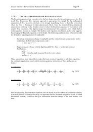
The procedure of <strong>flood</strong> damage <strong>as</strong>sessment under uncertainty, b<strong>as</strong>ed on the fuzzy set<br />
approach, is schematically illustrated in Figs.13 and 14.<br />
Several illustrative examples of application of the fuzzy set approach <strong>to</strong> <strong>risk</strong> <strong>as</strong>sessment<br />
and reliability <strong>analysis</strong> can be recommended:<br />
- groundwater contamination (Bogardi et al., 1989);<br />
- water resources and environmental engineering (Ganoulis et al., 1991);<br />
- <strong>flood</strong> management (Bogardi and Duckstein, 2003).<br />
23
Figure 13. Fuzzy set approach <strong>to</strong> uncertainty <strong>analysis</strong>.<br />
Figure 14. Membership function of the expected annual damage.<br />
24
4. References<br />
Apel, H., Thieken, A.H., Merz, B., Blöschl, G., 2004, Flood <strong>risk</strong> <strong>as</strong>sessment and <strong>as</strong>sociated<br />
uncertainty, Natural Hazards and Earth System Sciences, European Geosciences Union,<br />
Vol.4, 295-308.<br />
Bogardi, I., Duckstein, L., 1989, <strong>Uncertainty</strong> in environmental <strong>risk</strong> <strong>analysis</strong>, in: Risk <strong>analysis</strong><br />
and management of natural and man-made hazards, Haimes, Y.Y. and Stakhiv, E.Z.<br />
(Ed.), ASCE, 154-174.<br />
Bogardi, I., Duckstein, L., 2003, The fuzzy logic paradigm of <strong>risk</strong> <strong>analysis</strong>, in: Risk-b<strong>as</strong>ed<br />
decision making in water resources X, Haimes, Y.Y., Moser. D.A., Stakhiv, E.Z., (Eds.),<br />
ASCE, 12-22.<br />
Davis, D., Burnham, M.W., 1994, Risk-b<strong>as</strong>ed <strong>analysis</strong> for <strong>flood</strong> damage reduction, in: Riskb<strong>as</strong>ed<br />
decision making in water resources VI, Haimes, Y.Y., Moser. D.A., Stakhiv, E.Z.,<br />
(Eds.), ASCE, 194-200.<br />
Faber, R., Nachtnebel, H.-P., 2002, Flood <strong>risk</strong> <strong>as</strong>sessment in urban are<strong>as</strong>: development and<br />
application of a s<strong>to</strong>ch<strong>as</strong>tic hydraulic <strong>analysis</strong> method considering multiple failure types,<br />
in: Proceedings of the Second Annual IIASA-DPRI Meeting, Integrated Dis<strong>as</strong>ter Risk<br />
Management, Linnerooth-Bayer, J. (Ed.), Laxenburg, Austria, 8 pp.<br />
Fetz, T., 2005, Multi-parameter models: rules and computational methods for combining<br />
uncertainties, in: Analyzing <strong>Uncertainty</strong> in Civil Engineering, Fellin, W., Lessmann, H.,<br />
Oberguggenberger, M., Vieider, R. (Eds.), Springer, Berlin, Germany, 73-99.<br />
Fetz, T., Jäger, J., Köll, D., Krenn, G., Lessmann, H., Oberguggenberger, M., Stark, R.F.,<br />
2005, Fuzzy models in geotechnical engineering and construction management, in:<br />
Analyzing <strong>Uncertainty</strong> in Civil Engineering, Fellin, W., Lessmann, H., Oberguggenberger,<br />
M., Vieider, R. (Eds.), Springer, Berlin, Germany, 211-239.<br />
Ganoulis, J., Duckstein, L., Bogardi, I., 1991, Risk <strong>analysis</strong> of water quantity and quality<br />
problems: the engineering approach, in: Water resources engineering <strong>risk</strong> <strong>as</strong>sessment,<br />
Ganoulis, J., (Ed.), NATO ASI Series, Vol.629, Springer, 3-17.<br />
Hollenstein, K., 2005, Reconsidering the <strong>risk</strong> <strong>as</strong>sessment concept: Standardizing the impact<br />
description <strong>as</strong> a building block for vulnerability <strong>as</strong>sessment, Natural Hazards and Earth<br />
System Sciences, European Geosciences Union, Vol.5, 301-307.<br />
Kortenhaus, A., Oumeraci, H., Weissmann, R. Richwien, W., 2002, Failure mode and fault<br />
tree <strong>analysis</strong> for sea and estuary dikes, Proc. International Conference on Co<strong>as</strong>tal<br />
Engineering (ICCE), No.28, Cardiff, Wales, UK, 13 pp.<br />
Leggett, M.A., 1994, Reliability-b<strong>as</strong>ed Assessment of Corps Structures, in: Risk-b<strong>as</strong>ed<br />
decision making in water resources VI, Haimes, Y.Y., Moser. D.A., Stakhiv, E.Z., (Eds.),<br />
ASCE, 73-81.<br />
Mai, S., von Lieberman, N., 2000, Internet-b<strong>as</strong>ed <strong>to</strong>ols for <strong>risk</strong> <strong>as</strong>sessment for co<strong>as</strong>tal are<strong>as</strong>,<br />
Proc. of the 4 th Int. Conf. On Hydroinformatics, Iowa, USA.<br />
Moser, D.A., 1994, Quantifying <strong>flood</strong> damage uncertainty, in: Risk-b<strong>as</strong>ed decision making in<br />
water resources VI, Haimes, Y.Y., Moser. D.A., Stakhiv, E.Z., (Eds.), ASCE, 194-200.<br />
NRC (National Research Council), 2000, Risk Analysis and <strong>Uncertainty</strong> in Flood Damage<br />
Reduction Studies, National Academy Press, W<strong>as</strong>hing<strong>to</strong>n, D.C., 202 pp.<br />
Oberguggenberger, M., 2005a, The mathematics of uncertainty: models, methods and<br />
interpretations, in: Analyzing <strong>Uncertainty</strong> in Civil Engineering, Fellin, W., Lessmann, H.,<br />
Oberguggenberger, M., Vieider, R. (Eds.), Springer, Berlin, Germany, 51-72.<br />
Oberguggenberger, M., 2005b, Queueing models with fuzzy data in construction<br />
management, in: Analyzing <strong>Uncertainty</strong> in Civil Engineering, Fellin, W., Lessmann, H.,<br />
Oberguggenberger, M., Vieider, R. (Eds.), Springer, Berlin, Germany, 197-210.<br />
25
Oberguggenberger, M., Fellin, W., 2005, The fuzziness and sensitivity of failure probabilities,<br />
in: Analyzing <strong>Uncertainty</strong> in Civil Engineering, Fellin, W., Lessmann, H., Oberguggenberger,<br />
M., Vieider, R. (Eds.), Springer, Berlin, Germany, 33-49.<br />
Oberguggenberger, M., Russo, F., 2005, Fuzzy, probabilistic and s<strong>to</strong>ch<strong>as</strong>tic modelling of an<br />
el<strong>as</strong>tically bedded beam, in: Analyzing <strong>Uncertainty</strong> in Civil Engineering, Fellin, W.,<br />
Lessmann, H., Oberguggenberger, M., Vieider, R. (Eds.), Springer, Berlin, Germany, 183-<br />
196.<br />
Ossenbruggen, P.J., 1994, Fundamental principles of systems <strong>analysis</strong> and decision-making,<br />
John Wiley & Sons, Inc., New York, 412 pp.<br />
Petrakian, R., Haimes, Y.Y., Stakhiv, E., Moser, D.A., 1989, Risk <strong>analysis</strong> of dam failure and<br />
extreme <strong>flood</strong>s, in: Risk <strong>analysis</strong> and management of natural and man-made hazards,<br />
Haymes, Y.Y. and Stakhiv, E.Z. (Eds.), ASCE, 81-122.<br />
Plate, E., 1993, Some remarks on the use of reliability <strong>analysis</strong> in hydraulic engineering<br />
applications, in: Reliability and uncertainty <strong>analysis</strong> in hydraulic design, Yen, B.C., Tung,<br />
Y.-K., (Eds.), ASCE, 5-15.<br />
Plate, E., 1998, Flood <strong>risk</strong> management: a strategy <strong>to</strong> cope with <strong>flood</strong>s, in: The Odra/Oder<br />
<strong>flood</strong> in summer 1997: Proceedings of the European expert meeting in Potsdam, 18 May<br />
1998, Bronstert, A., Ghazi, A., Hladny, J., Kundzewicz, Z., Menzel, L. (Eds.), Potsdam<br />
institute for climate impact research, Report No.48, 115-128.<br />
Rowe, W.D., 1994, <strong>Uncertainty</strong> versus computer response time, in: Risk-b<strong>as</strong>ed decision<br />
making in water resources VI, Haimes, Y.Y., Moser. D.A., Stakhiv, E.Z., (Eds.), ASCE,<br />
263-273.<br />
Tung, Y.-K., Yen, B.C., 1993, Some recent progress in uncertainty <strong>analysis</strong> for hydraulic<br />
design, in: Reliability and uncertainty <strong>analysis</strong> in hydraulic design, Yen, B.C., Tung, Y.-<br />
K., (Eds.), ASCE, 17-34.<br />
USACE, 1995b, Introduction <strong>to</strong> Probability and Reliability Methods for Use in Geotechnical<br />
Engineering, Technical Letter, ETL 1110-2-547, W<strong>as</strong>hing<strong>to</strong>n, D.C.<br />
USACE, 1995c, Hydrologic Engineering Requirements for Flood Damage Reduction Studies,<br />
Manual, EM 1110-2-1419, W<strong>as</strong>hing<strong>to</strong>n, D.C.<br />
USACE, 1996a, Risk-b<strong>as</strong>ed Analysis for Evaluation of Hydrology/Hydraulics, Geotechnical<br />
Stability, and Economics in Flood Damage Reduction Studies, Engineer Regulation, ER<br />
1105-2-101, W<strong>as</strong>hing<strong>to</strong>n, D.C.<br />
USACE, 1996c, Risk-b<strong>as</strong>ed Analysis for Flood Damage Reduction Studies, Manual, EM<br />
1110-2-1619, W<strong>as</strong>hing<strong>to</strong>n, D.C.<br />
van der Vat, M., Hooijer, A., Kerssens, P., Li, Y., Zhang, J., 2001, Risk <strong>as</strong>sessment <strong>as</strong> a b<strong>as</strong>is<br />
for sustainable <strong>flood</strong> management, Proceedings of the XXIX IAHR Congress, Beijing,<br />
China, 7 pp.<br />
Walsh, M.R., Moser, D.A., 1994, Risk-b<strong>as</strong>ed budgeting for maintenance dredging, in: Riskb<strong>as</strong>ed<br />
decision making in water resources VI, Haimes, Y.Y., Moser. D.A., Stakhiv, E.Z.,<br />
(Eds.), ASCE, 234-242.<br />
Yen, B.C., Tung, Y.-K., 1993, Some recent progress in reliability <strong>analysis</strong> for hydraulic<br />
design, in: Reliability and uncertainty <strong>analysis</strong> in hydraulic design, Yen, B.C., Tung, Y.-<br />
K., (Eds.), ASCE, 35-79.<br />
Yoe, C., 1994, Development in <strong>risk</strong> <strong>analysis</strong> commercial software, in: Risk-b<strong>as</strong>ed decision<br />
making in water resources VI, Haimes, Y.Y., Moser. D.A., Stakhiv, E.Z., (Eds.), ASCE,<br />
243-262.<br />
26
1. Introduction<br />
Appendix<br />
Application of s<strong>to</strong>ch<strong>as</strong>tic models <strong>to</strong><br />
uncertainty <strong>analysis</strong> in <strong>risk</strong> <strong>as</strong>sessment<br />
There are many different ways <strong>to</strong> make a mathematical model. A common one is <strong>to</strong> make a,<br />
so called, deterministic model (Fig.1). That means that the model consists of a system of<br />
equations, and h<strong>as</strong> a number of input parameters which, on application of the equations,<br />
provide output values. Deterministic model gives the same result no mater how many times<br />
the model is simulated, <strong>as</strong> long <strong>as</strong> the input parameter values are the same. Only change of<br />
input parameters may change the result.<br />
Figure 1: Schematisation of a model with a three-component input vec<strong>to</strong>r<br />
X = [x1, x2, x3], and a two-component output vec<strong>to</strong>r Y = [y1, y2].<br />
The other type of mathematical model is a s<strong>to</strong>ch<strong>as</strong>tic model. The main difference between the<br />
deterministic and s<strong>to</strong>ch<strong>as</strong>tic models is that the input parameters of a model are not exact,<br />
precise values, but random, uncertain values, usually presented <strong>as</strong> statistical distributions,<br />
fuzzy sets, or intervals.<br />
As opposed <strong>to</strong> deterministic models, s<strong>to</strong>ch<strong>as</strong>tic models have different result every time the<br />
model output is evaluated (Fig.2). That is the consequence of random input variables.<br />
Figure 2: Uncertain input and output parameters.<br />
27
The methods of uncertainty <strong>analysis</strong> are a way of making a s<strong>to</strong>ch<strong>as</strong>tic model from a<br />
deterministic one. In engineering practice, this procedure is used mostly for uncertainty<br />
propagation, optimisation, <strong>risk</strong> <strong>as</strong>sessment, etc.<br />
As the result in deterministic models is the same every time we calculate with the same values<br />
of input parameters, the question is what would be the result if the input parameters are<br />
s<strong>to</strong>ch<strong>as</strong>tic, uncertain? The answer can be found in calculating uncertainty propagation.<br />
<strong>Uncertainty</strong> propagation is an incre<strong>as</strong>e or decre<strong>as</strong>e of input parameter uncertainty pictured<br />
over deterministic model on output values of model (Fig.3).<br />
Figure 3: Picturing input parameter in statistical distribution shape in output value over a onedimensional<br />
model.<br />
If the model is simple, the parameters of output statistical distribution may be determined<br />
directly. The Figure 3 shows the uncertainty propagation on an one-parameter model. The<br />
input parameter is uncertain and it can be seen how the model incre<strong>as</strong>es or decre<strong>as</strong>es<br />
uncertainty. This model decre<strong>as</strong>es it.<br />
If the model is more complicated, the uncertainty propagation can not be solved directly, but<br />
using uncertainty <strong>analysis</strong> techniques such <strong>as</strong> Monte Carlo method, First Order Second<br />
Moment method, Bayesian method or fuzzy set α-cut method.<br />
2. Monte Carlo method<br />
Monte Carlo method w<strong>as</strong> invented in middle forties of the 20 th century during the Manhattan<br />
project of developing the a<strong>to</strong>mic bomb. It w<strong>as</strong> necessary <strong>to</strong> solve the complicated model with<br />
s<strong>to</strong>ch<strong>as</strong>tic behaviour of the a<strong>to</strong>m particles.<br />
Years after, this method found wide application in many fields, such <strong>as</strong> financial advising,<br />
statistical physics, bioinformatics, engineering, etc., <strong>as</strong> a powerful <strong>to</strong>ol for uncertainty<br />
<strong>analysis</strong>, <strong>risk</strong> <strong>as</strong>sessment and integral computations.<br />
The Monte Carlo simulation includes the following steps (Fig.4):<br />
Step 1: Create a model, F = f(x1, x2, ..., xn).<br />
Step 2: Generate a set of random inputs, xi1, xi2, ..., xip.<br />
28
Step 3: Simulate the model and s<strong>to</strong>re the results <strong>as</strong> yi.<br />
Step 4: Repeat steps 2 and 3 for i = 1 <strong>to</strong> n.<br />
Step 5: Analyze the results (array F = [y1, y2, …, yp]).<br />
2.1. Model development<br />
Figure 4: Schematic representation of Monte Carlo simulation<br />
with uncertain input parameters.<br />
Any model is, actually, representation of a real world. For simpler representations of the real<br />
world, there are simpler models with simplified concepts of nature or a physical process. For<br />
simple representations, simple deterministic and explicit way might be the most convenient.<br />
Sometimes it is possible <strong>to</strong> calculate the result directly.<br />
As the world becomes more complicated, our model must follow it. Now, it is impossible <strong>to</strong><br />
calculate results directly. We must use numerical methods. Let us <strong>as</strong>sume that our model<br />
becomes even more complicated, and that all input parameters are uncertain. In that c<strong>as</strong>e,<br />
uncertainty <strong>analysis</strong> methods must be used.<br />
2.2. Choosing input distributions<br />
On of the key problems in uncertainty <strong>analysis</strong> is how <strong>to</strong> choose the input probability<br />
distribution. There are two ways:<br />
• <strong>to</strong> calculate the parameters from the me<strong>as</strong>urements,<br />
• <strong>to</strong> estimate the parameters on the b<strong>as</strong>is of the current knowledge on the <strong>to</strong>pic.<br />
An example of the first method is using the uncertainty of me<strong>as</strong>uring device <strong>as</strong> input<br />
parameter for, for example, geometry input data. The second way may be the uncertainty<br />
<strong>analysis</strong> of the Manning coefficient value estimated on the b<strong>as</strong>is of pho<strong>to</strong>s. Anyway, this step<br />
may be crucial and may lead <strong>to</strong> wrong conclusions and results.<br />
29
2.3. Way of sampling and statistics of output<br />
Sampling may be the crucial thing in choosing Monte Carlo <strong>as</strong> an uncertainty <strong>analysis</strong><br />
method. An unintentional sampling is often quite demanding in CPU time, which is the most<br />
important when time-consuming models are simulated. Although plain sampling is the most<br />
accurate, for an economical use of Monte Carlo method several sampling methods were<br />
developed <strong>to</strong> achieve f<strong>as</strong>ter convergence.<br />
2.4. Statistics of the Monte Carlo output<br />
Output statistics are the post-processing of the method. In statistical parameters estimation,<br />
crucial ones are the main statistical moments of a statistical distribution – the mean value and<br />
the variance/standard deviation.<br />
2.5. Example of <strong>risk</strong> <strong>as</strong>sessment – the c<strong>as</strong>e of the river Jadar (Serbia)<br />
River Jadar is a small watercourse flowing through the western part of Serbia. Due <strong>to</strong><br />
urbanization and diferent agricultural activities, the land-use of riparian land is highly variable<br />
during one year and not the same over years. Within the <strong>flood</strong> <strong>risk</strong> <strong>as</strong>sessment study, it w<strong>as</strong><br />
attempted <strong>to</strong> analyse <strong>risk</strong> of <strong>flood</strong>ing under uncertainty of the Manning coefficient values in<br />
the main channel and <strong>flood</strong>plains. The uncertain parameter w<strong>as</strong> chosen <strong>to</strong> be represented by<br />
means of statistical distribution.<br />
The analyzed section of the river Jadar w<strong>as</strong> of 1650 m in length. For the purpose of onedimensional<br />
flow modelling, 15 cross-sections were defined (Figs.5 and 6). As the flow is<br />
subcritical, the critical depth in the most downstream cross-section w<strong>as</strong> <strong>as</strong>sumed <strong>as</strong> boundary<br />
condition. The flow discharge w<strong>as</strong> Q=147 m 3 /s.<br />
The water level in a chosen cross-section w<strong>as</strong> analyzed under uncertainty of the input<br />
Manning roughness coefficient values of the main channel and inundation are<strong>as</strong>. The main<br />
channel river bed consists of gravel. The uncertainty of the Manning value w<strong>as</strong> described by<br />
the normal distribution with parameters N(0.04,0.005 2 ). Floodplains at the section considered<br />
are covered mainly with crops and there are locally bushes and trees. Accordingly, the normal<br />
distribution with parameters N(0.08,0.005 2 ) w<strong>as</strong> chosen (Fig.7).<br />
A set of 100 simulations were necessary until the statistical parameters of the output value<br />
(the water level) stabilized. The results are shown in Figs.8 and 9. The parameters of a<br />
statistical distribution of water depth in the cross-section of interest were µ = 3.49 m and σ =<br />
0.053 m.<br />
30
Figure 5: Perspective view of <strong>flood</strong>ed <strong>flood</strong>plains at a section of the river Jadar.<br />
Figure 6: The section of the river Jadar under consideration.<br />
Figure 7: Schematic representation of main channel and inundation are<strong>as</strong>.<br />
31
Figure 8: Monte Carlo simulation on a diagram.<br />
Figure 9: Statistical distribution of the water level in the control cross-section.<br />
3. Fuzzy set method<br />
Sometimes there is a need for making a subjective decision or estimation on some occurrence<br />
or a process. In rare occ<strong>as</strong>ions it is possible <strong>to</strong> give strict and direct acts and <strong>to</strong> be sure about<br />
them. Usually there is a want for soft boundaries of acts. Not <strong>to</strong> be so strict and precise.<br />
Usually it is not good <strong>to</strong> say YES or NO, but words MAYBE, ALMOST or POSSIBLY<br />
would give the best representation of a situation, and the best explanation about the decision.<br />
Although it is a common way in real life, there should be a way <strong>to</strong> mathematically express<br />
that kind of situation. Fuzzy sets and fuzzy logic is one way.<br />
His<strong>to</strong>ry of fuzzy sets begins in 1965, in the system theory (Zadeh). Defining a new way of<br />
managing the industry, he developed the way of decision making more familiar <strong>to</strong> humans.<br />
The first application of fuzzy sets w<strong>as</strong> in the system theory, and after that it found its place in<br />
the variety of fields like decision-making, conflict resolving, and uncertainty <strong>analysis</strong>.<br />
32
Nowadays, even trains and w<strong>as</strong>h machines have fuzzy set controllers for better braking or a<br />
better exploitation of the resources.<br />
Fuzzy set is a set of values without defined strict boundaries. Despite regular sets, fuzzy set<br />
does not have just 1 and 0 <strong>as</strong> representative marks for an element belonging and not belonging<br />
<strong>to</strong> the set, but have the interval for evaluating the belonging <strong>to</strong> a set. That means that the<br />
belonging or belonging may be represented with a number like 0.2, 0.3, 0.9 or any else. So,<br />
fuzzy sets are a further development of the mathematical concept of a set.<br />
If the largest value that represents belonging is 1, then the fuzzy set is standardized (Fig.10).<br />
The set may be standardized by dividing each belonging value with the largest belonging in<br />
the set. Standardized sets are compatible with each other so they can be compared.<br />
Figure 10: Example of fuzzy set.<br />
The following example is a well defined list of collections of objects, therefore it is<br />
convenient <strong>to</strong> be called sets:<br />
(a) The set of positive integers between 0 and 5. This finite set h<strong>as</strong> 4 members and it is<br />
finite.<br />
(b) The set of reptiles with the ability <strong>to</strong> fly still living. This set h<strong>as</strong> 0 members and there<br />
is no need <strong>to</strong> define its finiteness.<br />
(c) The set of me<strong>as</strong>urements of water heads over 5 meters. Even though this set is infinite,<br />
it is possible <strong>to</strong> determine whether a given me<strong>as</strong>urement is a member or not.<br />
3.1. Fuzzy set example<br />
In weather forec<strong>as</strong>ting, beside the temperature there is always a subjective judgment about if<br />
outside is hot or cold. So, we can <strong>as</strong>k ourselves: where is the boundary that divides those two<br />
sets – set of cold temperatures and set of hot temperatures? The traditional set theory requires<br />
a strict boundary <strong>to</strong> exist. For example, a boundary can be T=15 o , and all temperatures above<br />
this boundary are considered <strong>as</strong> hot and below 15 o , <strong>as</strong> cold weather. But, in real life, during<br />
the winter the temperature of T=12 o is considered <strong>as</strong> hot, and in the summer 16 o is really cold.<br />
What <strong>to</strong> do? To soften the boundaries, say:<br />
o the temperature of 5 o can never be considered <strong>as</strong> hot,<br />
o the temperature of 10 o might be hot sometimes during the winter,<br />
o the temperature of 15 o might be considered <strong>as</strong> cold, but most of the time it is hot, and<br />
o the temperature above 20 o is always considered <strong>as</strong> hot, during the winters or summers.<br />
The corresponding interpretation in fuzzy terms is <strong>as</strong> follows (Fig.11):<br />
33
o the temperature of 5 o is not a member for sure, so its belonging is 0,<br />
o belonging of the temperature of 10 o is about 0.3,<br />
o belonging of the temperature of 15 o is about 0.7,<br />
o belonging of the temperature of 20 o is 1.<br />
Figure 11: The fuzzy set of hot weather.<br />
In addition <strong>to</strong> the shape shown in Fig.11, the fuzzy sets may have a number of other shapes.<br />
This function, that represent the fuzzy set is called membership function.<br />
3.2. Membership function of a fuzzy set<br />
The key feature of a fuzzy set is its membership function. Membership function represents the<br />
belonging of a value, from fuzzy set universe of values, <strong>to</strong> a set. There are many ways <strong>to</strong><br />
represent the membership function. Some of them are triangular shape, trapezoidal shape or<br />
Gaussian shape (Fig.12).<br />
Figure 12: Membership functions.<br />
Membership function is usualy called µ(x). In standardized membersihip functions, the<br />
maximum of a function is 1 and minimum is 0 and there are one or more values that belong <strong>to</strong><br />
a set with µ = 1. These values are called the 'most likely values' or the 'most likely intervals'.<br />
Despite the values/intervals where µ = 1, there is always an interval where µ > 0. The biggest<br />
interval with such a property is called 'b<strong>as</strong>e' or 'support' <strong>to</strong> fuzzy set.<br />
34
There is no formal b<strong>as</strong>is for how <strong>to</strong> determine the level of membership. For example, the<br />
membership of the temperature of 15 o in the set of cold weather depends on a person's view.<br />
The level of membership is precise, but subjective me<strong>as</strong>ure is the one that depends on the<br />
context and that gives the most for determing it.<br />
The interval for a single value of µ is called α-cut of a fuzzy set where α = µ(x), Fig.13. So,<br />
the fuzzy set can be presented <strong>as</strong> an array of α-cut intervals. The complexity of representation<br />
of a set depends on a number of α-cuts in the array.<br />
3.3. Fuzzy sets and uncertainty<br />
Figure 13: α-cut, where α = 0.5.<br />
Although fuzzy sets do not have statistical meaning, the impresion of uncertainty is obvious<br />
(Fig.14). Since deterministic models do not have ability <strong>to</strong> take uncertain data <strong>as</strong> an input<br />
value, a methodology of incorporating fuzzy sets in a deterministic model had <strong>to</strong> be<br />
developed. The most convinient method w<strong>as</strong> α-cut method using interval mathematics and<br />
optimisation methods.<br />
Figure 14: Fuzzy method of estimating uncertainties.<br />
In this method, the fuzzy set is divided in<strong>to</strong> a certain number of α-cut intervals, and the model<br />
is simulated with those intervals <strong>as</strong> input values.<br />
3.4. α-cut method<br />
It is a challenge <strong>to</strong> solve complicated mathematical problems (mathematical models) that<br />
incorporate numerical <strong>analysis</strong>, with fuzzy input values. One of the approaches is<br />
schematically described in Figure 15.<br />
35
Figure 15: α-cut methodology.<br />
The Figure 15 presents b<strong>as</strong>ic steps in calculating fuzzy output parameters by the α-cut<br />
methodology. There are four steps in the α-cut methodology (Fig.16):<br />
Step 1: Estimation of fuzzy input parameters.<br />
Step 2: Dividing fuzzy input parameters in α-cut intervals.<br />
Step 3: Applying interval mathematics and/or optimisation methods on deterministic<br />
model with intervals <strong>as</strong> input parameters.<br />
Step 4: Forming output fuzzy set from output intervals.<br />
Figure 16: α-cut method procedure.<br />
Calculating extremes of output intervals (when the model is designed for crisp input values<br />
and actual input values are intervals, deterministic model) requires interval mathematics<br />
and/or optimization methods:<br />
• if the model output value is mono<strong>to</strong>nic on the universe of input parameter values,<br />
then extremes are calculated only with extreme values of input parameter intervals <strong>as</strong><br />
input data (Fig.17),<br />
• if not, optimization method should be used for finding output extremes.<br />
36
Figure 17: Mono<strong>to</strong>nic and non-mono<strong>to</strong>nic function.<br />
This procedure should be repeated for every α-cut that input fuzzy numbers are divided in.<br />
The greater the number of α-cut intervals, the more precise will be the output fuzzy set.<br />
3.5. Example of application of the fuzzy α-cut method – the c<strong>as</strong>e of the river Jadar (Serbia)<br />
River Jadar is a small watercourse flowing through the western part of Serbia. Due <strong>to</strong><br />
urbanization and diferent agricultural activities, the land-use of riparian land is highly variable<br />
during one year and not the same over years. Within the <strong>flood</strong> <strong>risk</strong> <strong>as</strong>sessment study, it w<strong>as</strong><br />
attempted <strong>to</strong> analyse <strong>risk</strong> of <strong>flood</strong>ing under uncertainty of the Manning coefficient values in<br />
the main channel and <strong>flood</strong>plains. The representation of the uncertain parameter w<strong>as</strong> chosen<br />
<strong>to</strong> be fuzzy.<br />
The analyzed section of the river Jadar w<strong>as</strong> of 1650 m in length. For the purpose of onedimensional<br />
flow modelling, 15 cross-sections were defined (Figs.5 and 6). As the flow is<br />
subcritical, the critical depth in the most downstream cross-section w<strong>as</strong> <strong>as</strong>sumed <strong>as</strong> boundary<br />
condition. The flow discharge w<strong>as</strong> Q=147 m 3 /s.<br />
Estimation of fuzzy input parameters may be acomplished in two ways:<br />
• <strong>to</strong> calculate the parameters from the set of me<strong>as</strong>urements,<br />
• <strong>to</strong> estimate the parameters on the b<strong>as</strong>is of the current knowledge on the <strong>to</strong>pic.<br />
To get the fuzzy number from statistical <strong>analysis</strong> of array of me<strong>as</strong>ured values, let us <strong>as</strong>sume<br />
that there is a statistical distribution of possible values of the Manning coefficient defined by<br />
normal, Gaussian distribution. Parameters of that distribution are N(µ,σ). To achieve <strong>to</strong> have<br />
all (or almost all) possible values from the distribution in our fuzzy set universe, it is<br />
convenient <strong>to</strong> take 4σ or 6σ <strong>as</strong> the b<strong>as</strong>e interval of a fuzzy set (Fig.18). In that c<strong>as</strong>e we will<br />
have 68% or 95% of population of values in the fuzzy set universe. So, the parameters of<br />
fuzzy set should be:<br />
• The most likely value = the mean value of statistical distribution,<br />
• The b<strong>as</strong>e interval = [µ-2σ, µ+2σ].<br />
Example of calculating fuzzy input parameters on current knowledge depends on our<br />
subjective judgment about the boundaries and the shape of fuzzy number. The <strong>as</strong>sumption<br />
may be supported with any kind of experience about the subject. For example, pho<strong>to</strong>s can be<br />
used for estimation of the Manning coefficient value of a kind of complex coverage.<br />
37
Figure 18: Fuzzy input parameter derived on statistics.<br />
After calculating input parameters, an appropriate number of α-cuts should be determined.<br />
There is a dependence of the number of α-cuts and whether the model is mono<strong>to</strong>nic on input<br />
parameters (in other words – there are no extreme values in the input parameter universe) or<br />
not. If the function is mono<strong>to</strong>nic and if the input fuzzy sets are in triangular or trapezoidal<br />
shape and if we need no information about sensitivity of the output on the input values<br />
universe, it is enough <strong>to</strong> take only one α-cut interval – the b<strong>as</strong>e one. If the model is not<br />
mono<strong>to</strong>nic on the input intervals universe, the optimisation methods have <strong>to</strong> be used <strong>to</strong><br />
determine the output interval boundaries, and the shape of the output fuzzy value will not be<br />
well defined if only one input interval is used.<br />
Since the water level is mono<strong>to</strong>nic on Manning value in linear model of compound channel,<br />
there is no need for more than one fuzzy α-cut <strong>to</strong> be defined. And that would be the b<strong>as</strong>e of<br />
fuzzy set. But in this simulation we divided input fuzzy sets in 4 α-cuts (Fig.19), and got its<br />
boundary intervals using analytical geometry.<br />
Figure 19: Schematic representation of the main channel and inundation are<strong>as</strong>.<br />
As the model is mono<strong>to</strong>nic on input data, then there is no need for optimisation methods but<br />
the output interval can be obtained by simulation with input values <strong>as</strong> extremes of input fuzzy<br />
numbers.<br />
Since the flow is subcritical, the influences are propagated upstream, so, the result, water level<br />
in the most upstream cross section, is shown in Figure 20.<br />
38
4. Conclusion<br />
1<br />
0.8<br />
0.6<br />
0.4<br />
0.2<br />
0<br />
Most upstream cross section fuzzy water level<br />
Q=147 m 3 /s<br />
207.200 207.250 207.300 207.350 207.400 207.450 207.500<br />
water level [m]<br />
Figure 20: Fuzzy output – water level.<br />
The results of Monte Carlo simulation and the fuzzy α-cut method, presented in the previous<br />
sections, are highly comparable. It can be seen that the methods give almost the same results.<br />
But using some more complicated input uncertain data with a lack of information, vagueness<br />
or imprecision would cause much more problems. The Monte Carlo method is the most<br />
accurate method for uncertainty estimation. However, it is a rather time- and CPU-consuming<br />
technique. For some complicated models, the Monte Carlo simulation can l<strong>as</strong>t for hours, even<br />
on modern computers. On the other hand, the Monte Carlo simulation gives a statistical<br />
distribution <strong>as</strong> output, which is an advantage with respect <strong>to</strong> fuzzy sets. A disadvantage of<br />
Monte Carlo is that it is hard <strong>to</strong> show the third moment of statistical distribution – skewness.<br />
That is a big advantage of fuzzy sets – the skewness can be e<strong>as</strong>ily sown.<br />
Sо, a choice of one of these two methods depends on the problem and on the situation, and<br />
usually the simplest one method should be applied.<br />
39