An efficient mobile PACE implementation - CDC

More documents

Recommendations

Info

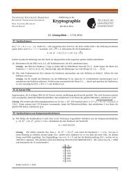
parameter w parameter v complexity evaluation complexity incl. precomp. #precomp. points 4 1 64A + 63D 71A+255D 15 4 2 64A + 31D 78A+255D 30 5 1 51A + 50D 66A+255D 31 5 2 51A + 25D 81A+255D 62 Table 4: Fixed point multiplication with off-line precomputation according to Lim and Lee in terms of expected point additions (A) and doublings (D). The parameters w and v are chosen to obtain a good trade off between total complexity and complexity in the evaluation phase for 256-bit curves. algorithm complexity formula #precomp. 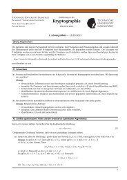points left-to-right binary Windowing (2 w + Windowing NAF ( 2w+1 3 λ(e) 2 A λ(e) � � λ(e) w − 3)A + � � λ(e)+1 w − 2)A Lim-Lee precomp: v(2 w−1 −1)A+(λ(e)− λ(e) wv )D main: λ(e) λ(e) w A + ( wv − 1)D � � λ(e) w � � λ(e)+1 w (2 w − 1) · v Table 5: Complexity evaluation formulas of algorithms with off-line precomputation [12, 13] same length and to process them parallelly as different exponents comparable to multiple point multiplication with shorter exponents. An additional parameter v specifies how the different exponents are further partitioned and can also be seen as the number of lookup tables containing the precomputed points [12]. In cases with no off-line precomputation the method by Lim and Lee can nearly compete with the window NAF methods. In cases with off-line precomputation the method by Lim and Lee performs significantly better than the window NAF methods. 3.2 Review of Basic Elliptic Curve Multiple Point Multiplication Techniques There are several methods available [12] which evaluate product sums k ·P +l·Q much more efficient than carrying out the individual multiplications sequentially and add the results. The complexity and the number of stored points for different approaches can be seen in Table 6. The respective complexity formulas are given in Table 7. While in the first three algorithms addition and doubling operations are done simultaneously, interleaving only does the doubling simultaneously. In our case the latter has some advantages. Firstly, the precomputed points rely on the points P and Q only. This allows storing precomputed points for further use. Secondly, the method allows for exponents with different lengths. Both is useful in our PACE scenario. algorithm parameter choices complexity #precomp. points Simultaneous mult. point w = 2 128A + 256D 15 Simultaneous slid. 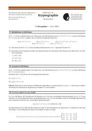window w = 2 118A + 256D 12 Simultaneous Joint Sparse Form (JSF) w-NAF Interleaving λ(e1) = λ(e2) = 256 w-NAF Interleaving λ(e1) = 256, λ(e2) = 128 − 129A + 255D 3 w1 = w2 = 5 99A + 258D 16 w1 = w2 = 5 78A + 258D 16 Table 6: Multiple point multiplication in terms of expected point additions (A) and doublings (D). The window parameters w are chosen to be optimal for 256-bit curves. algorithm complexity formula stored points Simultaneous mult. point (3·2 2(w−1) −2 w−1 −1+ 2 2w−1 2 2w � λ(e) w � − 1)A + (2 2(w−1) − 2 w−1 � � + λ(e) ( w − 1)w)D Simultaneous slid. window (3·2 2(w−1) −2 w−1 −1+ λ(e) w+1/3 )A + (22(w−1) − 2 w−1 � � λ(e) +( w −1)w)D Simultaneous (JSF) (1+ λ(e) 2 )A+(λ(e)−1)D 3 w-NAF Interleaving ( � j (2wj −2 − 1) + � λ(ej ) j wj +1 )A + (|j : wj > 2| + maxjλ(ej))D 2 2w − 1 2 2w − 2 2(w−1) � j (2w j −2 ) Table 7: Complexity evaluation formulas of multiple point multiplication algorithms [12] 4. OPTIMIZED PACE In this section we discuss the most promising optimizations for a PACE implementation on cell phones. The stated amounts of ADD and DBL are derived from the findings from Section 3 and express the average case. The proposed optimizations all lead to very similar theoretic execution times. Which one is the best in practice seems to depend on the actual hardware and the respective environmental circumstances. As we have seen in Section 3, storage space for points is not an issue on modern mobile devices, and is therefore not considered here. Likewise the time to load these points can be assumed to be negligible. Following the PACE specification (cf. Figure 1) the PCD conducts the EC computations shown in Equations (1) to (5). Counting the PCD’s EC computations in this notation leads to a total of 1 ADD and 5 MULT. X = x · G (1) H = x · Y (2) G ′ = s · G + H (3) �P KPCD = � SKPCD · G ′ (4) K = � SKPCD · � P KPICC (5)
4.1 Rearranging Equations When rearranging the equations we have to regard the following facts: X must be sent to the PICC in order to receive Y , and therefore it must be computed before H, G ′ , � P KPCD and K. � P KPCD must be sent to the PICC in order to receive � P KPICC and therefore it must be computed before K. In addition to Equation (3), G ′ is needed in the last PACE step (j), because it is part of the input for the computation of TP CD. Thus, G ′ should be a result or be computable from the result without increasing the overall computational cost. We consider the following possibilities for merging the equations. α: Standard Interleaving. One possible optimization is to merge Equations (2) and (3) as shown in Equation (6) to compute G ′ using interleaved multiplication. X, � P KPCD, and K are computed as shown in Equations (1), (4), and (5). This leads to an overall computation cost of 3 MULT and 1 PSUM. Using the best available algorithm and parameters, w-NAF Interleaving with w = 5, PSUM needs 78 ADD and 258 DBL (cf. Table 6). This is a vast improvement compared to 2 MULT evaluated as sequential single point w-NAF multiplications, which sum up to 78 ADD and 386 DBL (according to Table 2). A possible shortcoming is that s, which is only half the length of x, is forced into a scalar multiplication of the dimension of the size of x. G ′ = s · G + x · Y (6) β: Short Scalar Interleaving. The shortcoming of the above Equation (6) regarding the interleaved multiplication with s and x may be countered using the following trick: We know that the size of s is half the size of x. We break the pair (x, Y ) into two pairs (x1, Y1) and (x2, Y2) as is done when using the Lim-Lee method. The scalars x1, x2, and s now have the same size and the pair (s, G) can be added as third summand to the pairs (x1, Y1) and (x2, Y2) resulting in a standard interleaved multiplication with three summands as shown in Equation (7). As with Equation (6), X, � P KPCD, and K are computed as shown in Equations (1), (4), and (5). This leads to an overall computation cost of 3 MULT and 1 PSUM where the scalars in the PSUM are half the size of those of the PSUM of Equation (6). Using w-NAF Interleaving with w = 5 PSUM needs 85 ADD and 131 DBL according to Table 7 and additionally 128 DBL to prepare Y2. In total this is nearly the same as the PSUM costs resulting from Equation (6) and thus, is also a vast improvement compared to the not optimized version. G ′ = s · G + x1 · Y1 + x2 · Y2 (7) γ: Inversion. A third possibility is to merge Equations (2), (3), and (4) as shown in Equation (8) to compute � P KPCD using interleaved multiplication. G ′ then has to be computed by a scalar multiplication with an inverse as shown in Equation (9). X and K are computed as shown in Equations (1) and (5). This also leads to an overall computation cost of 3 MULT and 1 PSUM. w-NAF Interleaving leads to a cost of 99 ADD and 258 DBL (see Table 6). The necessary inversion and multiplications of scalars modulo the order r of the elliptic curve are neglectable in comparison to the operations on the points. A possible shortcoming is that the optimization potential of having an s of half the size of all other involved scalars is given away by multiplying it with a full size scalar. A possible advantage of this approach is that the computation of G ′ , which is not needed again until the last step of PACE is reached, can be delayed until then. �P KPCD = ( � SKPCD · s) · G + ( � SKPCD · x) · Y (8) G ′ = ( � SK −1 PCD mod r) · � P KPCD δ: Splitted Inversion. An also promising possibility to calculate � P KPCD is to reuse the precalculated points of G (see also Section 4.3) and evaluate Equation (10) with the Lim-Lee method. Another advantage of this method is the possibility to start the calculation of Equation (10) right after evaluating the first equation of the PACE algorithm (cf. Figure 1). Assumed the precomputed points or Lim-Lee multiplication are available, the evaluation of Equation (10) leads to 51 ADD and 25 DBL (cf. Table 4). The evaluation of Equation (11) results to 50 Add and 257 DBL (cf. Table 1). In total the Equations (10) to (12) that replace the PSUM in approach γ lead to 102 ADD and 282 DBL. (9) �P K1 = ( � SKPCD · s) · G (10) �P K2 = ( � SKPCD · x) · Y (11) �P KPCD = � P K1 + � P K2 (12) G ′ = ( � SK −1 PCD mod r) · � P KPCD (13) 4.2 Tweaked Implementation As seen above significant improvements are possible by applying well chosen multiplication algorithms and by rearranging the equations to be solved. However, there are possibilities for improvement concerning the implementation itself. In the following we consider possibilities to speed up the protocol execution taking into account at which points dedicated results have to be available and by avoiding overhead due to implementation techniques. Note that the optimizations are presented in a Java ME specific way, but can be applied to other languages analogously. Reorganization. Another possibility to speed up the calculations is the reorganization of their order. We present two different kinds of reorganizations. One possibility is to put some calculations at the beginning of the protocol before the initial contact with the eID card. To do so we need the domain-parameters of the used eID card saved on our device. These parameters can be stored at the first contact and can be used henceforward. The generation of the private keys x and �SKPCD as well as the computation of the first ephemeral key X (Equation (1)) could be done before actually starting the protocol. Additionally multiples of the base-point G could be stored in the NVM and later reused within the point multiplications. However, this is currently not supported by the existing Java ME-libraries. Another kind of reorganization regards the scheduling of the tasks and calculations during the protocol. Using threads for communication with the eID card allows us to use the time waiting for an answer from the card or the user for further calculations. The decryption of s can be threaded for instance, since the result will be required later in step (e) (cf. Figure 1).
Page 1 and 2: ABSTRACT An efficient mobile PACE i
Page 3: algorithm parameter choices complex
Page 7 and 8: Function / Provider FlexiProvider [
Page 9 and 10: nario which is in the scope of this

An efficient mobile PACE implementation - CDC

Create successful ePaper yourself

Delete template?

Save as template?