DesignCon 2002

More documents

Recommendations

Info

imperfections in the channel. The difference between those two waveforms is a “cursor”, as shown in Figure 4. Now, let us explore how we might calculate the inter-symbol interference (ISI) statistically. Let us assume that the current bit is a 1. This can happen in two different ways: either the previous bit was a 1, in which case there was no transition between them, or the previous bit was a 0, in which case there was a low-to-high transition between them. The probability of a transition is 0.5, if the bits are independent. In the first case, the cursor is zero; in the second case, it has some significant negative value, corresponding to the slow rise time of the step response at the end of the channel. Statistically, therefore, the waveform has a 50% chance of having no deviation, and a 50% chance of a negative deviation, equal to the cursor value. It is clear that we can chain this process forwards and backwards, considering each “postcursor” and precursor in turn. The primary difficulty is that, even if the bits are independent, the transitions are not; a high-to-low transition cannot be followed by another high-to-low transition; there must be a low-to-high transition in between. However, this constraint can be handled by the appropriate application of conditional probabilities. What comes out of all of the above considerations are probability distribution functions (PDFs) for the voltage value of the waveforms of high and low bits. These functions can be combined into cumulative distribution functions (CDFs), contours of which give the traditional eye diagram. 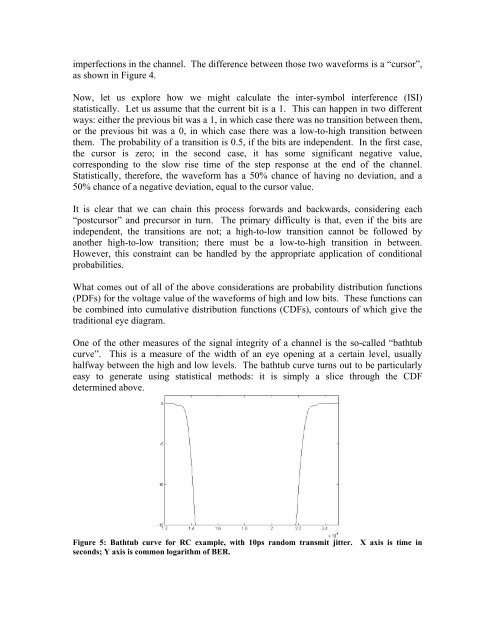One of the other measures of the signal integrity of a channel is the so-called “bathtub curve”. This is a measure of the width of an eye opening at a certain level, usually halfway between the high and low levels. The bathtub curve turns out to be particularly easy to generate using statistical methods: it is simply a slice through the CDF determined above. Figure 5: Bathtub curve for RC example, with 10ps random transmit jitter. X axis is time in seconds; Y axis is common logarithm of BER.
One of the great advantages of the statistical technique is that we can easily include the effects of random transmit jitter (standard deviation and not p-p), without resorting to Monte Carlo methods. This is done by applying the Gaussian probability distribution function to the time-location of each cursor, so that the cursors are not just impulses in voltage, but are spread out due to the Gaussian distribution in time, as shown in Figure 6: Figure 6: How random transmit jitter smears out the PDFs for the voltage cursors. One of the advantages of VerifEye over the public-domain tool called StatEye [5] is that VerifEye uses edges as its basis for calculations, rather than the pulses of StatEye. In part, this approach is made possible due to the high-quality transient responses that Nexxim provides for S-parameter-based circuits. The advantages of edge-based, rather than pulse-based, statistical eye calculations are primarily in two areas. First, by separating the rising and falling edges of the pulse, we can ensure that random jitter is indeed truly random: the timing of the edges can be statistically independent. And also, we can include the effects of duty cycle distortion (DCD), which can cause the width of pulse to vary. Pattern-based Analysis – QuickEye QuickEye uses some simplifying assumptions to create an eye diagram from transient simulation of a known sequence of single transitions.
Page 1 and 2: DesignCon 2008 BladeServer 10 Gb/s
Page 3 and 4: years. He worked at companies inclu
Page 5 and 6: eceiver has been implemented to sho
Page 7 and 8: Figure 1: Channel model topology Ea
Page 9 and 10: of high-speed design characteristic
Page 11: transitions due to jitter, it is po
Page 15 and 16: Figure 8: The response of a given c
Page 17 and 18: analysis enables rapid design chang
Page 19 and 20: acceptable BER. The native equaliza
Page 21 and 22: A B Figure 17: A: SIwave isometric
Page 23 and 24: Figure 20: BladeServer frequency do

DesignCon 2002

You also want an ePaper? Increase the reach of your titles

Delete template?

Save as template?