Neutron Scattering - JUWEL - Forschungszentrum Jülich

Member of the Helmholtz Association 

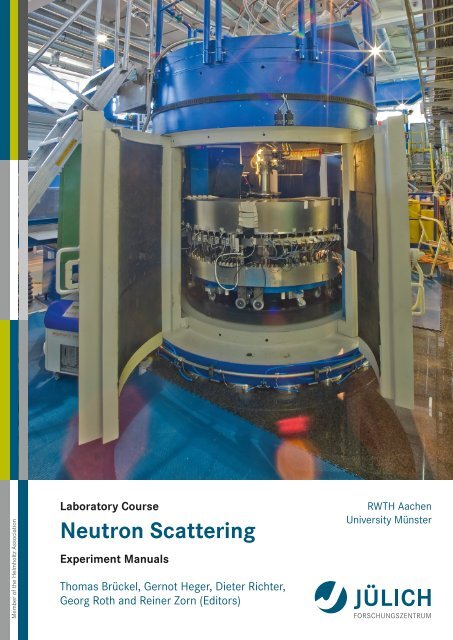
Laboratory Course 

Neutron Scattering 

Experiment Manuals 

Thomas Brückel, Gernot Heger, Dieter Richter, 

Georg Roth and Reiner Zorn (Editors) 

RWTH Aachen 

University Münster

Schriften des Forschungszentrums Jülich 

Reihe Schlüsseltechnologien / Key Technologies Band / Volume 40

Forschungszentrum Jülich GmbH 

Jülich Centre For Neutron Science (JCNS) 

Thomas Brückel, Gernot Heger, Dieter Richter, 

Georg Roth and Reiner Zorn (Editors) 

Neutron Scattering 

Experiment Manuals of the JCNS Laborator Course held at 

Forschungszentrum Jülich and the research reactor 

FRM II of TU Munich 

In cooperation with 

RWTH Aachen and University of Münster 


Reihe Schlüsseltechnologien / Key Technologies Band / Volume 40 

ISSN 1866-1807 ISBN 978-3-89336-790-0

Bibliographic information published by the Deutsche Nationalbibliothek. 

The Deutsche Nationalbibliothek lists this publication in the Deutsche 

Nationalbibliografie; detailed bibliographic data are available in the 

Internet at http://dnb.d-nb.de. 

Publisher and Forschungszentrum Jülich GmbH 

Distributor: Zentralbibliothek 

52425 Jülich 

Phone +49 (0) 24 61 61-53 68 · Fax +49 (0) 24 61 61-61 03 

e-mail: zb-publikation@fz-juelich.de 

Internet: http://www.fz-juelich.de/zb 

Cover Design: Grafische Medien, Forschungszentrum Jülich GmbH 

Printer: Grafische Medien, Forschungszentrum Jülich GmbH 

Copyright: Forschungszentrum Jülich 2012 


Reihe Schlüsseltechnologien / Key Technologies Band / Volume 40 

ISSN 1866-1807 

ISBN 978-3-89336-790-0 

The complete volume ist freely available on the Internet on the Jülicher Open Access Server (JUWEL) at 

http://www.fz-juelich.de/zb/juwel 

Neither this book nor any part of it may be reproduced or transmitted in any form or by any 

means, electronic or mechanical, including photocopying, microfilming, and recording, or by any 

information storage and retrieval system, without permission in writing from the publisher.

�� 

1 PUMA – Thermal Triple Axis Spectrometer O. Sobolev, A. Teichert, 

N. Jünke 

2 SPODI – High-resolution powder diffractometer M. Hoelzel, A. Senyshyn 

3 HEiDi – Hot Single Crystal Diffractometer for 

Structure Analysis with Neutrons 

M. Meven 

4 SPHERES – Backscattering spectrometer J. Wuttke 

5 DNS – Neutron Polarization Analysis Y. Su 

6 J-NSE – Neutron spin echo spectrometer O. Holderer, M. Zamponi, 

M. Monkenbusch 

7 KWS-1/-2 – Small Angle Neutron Scattering H. Frielinghaus, 

M.-S. Appavou 

8 KWS-3 – Very Small Angle Neutron Scattering 

Diffractometer with Focusing Mirror 

V. Pipich 

9 RESEDA – Resonance Spin Echo Spectrometer W. Häußler 

10 TREFF – Reflectometer S. Mattauch, U. Rücker 

11 TOFTOF – Time-of-flight spectrometer S. Busch, H. Morhenn, 

G. G. Simeoni, 

W. Lohstroh, T. Unruh

________________________ 

PUMA 

Thermal Triple Axis Spectrometer 

O. Sobolev, A. Teichert, N. Jünke 

Forschungsneutronenquelle Heinz Maier-Leibnitz (FRM II) 

Technische Universität München 

Manual of the JCNS Laboratory Course Neutron Scattering

2 O. Sobolev, A. Teichert, N. Jünke 

Contents 

1 Introduction .................................................................................................... 3 

2 Elastic scattering and Structure of Crystals ............................................... 4 

3 Inelastic Neutron Scattering and Phonons .................................................. 5 

4 Triple Axis Spectrometer PUMA ................................................................. 7 

5 Experiment Procedure .................................................................................. 9 

6 Preparatory Exercises ................................................................................. 12 

7 Experiment-Related Exercises ................................................................... 12 

Useful formula and conversions ....................................................................... 12 

References .......................................................................................................... 13 

Contact ............................................................................................................... 14

PUMA 3 

1. Introduction 

Excitations in crystals can be described using formalism of dispersion relations of the 

normal modes or quasi-particles (phonons, magnons, etc.). These relations contain the most 

detailed information on the intermolecular interactions in solids. 

The result of a neutron scattering experiment is the distribution of neutrons that have 

undergone an energy exchange �� = Ei - Ef, and a wave vector transfer, Q = ki – kf , after 

scattering by the sample.: 

d � 

� 

( 2 , ) � � ( , ) � ( , ) � 

d�d 

� 4 

4 � 

2 

� 

k f � coh 

� inc 

� � N Scoh 

Q � Sinc 

Q � 

(1) 

� 

k � 

� 

i 

�coh is coherent scattering cross section, �inc is incoherent scattering cross section. They are 

constants that can be found in tables (http://www.ncnr.nist.gov/resources/n-lengths/). S(Q,�) 

functions depend only on the structure and dynamics of the sample and do not depend on the 

interaction between neutrons and the sample. Sinc(Q,�) reflects individual motions of atoms. 

Scoh(Q,�) provides the information on the structure and collective excitations in the sample. 

Energy transfer 

�� = Ei - Ef 

Momentum transfer 

k k Q � � 

The triple axis spectrometer is designed for measuring the Scoh(Q,�) in monocrystals. 

Therefore this function is of special interest for us. 

k � 

0 

2mE 

� 

f 

� 

2� 

� 

2 2 

Q � k � k � 2k 

k 

i 

If ki = kf 

4� 

Q 

� 2ki sin� 

� sin� 

� 

f 

i 

f 

cos 2�


2. Elastic scattering and Structure of Crystals 

In the case of coherent elastic scattering, when � = 0 (ki = kf ) only neutrons, that 

fulfill the Brags law are scattered by the sample: 

n� = 2dhklsin�hkl, (2) 

where � is a wavelength of neutron, dhkl is a distance between crystal planes described by 

corresponding Miller indexes hkl. �hkl denotes the angle between incoming (outgoing) scattering 

beam and the (hkl) plane. 

For the analysis of the scattering processes in crystals it is convenient to use the concept of the 

reciprocal space. For an infinite three dimensional lattice, defined by its primitive vectors a1, 

a2 and a3, its reciprocal lattice can be determined by generating three reciprocal primitive 

vectors, through the formulae: 

a2 

� a3 

g1 

� 2� 

a � a � a 

g 

g 

2 

3 

1 

a1 

� a3 

� 2� 

a � a � a 

2 

a1 

� a2 

� 2� 

a � a � a 

3 

2 

1 

1 

3 

3 

2 

Note the denominator is the scalar triple product. Geometrically, the scalar triple product 

a1(a2�a3) is the volume of the parallelepiped defined by the three vectors. 

Let us imagine the lattice of points given by the vectors g1, g2 and g3 such that � is an 

arbitrary linear combination of these vectors: 

� � hg � kg 

� lg 

, (4) 

1 

2 

3 

where h,k,l are integers. Every point of the reciprocal lattice, characterized by � corresponds 

in the position space to the equidistant set of planes with Miller indices (h,k,l) perpendicular 

to the vector �. These planes are separated by the distance 

2� 

d hkl � (6) 

� hkl 

The Brag’s condition for diffraction can be expressed in the following vector form: 

Q = �hkl (7) 

A useful construction for work with wave vectors in reciprocal space is the Brillouin 

zone (BZ). The BZ is the smallest unit in reciprocal space over which physical quantities such 

as phonon or electron dispersions repeat themselves. It is constructed by drawing vectors from 

one reciprocal lattice points to another and then constructing lines perpendicular to these 

vectors at the midpoints. The smallest enclosed volume is the BZ. 

(3)

PUMA 5 

Fig.1 Real (left) and reciprocal (right) two dimensional lattices and BZ (gray area) 

3. Inelastic Neutron Scattering and Phonons 

Fig.2 Phonon dispersion curves for Ge. 

Atomic vibrations in a crystal can be analyzed in terms of lattice waves which are the 

normal modes of the crystal. The frequencies of normal modes � are related to their wave 

vectors q (q = 2�/�) by the dispersion relations 

� = �j(q), (7) 

where the index j denotes a particular branch. For a crystal with N atoms per primitive unit 

cell there are 3N branches of the frequency spectrum. Three branches are acoustic ones for 

which � � 0 as q � 0; the other 3N-3 are branches are optical branches for which � tends to 

a finite value as q � 0. In certain directions of high symmetry the normal vibrations are 

strictly transverse or longitudinal. The energy quantum �� is called phonon in analogy to the 

phonon for electromagnetic waves.


If we want to measure the frequency of a phonon � for a certain q, the basic scattering 

conditions must fulfil the energy and momentum conservation laws: 

� 2 2 

E i � E f � ( ki 

� k f ) � ��( 

q) 

(9) 

2mn 

Q = ki – kf = G � q 

When the above conditions are fulfilled, the function Scoh(Q,�) shows a peak. We can held Q 

constant and vary ki (kf) to measure intensity of scattered neutrons at different energy 

transfers. In order to keep Q, and thus q, constant while varying ki, the scattering angle must 

change as well as the relative orientation of the crystal with respect to kf. 

The intensity of neutrons scattered by phonon is proportional to the square of the 

dynamical structure factor F(Q): 

�q� 2 Q �e 

� j 

2 

coh ( Q, �) ~ F( 

Q) 

�b� 

exp��W�exp( 

�iqr� 

) , (10) 

m 

S � k 

� 

� 

Where sum is taken over all atoms in unit cell with coordinates rk , exp(-W) is a Debye- 

Waller factor, ek denotes the polarization vector of the phonon. The scalar product Q � e� 

�q j � 

means that only lattice vibrations polarized along the momentum transfer are visible. This 

makes possible to distinguish transverse (TA) and longitudinal (LA) acoustic modes. For TA 

modes e�q, and therefore Q must be perpendicular to q, while for a LA mode, one must take 

Q�� q (Fig. 3) 

Fig. 3 Top: LA and TA phonons. Bottom: Neutron scattering diagram in the reciprocal space 

for TA (left ) and LA phonons

PUMA 7 

4. Triple Axis Spectrometer PUMA 

The three-axis instrument is the most versatile instrument for use in inelastic scattering 

because it allows one to probe nearly any coordinates in energy and momentum space in a 

precisely controlled manner. The three axes correspond to the axes of rotation of the 

monochromator (axis1), the sample (axis2), and the analyzer (axis3). The monochromator 

crystal selects neutrons with a certain energy from the white neutron beam emanating from 

the reactor. The monochromatic beam is then scattered off from the sample (second axis). The 

neutrons scattered by the sample can have a different energy from those incident on the 

sample. The energy of these scattered neutrons is then determined by the analyzer crystal 

(third axis). All three angles (�M, �S, �A) can vary during an experiment, the sample table and 

analyzer are equipped with air pads, so that they can glide over the “Tanzboden” (dancing 

floor). Below, we describe in detail each component of a triple-axis spectrometer. 

Monochromator 

A crystal monochromator is used to select neutrons with a specific wavelength. Neutrons with 

this wavelength interact with the sample and are scattered off at a similar (elastic) or different 

wavelength (inelastic). The energy of the neutrons both incident on and scattered from the 

sample is determined by Bragg reflection from the monochromator and analyzer crystals, 

respectively. For a specific Bragg plane (hkl) characterized by an interplanar spacing dhkl, the 

crystal is rotated about a vertical axis. A pyrolytic graphite with d002 = 3.35 Å (PG(002)) and 

a copper with d220 = 1.28 Å (Cu(220)) monochromators are available at PUMA. The angular 

range of the monochromator 2�M is of 15 o - 115°. The PG(002) is usually used for energies 

below 50meV (�>1.3Å). For higher incident energies the Cu(220) can be used. 

Sample table 

The sample table from the company Huber provides a possibility to vary independently both 

2�s and �S. It is equipped with a goniometer moving the sample in the three translation axes x, 

y and z and tilting. The tilt angle is ±15°. Single crystal experiments can be performed with an 

Euler cradle at PUMA. The sample environment includes magnets, pressure cells, cryostats 

and high temperature furnace. 

Analyzer 

Like the monochromator, the PG(002) analyzer consist of 20x5 separate analyzer crystal 

plates are mounted in an aluminum frame. There is an option to measure with the flat or 

horisontaly and verticaly focused analyser. The angular range of the analysator 2�M is of 

-130 o - 130°. 

Detector and monitor 

The detector consists of five counter tubes which are filled with a 3 He pressure of 5 bar. To be 

able to monitor the neutron flux incident on the sample, a low-efficiency neutron counter 

monitor is usually placed before the sample. Such a monitor is required so that flux variation 

caused by, for example, the reactor power fluctuations and the change in reflectivity of the 

monochromator with neutron wavelength can be automatically corrected for.


Fig.4 PUMA spectrometer. 

Slits, Collimators, Filter 

Additional components like slits or collimators are used to define the beam cross 

section. Collimators (�1- �4) are used for the improvement of the resolution and to specify 

the beam divergence. They consist of multiple parallel arranged Gd2O3 coated foils with a 

defined angle to the beam. The angular divergence of the collimator in the horizontal plane � 

is defined by the distance between foils �d and the length of the collimator l (tan � = �d / l). 

Different collimators with a horizontal divergence between 10’ and 60’ are available at the 

instrument. 

One of the problems of the TAS method is the possible presence of higher harmonics 

in the neutron beam. Higher harmonics arise from higher order (hkl) in Bragg’s law (2). This 

means that if the monochromator (analyzer) crystal is set to reflect neutrons with a 

wavelength of � from a given (hkl) plane, it will also reflect neutrons with wavelength �/n. 

This leads to the appearance of several types of spurious peaks in the observed signal. 

Different filters are used to eliminate the high-order neutrons and to reduce the background. 

There are a sapphire filter (Al2O3) and an erbium filter (Er) at PUMA. They are installed in 

front of the monochromator. Sapphire filter is used wavelengths ��> 1 Å and reduce the 

background inducing by the epithermal neutrons. Erbium filter is suitable as �/2 filter for � 

between 0.5 and 1Å as well as �/3 filter for � between 0.7 and 1.6Å.

PUMA 9 

Components 

Axis PUMAs 

notation 

Description 

Monochromator M �M mth Monochromator Theta 

2�M mtt Monochromator 2Theta 

mtx, mty Monochromator Translation x-, y- direction 

mgx, mgy Monochromator Goniometer x-, y- direction 

mfh, mfv Monochromator Focus horizontal, vertical 

Sample S �S psi Sample Theta 

2�S phi Sample 2Theta 

stx, sty, stz Sample Translation x-, y-, z- direction 

sgx, sgy Sample Goniometer x-, y- direction 

Analyzer A �A ath Analyzer Theta 

2�A att Analyzer 2Theta 

atx, aty Analyzer Translation x-, y- direction 

agx, agy Analyzer Goniometer x-, y- direction 

afh Analyzer Focus horizontal 

Collimators alpha1 – alpha4 Collimation 

5. Experiment Procedure 

The aim of the experiment is to measure acoustic phonons in a germanium sample. The 

phonons will be measured for [110] (LA) and [001] (TA) directions in [220] BZ. 

The experimental procedure shall contain the following steps: 

Sample alignment 

It is very difficult to align a sample with triple axis spectrometer, if the sample orientation is 

absolutely unknown. A sample must be pre-aligned, this means that the vertical axis of the 

sample must be known and roughly perpendicular to the ‘Tanzboden’. Than we shall do the 

following steps: 

- Inform the control program of the spectrometer about a scattering plane of the sample. One 

must set two reciprocal vectors (in our case [110] and [001]) laying in the scattering plane. 

- Drive spectrometer (�M, 2�M, �S, 2�S, �A, 2�A,) to the position corresponding to [220] 

reflection. 

- Scan �S and find the Brag’s peak. 

- Scan corresponding goniometer axes to maximize intensity of the peak. 

- Do the same for other reflection [004]. 

- Change the offset of the �S so that the nominal �S values correspond to intensity maxima for 

the above reflections. 

Phonons measurements 

For our measurements we will chose the const-kf configuration with kf = 2.662 Å -1 (Ef = 14.68 

meV). This means that we will scan the energy transfer �� = Ei – Ef by varying incident 

energy Ei (ki). We are going to use PG(002) monochromator.


For LA phonon we will do constant-Q scans in the energy transfer range �� = 0 – 21 meV (0 

– 8 THz) for the following points: 

Q(r.l.u.) = (2.1, 2.1, 0), (2.2, 2.2, 0), (2.3, 2.3, 0), (2.4, 2.4, 0), (2.5, 2.5, 0), (2.6, 2.6, 0), (2.7, 

2.7, 0), (2.75, 2.75, 0). 

For TA phonon we will do constant-Q scans in the energy transfer range �� = 0 – 15 meV (0 

– 3.6 THz) for the following points: 

Q(r.l.u.) = (2, 2, 0.2), (2, 2, 0.3), (2, 2, 0.4), (2, 2, 0.5), (2, 2, 0.7), (2, 2, 0.8), (2, 2, 0.9), (2, 2, 

1).

PUMA 11 

a) PG Analyzer b) Soller collimator 

c) Sample table d) Shutter, filters and collimators 

e) Analyzer and Detector f) Detector, consists of 5 3 He tubes 

Fig 5 Elements of PUMA


6. Preparatory Exercises 

1. Calculate angles �M, 2�M, �S, 2�S for the reflections [220] and [004] of germanium (cubicdiamond, 

a = 5.66 Å), supposing that kf = 2.662 Å -1 = const, monochromator is PG(002), and 

check, if this reflections are measurable with our experimental setup. 

2. Before doing a scan it is important to check that all point in Q - �� space are available, 

instrument angles do not exceed high or low limits. Also, an experimental scientist must be 

sure that the moving instrument will not hit walls or any equipment. Calculate instrument 

parameters (�M, 2�M, �S, 2�S) for the momentum transfers Q (r.l.u.) = (2.1, 2.1, 0), (2.75, 

2.75, 0) and energy transfers �� = 0 and 21 meV. This can be done using an online triple-axis 

simulator: 

http://www.ill.eu/instruments-support/computing-for-science/cs-software/all-software/vtas/ 

7. Experiment-Related Exercises 

1. Plot obtained spectra for each Q as a function of energy (THz). Fit the spectra with 

Gaussian function and find centers of the phopon peaks. The obtained phonon 

energies plot as a function of q. 

2. Why triple-axis spectrometer is the best instrument to study excitations in single 

crystals? 

3. During this practicum we do not consider some problems that are very important for 

planning experiments with a triple axis instrument such as resolution and intensity 

zones [2]. Persons who have a strong interest to the triple-axis spectroscopy should 

study these topics by oneself. Advanced students should be able to explain our choice 

of Brillouin zone and parameters of scans for the phonon measurements. 

Useful formula and conversions 

1 THz = 4.1.4 meV 

n� = 2dhklsin�hkl, 

2� 

d hkl � 

� 

0 

hkl 

Q � k � k 

2 2 

Q � k � k � 2k 

k 

i 

f 

f 

i 

f 

cos 2� 

4� 

If ki = kf (elastic scattering) Q � 2ki sin� 

� sin� 

� 

E [meV] = 2.072 k 2 [Å -1 ]

PUMA 13 

References 

[1] Ch. Kittel, Einführung in die Festkörperphysik, Oldenburg, 14th ed., 2006 

[2] G. Shirane, S.M. Shapiro, J.M. Tranquada, Neutron Scattering with a Triple-Axis 

Spektrometer, Cambridge University Press, 2002 

[4] G. Eckold, P. Link, J. Neuhaus, Physica B, 276-278 (2000) 122- 123 

[5] B.N.Brockhouse and P.K. Iyengar, Physikal Review 111 (1958) 747-754 

[6] http://www.ill.eu/instruments-support/computing-for-science/cs-software/allsoftware/vtas/


Contact 

PUMA 

Phone: + 49 89 289 14914 

Web: http://www.frm2.tum.de/wissenschaftliche-nutzung/spektrometrie/puma/index.html 

Oleg Sobolev 

Georg-August Universität Göttingen 

Institut für Physikalische Chemie 

Aussenstelle am FRM II 

Phone: + 49 89 289 14754 

Email: oleg.sobolev@frm2.tum.de 

Anke Teichert 

Georg-August Universität Göttingen 

Institut für Physikalische Chemie 

Aussenstelle am FRM II 

Phone: + 49 89 289 14756 

Email: anke.teichert@frm2.tum.de 

Norbert Jünke 

Forschungsneutronenquelle Heinz Maier-Leibnitz 

ZWE FRM II 

Phone: + 49 89 289 14761 

Email: norbert.juenke@frm2.tum.de

________________________ 

SPODI 

High-resolution powder diffractometer 

M. Hoelzel, A. Senyshyn 




2 POWDER DIFFRACTOMETER SPODI 

Contents 

1 Applications of neutron powder diffraction ................................................ 3 

2 Basics of Powder Diffraction ........................................................................ 4 

3 Information from powder diffraction experiments .................................. 11 

4 Evaluation of Powder Diffraction Data ..................................................... 13 

5 Comparison between Neutron and X-ray diffraction .............................. 15 

6 Setup of the high-resolution neutron powder diffractometer 

SPODI at FRM II ........................................................................................ 17 

7 Experiment: Phase- and structure analysis of lead titanate at various 

temperatures ................................................................................................ 20 

References .......................................................................................................... 23 

Contact ............................................................................................................... 24

POWDER DIFFRACTOMETER SPODI 3 

1. Applications of neutron powder diffraction 

Powder diffraction reveals information on the phase composition of a sample and the 

structural details of the phases. In particular, the positions of the atoms (crystallographic 

structure) and the ordering of magnetic moments (magnetic structure) can be obtained. In 

addition to the structural parameters, also some information on the microstructure (crystallite 

sizes/microstrains) can be obtained. The knowledge of the structure is crucial to understand 

structure – properties – relationships in any material. Thus, neutron powder diffraction can 

provide valuable information for the optimisation of modern materials. 

Typical applications: 

Material Task 

Lithium-ion battery materials Positions of Li atoms, structural changes/phase 

transitions at the electrodes during operation, 

diffusion pathways of Li atoms 

Hydrogen storage materials Positions of H atoms, phase transformations 

during hydrogen absorption/desorption 

Ionic conductors for fuel cells positions of O/N atoms, thermal displacement 

paramteters of the atoms and disorder at 

different temperatures, 

diffusion pathways of O/N atoms 

Shape memory alloys stress-induced phase transforamtions, stressinduced 

texture development 

materials with CMR effect magnetic moment per atom at different 

temperatures 

catalysers Structural changes during the uptake of sorbents 

Piezoelectric ceramics Structural changes during poling in electric field, 

positions of O atoms 

Nickel superalloys Phase transformations at high temperatures, 

lattice mismatch of phases 

magnetic shape memory alloys Magneto-elastic effects, magnetic moment per 

atom at different temperatures and magnetic 

fields


2. Basics of Powder Diffraction 

Diffraction can be regarded as detection of interference phenomena resulting from coherent 

elastic scattering of neutron waves from crystalline matter. Crystals can be imagined by a 

three-dimenional periodic arrangement of unit cells. The unit cell is characterised by the 

lattice parameters (dimensions and angles) and the positions of atoms or molecules. 

For diffraction experiments the probe should have a wavelength comparable to interatomic 

distances: this is possible for X-rays, electrons or neutrons. 

Structure factor 

The structure factor describes the intensity of Bragg reflections with Miller indexes (hkl), 

based on the particular atomic arrangement in the unit cell 

F 

hkl 

� 

n 

� 

j�1 

b T exp 

j 

j 

� � 

�2� iHR 

� 

j 

where 

Fhkl: structure factor of Bragg reflection with Miller indexes hkl. 

n: number of atoms in unit cell 

bj: scattering lengths (in case of neutron scattering) or atomic form factor (in case of X-ray 

diffraction) of atom j 

Tj: Debye Waller factor of atom j 

The scalar product H Rj consists of the reciprocal lattice vector H and the vector Rj, revealing 

the fractional atomic coordinates of atom j in the unit cell. 

�h 

� � x j � 

� � � � � � 

HR j � �k 

� �� 

y j � � hx j � ky j � lz j 

� l � � 

z 

� 

� � � j � 

Thus, the structure factor can also be given as follows: 

F 

hkl 

� 

n 

� 

j�1 

b T exp 

j 

j 

�hx � ky � lz � 

j 

j 

j 

The intensity of a Bragg reflection is proportional to the square of the absolute value of the 

2 

structure factor: I � Fhkl 

Debye-Waller Factor 

The Debye-Waller Factor describes the decrease in the intensity of Bragg reflections due to 

atomic thermal vibrations.


T ( Q) 

j 

� 1 

exp�� 

� 2 

� 

� �� 

Qu 

� j 

vector uj reflects the thermal displacements of atom j 

Braggs' Law 

Braggs' Law provides a relation between distances of lattice planes with Miller indexes hkl, 

i.e. dhkl, and the scattering angle 2� of the corresponding Bragg peak. Braggs' law can be 

illustrated in a simplified picture of diffraction as reflection of neutron waves at lattice planes 

(figure 4). The waves which are reflected from different lattice planes do interfere. We get 

constructive interference, if the path difference between the reflected waves corresponds to an 

integer multiple of the wavelength. 

The condition for constructive interference (= Braggs' law) is then: 

2 

d hkl 

sin� 

� n� 

Figure 1: Illustration of Bragg’s law: constructive interference of neutron waves, reflected 

from lattice planes, where �, 2� are Bragg angles, 2�=2dhklsin� is the path difference and 

2�=n� is the constructive interference. 

Applying Bragg’s law one can derive the lattice spacings (“d-values“) from the scattering 

angle positions of the Bragg peaks in a constant-wavelength diffraction experiment. With the 

help of d-values a qualitative phase analysis can be carried out.


Ewald's sphere 

The Ewald's sphere provides a visualisation of diffraction with help of the reciprocal lattice. 

At first, we introduce the scattering vector Q and the scattering triangle (Figure 2). The 

incident neutron wave is described by a propagation vector ki, the scattered wave is given by 

kf. In the case of elastic scattering (no energy transfer) both vectors ki and kf have the same 

length which is reciprocal to the wavelength. 

k 

i 

k 

� f 

2� 

� 

� 

remark: 

The length of the wave vectors are sometimes given as k i � k f 

1 

� (This definition is found 

� 

esp. in crystallographic literature, while the other one is more common for physists). 

The angle between vectors ki and kf is the scattering angle 2�. The scattering vector Q is the 

given by the difference between ki and kf : 

Q= k f � k i 

� 

� 

� 

sin 

Q � 4 

Figure 2: Illustration of scattering vector and scattering angle resulting from incident and 

scattered waves. 

In the visualisation of the diffraction phenomena by Ewald the scattering triangle is 

implemented into the reciprocal lattice of the sample crystal – at first, we consider diffraction 

at a single crystal (Figure 3). Note that the end of the incident wave vector coincides with the 

origin of the reciprocal lattice. Ewald revealed the following condition for diffraction: we 

have diffraction in the direction of kf, if its end point (equivalently: the end point of scattering 

vector Q) lies at a reciprocal lattice point hkl. All possible kf, which fulfil this condition, 

describe a sphere with radius ��, the so called Ewald's sphere. Thus we obtain a hkl 

reflection if the reciprocal lattice point hkl is on the surface of the Ewald's sphere.


Figure 3: Illustration of diffraction using the Ewald's sphere. 

2� 

Here, the radius of Ewald's sphere is given by 1/� (For ki � we obtain a radius of ��). 

� 

We receive the following condition for diffraction: the scattering vector Q should coincide 

with a reciprocal lattice vector Hhkl (x 2�): 

� � � 

Q � 2�H 

hkl ; H hkl 

� � 

x x � � 

x 

� ha 

� kb 

� lc 

; H hkl 

x 1 

� d hkl � 

d hkl 

From this diffraction condition based on the reciprocal lattice we can derive Bragg's law: 

� � sin� 

2� 

Q � 2� H hkl � 4� 

� � 2d 

hkl sin� 

� � 

� d 

hkl 

The Ewald's sphere is a very important tool to visualize the method of single crystal 

diffraction: At a random orientation of a single crystalline sample a few reciprocal lattice 

points might match the surface of Ewald's sphere, thus fulfil the condition for diffraction. If 

we rotate the crystal, we rotate the reciprocal lattice with respect to the Ewald's sphere. Thus 

by a stepwise rotation of the crystal we receive corresponding reflections.


Powder Diffraction in Debye-Scherrer Geometry 

In a polycrystalline sample or a powder sample we assume a random orientation of all 

crystallites. Correspondingly, we have a random orientation of the reciprocal lattices of the 

crystallites. The reciprocal lattice vectors for the same hkl, i.e. Hhkl, describe a sphere around 

the origin of the reciprocal lattice. In the picture of Ewald's sphere we observe diffraction 

effect, if the surface of the Ewald's sphere intersects with the spheres of Hhkl vectors. For a 

sufficient number of crystallites in the sample and a random distribution of grain orientations, 

the scattered wave vectors (kf) describe a cone with opening angle 2� with respect to the 

inident beam ki. 

In the so called Debye-Scherrer Geometry a monochromatic beam is scattered at a cylindrical 

sample. The scattered neutrons (or X-rays) are collected at a cylindrical detector in the 

scattering plane. The intersection between cones (scattered neutrons) and a cylinder (detector 

area) results in segments of rings (= Debye-Scherrer rings) on the detector. By integration of 

the data along the Debye-Scherrer rings one derives the conventional constant-wavelength 

powder diffraction pattern, i.e. intensity as a function of the scattering angle 2�. 

Relative intensity 

0 20 40 60 80 100 120 140 160 18 

Bragg angle, 2� (deg) 

Figure 4: Illustration of powder diffraction in Debye-Scherrer Geometry. On the left: cones of 

neutrons scattered from a polycrystalline sample are detected in the scattering plane. On the 

right: resulting powder diffraction pattern.


Figure 5: Two dimensional diffraction data (detector height vs. scattering angle 2�), collected 

at high-resolution powder diffractometer SPODI, illustrating the Debye-Scherrer rings of a 

corundum sample.


Relations between Bragg positions and lattice parameters 

With the help of Braggs law one can derive the lattice spacings “d-values” directly from the 

positions of Bragg reflections. The d-values are related with the lattice parameters of the unit 

cell (the cell dimensions a,b,c and the cell angles ��) and the Miller indexes (hkl) of the 

corresponding reflections. In the following, the relations are provided for the different crystal 

systems. 

2 2 

cubic 

d hkl 

� 2 

a 

1 

h 

4 h 

� k 

� l 

2 

2 2 

hexagonal 

d hkl 

� 

3 

2 

a 

� 2 

c 

1 

2 

� hk � k 

2 2 2 

tetragonal 

d hkl 

� 2 

a 

� 2 

c 

1 

h 

� k 

2 2 2 

orthorhombic 

d hkl 

� � � 

2 2 2 

a b c 

monoclinic 

1 

1 

d hkl 

h 

k 

l 

l 

l 

2 

2 

2 

h k l 2hl 

cos � 

� 

� � � 

2 2 2 2 2 

2 

a sin � b c sin � acsin 

�


3. Information from powder diffraction experiments 

neutron counts 

22000 

20000 

18000 

16000 

14000 

12000 

10000 

8000 

6000 

4000 

2000 

0 

-2000 

20 30 40 50 60 70 80 

2� [°] 

90 100 110 120 130 

Figure 6: on the left: typical powder diffraction pattern. On the right: zoom on a single Bragg 

peak. 

In the following, we will consider the information which can be derived from different 

elements of the diffraction patterns. 

Positions (scattering angles) of Bragg reflections 

� phase identification (from d-values) 

� lattice parameters 

� symmetry information (space group) by lattice parameters and selection rules (systematic 

extinction of reflections) 

Intensity of Bragg reflections 

experimental 

calculated 

Difference (exp - calc) 

Bragg positions 

� crystallographic structure 

� positions of atoms (fractional atomic coordinates) 

� occupancies of atoms on their sites 

� thermal displacement parameters 

� magnetic structure 

� magnetic lattice (propagation vector) 

� magnetic symmetry (space group) 

� magnetic moment per atom 

� quantitative phase analysis 

� preferred orientation effects 


25000 

20000 

15000 

10000 

5000 

intensity 

width 

background 

0 

40.5 41.0 

position 

41.5 

2� [°] 

42.0 42.5


Profiles of reflections 

The reflection profiles result in a convolution of the instrumental resolution function with 

broadening effects of the sample 

� microstructural information 

� microstrains 

� crystallite sizes 

Modulation/Profile of Background 

� short range order 

� disorder 

� amorphous contents


4. Evaluation of Powder Diffraction Data 

The methods of data treatment can be classified in analysis of phase composition or phase 

transformation, structure solution and structure refinement. 

Qualitative phase analysis is based on the determination of d-values and relative intensities (in 

particular intensities of strong reflections have to be considered). The phase identification is 

supported by crystallographic data bases (ICDD, ISCD), literature data and information from 

other methods (for instance, analysis of the chemical composition). Such kind of phase 

analysis is however typically carried out with X-ray diffraction. 

The majority of neutron powder diffraction studies is based on experiments at various 

temperatures to investigate phase transformation behaviour as a function of temperature. 

There is an increasing demand for parametric studies, i.e. diffraction studies under various 

environmental conditions (temperature, electric or magnetic field, mechanical stress, gas 

atmosphere...) with particular attention to reaction pathways/reaction kinetics. This kind of 

investigations require in general high-intensity powder diffraction. 

Powder diffracton data can be used either for phase identification or for the refinement of 

structural parameters, such as lattice parameters, fractional atomic coordinates, atomic 

occupancies and atomic displacement parameters by the full profile Rietveld analysis. In the 

Rietveld method, the full diffraction pattern is calculated by a structure model, taking into 

account the above mentioned structural parameters, as well as reflection profile parameters, 

instrumental parameters and background parameters. Using least-squares method, the 

experimental data can be fitted to the model in a stepwise refinement of the parameters. The 

complexity of the structures is directly dependent on the instrument specification, in 

particular, high-resolution powder diffractometers are designed for structure refinements on 

complex systems. 

Besides structure refinement, also structure solution can be done based on powder diffraction 

patterns by various methods.



60000 46 % Ti 

Iobs Icalc 50000 

difference plot 

Bragg positions 

40000 

30000 

20000 

10000 

-10000 

0 

20 30 40 50 60 70 80 90 100 110 120 130 140 150 160 

2� 


6000 

5000 

4000 

3000 

2000 

1000 

1/2 (311) c 

Cm 

0 

36 37 38 39 40 

Figure 7: Data treatment of a measurement on the ferroelectric Pb0.99La0.01Zr0.54Ti0.46O3, 

carried out at 5 K at diffractometer SPODI (FRM II): Diffraction pattern including 

experimental data, calculated data by Rietveld fit, Bragg reflection positions of the phases 

(space groups CC and Cm) and difference plot (between experimental and calculated data). - 

zoom into the diffraction pattern, hightlighting a superlattice reflection of the CC phase. - 

structure model of the CC phase, view in the [001]c direction - structure model of the CC 

phase, view in the [010]c direction. In particular, the superstructure in the tiltings of oxygen 

octahedra can be seen. 

2� 

(111) c 

Cc


5. Comparison between Neutron and X-ray diffraction 

I) X-rays are scattered at electrons, neutrons are scattered at nuclei 

In case of X-ray scattering, the scattering power of an atom (described by the atomic form 

factor f) is proportional to the number of electrons. 

Neutrons are scattered at nuclei. Thus the interaction (described by the scattering length b) 

varies between different isotopes of an element. Scattering length of neighbouring elements in 

the periodic system can be very different. 

implications: 

Localisation of light elements next to heavier ones 

X-ray diffraction is a powerful tool to determine the positions of heavy atoms, but the 

localisation of light atoms in the vicinity of much heavier atoms is often difficult or related 

with high uncertainties. Neutron diffraction is advantageous to localise light atoms such as H, 

D, Li, C, N, O. 

Localisation of neighbouring elements in the periodic table 

Neighbouring elements in the periodic table can hardly be distinguished by means of X-ray 

diffraction. Neutrons are advantageous for such cases: examples: Mn – Fe - Co – Ni or O – N. 

Q-dependence of intensities 

Since the size of electron clouds is comparable to the wavelength, the atomic form factor 

depends on sin��or�Q��Therefore the intensities of X-ray reflections decrease significantly 

for increasing Q (increasing scattering angles 2�� . 

As the range of the neutron–nuclei–interaction is by orders of magnitude smaller than the 

wavelengths of thermal neutrons, scattering lengths do not depend on Q. As a consequence, 

neutron diffraction patterns do not show a decrease of Bragg reflection intensities for higher 

scattering angles, enabling the analysis of larger Q-ranges. In particular, neutron diffraction is 

advantageous for the analysis of thermal displacement parameters. 

II) neutrons interact weakly with matter 

implications: 

sample volume


The flux from neutron sources much lower compared to X-ray tubes or even synchrotrons. In 

addition, neutrons interact weakly with matter. Therefore, much larger sample amounts are 

required compared to X-ray diffraction (“grams instead of milligrams”). On the other hand 

this weak interaction results in much higher penetration depths of neutrons, compared to 

laboratory X-ray diffractometers. Thus, polycrystalline bulk samples can be investigated. 

Furthermore, using large sample volumes avoids possible problems due to preferred 

orientation effects. In principle, bulk samples can also be investigated with high-energy 

synchrotron radiation. Anyhow in special cases the very low scattering angles related to low 

wavelength (in high-energy synchrotron studies) can cause difficulties. 

Sample environments 

The large penetration depths of neutrons facilitate the usage of sample environments like 

cryostat, furnaces, magnets... In general neutron scattering experiments are more powerful 

applying high or low temperatures. On the other hand, the small sample volume required for 

synchrotron studies gives better possibilities for high-pressure experiments. 

III) neutrons exhibit a magnetic moment 

Though neutrons do not have an electric charge, the internal charge distribution due to its 

three quarks along with the spin result in a magnetic moment of the neutron. 

implications: 

magnetic scattering 

The interaction between the magnetic moment of the neutron and a possible magnetic 

moment of an atom results in a magnetic scattering contribution, incidentally in the same 

order of magnitude as the nuclear scattering contribution. The magnetic scattering 

contribution can be easily detected by means of neutron diffraction. In synchrotron diffraction 

studies, possible magnetic scattering events are by several orders of magnitude weaker than 

the Thomson scattering.


6. Setup of the high-resolution neutron powder diffractometer SPODI at 

FRM II 

The main components of a constant-wavelength neutron powder diffractometer are: source, 

monochromator, sample and detector. Between these components collimation systems are 

installed which have high impact on the instrumental resolution function and the neutron flux. 

detector 

primary collimator 

monochromator 

angle: 2�M 

mosaicity: � 

�1 

detector collimator 

�3 

neutron guide 

secondary collimator 

�2 

sample 

thermal 

neutrons 

Figure 8: illustration of a typical instrumental layout, introducing the parameters used by 

Caglioti to describe the instrumental resolution function. 

Instrumental resolution function 

source 

As shown by Calgioti, the instrumental resolution function of a constant-wavelength powder 

diffractometer can be approximated by: 

FWHM � U tan � �V 

tan� 

�W 

2 

with the Caglioti parameters:


4 

U � 

tan 

V � 

tan 

� 

W � 

2 2 2 2 2 2 

��1�2��1��2�� 2 2 2 2 

�m 

��1��2�4�� 2 2 2 

� 4� 

2 ��1�2�� 2 2 2 

�m 

��1��2�4�� 2 2 2 2 2 2 2 2 2 

1� 

2 ��1 

�3 

�� 

2� 

3 � 4� 

��2��3� 2 2 2 

��4�� 1 

2 

in this approach it is assumed that all components have Gaussian transmission profiles. The 

resolution function is determined by the horizontal beam divergences �� the 

monochromator angle 2�m and the mosaicity of the monochromator �� (Figure 8). As the 

impact of these parameters on the instrumental resolution function can be estimated, the 

Caglioti equations help to design an instrument to achieve a designated performance. 

However, it should be emphasised that in the approximations of Caglioti only the horizontal 

beam divergences are taken into account, neglecting vertical beam divergences by a vertical 

focusing monochromator or a vertical divergent neutron guide. Those effects are taken into 

account by ray-tracing methods, which allow a detailed modelling of the individual 

components. 

The powder diffractometer SPODI has been designed to achieve both high resolution and 

good profile shape. In its standard configuration (highest resolution mode) SPODI uses a 

unique very high monochromator take-off angle of 155° along with a large monochromatorto-sample 

distance of 5 meters. An evacuated beam tube of about 4 m in length is located 

between the monochromator and the sample which also controls both vertical and horizontal 

neutron beam divergences at the sample position. Thus the natural neutron beam divergence 

in horizontal plane is 25’ only. It can be reduced down to even 5’ by optional Soller 

collimators in front of the sample. 

Monochromator 

At constant-wavelength diffractometers, the monochromatisation is perfomed using crystals 

followings Bragg's equation: 

2d hkl sin� 

� � , where the effective transmission band is determined by a derivative 

�� 

� �� 

M cot� 

M 

� 

The width of the wavelength band �� strongly depends on the monochromator angle 

2�m and the mosaicity of the monochromator ��m . Thus these parameters have a 

major impact on the instrumental resolution function and the flux on the sample.


Typically, the monochromator crystals are installed at a vertical focusing unit of 200 – 300 

mm, allowing optimization of the intensity distribution at the sample position with respect to 

the monochromator – sample distance or the sample height. On the other hand, the vertical 

beam divergence results in a smearing of the Debye-Scherrer rings along the detector height 

(this effect depends also on the sample height). At the high-resolution powder diffractometer 

SPODI, 15 Germanium wafer-stack crystals with a (551)-orientation are used. Different 

wavelengths between 1.0 and 2.6 Å can easily be selected by rotation of the monochromator 

unit (without changing the monochromator take-off angle 2�m), i.e. by selecting different (hkl) 

reflection planes. In general, large wavelengths are advantageous to investigate structures 

exhibiting large d-values. This is the case for large unit cells, but in particular for magnetic 

ordering. With decreasing wavelengths, larger Q-values can be achieved. Thus, with lower 

wavelengths, more reflections can be observed in the same scattering angle range. Low 

wavelengths are in particular advantageous for the analysis of thermal displacement 

parameters or static disorder phenomena. 

Detector array 

At constant-wavelength diffractometers the data are collected in an angle-dispersive manner 

at equidistant 2� points. Detector systems based on 3 He have been most commonly used due 

to their very high efficiency. Now, the world wide shortage of 3 He demands and promotes the 

development of alternatives, in particular scintillator based systems. 

Classical high-resolution powder diffractometers, such as D2B (ILL), SPODI (FRM II), BT1 

(NIST), ECHIDNA (ANSTO) use multidetector/multicollimator systems. The data are 

collected by 3 He tubes while the beam divergence is limited by Soller collimators. Such 

systems enable high Q-resolution over a broad scattering angle regime, while the resolution 

does not depend on the sample diameter. On the other hand, a multidetector concept requires 

a data collection by stepwise positioning of the detector array to collect the full diffraction 

pattern. Therefore, kinetic measurements are not feaible due to the fact that the sample must 

not change during the collection of a pattern. 

The detector array of SPODI consists of 80 3 He tubes, which are position sensitive in the 

vertical direction. Thus, two-dimensional raw data are obtained, which allow to rapid check 

for sample crystallinity, alignment and possible preferred orientation effects. The 

conventional diffraction patterns (intensity vs. scattering angle 2�) are derived from the twodimensional 

raw data by integration along the Debye-Scherrer rings.


7. Experiment: Phase- and structure analysis of lead titanate at various 

temperatures 

samples 

Lead zirconate titanates PbZr1-xTixO3 („PZT“) exhibit piezo-, pyro- and ferroelectric 

properties. Piezoelectricity describes the generation of an electric polarisation as a 

consequence of a mechanical deformation – or the other way round the development of a 

macroscopic strain by an electric field. The crystallographic condition of piezoelectricity is 

the lack of an inversion center: as the balance points of negative and positive charge do not 

coincide the displacements of the ions in the electric field results in a polarization. 

Pyroelectrticity refers to a spontaneous polarization of a material as a function of temperature. 

Ferroelectrics are special pyroelectric materials, in which the polarization can be switched by 

an electric field, resulting in a ferroelectric hysteresis. 

The electromechanical properties of PbZr1-xTixO3 can be understood by their phase 

transformation behaviour. At high temperatures they exhibit the perovskite structure with 

simple cubic symmetry (space group Pm-3m). Because of its symmetry (inversion center) this 

phase is not piezoelectric but paraelectric. During cooling, titanium-rich samples undergo a 

phase transition to a tetragonal phase (space group P4mm). This phase transformation is 

accompanied by atomic displacements. In particular, the Ti 4+ /Zr 4+ are shifted in the opposite 

direction than O 2- ions, resulting in a dipole moment or a spontaneous polarisation. The 

material exhibits ferroelectric behaviour, with a polar axis in the direction of the pseudocubic 

c-axis, i.e. [001]c . Zirconium rich samples undergo a phase transition towards a 

rhombohedral phase (space group R3m) during cooling. In this case, the atomic displacements 

result in a polar axis in direction [111]c with respect to the parent pseudocubic lattice. 

Materials PbZr1-xTixO3 with compositions (Zr/Ti ratios) close to the so called morphotropic 

phase boundary between rhombohedral and tetragonal phase, show the highest piezoelectric 

response, i.e. the largest macroscopic strain as a function of the applied electric field. These 

compositions are therefore most interesting for technological applications. The piezoelectric 

properties can be modified further by adding doping elements to substitute Pb 2+ or Ti 4+ /Zr 4+ 

ions.


Pb 2+ 

Zr 4+ / Ti 4+ 

O 2- 

R3m 

Pm3m� 

P4mm 

Figure 9: Structure models of the paraelectric cubic phase and the ferroelectric rhombohedral 

and tetragonal phases.


Figure 10: Phase diagram of PbZr1-xTixO3, illustrating regions of phase stability for 

paraelectric cubic phase PC, ferroelectric rhomboedral phases FR(HT) (= high temperature) and 

FR(LT) (= low temperature) and ferroelectric tetragonal phase FT. From B. Jaffe, W. R. Cook, 

H. Jaffe, Piezoelectric Ceramics and Related Issues, Academic Press, London, 1971. 

PbZr1-xTixO3, find extensive applications 

� transformation from mechanical in electric energy: ignition elements, lighters 

� transformation from electric in mechanical energy (actuators): loudspeakers, sonar 

transducers, Active control of vibration 

� transformation from mechanical force in an electric signal (sensors): strain gauges, 

microphones 

� data storage, information technology: capacitors, F-RAM


Experiment 

In the frame of the practical course, the temperature-dependent phase transformation behavior 

of a PbZr1-xTixO3 with a composition on the tetragonal side should be investigated. 

Diffraction patterns at different temperature steps between room temperature and 600 °C will 

be collected with a vacuum high-temperature furnace. The structural changes at different 

temperatures will be investigated by an analysis of the lattice parameters. Based on the 

experimental data, the relations between the structural changes and the corresponding 

physical properties can be discussed. 

Following experimental procedures will be carried out 

� sample preparation, filling the sample material into a sample can, adjustment of the 

sample stick, installation of the sample stick into the furnace 

� short test measurement to check the sample adjustment and data quality 

� editing a program to run the data collection at various temperatures and starting the 

scans 

� data reduction: Derivation of diffraction patterns from the two-dimensional raw data 

� data analysis: analysis of the lattice parameter changes as a function of temperature 

� discussing the results with respect to structure – properties relationships 

Literature 

[1] V. K. Pecharsky, P. Y. Zavalij, Fundamentals of Powder Diffraction and structural 

Characterisation of Materials (2003). 

[2] G. L. Squires, Introduction to the Theory of Thermal Neutron Scattering, Dover Reprints 

(1978). 

[3] C. Kittel, Einführung in die Festkörperphysik, 10. Edition, Oldenbourg (1993). 

[4] H. Dachs, Neutron Diffraction, Springer Verlag (1978). 

[5] H. Ibach und H. Lüth, Festkörperphysik, Einführung in die Grundlagen, 6. Edition, 

Springer 

Verlag (2002). 

[6] J.R.D. Copley, The Fundamentals of Neutron Powder Diffraction (2001), 

http://www.nist.gov/public_affairs/practiceguides/SP960-2.pdf. 

[7] A. D. Krawitz, Introduction to Diffraction in Materials Science and Engineering. 

[8] W. Kleber, Einführung in die Kristallographie, Oldenbourg (1998).


Contact 

SPODI 

Web: http://www.frm2.tum.de/wissenschaftlichenutzung/diffraktion/spodi/index.html 

Dr. Markus Hoelzel 



Phone: 089/289-14314 

e-Mail: markus.hoelzel@frm2.tum.de 

Dr. Anatoliy Senyshyn 



Phone: 089/289-14316 

e-Mail: anatoliy.senyshyn@frm2.tum.de

________________________ 

HEiDi 

Hot Single Crystal Diffractometer 

for Structure Analysis with Neutrons 

M.Meven 

Institut für Kristallographie, RWTH Aachen 

and 

Jülich Centre for Neutron Science 

Forschungszentrum Jülich 


2 M. Meven 

Contents 

1 Introduction ............................................................................................... 3 

2 Crystallographic Basics ............................................................................ 3 

3 Structure Determination with Diffraction........................................................... 5 

3.1 Introduction ........................................................................................................ 5 

3.2 Comparison of X-ray and Neutron Radiation..................................................... 7 

3.3 Special Effects .................................................................................................... 8 

3.4 Summary of Theory of Method........................................................................ 10 

3.5 From Measurement to Model ........................................................................... 10 

4 Sample Section......................................................................................... 12 

4.1 Introduction ...................................................................................................... 12 

4.2 Twinning........................................................................................................... 13 

4.3 Oxygen Position ............................................................................................... 16 

5 Preparatory Exercises............................................................................. 16 

6 Experiment Procedure............................................................................ 17 

6.1 The Instrument.................................................................................................. 17 

6.2 Sequence of measurement in Theory................................................................ 19 

6.3 and in Practice .................................................................................................. 20 

6.4 Data analysis..................................................................................................... 21 

7 Experiment-Related Exercises............................................................... 21 

References .......................................................................................................... 22 

Contact ............................................................................................................... 31

HEiDi 3 

1 Introduction 

Many properties of solid matter like their mechanical, thermal, optical, electrical and 

magnetic properties depend strongly on their atomic structure. Therefore, a good 

understanding of the physical properties needs not only the knowledge about the particles 

inside (atoms, ions, molecules) but also about their spatial arrangement. For most cases 

diffraction is the tool to answer questions about the atomic and/or magnetic structure of a 

system. Beyond this, neutron diffraction allows to answer questions where other techniques 

fail. 

2 Crystallographic Basics 

In the ideal case a complete solid matter consists of small identical units (same content, same 

size, same orientation like sugar pieces in a box). These units are called unit cells. A solid 

matter made of these cells is called a single crystal. The shape of a unit cell is equivalent to a 

parallelepiped that is defined by its base vectors a1, a2 und a3 and that can be described by its 

lattice constants a, b, c; �, � and � (pic. 1). Typical lengths of the edges of such cells are 

between a few and a few ten Ångström (1Å=10 –10 m). The combination of various restrictions 

of the lattice constants between a � b � c; �� 90° (triclinic) and a = b = c; �� = �� 

= 90° (cubic) yields seven crystal systems. The request to choose the system with the highest 

symmetry to describe the crystal structure yields fourteen Bravais lattices, seven primitive and 

seven centered lattices. 

Fig. 1: Unit cell with |a1|=a, |a2|=b, |a3|=c, �� 

Each unit cell contains one or more particles i. The referring atomic positions xi=xi*a1 + yi*a2 

+ zi*a3 are described in relative coordinates 0 � xi; yi; zi < 1. The application of different 

symmetry operations (mirrors, rotations, glide mirrors, screw axes) on the atoms in one cell 

yield the 230 different space groups (see [1]). 

The description of a crystal using identical unit cells allows the representation as a 

threedimensional lattice network. Each lattice point can be described as the lattice vector t = 

u*a1 + v*a2 + w*a3; u, v, w � Z. From this picture we get the central word for diffraction in 

crystals; the lattice plane or diffraction plane. The orientations of these planes in the crystal 

are described by the so called Miller indices h, k and l with h, k, l � Z (see pic. 2). The 

reciprocal base vectors a*1, a*2, a*3 create the reciprocal space with: a*i * aj = �ij with �ij=1 

for i=j and �ij=0 for i�� j. Each point Q=h*a*1 + k*a*2 + l*a*3 represents the normal vector of

4 M. Meven 

a (hkl) Plane. Each plane cuts the crystal lattice along its base vectors a1, a2 and a3 at 1/h*a1, 

1/k*a2 and 1/l*a3. A Miller index of zero means that the referring axis will be cut in infinity. 

Thus, the lattice plane is parallel to this axis. 

Fig. 2: Different lattice planes in a crystal lattice, a3 = viewing direction 

The atoms in a unit cell are not rigidly fixed at their positions. They oscillate around their 

positions (e.g. thermal excitation). A simple description for this is the model of coupled 

springs. In this model atoms are connected via springs whose forces describe the binding 

forces between the atoms (e.g. van der Waals, Coulomb, valence). The back driving forces of 

the springs are proportional to the deviation xi of the atoms from their mean positions and to 

the force constant D, thus. F = -D*�x (harmonic approximation). 

Therefore, the atoms oscillate with xi = Ai*sin(�*t) around their mean positions with the 

frequency � and the amplitude Ai. Both, � and Ai are influenced by the force constant Dj of the 

springs and the atomic masses mi of the neighbouring atoms. The resulting lattice oscillations 

are called phonons in reference to the photons (light particles) in optics, which as well 

transport energy in dependence of their frequency. A more complex and detailed description 

of phonons in dependence on the lattice structure and the atomic reciprocal effects is given in 

lattice dynamics. In the harmonic approximation the displacements of an atom can be 

described with an oszillation ellipsoid. This ellipsoid describes the preferred spacial volume 

in which the atom is placed. Its so called mean square displacements (MSD) U i jk represent the 

different sizes of the ellipsoid along the different main directions j, k in the crystal. The 

simplest case is a sphere with the isotrope MSD Bi. In the next paragraph MSD are discussed 

from the point of view of diffraction analysis. 

A full description of a single crystal contains information about lattice class, lattice constants 

and unit cell, space group and all atomic positions and their MSD. If the occupancy of one or 

more positions is not exactly 100%, e.g. for a mixed crystal or a crystal with deficiencies 

there has to be used also an occupancy factor.

HEiDi 5 

3 Structure Determination with Diffraction 

3.1 Introduction 

Diffraction means coherent elastic scattering of a wave on a crystal. Because of the quantum 

mechanical wave/particle dualism x-rays as well as neutron beams offer the requested wave 

properties: 

Electrons: E = h�; ��= c/� 

Neutrons: Ekin = 1/2 * mn*v 2 = h� = p 2 /2mn; ��= h/p; p ~�(mn kB T) 

h: Planck’s constant; �: oscillation frequency; �: wavelength; c: light speed; p: impact; mn: 

neutron mass; kB: Boltzmann constant; T: temperature 

Only the cross section partners are different (x-rays: scattering on the electron shell of the 

atoms, neutrons: core (and magnetic) scattering) as explained in detail below. In scattering 

experiments informations about structural properties are hidden in the scattering intensities I. 

In the following pages we will discuss only elastic scattering (�in=�out). The cross section of 

the radiation with the crystal lattice can be described as following: 

Parallel waves of the incoming radiation with constant � are diffracted by lattice planes which 

are ordered parallel with a constant distance of d. This is very similar to a light beam reflected 

by a mirror. The angle of the diffracted beam is equal to the angle of the incoming beam, thus 

the total angle between incoming and outgoing beam is 2� (see fig. 3). 

� 

Fig. 3: Scattering on lattice planes 

The overlap of all beams diffracted by a single lattice plane results in constructive 

interference only if the combination of the angle �, lattice plane distance d and wavelength 

��meet Braggs law: 

2d sin� = � 

The largest distance dhkl = |Q| of neighboured parallel lattice planes in a crystal is never larger 

than the largest lattice constant dhkl � max(a; b; c). Therefore, it can only be a few Å�or less. 

For a cubic unit cell (a = b = c; � = � = � = 90°) this means: 

dhkl = a/� (h 2 +k 2 +l 2 ) 

With increasing scattering angle also the indices (hkl) increase while the lattice plane 

distances shrink with a lower limit of dmin = �/2. Therefore, scattering experiments need

6 M. Meven 

wavelengths � in the same order of magnitude of the lattice constants or below. This is equal 

to x-ray energies of about 10 keV or neutron energies about 25 meV (thermal neutrons). 

Ewald Construction: In reciprocal space each Bragg reflex is represented by a point Q = 

h*a*1 + k*a*2 + l*a*3. A scattered beam with the wave vector k fulfills Braggs law if the 

relationship k = k0 + Q , |k|=|k0|=1/� is true, as shown in fig. 4. During an experiment the 

available reciprocal space can be described by an Ewald sphere with a diameter of 2/� and the 

(000)-point as cross point of k0 direction and the centre of the diameter of the sphere. The 

rotation of the crystal lattice during the diffraction experiment is equal to a synchronous 

movement of the reciprocal lattice around the (000)-point. If Braggs law is fulfilled, one point 

(h k l) of the reciprocal lattices lies exactly on the Ewald sphere. The angle between the kvektor 

and the k0-vektor is 2�. The limited radius of 1/� of the Ewald sphere limits also the 

visibility of (h k l) reflections to |Q| < 2/�. 

Fig. 4: Ewald construction 

Determination of the Unit Cell: Following Braggs law the scattering angle 2� varies (for 

�=const.) according to the lattice distance dhkl. Thus for a given � and known scattering angles 

2� one can calculate the different d values of the different layers in the lattice of a crystal. 

With this knowledge is is possible to determine the lattice system and the lattice constants of 

the unit cell (although not always unambigously!). 

Atomic Positions in the Unit Cell: The outer shape of a unit cell does not tell anything about 

the atomic positions xi=(xi yi zi) of each atom in this cell. To determine the atomic positions 

one has to measure also the quantities of the different reflection intensities of a crystal. This 

works because of the relationship between the intensities of Bragg reflections and the specific 

cross section of the selected radiation with each element in a unit cell. Generally one can use 

the following formula for the intensity of a Bragg reflection (h k l) with Q (kinetic scattering 

theory): 

Ihkl ~ |Fhkl| 2 with Fhkl =� n i=1 si(Q) exp(2��(hxi+kyi+lzi)) 

Q

HEiDi 7 

The scattering factor F is a complex function describing the overlap of the scattering waves of 

each atom i (n per unit cell). si(Q) describes the scattering strength of the i-th atom on its 

position xi in dependence of the scattering vector Q, which depends on the character of cross 

section as described below. 

In this context one remark concerning statistics: For measurements of radiation the statistical 

error � is the square root of the number of measured events, e.g. x-ray or neutron particles. 

Thus, 100 events yield an error of 10% while 10,000 events yield an error of only 1%! 

Mean Square Displacements (MSD): Thermal movement of atoms around their average 

positions reduce the Bragg intensities during a diffraction experiment. The cause for this 

effect is the reduced probability density and therefore reduced cross section probability at the 

average positions. For higher temperatures (above a few Kelvin) the MSD Bi of the atoms 

increase linearly to the temperature T, this means B ~ T. Near a temperature of 0 K the MSD 

become constant with values larger than zero (zero point oscillation of the quantum 

mechanical harmonic oscillator). 

Thus, the true scattering capability si of the i-th atom in a structure has to be corrected by an 

angle-dependent factor (the so called Debye-Waller factor): 

si(Q) � si(Q) * exp(-Bi(sin �Q/�) 2 ) 

This Debye-Waller factor decreases with increasing temperatures and yields an attenuation of 

the Bragg reflection intensities. At the same time this factor becomes significantly smaller 

with larger sin��~|Q|. Therefore, especially reflections with large indices loose a lot of 

intensity. The formula for anisotropic oscillations around their average positions looks like 

this: 

si(Q) � si(Q) * exp(-2� 2 (U i 11 h 2 a* 2 + U i 22 k 2 b* 2 + U i 33 l 2 c* 2 + 

+ 2U i 13 hl a*c* + 2U i 12 hk a*b* + 2U i 23kl b*c*)) 

The transformation between B and Ueq (from the Uij calculated isotropic MSD for a sphere 

with identical volume) yields B = 8� 2 Ueq. 

For some structures the experimentally determined MSD are significantly larger than from the 

harmonic calculations of the thermal movement of the atoms expected. Such deviations can 

have different reasons: Static local deformations like point defects, mixed compounds, 

anharmonic oscillations or double well potentials where two energetically equal atomic 

positions are very near to each other and therefore distribute the same atom over the crystal 

with a 50%/50% chance to one or the other position. In all those cases an additional 

contribution to the pure Debye-Waller factor can be found which yields an increased MSD. 

Therefore in the following text only the term MSD will be used to avoid misunderstandings. 

3.2 Comparison of X-ray and Neutron Radiation 

X-Ray Radiation interacts as electromagnetic radiation only with the electron density in a 

crystal. This means the shell electrons of the atoms as well as the chemical binding. The 

scattering capability s (atomic form factor f(sin��)) of an atom depends on the number Z of 

its shell electrons (f(sin(�=0)/�) =Z). To be exact, f(sin(�)/�) is the Fourier transform of the 

radial electron density distribution ne(r): f(sin(�)/�)=s � � 0 4� 2 ne(r) sin(μr)/μr dr with 

μ=4�sin(�)/��Heavy atoms with many electrons contribute much stronger to reflection

8 M. Meven 

intensities (I~Z 2 ) than light atoms with less electrons. The reason for the sin��-dependence 

of f is the diameter of the electron shell, which has the same order of magnitude as the 

wavelength �. Because of this there is no pointlike scattering centre. Thus, for large scattering 

angles the atomic form factors vanish and also the reflection intensities relying on them. The 

atomic form factors are derived from theoretical spherical electron density functions (e. g. 

Hartree-Fock). The resulting f(sin��)-curves of all elements (separated for free atoms and 

ions) are listed in the international tables. Their analytical approximation can be described by 

seven coefficients (c; ai; bi; 1� i � 3) , see [1]. 

Neutron Radiation radiation interacts with the cores and the magnetic moments of atoms. 

The analogon to the x-ray form factor (the scattering length b) is therefore not only dependent 

on the element but the isotope. At the same time b-values of elements neighboured in the 

periodic table can differ significantly. Nevertheless, the scattering lengths do not differ around 

several orders of magnitude like in the case of the atomic form factors f . Therefore, in a 

compound with light and heavy atoms the heavy atoms do not dominate necessarily the Bragg 

intensities. Furthermore the core potential with a diameter about 10 -15 Å is a pointlike 

scattering centre and thus the scattering lengths bn become independent of the Bragg angle 

and sin�� respectively. This results in large intensities even at large scattering angles. The 

magnetic scattering lengths bm can generate magnetic Bragg intensities comparable in their 

order of magnitude to the intensities of core scattering. On the other hand side the magnetic 

scattering lengths are strongly dependent on the sin�� value due to the large spacial 

distribution of magnetic fields in a crystal. Therefore, it is easy to measure magnetic 

structures with neutrons and to separate them from the atomic structure. 

Comparison: In summary in the same diffraction experiment the different character of x-ray 

and neutron radiation yield different pieces of information that can be combined. x-rays yield 

electron densities in a crystal while neutron scattering reveals the exact atomic positions. This 

fact is important because for polarised atoms the core position and the centre of gravity of 

electron densities are not identical any more. In compounds with light an heavy atoms 

structural changes driven by light elements need additional diffraction experiments with 

neutrons to reveal their influence and accurate atomic positions respectively. One has to take 

into account also that for x-rays intensitied depend twice on sin��. Once bye the atomic form 

factor f, and twice by the temperature dependent Debye-Waller factor (see above). The first 

dependence vanishes if using neutron diffraction with b=const. and decouples the structure 

factors from the influence of the MSD. In general this yields much more accurate MSD Uij 

especially for the light atoms and might be helpful to reveal double well potentials. 

3.3 Special Effects 

From the relation I~|F| 2 one can derive that the scattering intensities of a homogenous 

illuminated sample increases with its volume. But there are other effects than MSD that can 

attenuate intensities. These effects can be absorption, extinction, polarization and the Lorentz 

factor: 

Absorption can be described by the Lambert-Beer law: 

I = I0 exp(-μx) , μ/cm -1 = linear absorption coefficient, x/cm = mean path through sample

HEiDi 9 

The linear absorption coefficient is an isotropic property of matter and depends on the 

wavelength and kind of radiation. For x-rays penetration depths are only a few millimetre or 

below (e.g. for silicon with μMoK�=1.546 mm -1 , μCuK�=14.84 mm -1 with penetration depths of 

3 mm and 0.3 mm respectively). This limits transmission experiments to sample diameter of 

typically below 0.3 mm. To correct bias of intensities due to different scattering paths through 

the sample one has to measure accurately the sample size in all directions. Even for sphere 

liek samples the mean path lenghts depend on 2�� In addition the sample environment must 

have an extraordinary small absorption 

Thermal neutrons have for most elements a penetration depth of several centimeters. Thus, 

sample diameters of several millimeters and large and complex sample environments 

(furnaces, magnets, etc.) can be used. On the other hand side one needs sufficiently large 

samples for neutron diffraction which is often a delicate problem. 

Extinction reduces also radiation intensities. But the character is completely different form 

that of absorption. In principle extinction can be explained quite easily by taking into account 

that each diffracted beam can be seen as a new primary beam for the neighbouring lattice 

planes. Therefore, the diffracted beam becomes partially backscattered towards the direction 

of the very first primary beam (Switch from kinetic to dynamic scattering theory!). Especially 

for very strong reflections this effect can reduce intensities dramatically (up to 50% and 

more). Condition for this effect is a merely perfect crystal. 

Theoretical models which include a quantitative description of the extinction effect were 

developed from Zachariasen (1962) and Becker and Coppens [2, 3, 4, 5, 6]. These models 

base on an ideal spherical mosaic crystal with a very perfect single crystal (primary 

Extinction) or different mosaic blocks with almost perfect alignment (secundary Extinction) 

to describe the strength of the extinction effect. In addition, it is possible to take into account 

anisotropic extinction effect if the crystal quality is also anisotropic. Nowadays extinction 

correction is included in most refinement programs [7]. In general extinction is a problem of 

sample quality and size and therefore more commonly a problem for neutron diffraction and 

not so often for x-ray diffraction with much smaller samples and larger absorption. 

Polarisation: X-ray radiation is electromagnetic radiation. Therefore, the primary beam of an 

x-ray tube is not polarized. The radiation hits the sample under an diffraction angle of � 

where it can be separated into two waves of same intensity, firstly with an electrical field 

vector parallel E|| and secondly perpendicular E� towards the �-axis. Whilst the radiation 

with E|| will not be attenuated the radiation with E� will be attenuated with E� � cos(2�) E�. 

The polarization factor P for the attenuation has then the following formula (I ~ E 2 ): 

P = (1+cos(2�) 2 )/2 

Additional optical components like monochromator crystals also have an impact on the 

polarization and have to be taken into account accordingly. 

Lorentz factor: The Lorentz factor L is a purely geometrical factor. It describes that during 

an �- and �-scan respectively of Bragg reflections towards higher 2� values for the same 

angular speed ��/�t an effectively elongated stay of the sample in the reflection position 

results.: 

L = 1/sin(2�)

10 M. Meven 

This has to be taken into account for any kind of radiation in an diffraction experiment. 

3.4 Summary of Theory of Method 

The different interactions of x-ray and neutron radiation with the atoms in a crystal make 

neutrons in general the better choice for a diffraction experiment. But on the other hand one 

has to take into account the available flux of x-rays and neutrons respectively. The flux of 

modern neutron sources like the Heinz Maier-Leibnitz neutron source (FRM II) is spread 

around a broad spectrum of neutron energies. In a sharp band of energies/wavelengths, e.g. 

��/�

HEiDi 11 

To make sure the comparisability of all reflections with each other, all intensities and errors 

are normalized to the same time of measurement (or monitor count rate) and undergo the 

Lorentz and (in the x-ray case) polarization correction. 

Finally in advance of the data refinement there can be done an numerical (e.g. with DataP, 

[8]) or an empirical absoprtion if necessary. The quality of a measurement is checked in 

advance of the data refinement by comparing symmetry equivalent reflections and systematic 

extinctions to confirm the Laue group and space group symmetry. The result is written as 

internal R-value: 

Rint = (�k=1 m (�j=1 n k (- Ij) 2 ))/ (�k=1�j=1 n k(Ij 2 )k) 

Rint represents the mean error of a single reflection j of a group k of nk symmetry equivalent 

reflections, corresponding to its group and the total number m of all symmetrically 

independent groups. Therefore Rint is also a good mark to check the absorption correction. 

After these preliminary steps one can start the final data refinement. 

At the beginning one has to develop a structural model. The problem with that is that we 

measure only the absolut values |Fhkl| and not the complete structure factor Fhkl = |Fhkl|exp(��) 

including its phase �. Therefore, generally the direct fouriertransform of the reflection 

information Fhkl from reciprocal space into the density information � in the direct space 

(electron density for x-rays, probability density of atomic cores for neutrons) with 

�(x) ~ �h�k�l Fhkl exp(-2�(hx+ky+lz)) 

not possible. This can be done only by direct methods like patterson, heavy atom method or 

anomal dispersion for x-rays. 

In the so called refinement program a given structural model (space group, lattice constants, 

atomic form factors, MSD, etc.) are compared with the experimental data and fitted. In a leas 

squares routine those programs try to optimize (typically over several cycles) the free 

parameters to reduce the difference between the calculated structure factors Fcalc and 

intensities |Fcalc| 2 respectively and the experimentally found Fobs and |Fobs| 2 respectively. To 

quantisize the quality of measurement there are several values in use: 

1. unweighted R-value: Ru = �hkl |Fobs 2 -Fcalc 2 |/�hkl Fobs 2 

This value gives the alignment of the whole number of reflections without their specific 

errors. 

2. weighted R-value: Rw = (�hkl w (Fobs 2 -Fcalc 2 ) 2 )/�hkl w Fobs 4 

This value represents the alignment of the whole number of reflections including their 

specific errors or weights (w~1/� 2 ). Sometimes weights are adopted in a way to suppress 

unwanted influence of the refinement algorithm by weak or badly defined reflections. Be 

aware that such corrections have to be done extremely carefully because otherwise the 

refinement adopts the data to the selected structural model and not the model to the 

experimental data! 

3. Goodness of Fit S: S 2 =(�hkl w (Fobs 2 -Fcalc 2 )/(nhkl-reflections - nfree parameter) 

S should have a value near one if the weighting scheme and the structure model fit to the 

experimental data set.

12 M. Meven 

4 Sample Section 

4.1 Introduction 

La2-xSrxCuO4 is one of the cuprate superconductors with K2NiF4- structure for whose 

discovery the noble prize was granted in 1988 (Bednorz and Müller [9]) . Pure La2CuO4 is an 

isolator. Doping with earth alcali metals (Ca 2+ , Sr 2+ , Ba 2+ ) on the La 3+ lattice positions 

generates in dependence of the degree of doping superconductivity. Sr doping of x=0.15 

yields a maximum Tc of 38 K. 

Pure La2CuO4 undergoes at Tt-o=530 K a structural phase transition from the tetragonal high 

temperature phase (HTT) 

F4/mmm: a=b=5.384 Å, c=13.204 Å, �=�=�=90° at T=540 K 

to the orthorhombic low temperature phase (LTO) 

Abma: a=5.409 Å, b=5.357 Å, c=13.144 Å, �=�=�=90° at room temperature. 

The phase transition temperature Tt-o drops for La2-xSrxCuO4 with increased doping and 

disappears above x=0.2. 

Fig.. 6 left: J. Birgenau, G. Shirane, HTC Superconductors I, World Scientific (1989) 

Fig.. 6 right: Stuctural parts of La2CuO4 in the LTO phase

HEiDi 13 

Fig. 7 left: tetragonal HTT phase Fig. 7 right: orthorhombic´LTO phase 

4.2 Twinning 

During the transition into the low temperature phase the CuO6 octahedrons are tilted around 

their [010] axis. Thus, the two axes of identical length in the HTT phase, a1 and a2, are not 

equal in the LTO phase anymore. Instead, the longer one becomes the new a axis, the shorter 

one becomes the b axis. Whether a1 or a2 becomes the new a axis depends only on the real 

structure of the crystal, for instance grain boundaries or point defects. Therefore, one can find 

two equivalent crystallographic space groups in the LTO phase: 

Abma (a1 � a, a2 � b) and Bmab (a1 � b, a2 � a) 

For the structure factors in the LTO is valid: 

FAbma(hkl)=FBmab(khl)

14 M. Meven 

Fig. 8 

(a) orthorhombic distortion with twinning correspondint to a (1-10) mirroring 

(b) corresponding reciprocal lattice 

(c) Overlay of (110)- and (1-10)-mirroring in reciprocal space 

In the HTT phase only reflections with h, k, l of equal parity (g for even, u for uneven) are 

allowed - (uuu) and (ggg). They are called in the following main structrure reflections. 

In the LTO phase additional reflections occur, called super structure reflections: In the Abma- 

Structure (ugg), l�0 and (guu), in the Bmab structure (gug), l�0 and(ugu). 

Forbidden in both the HTT and the LTO phase are (uug), (ggu), (ug0) and (gu0). 

These extinction rules will become important later. 

In the real structure of the crystal there exist four domain types in total. They are separated 

into two pairs with the couple Abma1/Bmab1 (I/II) with the (1-10) mirror plane as grain 

boundary and the couple Abma2/Bmab2 (III/IV) with the (110) mirror plane as grain boundary 

(fig. 8). 

The following overlaps of reflections result from this twinning: 

- No splitting of the (00l) reflections, 

- triple splitting of the (hh0) reflections 

- fourfold splitting of the (h00) reflections. 

An equal distribution of the volumetric portion of each single domain yields a ratio of 

intensities of 1:2:1 for the triple splitting. The distance �� between the centre and the side

HEiDi 15 

peaks of a (hkl) reflex gives because of (a+b)/2 = a1/2 an information about the orthorhombic 

a/b splitting. For the triple splitting of a (hh0) reflex is valid: 

�� = 90°-2arctan(b/a) 

Thus, although the real crystal is twinned, one can quantify the orthorhombic distortion. 

The intensity contribution of the single domains corresponding to the whole intensity of a 

reflection can be described (taking into account the incoherent overlap of single intensities 

and the volumetric portions VA1 to VB2 of the domains) as follows: 

Iobs(hkl) = IAbma1(hkl) + IBmab1(hkl) + IAbma2(hkl) + IBmab2(khl) or 

Vtotal|Fobs(hkl)| 2 =VA1|FAbma1(hkl)| 2 +VB1|FBmab1(hkl)| 2 + VA2|FAbma2(hkl)| 2 +VB2|FBmab2(hkl)| 2 

= (VA1 + VA2)|FAbma1(hkl)| 2 + (VB1|+ VB2)|FBmab1(hkl)| 2 

= Vtotal {�|FAbma(hkl)| 2 + (1-�) |FAbma(khl)| 2 } 

with � being the relative portion of the volume of Abma domains to the crystal.. 

Because of the extinction rules in the LTO phase for the super structure reflections is valid: 

Iobs(hkl) ~ �|FAbma(hkl)| 2 for Abma and Iobs(hkl) ~ (1-��|FAbma(khl)| 2 for Bmab. Thus, one can 

classify directly intensities to the volumetric portions of the domain types Abma and Bmab 

respectively. Therefore, by using one single additional parameter � to describe the relation 

between the twins in the structure one can determine the orthorhombic single crystal 

structure! This holds true although the Bragg reflections contain contributions of up to four 

different domains.

16 M. Meven 

4.3 Oxygen Position 

The oxygen atoms undergo the largest shift of their positions during the transition to the LTO 

phase. For the structure factor of a any Bragg reflection forbidden in F4/mmm is valid: 

F(hkl) ~ �i si exp(-2��(hxi+kyi+lzi) =F(hkl)apex oxygen+F(hkl)in plane oxygen+F(hkl)structure w/o O 

�F(hkl)apex oxygen+F(hkl)in plane oxygen 

In the LTO phase the atomic position of the apex oxygens is (x 0 z), the atomic position for 

the in-plane oxygens is (1/4 1/4 -z). This yields the following intensities for the superstructure 

reflections: 

F(hkl)apex oxygen = cos(2�hx)cos(2�lz) for h even or 

F(hkl)apex oxygen = sin(2�hx)cos(2�lz) for h uneven 

In the case of x-rays the form factor fi~Zi, Zi=order number is much smaller for oxygen 

(Z=16) than for Cu (Z=29) and La (Z=57). Because of Iobs(hkl) ~ |F(hkl)| 2 the oxygen shift is 

hardly measurable. In the case of neutrons the scattering lengths bi of all atoms are in the 

same order of magnitude (bO=5.803 barn, bCu= barn, bLa= barn, 1 barn = 10 -24 cm -2 ). 

Therefore, the intensity contribution of the oxygen atoms increeases in relation to the other 

elements in the structure and allows a much more precise determination of the structural 

change of the oxygen positions 

5 Preparatory Exercises 

1. What is the fundamental difference between powder/single crystal diffraction and 

what are the advantages and disadvantages of both techniques (Compare d-values and 

orientations of different reflections in a cubic structure)? 

2. What is wrong with fig. 2? 

3. Which reflections are not allowed in a face centered structure (structure factor)? 

4. There is no space group F4/mmm in the international tables. Why (Which other space 

group in the international tables yields the same pattern in direct space)?

HEiDi 17 

6 Experiment Procedure 

During this practical course not all physical and technical aspects of structure analysis with 

neutrons can be discussed in detail. Nevertheless this course is supposed point out the basic 

similarities and dissimilarities of x-rays and neutron radiation as well as their specific 

advantages and disadvantages in general and referring to single crystal diffraction. The 

sample selected for this practical course is most suitable for this purpose because of its special 

crystallographic peculiarities. 

6.1 The Instrument 

Fig. 5 shows the typical setup of a single crystal diffractometer with a single detector. 

Outgoing from the radiation source a primary beam defined by primary optics (in our case the 

beam tube) reaches the single crystal sample. If one lattice plane (hkl) fulfills Braggs laws, the 

scattered beam, called secondary beam, leaves the sample under an angle 2� to the primary 

beam. The exact direction of this beam depends only on the relative orientation of the sample 

to the primary beam. 

For the diffractometer shown in fig. 5 the movement of the neutron detector is limited to a 

horizontal rotation around the 2� axis. Thus, only those reflections can be measured, whose 

scattering vector Q lies exactly in the plane defined by the source, the sample and detector 

circle. This plane is also called scattering plane. 

Fig. 5: Scheme of a single crystal diffractometer

18 M. Meven 

To direct the secondary beam towards the detector position one has to orient the sample 

around the three axes �, � and �. These three axes allow a virtually random orientation of the 

crystal in the primary beam. During the experiment the sample has to stay exactly in the cross 

point of all four axes (2�, �� and �) and the primary beam. Additionally, for 2� = �� = 

� = 0° the primary beam direction and the � axis on one hand side and the 2�-, �- and �-axes 

on the other hand side are identical while the angle between the primary beam and the 2�-is 

exactly 90°. Because of the four rotational axes (2�, ��, �) this kind of single crystal 

diffractometer is often called four circle diffractometer. Another often used geometry - the so 

called �-Geometrie - will not be discussed in detail here. 

Further details of the experimental setup: 

1. Beam source and primary optics: The primary beam is generated by a suitable source (xrays: 

x-ray tube, synchrotron; neutrons: nuclear fission, spallation source). The primary optics 

defines the path of the beam to the sample in the Eulerian cradle. Furthermore, the primary 

optics defines the beam diameter using slits to make it fit to the sample size for homogeneous 

illumination. This homogeneity is very important because the quality of the data refinement 

relies on the comparison of the intensity ratios between the different reflections measured 

during an experiment. Wrong ratios caused by inhomogeneous illumination can yield wrong 

structural details! Other components of the primary optics are collimators defining beam 

divergence and filters or monochromators which define the wavelength � of the radiation. 

2. Sample and sample environment: The sample position is fixed by the centre of the 

Eulerian cradle which is defined by the cross point of the axes �� and �. As described 

above, the cradle itself has in combination with the �-circle the task to orient the sample 

according to the observed reflection in a way that it hits the detector. The sample itself is 

mounted on a goniometer head. This head allows the adjustment of the sample in all three 

directions x; y; z, via microscope or camera. To avoid scattering from the sample 

environment and goniometer head the sample is usually connected to the head via a thin glass 

fibre (x-rays) or aluminum pin (neutrons). This reduces significantly background scattering. 

For experiments at high or low temperatures adjustable cooling or heating devices can be 

mounted into the Eulerian cradle. 

3. Secondary optics and detector: The 2� arm of the instrument hold the detector which – 

in the ideal case – catches only radiation scattered from the sample and transforms it to an 

electrical signal. There exists a variety of detectors, single detectors and position sensitive 1D 

and 2D detectors. Area detectors have a large sensitive area that allows the accurate 

observation of spatial distribution of radiation. Other components of the secondary optics are 

slits and collimators or analyser (as optional units). They fulfil the task to shield the detector 

from unwanted radiation like scattering from sample environment, scattering in air, wrong 

wavelengths or flourescence

HEiDi 19 

6.2 Sequence of measurement in Theory 

1. Centering: In advance of the planned scientific program (profile analysis, Bragg data 

collection) the orientation of the sample in relation to the coordinate system of the 

diffractometer has to be determined. First of all the sample has to be centered optically to 

assure a homogeneous illumination of the sample. Afterwards, a reflection search routine has 

to be started to optimize the intensity of a found reflection by moving several angles after 

each other. 

In many cases there are some structural informations like the unit cell and hkl values of strong 

reflections available from previous studies, e.g. from powder diffraction, thus, one can limit 

the reflection search to 2� values around these strong reflections to spare some time and to 

classify manually the found reflections with the correct indices. 

2. Determination of orienting matrix and lattice constants: The comparison of the Q 

vectors of the found and centered reflections yields generally one or more suggestions for a 

suitable unit cell. This is done by a least squares routine minimizing the error bars between 

the calculated and measured Q vectors. This method allows to determine accurately the 

orientation matrix Mo = (a* b* c*) T of the sample relative to the coordinate system of the 

diffractometer and the lattice constants of the unit cell. 

On HEiDi the axes are defined as following: x=primary beam, z || 2� axis, y=z x x. 

A proposed unit cell is only acceptable if all experimentally found reflections can be indexed 

with integer hkl , this means Q = (h k l)*Mo. In addition the found reflection intensities I offer 

a course check, e.g. whether extinction rules are followed or intensities of symmetrically 

identical reflections are identical. 

3. Profile analyses and scan types: During profile analysis reflex profiles are analysed via so 

called � scans. During this scan the sample is turned for n steps around a center position �0. 

This scan makes different crystallites in one large sample visible. In addition one has to take 

into account that even in perfectly grown crystals there are grain boundaries and slight 

mismatches of the crystallites. These mosaic blocks are perfect crystals whose orientations are 

misaligned only a few tenths of a degree or less. By the way, the axis position 2��2=�� is 

called the bisecting orientation of the Eulerian cradle. 

As long as the vertical aperture is large enough, a rotation of the crystal around a �0, that is 

equivalent to the ideal �0 Bragg angle of a reflex allows to catch the intensity portion of each 

crystallite in the sample in the neutron detector on the fixed 2� position, even those that can 

only be found for slightly differing �. Therefore, a crystal with large mosaicity gives 

measurable intensities over a broader � area than a perfect crystal. Thus it gives a broader 

reflex profile. Also the tearing and cracking of a crystal creates broad but unregular profiles. 

Beside the crystal quality also the instrumental resolution limits the measurable profile widths 

in the following sense: The divergence of a primary beam in real experiment is limited, for 

instance to 0.2°. 

If a reflection fulfills Bragg’s Law at �� the total divergence is a convolution of the 

divergence of the primary beam and the mosaicity/divergence of the sample. Thus, the 

reflection profile will never be sharper than the divergence of the primary beam itself. 

In addition one has to take into account that for larger diffraction angles a fixed detector 

window will not be sufficient to catch the whole reflection intensities during a rocking scan.

20 M. Meven 

For a given spectrum ��/� of the primary beam, with increasing scattering angle � angular 

range �� increases with sin(��2)=tan(�)*��/� for which all wavelengths in the interval 

�±��/� fulfilling Bragg’s law are distributed. Because of the limited width of the detector 

window this yields a cut off of intensities for larger scattering angles for �-scans. 

To compensate this cut off effect it is necessary to begin at a certain 2�-angle to move the 

detector window with the �-angle.. This can be done by so called �/2�-scans. The start 

position of this 2��range depends on the primary beam divergence and sample quality and has 

to be checked individually for each sample. 

4. Collection of Bragg reflections: If a sample was found good after the described 

preliminary studies one can start with the Bragg data collection. In this data collection all (or 

selected) reflections in a given 2� intervall are collected automatically. The usual strategy 

follows the rule „Only as many as necessary“. This means the following: On one hand side 

the quality of the measured reflections has to fulfil certain standards (like small standard 

deviations � and a good shape of the profiles) to reach an acceptable accuracy. On the other 

side there is only a limited amount of time available for each reflection due to the huge 

number of them (up to several thousands). and the limited beam time. A rule of thumb is 

therefore to measure about 10 non symmetry equivalent reflections for each free parameter 

used in the data refinement to get the correct structure. To achieve this goal a typical 

algorithm is to do a prescan with tmin per point of measurement in combination with a given 

larger (e.g. I/�=4 and 25%, respectively) and a smaller (e.g. I/�=20 and 5%, respectively) 

relative error limit. tmin is chosen in a way that the statistics of strong reflections is fine 

already after the prescan. Weak reflections are also noticed in the prescan and stored as weak 

reflections without additional treatment. Reflections in between get an additional chance to 

improve their statistics by performing a second scan with a limited amount of time up to tmax- 

tmin. This method avoids to spend unreasonable beam time to weak reflections which will not 

help to improve the quality of the structure model. 

6.3 and in Practice 

1. Adjust optically the sample in the neutron beam : Alignment of the sample in the 

rotational centre of the instrument. This is necessary for a homogeneous illumination of 

the sample for all possible orientations. 

2. Search for Bragg reflections and center them, ‚ “Reflex centering”: Sample and 

detector position are controlled by a special diffractometer software. The main goal is to 

find suitable angular positions for the detector first and afterwards for the sample to get a 

measurable signal. Afterwards the orientation of the sample in the Eulerian cradle have to 

be optimized for maximum intensity. 

3. Analyse profiles of selected reflections: Study different reflex profiles and reveal the 

impact of twinning 

4. Determine the orthorhombic lattice parameters a, b and c: Estimate the misalignment 

of a and b in reference to a1/2 in the real tetragonal cell.

HEiDi 21 

5. Determine the average tetragonal unit cell: The centering of different reflections allows 

the calculation of all lattice constants including the averaged tetragonal parameters. 

6. Observe super structure reflections: Measuring pairs of (hkl)/(khl) allows the estimation 

of the volumetric contribution of each single domain to the whole crystal. 

7. Select measurement parameters for Bragg data collection: In order to optimize the 

number and statistical quality of collected Bragg reflections suitable scan parameters 

(time/step, no. of steps, stepwidths, etc.) have to be determined. 

8. Collect a Bragg data set 

6.4 Data analysis 

After having measured a Bragg data set one has to do the final step, the alignment of model 

and measurement: 

1. Data Reduction: In this process the measured reflection profiles are analysed and 

reduced to a simple list of all measured reflections and their integrated intensities 

including error bars and some other useful information. This so-called hkl-list is the base 

for the next step: 

2. Structure refinement: Here the measured hkl-list and our structure model are combined 

to determine structural details like atomic positions and mean square displacements. 

7 Experiment-Related Exercises 

1. Why is the optical adjustment of the sample so important? 

2. How large is the a/b-splitting at room temperature (=|a-b|/(a+b))? 

3. What is the benefit/enhancement of studying the room temperature structure with 

neutrons instead of X-rays?

22 M. Meven 

References 

[1] Th. Hahn (ed.), Space-group symmetry, International Tables for Crystallography 

Vol. A, Kluver Academic Publishers (2006). 

[2] W.H. Zachariasen, Acta Cryst. 18 703 (1965). 

[3] W.H. Zachariasen, Acta Cryst. 18 705 (1965). 

[4] P. Coppens and W.C. Hamilton, Acta Cryst. A 26 71-83 (1970). 

[5] P.J. Becker and P. Coppens, Acta Cryst. A 30 129-147 (1974). 

[6] P.J. Becker and P. Coppens, Acta Cryst. A 30 148-153 (1974). 

[7] U.H. Zucker, E. Perrenthaler, W.F. Kuhs, R. Bachmann and H. Schulz J. of Appl. 

Crystallogr., 16 358 (1983). 

[8] P. Coppens, W.C. Hamilton, S. Wilkins, M.S. Lehmann and Savariault, Datap, 

http://www.ill.fr/data treat/diftreat.html#single (1999). 

[9] J. Bednorz and K. Müller, Z. Phys. B 64 189 (1986). 

Literature 

N.W. Ashcroft and N.D. Mermin, Festkörperphysik, Oldenbourg 2001. 

H. Ibach and H. Lüth, Festkörperphysik, Einführung in die Grundlagen, 6. Edition Springer 

2002. 

C. Kittel, Einführung in die Festkörperphysik, 10. Edition, Oldenbourg 1993. 

W. Borchardt-Ott, Kristallographie. Eine Einführung für Naturwissenschaftler, 6. Auflage 

Springer 2002. 

W. Kleber, Einführung in die Kristallographie, Oldenbourg 1998 

H. Dachs, Neutron Diffraction, Springer (1978) 

D.J. Dyson, X-Ray and Electron Diffraction Studies in Material Science, Maney Pub 2004. 

C. Giacovazzo, Fundamentals of Crystallography, 2nd Ed., Oxford University Press 2002. 

L.A. Aslanov, Crystallographic Instrumentation, Oxford University Press 1998. 

M.T. Dove, Structure and Dynamics. An Atomic View of Materials, Oxford University Press 

2003. W. Clegg, Crystal Structure Analysis. Principles and Practice, Oxford University Press 

2001.

HEiDi 23 

Appendix (Tables and space groups from [1])

24 M. Meven

HEiDi 25

26 M. Meven

HEiDi 27

28 M. Meven

HEiDi 29

30 M. Meven

HEiDi 31 

Contact 

�� 

Phone: 089/289-14828 

Web: http://www.frm2.tum.de/wissenschaftlichenutzung/diffraktion/heidi/index.html 

Martin Meven 

Institut für Kristallographie Aachen, RWTH Aachen 

JCNS Outstation at Forschungsneutronenquelle Heinz Maier-Leibnitz (FRM II) 

Phone: 089/289-14727 

e-Mail: Martin.Meven@frm2.tum.de

SPHERES 

Backscattering spectrometer 

J. Wuttke 



NL6a 

shutter 

velocity selector 

focussing guide 

monochromator 

Doppler drive 

vacuum chamber 

door 

detectors 

beamstop 

chopper 

Manual of the JCNS Laboratory Course Neutron Scattering 

sample 

analysers

2 J. Wuttke 

Contents 

1 Introduction 3 

2 Spectrometer Physics 3 

2.1 Energy Selection by Backscattering ....................... 3 

2.2 Spectrometer Layout ............................... 5 

2.3 Measuring Spectra ................................ 7 

2.4 Instrument Characteristics ............................ 7 

3 Applications 8 

3.1 Hyperfine Splitting ................................ 8 

3.2 Molecular Rotation and Quantum Tunneling ................... 9 

4 Preparatory Exercises 11 

5 Experiment Procedure 12 

5.1 The experiment itself ............................... 12 

5.2 Raw data reduction ................................ 12 

5.3 Data evaluation .................................. 12 

Contact 14

SPHERES 3 


Neutron backscattering spectrometers are used to measure inelastic scattering with very high 

energy resolution. What does this mean? 

In inelastic scattering, scattering intensity is measured as function of the energy exchanged 

between the scattered neutron and the sample. As in other areas of physics, a data set of the form 

intensity-versus-energy is called a spectrum. An instrument that resolves inelastic scattering is 

therefore called a spectrometer. 

While elastic scattering experiments yield information about structure or texture of a sample, 

inelastic scattering is used to investigate its dynamics. Specifically, inelastic neutron scattering 

yields information about the thermal motion of atomic nuclei. 

The most common instrument for inelastic neutron scattering is the triple-axis spectrometer. It 

is routinely used to measure phonon and magnon dispersions, with energy exchanges of the 

order of meV. In contrast, the high resolution of a backscattering spectrometer allows to resolve 

very small energy shifts of the order of μeV. By the time-energy uncertainty relation, small 

energy means long times. Hence, backscattering addresses relatively slow nuclear motion — 

much slower than the lattice vibrations typically seen in triple-axis spectrometry. 

What processes take place on the energy or time scale made accessible by neutron backscattering? 

For instance the following: 

• hyperfine splitting of nuclear spin orientations in a magnetic field, 

• rotations or hindered reorientations of molecules or molecular side groups, 

• quantum tunneling, 

• hydrogen diffusion in solids, 

• relaxation (molecular rearrangements) in viscous liquids, 

• innermolecular rearrangements in polymers. 

During your lab course day, you will use the backscattering spectrometer SPHERES (SPectrometer 

for High Energy RESolution) to study one example of these applications. 

2 Spectrometer Physics 

2.1 Energy Selection by Backscattering 

In crystal spectrometers, neutron energies are selected by Bragg reflection from crystals, according 

to the Bragg condition 

nλn =2dhkl sin Θ (1) 

where dhkl is the distance of lattice planes [hkl], and Θ is the glancing angle of reflection 

from these planes. The index n indicates that along with a fundamental wavelength λ1, integer 

fractions λn = λ1/n are transmitted as well. To suppress these unwanted higher orders, experimental 

setups include either a mechanical neutron velocity selector (Fig. 1), or a beryllium 

filter.

4 J. Wuttke 

Fig. 1: Rotor of a mechanical neutron velocity selector. The blades are coated with neutron 

absorbing material. In SPHERES, such a selector is used as a pre-monochromator that reduces 

the incoming white spectrum to about ±6%. c○ Astrium GmbH. 

In practice, the parameters d and Θ on the right-hand side of Eq. (1) are not sharp: Imperfections 

of the crystal lead to a distribution of lattice constants, characterized by a width δd. And 

similarly, imperfections of the neutron optics (inevitable because the incoming beam, the sample, 

and the detector all have finite size) lead to a distribution of reflection angles, characterized 

by a width δΘ. By differentiating the Bragg equation (1), one obtains the relative width of the 

wavelength distribution reflected by a crystal monochromator: 

δλ 

λ 

= δd 

d 

+ cot Θ δΘ. (2) 

In usual crystal spectrometers, the second term is the dominant one. However, by choosing 

Θ=90◦ , the prefactor cot Θ can be sent to zero. This is the fundamental idea of the backscattering 

spectrometer. If a monochromator crystal is used in backscattering geometry, with Θ � 90◦ , 

then the reflected wavelength distribution is in first order insensitive to the geometric imperfection 

δΘ; it depends only on the crystal imperfection δd and on a second-order (δΘ) 2 term. 

The monochromator of SPHERES is made of silicon crystals in (111) orientation (Fig. 2). 

The backscattered wavelength is λ =2d111 =6.27 ˚A, corresponding to a neutron energy of 

2.08 meV. The crystals are cut from wafers produced by the semiconductor industry. They 

are perfectly monocrystalline, so that their intrinsic resolution1 of δd/d � 10−6 is actually 

too good because it does not match the spectrometer’s second-order geometric imperfection 

(δΘ) 2 � 10−4 . As a remedy, the crystals are glued to a spherical support so that the resulting 

strain induces a lattice constant gradient of the order δd/d � 10−4 . 

1 In perfect crystals, the intrinsic resolution δd/d is limited by primary extinction: Say, each crystalline layer has 

a reflectivity of about 10 −6 . Then only about 10 6 layers contribute to the Bragg reflection. This limits δλ/λ to 

about 10 −6 .

SPHERES 5 

Fig. 2: The monochromator of SPHERES consists of hexagonal Si(111) wafers of 750 μm 

thickness, glued onto a spherical support made of carbon fiber. 

Fig. 3: The analyzers of SPHERES are made of the same Si(111) as the monochromator. For 

small scattering angles, they are shaped as rings; for large scattering angles, they are approximately 

rectangular sections of a sphere. 

2.2 Spectrometer Layout 

In a crystal spectrometer, a monochromator is used to send a neutron beam with a narrow 

energy distribution Ei ±δE onto the sample. After the sample, a second monochromator, called 

analyzer, is used to select a narrow energy distribution Ef ±δE out of the scattered spectrum. In 

SPHERES, we actually have a huge array of analyzers (Fig. 3), covering a solid angle of about 

2.5, which is 20% of 4π. These analyzers send energy-selected neutrons towards 16 different 

detectors, depending on the scattering angle ϑ. 

Fig. 4 shows the complete layout of SPHERES. The incoming beam is pre-monochromatized 

by a mechanical velocity selector. Then, it is transported by a focussing neutron guide into the 

instrument housing where it hits a rotating chopper. The chopper rotor (Fig. 5) carries mosaic 

crystals made of pyrolitic graphite on half of its circumference. When the incoming neutrons hit

6 J. Wuttke 

NL6a 

shutter 

velocity selector 

focussing guide 

monochromator 

Doppler drive 

vacuum chamber 

door 

detectors 

beamstop 

chopper 

sample 

analysers 

Fig. 4: Layout of the Jülich backscattering spectrometer SPHERES at FRM II. 

Fig. 5: Schematic front view of the chopper rotor of SPHERES. The red bands indicate the 

mosaic crystals that deflect the incident beam towards the monochromator. 

these crystals, they undergo a Bragg reflection towards the monochromator. 2 Otherwise, they 

are transmitted towards a beamstop. 

The backscattering monochromator selects a neutron band Ei ± δE as described above. Neutrons 

within this band are sent back towards the chopper. When they reach the chopper, the 

rotor has turned by 60◦ : the mosic crystals have moved out of the way; the neutrons coming 

from the monochromator are transmitted towards the sample. 

The sample scatters neutrons into 4π. About 20% of this is covered by analyzers. If a scattered 

neutron hits an analyzer and fullfills the backscattering Bragg condition, it is sent back towards 

the sample. It traverses the sample3 and reaches a detector. To discriminate energy-selected 

neutrons from neutrons that are directly scattered from the sample into a detector, the time of 

arrival is put in relation to the chopper phase. 

2 As a side effect, the Bragg deflection by rotating mosaic crystals achieves a favorable phase-space transform 

(PST): the incoming wavevector distribution is spread in angle, but compressed in modulus. This results in a 

higher spectral flux in the acceptance range of the monochromator. 

3 Of course not all neutrons are transmitted: some are lost, some are scattered into a wrong detector. This inaccuracy 

is inevitable in neutron backscattering. We strive to keep it small by using rather thin samples with typical 

transmissions of 90% to 95%.

SPHERES 7 

While the primary spectrometer (everything before the sample) is mainly in vacuum, the secondary 

spectrometer is not. To minimize neutron losses in the secondary spectrometer, the 

entire instrument housing can be flooded with argon. For the labcourse, we preferentially remove 

the argon so that participants can accede the housing. However, since refilling takes at 

least one full day, time constraints may prevent us from doing so. In this case, a video will be 

shown to present the interior of the spectrometer. 

2.3 Measuring Spectra 

So far we have introduced a static arrangement with fixed energies Ei = Ef. Such an arrangement 

is actually used to measure the fraction of elastic versus total scattering, called the Debye- 

Waller factor for coherent scattering and the Lamb-Mössbauer factor for incoherent scattering. 

More often, however, one wants to measure full spectra S(Q, ω). Therefore, one must find a 

way to modify the energy transfer 

�ω = Ei − Ef. (3) 

This can be done using the Doppler effect: The monochromator is mounted on a linear drive 

that performs a cyclic motion. In the monochromator’s rest frame, the backscattered energy is 

always the value E0 =2.08 meV given by the lattice constant of Si(111). Depending on the 

monochromator’s velocity v, the value in the laboratory frame is 

Ei(v) = mn 

2 (v0 + v) 2 

where v0 = 631 m/s is the neutron velocity at E0 = mn/2 v 2 0. The Doppler drive of SPHERES 

has a linear amplitude of ±75 mm and achieves a velocity amplitude of ±4.7 m/s, resulting in 

an energy range 

−30.7 μeV < �ω

8 J. Wuttke 

S (q,ω) (μeV -1 ) 

1 

0.1 

0.01 

0.001 

SNR > 1700:1 

FWHM = 0.66 μeV 

SPHERES 

September 2010 

|E|max = 31μeV 

-20 0 20 

hω (μeV) 

Fig. 6: Resolution function of SPHERES, measured on a user provided sample at a low temperature 

where the scattering is purely elastic. 

not the full story: the quality of an instrument also depends on the shape of the resolution functions, 

especially of the deep wings. The resolution of SPHERES is slightly asymmetric. This is 

related to the (δΘ) 2 term in the wavelength spread of a backscattering analyzer: all deviations 

from the perfect Θ=90 ◦ geometry lead to the transmission of longer wavelengths, never of 

shorter ones. 

Another important figure of merit is the signal-to-noise ratio (SNR). It depends strongly on the 

ratio of scattering to absorption cross sections and on the thickness and geometry of the sample. 

With argon filling, the best value obtained in user experiments has been 1700:1; without argon, 

1200:1. On the other hand, for strongly absorbing samples it is sometimes less than 100:1. 

3 Applications 

In the following, two different applications of neutron backscattering are explained: hyperfine 

splitting in a magnetic material, and methyl group tunneling. 

3.1 Hyperfine Splitting 

The measurement of hyperfine splitting has been historically the first application of neutron 

backscattering, 4 and to this day, it is the conceptually simplest one. 

Since the neutron has spin S =1/2, its magnetic quantum number can take the values Sz = 

±1/2. In a scattering event, this quantum number can change. In more pictorial words: when a 

4 A. Heidemann, Z. Phys. 238, 208 (1970).

SPHERES 9 

neutron is scattered, it may or may not undergo a spin flip. 

As angular momentum is conserved, a change of Sz must be accompanied by an opposite 

change of the magnetic quantum number Iz of the nucleus by which the neutron is scattered, 

ΔIz = −ΔSz. Therefore, spin-flip scattering is only possible if the sample contains nuclei with 

nonzero spin I. 

Nuclei with nonzero spin quantum number I possess a magnetic moment 

with the nuclear magneton 

The g factor is different for each nucleus. 5 

μ = IgμN 

A local magnetic field B leads to a splitting of energy levels, 

μN = e� 

=3.153 · 10 

2mp 

−8 eV/T. (7) 

(6) 

E = IzgμNB, (8) 

called hyperfine splitting. Consequently spin-flip scattering is accompanied by an energy exchange 

ΔE = ±gμNB. By measuring the neutron energy gain or loss ±ΔE, one can accurately 

determine the local field B in ferromagnetic or antiferromagnetic materials. 

3.2 Molecular Rotation and Quantum Tunneling 

Rotational motion of molecules or molecular side groups is one of the most important applications 

of neutron backscattering. Here, we specialize on the rotation of methyl (CH3) groups. 

We consider these groups as stiff, with fixed 6 CH bond length 1.097 ˚A and HCH angle 106.5. ◦ 

The only degree of freedom is then a rotation around the RC bond that connects the methyl 

group to the remainder R of the molecule. This RC bond coincides with the symmetry axis of 

the CH3 group. The rotational motion can therefore be described by a wave function ψ that 

depends on one single coordinate, the rotation angle φ. 

The Schrdinger equation is 

� 

B ∂2 

� 

− V (φ)+E ψ(φ) =0. (9) 

∂φ2 For free rotation (V =0), solutions that possess the requested periodicity are sine and cosine 

functions of argument Jφ, with integer J. Accordingly, the energy levels are E = BJ2 . 

Given the value B = 670 μeV, it is obvious that free rotor excitations occur only far outside 

the dynamic range of neutron backscattering. Conversely, if we observe an inelastic signal 

from methyl groups on a backscattering spectrometer, then we must conclude that V �= 0: the 

5 Tabulation: http://ie.lbl.gov/toipdf/mometbl.pdf. 

6 Ignoring the variations of empirical values, which are of the order of ±0.004 ˚A and ±1.5 ◦ .

10 J. Wuttke 

methyl group rotation is hindered by a rotational potential. This potential can be caused by the 

remainder R of the molecule as well as by neighbouring molecules. 

Due to the symmetry of the CH3 group, the Fourier expansion of V (φ) contains only sine and 

cosine functions with argument 3mφ, with integer m. In most applications, it is sufficient to 

retain only one term, 

V (φ) . = V3 cos(3φ). (10) 

The strength of the potential can then be expressed by the dimensionless number V3/B. In the 

following we specialize to the case of a strong potential, V3/B ≫ 10, which is by far the most 

frequent one. 

In a strong potential of form (10), the CH3 group has three preferential orientations, separated 

by potential walls. The motion of the CH3 group consists mainly of small excursions from the 

preferred orientations, called librations. Essentially, they are harmonic vibrations. 

At low temperatures, almost exclusively the vibrational ground state is occupied. Yet reorientational 

motion beyond librations is possible by means of quantum mechanical tunneling: the 

wave functions of the three localised pocket states ψm (m = 1, 2, 3) have nonzero overlap. 

Therefore, the ground state is a linear combination of pocket states. 7 Periodicity and threefold 

symmetry allow three such combinations: a plain additive one 

and two superpositions with phase rotations 

ψ1 + ψ2 + ψ3, (11) 

ψ1 +e ±i2π/3 ψ2 +e ±i4π/3 ψ3. (12) 

In the language of group theory, state (11) has symmetry A, the degenerate states (12) are 

labelled Ea , Eb . It is found that A is the ground state. The tunneling splitting �ωt between 

the states A and E is determined by the overlap integral 〈ψm|V |ψn〉 (m �= n). It depends 

exponentially on the height of the potential wall. Provided it falls into the dynamic range of 

neutron scattering, it leads to a pair of inelastic lines at at ±�ωt. 

With rising temperatures, the occupancy of excited vibrational levels increase. This facilitates 

transitions between A and E sublevels and results in a decrease of �ωt and a broadening of the 

inelastic lines. 

Upon further temperature increase, thermal motion of neighbouring molecules causes so strong 

potential fluctuations that the picture of quantum tunneling is no longer applicable. Instead, the 

motion between different pocket states can be described as stochastic jump diffusion. 

Let pm(t) be the probability of being in pocket state m (m = 1, 2, 3). Assume that jumps 

between the three main orientations occur with a constant rate τ −1 . Then, the pm obye rate 

equations 

d 

dt pm(t) = 1 

� 

−pm + 

τ 

� 1 

2 

n�=m 

pn 

� 

. (13) 

7 This is an extremely simplified outline of the theory. In a serious treatment, to get all symmetry requirements 

right, one must also take into account the nuclear spins of the H atoms. See W. Press, Single-Particle Rotations in 

Molecular Crystals, Springer: Berlin 1981.

SPHERES 11 

The stationary equilibrium solution is just pm =1/3for all m. When perturbed, the system 

relaxes into equilibrium with a time dependence of exp(−t/˜τ). Explicit solution of the linear 

differential equation system (13) yields ˜τ =2τ/3. 

According to a fundamental theorem of statistical mechanics (the fluctation dissipation theorem), 

the relaxation by which a slightly perturbed system returns into equilibrium has the same 

time dependence as the pair correlation function in equilibrium. Therefore, we can employ the 

solution of (13) to write down the self-correlation function of the protons that constitute our 

methyl group. Fourier transform yields then the incoherent scattering function 

S(q, ω) =a(q)δ(ω)+b(q) 

Γ 

ω2 . (14) 

+Γ2 The first term describes elastic scattering. The second term, the Fourier transform of the exponential 

exp(−t/˜τ), is a Lorentzian with linewidth Γ=˜τ −1 ; such broadening of the elastic line 

is often called quasielastic. 


1. Relate the relative wavelength spread δλ/λ to the relative energy spread δE/E. 

2. In SPHERES, useable detectors are located at scattering angles 2θ ranging from 12.5 ◦ 

to 134 ◦ . Calculate the corresponding wavenumbers in ˚A −1 . Recommendation: use the 

following constants in atomic units: �c = 1973 eV ˚A and mnc 2 = 940 MeV. 

3. Convert dynamic range and resolution of SPHERES into GHz. To make contact with 

optical spectroscopy, you might also wish to convert into cm −1 . 

4. Empirically, it is found that the centre of the resolution function can be fitted by a Gaussian 

a exp(−E 2 /2/σ 2 ). Derive an expression that relates the Gaussian standard deviation 

σ to the FWHM. 

5. Note that the above mentioned fit applies only to the very centre of the resolution function. 

How does a Gaussian look like on the lin-log representation of Fig. 6? And a Lorentzian? 

6. In SPHERES, the distance sample-analyzer is 2 m. Calculate the time neutrons need for 

a round trip sample-analyzer-sample, and deduce the rotation frequency of the chopper. 

7. Assume that the monochromator motion is perfectly sinusoidal. Sketch how the measuring 

time per energy channel varies with �ω. 

8. Draw a sketch of the expected backscattering spectrum S(q, ω) of a ferromagnetic material 

with I �= 0. 

9. Assume a hyperfine splitting of ΔE =2μeV. To which temperature do you have to 

cool the sample to observe a 10% difference between the probabilities of energy gain and 

energy loss scattering? 

10. How do you expect ΔE to evolve when the sample is heated towards the Curie or Néel 

temperature?

12 J. Wuttke 

11. Calculate the moment of inertia, I = � mr2 ⊥ , of a methyl group. Verify that the rotational 

constant B = �2 /(2I) has a value of about 670 μeV. 

12. Expand V (φ) around a potential minimum, and compare the resulting Schrödinger equation 

with that of a harmonic oscillator. Show that the splitting of oscillator levels is of the 

order of meV. 

13. Draw a coordinate system energy-versus-angle. Sketch V (φ), the harmonic approximation, 

the ground state’s ψ(φ), and the lowest oscillator energy levels. What does that 

imply for the validity of the oscillator approximation? 

14. Sketch the expected spectra for different temperatures. 


5.1 The experiment itself 

After an initial discussion, the group chooses which experiment to perform: hyperfine splitting, 

methyl group tunneling, or participation in an ongoing research project. For a given chemical 

composition, the group computes the sample thickness that yields 90% transmission. Depending 

on the group’s interest, a sample is prepared, or a standard sample is used. The tutor shows 

how to insert the sample in the instrument’s cryostat. Using the instrument’s graphical user 

interface, starting a measurement is rather trivial. Log entries are written to the instrument log 

wiki. 

5.2 Raw data reduction 

The program SLAW is used to convert raw neutron counts into S(Q, ω). It is parametrized by 

a script, called Slawfile. The tutor provides a sample script, which is then modified to 

convert the results of the current experiment. 

SLAW can save S(Q, ω) in a variety of output formats. Most relevant are plain tabular formats 

recttab and spectab, and a self-documenting format y08 required by our standard dataanalysis 

software FRIDA. 

5.3 Data evaluation 

In a first approach, labcourse participants should analyse plain tabular data using whatever allpurpose 

data-analysis software they are used to. 

1. Plot a representative selection (choose a few Q) of measured spectra. 

2. Determine the FWHM of the elastic line, and of the inelastic lines if there are any. 

3. Try to fit these lines with a Gaussian, with a Lorentzian, with a squared Lorentzian.

SPHERES 13 

4. Summarize the temperature dependence of the spectra. 

For a more quantitative analysis, it is necessary to convolute a theoretical model with a measured 

resolution function. This can be done with the data-analysis package FRIDA. For a tutorial, refer 

to the SPHERES wiki. 8 

8 Follow the link at http://www.jcns.info/jcns_spheres.

14 J. Wuttke 

Contact 

SPHERES 

Phone: 089/289-14875 

Web: http://www.jcns.info/jcns_spheres/ 

Michaela Zamponi 

JCNS at FRM II, Forschungszentrum Jülich GmbH 

Phone: 089/289-10793 

e-Mail: m.zamponi@fz-juelich.de 

Gerald J. Schneider 

Phone: 089/289-10718 

e-Mail: g.j.schneider@fz-juelich.de

________________________ 

DNS 

Neutron Polarization Analysis 

Y. Su 




2 Y. Su 

Contents 

1 Introduction ............................................................................................... 3 

2 Overview of the DNS instrument ............................................................. 3 

3 Preparatory Exercises ............................................................................... 7 

4 Experiment Procedure and Experiment-related Exercises .................. 8 

4.1 Manipulating neutron spins ................................................................................ 8 

4.2 Demonstration of the principle of neutron polarization analysis ....................... 8 

4.3 Case studies ........................................................................................................ 9 

References .......................................................................................................... 10 

Contact ............................................................................................................... 11

DNS 3 


Polarized neutron scattering and polarization analysis represents a powerful technique for the 

studies of complex ordering phenomena and dynamics of condensed matters. The elements of 

this technique and its advanced applications in particular in magnetism have been 

comprehensively covered in a number of recent lecture notes [1-4] and several seminal papers 

[5-7]. The aim of this exercise on Neutron Polarization Analysis is to provide you with some 

hands-on experience on the practical aspects of polarized neutron scattering based on the 

multi-detector time-of-flight spectrometer DNS at FRM II. The details on the handling of 

polarized neutrons and the fundamentals of polarization analysis will be demonstrated from a 

range of carefully designed experiments and exercises. 

In Section 2 of this manual, an overview of the instrument DNS as well as its unique 

capabilities will be given. Section 3 consists of necessary preparatory exercises and questions 

which can be studied before the experiment. Section 4 describes the details of the experiment 

procedure and provides the experiment-related exercises. 

2 Overview of the DNS instrument 

DNS is a versatile diffuse scattering cold neutron time-of-flight spectrometer with 

polarization analysis at the neutron guide NL6a, FRM II. DNS has the capability to allow 

unambiguous separations of nuclear coherent, spin incoherent and magnetic scattering 

contributions simultaneously over a large range of scattering vector Q and energy transfer E. 

A schematic layout of DNS is shown in Fig. 1. 

Fig. 1 The schematic layout of DNS

4 Y. Su 

DNS has a number of unique features such as wide-angle polarization analysis, a large 

position-sensitive detector array and a high frequency double disc chopper system. With its 

compact design and the powerful double-focusing PG(002) monochromator, DNS is 

optimized as a high intensity instrument with medium resolution. The monochromatic neutron 

beams with the wavelength ranging from 2.4 to 6 � are available at DNS. Newly constructed 

polarizer and polarization analyzers, both using m = 3 Schärpf bender-type focusing 

supermirrors, perform very well. A polarized neutron flux as high as 5 � 10 6 n/(s�cm 2 ) has 

been achieved at 4.74 Å. The polarization rate of the incident neutron beams is nearly 96%. 

The wide-angle polarization analysis in the horizontal scattering plane is achieved via using 

24 units of polarization analyzers simultaneously. The neutron spins are manipulated using a 

Mezei-type �-flipper, followed by a set of orthogonal XYZ-coils situated around the sample 

position for providing guide fields. In addition to high polarized flux, the unique strength of 

DNS lies on its extreme versatility. DNS can be operated in a number of modes for a wide 

range of samples. There are three polarization analysis (PA) modes at DNS: uniaxial-PA for 

separation of coherent and spin-incoherent scattering in non-magnetic samples; longitudinal- 

PA for separation of magnetic scattering in paramagnetic and antiferromagnetic samples; 

vector-PA for the determination of complex magnetic structures. 

Time-of-flight spectroscopy is another important application at DNS. The installation of 128 

position-sensitive 3 He tubes of 1m height and half inch diameter has just been completed at 

DNS, and the commissioning is expected soon. This will increase the covered solid angle up 

to 1.9 sr. DNS will be running with a double disc chopper system with the frequency up to 

300 Hz. The setup with two phase-controlled choppers would allow to eliminate high-order 

(e.g. �/2) background or to select only high orders. DNS is targeted as a high count-rate cold 

neutron time-of-flight spectrometer with medium resolution. DNS is thus ideal for the studies 

of spin dynamics in many novel magnetic materials. The technical details of DNS are shown 

in Table 1.

DNS 5 

Monochromator horizontal- and vertically PG(002), d = 3.355 � 

adjustable double-focusing 

(at NL6a) 

crystal dimensions 2.5 � 2.5 cm 2 (5 � 7 crystals) 

wavelengths 2.4 � � � � 6 � 

Double-chopper chopper frequency � 300 Hz 

system 

repetition rate � 900 Hz 

chopper disks Titanium, 3 slits, � = 420 mm 

Expected flux at 

sample (n/cm 2 Non-polarized ~ 10 

s) 

8 

Polarized (polarizer: m = 3 

supermirror benders) 

~ 5�10 6 –10 7 

Detector banks for position sensitive 

non-polarized 

neutrons 

3 He detector 128 units, � = 1.27 cm, height 

tubes 

~100 cm 

total solid angle covered 1.9 sr 

covered scattering angles in the 

horizontal plane 

0� < 2� � 135�� 

Detector banks for polarization analyzers 24 units, m = 3 supermirror 

polarized neutrons 

3 

He detector tubes 24 units, � = 2.54 cm, height 15 

cm 

covered scattering angles in the 

horizontal plane 

0� < 2� � 150�� 

Qmax �i = 2.4 � (Ei = 14.2 meV) 4.84 � -1 

�i = 6 � (Ei = 2.28 meV) 1.93 � -1 

Expected energy 

resolution 

Suitable samples single crystals, powders, soft matters (e.g. polymer, liquid etc.) 

Sample top-loading CCR, closed-cycle cold head, orange cryostat, cryo- 

environments furnace, 3 He/ 4 He dilution cryostat (~20mK), cryomagnet (selfshielding, 

vertical field up to 5T) 

�i = 2.4 � (Ei = 14.2 meV) ~ 1 meV 

�i = 6 � (Ei = 2.28 meV) ~ 0.1 meV 

Table 1 The technical details of the DNS instrument 

Typical scientific applications at DNS are the studies of complex magnetic correlations, such 

as in highly frustrated magnets and strongly correlated electrons, as well as the structures of 

soft condensed matter systems, such as the nanoscale confined polymers and proteins, via 

polarization analysis. The exploration of unusual magnetic properties can also be efficiently 

undertaken on single-crystal samples by reciprocal space mapping. Fig. 2(a) shows an 

example of the measured magnetic diffuse scattering patterns in frustrated spin-ice pyrochlore 

compound (Ho1-xYx)2Ti2O7, due to in-plane magnetic correlations as determined by the spinflip 

scattering of the initial Pz polarization [8]. In addition to the separation of magnetic cross 

section from nuclear and spin-incoherent ones, polarization analysis can also be used to 

explore possible anisotropy of spin correlations in complex materials. Polarized powder 

diffraction carried out at DNS is complementary to standard neutron powder diffraction and 

may be extremely useful for magnetic structure refinements, particularly in case of small 

magnetic moments by improving the signal to background ratio. Fig. 2(b) shows the magnetic 

and nuclear scattering of iron-based superconductor Sr2CrO3FeAs measured at DNS via 

polarization analysis and the corresponding Rietveld refinements [9]. Fig. 2(c) shows the 

magnetic diffuse scattering derived with the same approach on the {Mo72Fe30} molecule 

magnet [10]. DNS also represents a powerful instrument for the soft condensed matter

6 Y. Su 

community for the separation of nuclear coherent scattering from often dominating spin 

incoherent scattering background in hydrogenous materials. 

(b) 

� 

(a) 

Fig. 2 Examples of the scientific applications at DNS: (a) peculiar magnetic diffuse scattering 

patterns observed on the frustrated spin-ice pyrochlore compound (Ho1-xYx)2Ti2O7 via 

polarization analysis [8]; (b) magnetic and nuclear scattering of iron-based superconductor 

Sr2CrO3FeAs at 3.5 K as measured (blue) at DNS via polarization analysis and the Rietveld 

refinements (red) [9]; (c) differential magnetic scattering cross section measured at 1.5 K and 

the theoretical simulation with the three-sublattice spin model of the {Mo72Fe30} molecule 

magnet [10]. 

(c)

DNS 7 


The practical aspects and the experimental setup of DNS with respect to polarization analysis 

have been addressed and discussed in great details in the lecture [1]. Therefore, it is strongly 

recommended to go through the relevant sections of the lecture notes thoroughly before the 

exercises. Try to answer the following general questions would greatly improve your 

understandings: 

1. What is the Larmor precession? How to calculate the Larmor frequency (�L)? 

2. How neutron spins would respond to changing magnetic fields? What are adiabatic 

and non-adiabatic behaviour? 

3. How to produce polarized neutrons and how to analyze the spin state of the neutrons 

after the scattering process? 

4. What is the spin flipper? How does it work? 

5. What is the flipping ratio? What is the polarization rate of the neutron beams? 

6. What are nuclear coherent, spin incoherent, isotopic incoherent and magnetic 

scattering processes? Whether and how the spin states of the scattered neutrons would 

be changed in those scattering processes? 

(a) 

Fig. 3 Preparatory exercises 

In addition to these general questions, the following exercises are provided: 

1. How strong the magnetic fields Hy should be provided in the coil of length L = 100 

mm to perform 90° turn for neutrons with �=4 Å? (see Fig. 3(a)) 

2. A magnetic field H changes its space direction by 90° over a distance of L = 20 mm 

(as shown in Fig. 3(b)). How strong H should be to provide adiabatic evolution of the 

neutron spins guided by such fields? The neutrons wavelength is �=4 Å. 

(b)

8 Y. Su 

4 Experiment Procedure and Experiment-related 

Exercises 

4.1 Manipulating neutron spins 

After the DNS instrument and its major instrument components are briefly introduced by the 

tutor, the first task for students is to learn how to manipulate neutrons spins via the Larmor 

precession and properly set guide fields. The following experiments are planned: 

� Alignment of the �-flipper and z-compensation field coils for the incident neutrons 

with �=4.74 Å 

� Alignment of the magnetic guide fields at the sample position along three orthogonal 

directions via XYZ-coils 

� Measurement of the flipping ratio and the polarization rate of the incident neutron 

beams at DNS 

In addition, the following exercises are provided: 

1. For neutrons with a wavelength �=4.74 Å and a flight path of 10 mm through the 

flipper coil, how strong the flipping field would be required to achieve a �-flip? 

2. The measured flipping ratio (R) is 25, what is the polarization rate (P) of the incident 

neutron beams? 

4.2 Demonstration of the principle of neutron polarization analysis 

The principle of neutron polarization analysis will be demonstrated here by the measurement 

of various standard samples. The following samples are planned, 

� (002) Bragg reflection of pyrolytic graphite: nuclear coherent scattering 

� Vanadium hollow-cylinder: nuclear spin-incoherent scattering 

� Non-magnetic alloy Ni0.89Cr0.11: isotopic incoherent scattering 

� A prototypical antiferromagnet: magnetic scattering 

The students are expected to perform the experiment to measure the spin-flip and non-spinflip 

scattering intensities of each sample via wide-angle polarization analyzers at DNS. The 

basic rules for the separation of different scattering cross-sections can thus be derived. The 

students will be encouraged to compare the results obtained at DNS to those reported in the 

seminal work by R.M. Moon [5]. 

The polarization efficiency can never achieve 100% due to polarization losses by 

depolarizations in the polarizer, the analyzer and the guide fields and the imperfections of the 

polarizer, the analyzer and the flipper. This would always lead to a finite flipping ratio even 

for an ideal non-spin-flip scatter. The correction for finite flipping ratio thus becomes an

DNS 9 

important and always necessary practical issue in order to obtain a precise separation. 

Therefore, the following exercise related to the flipping ratio correction is provided, 

1. The measured flipping ratio from an ideal isotopic incoherent scatter Ni0.89Cr0.11 is 20, 

the spin-flip scattering intensity is I�� and the non-spin-flip scattering intensity is I��, 

how to calculated the corrected intensities for I�� and I�� by taking into account the 

finite flipping ratio? 

4.3 Case studies 

In the final part, two case studies will be provided for students to maser neutron polarization 

analysis via the measurements on two real samples. The first one is the separation of nuclear 

coherent scattering from incoherent scattering in heavy water D2O [11]. The second case 

study is the measurement of magnetic ordering in the novel superconducting compound via 

the XYZ-method [9]. The following exercises are provided, 

1. How to separate nuclear coherent scattering from spin-incoherent scattering in soft 

condensed matter? 

2. How to obtain the magnetic scattering cross section via the XYZ-method? Which 

necessary corrections need to be done for a precise separation?

10 Y. Su 

References 

[1] W. Schweika, Polarized Neutron Scattering and Polarization Analysis, in 

Lecture Notes on Laboratory Course Neutron Scattering, Eds. Th. 

Brückel, G. Heger, D. Richter, G. Roth and R. Zorn (Forschungszentrum 

Jülich, 2010) 

[2] J. Schweiza, Polarized Neutron and Polarization Analysis, in Neutron 

Scattering from Magnetic Materials, Ed. T. Chatterji (Elsevier, 

Amsterdam, 2006) 

[3] P.J. Brown, Spherical Neutron Polarimetry, in Neutron Scattering from 

Magnetic Materials, Ed. T. Chatterji (Elsevier, Amsterdam, 2006) 

[4] L.P. Regnault, Inelastic Neutron Polarization Analysis, in Neutron 

Scattering from Magnetic Materials, Ed. T. Chatterji (Elsevier, 

Amsterdam, 2006) 

[5] R.M. Moon, T. Riste, W.C. Koehler, Phys. Rev. 181, 920 (1969) 

[6] O. Schärpf, H. Capellmann, Phys. Stat. Sol. (a) 135, 359 (1993) 

[7] J.R. Stewart et al., J. Appl. Cryst. 42, 69 (2009) 

[8] L.J. Chang et al., Phys. Rev. B 82, 172403 (2010) 

[9] M. Tegel et al., EPL 89, 37006 (2010) 

[10] Z.D. Fu et al., New Journal of Physics 12, 083044 (2010) 

[11] L. Temleitner et al., J. Phys.: Condens. Matter 19, 335207 (2007)

DNS 11 

Contact 

�� 

Phone: 089/289-14339 

Web: http://www.frm2.tum.de/wissenschaftliche-nutzung/ 

spektrometrie/dns/index.html 

Yixi Su 

Juelich Centre for Neutron Science JCNS-FRM II 

Forschungszentrum Juelich GmbH 

Outstation at FRM II 

Phone: 089/289-10714 

e-Mail: Y.Su@fz-juelich.de 

Web: http://www.fzjuelich.de/SharedDocs/Personen/JCNS/EN/Su_Y

________________________ 

J-NSE 

Neutron spin echo spectrometer 

O. Holderer, M. Zamponi and M. Monkenbusch 




2 O. Holderer, M. Zamponi and M. Monkenbusch 

Contents 


2 Neutron Spin Echo Spectroscopy 3 

2.1 Separation of coherent and incoherent scattering ................. 5 

3 Polymer dynamics 6 

3.1 Rouse dynamics.................................. 7 

3.2 Zimm dynamics.................................. 9 

3.3 Center of mass diffusion ............................. 9 




5.2 Data reduction ................................... 11 


6 Experiment-Related Exercises 11 

References 13 

Contact 14

J-NSE 3 


Aim of the experiment is to study the dynamics of a polymer chain in solution with Neutron 

Spin Echo spectroscopy (NSE), the technique which offers the highest energy resolution in 

neutron scattering. The technique is well suited for soft matter systems where the molecules or 

nanoscopic structures like membranes or micelles exhibit fluctuating Brownian motions, driven 

by the thermal energy. NSE is able to analyze these fluctuations on the nanosecond and nanometer 

time- and lengthscale. 

In this neutron course experiment PEP (poly(ethylene propylene)) with a molecular weight of 

70 kg/mol is dissolved in deuterated decane with a concentration of 3 %. The dynamics of the 

polymer in solution will be studied here at room temperature. The results will be interpreted in 

terms of the Zimm model which allows to draw conclusions about the internal motions of the 

polymer chains. 

2 Neutron Spin Echo Spectroscopy 

The neutron spin echo technique uses the neutron spin as an indicator of the individual velocity 

change the neutron suffered when scattered by the sample. Due to this trick the instrument 

accepts a broad wavelength band and at the same time is sensitive to velocity changes down to 

10−5 . However the information carried by the spins can only be retrieved modulo an integer 

number of spin precessions as intensity modulation proportional to the cosine of a precession 

angle difference. The measured signal is the cosine transform I(Q, t) of the scattering function 

S(Q, ω). All spin manipulations only serve to establish this special type of velocity analysis. 

For details see Reference [1]. 

Due to the intrinsic Fourier transform property of the NSE instrument it is especially suited for 

the investigation of relaxation-type motions that contribute at least several percent to the entire 

scattering intensity at the momentum transfer of interest. In those cases the Fourier transform 

property yields the desired relaxation function directly without numerical transformation and 

tedious resolution deconvolution. The resolution of the NSE may be corrected by a simple 

division. 

For a given wavelength the Fourier time range is limited to short times (about 3 ps for the FRM 

II-setup) by the lower limit of the field integral and to long times by the maximum achievable 

field integral J = � Bdl. The lower limit results from the lowest field values that are needed as 

“guide” field in order to prevent neutrons from depolarization effects. The upper limit results 

either from the maximum field that can be produced by the main solenoid, powersupply and 

cooling combination or by the maximum field integral inhomogeniety (→ variation of precession 

angle between different paths within the neutron beam) that can be tolerated respectively 

corrected for, depending which condition applies first. The Fourier time is proportional to J ·λ3 . 

The J-NSE may achieve a J =0.5Tm corresponding to t =48nsatλ =8 ˚A. 

The instrument itself (see Figure 1) consists mainly of two large water-cooled copper solenoids 

that generate the precession field. The precession tracks are limited by the π/2-flippers in front 

of the entrance respectively exit of the first and second main solenoids and the π-flipper near 

the sample position. The embedding fields for the flippers are generated by Helmholtz-type coil


pairs around the flipper locations. After leaving the last flipper the neutrons enter an analyzer 

containing 60 (30 x 30 cm 2 ) magnetized CoTi supermirrors located in a solenoid set. These 

mirrors reflect only neutrons of one spin direction into the multidetector. By the addition of 

compensating loops the main coils and the analyzer coil are designed such that the mutual 

influence of the different spectrometer components is minimized. 

Fig. 1: Working principle of the NSE spectrometer [2]. 

Depending on its velocity, each neutron undergoes a number of precessions in the first solenoid 

before hitting the sample. The second solenoid after the scattering process rewinds exactly these 

precessions for elastically scattered neutrons, whereas inelastically scattered neutrons collect a 

different phase angle of rotation, ΔΨ � Δv/v 2 γJ, with γ =2π ×2913.06598×10 −4 s −1 T −1 . 

The distribution of velocity changes Δv of the neutrons suffer during scattering at the sample 

–in terms of it’s cos-Fourier transform– ismeasured as polarization of the neutron beam at the 

end of the second solenoid after the last π/2-flipper. The small velocity changes are proportional 

to the small energy changes �ω, ω being the frequency of the Fourier transform. The 

time parameter (Fourier time) is proportional to λ 3 J and here in first instance is controlled by 

the current setting of the main coils (i.e. J). The polarization then is determined by scanning 

the magnetic field in one of the main coils slightly with the so called phase coil. If first and 

second arm are symmetric, a maximum of the polarization is measured, if the phase of the spins 

is shifted by 180 degree by variation of the field of one coil, one gets to a minimum of intensity. 

With a 360 degree variation one gets to the next maximum and so on. These oscillations are 

shown in Figure 2. The amplitude of this echo is normalized to the difference between maximum 

intensity (up-value), where all flippers are switched off, and the minimum intensity where 

only the π-flipper is switched on (down-value). Assuming that this normalization accounts for 

all imperfections of the polarization analysis in the instrument, the result yields the desired degree 

of polarization reduction due to inelastic/quasielastic scattering of the sample. Since the 

thus determined polarization reduction also contains the effects due to field integral inhomogeniety 

a further renormalization step is needed, which is equivalent to a resolution deconvolution 

in a spectroscopic instrument as e.g. the backscattering spectrometer. In order to be able to 

perform this resolution correction the same experimental and data treatment procedure has to 

be carried out with an elastic scatterer.

J-NSE 5 

The scattering vector Q is determined by the angle 2θ of the second arm of the spectrometer with 

respect to the first one by Q =4π/λ sin(θ). The Fourier time t is proportional to the magnetic 

field of the main solenoids. At a given scattering vector Q, the magnetic field is successively 

increased and an echo group is recorded for each setting to obtain I(Q, t) as a function of t. 

Fig. 2: Echo group measured with the NSE instrument. 

2.1 Separation of coherent and incoherent scattering 

By the use of polarized neutrons it is possible to separate the coherent and spin incoherent part 

of the scattering, since the incoherent scattering changes the polarisation to −1/3. For different 

scattering vectors Q the scattering intensity is measured, once in the spin-up configuration and 

once in the spin-down setup. In the spin-up configuration all spin flippers are switched off and 

the longitudinal, in forward direction (i.e. parallel to the magnetic field) polarized beam can 

pass through the spectrometer. The analyzer in front of the detector transmits those polarized 

neutrons. The measured intensity at the detector in this configuration is the maximum possible 

intensity. In the spin-down configuration only the π flipper at the sample position is switched on, 

which rotates the neutron spin orientation by 180 ◦ . The spin direction is now against the magnetic 

field direction and in the ideal case the analyzer completly absorbs the neutrons, so that 

the minimal possible detector intensity is measured. Omitting background effects and assuming 

perfect flipping ratio (ratio spin-up/spin-down = ∞ in the direct beam) coherent and incoherent


scattering contributions can be separated as follow (with Up: detector intensity in the diffraction 

run with all flippers off, Down: detector intensity in the diffraction run with only π flipper 

at sample position on, Icoh: coherent scattered intensity, Iinc: incoherent scattered intensity) 

which gives 

respectively 

Up+ Down = Icoh + Iinc 

Up− Down = Icoh − 1/3 ∗ Iinc 

Up = Icoh +1/3Iinc 

Down =2/3Iinc 

(1) 

(2) 

(3) 

(4) 

Iinc =3/2Down (5) 

Icoh = Up− 1/2Down (6) 

To include nonideal flipping ratio and background count rate the calculation is more difficult. 

3 Polymer dynamics 

There are different models to describe the dynamics of large molecules. A nice overview is 

given in the book ”Neutron Spin Echo in Polymer Systems”, which is also available online [3]. 

The conformation of a linear polymer chain follows a random walk, this means a chain segment 

of length l can move freely around the neighboring segment (within the limitation of chemical 

bonds). With a set of segment vectors rn = Rn − Rn−1, where Rn is the position vector of 

segment n, the distance between segments which are n steps apart follows a Gaussian distribution 

[3]: 

� 

3 

Φ(R, n) = 

2πnl2 �3/2 � 

exp − 3R2 

2nl2 � 

(7) 

with l the segment length. 

By summing up the scattering amplitudes of the centres of the segments of a polymer chain 

with the correct phases, one obtains the scattering function of the polymer chain (see Lecture 

on Dynamics of Macromolecules for more details): 

I(Q, t) =〈 

N� 

exp[iQ · (Rn(t) − Rm(t))]〉 (8) 

n,m=1

J-NSE 7 

S(Q,t) 

1.0 

0.8 

0.6 

0.4 

0.2 

(−D Q 

CM 

e 

2 t) 

0 

0 1 2 3 

Q 

τ=0 (Debye−Fktn.) 

τ = 0.005 

τ = 0.010 

τ = 0.020 

τ = 0.040 

τ = 0.080 

τ = 0.160 

τ = 0.320 

τ = 0.640 

τ = 1.280 

τ = 2.560 

τ= (Gauss−Fktn.) 

Fig. 3: Time development of I(Q, t)/I(Q, 0) (here denoted S(Q, t) for a Gaussian chain in the 

Rouse model. 

A snapshot of the chain, i.e. the static structure factor, is obtained for t =0. One gets the well 

known Debye funktion: 

I(Q) =NfDebye(Q 2 R 2 g) (9) 

fDebye(x) = 2 

x2 (e−x − 1+x) (10) 

with Rg the radius of gyration of the chain. In Figure 3 the Debye function and its time evolution 

is displayed. 

3.1 Rouse dynamics 

In the Rouse model the Gausssian polymer chain is described as beads connected by springs. 

The springs correspond to the entropic forces between the beads and the distance between the 

beads corresponds to the segment length of the polymer. The polymer chain is in a heat bath. 

The Rouse model describes the movement of the single chain segments of such a polymer chain 

as Brownian movement. Thermally activated fluctuations (by the stochastic force fn(t) with 

< fn(t) >= 0), friction force (with friction coefficient ζ) and the entropic force determine the 

relaxation of polymer chains. 

The movement of the chain segments is described by a Langevin equation: 

ζ dRn 

dt 

∂U 

+ = fn(t) (11) 

∂Rn


ζ v D R 

3kT 

l Δ 2 x 

Fig. 4: Polymer chain in the Rouse model [3] as Gaussian chain with beads connected by 

springs. 

The Langevin equation can be solved and one can calculate with equation 8 the intermediate 

scattering function, which is measured by NSE (for details, see the lecture on “Dynamics of 

Macromolecules”): 

I(Q, t) =exp(−Q 2 Dt)Iintern(Q, t) (12) 

with a diffusive part with a relaxation rate proportional to Q2 and the part describing the internal 

relaxation, which can be written for QRG >> 1: 

Iintern(Q, t) = 12 

Q2l2 with the relaxation rate 

and 

� ∞ 

0 

h(u) = 2 

� 

π 

� � 

du exp(−u − (ΓQt)h(u/ (ΓQt))) (13) 

ΓQ = kBT 

12ζ Q4 l 2 

dx cos(xu)(1 − e −x2 

)/x 2 

Note that the local relaxation rate depends on Q 4 . When I(Q, t)/I(Q, 0) is plotted against the 

Rouse variable � ΓQt, all curves collapse onto a master curve if the Rouse model holds. 

With this model e.g. the dynamic of short polymers in the melt can be described. With increasing 

molecular weight other effects like the constraints imposed by mutual entanglements of the 

polymer chains become important, which are described in the reptation model by DeGennes 

(Nobel prize 1991). In this experiment polymers in solution, not in the melt, are considered. 

The Rouse model then needs to be extended by hydrodynamic interactions as will be described 

in the following section. 

(14) 

(15)

J-NSE 9 

3.2 Zimm dynamics 

Polymers in solution can be described by the Zimm model, where hydrodynamic interaction 

between the chain segments mediated by the solvent are dominant. Moving chain segments 

exert forces on other segments due to the flow of the surrounding solvent. Within some approximations 

the system can be described by a Langevin equation analogous to that of the Rouse 

model which includes the friction coefficient ξ =6πηaseg with η the viscosity of the solvent. 

The diffusion of a chain segment depends on its hydrodynamic radius aseg. More details can be 

found in literature [3]. 

In general the intermediate scattering function for polymers in solution is 

� 

I(Q, t) kB TQ 

= F 

I(Q, 0) 3 � 

t 

(16) 

6 πη 

with a function F (x) which depends on the polymer conformation and the quality of the solvent. 

The relaxation rate ΓQ = kB TQ3 /(6 πη) is mainly determined by the viscosity of the 

solvent. Internal dynamics is dominant at higher scattering vectors Q, where also the typical Q3 dependence of the relaxation rate can be observed. At smaller scattering vectors the contribution 

from the center of mass diffusion is more prominent so that rather a Q2 dependence of the relaxation 

rate is expected (see below). For not too small Q values and long polymer chains, where 

the end-to-end distance of the chain segments follow Gaussian statistics (Gaussian chain), the 

function F (x) can be written as: 

F (x) = 

�∞ 

0 

� 

2/3 2 

exp −u − x 

π 

�∞ 

0 

cos(yux −2/3 ) 

y 2 

� � 

× 1 − exp − y2/3 

�� 

√ dy du 

2 

(17) 

This more complex function can be approximated by a stretched exponential function over a 

wide Q range: 

� � 

x 

�β � 

F (x) � exp − 

b 

(18) 

with the parameters b � 1.354 and β � 0.85. 

approximation of F (x) can be used. 

For the evaluation of this experiment this 

3.3 Center of mass diffusion 

With NSE spectroscopy the movements on length scales in the order of nanometer and time 

scales in the order of nanoseconds can be observed. This matches e.g. the center of mass diffusion 

of macromolecules in solution or micelles. The mean square displacement of a particle 

is = 6D0t with the diffusion constant D0 = kBT/(6πηRG), where RG is the hydrodynamic 

particle radius and η the viscosity (Stokes-Einstein-relation). The dynamic structure 

factor which is measured by NSE is then 

I(Q, t)/I(Q, 0) = exp � −1/6 Q 2� =exp � −D0tQ 2� 

Asimple diffusion therefore has a quadratic dependence on the scattering vector Q. 

(19)



1. How fast do neutrons with a wavelength of 8 ˚A fly? 

2. What is the value of the earth’s magnetic field? 

3. What is the magnetic field at the surface of a common permanent magnet? 

4. How many mm fall neutrons on their way from the entrance of the spectrometer to the 

detector (about 7 m) due to gravity? 

5. How many precessions does a neutron of λ =8 ˚A perform in the main coils if the Fourier 

time is set to 20 ns? (Angle Ψ=γ/v � Bdl with γ =2π · 2913.06598 × 10 4 (s · T ) −1 . 



First, the function of the key components of the neutron spin-echo spectrometer will be 

explained and demonstrated. 

The generation of the ”Spin Echo” will be demonstrated with an auxiliary phase coil, wound 

around one of the main precession coils with a simple wire. With a laboratory DC-powersupply 

connected to this coil, the magnetic field inside this main coil is slightly varied. A fully 

symmetrical setup with identical magnetic path integrals in both main coils results in a 

maximum count rate at the detector. Increasing the current in the auxiliary coil from this point 

results in an additional phase shift of the neutron spin and thus the intensity varies from the 

maximum to a minimum and further to the next maximum and so on. In this way, the echo 

group is scanned. 

The experimental sample under investigation is a polymer chain (PEP, polyethylenepropylene) 

with a molecular weight of 70 kg/mol in solution (deuterated decane). The PEP concentration 

is 3 wt %. The first experiment with the sample is to measure the elastic scattering by recording 

the spin-up and spin-down intensity at the detector. 

• The coherent and incoherent scattering of the sample shall be extracted from this reading 

and plotted versus the scattering vector Q. 

The dynamics of the sample is measured. For some selected scattering vectors Q, a series of 

Fourier times is measured for the sample, for a background sample containing everything but 

the objects under investigation, in this case the pure deuterated solvent (d-decane), and for an 

elastic scatterer as reference.

J-NSE 11 

5.2 Data reduction 

Each Fourier time is determined by measuring 2-3 oscillations of the echo bunch and fitting the 

theoretical curve (a cosine oscillation with a gaussian envelope) to the points. In short, the normalized 

amplitude of the fitted curve is the degree of polarization wanted in this measurement. 

This procedure is done with a program called echodet, which creates the files containing the 

intermediate scattering function I(Q, t). 


The I(Q, t) vs. t is contained in the files b XXXXX as ascii-data. 

• Read in the data with some data treatment program (e.g. qtiKWS9). 

• Fit the data with a model function. First use a simple exponential function I(Q, t) = 

A exp (−Γt) and determine the relaxation rate Γ. For diffusion like behaviour with the 

Stokes-Einstein diffusion coefficient, Γ=DQ 2 should be valid. Plot Γ/Q 2 to check the 

validity of the model. It also allows for the determiation of the hydrodynamic radius of 

the particle assuming a viscosity of d-decane of η =0.954 × 10 −3 kg/(m s). 

• Use a stretched exponential function as model function: I(Q, t) =A exp (−[Γt] β ) and 

determine the relaxation rate Γ and the stretching exponent β. The Zimm model would 

predict that the rate depends on the viscosity η as Γ=kBT/(6πη)Q 3 . Which is the 

viscosity of d-decane? Does the Q-dependence of the model describes that of the data 

correctly (i.e. is Γ/Q 3 = const.)? 


Data evaluation (the bullet points in section 5): 

1. Separate coherent and incoherent scattering from elastic scan (diffrun) and plot it. 

2. Evaluate the data containing I(Q, t) vs t with the models as described in the previous 

section and discuss the results. 

General questions: 

1. Why are no iron yoke magnets used in the construction of a NSE spectrometer? 

2. What is the maximum field inside the main precession coils of the J-NSE? 

3. What determines the resolution of the spin echo spectrometer? 

4. How does the signal look like if the scattering is spin-incoherent? (Hint: in this case 2/3 

of all neutron spins get flipped in the scattering process.)


5. What is the measured effect of the spin echo spectrometer? 

6. What is measured finally?

J-NSE 13 

References 

[1] F. Mezei, editor. Neutron Spin Echo, Proceedings Grenoble 1979, volume 128 of Lecture 

Notes in Physics. Springer, 1980. 

[2] D. Richter M. Monkenbusch, R. Schätzler. Nucl. Instr. Meth. in Phys. Res. A, 399:301–323, 

1997. 

[3] D. Richter, M. Monkenbusch, A. Arbe, and J. Colmenero. Adv. Polym. Sci., 174:1–221, 

2005.


Contact 

J-NSE 

Phone: 089/289-14903 

Web: http://www.jcns.info/jcns_nse 

Olaf Holderer 

Jülich Centre for Neutron Science, Outstation at the FRM II 


Phone: 089/289-10707 

e-Mail: o.holderer@fz-juelich.de 

Web: http://www.jcns.info 

Michaela Zamponi 

Phone: 089/289-10793 

e-Mail: m.zamponi@fz-juelich.de 

Web: http://www.jcns.info

KWS-1 & KWS-2 

Small Angle Neutron Scattering 

H. Frielinghaus, M.-S. Appavou 




2 H. Frielinghaus, M.-S. Appavou 

Contents 


2 The Protein Lysozyme in Water 3 

3 The Diblock Copolymer POO10-PEO10 3 

4 The Measurement at KWS-1 and/or KWS-2 4 

5 Evaluation of the Scattering Data: Absolute Calibration 4 

6 Evaluation of Lysozyme Scattering Curves 4 

7 Theoretical Background for Cylindrical Micelles 5 

8 Evaluation of the POO10-PEO10 Scattering Curves 6 


Contact 9

KWS-1 & KWS-2 3 

Fig. 1: Representation of the protein 

lysozyme, which has a very compact form. 


Fig. 2: Schematic representation of a 

cylindrical micelle, which is composed of 

amphiphilic polymers. 

The objective of this lab course is to clarify the essential concepts of small-angle neutron scattering. 

Structures are only visible by a scattering experiment if there is an appropriate contrast. 

For neutrons one often uses the exchange of 1 Hby 2 H, i.e. deuterium. The scattering length 

density difference is responsible for the contrast of a small-angle neutron scattering experiment. 

We will investigate the protein Lysozyme in heavy water (Fig. 1) to obtain the information about 

the typical distance of the molecules. A second example is a micellar solution of the amphiphilic 

polymer POO10-PEO10 in heavy water (Fig. 2). The chosen contrast makes only the core of the 

micelle visible. The core is very compact because of the hydrophobic interaction. The aim of 

this second part is to determine the radius of the cylindrical structure. 

2 The Protein Lysozyme in Water 

For this part of the experiment a Lysozyme solution of 0.02g per ml of water must be prepared. 

We will use deuterium oxide to prepare the solution of ca. 1ml. We will weigh exactly 0.02g of 

Lysozyme and put it into a new Packard glas. With an Eppendorf pipette we will add exactly 

1 ml D2O. These pipettes are extremely accurate with respect to the volume. From the solution 

about 0.5 to 0.6ml are transferred to Hellma quartz cuvettes, which are 1mm thick. The 

experimental part in the chemistry lab is finished. 

3 The Diblock Copolymer POO10-PEO10 

This polymer is an amphiphilic diblock copolymer. It consists of the monomers octyl-oxide and 

ethylene oxide. The monomers were consecutively polymerized and are now forming polymers.


The POO-block has a molar mass of 10kg/mol. The symmetrical polymer has about the same 

molecular weight in the PEO block. The PEO is deuterated in this polymer. Using heavy water 

especially the contrast of the POO-hydrophobic block to PEO and D2O is highlighted. This 

means that in the scattering experiment the micelle core will be particularly well visible, the 

corona will be not. Because these polymers are very expensive, a 0.1% solution is available for 

the scattering experiment. 

4 The Measurement at KWS-1 and/or KWS-2 

These two solutions are now being measured in the small-angle neutron scattering instrument 

KWS-1 (or KWS-2). The wavelength of neutrons is set to 7 ˚A. The collimation is fixed to 8m. 

The samples are placed as close as possible to the detector, to measure the largest Q values 

possible. Both samples will be measured at detector distances 2m and 8m. The offset between 

the sample position and the detector of about 30cm leads to effective detector distances of about 

1.7m and 7.7m. 

The sample holder will be filled with the two samples. In addition, the empty beam and a 

plexiglass plate are measured for absolute calibration. For a good statistical measurement the 

following times are set: 8m detector distance for 20min, and 2m detector distance 10min. The 

total measuring time for the 4 positions will be about 2 hours. The measurement is typically 

started before lunch, and can be evaluated in the afternoon. It is quite likely that an internal 

employee will start separate measurements during the afternoon until the next morning in order 

to use the valuable measuring time overnight. 

5 Evaluation of the Scattering Data: Absolute Calibration 

The measured data is raw data at first and describes the intensity on the detector. The data has 

to be corrected for the effectiveness of the different detector channels. Then the empty beam 

measurement is deducted to account for the zero effect of the instrument. Then the intensities 

are expressed as absolute units using Eq. 5.5 and are radially averaged, because for the isotropic 

scattering samples, the intensity does not depend on the polar angle. To perform all these 

steps we will be using a software available in our institute, called QtiKWS. However, since the 

understanding of the Eq. 5.5, as such, is more important than the exact technical understanding 

of the evaluation, the results are produced relatively quickly by the software, namely, dΣ/dΩ as 

a function of the scattering vector Q for our samples. This data will be provided for the students 

to do the final evaluation. In the following, this evaluation is described. 

6 Evaluation of Lysozyme Scattering Curves 

The position of the maximum Qmax provides information on the typical distance of the proteins 

in solution. This can be calculated to ℓ =2π/Qmax. Knowing the weight of the protein in 

water (0.02g/cm 3 ) there is an alternative way to calculate the average distance. The molar

KWS-1 & KWS-2 5 

mass of the protein is 1.43 × 10 4 g/mol. The number density of the protein is therefore n/V = 

0.02g/cm 3 /(1.43 × 10 4 g/mol) =1.40 × 10 −6 mol/cm 3 =8.42 × 10 −7 ˚A −3 . For a simple cubic 

packing the typical distance is given by ℓ = 3� V/n. For a hexagonal packing the typical 

distance is ℓ = 6√ 2 3� V/n. Both calculated distances are to be compared with the measured 

one. 

7 Theoretical Background for Cylindrical Micelles 

Now a formula for the macroscopic scattering cross section of an infinitely long cylinder with 

a finite radius will be discussed. This cylinder is assumed to be infinitely long, because the 

experimental Q-window is not sufficient to observe the entire particle as a whole. 

So our scattering formula does not have a Guinier region for the entire cylinder. Moreover, the 

question about the orientation of the cylinder arises, because this particle is no longer isotropic. 

Simple sample preparations (like in the case of the lab course) do not impose a preferred orientation 

of the particles and they are oriented arbitrarily and therefore scatter isotropically. The 

presented macroscopic scattering cross section was calculated with an orientational average, 

which however will not be discussed in detail. One finds: 

dΣ 

dΩ (Q) =(Δρ)2 · φcyl · Acyl · π 

Q · 

� 

2 J1(QR) 

�2 QR 

You get individual factors with the following meanings: (a) contrast, (b) the concentration of 

the cylinders, (c) the cross-sectional area of the cylinder, (d) a form factor part for infinitely 

long cylinders and (e) a form factor part of the shape of the cross-sectional area, which is 

simply a circle. Since the Guinier region of the entire cylinder slides out of the Q-window, the 

observable particle volume is reduced to a cross section Acyl of the cylinder. In addition, the 

total form factor can be expressed as the product of two terms. This is possible if the entire 

structure can be expressed as a convolution of two simpler structures. In this case, this is an 

infinitely thin infinitely long cylinder and a flat disk perpendicular thereto. The convolution is 

a cylinder with a finite cross section. The infinitely long cylinder is described by the term π/Q. 

While having strong oscillations for finite lengths, in the limiting case this factor yields just a 

power law – similar to the Porod-law. The orientation-averaged disc has a rather complicated 

expression with a first-order Bessel function. The first zero is at Q =3.832/R. This factor can 

also be regarded as a separate form factor with its own Guinier region. In this case, eq. 1 would 

be written as follows: 

dΣ 

dΩ (Q) =(Δρ)2 · φcyl · Acyl · π 

� 

· exp − 

Q 1 

4 Q2R 2 

� 

These two principal areas of Guinier regions derive from a scale separation. On the one hand, 

the cylinder is very long, and the first Guinier region disappears at very low Q. On the other 

hand, one finds a Guinier region of a circular disk of radius R in our Q-window. Both Guinier 

regions are clearly separated in reciprocal space. It is just that the observed Guinier region is 

covered by an additional form factor for an infinitely long, infinitely thin cylinder. The radius of 

(1) 

(2)


Fig. 3: Measured scattering curve of POO10-PEO10 micelles. The bright green data are measured 

at a longer wavelength, and are not intended to be repeated in the lab course. Here you 

can see, however, the Q −1 behavior, which clearly speaks for the cylindrical shape of the micelle 

core. The dark green and blue dots are measured in the lab course. The sharp drop of the 

curve at about 0.1 ˚A −1 shows the Guinier region of the cylinder cross section. This is evaluated 

in further detail. Two minima and maxima follow at higher scattering vectors Q before the 

incoherent background is noticeable. Black data points, shows the curve without background 

(moved down to clarify the distinction). 

the cylinder can be determined from scattering data, when plotting ln(Q×dΣ/dΩ) as a function 

of Q 2 . 

8 Evaluation of the POO10-PEO10 Scattering Curves 

The entire scattering curve is first plotted in a log-log representation (Fig. 3). While in the 

shown diagram, the curve is measured to even smaller Q, the larger Q values suffice for the 

lab course ranging from about 0.006 up to 0.2 ˚A −1 . We see a strong drop in intensity at about 

0.01 ˚A −1 . In this area the Guinier region of the cylinder cross section is found. Note that the 

contrast was chosen in a way, such that only the micelle core is visible. At higher Q two minima 

and maxima are found, which describe the sharp boundary of the micelle core. These two 

oscillations become clearly visible when the incoherent background is subtracted. It will be sufficient 

for the lab course to calculate the average of seven data points from the highest scattering 

vectors and subtract it. The quality of the measurement is only visible in this representation. 

The basis for our further analysis is the Guinier-plot (Fig. 4). In the Gunier-plot ln(Q×dΣ/dΩ) 

is plotted against Q 2 . On the one hand, the data points show no significant slope for the smallest 

Q. On the other hand the examined Q values cannot be too big, because then the Guinier

KWS-1 & KWS-2 7 

Fig. 4: Guinier plot for cylindrical cross section. The first data points of the 8m, 7 ˚A measurement 

indicate no slope. The data points for larger Q values than 0.02 ˚A −1 are neglected. 

analysis is no longer valid. From the slope of the regression one can extract the diameter of the 

cylinder cross section (see Eq. 2). This is in the range of 120 ˚A. For the validity of the Guinier 

assumption, the product of the highest Q value taken and the obtained radius can be calculated. 

This yields 0.02 ˚A −1 × 120 ˚A= 2.4. This value is not much larger than √ 4. Therefore, the 

Guinier approximation is a good estimate for the cylinder diameter. The measurement error of 

the obtained radius is to be specified. 

Alternatively, the first minimum Qmin in Fig. 4 can be used for calculating the cylinder cross 

section. The radius is calculated according to R =3.832/Qmin. The two different radii are to 

be compared. Is the Guinier condition QR < 2 well enough fulfilled? Which result is more 

precise? 


(I) Lysozyme inD2O 

The first sample of the Neutron Lab Course at the SANS instrument KWS-1 (KWS-2) will 

be Lysozyme in heavy water (D2O). This protein is rather globular (diameter ca. 5 nm). The 

Coulomb interactions of this charged molecule lead to liquid-like short-range-ordering. This 

will be observed in the SANS scattering experiment by a correlation peak. Simple estimations 

will be made now: 

1. Give the connection between the number density φ and the unit cell parameter assuming 

asimple cubic lattice! 

2. The chemical concentration c is usually given in g/L or mg/ml. The molar mass of the


molecule is 14307g/mol. What is the connection between the chemical concentration and 

the number density? 

3. The correlation peak appears at a scattering vector Qmax. How would it relate to the unit 

cell parameter of a simple cubic lattice? What is the dependence of Qmax as a function of 

the chemical concentration c? 

4. If the packing of the globules was fcc (face centered cubic) or hexagonal (with arbitrary 

layer order) the system is more dense by a factor of 6√ 2. What would be the function 

Qmax(c)? 

(II) Cylindrical Micelles in D2O 

The Q-dependence of the scattering curve will be evaluated in two different ways to obtain the 

diameter of the cylinders. 

1. The Taylor expansion for small scattering vectors Q yields the following functional form 

I(Q) ∝ Q−1 · exp(− 1 

4R2Q2 ). What would you plot in a simple graph to obtain a linear 

dependence? Which role does the radius R play in this graph? 

2. Knowing that the formula occurs from a Taylor expansion with the parameter x = QR 

around the point x =0, what would be criterion for a good approximation? (Don’t argue 

too mathematically!) 

3. As for many compact (and monodisperse) bodies the scattering curve shows oscillations. 

The first minimum of such a curve also indicates the radius of the cylindrical micelle. 

Mathematical calculations yield Qmin =3.832/R. This is another example for connections 

in real space to reciprocal space. Where does the name reciprocal space come from? 

4. The mathematical form of an ideal, infinitely long cylinder with a radius R would predict 

a zero intensity for the Qmin-value. Why would we observe a finite intensity nonetheless?

KWS-1 & KWS-2 9 

Contact 

KWS-1 & KWS-2 

Phone: +49-89-289-14324 & +49-89-289-14326 

Web: http://www.jcns.info/jcns_instruments 

Henrich Frielinghaus 



c/o TUM, FRM 2 

Lichtenbergstrasse 1 

85747 Garching 

Phone: +49-89-829-10706 

e-Mail: H.Frielinghaus@fz-juelich.de 

Aurel Radulescu 



c/o TUM, FRM 2 

Lichtenbergstrasse 1 

85747 Garching 

Phone: +49-89-829-10712 

e-Mail: A.Radulescu@fz-juelich.de 

Zhenyu Di 

Phone: +49-89-289-10758 

e-Mail: Z.Di@fz-juelich.de 

Artem Feoktystov 

Phone: +49-89-289-10746 

e-Mail: A.Feoktystov@fz-juelich.de 

Marie-Sousai Appavou 

Phone: +49-89-289-10747 

e-Mail: M.S.Appavou@fz-juelich.de 

Noemi Szekely 

Phone: +49-89-289-10739 

e-Mail: N.Szekely@fz-juelich.de

________________________ 

KWS-3 

Very Small Angle Neutron Scattering 

Diffractometer with Focusing Mirror 

Vitaliy Pipich 




2 Vitaliy Pipich 

Contents 

1� Introduction .................................................................................................... 3� 

2� VSANS applications ....................................................................................... 4� 

3� Preparatory Exercises ................................................................................... 4� 

4� Experiment Procedure .................................................................................. 5� 

5� The experiment and data reduction ............................................................. 7� 

6� Experiment-Related Exercises ...................................................................... 7� 

References ............................................................................................................ 9� 

Contact ............................................................................................................... 10�

KWS-3 3 


Ultra small angle (USANS) and small angle neutron scattering (SANS) experiments are 

performed by two different types of instruments to cover a combined Q-range from 10 -5 Å -1 up 

to 1Å -1 . Double crystal diffractometers are used for USANS experiments, whereas the 

"standard" SANS experiment is performed using a pinhole camera. In principle, the Q-range 

of both instrument classes overlaps. Typical USANS instruments like S18 (ILL) or PCD 

(NIST) may reach maximum Q-vectors of 5�10 -3 Å -1 . The disadvantage of these instruments is 

that they do not allow taking a full area image on a 2D position sensitive detector. On the 

other hand, the well-known pinhole instrument D11 at Institut Laue-Langevin (France) 

reaches a minimum Q-vector of 3�10 -4 Å -1 by use of largest possible wavelength 22Å and 

sample-to-detector distances (>40 m). But the required instrumental settings push both types 

of instruments to their limits, mainly due to signal-to-noise level and the reduced flux at 

sample position. The use of neutron lenses as additional elements of a pinhole SANS 

instrument has been tested to overcome this intensity problem [1]. 

An alternative design is realized by the KWS-3 instrument [2]. The principle of this 

instrument is a one-to-one image of an entrance aperture onto a 2D position-sensitive detector 

by neutron reflection from a double-focusing elliptical mirror. It permits to perform SANS 

studies with a scattering wave vector resolution between 10 -4 and 10 -3 Å -1 with considerable 

intensity advantages over conventional pinhole-SANS instruments and double crystal 

diffractometers. Therefore it perfectly bridges the "Q-gap" between USANS and SANS: Very 

Small Angle Scattering (VSANS). The increasing need for these intermediate Q-vectors arises 

from the growing interest in biological and colloidal samples, which partially deal with length 

scales in the �m range. An investigation of the multilevel structures in partially crystalline 

polymer solutions performed using a combination of those three above depicted types of 

SANS instruments can be found in [3]. 

Figure 1: Focused VSANS fills space between USANS (double crystal diffractometer) 

and classical SANS instruments. 

The main innovation and challenge of KWS-3 was to build a large mirror having a shape 

as close as possible to an ellipsoid and with a surface roughness less than 5 Å. The mirror is a


1.2 m long, 0.12 m wide and 0.05m thick toroidal double focusing mirror of 11 m focal 

length. At such a short mirror length with respect to the focal length, the toroidal shape is a 

good enough approximation to an elliptical shape. The reflection plane has been chosen to be 

horizontal, reducing the deterioration of the image due to gravity. A photo of the mirror is 

given in Figure 1. 

Figure 2:(left) layout of KWS-3;(right) toroidal mirror installed in vacuum its chamber. 

KWS-3 is optimized for very small angle scattering range from 10 -4 to 3·10 -3 Å -1 . For last 

cold source filling and instrument configuration the flux at the sample position (and detector) 

is near 11500 counts per full sample area by use 12.5Å wavelength with 20% wavelength 

spread, 2x2 mm 2 entrance aperture and 20x100 mm 2 beam size sample-to-detector distance at 

9.5 meters. 

2 VSANS applications 

All applications of the classical SANS could be investigated by VSANS by taking into 

account Q-resolution of VSANS. The conventional fields of application of very small angle 

scattering studies are: 

� particles in solution [protein aggregates, polymers, micelles, ceramics]; 

� porous materials [cement, paste, rocks, coal etc.]; 

� inhomogeneous metallic alloys; 

� bulk samples with artificial regular structure [phase gratings]; 

and other inhomogeneities on a size range from 50 nm to 5 �m, often in addition to SANS 

spectra, but also diffraction, reflection and refraction studies on surfaces. 


1. The contrast variation (CV) is a very important feature of the neutron scattering. What 

is the scattering length density (SLD) �? How to calculate the SLD? What is the 

definition of the scattering contrast ��? How to carry out the contrast variation 

experiment in case of an aqueous solution of particles?

KWS-3 5 

2. The standard Q-range of KWS-3 is from 10 -4 to 3·10 -3 Å -1 . What the size of particles 

could be investigated in this Q-range? What are the form factor P(Q) and structure 

factor S(Q)? In which case the scattering intensity d�/d�(Q) could be represented as a 

product of the structure factor and form factor d�/d�(Q)= d�/d�(0)�P(Q)�S(Q)? What 

is the physical “content” of the forward scattering d�/d�(0) [I(0)]? 

3. The standard wavelength at KWS-3 is 12.5Å. What are disadvantages of this 

wavelength? What should we correctly select before sample preparation? 

4. What is the difference between pine-hole SANS and focused SANS? Why the beam 

size at KWS-3 is 20cm 2 ? 


Within the frame of this practicum we will explore aquaeous solution of monodisperse 

polystyrene (PS) microspheres with diameter 8000Å and the initial concentration 1% of 

particles in H2O. In future, this sample will be used at KWS-3 as “a standard sample” to check 

the performance of instrument, absolute calibration, instrument resolution. 

In Table 1 there is collected information about PS microspheres obtained from the 

producer; additionally all necessary information about H2O and D2O is listed there. 

Table 1. Parameters of used components 

Polystyrene Spheres H2O D2O 

Scattering Length Density [Å -2 ] 1.41·10 -6 -0.56·10 -6 6.50·10 -6 

Density, 20°C [g/cm 3 ] 1.05 1.0 1.05 

Radius [Å] 4000±45 

The contrast variation is proposed to proceed simply by step-by-step adding of D2O to the 

initial H2O solution of spheres. To estimate how much of D2O we should add, the simulation 

of the forward scattering should be done as function of D2O concentration: 

d� 

d� 0 ��SpheresV 2 

Spheres��Spheres � �Water�, where VSpheres is volume of PS spheres, �Spheres SLD of PS spheres, �Water SLD of D2O/H2O 

mixture, �Spheres volume fraction of PS spheres in D2O/H2O mixture. We could rewrite the 

above-mentioned equation in terms of �0 and �D2O, the volume fraction of PS spheres in the 

initial H2O solution and volume fraction of D2O in D2O/H2O mixture respectively: 

d� 

d� 0 

�� 0 (1 ��D2O ) 

VSpheres �Spheres � � H 2O ��D2O (�D2O � � H 2O ) 

1 �� 0� D2O 

� � 2 

In Figure 3 the forward scattering d� d� 0 

�� as a function of �D2O and � is plotted. At the 

starting point of the experiment (�D2O=0) we have PS spheres in pure H2O and maximal 

volume fraction of spheres �Spheres = �0 = 1%. Minimum of the plotted curve corresponds to 

the matching point of PS spheres in water. In Table 2 seven points around matching 

concentration are labeled with “CV” mark. In case of CV, from the scattering curves of 

above-mentioned samples we need to extract only “integral” parameter forward scattering to 

.


extract information about minimum of the forward scattering, and plot it as function of D2O 

content. 

Figure 3. Forward scattering as a function of �D2O and �. 

Figure 4: Expected results. (Left) the scattering signal in case of �D2O=0.04 and 0.76. In 

the amplified inset is the small angle part of the calculated scattering curves. In case of 

�D2O=0.04 there is clear suppression of the forward scattering due to the hard sphere 

interactions. Calculated scattering curve in case of the sample with �D2O= 0.76 shows no 

interaction term. Red curve is pure form factor of PS spheres without taking into account 

instrumental resolution function. (Right) Ration between �D2O=0.04 and �D2O=0.76 is 

plotted here. So the forward scattering and form factor of both sample are the same, and 

in case of �D2O=0.76 sample S(Q) =1, therefore this ratio is the structure factor of 

�D2O=0.04 sample. 

Next step is the investigation PS spheres in case of sample with D2O content 76% [PS content 

0.25%]. This point is located at the local maximum (see Figure 3). At this level of the dilution 

the structure factor is definitely undetectable. Please read carefully caption of Figure 4 to 

understand the logic of planned experiment.

KWS-3 7 

Table 2. Samples for practicum; CV: samples for the contrast variation; FF, SF: sample for 

form and structure factor determination. 

�D2O 0 CV 3.6 FF, SF 10 CV 20 CV 30 CV 40 CV 50 CV 60 CV 76 FF 

�Spheres 1.00 0.96 0.9 0.8 0.7 0.6 0.5 0.4 0.24 

I(0)[10 4 cm -1 ] 103 75.2 38 6.5 0.47 12.01 33.2 55.9 75.2 

5 The experiment and data reduction 

All samples listed in Table 2 we will measure with (Sample) and without (Sample-DB) 

beamstop. The first one should be measured much longer than the second one. Additionally 

the empty cell [with (EC) and without (EC-DB) beamstop] and the black current (BC) run 

will be measured and used for data reduction of all datasets. 

What to measure? 

ISample, ISample-DB, IEC, IEC-DB, IBC [counts per current pixel, normalized by monitor] 

Sample transmission: 

T � I Sample�DB I EC �DB 

Empty cell and black current subtraction: 

I � (ISample � IBC ) � T� (IEC � IBC ) 

Absolute calibration: 

d� 

d� Q 

I(Q) 

� �� 

d� T� �D � IEC �DB ��(Q) 

where d sample thickness, T sample transmission, �D detector efficiency, �� solid angle per 

current pixel, counts on sample. 


Within our “one-day-experiment” at KWS-3 it would be nice to get as much as possible 

information about above mentioned sample, like: 

a) the form factor P(Q) of PS spheres from sample with �D2O=0.76; “real” radius R and 

polydispersity of the PS microspheres; 

b) the structure factor S(Q) in case of �D2O=0.04 and decide about the interactions 

between spheres: could we neglect the structure factor S(Q) during data analysis?


c) the scattering length density of PS spheres by H2O/D2O contrast variation. At 

matching point, the SLD of microspheres and water are equal. Polystyrene in 

microspheres is amorphous or crystalline?

KWS-3 9 

References 

[1] Eskilden, M. R. et al., Nature 391, 563 (2000); 

Frielinghaus, H. et al., J. Appl. Cryst. 42, 681 (2009); 

[2] Alefeld, B. et al., Physica B 283, 330 (2000); 

Kentzinger, E. et al., Physica B 350, e779 (2004); 

Goerigk, G. et al., J. Appl. Cryst. 44, 337 (2011); 

[3] Radulescu A. et al., Macromolecules 39, 6142 (2006)


Contact 

�� 

Phone: 089/289-14325 

Web: http://www.jcns.info/jcns_kws3 

http://iffwww.iff.kfa-juelich.de/~pipich/dokuwiki/doku.php/kws3 

Vitaliy Pipich 

Jülich Centre for Neutron Science JCNS 



Phone: 089/289-10710 

e-Mail: v.pipich@fz-juelich.de 

Web: http:// iffwww.iff.kfa-juelich.de/~pipich 

Zendong Fu 

Jülich Centre for Neutron Science JCNS 



Phone: 089/289-10716 

e-Mail: z.fu@fz-juelich.de

________________________ 

RESEDA 

Resonance Spin Echo Spectrometer 

W. Häußler 




2 W. Häußler 

Contents 

1 Introduction ............................................................................. 3 

2 Neutron Spin Echo .................................................................. 3 

2.1 Elastic scattering ............................................................................................... 3 

2.2 Inelastic and quasi-elastic scattering ................................................................ 5 

2.3 Example ............................................................................................................ 7 

3 Neutron Resonance Spin Echo.............................................. 7 

3.1 NRSE coils ........................................................................................................ 7 

3.2 NRSE signal and setup .................................................................................... 9 

4 RESEDA.................................................................................. 10 

4.1 The instrumental setup ................................................................................... 10 

4.2 The samples under study................................................................................ 11 

5 Preparatory Exercises .......................................................... 11 

6 Experiment Procedure .......................................................... 12 

6.1 The experiment itself....................................................................................... 12 

7 Contact ................................................................................... 13

RESEDA 3 


Neutrons are well suited as probes for investigating matter non-destructively, due to 

their large penetration depth caused by their vanishing electric charge. The energy E of 

a neutron with mass m corresponds to a temperature T and a velocity v: 

E = 3 

2 kBT = 1 

2 mv2 , (1) 

where kB is the Boltzmann constant. Then the wavelength of the neutron is given by: 

λ = h 

mv 

with Planck`s constant h. 

In neutron scattering mainly cold (E ∼ 0.1 − 10meV, T ∼ 1 − 120K , λ ∼ 30 − 3Å), 

thermal (E ∼ 5−100meV, T ∼ 60−1000K, λ ∼ 4−1Å) and hot (E ∼ 100−500meV, T ∼ 

1000−6000K, λ ∼ 1 − 0.4 Å) neutrons are used. The energy range as well as the 

wavelength of neutrons allows investigations of dynamics and structures of a broad 

range of samples. The so-called elastic neutron scattering (no energy transfer) provides 

the possibility to observe the structures of the studied samples. Inelastic neutron 

scattering (with energy transfer) and quasi-elastic scattering (with a small energy 

transfer) experiments provide information on the dynamics in the sample. 

The fact that a neutron is a spin 1/2 particle bears another great advantage of neutron 

scattering: The corresponding magnetic moment of μ = −0.966 · 10 -26 J/T makes them 

sensitive to electro-magnetic interactions and allows to polarize neutrons by using 

magnetic fields in polarization devices. 

In neutron spin echo (NSE), the spin of the neutron is used, in order to analyze the 

energy transfer in quasi-elastic scattering experiments. NSE provides high energy 

resolution being typically in the μeV to neV range when using cold neutrons. The NSE 

energy resolution does not depend on the wavelength spread of the incident beam, as 

opposed to other types of spectrometers. 

2 Neutron Spin Echo 

2.1 Elastic scattering 

The NSE technique is based on the Larmor precession of polarized neutrons. To 

understand the basic principle, we first assume two uniform DC magnetic fields B1 and 

B2 located before and after the sample position, respectively (figure 1). We also assume 

elastic scattering at the sample (no energy change). An initially polarized neutron beam 

passes through the magnetic fields before and after being scattered at the sample. The 

spin of the neutrons must be aligned perpendicular to the magnetic fields (in


Figure 1: Basic principle of a NSE instrument (P: polariser, B1,2: static, homogeneous magnetic fields, A: 

analyzer). The arrows indicate the neutron spins, which precess with the Larmor frequency. The region 

around the sample is located in a zero magnetic field region. 

figure 1 the magnetic field points in z-direction, whereas the neutron spin points in xdirection). 

Then, the neutron spin precesses inside the magnetic field with the Larmor 

frequency ωLar = γB, where γ = 2.916 kHz/Gauss is the neutron’s gyromagnetic ratio. 

The total precession phase of the neutron after passing through B1 is proportional to the 

time t the neutron spends in the magnetic field. t only depends on the neutron’s velocity 

v and the length of the magnetic field L1. The phase of the neutron spin φ1(v) after the 

first magnetic field can be written as: 

ϕ 1 (v) = ω Lar t = γ L 1 B 1 

v 

. (2) 

Figure 2: Polarization Px after the first magnetic field as a function of the length of the magnetic field L1. The 

positions 1 to 4 (1ʼ to 4ʼ) correspond to the positions 1 to 4 (1ʼ to 4ʼ) in figure 1. 

The polarization is analyzed in x-direction. It is calculated from the average over all 

neutrons as follows: 

Px = cosϕ = ∫ dvf 

(v)cos γ L1B ⎛ 1 ⎞ 

⎝ 

⎜ 

v ⎠ 

⎟ 

(3) 

with a distribution of neutron velocities f(v). Due to different neutron velocities, the 

envelope of the polarization decreases, if φ increases (figure 2). The shape of the 

measured polarization Px is called „spin rotation group“. As equation (10) shows, φ can 

be varied either by scanning through B1 or by varying L1. In figure 2, Px is shown at

RESEDA 5 

various length values l according to the positions shown in figure (1). In practice, B1 is 

scanned and L1 is kept constant, because it is easy to be technically realized. 

After passing the second magnetic field B2 behind the sample, which is antiparallel to 

B1, the spin phase can be written as: 

ϕ(v) = ϕ1 (v) +ϕ 2 (v) = γ L1B ⎛ 1 

⎝ 

⎜ 

v − L2B2 v 

⎞ 

⎠ 

⎟ 

As shown in figure 1 the antiparallel field B2 leads to a back precession of the neutron 

spin, denoted by the negative sign in equation (4). 

Figure 3: Spin echo group measured at RESEDA. The spin echo point represents the point where the 

magnitude of the magnetic field integrals and, consequently, the number of precessions in both magnetic 

field regions are equal. In the ideal case, the polarization reaches the value 1 in the spin echo point. 

In the case of L1B1 = L2B2 the total spin phase of the neutron vanishes (φ = 0). According 

to equation (3) this leads to a polarization of Px = 1. Varying one of the magnetic field 

integrals L1B1 or L2B2 and measuring for each set of field integrals the polarization 

renders the so-called spin echo group. Figure 3 shows a spin echo group measured at 

RESEDA. Here, the magnitude of the magnetic field B1 is varied, whereas B2, L1 and L2 

are fixed. The center point, where L1B1 = L2B2 and the polarization Px reaches its 

maximum, is called the spin echo point. At both sides of the spin echo group, the 

polarization decreases, as the envelope of the spin echo group equals the envelope of the 

spin rotation. 

2.2 Inelastic and quasi-elastic scattering 

In the case of inelastic scattering the kinetic energy and, consequently, the velocity of 

the neutrons changes. Equation (4) then reads: 

(4)


ϕ(v) = ϕ1 (v) +ϕ 2 (v) = γ L1B ⎛ 1 

⎝ 

⎜ v1 − L 2 B 2 

v 2 

⎞ 

⎠ 

⎟ 

where v1 and v2 are the neutron velocities before and after scattering, respectively. The 

scattering of neutrons by the sample is described by the scattering function S(q,ω) 

quantifying the probability that a neutron is scattered by the sample with a momentum 

transfer q and an energy transfer ω (both are usually given in units of �). For quasielastic 

scattering processes the energy transfer ω is small compared to the energy of the 

incident neutrons. We assume an energy transfer distribution, which is symmetrically 

distributed around ω = 0. Then, the averaged neutron velocity after scattering v2 equals 

the averaged neutron velocity before scattering v1. Regarding equation (5) with respect 

to v1 = v2 the spin echo point can still be found for L1B1 = L2B2 = BL. 

The energy transfer on the sample given by the energy difference between incoming and 

outgoing neutrons is: 

hω = Eout − Ein = 1 

2 mv 2 1 

1 − 

2 mv 2 

2 

(6) 

For small velocity changes dv =(v1-v2)

RESEDA 7 

In this expression, a normalization is applied to account for possible changes of the 

neutron polarization by the scattering process itself. Equation (10) shows that the NSE 

signal PNSE is proportional to the cosine fourier transformation of the scattering function 

S(q,ω). In order to obtain full information about S(q,ω), PNSE has to be measured at 

several values of τ. In general, quasi-elastic processes lead to a decrease of polarization. 

We note here that, in practice, the determination of the polarization in the spin echo 

point is accomplished by slight variation of the field integrals B1 and B2 and fitting of an 

appropriate theoretical expression to the measured values. 

2.3 Example 

Imagine moving particles inside a liquid sample. Each scattered neutron loses or gains 

energy through the interaction with such a particle. This will result in different 

velocities for the incoming and outgoing neutrons. The strength of the NSE technique is 

to detect small energy changes of individual neutrons. To illustrate this fact, imagine a 

velocity distribution symmetric around the mean velocity v1, with only two kinds of 

neutrons namely one sort with speed v1 −Δv and a second sort with speed v1 + Δv with 

Δv < v1 representing an arbitrary momentum transfer. If we now have a sample inside of 

which the first sort is scattered with the probability of 100 % into the other sort and vice 

versa, the measured polarization at the end of the spectrometer will differ from 1, since 

only the wrong number of precessions for each neutron takes place. The first sort is too 

fast and the second one too slow to precess back to the initial position. 

Our assumption will be that S(q,ω) corresponds to a Lorentzian line 

S(q,ω ) = 

Γ 

Γ 2 + ω 2 

which then, using equation (10), gives for the measured polarization signal an 

exponential decay : 

(11) 

P NSE = cosϕ = e −Γτ ≡ e −τ /τ 0 (12) 

From the τ dependence of PNSE(τ) it is possible to determine the linewidth parameter Γ 

of the scattering process and its lifetime τ 0 =Γ −1 . 

3 Neutron Resonance Spin Echo 

3.1 NRSE coils 

In the Neutron Resonance Spin Echo (NRSE) method each precession coil of NSE is 

replaced by a setup of two so-called neutron resonance spin flipper coils (NRSE coils) 

and the field free space in between. Each of the two NRSE coils is actually housing two 

different coils. The outer coil (“B0 coil“) creates a static magnetic field Bz in z-direction. 

The second coil inserted in the B0 coil creates a rotating magnetic field Brf and is called


rf coil. Brf points perpendicular to Bz and rotates in the x-y-plane (around Bz) with the 

frequency ωrf. 

The neutrons entering the B0 coil start to precess with the Larmor frequency ωLar = γ Bz. 

The frequency of the rf coil is adjusted to be in resonance with ωLar (being the origin of 

the name NRSE): 

ωrf ≡ ωLar. (14) 

In addition to its precession around Bz, the neutrons precess around Brf as soon as they 

enter the rf coil. This additional motion with frequency ωR is called Rabi oscillation 

(figure 4). After a flight time of t and a precession of π = ωR · t, the neutrons leave the 

magnetic field of the coil. By this, the spin of the neutrons is flipped with respect to the 

field direction of Brf. This is the so-called resonant π-flip. 

After the field free flight path the neutron enters the second NRSE coil (directions of 

both magnetic Bz fields are identical) and the neutrons´ spin performs a second resonant 

π-flip. 

Figure 4: The spin s is initially in the x-y plane. As we consider the situation in the Larmor rotating 

coordinate system, the spin rests without the presence of a rf field. If we add the rotating field Brf , with 

rotating frequency being in resonance with the Larmor frequency, this field in the rotating coordinate 

system and the spin precesses with the Rabi frequency around Brf. After a half-twist, it is back in the x y 

plane, mirrored at Brf. 

The naming π-flip becomes clear when the case is considered, where the initial spin 

direction is parallel to Bz. In this case, the opening angle of the Larmor precession 

around Bz is zero. However, the precession with respect to Brf takes place as discussed 

above. The angle between spin and Brf is now exactly π/2 =90°, and the spin performs a 

rotation by π =180° around the axis given by the Brf field. This corresponds just to a

RESEDA 9 

spin flip from up to down or vice versa (with respect to Bz) clarifying the origin of the 

naming „π-flip“. 

3.2 NRSE signal and setup 

A combination of two resonant spin flips as used in NRSE, results in the same final 

neutron spin phase as one single NSE precession region (figure 5), assuming double 

magnitude of the NSE field compared to Bz: B = 2·Bz . Hereby, the NSE coil length L is 

assumed to equal the distance of the NRSE coils. 

The phase angle accumulated by the rotating field Brf during the time t=L/v the neutron 

spends between the two coils is φ= ωrf t. The total spin phase gained after the neutron 

passes through two NRSE coils, separated by the distance L, is φneutron = 2φ as shown in 

figure 5. 

Figure 5: Schematic of two NRSE coils at distance L, which replace one NSE precession coil. The rotating 

field Brf is in resonance to the static field Bz (Bz is not visible in the figure, as it points out of the plane of 

drawing). φ= ωrf t is the phase angle accumulated by the rotating field Brf during the time t=L/v the neutron 

spends between the two coils. The total spin phase gained after the neutron passes through both coils is 

φneutron = 2φ. Note the analogy to classical spin echo: φneutron is equivalent to the spin phase accumulated 

in a coil with length L and the static magnetic field B = 2⋄Bz . 

A complete NRSE setup consists, consequently, of four NRSE coils, two in each 

spectrometer arm, with the flight paths in-between (figure 6). 

Figure 6: Schematic setup of a complete NRSE setup consisting of four NRSE coils, two in each 

spectrometer arm in front of and behind the sample. The static magnetic fields Bz are directed in the same 

direction in the same spectrometer arm, but in opposite direction with respect to the two arms. As in NSE, a 

NRSE setup is completed by a polariser in front of the precession regions, and a spin analyser placed 

behind the second precession region.


4 RESEDA 

4.1 The instrumental setup 

Figure 7: Schematic figure of the NSE spectrometer RESEDA with directions of polarization and magnetic 

fields without sample. 

RESEDA (figure 7) accesses a high flux of cold neutrons (the cold source operates at 25 

K) as it is installed at the neutron guide NL 5a in the neutron guide hall of the high flux 

reactor FRM II. RESEDA is a neutron spin echo spectrometer with two secondary 

spectrometer arms, in order to double the solid angle of detectable neutrons. The arms 

are enumerated as 0 (one incoming beam) and 1 and 2 (two scattered beams). In front of 

the magnetic coils, the beam preparation is accomplished, i.e. the neutron wavelength is 

selected. The velocity selector makes it possible to vary the wavelength used for 

experiments. The beam is spin polarized by a V-cavity polariser (selector and polariser 

not shown in figure 7). 

RESEDA operates in the NSE mode for small spin echo times τ < 200 ps and in the 

NRSE mode for large spin echo times τ > 200 ps. In the following, we focus on the 

components of RESEDA being different to standard instruments: the magnetic fields 

and precession devices. The polarization of the neutron beam changes as follows from 

left to right through the different NSE coils (in figure 7, the resulting spin directions are 

illustrated below the instrument setup): 

•Before coils: beam is polarized in z-direction 

•1st coupling coil (arm 0): changes the polarization to the x-direction 

•1st precession coil (arm 0): distributes the spins in the x-y-plane 

•sample scattering: no change (except sample effects) 

•2nd precession coil (arm 1 or 2): back precession of the distribution in the x-y-plane 

•2nd coupling coil (arm 1 or 2): changes the polarization from x-direction to z-direction 

•Analyzer and detector: determination of the polarization with respect to the z-direction

RESEDA 11 

The neutrons are counted in 3 He detectors. RESEDA uses four points of an echo group 

to analyze the polarization. These four points are separated by a π/2-rotation of the spin 

phase. The measured signals do not necessarily correspond to the exact maximum or 

minimum of the amplitude. Nevertheless this method allows to obtain the polarization 

in a short measurement time with good statistics and without knowing the exact phase 

of the neutron spin. 

The measurements of the phase of the neutron spin may be disturbed by external 

magnetic stray fields. Therefore, the spectrometer arms and sample region of RESEDA 

is surrounded by a double Mu-metal shielding (very high permeability of μr ≫ 10000) 

which compensates small stray fields. 

4.2 The samples under study 

At RESEDA, quasi-elastic dynamics in the spin echo time range 1.5 ps to 2 ns is 

routinely studied. In the laboratory course, two samples will be used. A standard 

elastically scattering sample is used to verify the operation of the instrument, and, in 

particular, to check the polarization of the spin rotation signal and the spin echo signal. 

The quasi-elastic measurements are performed on a magnetically scattering sample 

which exhibits helical magnetic ordering (figure 8) below the temperature of 28.5 K. 

The quasi-elastic dynamics are studied slightly above this temperature. 

Figure 8: Schematic magnetic ordering structure of MnSi below 28.5 K. The spins form a helix with 

wavelength λ (therefore the name „helical phase“). a is the lattice spacing of the MnSi crystal. 


1. Read this instruction carefully. 

2. Calculate the energy and velocity of the neutrons accessible at RESEDA (cold 

source!). Calculate the time the neutrons need to pass the spectrometer arms 

(total length 8 m). 

3. Look up the typical value of the earth‘s magnetic field. Calculate the precession 

frequency of the neutron spin in this field (gyromagnetic ratio!). Conclude with 

2. on the spin phase accumulated at RESEDA, if there was no mu-metal 

shielding.


4. Understand the function of the instrumental set up and the NSE- and NRSE- 

method. What is the so-called „rotating wave approximation“? 

5. Calculate the envelope of a spin rotation and spin echo group. Assume a Gaussian 

wavelength distribution of 13% width (FWHM) provided by the selector. Are 

the envelopes equal? If yes, why? 

6. Calculate the spin phase φ1(v) assuming BL = 100 Gm (neutron wavelength 5 Å). 

Calculate the final spin phase φ(v), if the neutron is scattered inelastically with 

an energy transfer of 0.01 meV. Discuss the sign of the energy transfer given in 

equation (6). 

7. Calculate the polarization in the case of quasielastic scattering with S(q,ω) given 

by a Lorentzian function with line width Γ = 0.01 meV (neutron wavelength 5 

Å). 

8. Look up the nuclear and magnetic structure of MnSi. Which q-value corresponds 

to the largest magnetic structure? At which scattering angle are neutrons 

detected, when being scattered with this q-value (neutron wavelength 5 Å). 

9. Which dynamics are detected in the experiment with MnSi temperature fixed to 

T=29 K? Plot the expected S(q,ω) curve. 



You will have a guided tour on the instrument. You watch all components with the tutor, 

especially the precession devices. 

You follow the tutor fixing the sample container at the sample stick and putting it to the 

sample position. 

The experiment involves the following preparations: 

•Sample assembly and alignment 

•Cooling down the cryostat and verification of the temperature control. 

•Check of the instrument set up (slits, cryostat, measurement angles, wavelength etc.) 

•At low temperature, search for the magnetic peak of MnSi 

•Resolution measurement at the lowest temperature 

•Analysis and interpretation of data 

The quasi-elastic data are acquired by means of a scan over night. The length and 

number of measurements will have to be adjusted to the available time, it may be 

necessary to use some measurements of the preceding groups. 

Questions are welcome...!

RESEDA 13 

Contact 

�� 

Phone: 089/289-14874 


spektrometrie/reseda/index.html 

Wolfgang Häußler 


und Physik Department E21 


Phone: 089/289-14921 

e-Mail: Wolfgang.Haeussler@frm2.tum.de

S. Mattauch and U. Rücker 



________________________ 

TREFF 

Reflectometer 


2 S. Mattauch and U. Rücker 

Contents 







4 Experiment-Related Exercises 6 

References 7 

Contact 8

TREFF 3 

Fig. 1: Sketch of the reflectometer TREFF@NOSPEC in top view. 


The neutron reflectometry TREFF@NOSPEC at the neutron guide NL5-S is part of the neutron 

guide laboratory at the research reactor FRM II in Garching. TREFF is a joint facility of JCNS 

and the neutron optics group of FRM II. It is used for the investigation of magnetic layered 

structures as well as neutron optical components for the installation and improvement of neutron 

scattering instruments. 

Figure 1 depicts the neutron reflectometer TREFF in the neutron guide hall of the FRM II research 

reactor. Essentially, it consists out of a double monochromator, the collimation path, the 

sample table with several stages of translation and rotation and, finally, the scattering arm with 

a position sensitive detector. The distance between the collimation slits is 1820mm and 450mm 

between the second slit and the centre of rotation of the sample table. For this experiment the 

wavelength is set to λ=4.73 ˚A. 


The following questions will be asked during the practical course at TREFF: 

1. In the sketch (Figure 1 of the instrument you will find a Be-filter and a NG (neutron 

guide) between the MC1 and MC2. What are they used for?


Fig. 2: This drawing should help you to solve question 5. 

2. In the introduction the used wavelength was given with λ=4.73 ˚A. Which other wavelength 

are possible and how do you achieve these? 

3. Depict a reflectivity curve of a substrate only 

4. Depict a reflectivity curve of a substrate plus a layer 

5. Calculate the divergence of a beam passing two slits S1 and S2 in a distance of L (see 

Figure 2) 

6. Calculate the angle of collimation of the neutron beam to sufficiently resolve reflectivity 

oscillations of a 80nm thick monolayer on a substrate. What slit sizes follow for this 

reflectometer 


The aim of this experiment is the investigation of a nickel monolayer deposited on a glass 

substrate with unknown composition. Using neutron reflectometry the thickness of the nickel 

layer should be determined. 

1. Perform a reflectivity experiment on the sample’s back side and analyse the critical angle. 

To get sufficient collimation of the neutron beam, 0.6mm slit size for S1 and S2 should 

be taken. 

2. Take the reflectivity curve of the Ni-monolayer system with the suitable collimation angles, 

so speaking the slit size for S1 and S2 calculated in the section before 

3. Do like 3) but with a slit size of 3mm for S1 and S2. 


We (in the end it will be you) will mount the sample on the sample table and pre-align it with 

an appropriate tool (what could it be) parallel to the neutron beam. After some alignment scans

TREFF 5 

with the neutron beam we will measure the reflectivity curve step by step of the sample (see 

chapter Experiment Procedure). 


The instrument saves the number of counts as a function of scattering angle. 


For systems such as multilayers the scattered intensity is determined by the difference in the 

potential of each layer (contrast). The potential is given by the scattering length density 

ρsld = � 

j bjρj with the scattering lengths bj and the particle number densities ρj. The index 

j runs over all kind of atoms of the layer. The scattering length density is comparable to the 

optical density in light optics. 

The refraction index of each layer is given by 

n ≫ 1 − λ2 

2π ρsld =1− δ 

. 

With the angle of total external reflection Θc ∼ √ 2δ, which is usually small, it follows 

kc,z = k sin(qc) ≫ kqc = 2π 

� 

2 

λ 

λ2 

2π ρsld = � 4πρsld 

for the critical wave vector. For a monolayer system the reflected amplitude of each interface 

rf,1 and rf,2 can be calculated by the Fresnel formulae (Equation 16 in chapter 12 of the 

lectures book). 

Neglecting roughness at the sample surface and at the interface between layer and substrate, 

for the amplitude at the surface one gets 

with 

rf,1 = kz,vac − kz,lay 

kz,vac + kz,lay 

kz,vac = k sin(q) , kz,lay = 

and at the interface rf,2 = kz,lay − kz,sub 

kz,lay + kz,sub 

� 

k2 � 

z,vac − 4πρsld,lay and kz,sub = k2 z,vac − 4πρsld,sub 

. 

The superposition of both amplitudes yields the reflected amplitude of a monolayer sample 

R =[rf,1 + rf,2 exp(2ikz,layd)] 

exp(−2ikz,vacd) 

[1 + rf,1rf,2 exp(2ikz,layd)] 

with the film thickness d. The reflected intensity is given by re mean square of R. For 

kz,vac > 3kc,z the intensity can be calculated in Born approximation by 

|R| 2 ≫ π2 

k4 � 2 

ρsld,lay +(ρsld,lay − ρsld,sub) 

z,vac 

2 +2ρsld,lay(ρsld,lay − ρsld,sub)cos(2kz,vacd) �



1. calculate from the reflectivity curve of the glass substrate the scattering length density 

ρsld,sub 

2. Describe the differences and explain them between the measurement of the Ni monolayer 

with the 3mm slit and the slit size you have calculated. 

3. Calculate the scattering length density ρsld,sub of the Ni monolayer using: 

molar volume VNi=6.59 cm 3 mol −1 

Avogadro number NL=6.02 10 23 mol −1 

coherent scattering length bNi=10.3 fm 

4. Determination of the thickness d of the Ni monolayer using the reflectivity formula in 

Born approximation. At first, estimate d based on the distance of the fringes of the reflectivity 

(see Data evaluation chapter).

TREFF 7 

References 

Your lecture book of the year


Contact 

TREFF 

Phone: 089/289-10768 

Web: 

Stefan Mattauch 

JCNS 


Phone: 089/289-10709 

e-Mail: s.mattauch@fz-juelich.de 

Denis Korolkov 

Phone: 089/289-10722 

e-Mail: d.korolkov@fz-juelich.de 

Andreas Ofner 

Neutronenoptik Gruppe 


Phone: 089/289-14677 

e-Mail: andreas.ofner@tum.de

________________________ 

TOFTOF 

Time-of-flight spectrometer 

S. Busch, H. Morhenn, G. G. Simeoni, W. Lohstroh, 

and T. Unruh 




2 H. Morhenn, S. Busch, G. Simeoni and T. Unruh 

Contents 


2 Basics 4 

2.1 The neutron source FRM II ............................ 4 

2.2 The time-of-flight spectrometer TOFTOF .................... 4 

3 Theory 6 

3.1 Cross sections ................................... 6 

3.2 Principle of a scattering experiment ....................... 7 

3.3 Correlation & scattering functions ........................ 8 

4 Experiment 10 

4.1 The system .................................... 10 

4.2 Modelling the motions .............................. 11 




5 Questions to be answered before the experiment 13 

6 Questions to be answered during the experiment 14 

7 Constants 15 

References 16 

Contact 17

TOFTOF 3 

Fig. 1: Neutron time-of-flight spectrum of pentafluorotoluene, taken from [4]. Elastic scattering 

happens at energy transfer zero, quasielastic scattering in a region of approximately 0 ± 1 meV, 

inelastic scattering at larger energy transfers. 


Scattering experiments are carried out in order to obtain information about the structure and 

dynamics of the studied systems (e. g. crystals, liquids, nanoparticles). Optical microscopes 

are simpler to understand and operate but their resolution is limited by the wavelength of light. 

There are only few techniques which give access to the length scale of molecules and atoms. 

Of those, one of the most important is scattering. 

There are several kinds of scattering experiments, depending on the subject matter. In this 

experiment we want to introduce you to quasielastic neutron scattering (QENS). Quasielastic 

scattering is referring to a broadening of the elastic line in a spectrum. The extend of this 

broadening is approximately 1 meV. Whereas in inelastic scattering (which will not be further 

discussed in this experiment), discrete maxima or bands appear clearly separated from the elastic 

line. While one can gain information about the structure or periodic motions (i. e. phonons) 

of the sample using diffraction or inelastic scattering, respectively, it is possible to analyse 

non-periodic motions (e. g. diffusion) with quasielastic scattering. 

Prior to the experiment, you should read and understand these instructions, since you won’t 

have much time to do so during the experiment. Along with this you should also work out 

the question section. In the following, we will first follow the path of the neutrons from the 

source over the sample to the detector. Afterwards, the theory of scattering will be roughly 

introduced, so that one can understand which information can be obtained from the scattered 

neutrons. Thereon the specific experiment will be explained.


To carry out the experiment, you should bring this introduction, your answers to the questions, 

paper and a pen. After having started the measurement of the reference sample, we will show 

you the spectrometer TOFTOF. Afterwards we will prepare a sample, which we then will measure. 

Finally, we will evaluate the data together. 

2 Basics 

2.1 The neutron source FRM II 

In general there are two techniques in order to “produce” neutrons – spallation and nuclear 

fission. During spallation, huge nuclei (e. g. lead) are bombarded with protons, subsequently 

split and, among others, emit neutrons. The FRM II is a nuclear reactor used as a neutron source. 

Here 235U captures a thermal neutron and thereby becomes unstable. The nucleus fissures and, 

among others, emits three fast neutrons. 

These fast neutrons must be slowed down (moderated) to thermal energies, that is room temperature, 

in order to initiate a new fission. The moderated neutrons are further needed for the 

neutron scattering experiments. The moderation occurs in D2O of about 300 K which encloses 

the core. 

In order to further slow down the neutrons, and thereby match their energies to the ones of 

atomic motions, a tank containing liquid D2 at 25 K is located close to the fuel element. From 

this cold source several neutron guides lead the neutrons to the instuments. Inside these guides, 

the neutrons are transported by total reflection at the outer walls. The time of flight spectrometer 

TOFTOF is located at the end of neutron guide 2a in the neutron guide hall. 

2.2 The time-of-flight spectrometer TOFTOF 

The cold neutrons move with a velocity of several hundred m/s. Hence one can determine 

the kinetic energy of the neutrons comfortably by a time of flight (TOF) measurement along a 

certain distance. If one sets the initial energy of the neutrons before the scattering event to a 

well-known value and measures the final energy (or velocity) after the scattering process, the 

energy transfer can be determined. Since the position of the detectors is fixed, the scattering 

angle is also known. 

During time of flight spectroscopy the energy transfer is measured by a time of flight measurement 

of the neutrons. The advantage of the time of flight technique is that a huge range of 

momentum and energy transfer can be captured simultaneously. 

TOFTOF is a multi chopper time of flight spectrometer with direct geometry [5]. This means 

that all neutrons have (more or less) the same energy before interacting with the sample. After 

being scattered by the sample, the energy transfer can be determined. Both, the tuning of the 

energy of the incident neutrons (their wavelength) and the determination of the energy of the 

scattered neutrons is done by time of flight. 

The neutrons are directed to the spectrometer through a neutron guide, which has a supermirror 

coating. The end of the guide is double focusing.

TOFTOF 5 

� � � 

Ë�ÑÔÐ� 

ÅÓÒ�ØÓÖ 

� 

2θ = 140� 

��Ø� ØÓÖ× 

2θ =7.5� 

��Ñ ×ØÓÔ 

Fig. 2: Schematic drawing of TOFTOF. Following the neutron guide, first are choppers 1 & 2 

which work together with 6 & 7 as velocity selector. Choppers 3&4removehigher orders, 5 

is the frame overlap chopper. The time needed for the neutrons to get from the sample to the 

detectors encodes their energy. 

The primary spectrometer consists of seven rotating chopper discs which are placed in evacuated 

vessels (colored green on the cover page). The discs are made of carbon fibre composites and 

are coated with neutron-absorbing boron. On opposing sides, slits have been manufactured into 

the discs through which neutrons can pass. The first and last pair of choppers rotate in opposite 

direction each. 

The incoming white neutron beam is pulsed by the first pair of choppers (pulsing choppers). 

The short neutron pulse consists of fast and slow neutrons. Thus the pulse spreads along the 

way to the last chopper pair. These last two choppers (monochromating choppers) select a 

narrow range of wavelengths out of the pulse. The third and fourth chopper filter out higher 

orders (higher order removal choppers). 

The fifth chopper is the frame overlap chopper. After the scattering process some neutrons fly 

towards the detectors. It is essential that all scattered neutrons of one pulse are detected before 

the neutrons from the next pulse arrive. The overlap of slow neutrons from a pulse with fast 

neutrons of the following pulse inside the secondary spectrometer is called frame overlap. The 

frame-overlap-chopper blocks out several pulses, in order to avoid such an overlap. 

A good energy resolution can be achieved with a high rotational speed of the chopper discs (up 

to 16000 revolutions/minute). The energy resolution of the spectrometer can be changed continuously 

in the range from roughly 5 μeV to 5 meV (Fig. 3). By defining the energy uncertainty 

one can modify the time of observation in the range from roughly 1 ps to 1 ns. 

The intensity of the incident neutron beam is recorded with a monitor, which is located between 

the primary spectrometer and the sample. A ionization chamber is used as a monitor, filled with 

fissile matter ( 235U). The incoming neutrons trigger a fission and the high-energy nuclear fission 

products generate a clear voltage pulse, due to their high ionization density. 

After passing the monitor, the neutrons hit the sample. Most of the neutrons are transmitted 

and reach the beamstop, but about 10 % of the neutrons are scattered in all possible directions. 

Some neutrons move towards the detectors and enter the flight chamber, which occupies the 

space between the sample and detectors. The chamber is filled with argon in order to avoid 

unwanted scattering with air molecules.


Fig. 3: Calculated energy resolution of the TOFTOF spectrometer shown for several chopper 

rotation speeds as function of the initial neutron wavelength. The chopper rotation speeds are 

given in rounds per minute (rpm) [5]. 

Altogether 1000 3 He-detectors (40 cm long and 3 cm in diameter) are placed tangential to the 

Debye-Scherrer-circles and also tangential to an imaginary spherical surface with a radius of 

4 m around the position of the sample. Thus the flightpath from the sample to the detectors 

is 4 m long. The scattering angle 2θ covers a region from 7.5 ◦ to 140 ◦ . The detection of the 

scattered neutrons inside the 3 He-detectors occurs via a (n,p)-reaction. Hereby the neutrons are 

registered and tagged with a time stamp. The amount of detected neutrons is saved in time of 

flight bins for each detector in raw data files. 

3 Theory 

3.1 Cross sections 

The probability that a neutron is scattered by a nucleus is denoted by the scattering cross section 

σ. It depends on: 

1. the element 

2. the isotope 

3. the relative spin orientation of neutron and nucleus 

Imagine a single crystal. The scattering cross section of every nucleus i can be decomposed 

into σ ± Δσi where σ is the average over the whole crystal. This averaged part of the scattering 

cross section is called the coherent scattering cross section: scattered neutrons which can be 

described by this part of the scattering cross section “see” a regular lattice and interfere to a 

regular scattering pattern.

TOFTOF 7 

nuclide / element σcoh (barn) σinc (barn) σabs (barn) 

1 H 1.758 80.27 0.3326 

2 H 5.592 2.05 0.0005 

H 1.760 80.26 0.3326 

C 5.551 0.001 0.0035 

N 11.01 0.5 11.51 

O 4.232 0.001 0.0002 

F 4.017 0.001 0.0096 

Al 1.495 0.01 0.231 

P 3.307 0.005 0.172 

V 0.02 5.08 5.08 

Table 1: Coherent and incoherent scattering cross sections as well as absorption cross sections 

of some selected nuclei or elements in their natural isotope composition, 1 barn = 100 fm 2 . 

Source: [2]. 

Fig. 4: Schematic representation of a scattering experiment. ki,f,t are the wave vectors of the 

initial (incoming), final (scattered) and transmitted neutrons, respectively. Q is the scattering 

vector. 

In contrast, the Δσ are distributed randomly throughout the crystal and the scattering of the 

neutrons which can be described by the Δσ does not interfere to a special pattern. This effect 

is attributed to an artificial quantity, the incoherent scattering cross section. 

The proton ( 1 H) has the biggest incoherent cross section of all nuclei we study normally (about 

80 barn, cf. Tab. 1). For practical purposes, the big difference between the incoherent scattering 

cross section of the proton and the deuteron ( 2 H) is of enormous importance. Using isotope 

exchange, i. e. (partial) deuteration of molecules, specific parts of the sample can be masked. 

Vanadium scatters at the employed wavelengths also mainly incoherently although not as strong 

as the proton. 

3.2 Principle of a scattering experiment 

At a scattering experiment, two important values are recorded (cf. Fig. 4): 

• The scattering vector Q is defined as the difference between the wave vector kf of the


scattered wave (f as “final”) and the wave vektor ki of the incident wave (i as “initial”). 

The momentum gained or lost during the scattering process can be calculated by 

Δp = �Q = �(kf − ki) . (1) 

However, the momentum transfer is commonly not noted. Instead, the scattering vector 

is commonly stated in units of inverse ˚Angstrom. 

• The energy transfer ΔE is defined as the energy of the neutron after Ef and before Ei the 

scattering process: 

ΔE = �ω = �(ωf − ωi) = �2 (|kf| 2 −|ki| 2 ) 

. (2) 

2mn 

The energy transfer is measured in meV. Often, ω is written incorrectly instead of �ω. 

The absolute value of the wave vectors k is defined as |k| =2π/λ, with an refractive index 

n ≈ 1 (which is a very good approximation for neutrons). However, the scattering vector 

cannot be measured directly, only the wave vector of the incident and scattered neutrons. Using 

the law of cosine one obtains a general equation for converting ki and kf to Q: 

|Q| 2 = |ki| 2 + |kf| 2 − 2|ki||kf| cos(2θ) . (3) 

In the case of elastic scattering, the energy transfer is zero. Hence |ki| = |kf| simplifies the 

equation to 

Q = 4π 

λ sin 

� � 

2θ 

(4) 

2 

where Q = |Q|. Roughly speaking a distance d in direct space corresponds to a Q value 

Q = 2π 

d 

. (5) 

Therefore one can extract information about the physical configuration of the nuclei in the 

sample by analysing the intensity of the elastic scattering as a function of Q (the diffractogram), 

cf. Fig. 6. Furthermore the intensity at a certain value of Q as a function of energy (a spectrum) 

provides information about the motion of the nuclei (see Fig. 6). 

3.3 Correlation & scattering functions 

The motions of the nuclei – and hence of the molecules – can be described using correlation 

functions. It can be shown that these correlation functions are what is measured with scattering 

methods. 

The pair correlation function Gpair(r,t) gives the probability to find a particle j at time t at the 

place r if this or another particle i was at time t =0at the origin r = 0, as shown in Fig. 5. The 

pair correlation function is 

Gpair(r,t)= 1 

N 

N� 

i=1 j=1 

N� 

� 

〈δ{˜r − Ri(0)}·δ{˜r + r − Rj(t)}〉 d˜r , (6)

TOFTOF 9 

Fig. 5: Left: Pair correlation, right: self correlation. In the case of pair correlation, the second 

particle may be a different one than the first one but it doesn’t have to. 

with the number of particles N, an integration variable ˜r and the place Rj(t) of particle j at 

time t. The angle brackets 〈〉 denote an ensemble average. 

The self correlation function or auto correlation function Gself(r,t) gives the probability to find 

one particle at time t at place r if this very particle was at time t =0at the place r = 0, see 

again Fig. 5. It is defined as 

Gself(r,t)= 1 

N 

N� 

� 

〈δ{˜r − Ri(0)}·δ{˜r + r − Ri(t)}〉 d˜r . (7) 

i=1 

In the following, we will assume that the samples are powder samples (i. e. not single crystals, 

so for example liquids) and will therefore use the absolute value of r, r, instead of the vector. 

It is possible to calculate the pair and self correlation function from the scattered intensities. 

Roughly, the calculation is as follows: 

Looking at the momentum and energy change of the neutrons during the scattering process, 

one obtains the double differential scattering cross section which can be seen as the sum of a 

coherent and an incoherent part: 

d2σ kf N � 

= σcohScoh(Q, ω)+σincSinc(Q, ω) 

dΩdE ′ 

ki 4π 

� . (8) 

It denotes the probability that a neutron is scattered into the solid angle dΩ with an energy 

change dE ′ . N is the number of scattering nuclei and S(Q, ω) is called the scattering function. 

The Fourier transform in time and space of the coherent scattering function Scoh(Q, ω) is nothing 

but the pair correlation function Gpair(r, t) and the Fourier transform in time and space of 

Sinc(Q, ω) is the self correlation function Gself(r, t). 

Three functions are important: 

1. the correlation function G(r, t) 

2. the intermediate scattering function I(Q, t) which is the Fourier transform (from r to Q) 

of G(r, t) 

3. the scattering function S(Q, ω) which is the Fourier transform (from t to ω) ofI(Q, t)


All of them exist in two versions, considering pairs of particles (pair correlation function) or 

only one particle (self correlation function). 

For the intermediate scattering function I(Q, t) one can obtain further expressions – for a pair 

correlation 

Icoh(Q, t) = 1 

N� N� � −iQri(0) iQrj(t) 

e e 

N 

i=1 j=1 

� 

(9) 

and for the self correlation function 

Iinc(Q, t) = 1 

N� � −iQri(0) iQri(t) 

e e 

N 

� . (10) 

i=1 

At neutron spin echo spectrometers, the intermediate scattering function is measured – all other 

neutron scattering spectrometers, including TOFTOF, measure the scattering function. 

If a scatterer performs several motions simultaneously (but independently from each other), the 

resulting incoherent scattering function is a convolution in energy space of the single scattering 

functions, for example 

Stotal(Q, ω) =Sdiffusion(Q, ω) ⊗ Sinternal motion(Q, ω) . (11) 

As a convolution corresponds to a multiplication after Fourier transform, one can also write 

Itotal(Q, t) =Idiffusion(Q, t) · Iinternal motion(Q, t) . (12) 

If two scatterers perform two motions independently from each other and both cause incoherent 

scattering, the recorded total incoherent scattering function is simply the sum of the two 

scattering functions, for example 

Stotal(Q, ω) =Ssolute(Q, ω)+Ssolvent(Q, ω) , (13) 

which is also a sum after Fourier transform to the intermediate scattering function. 

This decomposition of the scattering functions into parts is very important. 

Due to the limited number of supporting points it is not possible to obtain the correlation function 

by numerical Fourier transform of the measured scattering function. Therefore, one proceeds 

the other way round: After inventing a plausible correlation function, one performs a 

Fourier transform of this theoretical function to a scattering function and checks if this can 

describe the data. 

The hereby obtained theoretical scattering function Stheor(Q, ω) is fitted to the measured scattering 

function Smeas(Q, ω) after convolving the theoretical scattering function with the measured 

instrumental resolution. The instrumental resolution is often determined using a vanadium sample 

which is a static, incoherent scatterer. 

4 Experiment 

4.1 The system 

In this experiment we will study the diffusive motions of molecules, mainly of n-alkanes.

TOFTOF 11 

Alkanes are rather simple chemical compounds, consisting only of carbon and hydrogen, which 

are linked together by single bonds. By analyzing this system we want to learn more about the 

mechanism of molecular self-diffusion. 

As already mentioned, the observation time of the instrument can be modified in the pico- to 

nanosecond time scale. In this experiment, we want to probe the dynamics in this regime, 

therefore we will perform resolution resolved experiments at temperatures above the melting 

point. The main questions that we want to answer are: Can we observe long-time diffusion? 

How can we describe the dynamics that are faster than long-range diffusion? 

4.2 Modelling the motions 

Molecules in general are by far too complex to come up with a scattering function which describes 

all the motions correctly. Therefore, very simplified models are used. Assuming that the 

molecule itself is rigid and moves as a whole, one obtains the scattering function 

Sdiffusion(Q, ω) = 1 |Γd(Q)| 

π ω2 , (14) 

+Γd(Q) 2 

a Lorentzian with a Q-dependent width |Γd(Q)|. If the diffusion follows exactly Fick’s law, one 

obtains 

|Γd(Q)| = �D · Q 2 

(15) 

with the diffusion coefficient D which is normally given in m 2 /s. 

Is the line width too big at small Q, this can be a sign of confinement: the molecule cannot 

escape from a cage formed by the neighboring molecules. Is the line width too small at high 

Q, this can be a sign of jump diffusion which should rather be named stop-and-go diffusion: the 

molecule sits for some time at a certain place, then diffuses for a while, gets trapped again, . . . 

Try to fit the data with one Lorentzian. If this model does not describe the data satisfactorily, the 

assumption of a rigid molecule was probably not justified. In this case, also an internal motion 

has to be regarded – one localized motion corresponds to the scattering function 

Sintern(Q, ω) =A0(Q) · δ(ω)+(1− A0(Q)) · 1 |Γi| 

π ω2 +Γ2 , (16) 

i 

that is the sum of a delta-function and a Lorentzian (confer also figure 6). While the Qindependent 

|Γi| gives the frequency of the motion, the elastic incoherent structure factor EISF 

A0(Q) describes the geometry of the motion – in first approximation the size. 

As we assume that the molecule performs a local motion and long-range diffusion simultaneously 

but independently from each other, we have to convolve the two functions with each other. 

The result is the sum of two Lorentzians: 

� 

A0(Q) |Γd(Q)| 

S(Q, ω) =F (Q) · 

π ω2 1 − A0(Q) |Γd(Q)| + |Γi| 

+ 

+Γd(Q) 2 π ω2 +(|Γd(Q)| + |Γi|) 2 

� 

. (17)



We might either produce a sample together or fill an existing sample into the aluminium hollow 

cylindrical container or a flat aluminium container. This sample is then measured at TOFTOF 

with a vanadium standard and the empty aluminum container. The length and number of measurements 

will have to be adjusted to the available time, it will be necessary to use some measurements 

of the preceding groups. 

You will do all sample changes in the presence of a tutor who explains the procedure in detail. 


The instrument saves the number of counts as a function of scattering angle and time-of-flight, 

N(2θ, tof). The next step is the data reduction which applies several corrections and transforms 

to get rid of many instrument-specific properties of the data and convert them to a scattering 

function S(Q, ω). 

Data reduction (and later on also data evaluation) is done with the program FRIDA [6]. Inside 

an X Terminal window, start FRIDA by entering ida. The question “Load file ?” has to be 

answered by simply pressing “Enter”. You can get an overview of the available commands in 

FRIDA by entering hc or looking into the online manual [3]. 

As you can see there, the routine to load TOFTOF data is started with rtof. The values in 

square brackets are default values proposed by the program, they can be accepted by pressing 

“Enter”. You can find all the commands you have to enter in the online manual – they make the 

program do the following: 

While reading the raw data N(2θ, tof), all the given runs will be added up (which means that 

you will have to do this procedure for one sample temperature at a time) and normalized to the 

monitor counts. This is followed by the calculation of the energy transfer from the time-of-flight 

so that one obtains S(2θ, ω). The time-of-flight when the neutrons arrive which were scattered 

elastically by the vanadium is set as energy transfer zero for each detector independently. 

Now that the x-axis is energy transfer, FRIDA can correct for the neutron energy dependent 

efficiency of the detectors which was given by the manufacturer. Also the differences in sensitivity 

between the detectors will be corrected. To do that, all scattered intensities are normalized 

to the elastically scattered intensity of the vanadium standard. As vanadium is an incoherent 

scatterer, it should scatter the same intensity in all directions. The only effect which causes 

deviations from an isotropic scattering is the Debye-Waller-factor (DWF) which is well-known 

and can be corrected by the program as well. 


To get an impression how much coherent and incoherent scattering the sample produces and 

to check the existence of Bragg peaks, diffraction patterns have to be produced. To make 

diffraction patterns, stop here and extract the intensity at ω =0. Should you find Bragg peaks, 

delete all spectra which contain intensity from these peaks before continuing.

TOFTOF 13 

Fig. 6: Left: Neutron diffraction patterns of solid pentafluortoluene at 100 K (λi =6˚A), taken 

from [4]. If the scattering vector is a reciprocal lattice vector, the positive interference of 

neutron waves yields a maximum in the scattered intensity. The sharp features in the diffraction 

pattern indicate an ordered lattice. Right: The spectra S(Q, ω) of pentafluortoluene (◦) and 

vanadium (–) at a momentum transfer of Q =1.1 ˚A −1 , cf. also [4]. The solid sample shows 

only an internal motion, can therefore be described by equation 16. 

To look at the dynamics, the next step is to calculate the momentum transfer Q from the scattering 

angle 2θ and the energy transfer ω using equation (3). During this step, we obtain about 

1000 spectra with relatively low statistics each and a varying value of Q as the energy transfer 

varies. To get a better statistics and to have spectra which have the same Q for all values of 

energy transfer, the 1000 spectra are grouped into about 20 spectra of constant Q in the same 

routine. 

These spectra S(Q, ω) contain information about sample and sample container. Therefore, 

the spectra of the empty sample container are subtracted. To do so, the same data reduction 

procedure has to be repeated with the empty container as “sample”. 

We want to use the spectra of vanadium as a measure of the instrumental resolution. This 

means that the whole procedure has to be done one more time with vanadium as “sample” (and 

as “vanadium”). 

Fit the spectra with the functions given in section 4.2, a single Lorentzian and a sum of 

Lorentzians. As the theoretical functions have to be convolved with the experimental resolution, 

the program will ask for the converted and grouped spectra of vanadium. 

The numbers shown in brackets are the reduced χ2 which is a measure for the quality of the fit, 

the other numbers are the fitted values of the parameters. Judge the fit quality by the reduced 

χ2 and by visually inspecting the fits together with the data. Plot the parameters as a function 

of Q or Q2 and determine the diffusion coefficient. 

If you measured the sample at different temperatures, repeat the procedure for all of them. 

5 Questions to be answered before the experiment 

1. Do you expect the vanadium sample to be activated by the neutron beam? What about the 

aluminum container with the real sample? (2 min)


2. The vanadium standard sample at TOFTOF is a hollow cylinder with an outer diameter 

of 22.5 mm and a height of 65 mm. The wall thickness is 0.6 mm. Which fraction of the 

neutrons that hit the vanadium will be scattered? How big is the transmission? 

3. Why do the samples measured at TOFTOF mostly have a transmission of about 90 %? 

How can the transmission be adjusted? (3 min) 

4. The substance to be measured is filled in a gap between the inner and the outer cylinder 

of the sample container. The inner diameter of the outer cylinder is always 22.5 mm, 

the inner cylinder can be chosen to have either 22.1 mm or 22.3 mm outer diameter. The 

height of the cylinders is 65 mm. How large is the sample volume for the two different 

inner cylinders? Which inner cylinder would you use? (5 min) 

5. Take a look into the FRIDA online manual [3]. Find the pages where it is explained how 

to read TOFTOF data and how to fit a model. (10 min) 

6. Please note where this handout could need improvement. (5 min) 

6 Questions to be answered during the experiment 

During the experiment, we will divide the group for some time into two: One is evaluating the 

data at the computer while the other solves these problems. After some time, the two groups 

will switch. 

1. When measuring water-based samples, H2O is most often replaced by D2O when the 

water is not the subject of the study. Why? The signal of the solvent has to be subtratced 

in both cases! (2 min) 

2. Why is the sample container made of aluminum? (2 min) 

3. The Vanadium standard sample at TOFTOF (hollow cylinder, 2 cm outer diameter, 

0.6 mm thickness) is a “7% scatterer”, meaning that it transmits 93% of the neutrons. 

In the moment, TOFTOF has 1000 neutron detectors with an active area of 40x3 cm each 

in 4 m distance from the sample. Estimate the efficiency of the monitor detector using the 

Monitor rate and Signal Rate given by the control program. (5 min) 

4. To calculate the energy of neutrons in meV with a well-known wavelength given in ˚A, 

one can use a formula 

E ≈ a 

. (18) 

λ2 Determine a numerical value for a. How big is the initial energy Ei of the neutrons in the 

current experiment? (5 min) 

5. What is the maximal energy transfer from the neutron to the sample? (1 min) 

6. What is the maximal energy transfer from the sample to the neutron? (1 min) 

7. Draw at least six scattering triangles (as shown in Fig. 4) for these points in the dynamical 

range:

TOFTOF 15 

Q = | � Q| 

ΔE = Ef − Ei 

• Elastic scattering with a scattering angle of 7.5 ◦ ; with a scattering angle of 140 ◦ (the 

first & last detector at TOFTOF) 

• Same scattering angles with neutron energy gain 

• Same scattering angles with neutron energy loss 

(6 min) 

8. Locate those points in this dynamic range plot: 

and determine which area in this plot is accessible in the current scattering experiment. 

(5 min) 

9. How can you distinguish coherent and incoherent scattering in the diffraction pattern? 

Which information can you extract from the spectra when they are caused by coherent or 

incoherent scattering, respectively? (2 min) 

10. Why do we measure Vanadium? (three reasons; for one it is important that Vanadium 

scatters neutrons incoherently, for two it is important that the Vanadium signal does not 

have a quasielastic broadening) (6 min) 

11. Assume that the scatterers in your sample are partially trapped. They diffuse inside a 

“cage” until they find a hole through which they can escape. How do the intermediate 

scattering function I(Q, t) and the scattering function S(Q, ω) look like? (5 min) 

7 Constants 

mn =1.675 · 10 −27 kg (19) 

h =6.626 · 10 −34 J · s=4.136 · 10 −15 eV · s (20) 

� =1.055 · 10 −34 J · s=6.582 · 10 −16 eV · s (21) 

e =1.602 · 10 −19 C (22)


References 

[1] S. König, W. Pfeiffer, T. Bayerl, D. Richter, and E. Sackmann, Journal de Physique II 2, 

1589 (1992). 

[2] National Institute of Standards and Technology, “Neutron scattering lengths and cross sections” 

(1992) http://www.ncnr.nist.gov/resources/n-lengths/list. 

html. 

[3] L. C. Pardo Soto, S. Busch, and F. Kargl: “FRIDA online manual” (2008) http: 

//iffwww.iff.kfa-juelich.de/˜wuttke/doku/doku.php?id=frida: 

frida1:frida-1. 

[4] C. Smuda, G. Gemmecker, and T. Unruh, Journal of Chemical Physics 128, 194502 (2008). 

[5] T. Unruh, Jürgen Neuhaus, and Winfried Petry, Nucl. Instrum. Methods Phys. Res. A 580, 

1414 (2007). 

[6] J. Wuttke and F. Kargl, “FRIDA data analysis version 1.2” (2006) http:// 

sourceforge.net/projects/frida.

TOFTOF 17 

Contact 

TOFTOF 

Phone: 089/289-14881 


spektrometrie/toftof/index.html 

Giovanna Simeoni 


und Physik Department E13 


Phone: 089/289-14975 

e-Mail: giovanna.simeoni@frm2.tum.de 

Humphrey Morhenn 

Phone: 089/289-14969 

e-Mail: hmorhenn@frm2.tum.de


Reihe Schlüsseltechnologien / Key Technologies 

1. Soft Matter 

From Synthetic to Biological Materials 

Lecture manuscripts of the 39th IFF Spring School March 3 – 14, 2008 

Jülich, Germany 

edited by J.K.G. Dhont, G. Gompper, G. Nägele, D. Richter, R.G. Winkler (2008), 

c. 1000 pages 

ISBN: 978-3-89336-517-3 

2. Structural analysis of diblock copolymer nanotemplates using grazing 

incidence scattering 

by D. Korolkov (2008), III, 167 pages 

ISBN: 978-3-89336-522-7 

3. Thermal Nonequilibrium 

Thermal forces in fluid mixtures 

Lecture Notes of the 8th International Meeting on Thermodiffusion, 

9 – 13 June 2008, Bonn, Germany 

edited by S. Wiegand, W. Köhler (2008), 300 pages 

ISBN: 978-3-89336-523-4 

4. Synthesis of CMR manganites and ordering phenomena in complex 

transition metal oxides 

by H. Li (2008), IV, 176 pages 

ISBN: 978-3-89336-527-2 

5. Neutron Scattering 

Lectures of the JCNS Laboratory Course held at the Forschungszentrum Jülich 

and the research reactor FRM II of TU Munich 

edited by R. Zorn, Th. Brückel, D. Richter (2008), ca. 500 pages 

ISBN: 978-3-89336-532-6 

6. Ultrafast Magnetization Dynamics 

by S. Woodford (2008), 130 pages 

ISBN: 978-3-89336-536-4 

7. Role of Surface Roughness inTribology: from Atomic to Macroscopic Scale 

by C. Yang (2008), VII, 166 pages 

ISBN: 978-3-89336-537-1 

8. Strahl- und Spindynamik von Hadronenstrahlen in Mittelenergie- 

Ringbeschleunigern 

von A. Lehrach (2008), II, 171 Seiten 

ISBN: 978-3-89336-548-7 

9. Phase Behaviour of Proteins and Colloid-Polymer Mixtures 

by C. Gögelein (2008), II, 147 pages 

ISBN: 978-3-89336-555-5



10. Spintronics – From GMR to Quantum Information 

Lecture Notes of the 40 th IFF Spring School March 9 – 20, 2009 


edited by St. Blügel, D. Bürgler, M. Morgenstern, C. M. Schneider, 

R. Waser (2009), c. 1000 pages 

ISBN: 978-3-89336-559-3 

11. ANKE / PAX Workshop on SPIN Physics 

JINR, Dubna, Russia / June 22. – 26, 2009 

Org. Committee: A. Kacharava, V. Komarov, A. Kulikov, P. Lenisa, R. Rathmann, 

H. Ströher (2009), CD-ROM 

ISBN: 978-3-89336-586-9 

12. Entwicklung einer Nanotechnologie-Plattform für die Herstellung 

Crossbar-basierter Speicherarchitekturen 

von M. Meier (2009), 135 Seiten 

ISBN: 978-3-89336-598-2 

13. Electronic Oxides – 

Correlation Phenomena, Exotic Phases and Novel Functionalities 

Lecture Notes of the 41 st IFF Spring School March 8 – 19, 2010 


edited by St. Blügel, T. Brückel, R. Waser, C.M. Schneider (2010), ca. 1000 

pages 

ISBN: 978-3-89336-609-5 

14. 4 th Georgian-German School and Workshop in Basic Science 

Tbilisi, Georgia / May 3 – 7, 2010 

Org. Committee: E. Abrosimova, R. Botchorishvili, A. Kacharava, M. Nioradze, 

A. Prangishvili, H. Ströher (2010); CD-ROM 

ISBN: 978-3-89336-629-3 


Lectures of the JCNS Laboratory Course held at Forschungszentrum Jülich and 

the research reactor FRM II of TU Munich 

edited by Th. Brückel, G. Heger, D. Richter, G. Roth and R. Zorn (2010), 

ca 350 pages 

ISBN: 978-3-89336-635-4 

16. Ab initio investigations of magnetic properties of ultrathin transition-metal 

films on 4d substrates 

by A. Al-Zubi (2010), II, 143 pages 

ISBN: 978-3-89336-641-5 

17. Investigation of a metal-organic interface realization and understanding of 

a molecular switch 

by O. Neucheva (2010), 134 pages 

ISBN: 978-3-89336-650-7



18. Reine Spinströme in lateralen Spinventilen, in situ Erzeugung und 

Nachweis 

von J. Mennig (2010), V, 95 Seiten 

ISBN: 978-3-89336-684-2 

19. Nanoimprint Lithographie als Methode zur chemischen Oberflächenstrukturierung 

für Anwendungen in der Bioelektronik 

von S. Gilles (2010), II, 169 Seiten 

ISBN: 978-3-89336-686-6 

20. Macromolecular Systems in Soft- and Living-Matter 

Lecture Notes of the 42 nd IFF Spring School 2011 February 14 – 25, 2011 


edited by J. K.G. Dhont, G. Gompper, P. R.Lang, D. Richter, M. Ripoll, 

D. Willbold, R. Zorn (2011), ca. 1000 pages 

ISBN: 978-3-89336-688-0 

21. The spin structure of magnetic nanoparticles and in magnetic 

nanostructures 

by S. Disch (2011), V, 342 pages 

ISBN: 978-3-89336-704-7 

22. Element-selective and time-resolved magnetic investigations in the 

extreme ultraviolet range 

by P. Grychtol (2011), xii, 144 pages 

ISBN: 978-3-89336-706-1 

23. Spin-Transfer Torque Induced Dynamics of Magnetic Vortices in 

Nanopillars 

by V. Sluka (2011), 121 pages 

ISBN: 978-3-89336-717-7 

24. Adsorption von Phthalocyaninen auf Edelmetalloberflächen 

von I. Kröger (2011), vi, 206 Seiten 

ISBN: 978-3-89336-720-7 

25. Time-Resolved Single Molecule FRET Studies on Folding/Unfolding 

Transitions and on Functional Conformational Changes of Phosphoglycerate 

Kinase 

by T. Rosenkranz (2011), III, 139 pages 

ISBN: 978-3-89336-721-4 

26. NMR solution structures of the MIoK1 cyclic nucleotide-gated ion channel 

binding domain 

by S. Schünke (2011), VI, (getr. pag.) 

ISBN: 978-3-89336-722-1







ca 350 pages 

ISBN: 978-3-89336-725-2 


Experiment Manuals of the JCNS Laborator Course held at Forschungszentrum 

Jülich and the research reactorFRM II of TU Munich 


ca. 180 pages 

ISBN: 978-3-89336-726-9 

29. Silicon nanowire transistor arrays for biomolecular detection 

by X.T.Vu (2011), vii, 174 pages 

ISBN: 978-3-89336-739-9 

30. Interactions between parallel carbon nanotube quantum dots 

by K. Goß (2011), viii, 139 pages 

ISBN: 978-3-89336-740-5 

31. Effect of spin-orbit scattering on transport properties of low-dimensional 

dilute alloys 

by S. Heers (2011), viii, 216 pages 

ISBN: 978-3-89336-747-4 

32. Charged colloids and proteins: Structure, diffusion, and rheology 

by M. Heinen (2011), xii, 186 pages 

ISBN: 978-3-89336-751-1 

33. Scattering Methods for Condensed Matter Research: Towards Novel 

Applications at Future Sources 

Lecture Notes of the 43 rd IFF Spring School 2012 

March 5 – 16, 2012 Jülich, Germany 

edited by M. Angst, T. Brückel, D. Richter, R. Zorn ca. 1000 pages 

ISBN: 978-3-89336-759-7 

34. Single-Site Green Function of the Dirac Equation for Full-Potential Electron 

Scattering 

by P. Kordt (2012), 138 pages 

ISBN: 978-3-89336-760-3 

35. Time Resolved Single Molecule Fluorescence Spectroscopy on Surface 

Tethered and Freely Diffusing Proteins 

by D. Atta (2012), iv, 126 pages 

ISBN: 978-3-89336-763-4



36. Fabrication and Utilization of Mechanically Controllable Break Junction for 

Bioelectronics 

by D. Xiang (2012), 129 pages 

ISBN: 978-3-89336-769-6 

37. Contact Mechanics and Friction of Elastic Solids on Hard and Rough 

Substrates 

by B. Lorenz (2012), iv, 121 pages 

ISBN: 978-3-89336-779-5 

38. Ab initio Calculations of Spin-Wave Excitation Spectra from Time- 

Dependent Density-Functional Theory 

by M. Niesert (2012), 146 pages 

ISBN: 978-3-89336-786-3 





ca 350 pages 

ISBN: 978-3-89336-789-4 


Experiment Manuals of the JCNS Laborator Course held at Forschungszentrum 

Jülich and the research reactorFRM II of TU Munich 


ca. 175 pages 

ISBN: 978-3-89336-790-0

Schlüsseltechnologien / Key Technologies 

Band / Volume 40 

ISBN 978-3-89336-790-0

Neutron Scattering - JUWEL - Forschungszentrum Jülich

Create successful ePaper yourself

Delete template?

Save as template?