Chapter 4 Networks in Their Surrounding Contexts - Cornell University
Chapter 4 Networks in Their Surrounding Contexts - Cornell University Chapter 4 Networks in Their Surrounding Contexts - Cornell University
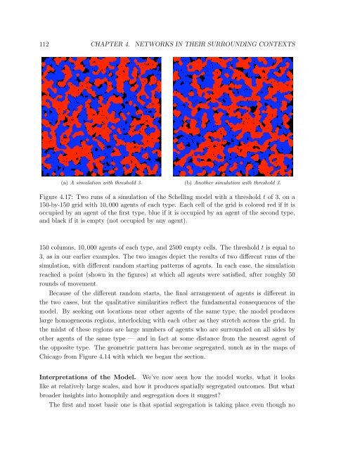
112 CHAPTER 4. NETWORKS IN THEIR SURROUNDING CONTEXTS (a) A simulation with threshold 3. (b) Another simulation with threshold 3. Figure 4.17: Two runs of a simulation of the Schelling model with a threshold t of 3, on a 150-by-150 grid with 10, 000 agents of each type. Each cell of the grid is colored red if it is occupied by an agent of the first type, blue if it is occupied by an agent of the second type, and black if it is empty (not occupied by any agent). 150 columns, 10, 000 agents of each type, and 2500 empty cells. The threshold t is equal to 3, as in our earlier examples. The two images depict the results of two different runs of the simulation, with different random starting patterns of agents. In each case, the simulation reached a point (shown in the figures) at which all agents were satisfied, after roughly 50 rounds of movement. Because of the different random starts, the final arrangement of agents is different in the two cases, but the qualitative similarities reflect the fundamental consequences of the model. By seeking out locations near other agents of the same type, the model produces large homogeneous regions, interlocking with each other as they stretch across the grid. In the midst of these regions are large numbers of agents who are surrounded on all sides by other agents of the same type — and in fact at some distance from the nearest agent of the opposite type. The geometric pattern has become segregated, much as in the maps of Chicago from Figure 4.14 with which we began the section. Interpretations of the Model. We’ve now seen how the model works, what it looks like at relatively large scales, and how it produces spatially segregated outcomes. But what broader insights into homophily and segregation does it suggest? The first and most basic one is that spatial segregation is taking place even though no
4.5. A SPATIAL MODEL OF SEGREGATION 113 X X O X O O X X O O X X O O O X X X X O X X X O O O O X X O O X X Figure 4.18: With a threshold of 3, it is possible to arrange agents in an integrated pattern: all agents are satisfied, and everyone who is not on the boundary on the grid has an equal number of neighbors of each type. individual agent is actively seeking it. Sticking to our focus on a threshold t of 3, we see that although agents want to be near others like them, their requirements are not particularly draconian. For example, an agent would be perfectly happy to be in the minority among its neighbors, with five neighbors of the opposite type and three of its own type. Nor are the requirements globally incompatible with complete integration of the population. By arranging agents in a checkerboard pattern as shown in Figure 4.18, we can make each agent satisfied, and all agents not on the boundary of the grid have exactly four neighbors of each type. This is a pattern that we can continue on as large a grid as we want. Thus, segregation is not happening because we have subtly built it into the model — agents are willing to be in the minority, and they could all be satisfied if we were only able to carefully arrange them in an integrated pattern. The problem is that from a random start, it is very hard for the collection of agents to find such integrated patterns. Much more typically, agents will attach themselves to clusters of others like themselves, and these clusters will grow as other agents follow suit. Moreover, there is a compounding effect as the rounds of movement unfold, in which agents who fall below their threshold depart for more homogeneous parts of the grid, causing previously satisfied agents to fall below their thresholds and move as well — an effect that Schelling describes as the progressive “unraveling” of more integrated regions [366]. In the long run, this process will tend to cause segregated regions to grow at the expense of more integrated ones. The overall effect is one in which the local preferences of individual agents have produced a global pattern that none of them necessarily intended. X O X
- Page 1 and 2: From the book Networks, Crowds, and
- Page 3 and 4: 4.1. HOMOPHILY 87 Figure 4.1: Homop
- Page 5 and 6: 4.1. HOMOPHILY 89 like this [202, 3
- Page 7 and 8: 4.2. MECHANISMS UNDERLYING HOMOPHIL
- Page 9 and 10: 4.3. AFFILIATION 93 Anna Daniel Lit
- Page 11 and 12: 4.3. AFFILIATION 95 graphs are ofte
- Page 13 and 14: 4.4. TRACKING LINK FORMATION IN ON-
- Page 15 and 16: 4.4. TRACKING LINK FORMATION IN ON-
- Page 17 and 18: 4.4. TRACKING LINK FORMATION IN ON-
- Page 19 and 20: 4.4. TRACKING LINK FORMATION IN ON-
- Page 21 and 22: 4.4. TRACKING LINK FORMATION IN ON-
- Page 23 and 24: 4.5. A SPATIAL MODEL OF SEGREGATION
- Page 25 and 26: 4.5. A SPATIAL MODEL OF SEGREGATION
- Page 27: 4.5. A SPATIAL MODEL OF SEGREGATION
- Page 31 and 32: 4.5. A SPATIAL MODEL OF SEGREGATION
- Page 33 and 34: 4.6. EXERCISES 117 seven people in
112 CHAPTER 4. NETWORKS IN THEIR SURROUNDING CONTEXTS<br />
(a) A simulation with threshold 3. (b) Another simulation with threshold 3.<br />
Figure 4.17: Two runs of a simulation of the Schell<strong>in</strong>g model with a threshold t of 3, on a<br />
150-by-150 grid with 10, 000 agents of each type. Each cell of the grid is colored red if it is<br />
occupied by an agent of the first type, blue if it is occupied by an agent of the second type,<br />
and black if it is empty (not occupied by any agent).<br />
150 columns, 10, 000 agents of each type, and 2500 empty cells. The threshold t is equal to<br />
3, as <strong>in</strong> our earlier examples. The two images depict the results of two different runs of the<br />
simulation, with different random start<strong>in</strong>g patterns of agents. In each case, the simulation<br />
reached a po<strong>in</strong>t (shown <strong>in</strong> the figures) at which all agents were satisfied, after roughly 50<br />
rounds of movement.<br />
Because of the different random starts, the f<strong>in</strong>al arrangement of agents is different <strong>in</strong><br />
the two cases, but the qualitative similarities reflect the fundamental consequences of the<br />
model. By seek<strong>in</strong>g out locations near other agents of the same type, the model produces<br />
large homogeneous regions, <strong>in</strong>terlock<strong>in</strong>g with each other as they stretch across the grid. In<br />
the midst of these regions are large numbers of agents who are surrounded on all sides by<br />
other agents of the same type — and <strong>in</strong> fact at some distance from the nearest agent of<br />
the opposite type. The geometric pattern has become segregated, much as <strong>in</strong> the maps of<br />
Chicago from Figure 4.14 with which we began the section.<br />
Interpretations of the Model. We’ve now seen how the model works, what it looks<br />
like at relatively large scales, and how it produces spatially segregated outcomes. But what<br />
broader <strong>in</strong>sights <strong>in</strong>to homophily and segregation does it suggest?<br />
The first and most basic one is that spatial segregation is tak<strong>in</strong>g place even though no


