Chapter 4 Networks in Their Surrounding Contexts - Cornell University
Chapter 4 Networks in Their Surrounding Contexts - Cornell University
Chapter 4 Networks in Their Surrounding Contexts - Cornell University

Create successful ePaper yourself
Turn your PDF publications into a flip-book with our unique Google optimized e-Paper software.
From the book <strong>Networks</strong>, Crowds, and Markets: Reason<strong>in</strong>g about a Highly Connected World.<br />
By David Easley and Jon Kle<strong>in</strong>berg. Cambridge <strong>University</strong> Press, 2010.<br />
Complete prepr<strong>in</strong>t on-l<strong>in</strong>e at http://www.cs.cornell.edu/home/kle<strong>in</strong>ber/networks-book/<br />
<strong>Chapter</strong> 4<br />
<strong>Networks</strong> <strong>in</strong> <strong>Their</strong> Surround<strong>in</strong>g<br />
<strong>Contexts</strong><br />
In <strong>Chapter</strong> 3 we considered some of the typical structures that characterize social networks,<br />
and some of the typical processes that affect the formation of l<strong>in</strong>ks <strong>in</strong> the network. Our<br />
discussion there focused primarily on the network as an object of study <strong>in</strong> itself, relatively<br />
<strong>in</strong>dependent of the broader world <strong>in</strong> which it exists.<br />
However, the contexts <strong>in</strong> which a social network is embedded will generally have significant<br />
effects on its structure, Each <strong>in</strong>dividual <strong>in</strong> a social network has a dist<strong>in</strong>ctive set of<br />
personal characteristics, and similarities and compatibilities among two people’s characteristics<br />
can strongly <strong>in</strong>fluence whether a l<strong>in</strong>k forms between them. Each <strong>in</strong>dividual also engages<br />
<strong>in</strong> a set of behaviors and activities that can shape the formation of l<strong>in</strong>ks with<strong>in</strong> the network.<br />
These considerations suggest what we mean by a network’s surround<strong>in</strong>g contexts: factors<br />
that exist outside the nodes and edges of a network, but which nonetheless affect how the<br />
network’s structure evolves.<br />
In this chapter we consider how such effects operate, and what they imply about the<br />
structure of social networks. Among other observations, we will f<strong>in</strong>d that the surround<strong>in</strong>g<br />
contexts affect<strong>in</strong>g a network’s formation can, to some extent, be viewed <strong>in</strong> network terms as<br />
well — and by expand<strong>in</strong>g the network to represent the contexts together with the <strong>in</strong>dividuals,<br />
we will see <strong>in</strong> fact that several different processes of network formation can be described <strong>in</strong><br />
a common framework.<br />
Draft version: June 10, 2010<br />
85
86 CHAPTER 4. NETWORKS IN THEIR SURROUNDING CONTEXTS<br />
4.1 Homophily<br />
One of the most basic notions govern<strong>in</strong>g the structure of social networks is homophily — the<br />
pr<strong>in</strong>ciple that we tend to be similar to our friends. Typically, your friends don’t look like a<br />
random sample of the underly<strong>in</strong>g population: viewed collectively, your friends are generally<br />
similar to you along racial and ethnic dimensions; they are similar <strong>in</strong> age; and they are also<br />
similar <strong>in</strong> characteristics that are more or less mutable, <strong>in</strong>clud<strong>in</strong>g the places they live, their<br />
occupations, their levels of affluence, and their <strong>in</strong>terests, beliefs, and op<strong>in</strong>ions. Clearly most<br />
of us have specific friendships that cross all these boundaries; but <strong>in</strong> aggregate, the pervasive<br />
fact is that l<strong>in</strong>ks <strong>in</strong> a social network tend to connect people who are similar to one another.<br />
This observation has a long history; as McPherson, Smith-Lov<strong>in</strong>, and Cook note <strong>in</strong><br />
their extensive review of research on homophily [294], the underly<strong>in</strong>g idea can be found <strong>in</strong><br />
writ<strong>in</strong>gs of Plato (“similarity begets friendship”) and Aristotle (people “love those who are<br />
like themselves”), as well as <strong>in</strong> proverbs such as “birds of a feather flock together.” Its role<br />
<strong>in</strong> modern sociological research was catalyzed <strong>in</strong> large part by <strong>in</strong>fluential work of Lazarsfeld<br />
and Merton <strong>in</strong> the 1950s [269].<br />
Homophily provides us with a first, fundamental illustration of how a network’s surround<strong>in</strong>g<br />
contexts can drive the formation of its l<strong>in</strong>ks. Consider the basic contrast between<br />
a friendship that forms because two people are <strong>in</strong>troduced through a common friend and<br />
a friendship that forms because two people attend the same school or work for the same<br />
company. In the first case, a new l<strong>in</strong>k is added for reasons that are <strong>in</strong>tr<strong>in</strong>sic to the network<br />
itself; we need not look beyond the network to understand where the l<strong>in</strong>k came from. In<br />
the second case, the new l<strong>in</strong>k arises for an equally natural reason, but one that makes sense<br />
only when we look at the contextual factors beyond the network — at some of the social<br />
environments (<strong>in</strong> this case schools and companies) to which the nodes belong.<br />
Often, when we look at a network, such contexts capture some of the dom<strong>in</strong>ant features<br />
of its overall structure. Figure 4.1, for example, depicts the social network with<strong>in</strong> a<br />
particular town’s middle school and high school (encompass<strong>in</strong>g grades 7-12) [304]; <strong>in</strong> this<br />
image, produced by the study’s author James Moody, students of different races are drawn<br />
as differently-colored circles. Two dom<strong>in</strong>ant divisions with<strong>in</strong> the network are apparent. One<br />
division is based on race (from left to right <strong>in</strong> the figure); the other, based on age and school<br />
attendance, separates students <strong>in</strong> the middle school from those <strong>in</strong> the high school (from top<br />
to bottom <strong>in</strong> the figure). There are many other structural details <strong>in</strong> this network, but the<br />
effects of these two contexts stand out when the network is viewed at a global level.<br />
Of course, there are strong <strong>in</strong>teractions between <strong>in</strong>tr<strong>in</strong>sic and contextual effects on the<br />
formation of any s<strong>in</strong>gle l<strong>in</strong>k; they are both operat<strong>in</strong>g concurrently <strong>in</strong> the same network. For<br />
example, the pr<strong>in</strong>ciple of triadic closure — that triangles <strong>in</strong> the network tend to “close”<br />
as l<strong>in</strong>ks form between friends of friends — is supported by a range of mechanisms that<br />
range from the <strong>in</strong>tr<strong>in</strong>sic to the contextual. In <strong>Chapter</strong> 3 we motivated triadic closure by
4.1. HOMOPHILY 87<br />
Figure 4.1: Homophily can produce a division of a social network <strong>in</strong>to densely-connected, homogeneous<br />
parts that are weakly connected to each other. In this social network from a town’s middle school and<br />
high school, two such divisions <strong>in</strong> the network are apparent: one based on race (with students of different<br />
races drawn as differently colored circles), and the other based on friendships <strong>in</strong> the middle and high schools<br />
respectively [304].<br />
hypothesiz<strong>in</strong>g <strong>in</strong>tr<strong>in</strong>sic mechanisms: when <strong>in</strong>dividuals B and C have a common friend A,<br />
then there are <strong>in</strong>creased opportunities and sources of trust on which to base their <strong>in</strong>teractions,<br />
and A will also have <strong>in</strong>centives to facilitate their friendship. However, social contexts also<br />
provide natural bases for triadic closure: s<strong>in</strong>ce we know that A-B and A-C friendships<br />
already exist, the pr<strong>in</strong>ciple of homophily suggests that B and C are each likely to be similar<br />
to A <strong>in</strong> a number of dimensions, and hence quite possibly similar to each other as well. As<br />
a result, based purely on this similarity, there is an elevated chance that a B-C friendship<br />
will form; and this is true even if neither of them is aware that the other one knows A.<br />
The po<strong>in</strong>t isn’t that any one basis for triadic closure is the “correct” one. Rather, as we<br />
take <strong>in</strong>to account more and more of the factors that drive the formation of l<strong>in</strong>ks <strong>in</strong> a social
88 CHAPTER 4. NETWORKS IN THEIR SURROUNDING CONTEXTS<br />
Figure 4.2: Us<strong>in</strong>g a numerical measure, one can determ<strong>in</strong>e whether small networks such as<br />
this one (with nodes divided <strong>in</strong>to two types) exhibit homophily.<br />
network, it <strong>in</strong>evitably becomes difficult to attribute any <strong>in</strong>dividual l<strong>in</strong>k to a s<strong>in</strong>gle factor.<br />
And ultimately, one expects most l<strong>in</strong>ks to <strong>in</strong> fact arise from a comb<strong>in</strong>ation of several factors<br />
— partly due to the effect of other nodes <strong>in</strong> the network, and partly due to the surround<strong>in</strong>g<br />
contexts.<br />
Measur<strong>in</strong>g Homophily. When we see strik<strong>in</strong>g divisions with<strong>in</strong> a network like the one <strong>in</strong><br />
Figure 4.1, it is important to ask whether they are “genu<strong>in</strong>ely” present <strong>in</strong> the network itself,<br />
and not simply an artifact of how it is drawn. To make this question concrete, we need to<br />
formulate it more precisely: given a particular characteristic of <strong>in</strong>terest (like race, or age),<br />
is there a simple test we can apply to a network <strong>in</strong> order to estimate whether it exhibits<br />
homophily accord<strong>in</strong>g to this characteristic?<br />
S<strong>in</strong>ce the example <strong>in</strong> Figure 4.1 is too large to <strong>in</strong>spect by hand, let’s consider this question<br />
on a smaller example where we can develop some <strong>in</strong>tuition. Let’s suppose <strong>in</strong> particular that<br />
we have the friendship network of an elementary-school classroom, and we suspect that it<br />
exhibits homophily by gender: boys tend to be friends with boys, and girls tend to be friends<br />
with girls. For example, the graph <strong>in</strong> Figure 4.2 shows the friendship network of a (small)<br />
hypothetical classroom <strong>in</strong> which the three shaded nodes are girls and the six unshaded nodes<br />
are boys. If there were no cross-gender edges at all, then the question of homophily would<br />
be easy to resolve: it would be present <strong>in</strong> an extreme sense. But we expect that homophily<br />
should be a more subtle effect that is visible ma<strong>in</strong>ly <strong>in</strong> aggregate — as it is, for example, <strong>in</strong><br />
the real data from Figure 4.1. Is the picture <strong>in</strong> Figure 4.2 consistent with homophily?<br />
There is a natural numerical measure of homophily that we can use to address questions
4.1. HOMOPHILY 89<br />
like this [202, 319]. To motivate the measure (us<strong>in</strong>g the example of gender as <strong>in</strong> Figure 4.2),<br />
we first ask the follow<strong>in</strong>g question: what would it mean for a network not to exhibit homophily<br />
by gender? It would mean that the proportion of male and female friends a person<br />
has looks like the background male/female distribution <strong>in</strong> the full population. Here’s a<br />
closely related formulation of this “no-homophily” def<strong>in</strong>ition that is a bit easier to analyze:<br />
if we were to randomly assign each node a gender accord<strong>in</strong>g to the gender balance <strong>in</strong> the<br />
real network, then the number of cross-gender edges should not change significantly relative<br />
to what we see <strong>in</strong> the real network. That is, <strong>in</strong> a network with no homophily, friendships are<br />
be<strong>in</strong>g formed as though there were random mix<strong>in</strong>g across the given characteristic.<br />
Thus, suppose we have a network <strong>in</strong> which a p fraction of all <strong>in</strong>dividuals are male, and<br />
a q fraction of all <strong>in</strong>dividuals are female. Consider a given edge <strong>in</strong> this network. If we<br />
<strong>in</strong>dependently assign each node the gender male with probability p and the gender female<br />
with probability q, then both ends of the edge will be male with probability p 2 , and both<br />
ends will be female with probability q 2 . On the other hand, if the first end of the edge is<br />
male and the second end is female, or vice versa, then we have a cross-gender edge, so this<br />
happens with probability 2pq.<br />
So we can summarize the test for homophily accord<strong>in</strong>g to gender as follows:<br />
Homophily Test: If the fraction of cross-gender edges is significantly less than<br />
2pq, then there is evidence for homophily.<br />
In Figure 4.2, for example, 5 of the 18 edges <strong>in</strong> the graph are cross-gender. S<strong>in</strong>ce p =2/3<br />
and q =1/3 <strong>in</strong> this example, we should be compar<strong>in</strong>g the fraction of cross-gender edges to<br />
the quantity 2pq =4/9 = 8/18. In other words, with no homophily, one should expect to<br />
see 8 cross-gender edges rather than than 5, and so this example shows some evidence of<br />
homophily.<br />
There are a few po<strong>in</strong>ts to note here. First, the number of cross-gender edges <strong>in</strong> a random<br />
assignment of genders will deviate some amount from its expected value of 2pq, and so<br />
to perform the test <strong>in</strong> practice one needs a work<strong>in</strong>g def<strong>in</strong>ition of “significantly less than.”<br />
Standard measures of statistical significance (quantify<strong>in</strong>g the significance of a deviation below<br />
a mean) can be used for this purpose. Second, it’s also easily possible for a network to have a<br />
fraction of cross-gender edges that is significantly more than 2pq. In such a case, we say that<br />
the network exhibits <strong>in</strong>verse homophily. The network of romantic relationships <strong>in</strong> Figure 2.7<br />
from <strong>Chapter</strong> 2 is a clear example of this; almost all the relationships reported by the highschool<br />
students <strong>in</strong> the study <strong>in</strong>volved opposite-sex partners, rather than same-sex partners,<br />
so almost all the edges are cross-gender.<br />
F<strong>in</strong>ally, it’s easy to extend our homophily test to any underly<strong>in</strong>g characteristic (race,<br />
ethnicity, age, native language, political orientation, and so forth). When the characteristic<br />
can only take two possible values (say, one’s vot<strong>in</strong>g preference <strong>in</strong> a two-candidate election),<br />
then we can draw a direct analogy to the case of two genders, and use the same formula
90 CHAPTER 4. NETWORKS IN THEIR SURROUNDING CONTEXTS<br />
2pq. When the characteristic can take on more than two possible values, we still perform a<br />
general version of the same calculation. For this, we say that an edge is heterogeneous if it<br />
connects two nodes that are different accord<strong>in</strong>g to the characteristic <strong>in</strong> question. We then ask<br />
how the number of heterogeneous edges compares to what we’d see if we were to randomly<br />
assign values for the characteristic to all nodes <strong>in</strong> the network — us<strong>in</strong>g the proportions from<br />
the real data as probabilities. In this way, even a network <strong>in</strong> which the nodes are classified<br />
<strong>in</strong>to many groups can be tested for homophily us<strong>in</strong>g the same underly<strong>in</strong>g comparison to a<br />
basel<strong>in</strong>e of random mix<strong>in</strong>g.<br />
4.2 Mechanisms Underly<strong>in</strong>g Homophily: Selection and<br />
Social Influence<br />
The fact that people tend to have l<strong>in</strong>ks to others who are similar to them is a statement about<br />
the structure of social networks; on its own, it does not propose an underly<strong>in</strong>g mechanism<br />
by which ties among similar people are preferentially formed.<br />
In the case of immutable characteristics such as race or ethnicity, the tendency of people<br />
to form friendships with others who are like them is often termed selection, <strong>in</strong> that people<br />
are select<strong>in</strong>g friends with similar characteristics. Selection may operate at several different<br />
scales, and with different levels of <strong>in</strong>tentionality. In a small group, when people choose<br />
friends who are most similar from among a clearly del<strong>in</strong>eated pool of potential contacts,<br />
there is clearly active choice go<strong>in</strong>g on. In other cases, and at more global levels, selection<br />
can be more implicit. For example, when people live <strong>in</strong> neighborhoods, attend schools, or<br />
work for companies that are relatively homogeneous compared to the population at large,<br />
the social environment is already favor<strong>in</strong>g opportunities to form friendships with others like<br />
oneself. For this discussion, we will refer to all these effects cumulatively as selection.<br />
When we consider how immutable characteristics <strong>in</strong>teract with network formation, the<br />
order of events is clear: a person’s attributes are determ<strong>in</strong>ed at birth, and they play a<br />
role <strong>in</strong> how this person’s connections are formed over the course of his or her life. With<br />
characteristics that are more mutable, on the other hand — behaviors, activities, <strong>in</strong>terests,<br />
beliefs, and op<strong>in</strong>ions — the feedback effects between people’s <strong>in</strong>dividual characteristics and<br />
their l<strong>in</strong>ks <strong>in</strong> the social network become significantly more complex. The process of selection<br />
still operates, with <strong>in</strong>dividual characteristics affect<strong>in</strong>g the connections that are formed. But<br />
now another process comes <strong>in</strong>to play as well: people may modify their behaviors to br<strong>in</strong>g<br />
them more closely <strong>in</strong>to alignment with the behaviors of their friends. This process has<br />
been variously described as socialization [233] and social <strong>in</strong>fluence [170], s<strong>in</strong>ce the exist<strong>in</strong>g<br />
social connections <strong>in</strong> a network are <strong>in</strong>fluenc<strong>in</strong>g the <strong>in</strong>dividual characteristics of the nodes.<br />
Social <strong>in</strong>fluence can be viewed as the reverse of selection: with selection, the <strong>in</strong>dividual<br />
characteristics drive the formation of l<strong>in</strong>ks, while with social <strong>in</strong>fluence, the exist<strong>in</strong>g l<strong>in</strong>ks <strong>in</strong>
4.2. MECHANISMS UNDERLYING HOMOPHILY: SELECTION AND SOCIAL INFLUENCE91<br />
the network serve to shape people’s (mutable) characteristics. 1<br />
The Interplay of Selection and Social Influence. When we look at a s<strong>in</strong>gle snapshot<br />
of a network and see that people tend to share mutable characteristics with their friends, it<br />
can be very hard to sort out the dist<strong>in</strong>ct effects and relative contributions of selection and<br />
social <strong>in</strong>fluence. Have the people <strong>in</strong> the network adapted their behaviors to become more like<br />
their friends, or have they sought out people who were already like them? Such questions can<br />
be addressed us<strong>in</strong>g longitud<strong>in</strong>al studies of a social network, <strong>in</strong> which the social connections<br />
and the behaviors with<strong>in</strong> a group are both tracked over a period of time. Fundamentally, this<br />
makes it possible to see the behavioral changes that occur after changes <strong>in</strong> an <strong>in</strong>dividual’s<br />
network connections, as opposed to the changes to the network that occur after an <strong>in</strong>dividual<br />
changes his or her behavior.<br />
This type of methodology has been used, for example, to study the processes that lead<br />
pairs of adolescent friends to have similar outcomes <strong>in</strong> terms of scholastic achievement and<br />
del<strong>in</strong>quent behavior such as drug use [92]. Empirical evidence confirms the <strong>in</strong>tuitive fact that<br />
teenage friends are similar to each other <strong>in</strong> their behaviors, and both selection and social<br />
<strong>in</strong>fluence have a natural resonance <strong>in</strong> this sett<strong>in</strong>g: teenagers seek out social circles composed<br />
of people like them, and peer pressure causes them to conform to behavioral patterns with<strong>in</strong><br />
their social circles. What is much harder to resolve is how these two effects <strong>in</strong>teract, and<br />
whether one is more strongly at work than the other. As longitud<strong>in</strong>al behavior relevant to<br />
this question became available, researchers began quantify<strong>in</strong>g the relative impact of these<br />
different factors. A l<strong>in</strong>e of work beg<strong>in</strong>n<strong>in</strong>g with Cohen and Kandel has suggested that while<br />
both effects are present <strong>in</strong> the data, the outsized role that earlier <strong>in</strong>formal arguments had<br />
accorded to peer pressure (i.e. social <strong>in</strong>fluence) is actually more moderate; the effect of<br />
selection here is <strong>in</strong> fact comparable to (and sometimes greater than) the effect of social<br />
<strong>in</strong>fluence [114, 233].<br />
Understand<strong>in</strong>g the tension between these different forces can be important not just for<br />
identify<strong>in</strong>g underly<strong>in</strong>g causes, but also for reason<strong>in</strong>g about the effect of possible <strong>in</strong>terventions<br />
one might attempt <strong>in</strong> the system [21, 396]. For example, once we f<strong>in</strong>d that illicit drug use<br />
displays homophily across a social network — with students show<strong>in</strong>g a greater likelihood to<br />
use drugs when their friends do — we can ask about the effects of a program that targets<br />
certa<strong>in</strong> high-school students and <strong>in</strong>fluences them to stop us<strong>in</strong>g drugs. To the extent that the<br />
observed homophily is based on some amount of social <strong>in</strong>fluence, such a program could have<br />
a broad impact across the social network, by caus<strong>in</strong>g the friends of these targeted students<br />
to stop us<strong>in</strong>g drugs as well. But one must be careful; if the observed homophily is aris<strong>in</strong>g<br />
<strong>in</strong>stead almost entirely from selection effects, then the program may not reduce drug use<br />
1 There are other cognitive effects at work as well; for example, people may systematically misperceive<br />
the characteristics of their friends as be<strong>in</strong>g more <strong>in</strong> alignment with their own than they really are [224]. For<br />
our discussion here, we will not focus explicitly on such effects.
92 CHAPTER 4. NETWORKS IN THEIR SURROUNDING CONTEXTS<br />
beyond the students it directly targets: as these students stop us<strong>in</strong>g drugs, they change<br />
their social circles and form new friendships with students who don’t use drugs, but the<br />
drug-us<strong>in</strong>g behavior of other students is not strongly affected.<br />
Another example of research address<strong>in</strong>g this subtle <strong>in</strong>terplay of factors is the work of<br />
Christakis and Fowler on the effect of social networks on health-related outcomes. In one<br />
recent study, us<strong>in</strong>g longitud<strong>in</strong>al data cover<strong>in</strong>g roughly 12,000 people, they tracked obesity<br />
status and social network structure over a 32-year period [108]. They found that obese and<br />
non-obese people clustered <strong>in</strong> the network <strong>in</strong> a fashion consistent with homophily, accord<strong>in</strong>g<br />
to the numerical measure described <strong>in</strong> Section 4.1: people tend to be more similar <strong>in</strong> obesity<br />
status to their network neighbors than <strong>in</strong> a version of the same network where obesity status<br />
is assigned randomly. The problem is then to dist<strong>in</strong>guish among several hypotheses for why<br />
this cluster<strong>in</strong>g is present: is it<br />
(i) because of selection effects, <strong>in</strong> which people are choos<strong>in</strong>g to form friendships with others<br />
of similar obesity status?<br />
(ii) because of the confound<strong>in</strong>g effects of homophily accord<strong>in</strong>g to other characteristics, <strong>in</strong><br />
which the network structure <strong>in</strong>dicates exist<strong>in</strong>g patterns of similarity <strong>in</strong> other dimensions<br />
that correlate with obesity status? or<br />
(iii) because changes <strong>in</strong> the obesity status of a person’s friends was exert<strong>in</strong>g a (presumably<br />
behavioral) <strong>in</strong>fluence that affected his or her future obesity status?<br />
Statistical analysis <strong>in</strong> Christakis and Fowler’s paper argues that, even account<strong>in</strong>g for effects of<br />
types (i) and (ii), there is significant evidence for an effect of type (iii) as well: that obesity is<br />
a health condition display<strong>in</strong>g a form of social <strong>in</strong>fluence, with changes <strong>in</strong> your friends’ obesity<br />
status <strong>in</strong> turn hav<strong>in</strong>g a subsequent effect on you. This suggests the <strong>in</strong>trigu<strong>in</strong>g prospect that<br />
obesity (and perhaps other health conditions with a strong behavioral aspect) may exhibit<br />
some amount of “contagion” <strong>in</strong> a social sense: you don’t necessarily catch it from your<br />
friends the way you catch the flu, but it nonetheless can spread through the underly<strong>in</strong>g<br />
social network via the mechanism of social <strong>in</strong>fluence.<br />
These examples, and this general style of <strong>in</strong>vestigation, show how careful analysis is<br />
needed to dist<strong>in</strong>guish among different factors contribut<strong>in</strong>g to an aggregate conclusion: even<br />
when people tend to be similar to their neighbors <strong>in</strong> a social network, it may not be clear<br />
why. The po<strong>in</strong>t is that an observation of homophily is often not an endpo<strong>in</strong>t <strong>in</strong> itself, but<br />
rather the start<strong>in</strong>g po<strong>in</strong>t for deeper questions — questions that address why the homophily<br />
is present, how its underly<strong>in</strong>g mechanisms will affect the further evolution of the network,<br />
and how these mechanisms <strong>in</strong>teract with possible outside attempts to <strong>in</strong>fluence the behavior<br />
of people <strong>in</strong> the network.
4.3. AFFILIATION 93<br />
Anna<br />
Daniel<br />
Literacy<br />
Volunteers<br />
Karate<br />
Club<br />
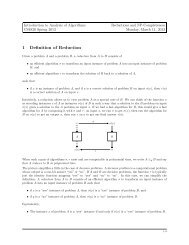
Figure 4.3: An affiliation network is a bipartite graph that shows which <strong>in</strong>dividuals are<br />
affiliated with which groups or activities. Here, Anna participates <strong>in</strong> both of the social foci<br />
on the right, while Daniel participates <strong>in</strong> only one.<br />
4.3 Affiliation<br />
Thus far, we have been discuss<strong>in</strong>g contextual factors that affect the formation of l<strong>in</strong>ks <strong>in</strong><br />
a network — based on similarities <strong>in</strong> characteristics of the nodes, and based on behaviors<br />
and activities that the nodes engage <strong>in</strong>. These surround<strong>in</strong>g contexts have been viewed,<br />
appropriately, as exist<strong>in</strong>g “outside” the network. But <strong>in</strong> fact, it’s possible to put these<br />
contexts <strong>in</strong>to the network itself, by work<strong>in</strong>g with a larger network that conta<strong>in</strong>s both people<br />
and contexts as nodes. Through such a network formulation, we will get additional <strong>in</strong>sight<br />
<strong>in</strong>to some broad aspects of homophily, and see how the simultaneous evolution of contexts<br />
and friendships can be put on a common network foot<strong>in</strong>g with the notion of triadic closure<br />
from <strong>Chapter</strong> 3.<br />
In pr<strong>in</strong>ciple we could represent any context this way, but for the sake of concreteness we’ll<br />
focus on how to represent the set of activities a person takes part <strong>in</strong>, and how these affect<br />
the formation of l<strong>in</strong>ks. We will take a very general view of the notion of an “activity” here.<br />
Be<strong>in</strong>g part of a particular company, organization, or neigborhood; frequent<strong>in</strong>g a particular<br />
place; pursu<strong>in</strong>g a particular hobby or <strong>in</strong>terest — these are all activities that, when shared<br />
between two people, tend to <strong>in</strong>crease the likelihood that they will <strong>in</strong>teract and hence form a<br />
l<strong>in</strong>k <strong>in</strong> the social network [78, 161]. Adopt<strong>in</strong>g term<strong>in</strong>ology due to Scott Feld, we’ll refer to<br />
such activities as foci — that is, “focal po<strong>in</strong>ts” of social <strong>in</strong>teraction — constitut<strong>in</strong>g “social,<br />
psychological, legal, or physical entit[ies] around which jo<strong>in</strong>t activities are organized (e.g.<br />
workplaces, voluntary organizations, hangouts, etc.)” [161].<br />
Affiliation <strong>Networks</strong>. As a first step, we can represent the participation of a set of people<br />
<strong>in</strong> a set of foci us<strong>in</strong>g a graph as follows. We will have a node for each person, and a node<br />
for each focus, and we will connect person A to focus X by an edge if A participates <strong>in</strong> X.
94 CHAPTER 4. NETWORKS IN THEIR SURROUNDING CONTEXTS<br />
John<br />
Doerr<br />
Shirley<br />
Tilghman<br />
Arthur<br />
Lev<strong>in</strong>son<br />
Al Gore<br />
Steve<br />
Jobs<br />
Andrea<br />
Jung<br />
Susan<br />
Hockfield<br />
Amazon<br />
Google<br />
Apple<br />
Disney<br />
General<br />
Electric<br />
Figure 4.4: One type of affiliation network that has been widely studied is the memberships<br />
of people on corporate boards of directors [301]. A very small portion of this network (as of<br />
mid-2009) is shown here. The structural pattern of memberships can reveal subtleties <strong>in</strong> the<br />
<strong>in</strong>teractions among both the board members and the companies.<br />
A very simple example of such a graph is depicted <strong>in</strong> Figure 4.3, show<strong>in</strong>g two people (Anna<br />
and Daniel) and two foci (work<strong>in</strong>g for a literacy tutor<strong>in</strong>g organization, and belong<strong>in</strong>g to a<br />
karate club). The graph <strong>in</strong>dicates that Anna participates <strong>in</strong> both of the foci, while Daniel<br />
participates <strong>in</strong> only one.<br />
We will refer to such a graph as an affiliation network, s<strong>in</strong>ce it represents the affiliation of<br />
people (drawn on the left) with foci (drawn on the right) [78, 323]. More generally, affiliation<br />
networks are examples of a class of graphs called bipartite graphs. We say that a graph is<br />
bipartite if its nodes can be divided <strong>in</strong>to two sets <strong>in</strong> such a way that every edge connects a<br />
node <strong>in</strong> one set to a node <strong>in</strong> the other set. (In other words, there are no edges jo<strong>in</strong><strong>in</strong>g a pair<br />
of nodes that belong to the same set; all edges go between the two sets.) Bipartite graphs<br />
are very useful for represent<strong>in</strong>g data <strong>in</strong> which the items under study come <strong>in</strong> two categories,<br />
and we want to understand how the items <strong>in</strong> one category are associated with the items<br />
<strong>in</strong> the other. In the case of affiliation networks, the two categories are the people and the<br />
foci, with each edge connect<strong>in</strong>g a person to a focus that he or she participates <strong>in</strong>. Bipartite
4.3. AFFILIATION 95<br />
graphs are often drawn as <strong>in</strong> Figure 4.3, with the two different sets of nodes drawn as two<br />
parallel vertical columns, and the edges cross<strong>in</strong>g between the two columns.<br />
Affiliation networks are studied <strong>in</strong> a range of sett<strong>in</strong>gs where researchers want to understand<br />
the patterns of participation <strong>in</strong> structured activities. As one example, they have<br />
received considerable attention <strong>in</strong> study<strong>in</strong>g the composition of boards of directors of major<br />
corporations [301]. Boards of directors are relatively small advisory groups populated by<br />
high-status <strong>in</strong>dividuals; and s<strong>in</strong>ce many people serve on multiple boards, the overlaps <strong>in</strong><br />
their participation have a complex structure. These overlaps can be naturally represented<br />
by an affiliation network; as the example <strong>in</strong> Figure 4.4 shows, there is a node for each person<br />
and a node for each board, and each edge connects a person to a board that they belong to.<br />
Affiliation networks def<strong>in</strong>ed by boards of directors have the potential to reveal <strong>in</strong>terest<strong>in</strong>g<br />
relationships on both sides of the graph. Two companies are implicitly l<strong>in</strong>ked by hav<strong>in</strong>g<br />
the same person sit on both their boards; we can thus learn about possible conduits for<br />
<strong>in</strong>formation and <strong>in</strong>fluence to flow between different companies. Two people, on the other<br />
hand, are implicitly l<strong>in</strong>ked by serv<strong>in</strong>g together on a board, and so we learn about particular<br />
patterns of social <strong>in</strong>teraction among some of the most powerful members of society. Of<br />
course, even the complete affiliation network of people and boards (of which Figure 4.4<br />
is only a small piece) still misses other important contexts that these people <strong>in</strong>habit; for<br />
example, the seven people <strong>in</strong> Figure 4.4 <strong>in</strong>clude the presidents of two major universities and<br />
a former Vice-President of the United States. 2<br />
Co-Evolution of Social and Affiliation <strong>Networks</strong>. It’s clear that both social networks<br />
and affiliation networks change over time: new friendship l<strong>in</strong>ks are formed, and people<br />
become associated with new foci. Moreover, these changes represent a k<strong>in</strong>d of co-evolution<br />
that reflects the <strong>in</strong>terplay between selection and social <strong>in</strong>fluence: if two people participate <strong>in</strong><br />
a shared focus, this provides them with an opportunity to become friends; and if two people<br />
are friends, they can <strong>in</strong>fluence each other’s choice of foci.<br />
There is a natural network perspective on these ideas, which beg<strong>in</strong>s from a network<br />
representation that slightly extends the notion of an affiliation network. As before, we’ll<br />
have nodes for people and nodes for foci, but we now <strong>in</strong>troduce two dist<strong>in</strong>ct k<strong>in</strong>ds of edges<br />
as well. The first k<strong>in</strong>d of edge functions as an edge <strong>in</strong> a social network: it connects two<br />
2 The structure of this network changes over time as well, and sometimes <strong>in</strong> ways that re<strong>in</strong>force the po<strong>in</strong>ts <strong>in</strong><br />
our present discussion. For example, the board memberships shown <strong>in</strong> Figure 4.4 are taken from the middle<br />
of 2009; by the end of 2009, Arthur Lev<strong>in</strong>son had resigned from the board of directors of Google (thus<br />
remov<strong>in</strong>g one edge from the graph). As part of the news coverage of this resignation, the chair of the U.S.<br />
Federal Trade Commission, Jon Leibowitz, explicitly <strong>in</strong>voked the notion of overlaps <strong>in</strong> board membership,<br />
say<strong>in</strong>g, “Google, Apple and Mr. Lev<strong>in</strong>son should be commended for recogniz<strong>in</strong>g that overlapp<strong>in</strong>g board<br />
members between compet<strong>in</strong>g companies raise serious antitrust issues, and for their will<strong>in</strong>gness to resolve our<br />
concerns without the need for litigation. Beyond this matter, we will cont<strong>in</strong>ue to monitor companies that<br />
share board members and take enforcement actions where appropriate” [219].
96 CHAPTER 4. NETWORKS IN THEIR SURROUNDING CONTEXTS<br />
Claire<br />
Bob<br />
Anna<br />
Karate<br />
Club<br />
Literacy<br />
Volunteers<br />
Daniel<br />
Figure 4.5: A social-affiliation network shows both the friendships between people and their<br />
affiliation with different social foci.<br />
people, and <strong>in</strong>dicates friendship (or alternatively some other social relation, like professional<br />
collaboration). The second k<strong>in</strong>d of edge functions as an edge <strong>in</strong> an affiliation network: it<br />
connects a person to a focus, and <strong>in</strong>dicates the participation of the person <strong>in</strong> the focus. We<br />
will call such a network a social-affiliation network, reflect<strong>in</strong>g the fact that it simultaneously<br />
conta<strong>in</strong>s a social network on the people and an affiliation network on the people and foci.<br />
Figure 4.5 depicts a simple social-affiliation network.<br />
Once we have social-affiliation networks as our representation, we can appreciate that<br />
a range of different mechanisms for l<strong>in</strong>k formation can all be viewed as types of closure<br />
processes, <strong>in</strong> that they <strong>in</strong>volve “clos<strong>in</strong>g” the third edge of a triangle <strong>in</strong> the network. In<br />
particular, suppose we have two nodes B and C with a common neighbor A <strong>in</strong> the network,<br />
and suppose that an edge forms between B and C. There are several <strong>in</strong>terpretations for<br />
what this corresponds to, depend<strong>in</strong>g on whether A, B, and C are people or foci.<br />
(i) If A, B, and C each represent a person, then the formation of the l<strong>in</strong>k between B and<br />
C is triadic closure, just as <strong>in</strong> <strong>Chapter</strong> 3. (See Figure 4.6(a).)<br />
(ii) If B and C represent people, but A represents a focus, then this is someth<strong>in</strong>g different:<br />
it is the tendency of two people to form a l<strong>in</strong>k when they have a focus <strong>in</strong> common. (See<br />
Figure 4.6(b).) This is an aspect of the more general pr<strong>in</strong>ciple of selection, form<strong>in</strong>g<br />
l<strong>in</strong>ks to others who share characteristics with you. To emphasize the analogy with<br />
triadic closure, this process has been called focal closure [259].<br />
(iii) If A and B are people, and C is a focus, then we have the formation of a new affiliation:<br />
B takes part <strong>in</strong> a focus that her friend A is already <strong>in</strong>volved <strong>in</strong>. (See Figure 4.6(c).)<br />
This is a k<strong>in</strong>d of social <strong>in</strong>fluence, <strong>in</strong> which B’s behavior comes <strong>in</strong>to closer alignment
4.4. TRACKING LINK FORMATION IN ON-LINE DATA 97<br />
person<br />
B<br />
A<br />
person<br />
(a) Triadic closure<br />
person<br />
B<br />
C<br />
person<br />
A<br />
person<br />
person<br />
B<br />
(c) Membership closure<br />
A<br />
focus<br />
(b) Focal closure<br />
Figure 4.6: Each of triadic closure, focal closure, and membership closure corresponds to the<br />
clos<strong>in</strong>g of a triangle <strong>in</strong> a social-affiliation network.<br />
C<br />
focus<br />
C<br />
person<br />
with that of her friend A. Cont<strong>in</strong>u<strong>in</strong>g the analogy with triadic closure, we will refer to<br />
this k<strong>in</strong>d of l<strong>in</strong>k formation as membership closure.<br />
Thus, three very different underly<strong>in</strong>g mechanisms — reflect<strong>in</strong>g triadic closure and aspects<br />
of selection and social <strong>in</strong>fluence — can be unified <strong>in</strong> this type of network as k<strong>in</strong>ds of closure:<br />
the formation of a l<strong>in</strong>k <strong>in</strong> cases where the two endpo<strong>in</strong>ts already have a neighbor <strong>in</strong> common.<br />
Figure 4.7 shows all three k<strong>in</strong>ds of closure processes at work: triadic closure leads to a new<br />
l<strong>in</strong>k between Anna and Claire; focal closure leads to a new l<strong>in</strong>k between Anna and Daniel;<br />
and membership closure leads to Bob’s affiliation with the karate club. Oversimplify<strong>in</strong>g the<br />
mechanisms at work, they can be summarized <strong>in</strong> the follow<strong>in</strong>g succ<strong>in</strong>ct way:<br />
(i) Bob <strong>in</strong>troduces Anna to Claire.<br />
(ii) Karate <strong>in</strong>troduces Anna to Daniel.<br />
(iii) Anna <strong>in</strong>troduces Bob to Karate.<br />
4.4 Track<strong>in</strong>g L<strong>in</strong>k Formation <strong>in</strong> On-L<strong>in</strong>e Data<br />
In this chapter and the previous one, we have identified a set of different mechanisms that<br />
lead to the formation of l<strong>in</strong>ks <strong>in</strong> social networks. These mechansisms are good examples
98 CHAPTER 4. NETWORKS IN THEIR SURROUNDING CONTEXTS<br />
Claire<br />
Bob<br />
Anna<br />
Karate<br />
Club<br />
Literacy<br />
Volunteers<br />
Daniel<br />
Figure 4.7: In a social-affiliation network conta<strong>in</strong><strong>in</strong>g both people and foci, edges can form<br />
under the effect of several different k<strong>in</strong>ds of closure processes: two people with a friend <strong>in</strong><br />
common, two people with a focus <strong>in</strong> common, or a person jo<strong>in</strong><strong>in</strong>g a focus that a friend is<br />
already <strong>in</strong>volved <strong>in</strong>.<br />
of social phenomena which are clearly at work <strong>in</strong> small-group sett<strong>in</strong>gs, but which have<br />
traditionally been very hard to measure quantitatively. A natural research strategy is to<br />
try track<strong>in</strong>g these mechanisms as they operate <strong>in</strong> large populations, where an accumulation<br />
of many small effects can produce someth<strong>in</strong>g observable <strong>in</strong> the aggregate. However, given<br />
that most of the forces responsible for l<strong>in</strong>k formation go largely unrecorded <strong>in</strong> everyday life,<br />
it is a challenge to select a large, clearly del<strong>in</strong>eated group of people (and social foci), and<br />
accurately quantify the relative contributions that these different mechanisms make to the<br />
formation of real network l<strong>in</strong>ks.<br />
The availability of data from large on-l<strong>in</strong>e sett<strong>in</strong>gs with clear social structure has made<br />
it possible to attempt some prelim<strong>in</strong>ary research along these l<strong>in</strong>es. As we emphasized <strong>in</strong><br />
<strong>Chapter</strong> 2, any analysis of social processes based on such on-l<strong>in</strong>e datasets must come with<br />
a number of caveats. In particular, it is never a priori clear how much one can extrapolate<br />
from digital <strong>in</strong>teractions to <strong>in</strong>teractions that are not computer-mediated, or even from one<br />
computer-mediated sett<strong>in</strong>g to another. Of course, this problem of extrapolation is present<br />
whenever one studies phenomena <strong>in</strong> a model system, on-l<strong>in</strong>e or not, and the k<strong>in</strong>ds of measurements<br />
these large datasets enable represent <strong>in</strong>terest<strong>in</strong>g first steps toward a deeper quantitative<br />
understand<strong>in</strong>g of how mechanisms of l<strong>in</strong>k formation operate <strong>in</strong> real life. Explor<strong>in</strong>g<br />
these questions <strong>in</strong> a broader range of large datasets is an important problem, and one that<br />
will become easier as large-scale data becomes <strong>in</strong>creas<strong>in</strong>gly abundant.<br />
Triadic closure. With this background <strong>in</strong> m<strong>in</strong>d, let’s start with some questions about<br />
triadic closure. Here’s a first, basic numerical question: how much more likely is a l<strong>in</strong>k to
4.4. TRACKING LINK FORMATION IN ON-LINE DATA 99<br />
Esther<br />
Claire<br />
Bob<br />
Karate<br />
Club<br />
Anna<br />
Daniel<br />
Frank<br />
Grace<br />
Literacy<br />
Volunteers<br />
Figure 4.8: A larger network that conta<strong>in</strong>s the example from Figure 4.7. Pairs of people can<br />
have more than one friend (or more than one focus) <strong>in</strong> common; how does this <strong>in</strong>crease the<br />
likelihood that an edge will form between them?<br />
form between two people <strong>in</strong> a social network if they already have a friend <strong>in</strong> common? (In<br />
other words, how much more likely is a l<strong>in</strong>k to form if it has the effect of clos<strong>in</strong>g a triangle?)<br />
Here’s a second question, along the same l<strong>in</strong>es as the first: How much more likely is an<br />
edge to form between two people if they have multiple friends <strong>in</strong> common? For example,<br />
<strong>in</strong> Figure 4.8, Anna and Esther have two friends <strong>in</strong> common, while Claire and Daniel only<br />
have one friend <strong>in</strong> common. How much more likely is the formation of a l<strong>in</strong>k <strong>in</strong> the first of<br />
these two cases? If we go back to the arguments for why triadic closure operates <strong>in</strong> social<br />
networks, we see that they all are qualitatively strengthened as two people have more friends<br />
<strong>in</strong> common: there are more sources of opportunity and trust for the <strong>in</strong>teraction, there are<br />
more people with an <strong>in</strong>centive to br<strong>in</strong>g them together, and the evidence for homophily is<br />
arguably stronger.<br />
We can address these questions empirically us<strong>in</strong>g network data as follows.<br />
(i) We take two snapshots of the network at different times.<br />
(ii) For each k, we identify all pairs of nodes who have exactly k friends <strong>in</strong> common <strong>in</strong> the<br />
first snapshot, but who are not directly connected by an edge.<br />
(iii) We def<strong>in</strong>e T (k) to be the fraction of these pairs that have formed an edge by the time
100 CHAPTER 4. NETWORKS IN THEIR SURROUNDING CONTEXTS<br />
prob. of l<strong>in</strong>k formation<br />
0.006<br />
0.005<br />
0.004<br />
0.003<br />
0.002<br />
0.001<br />
0<br />
0 2 4 6 8 10<br />
Number of common friends<br />
Figure 4.9: Quantify<strong>in</strong>g the effects of triadic closure <strong>in</strong> an e-mail dataset [259]. The curve<br />
determ<strong>in</strong>ed from the data is shown <strong>in</strong> the solid black l<strong>in</strong>e; the dotted curves show a comparison<br />
to probabilities computed accord<strong>in</strong>g to two simple basel<strong>in</strong>e models <strong>in</strong> which common<br />
friends provide <strong>in</strong>dependent probabilities of l<strong>in</strong>k formation.<br />
of the second snapshot. This is our empirical estimate for the probability that a l<strong>in</strong>k<br />
will form between two people with k friends <strong>in</strong> common.<br />
(iv) We plot T (k) as a function of k to illustrate the effect of common friends on the<br />
formation of l<strong>in</strong>ks.<br />
Note that T (0) is the rate at which l<strong>in</strong>k formation happens when it does not close a triangle,<br />
while the values of T (k) for larger k determ<strong>in</strong>e the rate at which l<strong>in</strong>k formation happens<br />
when it does close a triangle. Thus, the comparison between T (0) and these other values<br />
addresses the most basic question about the power of triadic closure.<br />
Koss<strong>in</strong>ets and Watts computed this function T (k) us<strong>in</strong>g a dataset encod<strong>in</strong>g the full history<br />
of e-mail communication among roughly 22,000 undergraduate and graduate students over<br />
a one-year period at a large U.S. university [259]. This is a “who-talks-to-whom” type of<br />
dataset, as we discussed <strong>in</strong> <strong>Chapter</strong> 2; from the communication traces, Koss<strong>in</strong>ets and Watts<br />
constructed a network that evolved over time, jo<strong>in</strong><strong>in</strong>g two people by a l<strong>in</strong>k at a given <strong>in</strong>stant<br />
if they had exchanged e-mail <strong>in</strong> each direction at some po<strong>in</strong>t <strong>in</strong> the past 60 days. They then<br />
determ<strong>in</strong>ed an “average” version of T (k) by tak<strong>in</strong>g multiple pairs of snapshots: they built<br />
a curve for T (k) on each pair of snapshots us<strong>in</strong>g the procedure described above, and then
4.4. TRACKING LINK FORMATION IN ON-LINE DATA 101<br />
averaged all the curves they obta<strong>in</strong>ed. In particular, the observations <strong>in</strong> each snapshot were<br />
one day apart, so their computation gives the average probability that two people form a<br />
l<strong>in</strong>k per day, as a function of the number of common friends they have.<br />
Figure 4.9 shows a plot of this curve (<strong>in</strong> the solid black l<strong>in</strong>e). The first th<strong>in</strong>g one notices<br />
is the clear evidence for triadic closure: T (0) is very close to 0, after which the probability<br />
of l<strong>in</strong>k formation <strong>in</strong>creases steadily as the number of common friends <strong>in</strong>creases. Moreover,<br />
for much of the plot, this probability <strong>in</strong>creases <strong>in</strong> a roughly l<strong>in</strong>ear fashion as a function<br />
of the number of common friends, with an upward bend away from a straight-l<strong>in</strong>e shape.<br />
The curve turns upward <strong>in</strong> a particularly pronounced way from 0 to 1 to 2 friends: hav<strong>in</strong>g<br />
two common friends produces significantly more than twice the effect on l<strong>in</strong>k formation<br />
compared to hav<strong>in</strong>g a s<strong>in</strong>gle common friend. (The upward effect from 8 to 9 to 10 friends is<br />
also significant, but it occurs on a much smaller sub-population, s<strong>in</strong>ce many fewer people <strong>in</strong><br />
the data have this many friends <strong>in</strong> common without hav<strong>in</strong>g already formed a l<strong>in</strong>k.)<br />
To <strong>in</strong>terpret this plot more deeply, it helps to compare it to an <strong>in</strong>tentionally simplified<br />
basel<strong>in</strong>e model, describ<strong>in</strong>g what one might have expected the data to look like <strong>in</strong> the presence<br />
of triadic closure. Suppose that for some small probability p, each common friend that two<br />
people have gives them an <strong>in</strong>dependent probability p of form<strong>in</strong>g a l<strong>in</strong>k each day. So if two<br />
people have k friends <strong>in</strong> common, the probability they fail to form a l<strong>in</strong>k on any given day is<br />
(1 − p) k : this is because each common friend fails to cause the l<strong>in</strong>k to form with probability<br />
1 − p, and these k trials are <strong>in</strong>dependent. S<strong>in</strong>ce (1 − p) k is the probability the l<strong>in</strong>k fails<br />
to form on a given day, the probability that it does form, accord<strong>in</strong>g to our simple basel<strong>in</strong>e<br />
model, is<br />
Tbasel<strong>in</strong>e(k) = 1 − (1 − p) k .<br />
We plot this curve <strong>in</strong> Figure 4.9 as the upper dotted l<strong>in</strong>e. Given the small absolute effect of<br />
the first common friend <strong>in</strong> the data, we also show a comparison to the curve 1 − (1 − p) k−1 ,<br />
which just shifts the simple basel<strong>in</strong>e curve one unit to the right. Aga<strong>in</strong>, the po<strong>in</strong>t is not to<br />
propose this basel<strong>in</strong>e as an explanatory mechanism for triadic closure, but rather to look at<br />
how the real data compares to it. Both the real curve and the basel<strong>in</strong>e curve are close to<br />
l<strong>in</strong>ear, and hence qualitatively similar; but the fact that the real data turns upward while the<br />
basel<strong>in</strong>e curve turns slightly downward <strong>in</strong>dicates that the assumption of <strong>in</strong>dependent effects<br />
from common friends is too simple to be fully supported by the data.<br />
A still larger and more detailed study of these effects was conducted by Leskovec et<br />
al. [272], who analyzed properties of triadic closure <strong>in</strong> the on-l<strong>in</strong>e social networks of L<strong>in</strong>kedIn,<br />
Flickr, Del.icio.us, and Yahoo! Answers. It rema<strong>in</strong>s an <strong>in</strong>terest<strong>in</strong>g question to try understand<strong>in</strong>g<br />
the similarities and variations <strong>in</strong> triadic closure effects across social <strong>in</strong>teraction <strong>in</strong><br />
a range of different sett<strong>in</strong>gs.
102 CHAPTER 4. NETWORKS IN THEIR SURROUNDING CONTEXTS<br />
prob. of l<strong>in</strong>k formation<br />
0.0005<br />
0.0004<br />
0.0003<br />
0.0002<br />
0.0001<br />
0<br />
0 1 2 3 4 5<br />
number of common foci<br />
Figure 4.10: Quantify<strong>in</strong>g the effects of focal closure <strong>in</strong> an e-mail dataset [259]. Aga<strong>in</strong>, the<br />
curve determ<strong>in</strong>ed from the data is shown <strong>in</strong> the solid black l<strong>in</strong>e, while the dotted curve<br />
provides a comparison to a simple basel<strong>in</strong>e.<br />
Focal and Membership Closure. Us<strong>in</strong>g the same approach, we can compute probabilities<br />
for the other k<strong>in</strong>ds of closure discussed earlier — specifically,<br />
• focal closure: what is the probability that two people form a l<strong>in</strong>k as a function of the<br />
number of foci they are jo<strong>in</strong>tly affiliated with?<br />
• membership closure: what is the probability that a person becomes <strong>in</strong>volved with a<br />
particular focus as a function of the number of friends who are already <strong>in</strong>volved <strong>in</strong> it?<br />
As an example of the first of these k<strong>in</strong>ds of closure, us<strong>in</strong>g Figure 4.8, Anna and Grace have<br />
one activity <strong>in</strong> common while Anna and Frank have two <strong>in</strong> common. As an example of the<br />
second, Esther has one friend who belongs to the karate club while Claire has two. How do<br />
these dist<strong>in</strong>ctions affect the formation of new l<strong>in</strong>ks?<br />
For focal closure, Koss<strong>in</strong>ets and Watts supplemented their university e-mail dataset with<br />
<strong>in</strong>formation about the class schedules for each student. In this way, each class became a<br />
focus, and two students shared a focus if they had taken a class together. They could then<br />
compute the probability of focal closure by direct analogy with their computation for triadic<br />
closure, determ<strong>in</strong><strong>in</strong>g the probability of l<strong>in</strong>k formation per day as a function of the number of<br />
shared foci. Figure 4.10 shows a plot of this function. A s<strong>in</strong>gle shared class turns out to have<br />
roughly the same absolute effect on l<strong>in</strong>k formation as a s<strong>in</strong>gle shared friend, but after this the
4.4. TRACKING LINK FORMATION IN ON-LINE DATA 103<br />
probability<br />
0.025<br />
0.02<br />
0.015<br />
0.01<br />
0.005<br />
Probability of jo<strong>in</strong><strong>in</strong>g a community when k friends are already members<br />
0<br />
0 5 10 15 20 25 30 35 40 45 50<br />
Figure 4.11: Quantify<strong>in</strong>g the effects of membership closure <strong>in</strong> a large onl<strong>in</strong>e dataset: The<br />
plot shows the probability of jo<strong>in</strong><strong>in</strong>g a LiveJournal community as a function of the number<br />
of friends who are already members [32].<br />
curve for focal closure behaves quite differently from the curve for triadic closure: it turns<br />
downward and appears to approximately level off, rather than turn<strong>in</strong>g slightly upward. Thus,<br />
subsequent shared classes after the first produce a “dim<strong>in</strong>ish<strong>in</strong>g returns” effect. Compar<strong>in</strong>g<br />
to the same k<strong>in</strong>d of basel<strong>in</strong>e, <strong>in</strong> which the probability of l<strong>in</strong>k formation with k shared classes<br />
is 1 − (1 − p) k (shown as the dotted curve <strong>in</strong> Figure 4.10), we see that the real data turns<br />
downward more significantly than this <strong>in</strong>dependent model. Aga<strong>in</strong>, it is an <strong>in</strong>terest<strong>in</strong>g open<br />
question to understand how this effect generalizes to other types of shared foci, and to other<br />
doma<strong>in</strong>s.<br />
For membership closure, the analogous quantities have been measured <strong>in</strong> other on-l<strong>in</strong>e<br />
doma<strong>in</strong>s that possess both person-to-person <strong>in</strong>teractions and person-to-focus affiliations.<br />
Figure 4.11 is based on the blogg<strong>in</strong>g site LiveJournal, where friendships are designated by<br />
users <strong>in</strong> their profiles, and where foci correspond to membership <strong>in</strong> user-def<strong>in</strong>ed communities<br />
[32]; thus the plot shows the probability of jo<strong>in</strong><strong>in</strong>g a community as a function of the number<br />
of friends who have already done so. Figure 4.12 shows a similar analysis for Wikipedia [122].<br />
Here, the social-affiliation network conta<strong>in</strong>s a node for each Wikipedia editor who ma<strong>in</strong>ta<strong>in</strong>s<br />
a user account and user talk page on the system; and there is an edge jo<strong>in</strong><strong>in</strong>g two such editors<br />
if they have communicated, with one editor writ<strong>in</strong>g on the user talk page of the other. Each<br />
k
104 CHAPTER 4. NETWORKS IN THEIR SURROUNDING CONTEXTS<br />
Figure 4.12: Quantify<strong>in</strong>g the effects of membership closure <strong>in</strong> a large onl<strong>in</strong>e dataset: The<br />
plot shows the probability of edit<strong>in</strong>g a Wikipedia articles as a function of the number of<br />
friends who have already done so [122].<br />
Wikipedia article def<strong>in</strong>es a focus — an editor is associated with a focus correspond<strong>in</strong>g to a<br />
particular article if he or she has edited the article. Thus, the plot <strong>in</strong> Figure 4.12 shows the<br />
probability a person edits a Wikipedia article as a function of the number of prior editors<br />
with whom he or she has communicated.<br />
As with triadic and focal closure, the probabilities <strong>in</strong> both Figure 4.11 and 4.12 <strong>in</strong>crease<br />
with the number k of common neighbors — represent<strong>in</strong>g friends associated with the foci. The<br />
marg<strong>in</strong>al effect dim<strong>in</strong>ishes as the number of friends <strong>in</strong>creases, but the effect of subsequent<br />
friends rema<strong>in</strong>s significant. Moreover, <strong>in</strong> both sources of data, there is an <strong>in</strong>itial <strong>in</strong>creas<strong>in</strong>g<br />
effect similar to what we saw with triadic closure: <strong>in</strong> this case, the probability of jo<strong>in</strong><strong>in</strong>g a<br />
LiveJournal community or edit<strong>in</strong>g a Wikipedia article is more than twice as great when you<br />
have two connections <strong>in</strong>to the focus rather than one. In other words, the connection to a<br />
second person <strong>in</strong> the focus has a particularly pronounced effect, and after this the dim<strong>in</strong>ish<strong>in</strong>g<br />
marg<strong>in</strong>al effect of connections to further people takes over.<br />
Of course, multiple effects can operate simultaneously on the formation of a s<strong>in</strong>gle l<strong>in</strong>k.<br />
For example, if we consider the example <strong>in</strong> Figure 4.8, triadic closure makes a l<strong>in</strong>k between<br />
Bob and Daniel more likely due to their shared friendship with Anna; and focal closure also<br />
makes this l<strong>in</strong>k more likely due to the shared membership of Bob and Daniel <strong>in</strong> the karate<br />
club. If a l<strong>in</strong>k does form between them, it will not necessarily be a priori clear how to<br />
attribute it to these two dist<strong>in</strong>ct effects. This is also a reflection of an issue we discussed
4.4. TRACKING LINK FORMATION IN ON-LINE DATA 105<br />
<strong>in</strong> Section 4.1, when describ<strong>in</strong>g some of the mechanisms beh<strong>in</strong>d triadic closure: s<strong>in</strong>ce the<br />
pr<strong>in</strong>ciple of homophily suggests that friends tend to have many characteristics <strong>in</strong> common,<br />
the existence of a shared friend between two people is often <strong>in</strong>dicative of other, possibly<br />
unobserved, sources of similarity (such as shared foci <strong>in</strong> this case) that by themselves may<br />
also make l<strong>in</strong>k formation more likely.<br />
Quantify<strong>in</strong>g the Interplay Between Selection and Social Influence. As a f<strong>in</strong>al<br />
illustration of how we can use large-scale on-l<strong>in</strong>e data to track processes of l<strong>in</strong>k formation,<br />
let’s return to the question of how selection and social <strong>in</strong>fluence work together to produce<br />
homophily, considered <strong>in</strong> Section 4.2. We’ll make use of the Wikipedia data discussed earlier<br />
<strong>in</strong> this section, ask<strong>in</strong>g: how do similarities <strong>in</strong> behavior between two Wikipedia editors relate<br />
to their pattern of social <strong>in</strong>teraction over time? [122]<br />
To make this question precise, we need to def<strong>in</strong>e both the social network and an underly<strong>in</strong>g<br />
measure of behavioral similarity. As before, the social network will consist of all Wikipedia<br />
editors who ma<strong>in</strong>ta<strong>in</strong> talk pages, and there is an edge connect<strong>in</strong>g two editors if they have<br />
communicated, with one writ<strong>in</strong>g on the talk page of the other. An editor’s behavior will<br />
correspond to the set of articles she has edited. There are a number of natural ways to def<strong>in</strong>e<br />
numerical measures of similarity between two editors based on their actions; a simple one is<br />
to declare their similarity to be the value of the ratio<br />
number of articles edited by both A and B<br />
, (4.1)<br />
number of articles edited by at least one of A or B<br />
For example, if editor A has edited the Wikipedia articles on Ithaca NY and <strong>Cornell</strong> <strong>University</strong>,<br />
and editor B has edited the articles on <strong>Cornell</strong> <strong>University</strong> and Stanford <strong>University</strong>,<br />
then their similarity under this measure is 1/3, s<strong>in</strong>ce they have jo<strong>in</strong>tly edited one article<br />
(<strong>Cornell</strong>) out of three that they have edited <strong>in</strong> total (<strong>Cornell</strong>, Ithaca, and Stanford). Note<br />
the close similarity to the def<strong>in</strong>ition of neighborhood overlap used <strong>in</strong> Section 3.3; <strong>in</strong>deed,<br />
the measure <strong>in</strong> Equation (4.1) is precisely the neighborhood overlap of two editors <strong>in</strong> the<br />
bipartite affiliation network of editors and articles, consist<strong>in</strong>g only of edges from editors to<br />
the articles they’ve edited. 3<br />
Pairs of Wikipedia editors who have communicated are significantly more similar <strong>in</strong> their<br />
behavior than pairs of Wikipedia editors who have not communicated, so we have a case<br />
where homophily is clearly present. Therefore, we are set up to address the question of selection<br />
and social <strong>in</strong>fluence: is the homophily aris<strong>in</strong>g because editors are form<strong>in</strong>g connections<br />
with those who have edited the same articles they have (selection), or is it because editors<br />
are led to the articles of those they talk to (social <strong>in</strong>fluence)?<br />
3 For technical reasons, a m<strong>in</strong>or variation on this simple similarity measure is used for the results that<br />
follow. However, s<strong>in</strong>ce this variation is more complicated to describe, and the differences are not significant<br />
for our purposes, we can th<strong>in</strong>k of similarity as consist<strong>in</strong>g of the numerical measure just def<strong>in</strong>ed.
106 CHAPTER 4. NETWORKS IN THEIR SURROUNDING CONTEXTS<br />
Selection: rapid<br />
<strong>in</strong>crease <strong>in</strong> similarity<br />
before first contact<br />
Social <strong>in</strong>fluence:<br />
cont<strong>in</strong>ued slower<br />
<strong>in</strong>crease <strong>in</strong> similarity<br />
after first contact<br />
Figure 4.13: The average similarity of two editors on Wikipedia, relative to the time (0)<br />
at which they first communicated [122]. Time, on the x-axis, is measured <strong>in</strong> discrete units,<br />
where each unit corresponds to a s<strong>in</strong>gle Wikipedia action taken by either of the two editors.<br />
The curve <strong>in</strong>creases both before and after the first contact at time 0, <strong>in</strong>dicat<strong>in</strong>g that both<br />
selection and social <strong>in</strong>fluence play a role; the <strong>in</strong>crease <strong>in</strong> similarity is steepest just before<br />
time 0.<br />
Because every action on Wikipedia is recorded and time-stamped, it is not hard to get<br />
an <strong>in</strong>itial picture of this <strong>in</strong>terplay, us<strong>in</strong>g the follow<strong>in</strong>g method. For each pair of editors A<br />
and B who have ever communicated, record their similarity over time, where “time” here<br />
moves <strong>in</strong> discrete units, advanc<strong>in</strong>g by one “tick” whenever either A or B performs an action<br />
on Wikipedia (edit<strong>in</strong>g an article or communicat<strong>in</strong>g with another editor). Next, declare time<br />
0 for the pair A-B to be the po<strong>in</strong>t at which they first communicated. This results <strong>in</strong> many<br />
curves show<strong>in</strong>g similarity as a function of time — one for each pair of editors who ever<br />
communicated, and each curve shifted so that time is measured for each one relative to<br />
the moment of first communication. Averag<strong>in</strong>g all these curves yields the s<strong>in</strong>gle plot <strong>in</strong><br />
Figure 4.13 — it shows the average level of similarity relative to the time of first <strong>in</strong>teraction,<br />
over all pairs of editors who have ever <strong>in</strong>teracted on Wikipedia [122].<br />
There are a number of th<strong>in</strong>gs to notice about this plot. First, similarity is clearly <strong>in</strong>creas<strong>in</strong>g<br />
both before and after the moment of first <strong>in</strong>teraction, <strong>in</strong>dicat<strong>in</strong>g that both selection and
4.5. A SPATIAL MODEL OF SEGREGATION 107<br />
social <strong>in</strong>fluence are at work. However, the the curve is not symmetric around time 0; the<br />
period of fastest <strong>in</strong>crease <strong>in</strong> similarity is clearly occurr<strong>in</strong>g before 0, <strong>in</strong>dicat<strong>in</strong>g a particular<br />
role for selection: there is an especially rapid rise <strong>in</strong> similarity, on average, just before two<br />
editors meet. 4 Also note that the levels of similarity depicted <strong>in</strong> the plot are much higher<br />
than for pairs of editors who have not <strong>in</strong>teracted: the dashed blue l<strong>in</strong>e at the bottom of the<br />
plot shows similarity over time for a random sample of non-<strong>in</strong>teract<strong>in</strong>g pairs; it is both far<br />
lower and also essentially constant as time moves forward.<br />
At a higher level, the plot <strong>in</strong> Figure 4.13 once aga<strong>in</strong> illustrates the trade-offs <strong>in</strong>volved <strong>in</strong><br />
work<strong>in</strong>g with large-scale on-l<strong>in</strong>e data. On the one hand, the curve is remarkably smooth,<br />
because so many pairs are be<strong>in</strong>g averaged, and so differences between selection and social<br />
<strong>in</strong>fluence show up that are genu<strong>in</strong>e, but too subtle to be noticeable at smaller scales. On the<br />
other hand, the effect be<strong>in</strong>g observed is an aggregate one: it is the average of the <strong>in</strong>teraction<br />
histories of many different pairs of <strong>in</strong>dividuals, and it does not provide more detailed <strong>in</strong>sight<br />
<strong>in</strong>to the experience of any one particular pair. 5 A goal for further research is clearly to<br />
f<strong>in</strong>d ways of formulat<strong>in</strong>g more complex, nuanced questions that can still be mean<strong>in</strong>gfully<br />
addressed on large datasets.<br />
Overall, then, these analyses represent early attempts to quantify some of the basic<br />
mechanisms of l<strong>in</strong>k formation at a very large scale, us<strong>in</strong>g on-l<strong>in</strong>e data. While they are<br />
promis<strong>in</strong>g <strong>in</strong> reveal<strong>in</strong>g that the basic patterns <strong>in</strong>deed show up strongly <strong>in</strong> the data, they<br />
raise many further questions. In particular, it natural to ask whether the general shapes of<br />
the curves <strong>in</strong> Figures 4.9–4.13 are similar across different doma<strong>in</strong>s — <strong>in</strong>clud<strong>in</strong>g doma<strong>in</strong>s that<br />
are less technologically mediated — and whether these curve shapes can be expla<strong>in</strong>ed at a<br />
simpler level by more basic underly<strong>in</strong>g social mechanisms.<br />
4.5 A Spatial Model of Segregation<br />
One of the most readily perceived effects of homophily is <strong>in</strong> the formation of ethnically and<br />
racially homogeneous neighborhoods <strong>in</strong> cities. Travel<strong>in</strong>g through a metropolitan area, one<br />
f<strong>in</strong>ds that homophily produces a natural spatial signature; people live near others like them,<br />
and as a consequence they open shops, restaurants, and other bus<strong>in</strong>esses oriented toward the<br />
populations of their respective neighborhoods. The effect is also strik<strong>in</strong>g when superimposed<br />
on a map, as Figure 4.14 by Möbius and Rosenblat [302] illustrates. <strong>Their</strong> images depict the<br />
4 To make sure that these are editors with significant histories on Wikipedia, this plot is constructed us<strong>in</strong>g<br />
only pairs of editors who each had at least 100 actions both before and after their first <strong>in</strong>teraction with each<br />
other.<br />
5 Because the <strong>in</strong>dividual histories be<strong>in</strong>g averaged took place at many dist<strong>in</strong>ct po<strong>in</strong>ts <strong>in</strong> Wikipedia’s history,<br />
it is also natural to ask whether the aggregate effects operated differently <strong>in</strong> different phases of this history.<br />
This is a natural question for further <strong>in</strong>vestigation, but <strong>in</strong>itial tests — based on study<strong>in</strong>g these types of<br />
properties on Wikipedia datasets built from different periods — show that the ma<strong>in</strong> effects have rema<strong>in</strong>ed<br />
relatively stable over time.
108 CHAPTER 4. NETWORKS IN THEIR SURROUNDING CONTEXTS<br />
(a) Chicago, 1940 (b) Chicago, 1960<br />
Figure 4.14: The tendency of people to live <strong>in</strong> racially homogeneous neighborhoods produces<br />
spatial patterns of segregation that are apparent both <strong>in</strong> everyday life and when superimposed<br />
on a map — as here, <strong>in</strong> these maps of Chicago from 1940 and 1960 [302]. In blocks<br />
colored yellow and orange the percentage of African-Americans is below 25, while <strong>in</strong> blocks<br />
colored brown and black the percentage is above 75.<br />
percentage of African-Americans per city block <strong>in</strong> Chicago for the years 1940 and 1960; <strong>in</strong><br />
blocks colored yellow and orange the percentage is below 25, while <strong>in</strong> blocks colored brown<br />
and black the percentage is above 75.<br />
This pair of figures also shows how concentrations of different groups can <strong>in</strong>tensify over<br />
time, emphasiz<strong>in</strong>g that this is a process with a dynamic aspect. Us<strong>in</strong>g the pr<strong>in</strong>ciples we’ve<br />
been consider<strong>in</strong>g, we now discuss how simple mechansisms based on similarity and selection<br />
can provide <strong>in</strong>sight <strong>in</strong>to the observed patterns and their dynamics.<br />
The Schell<strong>in</strong>g Model. A famous model due to Thomas Schell<strong>in</strong>g [365, 366] shows how<br />
global patterns of spatial segregation can arise from the effect of homophily operat<strong>in</strong>g at a<br />
local level. There are many factors that contribute to segregation <strong>in</strong> real life, but Schell<strong>in</strong>g’s<br />
model focuses on an <strong>in</strong>tentionally simplified mechanism to illustrate how the forces lead<strong>in</strong>g to<br />
segregation are remarkably robust — they can operate even when no one <strong>in</strong>dividual explicitly<br />
wants a segregated outcome.
4.5. A SPATIAL MODEL OF SEGREGATION 109<br />
X X<br />
X<br />
X<br />
X<br />
O<br />
X<br />
O<br />
O<br />
O O<br />
O<br />
O O<br />
X<br />
X X<br />
X<br />
O O O<br />
(a) Agents occupy<strong>in</strong>g cells on a grid.<br />
X<br />
X<br />
X<br />
X<br />
X<br />
X<br />
O<br />
O<br />
X O O O<br />
O<br />
O<br />
O<br />
X<br />
X X<br />
X<br />
O O O<br />
(b) Neighbor relations as a graph.<br />
Figure 4.15: In Schell<strong>in</strong>g’s segregation model, agents of two different types (X and O) occupy<br />
cells on a grid. The neighbor relationships among the cells can be represented very simply<br />
as a graph. Agents care about whether they have at least some neighbors of the same type.<br />
The general formulation of the model is as follows. We assume that there is a population<br />
of <strong>in</strong>dividuals, whom we’ll call agents; each agent is of type X or type O. We th<strong>in</strong>k of the<br />
two types as represent<strong>in</strong>g some (immutable) characteristic that can serve as the basis for<br />
homophily — for example, race, ethnicity, country of orig<strong>in</strong>, or native language. The agents<br />
reside <strong>in</strong> the cells of a grid, <strong>in</strong>tended as a stylized model of the two-dimensional geography<br />
of a city. As illustrated <strong>in</strong> Figure 4.15(a), we will assume that some cells of the grid conta<strong>in</strong><br />
agents while others are unpopulated. A cell’s neighbors are the cells that touch it, <strong>in</strong>clud<strong>in</strong>g<br />
diagonal contact; thus, a cell that is not on the boundary of the grid has eight neighbors.<br />
We can equivalently th<strong>in</strong>k of the neighbor relationships as def<strong>in</strong><strong>in</strong>g a graph: the cells are the<br />
nodes, and we put an edge between two cells that are neighbors on the grid. In this view,<br />
the agents thus occupy the nodes of a graph that are arranged <strong>in</strong> this grid-like pattern, as<br />
shown <strong>in</strong> Figure 4.15(b). For ease of visualization, however, we will cont<strong>in</strong>ue to draw th<strong>in</strong>gs<br />
us<strong>in</strong>g a geometric grid, rather than a graph.<br />
The fundamental constra<strong>in</strong>t driv<strong>in</strong>g the model is that each agent wants to have at least<br />
some other agents of its own type as neighbors. We will assume that there is a threshold t<br />
common to all agents: if an agent discovers that fewer than t of its neighbors are of the same<br />
type as itself, then it has an <strong>in</strong>terest <strong>in</strong> mov<strong>in</strong>g to a new cell. We will call such an agent<br />
unsatisfied with its current location. For example, <strong>in</strong> Figure 4.16(a), we <strong>in</strong>dicate with an<br />
asterisk all the agents that are unsatisfied <strong>in</strong> the arrangement from Figure 4.15(a), when the<br />
threshold t is equal to 3. (In Figure 4.16(a) we have also added a number after each agent.<br />
This is simply to provide each with a unique name; the key dist<strong>in</strong>ction is still whether each<br />
agent is of type X or type O.)<br />
X
110 CHAPTER 4. NETWORKS IN THEIR SURROUNDING CONTEXTS<br />
X1* X2*<br />
X3<br />
X4<br />
X6*<br />
X3<br />
X4<br />
O11<br />
O1*<br />
X5<br />
O6<br />
O3<br />
O7 O8<br />
X6<br />
X5<br />
O6<br />
O2<br />
O4 O5*<br />
X9*<br />
X7 X8<br />
X10<br />
O9 O10 O11*<br />
(a) An <strong>in</strong>itial configuration.<br />
O1<br />
O3<br />
O7 O8<br />
O5<br />
X2<br />
O2<br />
O4<br />
X1<br />
X9<br />
O9 O10*<br />
(b) After one round of movement.<br />
X11<br />
X7 X8<br />
Figure 4.16: After arrang<strong>in</strong>g agents <strong>in</strong> cells of the grid, we first determ<strong>in</strong>e which agents are<br />
unsatisfied, with fewer than t other agents of the same type as neighbors. In one round, each<br />
of these agents moves to a cell where they will be satisfied; this may cause other agents to<br />
become unsatisfied, <strong>in</strong> which case a new round of movement beg<strong>in</strong>s.<br />
X10<br />
X11
4.5. A SPATIAL MODEL OF SEGREGATION 111<br />
The Dynamics of Movement. Thus far, we have simply specified a set of agents that<br />
want to move, given an underly<strong>in</strong>g threshold; we now discuss how this gives the model its<br />
dynamic aspect. Agents move <strong>in</strong> a sequence of rounds: <strong>in</strong> each round, we consider the<br />
unsatisfied agents <strong>in</strong> some order, and for each one <strong>in</strong> turn, we have it move to an unoccupied<br />
cell where it will be satisfied. After this, the round of movement has come to an end,<br />
represent<strong>in</strong>g a fixed time period dur<strong>in</strong>g which unsatisfied agents have changed where they<br />
live. These new locations may cause different agents to be unsatisfied, and this leads to a<br />
new round of movement.<br />
In the literature on this model, there are numerous variations <strong>in</strong> the specific details of<br />
how the movement of agents with<strong>in</strong> a round is handled. For example, the agents can be<br />
scheduled to move <strong>in</strong> a random order, or <strong>in</strong> an order that sweeps downward along rows of<br />
the grid; they can move to the nearest location that will make them satisfied or to a random<br />
one. There also needs to be a way of handl<strong>in</strong>g situations <strong>in</strong> which an agent is scheduled to<br />
move, and there is no cell that will make it satisified. In such a case, the agent can be left<br />
where it is, or moved to a completely random cell. Research has found that the qualitative<br />
results of the model tend to be quite similar however these issues are resolved, and different<br />
<strong>in</strong>vestigations of the model have tended to resolve them differently.<br />
For example, Figure 4.16(b) shows the results of one round of movement, start<strong>in</strong>g from<br />
the arrangement <strong>in</strong> Figure 4.16(a), when the threshold t is 3. Unsatisfied agents are scheduled<br />
to move by consider<strong>in</strong>g them one row at a time work<strong>in</strong>g downward through the grid, and<br />
each agent moves to the nearest cell that will make it satisfied. (The unique name of each<br />
agent <strong>in</strong> the figure allows us to see where it has moved <strong>in</strong> Figure 4.16(b), relative to the <strong>in</strong>itial<br />
state <strong>in</strong> Figure 4.16(a).) Notice that <strong>in</strong> some concrete respects, the pattern of agents has<br />
become more “segregated” after this round of movement. For example, <strong>in</strong> Figure 4.16(a),<br />
there is only a s<strong>in</strong>gle agent with no neighbors of the opposite type. After this first round of<br />
movement, however, there are six agents <strong>in</strong> Figure 4.16(b) with no neighbors of the opposite<br />
type. As we will see, this <strong>in</strong>creas<strong>in</strong>g level of segregation is the key behavior to emerge from<br />
the model.<br />
Larger examples. Small examples of the type <strong>in</strong> Figures 4.15 and 4.16 are helpful <strong>in</strong><br />
work<strong>in</strong>g through the details of the model by hand; but at such small scales it is difficult to<br />
see the k<strong>in</strong>ds of typical patterns that arise. For this, computer simulation is very useful.<br />
There are many on-l<strong>in</strong>e computer programs that make it possible to simulate the Schell<strong>in</strong>g<br />
model; as with the published literature on the model, they all tend to differ slightly from<br />
each other <strong>in</strong> their specifics. Here we discuss some examples from a simulation written by<br />
Sean Luke [282], which is like the version of the model we have discussed thus far except<br />
that unsatisfied agents move to a random location.<br />
In Figure 4.17, we show the results of simulat<strong>in</strong>g the model on a grid with 150 rows and
112 CHAPTER 4. NETWORKS IN THEIR SURROUNDING CONTEXTS<br />
(a) A simulation with threshold 3. (b) Another simulation with threshold 3.<br />
Figure 4.17: Two runs of a simulation of the Schell<strong>in</strong>g model with a threshold t of 3, on a<br />
150-by-150 grid with 10, 000 agents of each type. Each cell of the grid is colored red if it is<br />
occupied by an agent of the first type, blue if it is occupied by an agent of the second type,<br />
and black if it is empty (not occupied by any agent).<br />
150 columns, 10, 000 agents of each type, and 2500 empty cells. The threshold t is equal to<br />
3, as <strong>in</strong> our earlier examples. The two images depict the results of two different runs of the<br />
simulation, with different random start<strong>in</strong>g patterns of agents. In each case, the simulation<br />
reached a po<strong>in</strong>t (shown <strong>in</strong> the figures) at which all agents were satisfied, after roughly 50<br />
rounds of movement.<br />
Because of the different random starts, the f<strong>in</strong>al arrangement of agents is different <strong>in</strong><br />
the two cases, but the qualitative similarities reflect the fundamental consequences of the<br />
model. By seek<strong>in</strong>g out locations near other agents of the same type, the model produces<br />
large homogeneous regions, <strong>in</strong>terlock<strong>in</strong>g with each other as they stretch across the grid. In<br />
the midst of these regions are large numbers of agents who are surrounded on all sides by<br />
other agents of the same type — and <strong>in</strong> fact at some distance from the nearest agent of<br />
the opposite type. The geometric pattern has become segregated, much as <strong>in</strong> the maps of<br />
Chicago from Figure 4.14 with which we began the section.<br />
Interpretations of the Model. We’ve now seen how the model works, what it looks<br />
like at relatively large scales, and how it produces spatially segregated outcomes. But what<br />
broader <strong>in</strong>sights <strong>in</strong>to homophily and segregation does it suggest?<br />
The first and most basic one is that spatial segregation is tak<strong>in</strong>g place even though no
4.5. A SPATIAL MODEL OF SEGREGATION 113<br />
X X O<br />
X<br />
O<br />
O<br />
X<br />
X<br />
O<br />
O<br />
X<br />
X O<br />
O O<br />
X X<br />
X X<br />
O X X<br />
X O<br />
O<br />
O O<br />
X X O O X X<br />
Figure 4.18: With a threshold of 3, it is possible to arrange agents <strong>in</strong> an <strong>in</strong>tegrated pattern:<br />
all agents are satisfied, and everyone who is not on the boundary on the grid has an equal<br />
number of neighbors of each type.<br />
<strong>in</strong>dividual agent is actively seek<strong>in</strong>g it. Stick<strong>in</strong>g to our focus on a threshold t of 3, we see that<br />
although agents want to be near others like them, their requirements are not particularly<br />
draconian. For example, an agent would be perfectly happy to be <strong>in</strong> the m<strong>in</strong>ority among<br />
its neighbors, with five neighbors of the opposite type and three of its own type. Nor are<br />
the requirements globally <strong>in</strong>compatible with complete <strong>in</strong>tegration of the population. By<br />
arrang<strong>in</strong>g agents <strong>in</strong> a checkerboard pattern as shown <strong>in</strong> Figure 4.18, we can make each agent<br />
satisfied, and all agents not on the boundary of the grid have exactly four neighbors of each<br />
type. This is a pattern that we can cont<strong>in</strong>ue on as large a grid as we want.<br />
Thus, segregation is not happen<strong>in</strong>g because we have subtly built it <strong>in</strong>to the model —<br />
agents are will<strong>in</strong>g to be <strong>in</strong> the m<strong>in</strong>ority, and they could all be satisfied if we were only able<br />
to carefully arrange them <strong>in</strong> an <strong>in</strong>tegrated pattern. The problem is that from a random<br />
start, it is very hard for the collection of agents to f<strong>in</strong>d such <strong>in</strong>tegrated patterns. Much<br />
more typically, agents will attach themselves to clusters of others like themselves, and these<br />
clusters will grow as other agents follow suit. Moreover, there is a compound<strong>in</strong>g effect<br />
as the rounds of movement unfold, <strong>in</strong> which agents who fall below their threshold depart<br />
for more homogeneous parts of the grid, caus<strong>in</strong>g previously satisfied agents to fall below<br />
their thresholds and move as well — an effect that Schell<strong>in</strong>g describes as the progressive<br />
“unravel<strong>in</strong>g” of more <strong>in</strong>tegrated regions [366]. In the long run, this process will tend to<br />
cause segregated regions to grow at the expense of more <strong>in</strong>tegrated ones. The overall effect<br />
is one <strong>in</strong> which the local preferences of <strong>in</strong>dividual agents have produced a global pattern that<br />
none of them necessarily <strong>in</strong>tended.<br />
X<br />
O<br />
X
114 CHAPTER 4. NETWORKS IN THEIR SURROUNDING CONTEXTS<br />
(a) After 20 steps (b) After 150 steps<br />
(c) After 350 steps (d) After 800 steps<br />
Figure 4.19: Four <strong>in</strong>termediate po<strong>in</strong>ts <strong>in</strong> a simulation of the Schell<strong>in</strong>g model with a threshold<br />
t of 4, on a 150-by-150 grid with 10, 000 agents of each type. As the rounds of movement<br />
progress, large homogeneous regions on the grid grow at the expense of smaller, narrower<br />
regions.
4.5. A SPATIAL MODEL OF SEGREGATION 115<br />
This po<strong>in</strong>t is ultimately at the heart of the model: although segregation <strong>in</strong> real life is<br />
amplified by a genu<strong>in</strong>e desire with<strong>in</strong> some fraction of the population to belong to large<br />
clusters of similar people — either to avoid people who belong to other groups, or to acquire<br />
a critical mass of members from one’s own group — we see here that such factors are not<br />
necessary for segregation to occur. The underp<strong>in</strong>n<strong>in</strong>gs of segregation are already present <strong>in</strong><br />
a system where <strong>in</strong>dividuals simply want to avoid be<strong>in</strong>g <strong>in</strong> too extreme a m<strong>in</strong>ority <strong>in</strong> their<br />
own local area.<br />
The process operates even more powerfully when we raise the threshold t <strong>in</strong> our examples<br />
from 3 to 4. Even with a threshold of 4, nodes are will<strong>in</strong>g to have an equal number of<br />
neighbors of each type; and a slightly more elaborate checkerboard example <strong>in</strong> the spirit of<br />
Figure 4.18 shows that with careful placement, the agents can be arranged so that all are<br />
satisfied and most still have a significant number of neighbors of the opposite type. But now,<br />
not only is an <strong>in</strong>tegrated pattern very hard to reach from a random start<strong>in</strong>g arrangement —<br />
any vestiges of <strong>in</strong>tegration among the two types tends to collapse completely over time. As<br />
one example of this, Figure 4.19 shows four <strong>in</strong>termediate po<strong>in</strong>ts <strong>in</strong> one run of a simulation<br />
with threshold 4 and other properties the same as before (a 150-by-150 grid with 10, 000<br />
agents of each type and random movement by unsatisfied agents) [282]. Figure 4.19(a) shows<br />
that after 20 rounds of movement, we have an arrangement of agents that roughly resembles<br />
what we saw with a lower threshold of 3. However, this does not last long: crucially, the<br />
long tendrils where one type <strong>in</strong>terlocks with the other quickly wither and retract, leav<strong>in</strong>g<br />
the more homogeneous regions shown after 150 rounds <strong>in</strong> Figure 4.19(b). This pull<strong>in</strong>g-back<br />
cont<strong>in</strong>ues, pass<strong>in</strong>g through a phase with a large and small region of each type after 350<br />
rounds (Figure 4.19(c)) eventually to a po<strong>in</strong>t where there is only a s<strong>in</strong>gle significant region<br />
of each type, after roughly 800 rounds (Figure 4.19(d)). Note that this is not the end of the<br />
process, s<strong>in</strong>ce there rema<strong>in</strong> agents around the edges still look<strong>in</strong>g for places to move, but by<br />
this po<strong>in</strong>t the overall two-region layout has become very stable. F<strong>in</strong>ally, we stress that this<br />
figure corresponds to just a s<strong>in</strong>gle run of the simulation — but computational experiments<br />
show that the sequence of events it depicts, lead<strong>in</strong>g to almost complete separation of the two<br />
types, is very robust when the threshold is this high.<br />
Viewed at a still more general level, the Schell<strong>in</strong>g model is an example of how characteristics<br />
that are fixed and unchang<strong>in</strong>g (such as race or ethnicity) can become highly correlated<br />
with other characteristics that are mutable. In this case, the mutable characteristic is the<br />
decision about where to live, which over time conforms to similarities <strong>in</strong> the agents’ (immutable)<br />
types, produc<strong>in</strong>g segregation. But there are other, non-spatial manifestation of<br />
the same effect, <strong>in</strong> which beliefs and op<strong>in</strong>ions become correlated across racial or ethnic l<strong>in</strong>es,<br />
and for similar underly<strong>in</strong>g reasons: as homophily draws people together along immutable<br />
characteristics, there is a natural tendency for mutable characteristics to change <strong>in</strong> accordance<br />
with the network structure.
116 CHAPTER 4. NETWORKS IN THEIR SURROUNDING CONTEXTS<br />
As a f<strong>in</strong>al po<strong>in</strong>t, we note that while the model is mathematically precise and selfconta<strong>in</strong>ed,<br />
the discussion has been carried out <strong>in</strong> terms of simulations and qualitative observations.<br />
This is because rigorous mathematical analysis of the Schell<strong>in</strong>g model appears to<br />
be quite difficult, and is largely an open research question. For partial progress on analyz<strong>in</strong>g<br />
properties of the Schell<strong>in</strong>g model, see the work of Young [420], who compares properties of<br />
different arrangements <strong>in</strong> which all agents are satisfied; Möbius and Rosenblat [302], who<br />
perform a probabilistic analysis; and V<strong>in</strong>ković and Kirman [401], who develop analogies to<br />
models for the mix<strong>in</strong>g of two liquids and other physical phenomena.<br />
4.6 Exercises<br />
b<br />
a<br />
c<br />
e<br />
Figure 4.20: A social network where triadic closure may occur.<br />
1. Consider the social network represented <strong>in</strong> Figure 4.20. Suppose that this social network<br />
was obta<strong>in</strong>ed by observ<strong>in</strong>g a group of people at a particular po<strong>in</strong>t <strong>in</strong> time and<br />
record<strong>in</strong>g all their friendship relations. Now suppose that we come back at some po<strong>in</strong>t<br />
<strong>in</strong> the future and observe it aga<strong>in</strong>. Accord<strong>in</strong>g to the theories based on empirical studies<br />
of triadic closure <strong>in</strong> networks, which new edge is most likely to be present? (I.e. which<br />
pair of nodes, who do not currently have an edge connect<strong>in</strong>g them, are most likely to<br />
be l<strong>in</strong>ked by an edge when we return to take the second observation?) Also, give a<br />
brief explanation for your answer.<br />
2. Given a bipartite affiliation graph, show<strong>in</strong>g the membership of people <strong>in</strong> different social<br />
foci, researchers sometimes create a projected graph on just the people, <strong>in</strong> which we<br />
jo<strong>in</strong> two people when they have a focus <strong>in</strong> common.<br />
(a) Draw what such a projected graph would look like for the example of memberships<br />
on corporate boards of directors from Figure 4.4. Here the nodes would be the<br />
d
4.6. EXERCISES 117<br />
seven people <strong>in</strong> the figure, and there would be an edge jo<strong>in</strong><strong>in</strong>g any two who serve<br />
on a board of directors together.<br />
(b) Give an example of two different affiliation networks — on the same set of people,<br />
but with different foci — so that the projected graphs from these two different<br />
affiliation networks are the same. This shows how <strong>in</strong>formation can be “lost” when<br />
mov<strong>in</strong>g from the full affiliation network to just the projected graph on the set of<br />
people.<br />
A<br />
B<br />
C<br />
D<br />
E<br />
F<br />
Figure 4.21: An affiliation network on six people labeled A–F , and three foci labeled X, Y ,<br />
and Z.<br />
3. Consider the affiliation network <strong>in</strong> Figure 4.21, with six people labeled A–F , and three<br />
foci labeled X, Y , and Z.<br />
(a) Draw the derived network on just the six people as <strong>in</strong> Exercise 2, jo<strong>in</strong><strong>in</strong>g two<br />
people when they share a focus.<br />
(b) In the result<strong>in</strong>g network on people, can you identify a sense <strong>in</strong> which the triangle<br />
on the nodes A, C, and E has a qualitatively different mean<strong>in</strong>g than the other<br />
triangles that appear <strong>in</strong> the network? Expla<strong>in</strong>.<br />
X<br />
Y<br />
Z
118 CHAPTER 4. NETWORKS IN THEIR SURROUNDING CONTEXTS<br />
A<br />
E<br />
B<br />
C D<br />
Figure 4.22: A graph on people aris<strong>in</strong>g from an (unobserved) affiliation network.<br />
4. Given a network show<strong>in</strong>g pairs of people who share activities, we can try to reconstruct<br />
an affiliation network consistent with this data.<br />
For example, suppose that you are try<strong>in</strong>g to <strong>in</strong>fer the structure of a bipartite affiliation<br />
network, and by <strong>in</strong>direct observation you’ve obta<strong>in</strong>ed the projected network on just<br />
the set of people, constructed as <strong>in</strong> Exercise 2: there is an edge jo<strong>in</strong><strong>in</strong>g each pair of<br />
people who share a focus. This projected network is shown <strong>in</strong> Figure 4.22.<br />
(a) Draw an affiliation network <strong>in</strong>volv<strong>in</strong>g these six people, together with four foci that<br />
you should def<strong>in</strong>e, whose projected network is the graph shown <strong>in</strong> Figure 4.22.<br />
(b) Expla<strong>in</strong> why any affiliation network capable of produc<strong>in</strong>g the projected network<br />
<strong>in</strong> Figure 4.22 must have at least four foci.<br />
F