Sampling Vegetation Attributes - Natural Resources Conservation ...
Sampling Vegetation Attributes - Natural Resources Conservation ... Sampling Vegetation Attributes - Natural Resources Conservation ...
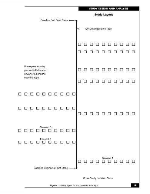
Photo plots may be permanently located anywhere along the baseline tape. Baseline End Point Stake Transect 3 Transect 2 Baseline Beginning Point Stake ∆ ∆ ∆ STUDY DESIGN AND ANALYSIS Study Layout 100-Meter Baseline Tape ∆ Figure 1. Study layout for the baseline technique. Transect 1 Study Location Stake 9
10 STUDY DESIGN AND ANALYSIS Macroplot size also depends on the size and shape of the quadrats that will be used to sample it. The sides of the macroplot should be of dimensions that are multiples of the sides of the quadrats. (1) Macroplot layout Pick one corner of the macroplot to serve as the beginning for sampling purposes. Drive an angle iron location stake into the ground at this corner. Determine the bearing of the macroplot side that will serve as the x-axis, run a tape in that direction and put an angle iron stake at the selected distance. This serves as another corner of the macroplot. Leave the x-axis tape in place for sampling purposes. Return to the origin and determine the bearing of the y-axis, which will be perpendicular to the xaxis. Run a second tape along the y-axis and put an angle iron stake in the ground at the selected distance. This serves as the third corner of the macroplot. If desired, a fourth stake may be placed at the remaining corner, but this is not necessary for sampling since sampling will be done using the two tapes serving as the x- and y-axes. See Figure 2 for an example. Leave the tapes in place until the first year’s sampling is completed. 50 m angle iron 0 m 0 m 100 m Figure 2. The two sides of a 50 m x 100 m macroplot, delineated by two tape measures. Both tapes begin with their 0 point at the beginning. Note placement of angle irons at three of the corners. Be sure to document the directions of the x- and y-axes so that the macroplot can be reconstructed if one of the angle iron stakes is missing. (2) Quadrat locations Quadrats are located in the macroplot using a coordinate system to identify the lower left-hand corner of each quadrat. (a) For example it has been determined from the pilot study that 40 samples are needed using a 1 m by 16 m quadrat. The quadrats are to be positioned so that the long side is parallel to the x-axis. On a 40 m x 80 m study site (see Figure 3), the x-axis would be the 80 m side. The total number of quadrats (N) that could be placed in that 40 m x 80 m rectangle without overlap comprises the sampled population. In this case, N is equal to 200 quadrats. (b) Along the x-axis there are 5 possible starting points (which always occur at the lower left-hand corner of each quadrat) for each 1 m x 16 m quadrat (at points 0 m, 16 m, 32 m, 48 m, and 64 m). Number these points 0 to 4 (in whole numbers) accordingly. Along the y-axis there are 40 possible starting points for each quadrat (at points 0 m, 1 m, 2 m, 3 m, 4 m, and so on until point 39 m). Number these points 0 to 39 accordingly (again in whole numbers)
- Page 1 and 2: SAMPLING VEGETATION ATTRIBUTES INTE
- Page 3 and 4: TABLE OF CONTENTS SAMPLING VEGETATI
- Page 5 and 6: TABLE OF CONTENTS TABLE OF CONTENTS
- Page 7 and 8: I. PREFACE PREFACE The intent of th
- Page 9 and 10: 2 INTRODUCTION values when individu
- Page 11 and 12: 4 INTRODUCTION represent the “pul
- Page 13 and 14: 6 INTRODUCTION G. Coordination Moni
- Page 15: 8 STUDY DESIGN AND ANALYSIS A. Plan
- Page 19 and 20: 12 STUDY DESIGN AND ANALYSIS Becaus
- Page 21 and 22: 14 STUDY DESIGN AND ANALYSIS d From
- Page 23 and 24: 16 STUDY DESIGN AND ANALYSIS b Cove
- Page 25 and 26: 18 STUDY DESIGN AND ANALYSIS sideoa
- Page 27 and 28: 4 3.5 3 2.5 20 5 STUDY DESIGN AND A
- Page 29 and 30: 22 STUDY DESIGN AND ANALYSIS C. Oth
- Page 31 and 32: 24 ATTRIBUTES Frequency is the numb
- Page 33 and 34: 26 ATTRIBUTES 2. Advantages and Lim
- Page 35 and 36: 28 ATTRIBUTES b Standing crop and p
- Page 37 and 38: 30 ATTRIBUTES
- Page 39 and 40: 32 METHODS—Photographs c Angle ir
- Page 41 and 42: METHODS—Photographs Hinge Rod sta
- Page 43 and 44: METHODS—Photographs angle iron st
- Page 45 and 46: 38 METHODS—Frequency • One tran
- Page 47 and 48: 40 METHODS—Frequency transected,
- Page 49 and 50: 42 METHODS—Frequency (3) Total fr
- Page 51: Page of Frequency 44 Study Number D
- Page 55 and 56: METHODS—Frequency The frame is ma
- Page 57 and 58: 50 METHODS—Dry Weight Rank C. Dry
- Page 59 and 60: 52 METHODS—Dry Weight Rank After
- Page 62 and 63: D. Daubenmire Method METHODS—Daub
- Page 64 and 65: METHODS—Daubenmire b Ten Cover Cl
Photo plots may be<br />
permanently located<br />
anywhere along the<br />
baseline tape.<br />
Baseline End Point Stake<br />
Transect 3<br />
Transect 2<br />
Baseline Beginning Point Stake<br />
∆<br />
∆<br />
∆<br />
STUDY DESIGN AND ANALYSIS<br />
Study Layout<br />
100-Meter Baseline Tape<br />
∆<br />
Figure 1. Study layout for the baseline technique.<br />
Transect 1<br />
Study Location Stake<br />
9


