Reverse Flow as a Possible Mechanism for Cavitation Pressure ...

Introduction 

M. Groper 

I. Etsion 

Fellow ASME 

Dept. of Mechanical Engineering, 

Technion, Haifa 32000, Israel 

In our previous paper, Groper and Etsion �1�, an attempt was 

made to understand earlier experimental observation of pressure 

build up in the cavitation zone of a submerged journal bearing. 

Two possible mechanisms were theoretically investigated �1� the 

shear of the cavity gas bubble by the lubricant film dragged 

through the cavitation, and �2� the diffusion of dissolved gas out 

of and back into the lubricant. Appropriate algorithms were developed 

and the theoretical results obtained were compared with experimental 

results reported by Etsion and Ludwig �2� and by 

Braun and Hendricks �3�. While the cavitation shape could be well 

predicted by the ‘‘shear’’ mechanism, both mechanisms, i.e., the 

‘‘shear’’ and the ‘‘diffusion’’ were incapable of predicting the experimentally 

observed pressure buildup. 

Experimental works performed by Etsion & Ludwig �2� and by 

Heshmat and Pinkus �4� revealed the existence of a reverse flow 

phenomenon towards the end of the cavitation zone. The existence 

of this reverse flow was mentioned, but its possible effects on the 

cavitation characteristics were ignored. A close examination of the 

motion picture taken by Etsion and Ludwig �2� reveals that this 

reverse flow possesses an unsteadiness pattern in time. A reverse 

flow front develops in the full film region at the cavitation end, 

penetrates the cavitation boundary and withdraws backward into 

the cavitation bubble at a relatively slow speed. It seems that this 

reverse flow adheres to the stationary bearing, while its front 

moves backward into the cavitation region. This phenomenon is 

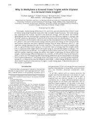
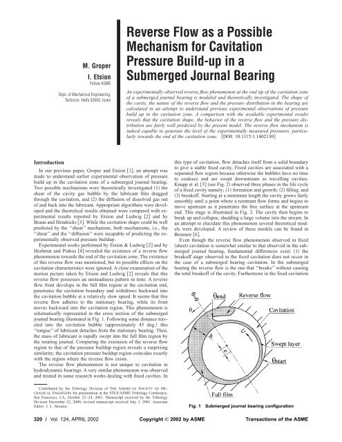
schematically represented in the cross section of the submerged 

journal bearing illustrated in Fig. 1. Following some distance traveled 

into the cavitation bubble �approximately 45 deg.� this 

‘‘tongue’’ of lubricant detaches from the stationary bearing. Then, 

the mass of lubricant is rapidly swept into the full film region by 

the rotating journal. Comparing the extension of the reverse flow 

region to that of the pressure buildup region reveals a surprising 

similarity; the cavitation pressure buildup region coincides exactly 

with the region where the reverse flow exists. 

The reverse flow phenomenon is not unique to cavitation in 

hydrodynamic bearings. A very similar phenomenon was observed 

and treated in some research works dealing with fixed cavities. In 

Reverse Flow as a Possible 

Mechanism for Cavitation 

Pressure Build-up in a 

Submerged Journal Bearing 

An experimentally observed reverse flow phenomenon at the end tip of the cavitation zone 

of a submerged journal bearing is modeled and theoretically investigated. The shape of 

the cavity, the nature of the reverse flow and the pressure distribution in the bearing are 

calculated in an attempt to understand previous experimental observations of pressure 

build up in the cavitation zone. A comparison with the available experimental results 

reveals that the cavitation shape, the behavior of the reverse flow and the pressure distribution 

are fairly well predicted by the present model. The reverse flow mechanism is 

indeed capable to generate the level of the experimentally measured pressures, particularly 

towards the end of the cavitation zone. �DOI: 10.1115/1.1402130� 

this type of cavitation, flow detaches itself from a solid boundary 

to give a stable fixed cavity. Fixed cavities are associated with a 

separated flow region because otherwise the bubbles have no time 

to coalesce and are swept downstream as travelling cavities. 

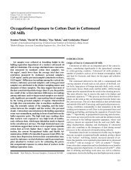
Knapp et al. �5� �see Fig. 2� observed three phases in the life cycle 

of a fixed cavity namely; �1� formation and growth; �2� filling; and 

�3� breakoff. Starting at a minimum length the cavity grows fairly 

smoothly until a point where a reentrant flow forms and begins to 

move upstream as it penetrates the free surface at the upstream 

end. This stage is illustrated in Fig. 2. The cavity then begins to 

break up and collapse, shedding a large volume into the stream. In 

an attempt to elucidate this phenomenon several theoretical models 

were developed. A review of these models can be found in 

Brennen �6�. 

Even though the reverse flow phenomenon observed in fixed 

�sheet� cavitation is somewhat similar to that observed in the submerged 

journal bearing, fundamental differences exist; �1� the 

breakoff stage observed in the fixed cavitation does not occur in 

the case of a submerged bearing cavitation. In the submerged 

bearing the reverse flow is the one that ‘‘breaks’’ without causing 

the total breakoff of the cavity. Furthermore in the fixed cavitation 

Contributed by the Tribology Division of THE AMERICAN SOCIETY OF ME- 

CHANICAL ENGINEERS for presentation at the STLE/ASME Tribology Conference, 

San Francisco, CA, October 22–24, 2001. Manuscript received by the Tribology 

Division December 22, 2000; revised manuscript received July 3, 2001. Associate 

Editor: J. L. Streator. Fig. 1 Submerged journal bearing configuration 

320 Õ Vol. 124, APRIL 2002 Copyright © 2002 by ASME Transactions of the ASME

Fig. 2 Penetration of the reentrant jet into a fixed cavity „schematic… 

„Ref. †5‡… 

case, cavity breakoff occurs when the reentrant flow completely 

separates the cavitation bubble from the stationary surface. Contrary, 

in the submerged bearing cavitation the reentrant flow collapses 

much before reaching the cavitation start region. This finding 

may indicate that some kind of film flow instability is 

involved, causing the collapse of the reverse flow ‘‘tongue.’’ �2� In 

the film reformation zone of the submerged bearing a positive 

pressure gradient exists. This pressure gradient leads to a reverse 

Poiseuille flow, graphically presented by Coyne and Elrod �7� and 

Pan �8�. This pressure gradient does not necessarily exist in the 

fixed cavitation case. Finally, the reverse flow region in the submerged 

bearing obeys the creeping flow conditions and the hydrodynamic 

theory assumptions while the reentrant flow in fixed 

cavitations comply with the assumptions of the potential flow 

theory. 

In the present paper an attempt is made to develop the necessary 

model and allow a theoretical investigation of the nature and 

behavior of the reverse flow and its possible effect on the pressure 

build up in the cavitation zone of a submerged journal bearing. 

Theory 

Figure 3 illustrates a cross section of a submerged journal bearing 

in the film reformation region of the cavitation zone. At t 

�t 0 a front having a height hb0 and a velocity profile ub0 begins 

to withdraw upstream penetrating into the cavitation region. As 

the flow moves backward its profile develops and at t�t 1 it 

reaches a height hb and its velocity profile is ub . The velocity of 

the lubricant at the liquid/gas interface is Ub . This ‘‘tongue’’ of 

lubricant at its interface between the liquid and the gas possess a 

deformable boundary. This type of boundary can display a waviness 

pattern and if subjected to certain conditions its waviness 

may grow and even become unstable �see Ref. �9��. 

The usual assumptions of the hydrodynamic theory are applied 

to the gas and the liquid phases, i.e., negligible inertia, film height 

small compared with the other dimensions, etc. It is also assumed 

that the reverse flow is two dimensional with no spreading of 

liquid in the z direction. This assumption is based on observations 

from the experimental findings of Etsion and Ludwig �2� and is 

commonly used in the treatment of reverse flow in fixed cavitations, 

for example Brennen �6�. In the experimental work of Etsion 

and Ludwig �2� it was clearly observed that the reverse flow 

velocity is much slower than the journal velocity. So, for the treatment 

of the reverse flow a quasi steady state assumption is made. 

For the purpose of calculating the pressure in the cavitation region 

the possible waviness of the liquid/gas interface is ignored and 

calculations are made assuming a nominal average height of the 

reverse flow denoted by h b . 

Consider a control volume of unit axial length and a circumferential 

length R�� with a height corresponding to the thickness of 

the reverse flow, as is shown in Fig. 4. We shall consider the 

momentum equation in the angular �� direction for this control 

volume in the case of a steady flow. The force in the �� direction 

is given by 

dF �� P cav� dP cav 

Rd� R�� h b�dh b��P cavh b�� 

P cav 

� dP cav 

2Rd� R�� dh b�� wR��, (1) 

where � w is the shear stress at the stationary bearing wall, and 

P cav denotes the local cavitation pressure. 

Based on the assumptions of the hydrodynamic theory, inertia 

terms can be neglected. Then, canceling terms and dropping second 

order expressions, we get 

or 

dPcav � hb Rd� �� w� Rd��0 (2) 

�� w�h b 

Fig. 3 Model for the reverse flow in the film reformation region 

Fig. 4 The forces acting on a control volume in the reverse 

flow 

dPcav . (3) 

Rd� 

Journal of Tribology APRIL 2002, Vol. 124 Õ 321

Using Newton’s viscosity law to replace � w , 

�u b 

�w�� l � , (4) 

�y 

y�h 

and substituting in Eq. �3�, the momentum equation in the angular 

direction for the control volume in Fig. 4 is given by 

�u b 

�� l � �h b 

�y 

y�h 

dPcav . (5) 

Rd� 

At this stage, following the well known integral-momentum 

method, a velocity profile should be assumed. Based on the large 

viscosity difference between the gas and the lubricant, for the 

purpose of this analysis, one can assume that the reverse flow at 

the interface is almost not affected by the shear with the gas 

phase. So, the velocity profile of the reverse flow will be assumed 

as a second-degree polynom of the form 

ub�a ��b ��y�c ��y 2 . (6) 

The usual assumptions of no slip at the solid boundaries and no 

shear stress at the interface are given by 

u b�h��0 

�u b��h�h 

�y 

b� �0. (7) 

Based on the ‘‘no spreading in the z direction’’ assumption, the 

continuity of mass flow for any section of the reverse flow is 

given by 

h 

Fig. 5 Boundary of the cavity—schematic description 

�R�y�h ��end�� ul��end�� h��end� � 3�h �� end��2h ��y 

2 �1� . (14) 

h��end� �h�h 

ubdy�const.�M, (8) 

b 

where M express the mass flow per unit axial length of the reverse 

flow. 

Substituting the expressions from Eq. �7� and Eq. �8� in the 

velocity profile given in Eq. �6� the a, b, and c coefficients can be 

calculated, namely, 

a�� 3 Mh�2h a�h� 

2 ��h b� 3 b��3 Mha ��h b� 3 c�� 3 M 

2 ��h b� 3 . 

(9) 

Going back to Eq. �5� and replacing the velocity ub with the 

velocity profile in Eq. �6� and the coefficients in Eq. �9�, an equation 

for the pressure gradient dPcav /d� in the cavity is obtained: 

dPcav d� � 3� lRM 

3 , (10) 

hb where hb�h b(�). 

The constant M can be calculated using a flow rate balance at 

the cavity tip (�� end). �See the schematic description of the 

cavity boundary as shown in Fig. 5�. This flow balance is given by 

3 

h��end� �P �Rh��end� �Rh�� . (11) 

12�l R�� 2 

�end 

Making use of the expression in Eq. �11� the pressure gradient 

�P/�� at �� end is obtained: 

�P 

� �� end 

6� l�R 2 

2 

h � ��end� 1� 2h � 

. (12) 

h��end�� The lubricant velocity profile at the cavity tip (�� end) is composed 

of a Couette and a Poiseuille term: 

ul��end�� 1 

The solution of Eq. �14� for ul(�end )�0 in the domain 0�y 

�h (�end ) results in zero lubricant velocity at two locations. One at 

y�h (�end ) , to satisfy the no slip condition at the ‘‘wall.’’ The 

second at 

2 

h��end� y 0� 

. (15) 

3�h ��end��2h �� 

Then the constant M �see Eq. 8� is given by 

h��end� M��y 

ul��end�dy� 0 

�P 

h��end��y y�y�h ��end 

2� l R�� R. (13) 

h 

�end 

��end� The pressure gradient obtained in Eq. �12� can be substituted in 

Eq. �13� to give the lubricant velocity profile at the cavity end: 

4 �R�h ��end��3h �� 

27 

3 

�h ��end��2h �� 2 . (16) 

For the calculation of the pressure in the cavity, a similar approach 

to the one used in our previous paper, Groper and Etsion 

�1� shall be used. One obtains 

dPcav d� � 6� gR��R�U b� 

2 , (17) 

hg where Ub is the velocity of the reverse flow at the gas/liquid 

interface �see Fig. 3� and hg is the thickness of the gas film given 

by hg�h�h b�h � . This velocity is calculated using the velocity 

profile of the reverse flow from Eq. �6� with the coefficients given 

in Eq. �9�: 

Ub�u b�y�h�hb �� 3 M 

. (18) 

2 hb Making use of this expression in Eq. �17� a more detailed expression 

for the cavity pressure gradient is obtained: 

dPcav d� � 

6� gR� �R� 3M 

2h b� 

2 . (19) 

hg The boundary condition for the solution of this differential 

equation is given by �see Groper and Etsion, �1�� 

Pcav��start��P sat . (20) 

322 Õ Vol. 124, APRIL 2002 Transactions of the ASME

Substituting the expression given in Eq. �19� for the pressure 

gradient dP cav /d� into Eq. �10� an expression for the reverse flow 

thickness, h b can be obtained: 

� 2 g 2 

Mhg� hb�2�Rhb�3M �. (21) 

�l The dimensionless form of the this equation is 

2 2 

M¯h¯ 

g��¯h¯ b�2h¯ b�3M¯�, (22) 

where the dimensionless expressions are given by 

h¯ b� h b 

C 

M 

M¯� . (23) 

�RC 

The dimensionless form of the differential Eq. �19� for the cavity 

pressure gradient dP¯ cav /d� is given by 

dP¯ cav 

d� ��¯� 1�Ū b 

h¯ g 2 � 

, (24) 

where the dimensionless 

b�� 

velocity at the interface Ūb is given by 

0 h¯ 

b�0 

Ū 

� 3M¯ . (25) 

h¯ 

b�0 

2h¯ 

b 

Substituting the expression for M from Eq. �16� �in its dimensionless 

form� into the expression for Ū b �Eq. 25�, 

Ū b�� 

� 2 

9 

0 h¯ b�0 

�h¯ ��end ��3h �� 3 

�h¯ ��end ��2h¯ �� 2 h¯ b 

. (26) 

h¯ 

b�0 

The dimensionless form of the boundary condition �20� is 

P¯ cav��start ��P¯ sat�0. (27) 

Equation �22� describes the development of the reverse flow 

thickness as it withdraws backward into the cavity. The differential 

Eq. �24� subject to the boundary condition �27� describes the 

pressure field in the cavity, under the influence of the reverse flow. 

The reverse flow starts in the full film region at the cavity tip, 

penetrates the cavity boundary and develops a ‘‘tongue’’ shape 

while retreating into the cavity. When this ‘‘tongue’’ reaches a 

specific length it collapses. Based on the moving picture taken by 

Etsion and Ludwig �2�, the collapse of the reverse flow occurs 

abruptly. It seems that this collapse is caused by a momentary 

contact of the reverse flow and the lubricant layer swept by the 

rotating shaft. 

Based on the developed theory, the reverse flow thickness and 

the cavity pressure for the submerged bearing in Ref. �2� ware 

calculated. It was found that in order for a contact between the 

reverse flow and the lubricant layer swept by the rotating shaft to 

happen, the reverse flow ‘‘tongue’’ must penetrate much deeper 

into the cavity region than the 30–45 deg. observed in Ref. �2�. 

This finding might suggest that some instability mechanism developed 

on the gas/liquid interfaces, caused it to became wavy and 

develop a momentary local increase in thickness. Then, contact 

between the reverse flow interface and the lubricant layer swept 

by the rotating shaft may become possible much before the location 

obtained using the theory developed. 

Kelvin-Helmholtz instability occurs when there is a shear motion 

of two fluids flowing along each other. A common method for 

the determination of the flow stability is by the observation of the 

interface waviness amplitude following an excitation applied at 

this interface. Linear analysis permits to calculate the critical excitation 

wavelength. An excitation with a shorter than critical 

Fig. 6 The reverse flow and the gas layer thickness 

wavelength will decay in time while an excitation with a longer 

than critical wavelength will evolve. In this case, linear analysis as 

performed by Yih �9� leads to an unbounded increase in the amplitude 

of the interface waviness. 

Hooper and Grimshaw �10� and Oron and Rosenau �11� present 

a nonlinear analysis of a perturbed interface that separates two 

superposed viscous fluid layers. This analysis permits the calculation 

of the finite amplitude for the perturbed interface following 

its excitation by a longer than critical wavelength perturbation. 

The configuration of the flow in the works of Hooper and Grimshaw 

�10� and Oron and Rosenau �11� was based on two superposed 

fluids of different viscosity flowing in a channel of an infinite 

length. Initially the interface separating the two fluids was 

perturbed and the evolution of this perturbation in time was studied. 

It was shown that the interface returns to its original undisturbed 

state when applying a perturbation having a wavelength 

shorter than the critical one but evolve to some finite and steady 

amplitude for the case where the perturbation wavelength was 

longer than the critical one. 

The reverse flow studied in this work does not have an infinite 

length as in Hooper and Grimshaw �10� and Oron and Rosenau 

�11�. At any given moment t�t 0 the momentary length of the 

reverse flow is l. As such, the perturbation wavelength applied at 

the interface can not be longer than l. Therefore, when the length 

of the reverse flow, l, is shorter than the critical wavelength, l cr , 

the flow is perfectly stable, any disturbance will decay and the 

reverse flow thickness will remain h¯ b as calculated using Eq. �21�. 

Starting at a certain moment, the length of the reverse flow becomes 

longer than the critical wavelength, l cr . For this case the 

interface will evolve to some finite and steady state amplitude. At 

this stage, the total thickness of the reverse flow is composed of 

two components: �1� h¯ b as calculated using equation �21�, and �2� 

the amplitude of the disturbance. As long as the total thickness 

does not cause the reverse flow to contact the swept flow on the 

rotating journal �see Fig. 6�, nothing happens and the reverse flow 

continues its withdrawal into the cavitation bubble. The reverse 

flow will continue and withdraw until its length will reach a specific 

length, l b �see Fig. 6�. At this explicit length, disturbance 

waves having a wavelength equal to l b will cause the interface to 

evolve and eventually contact the swept lubricant layer. The momentary 

contact will cause the collapse of the reverse flow into 

the swept lubricant layer. The mass of lubricant of the reverse 

flow ‘‘tongue’’ will be carried away toward the cavitation tip, into 

the full film region, and a new reverse flow cycle will commence. 

The nonlinear analysis performed here for the interface evolution 

of two superposed fluids is based on the works of Hooper and 

Grimshaw �10� and Oron and Rosenau �11� for the Poiseuille case. 

This flow is known to be unstable for a long wavelength disturbance 

which persists at arbitrary small values of Reynolds number 

�Yih �9��. 

The thickness of the lower fluid �the gas� is given by h g , its 

viscosity by � g , � g is the density, and u g(y) is the velocity field 

in the gas. The upper fluid �the reverse flow� thickness is h b , its 

viscosity is � l , � l is the density and the velocity field is given by 

u b(y). A coordinate system x�y� �see Fig. 6� is located at the 


interface. The interface is disturbed from its initial state at y� 

�0 toy��(x�,t). The dimensionless expressions are given by 

m� � l 

� g 

r� � l 

� g 

n� h b 

h g 

t¯� tU b 

h g 

x¯�� x� 

h g 

y¯�� y� 

. (28) 

hg Identically to Hooper and Grimshaw �10� we assume that the interfacial 

disturbance is small, therefore, 

�¯�� sA��,��, (29) 

where �s is s small perturbation parameter, � is the stretched coordinate 

in the x¯� direction and � is the stretched time coordinate. 

Using this notation and following Hooper and Grimshaw �10� 

development, the Kuramoto-Sivashinsky, �K-S�, equation for the 

amplitude of the interfacial disturbance is obtained: 

�A �A 

��A 

�� 2A ��2 �� 4A ��4 �0. (30) 

The equations for the calculations of the constants �, �, and � are 

given by Oron and Rosenau �11�. These constant values depend 

upon the viscosity, density and thickness ratio. � is identified with 

the growth rate of the linear stability analysis, � is identified with 

the stabilization effect of the surface tension and � expresses the 

strength of the nonlinear effect. 

Several methods exist for the solution of this non-linear, partial 

differential equation. For the scope of this work the equation was 

solved using an implicit, Crank-Nicolson, finite difference 

scheme. The solution domain is 0�� l¯. The relation between 

the stretched length, l¯ and the physical length, l is given by 

l¯� l 

�s . (31) 

hg The interface initial excitation is introduced by the initial condition 

A��,0��C 1 cos N1��C 2 sin N2�, (32) 

where C1 and C2 are constants and N1 and N2 are integers. 

Two possibilities exist for the collapse of the reverse flow 

‘‘tongue’’: �1� a momentary contact of the reverse flow with the 

swept lubricant layer, and �2� a disturbance with an amplitude hb causing the separation of the reverse flow from the bearing �the 

‘‘wall’’�. For case �1� the collapse of the reverse flow will occur 

when 

��h g . (33) 

While for case �2�, this will happen when 

��h b . (34) 

The physical amplitude of the disturbed interface, �, is given by 

��¯h g . Then, making use of Eq. �29�, Eq. �33�, and Eq. �34� the 

following conditions for the collapse of the reverse flow are obtained. 

For Case „1…. 

�sA�1. (35) 

For Case „2…. 

�sA�n. (36) 

The length of the reverse flow prior to its collapse is given by 

lbf� l¯ 

bh g 

�U 

� 

b�t. (37) 

s 

This length is composed of two expressions. The first expression 

is the physical length of the reverse flow that permits the 

development of a disturbance with a wavelength long enough to 

cause the collapse. From this moment an additional time, �t will 

pass until the disturbed amplitude of the interface will evolve 

causing the collapse of the reverse flow. The second expression in 

Eq. �37� describes the additional length the reverse flow travels in 

the time interval �t. 

The computation method for the pressure field in the full film 

region as well as for the cavity shape is similar here to the one 

developed and presented in our previous paper �Groper and Etsion, 

�1��. The major difference is the incorporation of the reverse 

flow and the instability mechanism. For the numerical calculations 

purpose a marching procedure was introduced. The withdrawal 

process of the reverse flow begins at the angular location � end with 

a withdraw step ��. For each step, the reverse flow thickness and 

the local cavity pressure are calculated. In addition, at each step, 

starting at the angular location where the length of the reverse 

flow ‘‘tongue’’ exceeds the critical length l¯ cr , the interface is 

disturbed and the amplitude of the disturbed interface is calculated. 

Then, the fulfillment of each of the collapse conditions as 

described by Eq. �35� and Eq. �36� is verified. If none of the 

conditions is fulfilled, an additional withdraw step �� is performed 

and the calculation process is repeated. This process continues 

until the angular location where the development of amplitude 

large enough to cause collapse is possible. From this moment 

an additional time, �t will pass until the disturbed amplitude of 

the interface will evolve causing the collapse of the reverse flow. 

Results and Discussion 

The submerged hydrodynamic bearing tested by Etsion and 

Ludwig �2� was selected in the present analysis to evaluate the 

proposed mechanism for the pressure build up in the cavitation 

region. The various geometrical and operational parameters are 

summarized in Table 1. The suggested model, i.e., the ‘‘reverse 

flow’’ model was analyzed and the results were compared with the 

experimental ones described by Etsion and Ludwig �2�. 

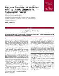
Figure 7 presents a comparison between the calculated and the 

experimental cavity pressure distribution along the cavity center at 

z�0 for two values of supply pressure, 154.4 kPa and 127.2 kPa. 

As can be seen the theoretical and experimental results for the 

cavity pressure field show a reasonable good correlation. Particularly, 

the phenomenon of pressure buildup towards the cavity end, 

that was experimentally observed by Etsion and Ludwig �2� is 

well predicted by the model developed here. In addition, the predicted 

cavity start angle, �start , as well as the predicted cavity end 

angle, �end show a reasonable good correlation with the experimental 

results. 

Similar results were obtained for other operation conditions described 

in Refs. �2� and �3�, namely, good correlation for the cavity 

boundary and for the pressure distribution inside the cavitation 

Table 1 Geometrical data, operation conditions, and lubricant 

properties 


Fig. 7 Predicted versus measured „Ref. †2‡… cavity pressure field at the bearing center 

zone. Hence, the discussion above is not limited to the results 

presented in Fig. 7 but can be considered as representative of the 

general behavior of submerged journal bearings. 

Conclusion 

A reverse flow phenomenon that was observed in previous experiments 

at the end of the cavitation zone in a submerged journal 

bearing was modeled and analyzed. This was done in an attempt 

to understand the mechanism for pressure build up in the cavitation 

zone that was measured in these previous experiments. 

An appropriate algorithm that allows the calculation of the 

cavitation shape, the penetration of the reverse flow into the cavitation 

zone and the pressure distribution inside the cavitation zone 

of a submerged journal bearing was developed. 

The theoretical results obtained from the model were compared 

with published results of the previous experiments. Very good 

correlation with the experimental results was obtained by adopting 

a Kelvin-Helmholtz instability model that explains the observed 

instability of the reverse flow. 

It was found that the pressure field throughout the cavity and 

particularly the pressure buildup towards the cavity end could be 

fairly well predicted by the reverse flow mechanism. 

Nomenclature 

A � dimensionless, stretched amplitude of the disturbed 

interface, �¯�� sA(�,�) 

C � radial clearance 

D � bearing diameter 

e � bearing eccentricity 

h � local clearance, C(1�� cos �) 

h¯ � dimensionless local clearance, h/C 

h� � asymptotic thickness of the swept lubricant layer 

hb � thickness of the reverse flow 

l � momentary length of the reverse flow 

lb � reverse flow length capable of causing the collapse of 

the reverse flow 

lbf � momentary length of the reverse flow at the collapse 

moment, R(� end�� b) 

l¯ � dimensionless, stretched momentary length of the 

reverse flow, l¯�l/h g•� s 

l¯ cr � dimensionless, stretched critical length of the reverse 

flow, l¯ cr�2�•��/� 

M � mass flow per unit thickness of the reverse flow 

M¯ � dimensionless mass flow per unit thickness of the 

reverse flow, M¯�M/�RC 

P � pressure 

P¯ � dimensionless pressure, (P�P sat)/P sat� 

R � bearing radius 

t � time 

u � fluid velocity in circumferential direction 

u b � velocity of the reverse flow 

u l � lubricant velocity in the full film region 

U b � velocity of the reverse flow at the interface in the x 

direction 

Ū b � dimensionless velocity of the reverse flow at the interface, 

Ū b�U b /�R 

x,y,z � coordinates system 

x�,y� � coordinate system located at the interface �Fig. 6� 

y¯ � dimensionless coordinate, y/C 

z¯ � dimensionless coordinate, 2z/L 

� � dimensionless eccentricity, e/C 

� s � small perturbation parameter 

� � bearing width over diameter ratio, L/2R 

� � viscosity 

�¯ � viscosity ratio, � g /� l 

� � stretched coordinate in the x¯� direction 

� � location of the disturbed interface 

� � angular coordinate 

� b � angular location of the reverse flow collapse 

� start � angular location of the cavity start 

� end � angular location of the cavity end 

� � dimensionless, stretched time, �� s 2 •tUb /h g 

� � angular speed of journal 

� � bearing number, 6� l�/P sat•(R/C) 2 

Subscripts 

0 � at the start location of the reverse flow, (� end) 

b � reverse 

cav � cavity 

end � cavity end 

g � gas 


l � liquid 

sat � saturation 

start � start of the cavitation zone 

sup � supply �pressure� 

References 

�1� Groper, M., and Etsion, I., 2001, ‘‘The Effect of Shear Flow and Dissolved 

Gas Diffusion on the Cavitation in a Submerged Journal Bearing,’’ ASME J. of 

Tribol., 123, pp. 494–500. 

�2� Etsion, I., and Ludwig, L. P., 1982, ‘‘Observation of Pressure Variation in the 

Cavitation Region of Submerged Journal Bearings,’’ ASME J. Lubr. Technol., 

104, pp. 157–163. 

�3� Braun, M. J., and Hendricks, R. C., 1984, ‘‘An Experimental Investigation of 

the Vaporous/Gaseous Cavity Characteristics of an Eccentric Journal Bearing,’’ 

STLE Tribol. Trans., 27, No. 1, pp. 1–14. 

�4� Heshmat, H., and Pinkus, O., 1985, ‘‘Performance of Starved Journal Bearings 

With Oil Ring Lubrication,’’ ASME J. Tribol., 107, pp. 23–32. 

�5� Knapp, R. T., Daily, J. W., and Hammit, F. G., 1970, Cavitation, McGraw-Hill, 

New-York. 

�6� Brennen, C. E., 1995, Cavitation and Bubble Dynamics, Oxford University 

Press, New York. 

�7� Coyne, J. C., and Elrod, H. G., 1971, ‘‘Conditions for the Rupture of a Lubricating 

Film, Part 2: New Boundary Conditions for Reynolds’ Equation,’’ 

ASME J. Lubr. Technol., 93, pp. 156–167. 

�8� Pan, C. H. T., 1980, ‘‘An Improved Short Bearing Analysis for the Submerged 

Operation of Plain Journal Bearings and Squeeze-Film Dampers,’’ ASME J. 

Lubr. Technol., 102, pp. 320–332. 

�9� Yih, C. S., 1967, ‘‘Stability of Parallel Laminar Flow With a Free Surface,’’ J. 

Fluid Mech., 27, pp. 337–352. 

�10� Hooper, A. P., and Grimshaw, R., 1985, ‘‘Nonlinear Instability at the Interface 

Between Two Viscous Fluids,’’ Phys. Fluids, 28, No. 1, pp. 37–45. 

�11� Oron, A, and Rosenau, P., 1989, ‘‘Nonlinear Evolution and Breaking of Interfacial, 

Rayleigh-Taylon Waves,’’ Phys. Fluids A, A1, pp. 1155–1165.

Reverse Flow as a Possible Mechanism for Cavitation Pressure ...

Create successful ePaper yourself

Delete template?

Save as template?