Simulation of electric and magnetic fields using FEMM - FH Aachen ...

More documents

Recommendations

Info

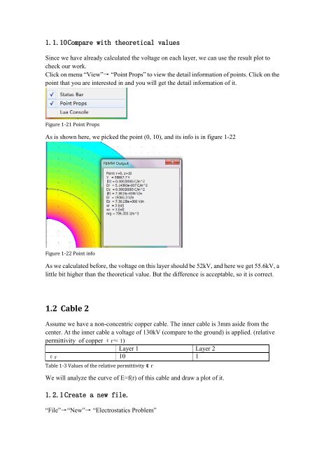
1.1.10 Compare with theoretical values Since we have already calculated the voltage on each layer, we can use the result plot to check our work. Click on menu “View”→ “Point Props” to view the detail information of points. Click on the point that you are interested in and you will get the detail information of it. Figure 1-21 Point Props As is shown here, we picked the point (0, 10), and its info is in figure 1-22 Figure 1-22 Point info As we calculated before, the voltage on this layer should be 52kV, and here we get 55.6kV, a little bit higher than the theoretical value. But the difference is acceptable, so it is correct. 1.2 Cable 2 Assume we have a non-concentric copper cable. The inner cable is 3mm aside from the center. At the inner cable a voltage of 130kV (compare to the ground) is applied. (relative permittivity of copper εr≈ 1) Layer 1 Layer 2 εr 10 1 Table 1-3 Values of the relative permittivityεr We will analyze the curve of E=f(r) of this cable and draw a plot of it. 1.2.1 Create a new file. “File”→“New”→ “Electrostatics Problem”
1.2.2 Set problem definition. Press Menu: “Problem”. Figure 1-23 Problem definition dialogue box 1.2.3 Create a new model To draw a set of non-concentric circles, first we need to have three concentric circles using function ”Operate on arc Segments”. First we should mark some nodes using “Operate on nodes”, then we switch to function . Select 2 nodes one by another to draw an arc segments in between, and then we will have half of the circle. Now we need the other half so we select these 2 nodes again but this time change the selection order. In this way, we will be able to make all three circles. Figure 1-24 New model step 1 Our model is a non-concentric cable, so we shift the inner circle, using ”Move/Remote the selected Object”. First switch to function and select the inner circle. Press , shift it along X-axis for 3 units.
Page 1 and 2: Simulation of electric and magnetic
Page 3 and 4: Acknowledgments I would like to exp
Page 5 and 6: 1.4.1 Create a new file. ..........
Page 7 and 8: 3.2.1 Create new file .............
Page 9 and 10: Current flow procedures: 1. Create
Page 11 and 12: Problem Type: Axisymmetric Length U
Page 13 and 14: Figure 1-7 Voltage on layer 1 Groun
Page 15 and 16: 1.1.7 Generate mesh and run FEA Run
Page 17: Figure 1-18E,t plot And this plot c
Page 21 and 22: But here we have a non-symmetric ca
Page 23 and 24: 1.2.6 Define conductor and material
Page 25 and 26: Figure 1-38 Contour Then select E,
Page 27 and 28: 1.3.3 Create a new model We treat t
Page 29 and 30: 1.3.5 Set up the properties of mate
Page 31 and 32: Figure 1-53 Result 1.3.9 Plot field
Page 33 and 34: Inner cable 2*ri=10 mm Flange(Flans
Page 35 and 36: Figure 1-62 Conductor properties Fi
Page 37 and 38: Figure 1-67Contour Use function to
Page 39 and 40: 1.5.2 Set problem definition. Press
Page 41 and 42: 1.5.6 Define conductor properties T
Page 43 and 44: Figure 1-83D,t plot 1.5.11 Comparis
Page 45 and 46: And this time it seems to be smooth
Page 47 and 48: The outer shell is connected with g
Page 49 and 50: 1.6.8 Plot field values Draw E and
Page 51 and 52: 1.7.3 Create a new model Draw 3 seg
Page 53 and 54: 1.7.8 Display results Figure 1-111R
Page 55 and 56: 2. Electrical Field Before we deal
Page 57 and 58: 2.1.5 Define conductor properties S
Page 59 and 60: Draw the contour from (0, 0) to (14
Page 61 and 62: Figure 2-13 New model step 2 2.2.4
Page 63 and 64: σr=1 for schicht2 Figure 2-19Prope
Page 65 and 66: 2.2.9 Plot field values Choose cont
Page 67 and 68: Figure 3-2 Problem definition 3.1.3
Page 69 and 70:
3.1.7 Define circuits. Select menu
Page 71 and 72:
3.1.10 Associate Properties with bo
Page 73 and 74:
Click on button . Then in the dialo
Page 75 and 76:
3.2 Air gap Here we have a square c
Page 77 and 78:
Figure 3-24 Circuit 3.2.8 Place Blo
Page 79 and 80:
Figure 3-29 Mesh 3.2.12 Analysis re
Page 81 and 82:
3.2.13 Plot Field Values Draw conto
Page 83 and 84:
List of figures Figure 1-1 Create a
Page 85 and 86:
Figure 1-89 New model .............
Page 87:
List of tables Table 1-1 Values of
show all

Simulation of electric and magnetic fields using FEMM - FH Aachen ...

You also want an ePaper? Increase the reach of your titles

Delete template?

Save as template?