3D graphics eBook - Course Materials Repository
3D graphics eBook - Course Materials Repository
3D graphics eBook - Course Materials Repository

Create successful ePaper yourself
Turn your PDF publications into a flip-book with our unique Google optimized e-Paper software.
Radiosity 140<br />
Overview of the radiosity algorithm<br />
The surfaces of the scene to be rendered are each divided up into one or more smaller surfaces (patches). A view<br />
factor is computed for each pair of patches. View factors (also known as form factors) are coefficients describing<br />
how well the patches can see each other. Patches that are far away from each other, or oriented at oblique angles<br />
relative to one another, will have smaller view factors. If other patches are in the way, the view factor will be<br />
reduced or zero, depending on whether the occlusion is partial or total.<br />
The view factors are used as coefficients in a linearized form of the rendering equation, which yields a linear system<br />
of equations. Solving this system yields the radiosity, or brightness, of each patch, taking into account diffuse<br />
interreflections and soft shadows.<br />
Progressive radiosity solves the system iteratively in such a way that after each iteration we have intermediate<br />
radiosity values for the patch. These intermediate values correspond to bounce levels. That is, after one iteration, we<br />
know how the scene looks after one light bounce, after two passes, two bounces, and so forth. Progressive radiosity<br />
is useful for getting an interactive preview of the scene. Also, the user can stop the iterations once the image looks<br />
good enough, rather than wait for the computation to numerically converge.<br />
Another common method for solving<br />
the radiosity equation is "shooting<br />
radiosity," which iteratively solves the<br />
radiosity equation by "shooting" light<br />
from the patch with the most error at<br />
each step. After the first pass, only<br />
those patches which are in direct line<br />
of sight of a light-emitting patch will<br />
As the algorithm iterates, light can be seen to flow into the scene, as multiple bounces are<br />
computed. Individual patches are visible as squares on the walls and floor.<br />
be illuminated. After the second pass, more patches will become illuminated as the light begins to bounce around the<br />
scene. The scene continues to grow brighter and eventually reaches a steady state.<br />
Mathematical formulation<br />
The basic radiosity method has its basis in the theory of thermal radiation, since radiosity relies on computing the<br />
amount of light energy transferred among surfaces. In order to simplify computations, the method assumes that all<br />
scattering is perfectly diffuse. Surfaces are typically discretized into quadrilateral or triangular elements over which a<br />
piecewise polynomial function is defined.<br />
After this breakdown, the amount of light energy transfer can be computed by using the known reflectivity of the<br />
reflecting patch, combined with the view factor of the two patches. This dimensionless quantity is computed from<br />
the geometric orientation of two patches, and can be thought of as the fraction of the total possible emitting area of<br />
the first patch which is covered by the second patch.<br />
More correctly, radiosity B is the energy per unit area leaving the patch surface per discrete time interval and is the<br />
combination of emitted and reflected energy:<br />
where:<br />
• B(x) i dA i is the total energy leaving a small area dA i around a point x.<br />
• E(x) i dA i is the emitted energy.<br />
• ρ(x) is the reflectivity of the point, giving reflected energy per unit area by multiplying by the incident energy per<br />
unit area (the total energy which arrives from other patches).<br />
• S denotes that the integration variable x' runs over all the surfaces in the scene<br />
• r is the distance between x and x'