3D graphics eBook - Course Materials Repository

3D Rendering
PDF generated using the open source mwlib toolkit. See http://code.pediapress.com/ for more information.
PDF generated at: Tue, 11 Oct 2011 09:36:28 UTC

Contents
Articles
Preface 1
3D rendering 1
Concepts 5
Alpha mapping 5
Ambient occlusion 5
Anisotropic filtering 8
Back-face culling 11
Beam tracing 12
Bidirectional texture function 13
Bilinear filtering 13
Binary space partitioning 15
Bounding interval hierarchy 20
Bounding volume 23
Bump mapping 26
Catmull–Clark subdivision surface 28
Conversion between quaternions and Euler angles 30
Cube mapping 33
Diffuse reflection 36
Displacement mapping 39
Doo–Sabin subdivision surface 41
Edge loop 42
Euler operator 43
False radiosity 44
Fragment 45
Geometry pipelines 46
Geometry processing 47
Global illumination 47
Gouraud shading 50
Graphics pipeline 52
Hidden line removal 54
Hidden surface determination 55
High dynamic range rendering 58

Image-based lighting 64
Image plane 65
Irregular Z-buffer 65
Isosurface 66
Lambert's cosine law 67
Lambertian reflectance 70
Level of detail 71
Mipmap 74
Newell's algorithm 76
Non-uniform rational B-spline 77
Normal mapping 85
Oren–Nayar reflectance model 88
Painter's algorithm 91
Parallax mapping 93
Particle system 94
Path tracing 97
Per-pixel lighting 101
Phong reflection model 101
Phong shading 105
Photon mapping 106
Photon tracing 109
Polygon 111
Potentially visible set 111
Precomputed Radiance Transfer 114
Procedural generation 115
Procedural texture 121
3D projection 124
Quaternions and spatial rotation 127
Radiosity 138
Ray casting 145
Ray tracing 147
Reflection 154
Reflection mapping 156
Relief mapping 159
Render Output unit 160
Rendering 160
Retained mode 170
Scanline rendering 170

Schlick's approximation 173
Screen Space Ambient Occlusion 173
Self-shadowing 177
Shadow mapping 177
Shadow volume 183
Silhouette edge 188
Spectral rendering 189
Specular highlight 190
Specularity 193
Sphere mapping 194
Stencil buffer 195
Stencil codes 196
Subdivision surface 200
Subsurface scattering 204
Surface caching 206
Surface normal 207
Texel 210
Texture atlas 211
Texture filtering 212
Texture mapping 214
Texture synthesis 217
Tiled rendering 222
UV mapping 223
UVW mapping 225
Vertex 225
Vertex Buffer Object 227
Vertex normal 232
Viewing frustum 233
Virtual actor 234
Volume rendering 237
Volumetric lighting 243
Voxel 244
Z-buffering 248
Z-fighting 252
Appendix 254
3D computer graphics software 254

References
Article Sources and Contributors 261
Image Sources, Licenses and Contributors 266
Article Licenses
License 269

3D rendering
Preface
3D rendering is the 3D computer graphics process of automatically converting 3D wire frame models into 2D
images with 3D photorealistic effects on a computer.
Rendering methods
Rendering is the final process of creating the actual 2D image or animation from the prepared scene. This can be
compared to taking a photo or filming the scene after the setup is finished in real life. Several different, and often
specialized, rendering methods have been developed. These range from the distinctly non-realistic wireframe
rendering through polygon-based rendering, to more advanced techniques such as: scanline rendering, ray tracing, or
radiosity. Rendering may take from fractions of a second to days for a single image/frame. In general, different
methods are better suited for either photo-realistic rendering, or real-time rendering.
Real-time
Rendering for interactive media, such as games and
simulations, is calculated and displayed in real time, at
rates of approximately 20 to 120 frames per second. In
real-time rendering, the goal is to show as much
information as possible as the eye can process in a
fraction of a second (a.k.a. in one frame. In the case of
30 frame-per-second animation a frame encompasses
one 30th of a second). The primary goal is to achieve
an as high as possible degree of photorealism at an
acceptable minimum rendering speed (usually 24
frames per second, as that is the minimum the human
eye needs to see to successfully create the illusion of
movement). In fact, exploitations can be applied in the
way the eye 'perceives' the world, and as a result the
final image presented is not necessarily that of the
real-world, but one close enough for the human eye to
tolerate. Rendering software may simulate such visual
effects as lens flares, depth of field or motion blur.
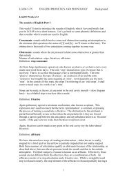
An example of a ray-traced image that typically takes seconds or
minutes to render.
These are attempts to simulate visual phenomena resulting from the optical characteristics of cameras and of the
human eye. These effects can lend an element of realism to a scene, even if the effect is merely a simulated artifact
of a camera. This is the basic method employed in games, interactive worlds and VRML. The rapid increase in
computer processing power has allowed a progressively higher degree of realism even for real-time rendering,
including techniques such as HDR rendering. Real-time rendering is often polygonal and aided by the computer's
GPU.
1

3D rendering 2
Non real-time
Animations for non-interactive media, such as feature
films and video, are rendered much more slowly.
Non-real time rendering enables the leveraging of
limited processing power in order to obtain higher
image quality. Rendering times for individual frames
may vary from a few seconds to several days for
complex scenes. Rendered frames are stored on a hard
disk then can be transferred to other media such as
motion picture film or optical disk. These frames are
then displayed sequentially at high frame rates,
typically 24, 25, or 30 frames per second, to achieve
the illusion of movement.
When the goal is photo-realism, techniques such as ray
tracing or radiosity are employed. This is the basic
Computer-generated image created by Gilles Tran.
method employed in digital media and artistic works. Techniques have been developed for the purpose of simulating
other naturally-occurring effects, such as the interaction of light with various forms of matter. Examples of such
techniques include particle systems (which can simulate rain, smoke, or fire), volumetric sampling (to simulate fog,
dust and other spatial atmospheric effects), caustics (to simulate light focusing by uneven light-refracting surfaces,
such as the light ripples seen on the bottom of a swimming pool), and subsurface scattering (to simulate light
reflecting inside the volumes of solid objects such as human skin).
The rendering process is computationally expensive, given the complex variety of physical processes being
simulated. Computer processing power has increased rapidly over the years, allowing for a progressively higher
degree of realistic rendering. Film studios that produce computer-generated animations typically make use of a
render farm to generate images in a timely manner. However, falling hardware costs mean that it is entirely possible
to create small amounts of 3D animation on a home computer system. The output of the renderer is often used as
only one small part of a completed motion-picture scene. Many layers of material may be rendered separately and
integrated into the final shot using compositing software.
Reflection and shading models
Models of reflection/scattering and shading are used to describe the appearance of a surface. Although these issues
may seem like problems all on their own, they are studied almost exclusively within the context of rendering.
Modern 3D computer graphics rely heavily on a simplified reflection model called Phong reflection model (not to be
confused with Phong shading). In refraction of light, an important concept is the refractive index. In most 3D
programming implementations, the term for this value is "index of refraction," usually abbreviated "IOR." Shading
can be broken down into two orthogonal issues, which are often studied independently:
• Reflection/Scattering - How light interacts with the surface at a given point
• Shading - How material properties vary across the surface

3D rendering 3
Reflection
Reflection or scattering is the relationship
between incoming and outgoing
illumination at a given point. Descriptions
of scattering are usually given in terms of a
bidirectional scattering distribution function
or BSDF. Popular reflection rendering
techniques in 3D computer graphics include:
• Flat shading: A technique that shades
each polygon of an object based on the
polygon's "normal" and the position and
intensity of a light source.
• Gouraud shading: Invented by H.
Gouraud in 1971, a fast and
resource-conscious vertex shading
technique used to simulate smoothly
shaded surfaces.
The Utah teapot
• Texture mapping: A technique for simulating a large amount of surface detail by mapping images (textures) onto
polygons.
• Phong shading: Invented by Bui Tuong Phong, used to simulate specular highlights and smooth shaded surfaces.
• Bump mapping: Invented by Jim Blinn, a normal-perturbation technique used to simulate wrinkled surfaces.
• Cel shading: A technique used to imitate the look of hand-drawn animation.
Shading
Shading addresses how different types of scattering are distributed across the surface (i.e., which scattering function
applies where). Descriptions of this kind are typically expressed with a program called a shader. (Note that there is
some confusion since the word "shader" is sometimes used for programs that describe local geometric variation.) A
simple example of shading is texture mapping, which uses an image to specify the diffuse color at each point on a
surface, giving it more apparent detail.
Transport
Transport describes how illumination in a scene gets from one place to another. Visibility is a major component of
light transport.
Projection

3D rendering 4
The shaded three-dimensional objects
must be flattened so that the display
device - namely a monitor - can
display it in only two dimensions, this
process is called 3D projection. This is
done using projection and, for most
applications, perspective projection.
The basic idea behind perspective
projection is that objects that are
further away are made smaller in
relation to those that are closer to the
eye. Programs produce perspective by
Perspective Projection
multiplying a dilation constant raised to the power of the negative of the distance from the observer. A dilation
constant of one means that there is no perspective. High dilation constants can cause a "fish-eye" effect in which
image distortion begins to occur. Orthographic projection is used mainly in CAD or CAM applications where
scientific modeling requires precise measurements and preservation of the third dimension.
External links
• Art is the basis of Industrial Design [1]
• A Critical History of Computer Graphics and Animation [2]
• The ARTS: Episode 5 [3] An in depth interview with Legalize on the subject of the History of Computer Graphics.
(Available in MP3 audio format)
• CGSociety [4] The Computer Graphics Society
• How Stuff Works - 3D Graphics [5]
• History of Computer Graphics series of articles [6]
• Open Inventor by VSG [7] 3D Graphics Toolkit for Applications Developers
References
[1] http:/ / www. eapprentice. net/ index. php?option=com_content& view=article& id=159:art-project& catid=64:model-making
[2] http:/ / accad. osu. edu/ ~waynec/ history/ lessons. html
[3] http:/ / www. acid. org/ radio/ index. html#ARTS-EP05
[4] http:/ / www. cgsociety. org/
[5] http:/ / computer. howstuffworks. com/ 3dgraphics. htm
[6] http:/ / hem. passagen. se/ des/ hocg/ hocg_1960. htm
[7] http:/ / www. vsg3d. com/ vsg_prod_openinventor. php

Alpha mapping
Concepts
Alpha mapping is a technique in 3D computer graphics where an image is mapped (assigned) to a 3D object, and
designates certain areas of the object to be transparent or translucent. The transparency can vary in strength, based on
the image texture, which can be greyscale, or the alpha channel of an RGBA image texture.
Ambient occlusion
Ambient occlusion is a shading method used in 3D computer graphics which helps add realism to local reflection
models by taking into account attenuation of light due to occlusion. Ambient occlusion attempts to approximate the
way light radiates in real life, especially off what are normally considered non-reflective surfaces.
Unlike local methods like Phong shading, ambient occlusion is a global method, meaning the illumination at each
point is a function of other geometry in the scene. However, it is a very crude approximation to full global
illumination. The soft appearance achieved by ambient occlusion alone is similar to the way an object appears on an
overcast day.
Method of implementation
Ambient occlusion is most often calculated by casting rays in every direction from the surface. Rays which reach the
background or “sky” increase the brightness of the surface, whereas a ray which hits any other object contributes no
illumination. As a result, points surrounded by a large amount of geometry are rendered dark, whereas points with
little geometry on the visible hemisphere appear light.
Ambient occlusion is related to accessibility shading, which determines appearance based on how easy it is for a
surface to be touched by various elements (e.g., dirt, light, etc.). It has been popularized in production animation due
to its relative simplicity and efficiency. In the industry, ambient occlusion is often referred to as "sky light".
The ambient occlusion shading model has the nice property of offering a better perception of the 3d shape of the
displayed objects. This was shown in a paper [1] where the authors report the results of perceptual experiments
showing that depth discrimination under diffuse uniform sky lighting is superior to that predicted by a direct lighting
model.
5

Ambient occlusion 6
ambient occlusion diffuse only combined ambient and diffuse
The occlusion at a point on a surface with normal can be computed by integrating the visibility function
over the hemisphere with respect to projected solid angle:
where is the visibility function at , defined to be zero if is occluded in the direction and one otherwise,
and is the infinitesimal solid angle step of the integration variable . A variety of techniques are used to
approximate this integral in practice: perhaps the most straightforward way is to use the Monte Carlo method by
casting rays from the point and testing for intersection with other scene geometry (i.e., ray casting). Another
approach (more suited to hardware acceleration) is to render the view from by rasterizing black geometry against
a white background and taking the (cosine-weighted) average of rasterized fragments. This approach is an example
of a "gathering" or "inside-out" approach, whereas other algorithms (such as depth-map ambient occlusion) employ
"scattering" or "outside-in" techniques.
In addition to the ambient occlusion value, a "bent normal" vector is often generated, which points in the average
direction of unoccluded samples. The bent normal can be used to look up incident radiance from an environment
map to approximate image-based lighting. However, there are some situations in which the direction of the bent
normal is a misrepresentation of the dominant direction of illumination, e.g.,

Ambient occlusion 7
In this example the bent normal N b has an unfortunate direction, since it is pointing at an occluded surface.
In this example, light may reach the point p only from the left or right sides, but the bent normal points to the
average of those two sources, which is, unfortunately, directly toward the obstruction.
Awards
In 2010, Hayden Landis, Ken McGaugh and Hilmar Koch were awarded a Scientific and Technical Academy Award
for their work on ambient occlusion rendering. [2]
References
[1] Langer, M.S.; H. H. Buelthoff (2000). "Depth discrimination from shading under diffuse lighting". Perception 29 (6): 649–660.
doi:10.1068/p3060. PMID 11040949.
[2] Oscar 2010: Scientific and Technical Awards (http:/ / www. altfg. com/ blog/ awards/ oscar-2010-scientific-and-technical-awards-489/ ), Alt
Film Guide, Jan 7, 2010
External links
• Depth Map based Ambient Occlusion (http:/ / www. andrew-whitehurst. net/ amb_occlude. html)
• NVIDIA's accurate, real-time Ambient Occlusion Volumes (http:/ / research. nvidia. com/ publication/
ambient-occlusion-volumes)
• Assorted notes about ambient occlusion (http:/ / www. cs. unc. edu/ ~coombe/ research/ ao/ )
• Ambient Occlusion Fields (http:/ / www. tml. hut. fi/ ~janne/ aofields/ ) — real-time ambient occlusion using
cube maps
• PantaRay ambient occlusion used in the movie Avatar (http:/ / research. nvidia. com/ publication/
pantaray-fast-ray-traced-occlusion-caching-massive-scenes)
• Fast Precomputed Ambient Occlusion for Proximity Shadows (http:/ / hal. inria. fr/ inria-00379385) real-time
ambient occlusion using volume textures
• Dynamic Ambient Occlusion and Indirect Lighting (http:/ / download. nvidia. com/ developer/ GPU_Gems_2/
GPU_Gems2_ch14. pdf) a real time self ambient occlusion method from Nvidia's GPU Gems 2 book
• GPU Gems 3 : Chapter 12. High-Quality Ambient Occlusion (http:/ / http. developer. nvidia. com/ GPUGems3/
gpugems3_ch12. html)

Ambient occlusion 8
• ShadeVis (http:/ / vcg. sourceforge. net/ index. php/ ShadeVis) an open source tool for computing ambient
occlusion
• xNormal (http:/ / www. xnormal. net) A free normal mapper/ambient occlusion baking application
• 3dsMax Ambient Occlusion Map Baking (http:/ / www. mrbluesummers. com/ 893/ video-tutorials/
baking-ambient-occlusion-in-3dsmax-monday-movie) Demo video about preparing ambient occlusion in 3dsMax
Anisotropic filtering
In 3D computer graphics, anisotropic
filtering (abbreviated AF) is a method
of enhancing the image quality of
textures on surfaces that are at oblique
viewing angles with respect to the
camera where the projection of the
texture (not the polygon or other
primitive on which it is rendered)
appears to be non-orthogonal (thus the
origin of the word: "an" for not, "iso"
for same, and "tropic" from tropism,
relating to direction; anisotropic
filtering does not filter the same in
every direction).
Like bilinear and trilinear filtering,
anisotropic filtering eliminates aliasing
effects, but improves on these other
techniques by reducing blur and
preserving detail at extreme viewing angles.
An illustration of texture filtering methods showing a trilinear mipmapped texture on the
left and the same texture enhanced with anisotropic texture filtering on the right.
Anisotropic compression is relatively intensive (primarily memory bandwidth and to some degree computationally,
though the standard space-time tradeoff rules apply) and only became a standard feature of consumer-level graphics
cards in the late 1990s. Anisotropic filtering is now common in modern graphics hardware (and video driver
software) and is enabled either by users through driver settings or by graphics applications and video games through
programming interfaces.

Anisotropic filtering 9
An improvement on isotropic MIP mapping
Hereafter, it is assumed the reader is familiar with
MIP mapping.
If we were to explore a more approximate anisotropic
algorithm, RIP mapping, as an extension from MIP
mapping, we can understand how anisotropic filtering
gains so much texture mapping quality. If we need to
texture a horizontal plane which is at an oblique angle
to the camera, traditional MIP map minification
would give us insufficient horizontal resolution due to
the reduction of image frequency in the vertical axis.
This is because in MIP mapping each MIP level is
isotropic, so a 256 × 256 texture is downsized to a 128
× 128 image, then a 64 × 64 image and so on, so
resolution halves on each axis simultaneously, so a
MIP map texture probe to an image will always
sample an image that is of equal frequency in each
axis. Thus, when sampling to avoid aliasing on a
high-frequency axis, the other texture axes will be
similarly downsampled and therefore potentially
blurred.
An example of ripmap image storage: the principal image on the top
left is accompanied by filtered, linearly transformed copies of reduced
With RIP map anisotropic filtering, in addition to downsampling to 128 × 128, images are also sampled to 256 × 128
and 32 × 128 etc. These *anisotropically* downsampled images can be probed when the texture-mapped image
frequency is different for each texture axis and therefore one axis need not blur due to the screen frequency of
another axis and aliasing is still avoided. Unlike more general anisotropic filtering, the RIP mapping described for
illustration has a limitation in that it only supports anisotropic probes that are axis-aligned in texture space, so
diagonal anisotropy still presents a problem even though real-use cases of anisotropic texture commonly have such
screenspace mappings.
In layman's terms, anisotropic filtering retains the "sharpness" of a texture normally lost by MIP map texture's
attempts to avoid aliasing. Anisotropic filtering can therefore be said to maintain crisp texture detail at all viewing
orientations while providing fast anti-aliased texture filtering.
Degree of anisotropy supported
Different degrees or ratios of anisotropic filtering can be applied during rendering and current hardware rendering
implementations set an upper bound on this ratio. This degree refers to the maximum ratio of anisotropy supported
by the filtering process. So, for example 4:1 (pronounced 4 to 1) anisotropic filtering will continue to sharpen more
oblique textures beyond the range sharpened by 2:1.
In practice what this means is that in highly oblique texturing situations a 4:1 filter will be twice as sharp as a 2:1
filter (it will display frequencies double that of the 2:1 filter). However, most of the scene will not require the 4:1
filter; only the more oblique and usually more distant pixels will require the sharper filtering. This means that as the
degree of anisotropic filtering continues to double there are diminishing returns in terms of visible quality with fewer
and fewer rendered pixels affected, and the results become less obvious to the viewer.
When one compares the rendered results of an 8:1 anisotropically filtered scene to a 16:1 filtered scene, only a
relatively few highly oblique pixels, mostly on more distant geometry, will display visibly sharper textures in the
scene with the higher degree of anisotropic filtering, and the frequency information on these few 16:1 filtered pixels
size.

Anisotropic filtering 10
will only be double that of the 8:1 filter. The performance penalty also diminishes because fewer pixels require the
data fetches of greater anisotropy.
In the end it is the additional hardware complexity vs. these diminishing returns, which causes an upper bound to be
set on the anisotropic quality in a hardware design. Applications and users are then free to adjust this trade-off
through driver and software settings up to this threshold.
Implementation
True anisotropic filtering probes the texture anisotropically on the fly on a per-pixel basis for any orientation of
anisotropy.
In graphics hardware, typically when the texture is sampled anisotropically, several probes (texel samples) of the
texture around the center point are taken, but on a sample pattern mapped according to the projected shape of the
texture at that pixel.
Each anisotropic filtering probe is often in itself a filtered MIP map sample, which adds more sampling to the
process. Sixteen trilinear anisotropic samples might require 128 samples from the stored texture, as trilinear MIP
map filtering needs to take four samples times two MIP levels and then anisotropic sampling (at 16-tap) needs to
take sixteen of these trilinear filtered probes.
However, this level of filtering complexity is not required all the time. There are commonly available methods to
reduce the amount of work the video rendering hardware must do.
Performance and optimization
The sample count required can make anisotropic filtering extremely bandwidth-intensive. Multiple textures are
common; each texture sample could be four bytes or more, so each anisotropic pixel could require 512 bytes from
texture memory, although texture compression is commonly used to reduce this.
As a video display device can easily contain over a million pixels, and as the desired frame rate can be as high as
30–60 frames per second (or more) the texture memory bandwidth can become very high very quickly. Ranges of
hundreds of gigabytes per second of pipeline bandwidth for texture rendering operations is not unusual where
anisotropic filtering operations are involved.
Fortunately, several factors mitigate in favor of better performance:
• The probes themselves share cached texture samples, both inter-pixel and intra-pixel.
• Even with 16-tap anisotropic filtering, not all 16 taps are always needed because only distant highly oblique pixel
fills tend to be highly anisotropic.
• Highly Anisotropic pixel fill tends to cover small regions of the screen (i.e. generally under 10%)
• Texture magnification filters (as a general rule) require no anisotropic filtering.
External links
• The Naked Truth About Anisotropic Filtering [1]
References
[1] http:/ / www. extremetech. com/ computing/ 51994-the-naked-truth-about-anisotropic-filtering

Back-face culling 11
Back-face culling
In computer graphics, back-face culling determines whether a polygon of a graphical object is visible. It is a step in
the graphical pipeline that tests whether the points in the polygon appear in clockwise or counter-clockwise order
when projected onto the screen. If the user has specified that front-facing polygons have a clockwise winding, if the
polygon projected on the screen has a counter-clockwise winding it has been rotated to face away from the camera
and will not be drawn.
The process makes rendering objects quicker and more efficient by reducing the number of polygons for the program
to draw. For example, in a city street scene, there is generally no need to draw the polygons on the sides of the
buildings facing away from the camera; they are completely occluded by the sides facing the camera.
A related technique is clipping, which determines whether polygons are within the camera's field of view at all.
Another similar technique is Z-culling, also known as occlusion culling, which attempts to skip the drawing of
polygons which are covered from the viewpoint by other visible polygons.
This technique only works with single-sided polygons, which are only visible from one side. Double-sided polygons
are rendered from both sides, and thus have no back-face to cull.
One method of implementing back-face culling is by discarding all polygons where the dot product of their surface
normal and the camera-to-polygon vector is greater than or equal to zero.
Further reading
• Geometry Culling in 3D Engines [1] , by Pietari Laurila
References
[1] http:/ / www. gamedev. net/ reference/ articles/ article1212. asp

Beam tracing 12
Beam tracing
Beam tracing is an algorithm to simulate wave propagation. It was developed in the context of computer graphics to
render 3D scenes, but it has been also used in other similar areas such as acoustics and electromagnetism
simulations.
Beam tracing is a derivative of the ray tracing algorithm that replaces rays, which have no thickness, with beams.
Beams are shaped like unbounded pyramids, with (possibly complex) polygonal cross sections. Beam tracing was
first proposed by Paul Heckbert and Pat Hanrahan [1] .
In beam tracing, a pyramidal beam is initially cast through the entire viewing frustum. This initial viewing beam is
intersected with each polygon in the environment, typically from nearest to farthest. Each polygon that intersects
with the beam must be visible, and is removed from the shape of the beam and added to a render queue. When a
beam intersects with a reflective or refractive polygon, a new beam is created in a similar fashion to ray-tracing.
A variant of beam tracing casts a pyramidal beam through each pixel of the image plane. This is then split up into
sub-beams based on its intersection with scene geometry. Reflection and transmission (refraction) rays are also
replaced by beams. This sort of implementation is rarely used, as the geometric processes involved are much more
complex and therefore expensive than simply casting more rays through the pixel.
Beam tracing solves certain problems related to sampling and aliasing, which can plague conventional ray tracing
approaches [2] . Since beam tracing effectively calculates the path of every possible ray within each beam [3] (which
can be viewed as a dense bundle of adjacent rays), it is not as prone to under-sampling (missing rays) or
over-sampling (wasted computational resources). The computational complexity associated with beams has made
them unpopular for many visualization applications. In recent years, Monte Carlo algorithms like distributed ray
tracing have become more popular for rendering calculations.
A 'backwards' variant of beam tracing casts beams from the light source into the environment. Similar to backwards
raytracing and photon mapping, backwards beam tracing may be used to efficiently model lighting effects such as
caustics [4] . Recently the backwards beam tracing technique has also been extended to handle glossy to diffuse
material interactions (glossy backward beam tracing) such as from polished metal surfaces [5] .
Beam tracing has been successfully applied to the fields of acoustic modelling [6] and electromagnetic propagation
modelling [7] . In both of these applications, beams are used as an efficient way to track deep reflections from a
source to a receiver (or vice-versa). Beams can provide a convenient and compact way to represent visibility. Once a
beam tree has been calculated, one can use it to readily account for moving transmitters or receivers.
Beam tracing is related in concept to cone tracing.
References
[1] P. S. Heckbert and P. Hanrahan, "Beam tracing polygonal objects", Computer Graphics 18(3), 119-127 (1984).
[2] A. Lehnert, "Systematic errors of the ray-tracing algorithm", Applied Acoustics 38, 207-221 (1993).
[3] Steven Fortune, "Topological Beam Tracing", Symposium on Computational Geometry 1999: 59-68
[4] M. Watt, "Light-water interaction using backwards beam tracing", in "Proceedings of the 17th annual conference on Computer graphics and
interactive techniques(SIGGRAPH'90)",377-385(1990).
[5] B. Duvenhage, K. Bouatouch, and D.G. Kourie, "Exploring the use of Glossy Light Volumes for Interactive Global Illumination", in
"Proceedings of the 7th International Conference on Computer Graphics, Virtual Reality, Visualisation and Interaction in Africa", 2010.
[6] T. Funkhouser, I. Carlbom, G. Elko, G. Pingali, M. Sondhi, and J. West, "A beam tracing approach to acoustic modelling for interactive
virtual environments", in Proceedings of the 25th annual conference on Computer graphics and interactive techniques (SIGGRAPH'98),
21-32 (1998).
[7] Steven Fortune, "A Beam-Tracing Algorithm for Prediction of Indoor Radio Propagation", in WACG 1996: 157-166

Bidirectional texture function 13
Bidirectional texture function
Bidirectional texture function (BTF) [1] is a 7-dimensional function depending on planar texture coordinates (x,y)
as well as on view and illumination spherical angles. In practice this function is obtained as a set of several
thousands color images of material sample taken during different camera and light positions.
To cope with a massive BTF data with high redundancy, many compression method were proposed [1] [2] .
Its main application is a photorealistic material rendering of objects in virtual reality systems.
References
[1] Jiří Filip; Michal Haindl (2009). "Bidirectional Texture Function Modeling: A State of the Art Survey" (http:/ / www. computer. org/ portal/
web/ csdl/ doi/ 10. 1109/ TPAMI. 2008. 246). IEEE Transactions on Pattern Analysis and Machine Intelligence, vol. 31, no. 11. pp.
1921–1940. .
[2] Vlastimil Havran; Jiří Filip, Karol Myszkowski (2009). "Bidirectional Texture Function Compression based on Multi-Level Vector
Quantization" (http:/ / www3. interscience. wiley. com/ journal/ 123233573/ abstract). Computer Graphics Forum, vol. 29, no. 1. pp.
175–190. .
Bilinear filtering
Bilinear filtering is a texture filtering method used to smooth textures
when displayed larger or smaller than they actually are.
Most of the time, when drawing a textured shape on the screen, the
texture is not displayed exactly as it is stored, without any distortion.
Because of this, most pixels will end up needing to use a point on the
texture that's 'between' texels, assuming the texels are points (as
opposed to, say, squares) in the middle (or on the upper left corner, or
anywhere else; it doesn't matter, as long as it's consistent) of their
A zoomed small portion of a bitmap, using
nearest-neighbor filtering (left), bilinear filtering
(center), and bicubic filtering (right).
respective 'cells'. Bilinear filtering uses these points to perform bilinear interpolation between the four texels nearest
to the point that the pixel represents (in the middle or upper left of the pixel, usually).
The formula
In these equations, u k and v k are the texture coordinates and y k is the color value at point k. Values without a
subscript refer to the pixel point; values with subscripts 0, 1, 2, and 3 refer to the texel points, starting at the top left,
reading right then down, that immediately surround the pixel point. So y 0 is the color of the texel at texture
coordinate (u 0 , v 0 ). These are linear interpolation equations. We'd start with the bilinear equation, but since this is a
special case with some elegant results, it is easier to start from linear interpolation.
Assuming that the texture is a square bitmap,

Bilinear filtering 14
Are all true. Further, define
With these we can simplify the interpolation equations:
And combine them:
Or, alternatively:
Which is rather convenient. However, if the image is merely scaled (and not rotated, sheared, put into perspective, or
any other manipulation), it can be considerably faster to use the separate equations and store y b (and sometimes y a , if
we are increasing the scale) for use in subsequent rows.
Sample code
This code assumes that the texture is square (an extremely common occurrence), that no mipmapping comes into
play, and that there is only one channel of data (not so common. Nearly all textures are in color so they have red,
green, and blue channels, and many have an alpha transparency channel, so we must make three or four calculations
of y, one for each channel).
{
double getBilinearFilteredPixelColor(Texture tex, double u, double v)
u *= tex.size;
v *= tex.size;
int x = floor(u);
int y = floor(v);
double u_ratio = u - x;
double v_ratio = v - y;
double u_opposite = 1 - u_ratio;
double v_opposite = 1 - v_ratio;
double result = (tex[x][y] * u_opposite + tex[x+1][y] *
u_ratio) * v_opposite +
u_ratio) * v_ratio;
}
return result;
(tex[x][y+1] * u_opposite + tex[x+1][y+1] *

Bilinear filtering 15
Limitations
Bilinear filtering is rather accurate until the scaling of the texture gets below half or above double the original size of
the texture - that is, if the texture was 256 pixels in each direction, scaling it to below 128 or above 512 pixels can
make the texture look bad, because of missing pixels or too much smoothness. Often, mipmapping is used to provide
a scaled-down version of the texture for better performance; however, the transition between two differently-sized
mipmaps on a texture in perspective using bilinear filtering can be very abrupt. Trilinear filtering, though somewhat
more complex, can make this transition smooth throughout.
For a quick demonstration of how a texel can be missing from a filtered texture, here's a list of numbers representing
the centers of boxes from an 8-texel-wide texture (in red and black), intermingled with the numbers from the centers
of boxes from a 3-texel-wide down-sampled texture (in blue). The red numbers represent texels that would not be
used in calculating the 3-texel texture at all.
0.0625, 0.1667, 0.1875, 0.3125, 0.4375, 0.5000, 0.5625, 0.6875, 0.8125, 0.8333, 0.9375
Special cases
Textures aren't infinite, in general, and sometimes one ends up with a pixel coordinate that lies outside the grid of
texel coordinates. There are a few ways to handle this:
• Wrap the texture, so that the last texel in a row also comes right before the first, and the last texel in a column also
comes right above the first. This works best when the texture is being tiled.
• Make the area outside the texture all one color. This may be of use for a texture designed to be laid over a solid
background or to be transparent.
• Repeat the edge texels out to infinity. This works best if the texture is not designed to be repeated.
Binary space partitioning
In computer science, binary space partitioning (BSP) is a method for recursively subdividing a space into convex
sets by hyperplanes. This subdivision gives rise to a representation of the scene by means of a tree data structure
known as a BSP tree.
Originally, this approach was proposed in 3D computer graphics to increase the rendering efficiency by
precomputing the BSP tree prior to low-level rendering operations. Some other applications include performing
geometrical operations with shapes (constructive solid geometry) in CAD, collision detection in robotics and 3D
computer games, and other computer applications that involve handling of complex spatial scenes.
Overview
In computer graphics it is desirable that the drawing of a scene be done both correctly and quickly. A simple way to
draw a scene is the painter's algorithm: draw it from back to front painting over the background with each closer
object. However, that approach is quite limited, since time is wasted drawing objects that will be overdrawn later,
and not all objects will be drawn correctly.
Z-buffering can ensure that scenes are drawn correctly and eliminate the ordering step of the painter's algorithm, but
it is expensive in terms of memory use. BSP trees will split up objects so that the painter's algorithm will draw them
correctly without need of a Z-buffer and eliminate the need to sort the objects; as a simple tree traversal will yield
them in the correct order. It also serves as a basis for other algorithms, such as visibility lists, which attempt to
reduce overdraw.
The downside is the requirement for a time consuming pre-processing of the scene, which makes it difficult and
inefficient to directly implement moving objects into a BSP tree. This is often overcome by using the BSP tree

Binary space partitioning 16
together with a Z-buffer, and using the Z-buffer to correctly merge movable objects such as doors and characters
onto the background scene.
BSP trees are often used by 3D computer games, particularly first-person shooters and those with indoor
environments. Probably the earliest game to use a BSP data structure was Doom (see Doom engine for an in-depth
look at Doom's BSP implementation). Other uses include ray tracing and collision detection.
Generation
Binary space partitioning is a generic process of recursively dividing a scene into two until the partitioning satisfies
one or more requirements. The specific method of division varies depending on its final purpose. For instance, in a
BSP tree used for collision detection, the original object would be partitioned until each part becomes simple enough
to be individually tested, and in rendering it is desirable that each part be convex so that the painter's algorithm can
be used.
The final number of objects will inevitably increase since lines or faces that cross the partitioning plane must be split
into two, and it is also desirable that the final tree remains reasonably balanced. Therefore the algorithm for correctly
and efficiently creating a good BSP tree is the most difficult part of an implementation. In 3D space, planes are used
to partition and split an object's faces; in 2D space lines split an object's segments.
The following picture illustrates the process of partitioning an irregular polygon into a series of convex ones. Notice
how each step produces polygons with fewer segments until arriving at G and F, which are convex and require no
further partitioning. In this particular case, the partitioning line was picked between existing vertices of the polygon
and intersected none of its segments. If the partitioning line intersects a segment, or face in a 3D model, the
offending segment(s) or face(s) have to be split into two at the line/plane because each resulting partition must be a
full, independent object.
1. A is the root of the tree and the entire polygon
2. A is split into B and C
3. B is split into D and E.
4. D is split into F and G, which are convex and hence become leaves on the tree.
Since the usefulness of a BSP tree depends upon how well it was generated, a good algorithm is essential. Most
algorithms will test many possibilities for each partition until they find a good compromise. They might also keep
backtracking information in memory, so that if a branch of the tree is found to be unsatisfactory, other alternative
partitions may be tried. Thus producing a tree usually requires long computations.
BSP trees are also used to represent natural images. Construction methods for BSP trees representing images were
first introduced as efficient representations in which only a few hundred nodes can represent an image that normally

Binary space partitioning 17
requires hundreds of thousands of pixels. Fast algorithms have also been developed to construct BSP trees of images
using computer vision and signal processing algorithms. These algorithms, in conjunction with advanced entropy
coding and signal approximation approaches, were used to develop image compression methods.
Rendering a scene with visibility information from the BSP tree
BSP trees are used to improve rendering performance in calculating visible triangles for the painter's algorithm for
instance. The tree can be traversed in linear time from an arbitrary viewpoint.
Since a painter's algorithm works by drawing polygons farthest from the eye first, the following code recurses to the
bottom of the tree and draws the polygons. As the recursion unwinds, polygons closer to the eye are drawn over far
polygons. Because the BSP tree already splits polygons into trivial pieces, the hardest part of the painter's algorithm
is already solved - code for back to front tree traversal. [1]
traverse_tree(bsp_tree* tree, point eye)
{
}
location = tree->find_location(eye);
if(tree->empty())
return;
if(location > 0) // if eye in front of location
{
}
traverse_tree(tree->back, eye);
display(tree->polygon_list);
traverse_tree(tree->front, eye);
else if(location < 0) // eye behind location
{
}
traverse_tree(tree->front, eye);
display(tree->polygon_list);
traverse_tree(tree->back, eye);
else // eye coincidental with partition hyperplane
{
}
traverse_tree(tree->front, eye);
traverse_tree(tree->back, eye);

Binary space partitioning 18
Other space partitioning structures
BSP trees divide a region of space into two subregions at each node. They are related to quadtrees and octrees, which
divide each region into four or eight subregions, respectively.
Relationship Table
Name p s
Binary Space Partition 1 2
Quadtree 2 4
Octree 3 8
where p is the number of dividing planes used, and s is the number of subregions formed.
BSP trees can be used in spaces with any number of dimensions. Quadtrees and octrees are useful for subdividing 2-
and 3-dimensional spaces, respectively. Another kind of tree that behaves somewhat like a quadtree or octree, but is
useful in any number of dimensions, is the kd-tree.
Timeline
• 1969 Schumacker et al. published a report that described how carefully positioned planes in a virtual environment
could be used to accelerate polygon ordering. The technique made use of depth coherence, which states that a
polygon on the far side of the plane cannot, in any way, obstruct a closer polygon. This was used in flight
simulators made by GE as well as Evans and Sutherland. However, creation of the polygonal data organization
was performed manually by scene designer.
• 1980 Fuchs et al. [FUCH80] extended Schumacker’s idea to the representation of 3D objects in a virtual
environment by using planes that lie coincident with polygons to recursively partition the 3D space. This provided
a fully automated and algorithmic generation of a hierarchical polygonal data structure known as a Binary Space
Partitioning Tree (BSP Tree). The process took place as an off-line preprocessing step that was performed once
per environment/object. At run-time, the view-dependent visibility ordering was generated by traversing the tree.
• 1981 Naylor's Ph.D thesis containing a full development of both BSP trees and a graph-theoretic approach using
strongly connected components for pre-computing visibility, as well as the connection between the two methods.
BSP trees as a dimension independent spatial search structure was emphasized, with applications to visible
surface determination. The thesis also included the first empirical data demonstrating that the size of the tree and
the number of new polygons was reasonable (using a model of the Space Shuttle).
• 1983 Fuchs et al. describe a micro-code implementation of the BSP tree algorithm on an Ikonas frame buffer
system. This was the first demonstration of real-time visible surface determination using BSP trees.
• 1987 Thibault and Naylor described how arbitrary polyhedra may be represented using a BSP tree as opposed to
the traditional b-rep (boundary representation). This provided a solid representation vs. a surface
based-representation. Set operations on polyhedra were described using a tool, enabling Constructive Solid
Geometry (CSG) in real-time. This was the fore runner of BSP level design using brushes, introduced in the
Quake editor and picked up in the Unreal Editor.
• 1990 Naylor, Amanatides, and Thibault provide an algorithm for merging two bsp trees to form a new bsp tree
from the two original trees. This provides many benefits including: combining moving objects represented by
BSP trees with a static environment (also represented by a BSP tree), very efficient CSG operations on polyhedra,
exact collisions detection in O(log n * log n), and proper ordering of transparent surfaces contained in two
interpenetrating objects (has been used for an x-ray vision effect).

Binary space partitioning 19
• 1990 Teller and Séquin proposed the offline generation of potentially visible sets to accelerate visible surface
determination in orthogonal 2D environments.
• 1991 Gordon and Chen [CHEN91] described an efficient method of performing front-to-back rendering from a
BSP tree, rather than the traditional back-to-front approach. They utilised a special data structure to record,
efficiently, parts of the screen that have been drawn, and those yet to be rendered. This algorithm, together with
the description of BSP Trees in the standard computer graphics textbook of the day (Foley, Van Dam, Feiner and
Hughes) was used by John Carmack in the making of Doom.
• 1992 Teller’s PhD thesis described the efficient generation of potentially visible sets as a pre-processing step to
acceleration real-time visible surface determination in arbitrary 3D polygonal environments. This was used in
Quake and contributed significantly to that game's performance.
• 1993 Naylor answers the question of what characterizes a good BSP tree. He used expected case models (rather
than worst case analysis) to mathematically measure the expected cost of searching a tree and used this measure
to build good BSP trees. Intuitively, the tree represents an object in a multi-resolution fashion (more exactly, as a
tree of approximations). Parallels with Huffman codes and probabilistic binary search trees are drawn.
• 1993 Hayder Radha's PhD thesis described (natural) image representation methods using BSP trees. This includes
the development of an optimal BSP-tree construction framework for any arbitrary input image. This framework is
based on a new image transform, known as the Least-Square-Error (LSE) Partitioning Line (LPE) transform. H.
Radha' thesis also developed an optimal rate-distortion (RD) image compression framework and image
manipulation approaches using BSP trees.
References
• [FUCH80] H. Fuchs, Z. M. Kedem and B. F. Naylor. “On Visible Surface Generation by A Priori Tree
Structures.” ACM Computer Graphics, pp 124–133. July 1980.
• [THIBAULT87] W. Thibault and B. Naylor, "Set Operations on Polyhedra Using Binary Space Partitioning
Trees", Computer Graphics (Siggraph '87), 21(4), 1987.
• [NAYLOR90] B. Naylor, J. Amanatides, and W. Thibualt, "Merging BSP Trees Yields Polyhedral Set
Operations", Computer Graphics (Siggraph '90), 24(3), 1990.
• [NAYLOR93] B. Naylor, "Constructing Good Partitioning Trees", Graphics Interface (annual Canadian CG
conference) May, 1993.
• [CHEN91] S. Chen and D. Gordon. “Front-to-Back Display of BSP Trees.” [2] IEEE Computer Graphics &
Algorithms, pp 79–85. September 1991.
• [RADHA91] H. Radha, R. Leoonardi, M. Vetterli, and B. Naylor “Binary Space Partitioning Tree Representation
of Images,” Journal of Visual Communications and Image Processing 1991, vol. 2(3).
• [RADHA93] H. Radha, "Efficient Image Representation using Binary Space Partitioning Trees.", Ph.D. Thesis,
Columbia University, 1993.
• [RADHA96] H. Radha, M. Vetterli, and R. Leoonardi, “Image Compression Using Binary Space Partitioning
Trees,” IEEE Transactions on Image Processing, vol. 5, No.12, December 1996, pp. 1610–1624.
• [WINTER99] AN INVESTIGATION INTO REAL-TIME 3D POLYGON RENDERING USING BSP TREES.
Andrew Steven Winter. April 1999. available online
• Mark de Berg, Marc van Kreveld, Mark Overmars, and Otfried Schwarzkopf (2000). Computational Geometry
(2nd revised edition ed.). Springer-Verlag. ISBN 3-540-65620-0. Section 12: Binary Space Partitions:
pp. 251–265. Describes a randomized Painter's Algorithm.
• Christer Ericson: Real-Time Collision Detection (The Morgan Kaufmann Series in Interactive 3-D Technology).
Verlag Morgan Kaufmann, S. 349-382, Jahr 2005, ISBN 1-55860-732-3

Binary space partitioning 20
[1] Binary Space Partition Trees in 3d worlds (http:/ / web. cs. wpi. edu/ ~matt/ courses/ cs563/ talks/ bsp/ document. html)
[2] http:/ / www. rothschild. haifa. ac. il/ ~gordon/ ftb-bsp. pdf
External links
• BSP trees presentation (http:/ / www. cs. wpi. edu/ ~matt/ courses/ cs563/ talks/ bsp/ bsp. html)
• Another BSP trees presentation (http:/ / www. cc. gatech. edu/ classes/ AY2004/ cs4451a_fall/ bsp. pdf)
• A Java applet which demonstrates the process of tree generation (http:/ / symbolcraft. com/ graphics/ bsp/ )
• A Master Thesis about BSP generating (http:/ / www. gamedev. net/ reference/ programming/ features/ bsptree/
bsp. pdf)
• BSP Trees: Theory and Implementation (http:/ / www. devmaster. net/ articles/ bsp-trees/ )
• BSP in 3D space (http:/ / www. euclideanspace. com/ threed/ solidmodel/ spatialdecomposition/ bsp/ index. htm)
• A simple, illustrated introduction to using BSPs to create random room layouts (in this case for a
dungeon-crawling game) (http:/ / doryen. eptalys. net/ articles/ bsp-dungeon-generation/ )
Bounding interval hierarchy
A bounding interval hierarchy (BIH) is a partitioning data structure similar to that of bounding volume hierarchies
or kd-trees. Bounding interval hierarchies can be used in high performance (or real-time) ray tracing and may be
especially useful for dynamic scenes.
The BIH itself is, however, not new. It has been presented earlier under the name of SKD-Trees [1] , presented by
Ooi et al., and BoxTrees [2] , independently invented by Zachmann.
Overview
Bounding interval hierarchies (BIH) exhibit many of the properties of both bounding volume hierarchies (BVH) and
kd-trees. Whereas the construction and storage of BIH is comparable to that of BVH, the traversal of BIH resemble
that of kd-trees. Furthermore, BIH are also binary trees just like kd-trees (and in fact their superset, BSP trees).
Finally, BIH are axis-aligned as are its ancestors. Although a more general non-axis-aligned implementation of the
BIH should be possible (similar to the BSP-tree, which uses unaligned planes), it would almost certainly be less
desirable due to decreased numerical stability and an increase in the complexity of ray traversal.
The key feature of the BIH is the storage of 2 planes per node (as opposed to 1 for the kd tree and 6 for an axis
aligned bounding box hierarchy), which allows for overlapping children (just like a BVH), but at the same time
featuring an order on the children along one dimension/axis (as it is the case for kd trees).
It is also possible to just use the BIH data structure for the construction phase but traverse the tree in a way a
traditional axis aligned bounding box hierarchy does. This enables some simple speed up optimizations for large ray
bundles [3] while keeping memory/cache usage low.
Some general attributes of bounding interval hierarchies (and techniques related to BIH) as described by [4] are:
• Very fast construction times
• Low memory footprint
• Simple and fast traversal
• Very simple construction and traversal algorithms
• High numerical precision during construction and traversal
• Flatter tree structure (decreased tree depth) compared to kd-trees

Bounding interval hierarchy 21
Operations
Construction
To construct any space partitioning structure some form of heuristic is commonly used. For this the surface area
heuristic, commonly used with many partitioning schemes, is a possible candidate. Another, more simplistic
heuristic is the "global" heuristic described by [4] which only requires an axis-aligned bounding box, rather than the
full set of primitives, making it much more suitable for a fast construction.
The general construction scheme for a BIH:
• calculate the scene bounding box
• use a heuristic to choose one axis and a split plane candidate perpendicular to this axis
• sort the objects to the left or right child (exclusively) depending on the bounding box of the object (note that
objects intersecting the split plane may either be sorted by its overlap with the child volumes or any other
heuristic)
• calculate the maximum bounding value of all objects on the left and the minimum bounding value of those on the
right for that axis (can be combined with previous step for some heuristics)
• store these 2 values along with 2 bits encoding the split axis in a new node
• continue with step 2 for the children
Potential heuristics for the split plane candidate search:
• Classical: pick the longest axis and the middle of the node bounding box on that axis
• Classical: pick the longest axis and a split plane through the median of the objects (results in a leftist tree which is
often unfortunate for ray tracing though)
• Global heuristic: pick the split plane based on a global criterion, in the form of a regular grid (avoids unnecessary
splits and keeps node volumes as cubic as possible)
• Surface area heuristic: calculate the surface area and amount of objects for both children, over the set of all
possible split plane candidates, then choose the one with the lowest costs (claimed to be optimal, though the cost
function poses unusual demands to proof the formula, which can not be fulfilled in real life. also an exceptionally
slow heuristic to evaluate)
Ray traversal
The traversal phase closely resembles a kd-tree traversal: One has to distinguish 4 simple cases, where the ray
• just intersects the left child
• just intersects the right child
• intersects both children
• intersects none of both (the only case not possible in a kd traversal)
For the third case, depending on the ray direction (negative or positive) of the component (x, y or z) equalling the
split axis of the current node, the traversal continues first with the left (positive direction) or the right (negative
direction) child and the other one is pushed onto a stack.
Traversal continues until a leaf node is found. After intersecting the objects in the leaf, the next element is popped
from the stack. If the stack is empty, the nearest intersection of all pierced leafs is returned.
It is also possible to add a 5th traversal case, but which also requires a slightly complicated construction phase. By
swapping the meanings of the left and right plane of a node, it is possible to cut off empty space on both sides of a
node. This requires an additional bit that must be stored in the node to detect this special case during traversal.
Handling this case during the traversal phase is simple, as the ray
• just intersects the only child of the current node or
• intersects nothing

Bounding interval hierarchy 22
Properties
Numerical stability
All operations during the hierarchy construction/sorting of the triangles are min/max-operations and comparisons.
Thus no triangle clipping has to be done as it is the case with kd-trees and which can become a problem for triangles
that just slightly intersect a node. Even if the kd implementation is carefully written, numerical errors can result in a
non-detected intersection and thus rendering errors (holes in the geometry) due to the missed ray-object intersection.
Extensions
Instead of using two planes per node to separate geometry, it is also possible to use any number of planes to create a
n-ary BIH or use multiple planes in a standard binary BIH (one and four planes per node were already proposed in [4]
and then properly evaluated in [5] ) to achieve better object separation.
References
Papers
[1] Nam, Beomseok; Sussman, Alan. A comparative study of spatial indexing techniques for multidimensional scientific datasets (http:/ /
ieeexplore. ieee. org/ Xplore/ login. jsp?url=/ iel5/ 9176/ 29111/ 01311209. pdf)
[2] Zachmann, Gabriel. Minimal Hierarchical Collision Detection (http:/ / zach. in. tu-clausthal. de/ papers/ vrst02. html)
[3] Wald, Ingo; Boulos, Solomon; Shirley, Peter (2007). Ray Tracing Deformable Scenes using Dynamic Bounding Volume Hierarchies (http:/ /
www. sci. utah. edu/ ~wald/ Publications/ 2007/ / / BVH/ download/ / togbvh. pdf)
[4] Wächter, Carsten; Keller, Alexander (2006). Instant Ray Tracing: The Bounding Interval Hierarchy (http:/ / ainc. de/ Research/ BIH. pdf)
[5] Wächter, Carsten (2008). Quasi-Monte Carlo Light Transport Simulation by Efficient Ray Tracing (http:/ / vts. uni-ulm. de/ query/ longview.
meta. asp?document_id=6265)
Forums
• http:/ / ompf. org/ forum (http:/ / ompf. org/ forum)
External links
• BIH implementations: Javascript (http:/ / github. com/ imbcmdth/ jsBIH).

Bounding volume 23
Bounding volume
For building code compliance, see Bounding.
In computer graphics and computational geometry, a bounding
volume for a set of objects is a closed volume that completely contains
the union of the objects in the set. Bounding volumes are used to
improve the efficiency of geometrical operations by using simple
volumes to contain more complex objects. Normally, simpler volumes
have simpler ways to test for overlap.
A bounding volume for a set of objects is also a bounding volume for
the single object consisting of their union, and the other way around.
Therefore it is possible to confine the description to the case of a single
object, which is assumed to be non-empty and bounded (finite).
Uses of bounding volumes
Bounding volumes are most often used to accelerate certain kinds of tests.
A three dimensional model with its bounding box
drawn in dashed lines.
In ray tracing, bounding volumes are used in ray-intersection tests, and in many rendering algorithms, they are used
for viewing frustum tests. If the ray or viewing frustum does not intersect the bounding volume, it cannot intersect
the object contained in the volume. These intersection tests produce a list of objects that must be displayed. Here,
displayed means rendered or rasterized.
In collision detection, when two bounding volumes do not intersect, then the contained objects cannot collide, either.
Testing against a bounding volume is typically much faster than testing against the object itself, because of the
bounding volume's simpler geometry. This is because an 'object' is typically composed of polygons or data structures
that are reduced to polygonal approximations. In either case, it is computationally wasteful to test each polygon
against the view volume if the object is not visible. (Onscreen objects must be 'clipped' to the screen, regardless of
whether their surfaces are actually visible.)
To obtain bounding volumes of complex objects, a common way is to break the objects/scene down using a scene
graph or more specifically bounding volume hierarchies like e.g. OBB trees. The basic idea behind this is to organize
a scene in a tree-like structure where the root comprises the whole scene and each leaf contains a smaller subpart.
Common types of bounding volume
The choice of the type of bounding volume for a given application is determined by a variety of factors: the
computational cost of computing a bounding volume for an object, the cost of updating it in applications in which
the objects can move or change shape or size, the cost of determining intersections, and the desired precision of the
intersection test. The precision of the intersection test is related to the amount of space within the bounding volume
not associated with the bounded object, called void space. Sophisticated bounding volumes generally allow for less
void space but are more computationally expensive. It is common to use several types in conjunction, such as a
cheap one for a quick but rough test in conjunction with a more precise but also more expensive type.
The types treated here all give convex bounding volumes. If the object being bounded is known to be convex, this is
not a restriction. If non-convex bounding volumes are required, an approach is to represent them as a union of a
number of convex bounding volumes. Unfortunately, intersection tests become quickly more expensive as the

Bounding volume 24
bounding boxes become more sophisticated.
A bounding sphere is a sphere containing the object. In 2-D graphics, this is a circle. Bounding spheres are
represented by centre and radius. They are very quick to test for collision with each other: two spheres intersect
when the distance between their centres does not exceed the sum of their radii. This makes bounding spheres
appropriate for objects that can move in any number of dimensions.
A bounding ellipsoid is an ellipsoid containing the object. Ellipsoids usually provide tighter fitting than a sphere.
Intersections with ellipsoids are done by scaling the other object along the principal axes of the ellipsoid by an
amount equal to the multiplicative inverse of the radii of the ellipsoid, thus reducing the problem to intersecting the
scaled object with a unit sphere. Care should be taken to avoid problems if the applied scaling introduces skew.
Skew can make the usage of ellipsoids impractical in certain cases, for example collision between two arbitrary
ellipsoids.
A bounding cylinder is a cylinder containing the object. In most applications the axis of the cylinder is aligned with
the vertical direction of the scene. Cylinders are appropriate for 3-D objects that can only rotate about a vertical axis
but not about other axes, and are otherwise constrained to move by translation only. Two vertical-axis-aligned
cylinders intersect when, simultaneously, their projections on the vertical axis intersect – which are two line
segments – as well their projections on the horizontal plane – two circular disks. Both are easy to test. In video
games, bounding cylinders are often used as bounding volumes for people standing upright.
A bounding capsule is a swept sphere (i.e. the volume that a sphere takes as it moves along a straight line segment)
containing the object. Capsules can be represented by the radius of the swept sphere and the segment that the sphere
is swept across). It has traits similar to a cylinder, but is easier to use, because the intersection test is simpler. A
capsule and another object intersect if the distance between the capsule's defining segment and some feature of the
other object is smaller than the capsule's radius. For example, two capsules intersect if the distance between the
capsules' segments is smaller than the sum of their radii. This holds for arbitrarily rotated capsules, which is why
they're more appealing than cylinders in practice.
A bounding box is a cuboid, or in 2-D a rectangle, containing the object. In dynamical simulation, bounding boxes
are preferred to other shapes of bounding volume such as bounding spheres or cylinders for objects that are roughly
cuboid in shape when the intersection test needs to be fairly accurate. The benefit is obvious, for example, for objects
that rest upon other, such as a car resting on the ground: a bounding sphere would show the car as possibly
intersecting with the ground, which then would need to be rejected by a more expensive test of the actual model of
the car; a bounding box immediately shows the car as not intersecting with the ground, saving the more expensive
test.
In many applications the bounding box is aligned with the axes of the co-ordinate system, and it is then known as an
axis-aligned bounding box (AABB). To distinguish the general case from an AABB, an arbitrary bounding box is
sometimes called an oriented bounding box (OBB). AABBs are much simpler to test for intersection than OBBs,
but have the disadvantage that when the model is rotated they cannot be simply rotated with it, but need to be
recomputed.
A bounding slab is related to the AABB and used to speed up ray tracing [1]
A minimum bounding rectangle or MBR – the least AABB in 2-D – is frequently used in the description of
geographic (or "geospatial") data items, serving as a simplified proxy for a dataset's spatial extent (see geospatial
metadata) for the purpose of data search (including spatial queries as applicable) and display. It is also a basic
component of the R-tree method of spatial indexing.
A discrete oriented polytope (DOP) generalizes the AABB. A DOP is a convex polytope containing the object (in
2-D a polygon; in 3-D a polyhedron), constructed by taking a number of suitably oriented planes at infinity and
moving them until they collide with the object. The DOP is then the convex polytope resulting from intersection of
the half-spaces bounded by the planes. Popular choices for constructing DOPs in 3-D graphics include the

Bounding volume 25
axis-aligned bounding box, made from 6 axis-aligned planes, and the beveled bounding box, made from 10 (if
beveled only on vertical edges, say) 18 (if beveled on all edges), or 26 planes (if beveled on all edges and corners). A
DOP constructed from k planes is called a k-DOP; the actual number of faces can be less than k, since some can
become degenerate, shrunk to an edge or a vertex.
A convex hull is the smallest convex volume containing the object. If the object is the union of a finite set of points,
its convex hull is a polytope.
Basic intersection checks
For some types of bounding volume (OBB and convex polyhedra), an effective check is that of the separating axis
theorem. The idea here is that, if there exists an axis by which the objects do not overlap, then the objects do not
intersect. Usually the axes checked are those of the basic axes for the volumes (the unit axes in the case of an AABB,
or the 3 base axes from each OBB in the case of OBBs). Often, this is followed by also checking the cross-products
of the previous axes (one axis from each object).
In the case of an AABB, this tests becomes a simple set of overlap tests in terms of the unit axes. For an AABB
defined by M,N against one defined by O,P they do not intersect if (M x >P x ) or (O x >N x ) or (M y >P y ) or (O y >N y ) or
(M z >P z ) or (O z >N z ).
An AABB can also be projected along an axis, for example, if it has edges of length L and is centered at C, and is
being projected along the axis N:
, and or , and
where m and n are the minimum and maximum extents.
An OBB is similar in this respect, but is slightly more complicated. For an OBB with L and C as above, and with I, J,
and K as the OBB's base axes, then:
For the ranges m,n and o,p it can be said that they do not intersect if m>p or o>n. Thus, by projecting the ranges of 2
OBBs along the I, J, and K axes of each OBB, and checking for non-intersection, it is possible to detect
non-intersection. By additionally checking along the cross products of these axes (I 0 ×I 1 , I 0 ×J 1 , ...) one can be more
certain that intersection is impossible.
This concept of determining non-intersection via use of axis projection also extends to convex polyhedra, however
with the normals of each polyhedral face being used instead of the base axes, and with the extents being based on the
minimum and maximum dot products of each vertex against the axes. Note that this description assumes the checks
are being done in world space.
References
[1] POV-Ray Documentation (http:/ / www. povray. org/ documentation/ view/ 3. 6. 1/ 323/ )
External links
• Illustration of several DOPs for the same model, from epicgames.com (http:/ / udn. epicgames. com/ Two/ rsrc/
Two/ CollisionTutorial/ kdop_sizes. jpg)

Bump mapping 26
Bump mapping
Bump mapping is a technique in
computer graphics for simulating
bumps and wrinkles on the surface of
an object. This is achieved by
perturbing the surface normals of the
object and using the perturbed normal
during lighting calculations. The result
is an apparently bumpy surface rather
than a smooth surface although the
surface of the underlying object is not
actually changed. Bump mapping was
introduced by Blinn in 1978. [1]
Normal mapping is the most common variation of bump mapping used [2] .
Bump mapping basics
Bump mapping is a technique in
computer graphics to make a rendered
surface look more realistic by
simulating small displacements of the
surface. However, unlike traditional
displacement mapping, the surface
geometry is not modified. Instead only
the surface normal is modified as if the
surface had been displaced. The
modified surface normal is then used
for lighting calculations as usual,
typically using the Phong reflection
model or similar, giving the
appearance of detail instead of a
smooth surface.
Bump mapping is much faster and
consumes less resources for the same
level of detail compared to
displacement mapping because the geometry remains unchanged.
A sphere without bump mapping (left). A bump map to be applied to the sphere (middle).
The sphere with the bump map applied (right) appears to have a mottled surface
resembling an orange. Bump maps achieve this effect by changing how an illuminated
surface reacts to light without actually modifying the size or shape of the surface
Bump mapping is limited in that it does not actually modify the shape of the underlying
object. On the left, a mathematical function defining a bump map simulates a crumbling
surface on a sphere, but the object's outline and shadow remain those of a perfect sphere.
On the right, the same function is used to modify the surface of a sphere by generating an
isosurface. This actually models a sphere with a bumpy surface with the result that both
its outline and its shadow are rendered realistically.
There are primarily two methods to perform bump mapping. The first uses a height map for simulating the surface
displacement yielding the modified normal. This is the method invented by Blinn [1] and is usually what is referred to
as bump mapping unless specified. The steps of this method is summarized as follows.
Before lighting a calculation is performed for each visible point (or pixel) on the object's surface:
1. Look up the height in the heightmap that corresponds to the position on the surface.
2. Calculate the surface normal of the heightmap, typically using the finite difference method.
3. Combine the surface normal from step two with the true ("geometric") surface normal so that the combined
normal points in a new direction.

Bump mapping 27
4. Calculate the interaction of the new "bumpy" surface with lights in the scene using, for example, the Phong
reflection model.
The result is a surface that appears to have real depth. The algorithm also ensures that the surface appearance
changes as lights in the scene are moved around.
The other method is to specify a normal map which contains the modified normal for each point on the surface
directly. Since the normal is specified directly instead of derived from a height map this method usually leads to
more predictable results. This makes it easier for artists to work with, making it the most common method of bump
mapping today [2] .
There are also extensions which modifies other surface features in addition to increase the sense of depth. Parallax
mapping is one such extension.
The primary limitation with bump mapping is that it perturbs only the surface normals without changing the
underlying surface itself. [3] Silhouettes and shadows therefore remain unaffected, which is especially noticeable for
larger simulated displacements. This limitation can be overcome by techniques including the displacement mapping
where bumps are actually applied to the surface or using an isosurface.
Realtime bump mapping techniques
Realtime 3D graphics programmers often use variations of the technique in order to simulate bump mapping at a
lower computational cost.
One typical way was to use a fixed geometry, which allows one to use the heightmap surface normal almost directly.
Combined with a precomputed lookup table for the lighting calculations the method could be implemented with a
very simple and fast loop, allowing for a full-screen effect. This method was a common visual effect when bump
mapping was first introduced.
References
[1] Blinn, James F. "Simulation of Wrinkled Surfaces" (http:/ / portal. acm. org/ citation. cfm?id=507101), Computer Graphics, Vol. 12 (3),
pp. 286-292 SIGGRAPH-ACM (August 1978)
[2] Mikkelsen, Morten. Simulation of Wrinkled Surfaces Revisited (http:/ / image. diku. dk/ projects/ media/ morten. mikkelsen. 08. pdf), 2008
(PDF)
[3] Real-Time Bump Map Synthesis (http:/ / web4. cs. ucl. ac. uk/ staff/ j. kautz/ publications/ rtbumpmapHWWS01. pdf), Jan Kautz 1 , Wolfgang
Heidrichy 2 and Hans-Peter Seidel 1 , ( 1 Max-Planck-Institut für Informatik, 2 University of British Columbia)
External links
• Bump shading for volume textures (http:/ / ieeexplore. ieee. org/ xpl/ freeabs_all. jsp?arnumber=291525), Max,
N.L., Becker, B.G., Computer Graphics and Applications, IEEE, Jul 1994, Volume 14, Issue 4, pages 18 - 20,
ISSN 0272-1716
• Bump Mapping tutorial using CG and C++ (http:/ / www. blacksmith-studios. dk/ projects/ downloads/
bumpmapping_using_cg. php)
• Simple creating vectors per pixel of a grayscale for a bump map to work and more (http:/ / freespace. virgin. net/
hugo. elias/ graphics/ x_polybm. htm)
• Bump Mapping example (http:/ / www. neilwallis. com/ java/ bump2. htm) (Java applet)

CatmullClark subdivision surface 28
Catmull–Clark subdivision surface
The Catmull–Clark algorithm is used in computer graphics to create
smooth surfaces by subdivision surface modeling. It was devised by
Edwin Catmull and Jim Clark in 1978 as a generalization of bi-cubic
uniform B-spline surfaces to arbitrary topology. [1] In 2005, Edwin
Catmull received an Academy Award for Technical Achievement
together with Tony DeRose and Jos Stam for their invention and
application of subdivision surfaces.
Recursive evaluation
Catmull–Clark surfaces are defined recursively, using the following
refinement scheme: [1]
Start with a mesh of an arbitrary polyhedron. All the vertices in this
mesh shall be called original points.
• For each face, add a face point
• Set each face point to be the centroid of all original points for the
respective face.
• For each edge, add an edge point.
First three steps of Catmull–Clark subdivision of
a cube with subdivision surface below
• Set each edge point to be the average of the two neighbouring face points and its two original endpoints.
• For each face point, add an edge for every edge of the face, connecting the face point to each edge point for the
face.
• For each original point P, take the average F of all n face points for faces touching P, and take the average R of all
n edge midpoints for edges touching P, where each edge midpoint is the average of its two endpoint vertices.
Move each original point to the point
(This is the barycenter of P, R and F with respective weights (n-3), 2 and 1. This arbitrary-looking formula was
chosen by Catmull and Clark based on the aesthetic appearance of the resulting surfaces rather than on a
mathematical derivation.)
The new mesh will consist only of quadrilaterals, which won't in general be planar. The new mesh will generally
look smoother than the old mesh.
Repeated subdivision results in smoother meshes. It can be shown that the limit surface obtained by this refinement
process is at least at extraordinary vertices and everywhere else (when n indicates how many derivatives are
continuous, we speak of continuity). After one iteration, the number of extraordinary points on the surface
remains constant.

CatmullClark subdivision surface 29
Exact evaluation
The limit surface of Catmull–Clark subdivision surfaces can also be evaluated directly, without any recursive
refinement. This can be accomplished by means of the technique of Jos Stam [2] . This method reformulates the
recursive refinement process into a matrix exponential problem, which can be solved directly by means of matrix
diagonalization.
Software using Catmull–Clark subdivision surfaces
• 3ds max
• 3D-Coat
• AC3D
• Anim8or
• Blender
• Carrara
• CATIA (Imagine and Shape)
• Cheetah3D
• Cinema4D
• DAZ Studio, 2.0
• DeleD Pro
• Gelato
• Hexagon
• Houdini
• JPatch
• K-3D
• LightWave 3D, version 9
• Maya
• modo
• Mudbox
• Realsoft3D
• Remo 3D
• Shade
• Silo
• SketchUp -Requires a Plugin.
• Softimage XSI
• Strata 3D CX
• Vue 9
• Wings 3D
• Zbrush
• TopMod
• TopoGun

CatmullClark subdivision surface 30
References
[1] E. Catmull and J. Clark: Recursively generated B-spline surfaces on arbitrary topological meshes, Computer-Aided Design 10(6):350-355
(November 1978), ( doi (http:/ / dx. doi. org/ 10. 1016/ 0010-4485(78)90110-0), pdf (http:/ / www. idi. ntnu. no/ ~fredrior/ files/
Catmull-Clark 1978 Recursively generated surfaces. pdf))
[2] Jos Stam, Exact Evaluation of Catmull–Clark Subdivision Surfaces at Arbitrary Parameter Values, Proceedings of SIGGRAPH'98. In
Computer Graphics Proceedings, ACM SIGGRAPH, 1998, 395–404 ( pdf (http:/ / www. dgp. toronto. edu/ people/ stam/ reality/ Research/
pdf/ sig98. pdf), downloadable eigenstructures (http:/ / www. dgp. toronto. edu/ ~stam/ reality/ Research/ SubdivEval/ index. html))
Conversion between quaternions and Euler
angles
Spatial rotations in three dimensions can be parametrized using both Euler angles and unit quaternions. This article
explains how to convert between the two representations. Actually this simple use of "quaternions" was first
presented by Euler some seventy years earlier than Hamilton to solve the problem of magic squares. For this reason
the dynamics community commonly refers to quaternions in this application as "Euler parameters".
Definition
A unit quaternion can be described as:
We can associate a quaternion with a rotation around an axis by the following expression
where α is a simple rotation angle (the value in radians of the angle of rotation) and cos(β x ), cos(β y ) and cos(β z ) are
the "direction cosines" locating the axis of rotation (Euler's Theorem).

Conversion between quaternions and Euler angles 31
Rotation matrices
Euler angles – The xyz (fixed) system is shown in blue, the XYZ (rotated) system
is shown in red. The line of nodes, labelled N, is shown in green.
The orthogonal matrix (post-multiplying a column vector) corresponding to a clockwise/left-handed rotation by the
unit quaternion is given by the inhomogeneous expression
or equivalently, by the homogeneous expression
If is not a unit quaternion then the homogeneous form is still a scalar multiple of a rotation
matrix, while the inhomogeneous form is in general no longer an orthogonal matrix. This is why in numerical work
the homogeneous form is to be preferred if distortion is to be avoided.
The orthogonal matrix (post-multiplying a column vector) corresponding to a clockwise/left-handed rotation with
Euler angles φ, θ, ψ, with x-y-z convention, is given by:

Conversion between quaternions and Euler angles 32
Conversion
By combining the quaternion representations of the Euler rotations we get
For Euler angles we get:
arctan and arcsin have a result between −π/2 and π/2. With three rotation between −π/2 and π/2 you can't have all
possible orientations. You need to replace the arctan by atan2 to generate all the orientation.
Relationship with Tait–Bryan angles
Similarly for Euler angles, we use the Tait–Bryan angles (in terms
of flight dynamics):
• Roll – : rotation about the X-axis
• Pitch – : rotation about the Y-axis
• Yaw – : rotation about the Z-axis
where the X-axis points forward, Y-axis to the right and Z-axis
downward and in the example to follow the rotation occurs in the
order yaw, pitch, roll (about body-fixed axes).
Singularities
One must be aware of singularities in the Euler angle
parametrization when the pitch approaches ±90° (north/south
pole). These cases must be handled specially. The common name
for this situation is gimbal lock.
Code to handle the singularities is derived on this site:
www.euclideanspace.com [1]
Tait–Bryan angles for an aircraft

Conversion between quaternions and Euler angles 33
External links
• Q60. How do I convert Euler rotation angles to a quaternion? [2] and related questions at The Matrix and
Quaternions FAQ
References
[1] http:/ / www. euclideanspace. com/ maths/ geometry/ rotations/ conversions/ quaternionToEuler/
[2] http:/ / www. j3d. org/ matrix_faq/ matrfaq_latest. html#Q60
Cube mapping
In computer graphics, cube mapping is a method of
environment mapping that uses a six-sided cube as the
map shape. The environment is projected onto the six
faces of a cube and stored as six square textures, or
unfolded into six regions of a single texture. The cube
map is generated by first rendering the scene six times
from a viewpoint, with the views defined by an
orthogonal 90 degree view frustum representing each
cube face. [1]
In the majority of cases, cube mapping is preferred
over the older method of sphere mapping because it
eliminates many of the problems that are inherent in
sphere mapping such as image distortion, viewpoint
dependency, and computational efficiency. Also, cube
mapping provides a much larger capacity to support
real-time rendering of reflections relative to sphere
mapping because the combination of inefficiency and
viewpoint dependency severely limit the ability of
sphere mapping to be applied when there is a
consistently changing viewpoint.
History
The lower left image shows a scene with a viewpoint marked with a
black dot. The upper image shows the net of the cube mapping as seen
from that viewpoint, and the lower right image shows the cube
superimposed on the original scene.
Cube mapping was first proposed in 1986 by Ned Greene in his paper “Environment Mapping and Other
Applications of World Projections” [2] , ten years after environment mapping was first put forward by Jim Blinn and
Martin Newell. However, hardware limitations on the ability to access six texture images simultaneously made it
infeasible to implement cube mapping without further technological developments. This problem was remedied in
1999 with the release of the Nvidia GeForce 256. Nvidia touted cube mapping in hardware as “a breakthrough image
quality feature of GeForce 256 that ... will allow developers to create accurate, real-time reflections. Accelerated in
hardware, cube environment mapping will free up the creativity of developers to use reflections and specular lighting
effects to create interesting, immersive environments.” [3] Today, cube mapping is still used in a variety of graphical
applications as a favored method of environment mapping.

Cube mapping 34
Advantages
Cube mapping is preferred over other methods of environment mapping because of its relative simplicity. Also, cube
mapping produces results that are similar to those obtained by ray tracing, but is much more computationally
efficient – the moderate reduction in quality is compensated for by large gains in efficiency.
Predating cube mapping, sphere mapping has many inherent flaws that made it impractical for most applications.
Sphere mapping is view dependent meaning that a different texture is necessary for each viewpoint. Therefore, in
applications where the viewpoint is mobile, it would be necessary to dynamically generate a new sphere mapping for
each new viewpoint (or, to pre-generate a mapping for every viewpoint). Also, a texture mapped onto a sphere's
surface must be stretched and compressed, and warping and distortion (particularly along the edge of the sphere) are
a direct consequence of this. Although these image flaws can be reduced using certain tricks and techniques like
“pre-stretching”, this just adds another layer of complexity to sphere mapping.
Paraboloid mapping provides some improvement on the limitations of sphere mapping, however it requires two
rendering passes in addition to special image warping operations and more involved computation.
Conversely, cube mapping requires only a single render pass, and due to its simple nature, is very easy for
developers to comprehend and generate. Also, cube mapping uses the entire resolution of the texture image,
compared to sphere and paraboloid mappings, which also allows it to use lower resolution images to achieve the
same quality. Although handling the seams of the cube map is a problem, algorithms have been developed to handle
seam behavior and result in a seamless reflection.
Disadvantages
If a new object or new lighting is introduced into scene or if some object that is reflected in it is moving or changing
in some manner, then the reflection (cube map) does not change and the cube map must be re-rendered. When the
cube map is affixed to an object that moves through the scene then the cube map must also be re-rendered from that
new position.
Applications
Stable Specular Highlights
Computer-aided design (CAD) programs use specular highlights as visual cues to convey a sense of surface
curvature when rendering 3D objects. However, many CAD programs exhibit problems in sampling specular
highlights because the specular lighting computations are only performed at the vertices of the mesh used to
represent the object, and interpolation is used to estimate lighting across the surface of the object. Problems occur
when the mesh vertices are not dense enough, resulting in insufficient sampling of the specular lighting. This in turn
results in highlights with brightness proportionate to the distance from mesh vertices, ultimately compromising the
visual cues that indicate curvature. Unfortunately, this problem cannot be solved simply by creating a denser mesh,
as this can greatly reduce the efficiency of object rendering.
Cube maps provide a fairly straightforward and efficient solution to rendering stable specular highlights. Multiple
specular highlights can be encoded into a cube map texture, which can then be accessed by interpolating across the
surface's reflection vector to supply coordinates. Relative to computing lighting at individual vertices, this method
provides cleaner results that more accurately represent curvature. Another advantage to this method is that it scales
well, as additional specular highlights can be encoded into the texture at no increase in the cost of rendering.
However, this approach is limited in that the light sources must be either distant or infinite lights, although
fortunately this is usually the case in CAD programs. [4]

Cube mapping 35
Skyboxes
Perhaps the most trivial application of cube mapping is to create pre-rendered panoramic sky images which are then
rendered by the graphical engine as faces of a cube at practically infinite distance with the view point located in the
center of the cube. The perspective projection of the cube faces done by the graphics engine undoes the effects of
projecting the environment to create the cube map, so that the observer experiences an illusion of being surrounded
by the scene which was used to generate the skybox. This technique has found a widespread use in video games
since it allows designers to add complex (albeit not explorable) environments to a game at almost no performance
cost.
Skylight Illumination
Cube maps can be useful for modelling outdoor illumination accurately. Simply modelling sunlight as a single
infinite light oversimplifies outdoor illumination and results in unrealistic lighting. Although plenty of light does
come from the sun, the scattering of rays in the atmosphere causes the whole sky to act as a light source (often
referred to as skylight illumination).However, by using a cube map the diffuse contribution from skylight
illumination can be captured. Unlike environment maps where the reflection vector is used, this method accesses the
cube map based on the surface normal vector to provide a fast approximation of the diffuse illumination from the
skylight. The one downside to this method is that computing cube maps to properly represent a skylight is very
complex; one recent process is computing the spherical harmonic basis that best represents the low frequency diffuse
illumination from the cube map. however, a considerable amount of research has been done to effectively model
skylight illumination.
Dynamic Reflection
Basic environment mapping uses a static cube map - although the object can be moved and distorted, the reflected
environment stays consistent. However, a cube map texture can be consistently updated to represent a dynamically
changing environment (for example, trees swaying in the wind). A simple yet costly way to generate dynamic
reflections, involves building the cube maps at runtime for every frame. Although this is far less efficient than static
mapping because of additional rendering steps, it can still be performed at interactive rates.
Unfortunately, this technique does not scale well when multiple reflective objects are present. A unique dynamic
environment map is usually required for each reflective object. Also, further complications are added if reflective
objects can reflect each other - dynamic cube maps can be recursively generated approximating the effects normally
generated using raytracing.
Global Illumination
An algorithm for global illumination computation at interactive rates using a cube-map data structure, was presented
at ICCVG 2002.[5]
Projection textures
Another application which found widespread use in video games, projective texture mapping relies on cube maps to
project images of an environment onto the surrounding scene; for example, a point light source is tied to a cube map
which is a panoramic image shot from inside a lantern cage or a window frame through which the light is filtering.
This enables a game designer to achieve realistic lighting without having to complicate the scene geometry or resort
to expensive real-time shadow volume computations.

Cube mapping 36
Related
A large set of free cube maps for experimentation: http:/ / www. humus. name/ index. php?page=Textures
Mark VandeWettering took M. C. Escher's famous self portrait Hand with Reflecting Sphere and reversed the
mapping to obtain this [6] cube map.
References
[1] Fernando, R. & Kilgard M. J. (2003). The CG Tutorial: The Definitive Guide to Programmable Real-Time Graphics. (1st ed.).
Addison-Wesley Longman Publishing Co., Inc. Boston, MA, USA. Chapter 7: Environment Mapping Techniques
[2] Greene, N. 1986. Environment mapping and other applications of world projections. IEEE Comput. Graph. Appl. 6, 11 (Nov. 1986), 21-29.
(http:/ / dx. doi. org/ 10. 1109/ MCG. 1986. 276658)
[3] Nvidia, Jan 2000. Technical Brief: Perfect Reflections and Specular Lighting Effects With Cube Environment Mapping (http:/ / developer.
nvidia. com/ object/ Cube_Mapping_Paper. html)
[4] Nvidia, May 2004. Cube Map OpenGL Tutorial (http:/ / developer. nvidia. com/ object/ cube_map_ogl_tutorial. html)
[5] http:/ / citeseerx. ist. psu. edu/ viewdoc/ summary?doi=10. 1. 1. 95. 946
[6] http:/ / brainwagon. org/ 2002/ 12/ 05/ fun-with-environment-maps/
Diffuse reflection
Diffuse reflection is the reflection of light from a surface such that an
incident ray is reflected at many angles rather than at just one angle as
in the case of specular reflection. An illuminated ideal diffuse
reflecting surface will have equal luminance from all directions in the
hemisphere surrounding the surface (Lambertian reflectance).
A surface built from a non-absorbing powder such as plaster, or from
fibers such as paper, or from a polycrystalline material such as white
marble, reflects light diffusely with great efficiency. Many common
materials exhibit a mixture of specular and diffuse reflection.
The visibility of objects is primarily caused by diffuse reflection of
light: it is diffusely-scattered light that forms the image of the object in
the observer's eye.
Diffuse and specular reflection from a glossy
surface [1]

Diffuse reflection 37
Mechanism
Diffuse reflection from solids is generally not due to
surface roughness. A flat surface is indeed required to
give specular reflection, but it does not prevent diffuse
reflection. A piece of highly polished white marble
remains white; no amount of polishing will turn it into
a mirror. Polishing produces some specular reflection,
but the remaining light continues to be diffusely
reflected.
The most general mechanism by which a surface gives
diffuse reflection does not involve exactly the surface:
most of the light is contributed by scattering centers
beneath the surface, [2] [3] as illustrated in Figure 1 at
right. If one were to imagine that the figure represents
snow, and that the polygons are its (transparent) ice
crystallites, an impinging ray is partially reflected (a
few percent) by the first particle, enters in it, is again
reflected by the interface with the second particle,
enters in it, impinges on the third, and so on, generating
a series of "primary" scattered rays in random
directions, which, in turn, through the same
mechanism, generate a large number of "secondary"
scattered rays, which generate "tertiary" rays.... [4] All
these rays walk through the snow crystallytes, which do
not absorb light, until they arrive at the surface and exit
in random directions. [5] The result is that all the light
that was sent out is returned in all directions, so that
snow is seen to be white, in spite of the fact that it is
made of transparent objects (ice crystals).
For simplicity, "reflections" are spoken of here, but
more generally the interface between the small particles
that constitute many materials is irregular on a scale
comparable with light wavelength, so diffuse light is
generated at each interface, rather than a single
reflected ray, but the story can be told the same way.
Figure 1 - General mechanism of diffuse reflection by a solid surface
(refraction phenomena not represented)
Figure 2 - Diffuse reflection from an irregular surface
This mechanism is very general, because almost all common materials are made of "small things" held together.
Mineral materials are generally polycrystalline: one can describe them as made of a 3-D mosaic of small, irregularly
shaped defective crystals. Organic materials are usually composed of fibers or cells, with their membranes and their
complex internal structure. And each interface, inhomogeneity or imperfection can deviate, reflect or scatter light,
reproducing the above mechanism.
Few materials don't follow it: among them metals, which do not allow light to enter; gases, liquids; glass and
transparent plastics (which have a liquid-like amorphous microscopic structure); single crystals, such as some gems
or a salt crystal; and some very special materials, such as the tissues which make the cornea and the lens of an eye.
These materials can reflect diffusely, however, if their surface is microscopically rough, like in a frost glass (figure

Diffuse reflection 38
2), or, of course, if their homogeneous structure deteriorates, as in the eye lens.
A surface may also exhibit both specular and diffuse reflection, as is the case, for example, of glossy paints as used
in home painting, which give also a fraction of specular reflection, while matte paints give almost exclusively diffuse
reflection.
Specular vs. diffuse reflection
Virtually all materials can give specular reflection, provided that their surface can be polished to eliminate
irregularities comparable with light wavelength (a fraction of micrometer). A few materials, like liquids and glasses,
lack the internal subdivisions which give the subsurface scattering mechanism described above, so they can be clear
and give only specular reflection (not great, however), while, among common materials, only polished metals can
reflect light specularly with great efficiency (the reflecting material of mirrors usually is aluminum or silver). All
other common materials, even when perfectly polished, usually give not more than a few percent specular reflection,
except in particular cases, such as grazing angle reflection by a lake, or the total reflection of a glass prism, or when
structured in a complex purposely made configuration, such as the silvery skin of many fish species.
Diffuse reflection from white materials, instead, can be highly efficient in giving back all the light they receive, due
to the summing up of the many subsurface reflections.
Colored objects
Up to now white objects have been discussed, which do not absorb light. But the above scheme continues to be valid
in the case that the material is absorbent. In this case, diffused rays will lose some wavelengths during their walk in
the material, and will emerge colored.
More, diffusion affects in a substantial manner the color of objects, because it determines the average path of light in
the material, and hence to which extent the various wavelengths are absorbed. [6] Red ink looks black when it stays in
its bottle. Its vivid color is only perceived when it is placed on a scattering material (e.g. paper). This is so because
light's path through the paper fibers (and through the ink) is only a fraction of millimeter long. Light coming from
the bottle, instead, has crossed centimeters of ink, and has been heavily absorbed, even in its red wavelengths.
And, when a colored object has both diffuse and specular reflection, usually only the diffuse component is colored.
A cherry reflects diffusely red light, absorbs all other colors and has a specular reflection which is essentially white.
This is quite general, because, except for metals, the reflectivity of most materials depends on their refraction index,
which varies little with the wavelength (though it is this variation that causes the chromatic dispersion in a prism), so
that all colors are reflected nearly with the same intensity. Reflections from different origin, instead, may be colored:
metallic reflections, such as in gold or copper, or interferential reflections: iridescences, peacock feathers, butterfly
wings, beetle elytra, or the antireflection coating of a lens.
Importance for vision
Looking at the surrounding environment, one sees that what makes the human eye to form an image of almost all
things visible is the diffuse reflection from their surface. With few exceptions, such as black objects, glass, liquids,
polished or smooth metals, some small reflections from glossy objects, and the objects that themselves emit light: the
Sun, lamps, and, computer screens (which, however, emit diffuse light). Outdoors it is the same, with perhaps the
exception of a transparent water stream or of the iridescent colors of a beetle, and with the addition of other types of
scattering: blue (or, at sunset, variously colored) light from the sky molecules (Rayleigh scattering), white from the
water droplets of clouds (Mie scattering).
Light scattering from the surfaces of objects is by far the primary mechanism by which humans physically
[7] [8]
observe.

Diffuse reflection 39
Interreflection
Diffuse interreflection is a process whereby light reflected from an object strikes other objects in the surrounding
area, illuminating them. Diffuse interreflection specifically describes light reflected from objects which are not shiny
or specular. In real life terms what this means is that light is reflected off non-shiny surfaces such as the ground,
walls, or fabric, to reach areas not directly in view of a light source. If the diffuse surface is colored, the reflected
light is also colored, resulting in similar coloration of surrounding objects.
In 3D computer graphics, diffuse interreflection is an important component of global illumination. There are a
number of ways to model diffuse interreflection when rendering a scene. Radiosity and photon mapping are two
commonly used methods.
References
[1] Scott M. Juds (1988). Photoelectric sensors and controls: selection and application (http:/ / books. google. com/ ?id=BkdBo1n_oO4C&
pg=PA29& dq="diffuse+ reflection"+ lambertian#v=onepage& q="diffuse reflection" lambertian& f=false). CRC Press. p. 29.
ISBN 9780824778866. .
[2] P.Hanrahan and W.Krueger (1993), Reflection from layered surfaces due to subsurface scattering, in SIGGRAPH ’93 Proceedings, J. T.
Kajiya, Ed., vol. 27, pp. 165–174 (http:/ / www. cs. berkeley. edu/ ~ravir/ 6998/ papers/ p165-hanrahan. pdf).
[3] H.W.Jensen et al. (2001), A practical model for subsurface light transport, in ' Proceedings of ACM SIGGRAPH 2001', pp. 511–518 (http:/ /
www. cs. berkeley. edu/ ~ravir/ 6998/ papers/ p511-jensen. pdf)
[4] Only primary and secondary rays are represented in the figure.
[5] Or, if the object is thin, it can exit from the opposite surface, giving diffuse transmitted light.
[6] Paul Kubelka, Franz Munk (1931), Ein Beitrag zur Optik der Farbanstriche, Zeits. f. Techn. Physik, 12, 593–601, see The Kubelka-Munk
Theory of Reflectance (http:/ / web. eng. fiu. edu/ ~godavart/ BME-Optics/ Kubelka-Munk-Theory. pdf)
[7] Kerker, M. (1909). The Scattering of Light. New York: Academic.
[8] Mandelstam, L.I. (1926). "Light Scattering by Inhomogeneous Media". Zh. Russ. Fiz-Khim. Ova. 58: 381.
Displacement mapping
Displacement mapping is an alternative computer graphics technique
in contrast to bump mapping, normal mapping, and parallax mapping,
using a (procedural-) texture- or height map to cause an effect where
the actual geometric position of points over the textured surface are
displaced, often along the local surface normal, according to the value
the texture function evaluates to at each point on the surface. It gives
surfaces a great sense of depth and detail, permitting in particular
self-occlusion, self-shadowing and silhouettes; on the other hand, it is
the most costly of this class of techniques owing to the large amount of
additional geometry.
For years, displacement mapping was a peculiarity of high-end
rendering systems like PhotoRealistic RenderMan, while realtime
APIs, like OpenGL and DirectX, were only starting to use this feature.
One of the reasons for this is that the original implementation of
displacement mapping required an adaptive tessellation of the surface
in order to obtain enough micropolygons whose size matched the size
of a pixel on the screen.
Displacement mapping

Displacement mapping 40
Meaning of the term in different contexts
Displacement mapping includes the term mapping which refers to a texture map being used to modulate the
displacement strength. The displacement direction is usually the local surface normal. Today, many renderers allow
programmable shading which can create high quality (multidimensional) procedural textures and patterns at arbitrary
high frequencies. The use of the term mapping becomes arguable then, as no texture map is involved anymore.
Therefore, the broader term displacement is often used today to refer to a super concept that also includes
displacement based on a texture map.
Renderers using the REYES algorithm, or similar approaches based on micropolygons, have allowed displacement
mapping at arbitrary high frequencies since they became available almost 20 years ago.
The first commercially available renderer to implement a micropolygon displacement mapping approach through
REYES was Pixar's PhotoRealistic RenderMan. Micropolygon renderers commonly tessellate geometry themselves
at a granularity suitable for the image being rendered. That is: the modeling application delivers high-level primitives
to the renderer. Examples include true NURBS- or subdivision surfaces. The renderer then tessellates this geometry
into micropolygons at render time using view-based constraints derived from the image being rendered.
Other renderers that require the modeling application to deliver objects pre-tessellated into arbitrary polygons or
even triangles have defined the term displacement mapping as moving the vertices of these polygons. Often the
displacement direction is also limited to the surface normal at the vertex. While conceptually similar, those polygons
are usually a lot larger than micropolygons. The quality achieved from this approach is thus limited by the
geometry's tessellation density a long time before the renderer gets access to it.
This difference between displacement mapping in micropolygon renderers vs. displacement mapping in a
non-tessellating (macro)polygon renderers can often lead to confusion in conversations between people whose
exposure to each technology or implementation is limited. Even more so, as in recent years, many non-micropolygon
renderers have added the ability to do displacement mapping of a quality similar to what a micropolygon renderer is
able to deliver, naturally. To distinguish between the crude pre-tessellation-based displacement these renderers did
before, the term sub-pixel displacement was introduced to describe this feature.
Sub-pixel displacement commonly refers to finer re-tessellation of geometry that was already tessellated into
polygons. This re-tessellation results in micropolygons or often microtriangles. The vertices of these then get moved
along their normals to archive the displacement mapping.
True micropolygon renderers have always been able to do what sub-pixel-displacement achieved only recently, but
at a higher quality and in arbitrary displacement directions.
Recent developments seem to indicate that some of the renderers that use sub-pixel displacement move towards
supporting higher level geometry too. As the vendors of these renderers are likely to keep using the term sub-pixel
displacement, this will probably lead to more obfuscation of what displacement mapping really stands for, in 3D
computer graphics.
In reference to Microsoft's proprietary High Level Shader Language, displacement mapping can be interpreted as a
kind of "vertex-texture mapping" where the values of the texture map do not alter pixel colors (as is much more
common), but instead change the position of vertices. Unlike bump, normal and parallax mapping, all of which can
be said to "fake" the behavior of displacement mapping, in this way a genuinely rough surface can be produced from
a texture. It has to be used in conjunction with adaptive tessellation techniques (that increases the number of
rendered polygons according to current viewing settings) to produce highly detailed meshes.

Displacement mapping 41
Further reading
• Blender Displacement Mapping [1]
• Relief Texture Mapping [2] website
• Real-Time Relief Mapping on Arbitrary Polygonal Surfaces [3] paper
• Relief Mapping of Non-Height-Field Surface Details [4] paper
• Steep Parallax Mapping [5] website
• State of the art of displacement mapping on the gpu [6] paper
References
[1] http:/ / mediawiki. blender. org/ index. php/ Manual/ Displacement_Maps
[2] http:/ / www. inf. ufrgs. br/ %7Eoliveira/ RTM. html
[3] http:/ / www. inf. ufrgs. br/ %7Eoliveira/ pubs_files/ Policarpo_Oliveira_Comba_RTRM_I3D_2005. pdf
[4] http:/ / www. inf. ufrgs. br/ %7Eoliveira/ pubs_files/ Policarpo_Oliveira_RTM_multilayer_I3D2006. pdf
[5] http:/ / graphics. cs. brown. edu/ games/ SteepParallax/ index. html
[6] http:/ / www. iit. bme. hu/ ~szirmay/ egdisfinal3. pdf
Doo–Sabin subdivision surface
In computer graphics, Doo–Sabin subdivision surface is a type of
subdivision surface based on a generalization of bi-quadratic uniform
B-splines. It was developed in 1978 by Daniel Doo and Malcolm Sabin
[1] [2] .
This process generates one new face at each original vertex, n new
faces along each original edge, and n x n new faces at each original
face. A primary characteristic of the Doo–Sabin subdivision method is
the creation of four faces around every vertex. A drawback is that the
faces created at the vertices are not necessarily coplanar.
Evaluation
Doo–Sabin surfaces are defined recursively. Each refinement iteration
Simple Doo-Sabin sudivision surface. The figure
shows the limit surface, as well as the control
point wireframe mesh.
replaces the current mesh with a smoother, more refined mesh, following the procedure described in [2] . After many
iterations, the surface will gradually converge onto a smooth limit surface. The figure below show the effect of two
refinement iterations on a T-shaped quadrilateral mesh.
matrices are not in general diagonalizable.
Just as for Catmull–Clark surfaces,
Doo–Sabin limit surfaces can also be
evaluated directly without any
recursive refinement, by means of the
technique of Jos Stam [3] . The solution
is, however, not as computationally
efficient as for Catmull-Clark surfaces
because the Doo–Sabin subdivision

DooSabin subdivision surface 42
External links
[1] D. Doo: A subdivision algorithm for smoothing down irregularly shaped polyhedrons, Proceedings on Interactive Techniques in Computer
Aided Design, pp. 157 - 165, 1978 ( pdf (http:/ / trac2. assembla. com/ DooSabinSurfaces/ export/ 12/ trunk/ docs/ Doo 1978 Subdivision
algorithm. pdf))
[2] D. Doo and M. Sabin: Behavior of recursive division surfaces near extraordinary points, Computer-Aided Design, 10 (6) 356–360 (1978), (
doi (http:/ / dx. doi. org/ 10. 1016/ 0010-4485(78)90111-2), pdf (http:/ / www. cs. caltech. edu/ ~cs175/ cs175-02/ resources/ DS. pdf))
[3] Jos Stam, Exact Evaluation of Catmull–Clark Subdivision Surfaces at Arbitrary Parameter Values, Proceedings of SIGGRAPH'98. In
Computer Graphics Proceedings, ACM SIGGRAPH, 1998, 395–404 ( pdf (http:/ / www. dgp. toronto. edu/ people/ stam/ reality/ Research/
pdf/ sig98. pdf), downloadable eigenstructures (http:/ / www. dgp. toronto. edu/ ~stam/ reality/ Research/ SubdivEval/ index. html))
• Doo–Sabin surfaces (http:/ / graphics. cs. ucdavis. edu/ education/ CAGDNotes/ Doo-Sabin/ Doo-Sabin. html)
Edge loop
An edge loop, in computer graphics, can loosely be defined as a set of connected edges across a surface. Usually the
last edge meets again with the first edge, thus forming a loop. The set or string of edges can for example be the outer
edges of a flat surface or the edges surrounding a 'hole' in a surface.
In a stricter sense an edge loop is defined as set of edges where the loop follows the middle edge in every 'four way
junction'. [1] The loop will end when it encounters another type of junction (three or five way for example). Take an
edge on a mesh surface for example, say at one end of the edge it connects with three other edges, making a four way
junction. If you follow the middle 'road' each time you would either end up with a completed loop or the edge loop
would end at another type of junction.
Edge loops are especially practical in organic models which need to be animated. In organic modeling edge loops
play a vital role in proper deformation of the mesh. [2] A properly modeled mesh will take into careful consideration
the placement and termination of these edge loops. Generally edge loops follow the structure and contour of the
muscles that they mimic. For example, in modeling a human face edge loops should follow the orbicularis oculi
muscle around the eyes and the orbicularis oris muscle around the mouth. The hope is that by mimicking the way the
muscles are formed they also aid in the way the muscles are deformed by way of contractions and expansions. An
edge loop closely mimics how real muscles work, and if built correctly, will give you control over contour and
silhouette in any position.
An important part in developing proper edge loops is by understanding poles. [3] The E(5) Pole and the N(3) Pole are
the two most important poles in developing both proper edge loops and a clean topology on your model. The E(5)
Pole is derived from an extruded face. When this face is extruded, four 4-sided polygons are formed in addition to
the original face. Each lower corner of these four polygons forms a five-way junction. Each one of these five-way
junctions is an E-pole. An N(3) Pole is formed when 3 edges meet at one point creating a three-way junction. The
N(3) Pole is important in that it redirects the direction of an edge loop.
References
[1] Edge Loop (http:/ / wiki. cgsociety. org/ index. php/ Edge_Loop), CG Society
[2] Modeling With Edge Loops (http:/ / zoomy. net/ 2008/ 04/ 02/ modeling-with-edge-loops/ ), Zoomy.net
[3] "The pole" (http:/ / www. subdivisionmodeling. com/ forums/ showthread. php?t=907), SubdivisionModeling.com
External links
• Edge Loop (http:/ / wiki. cgsociety. org/ index. php/ Edge_Loop), CG Society

Euler operator 43
Euler operator
In mathematics, Euler operators are a small set of functions to create polygon meshes. They are closed and
sufficient on the set of meshes, and they are invertible.
Purpose
A "polygon mesh" can be thought of as a graph, with vertices, and with edges that connect these vertices. In addition
to a graph, a mesh has also faces: Let the graph be drawn ("embedded") in a two-dimensional plane, in such a way
that the edges do not cross (which is possible only if the graph is a planar graph). Then the contiguous 2D regions on
either side of each edge are the faces of the mesh.
The Euler operators are functions to manipulate meshes. They are very straightforward: Create a new vertex (in some
face), connect vertices, split a face by inserting a diagonal, subdivide an edge by inserting a vertex. It is immediately
clear that these operations are invertible.
Further Euler operators exist to create higher-genus shapes, for instance to connect the ends of a bent tube to create a
torus.
Properties
Euler operators are topological operators: They modify only the incidence relationship, i.e., which face is bounded
by which face, which vertex is connected to which other vertex, and so on. They are not concerned with the
geometric properties: The length of an edge, the position of a vertex, and whether a face is curved or planar, are just
geometric "attributes".
Note: In topology, objects can arbitrarily deform. So a valid mesh can, e.g., collapse to a single point if all of its
vertices happen to be at the same position in space.
References
• Sven Havemann, Generative Mesh Modeling [1] , PhD thesis, Braunschweig University, Germany, 2005.
• Martti Mäntylä, An Introduction to Solid Modeling, Computer Science Press, Rockville MD, 1988. ISBN
0-88175-108-1.
References
[1] http:/ / www. eg. org/ EG/ DL/ dissonline/ doc/ havemann. pdf

False radiosity 44
False radiosity
False Radiosity is a 3D computer graphics technique used to create texture mapping for objects that emulates patch
interaction algorithms in radiosity rendering. Though practiced in some form since the late 1990s, the term was
coined around 2002 by architect Andrew Hartness, then head of 3D and real-time design at Ateliers Jean Nouvel.
During the period of nascent commercial enthusiasm for radiosity-enhanced imagery, but prior to the
democratization of powerful computational hardware, architects and graphic artists experimented with time-saving
3D rendering techniques. By darkening areas of texture maps corresponding to corners, joints and recesses, and
applying maps via self-illumination or diffuse mapping in a 3D program, a radiosity-like effect of patch interaction
could be created with a standard scan-line renderer. Successful emulation of radiosity required a theoretical
understanding and graphic application of patch view factors, path tracing and global illumination algorithms. Texture
maps were usually produced with image editing software, such as Adobe Photoshop. The advantage of this method is
decreased rendering time and easily modifiable overall lighting strategies.
Another common approach similar to false radiosity is the manual placement of standard omni-type lights with
limited attenuation in places in the 3D scene where the artist would expect radiosity reflections to occur. This
method uses many lights and can require an advanced light-grouping system, depending on what assigned
materials/objects are illuminated, how many surfaces require false radiosity treatment, and to what extent it is
anticipated that lighting strategies be set up for frequent changes.
References
• Autodesk interview with Hartness about False Radiosity and real-time design [1]
References
[1] http:/ / usa. autodesk. com/ adsk/ servlet/ item?siteID=123112& id=5549510& linkID=10371177

Fragment 45
Fragment
In computer graphics, a fragment is the data necessary to generate a single pixel's worth of a drawing primitive in
the frame buffer.
This data may include, but is not limited to:
• raster position
• depth
• interpolated attributes (color, texture coordinates, etc.)
• stencil
• alpha
• window ID
As a scene is drawn, drawing primitives (the basic elements of graphics output, such as points,lines, circles, text etc
[1] ) are rasterized into fragments which are textured and combined with the existing frame buffer. How a fragment is
combined with the data already in the frame buffer depends on various settings. In a typical case, a fragment may be
discarded if it is farther away than the pixel that is already at that location (according to the depth buffer). If it is
nearer than the existing pixel, it may replace what is already there, or, if alpha blending is in use, the pixel's color
may be replaced with a mixture of the fragment's color and the pixel's existing color, as in the case of drawing a
translucent object.
In general, a fragment can be thought of as the data needed to shade the pixel, plus the data needed to test whether
the fragment survives to become a pixel (depth, alpha, stencil, scissor, window ID, etc.)
References
[1] The Drawing Primitives by Janne Saarela (http:/ / baikalweb. jinr. ru/ doc/ cern_doc/ asdoc/ gks_html3/ node28. html)

Geometry pipelines 46
Geometry pipelines
Geometric manipulation of modeling primitives, such as that performed by a geometry pipeline, is the first stage in
computer graphics systems which perform image generation based on geometric models. While Geometry Pipelines
were originally implemented in software, they have become highly amenable to hardware implementation,
particularly since the advent of very-large-scale integration (VLSI) in the early 1980s. A device called the Geometry
Engine developed by Jim Clark and Marc Hannah at Stanford University in about 1981 was the watershed for what
has since become an increasingly commoditized function in contemporary image-synthetic raster display systems. [1]
[2]
Geometric transformations are applied to the vertices of polygons, or other geometric objects used as modelling
primitives, as part of the first stage in a classical geometry-based graphic image rendering pipeline. Geometric
computations may also be applied to transform polygon or patch surface normals, and then to perform the lighting
and shading computations used in their subsequent rendering.
History
Hardware implementations of the geometry pipeline were introduced in the early Evans & Sutherland Picture
System, but perhaps received broader recognition when later applied in the broad range of graphics systems products
introduced by Silicon Graphics (SGI). Initially the SGI geometry hardware performed simple model space to screen
space viewing transformations with all the lighting and shading handled by a separate hardware implementation
stage, but in later, much higher performance applications such as the RealityEngine, they began to be applied to
perform part of the rendering support as well.
More recently, perhaps dating from the late 1990s, the hardware support required to perform the manipulation and
rendering of quite complex scenes has become accessible to the consumer market. Companies such as NVIDIA and
ATI (now a part of AMD) are two current leading representatives of hardware vendors in this space. The GeForce
line of graphics cards from NVIDIA were the first to implement hardware geometry processing in the consumer PC
market, while earlier graphics accelerators by 3Dfx and others had to rely on the CPU to perform geometry
processing.
This subject matter is part of the technical foundation for modern computer graphics, and is a comprehensive topic
taught at both the undergraduate and graduate levels as part of a computer science education.
References
[1] Clark, James (July 1980). "Special Feature A VLSI Geometry Processor For Graphics" (http:/ / www. computer. org/ portal/ web/ csdl/ doi/
10. 1109/ MC. 1980. 1653711). Computer: pp. 59–68. .
[2] Clark, James (July 1982). "The Geometry Engine: A VLSI Geometry System for Graphics" (http:/ / accad. osu. edu/ ~waynec/ history/ PDFs/
geometry-engine. pdf). Proceedings of the 9th annual conference on Computer graphics and interactive techniques. pp. 127-133. .

Geometry processing 47
Geometry processing
Geometry processing, or mesh processing, is a fast-growing area of research that uses concepts from applied
mathematics, computer science and engineering to design efficient algorithms for the acquisition, reconstruction,
analysis, manipulation, simulation and transmission of complex 3D models. Applications of geometry processing
algorithms already cover a wide range of areas from multimedia, entertainment and classical computer-aided design,
to biomedical computing, reverse engineering and scientific computing.
External links
• Siggraph 2001 Course on Digital Geometry Processing [1] , by Peter Schroder and Wim Sweldens
• Symposium on Geometry Processing [2]
• Multi-Res Modeling Group [3] , Caltech
• Mathematical Geometry Processing Group [4] , Free University of Berlin
References
[1] http:/ / www. multires. caltech. edu/ pubs/ DGPCourse/
[2] http:/ / www. geometryprocessing. org/
[3] http:/ / www. multires. caltech. edu/
[4] http:/ / geom. mi. fu-berlin. de/ index. html
Global illumination
Rendering without global illumination. Areas that lie outside of the ceiling lamp's direct light lack definition. For example, the lamp's housing
appears completely uniform. Without the ambient light added into the render, it would appear uniformly black.

Global illumination 48
Rendering with global illumination. Light is reflected by surfaces, and colored light transfers from one surface to another. Notice how color from
the red wall and green wall (not visible) reflects onto other surfaces in the scene. Also notable is the caustic projected onto the red wall from light
passing through the glass sphere.
Global illumination is a general name for a group of algorithms used in 3D computer graphics that are meant to add
more realistic lighting to 3D scenes. Such algorithms take into account not only the light which comes directly from
a light source (direct illumination), but also subsequent cases in which light rays from the same source are reflected
by other surfaces in the scene, whether reflective or not (indirect illumination).
Theoretically reflections, refractions, and shadows are all examples of global illumination, because when simulating
them, one object affects the rendering of another object (as opposed to an object being affected only by a direct
light). In practice, however, only the simulation of diffuse inter-reflection or caustics is called global illumination.
Images rendered using global illumination algorithms often appear more photorealistic than images rendered using
only direct illumination algorithms. However, such images are computationally more expensive and consequently
much slower to generate. One common approach is to compute the global illumination of a scene and store that
information with the geometry, i.e., radiosity. That stored data can then be used to generate images from different
viewpoints for generating walkthroughs of a scene without having to go through expensive lighting calculations
repeatedly.
Radiosity, ray tracing, beam tracing, cone tracing, path tracing, Metropolis light transport, ambient occlusion, photon
mapping, and image based lighting are examples of algorithms used in global illumination, some of which may be
used together to yield results that are not fast, but accurate.
These algorithms model diffuse inter-reflection which is a very important part of global illumination; however most
of these (excluding radiosity) also model specular reflection, which makes them more accurate algorithms to solve
the lighting equation and provide a more realistically illuminated scene.
The algorithms used to calculate the distribution of light energy between surfaces of a scene are closely related to
heat transfer simulations performed using finite-element methods in engineering design.
In real-time 3D graphics, the diffuse inter-reflection component of global illumination is sometimes approximated by
an "ambient" term in the lighting equation, which is also called "ambient lighting" or "ambient color" in 3D software
packages. Though this method of approximation (also known as a "cheat" because it's not really a global illumination
method) is easy to perform computationally, when used alone it does not provide an adequately realistic effect.
Ambient lighting is known to "flatten" shadows in 3D scenes, making the overall visual effect more bland. However,
used properly, ambient lighting can be an efficient way to make up for a lack of processing power.

Global illumination 49
Procedure
For the simulation of global illumination are used in 3D programs, more and more specialized algorithms that can
effectively simulate the global illumination. These are, for example, path tracing or photon mapping, under certain
conditions, including radiosity. These are always methods to try to solve the rendering equation.
The following approaches can be distinguished here:
• Inversion:
• is not applied in practice
• Expansion:
• bi-directional approach: Photon mapping + Distributed ray tracing, Bi-directional path tracing, Metropolis light
transport
• Iteration:
• Radiosity
In Light path notation global lighting the paths of the type L (D | S) corresponds * E.
Image-based lighting
Another way to simulate real global illumination, is the use of High dynamic range images (HDRIs), also known as
environment maps, which encircle the scene, and they illuminate. This process is known as image-based lighting.
External links
• SSRT [1] – C++ source code for a Monte-carlo pathtracer (supporting GI) - written with ease of understanding in
mind.
• Video demonstrating global illumination and the ambient color effect [2]
• Real-time GI demos [3] – survey of practical real-time GI techniques as a list of executable demos
• kuleuven [4] - This page contains the Global Illumination Compendium, an effort to bring together most of the
useful formulas and equations for global illumination algorithms in computer graphics.
• GI Tutorial [5] - Video tutorial on faking global illumination within 3D Studio Max by Jason Donati
References
[1] http:/ / www. nirenstein. com/ e107/ page. php?11
[2] http:/ / www. archive. org/ details/ MarcC_AoI-Global_Illumination
[3] http:/ / realtimeradiosity. com/ demos
[4] http:/ / www. cs. kuleuven. be/ ~phil/ GI/
[5] http:/ / www. youtube. com/ watch?v=K5a-FqHz3o0

Gouraud shading 50
Gouraud shading
Gouraud shading, named after Henri
Gouraud, is an interpolation method used in
computer graphics to produce continuous
shading of surfaces represented by polygon
meshes. In practice, Gouraud shading is
most often used to achieve continuous
lighting on triangle surfaces by computing
the lighting at the corners of each triangle
and linearly interpolating the resulting
colours for each pixel covered by the
triangle. Gouraud first published the
[1] [2] [3]
technique in 1971.
Description
Gouraud-shaded triangle mesh using the Phong reflection model
Gouraud shading works as follows: An estimate to the surface normal of each vertex in a polygonal 3D model is
either specified for each vertex or found by averaging the surface normals of the polygons that meet at each vertex.
Using these estimates, lighting computations based on a reflection model, e.g. the Phong reflection model, are then
performed to produce colour intensities at the vertices. For each screen pixel that is covered by the polygonal mesh,
colour intensities can then be interpolated from the colour values calculated at the vertices.
Comparison with other shading techniques
Gouraud shading is considered superior to
flat shading, which requires significantly
less processing than Gouraud shading, but
usually results in a faceted look.
In comparison to Phong shading, Gouraud
shading's strength and weakness lies in its
interpolation. If a mesh covers more pixels
in screen space than it has vertices,
interpolating colour values from samples of
expensive lighting calculations at vertices is
less processor intensive than performing the
Comparison of flat shading and Gouraud shading.
lighting calculation for each pixel as in Phong shading. However, highly localized lighting effects (such as specular
highlights, e.g. the glint of reflected light on the surface of an apple) will not be rendered correctly, and if a highlight
lies in the middle of a polygon, but does not spread to the polygon's vertex, it will not be apparent in a Gouraud
rendering; conversely, if a highlight occurs at the vertex of a polygon, it will be rendered correctly at this vertex (as
this is where the lighting model is applied), but will be spread unnaturally across all neighboring polygons via the
interpolation method. The problem is easily spotted in a rendering which ought to have a specular highlight moving
smoothly across the surface of a model as it rotates. Gouraud shading will instead produce a highlight continuously
fading in and out across neighboring portions of the model, peaking in intensity when the intended specular highlight
passes over a vertex of the model. (This can be improved by increasing the density of vertices in the object, or
alternatively an adaptive tessellation scheme might be used to increase the density only near the highlight.)

Gouraud shading 51
Gouraud-shaded sphere - note the poor behaviour of the specular
References
highlight.
[1] Gouraud, Henri (1971). Computer Display of Curved Surfaces, Doctoral Thesis. University of Utah.
The same sphere rendered with a very high polygon count.
[2] Gouraud, Henri (1971). "Continuous shading of curved surfaces". IEEE Transactions on Computers C-20 (6): 623–629.
[3] Gouraud, Henri (1998). "Continuous shading of curved surfaces" (http:/ / old. siggraph. org/ publications/ seminal-graphics. shtml). In
Rosalee Wolfe (ed.). Seminal Graphics: Pioneering efforts that shaped the field. ACM Press. ISBN 1-58113-052-X. .

Graphics pipeline 52
Graphics pipeline
In 3D computer graphics, the terms graphics pipeline or rendering pipeline most commonly refers to the current
state of the art method of rasterization-based rendering as supported by commodity graphics hardware pipeline . The
graphics pipeline typically accepts some representation of a three-dimensional primitives as an input and results in a
2D raster image as output. OpenGL and Direct3D are two notable 3d graphic standards, both describing very similar
graphic pipeline.
Stages of the graphics pipeline
Generations of graphic pipeline
Graphic pipeline constantly evolve. This article describe graphic pipeline as can be found in OpenGL 3.2 and
Direct3D 9.
Transformation
This stage consumes data about polygons with vertices, edges and faces that constitute the whole scene. A matrix
controls the linear transformations (scaling, rotation, translation, etc.) and viewing transformations (world and view
space) that are to be applied on this data.
Per-vertex lighting
Geometry in the complete 3D scene is lit according to the defined locations of light sources, reflectance, and other
surface properties. Current hardware implementations of the graphics pipeline compute lighting only at the vertices
of the polygons being rendered. The lighting values between vertices are then interpolated during rasterization.
Per-fragment (i.e. per-pixel) lighting can be done on modern graphics hardware as a post-rasterization process by
means of a shader program.
Viewing transformation or normalizing transformation
Objects are transformed from 3-D world space coordinates into a 3-D coordinate system based on the position and
orientation of a virtual camera. This results in the original 3D scene as seen from the camera’s point of view, defined
in what is called eye space or camera space. The normalizing transformation is the mathematical inverse of the
viewing transformation, and maps from an arbitrary user-specified coordinate system (u, v, w) to a canonical
coordinate system (x, y, z).
Primitives generation
After the transformation, new primitives are generated from those primitives that were sent to the beginning of the
graphics pipeline.
Projection transformation
In the case of a Perspective projection, objects which are distant from the camera are made smaller (sheared). In an
orthographic projection, objects retain their original size regardless of distance from the camera.
In this stage of the graphics pipeline, geometry is transformed from the eye space of the rendering camera into a
special 3D coordinate space called "Homogeneous Clip Space", which is very convenient for clipping. Clip Space
tends to range from [-1, 1] in X,Y,Z, although this can vary by graphics API(Direct3D or OpenGL). The Projection
Transform is responsible for mapping the planes of the camera's viewing volume (or Frustum) to the planes of the
box which makes up Clip Space.

Graphics pipeline 53
Clipping
Geometric primitives that now fall outside of the viewing frustum will not be visible and are discarded at this stage.
Clipping is not necessary to achieve a correct image output, but it accelerates the rendering process by eliminating
the unneeded rasterization and post-processing on primitives that will not appear anyway.
Viewport transformation
The post-clip vertices are transformed once again to be in window space. In practice, this transform is very simple:
applying a scale (multiplying by the width of the window) and a bias (adding to the offset from the screen origin). At
this point, the vertices have coordinates which directly relate to pixels in a raster.
Scan conversion or rasterization
Rasterization is the process by which the 2D image space representation of the scene is converted into raster format
and the correct resulting pixel values are determined. From now on, operations will be carried out on each single
pixel. This stage is rather complex, involving multiple steps often referred as a group under the name of pixel
pipeline.
Texturing, fragment shading
At this stage of the pipeline individual fragments (or pre-pixels) are assigned a color based on values interpolated
from the vertices during rasterization or from a texture in memory.
Display
The final colored pixels can then be displayed on a computer monitor or other display.
The graphics pipeline in hardware
The rendering pipeline is mapped onto current graphics acceleration hardware such that the input to the graphics card
(GPU) is in the form of vertices. These vertices then undergo transformation and per-vertex lighting. At this point in
modern GPU pipelines a custom vertex shader program can be used to manipulate the 3D vertices prior to
rasterization. Once transformed and lit, the vertices undergo clipping and rasterization resulting in fragments. A
second custom shader program can then be run on each fragment before the final pixel values are output to the frame
buffer for display.
The graphics pipeline is well suited to the rendering process because it allows the GPU to function as a stream
processor since all vertices and fragments can be thought of as independent. This allows all stages of the pipeline to
be used simultaneously for different vertices or fragments as they work their way through the pipe. In addition to
pipelining vertices and fragments, their independence allows graphics processors to use parallel processing units to
process multiple vertices or fragments in a single stage of the pipeline at the same time.

Graphics pipeline 54
References
1. Graphics pipeline. (n.d.). Computer Desktop Encyclopedia. Retrieved December 13, 2005, from Answers.com:
[1]
2. Raster Graphics and Color [2] 2004 by Greg Humphreys at the University of Virginia
[1] http:/ / www. answers. com/ topic/ graphics-pipeline
[2] http:/ / www. cs. virginia. edu/ ~gfx/ Courses/ 2004/ Intro. Fall. 04/ handouts/ 01-raster. pdf
External links
• MIT OpenCourseWare Computer Graphics, Fall 2003 (http:/ / ocw. mit. edu/ courses/
electrical-engineering-and-computer-science/ 6-837-computer-graphics-fall-2003/ )
• ExtremeTech 3D Pipeline Tutorial (http:/ / www. extremetech. com/ computing/
49076-extremetech-3d-pipeline-tutorial)
• http:/ / developer. nvidia. com/
• http:/ / www. atitech. com/ developer/
Hidden line removal
Hidden line removal is an extension of wireframe model rendering
where lines (or segments of lines) covered by surfaces are not drawn.
This is not the same as hidden face removal since this involves depth
and occlusion while the other involves normals.
Algorithms
A commonly used algorithm to implement it is Arthur Appel's
algorithm. [1] This algorithm works by propagating the visibility from a
segment with a known visibility to a segment whose visibility is yet to
be determined. Certain pathological cases exist that can make this
algorithm difficult to implement. Those cases are:
1. Vertices on edges;
2. Edges on vertices;
3. Edges on edges.
Line removal technique in action
This algorithm is unstable because an error in visibility will be propagated to subsequent nodes (although there are
ways to compensate for this problem). [2]

Hidden line removal 55
References
[1] (Appel, A., "The Notion of Quantitative Invisibility and the Machine Rendering of Solids", Proceedings ACM National Conference,
Thompson Books, Washington, DC, 1967, pp. 387-393.)
[2] James Blinn, "Fractional Invisibility", IEEE Computer Graphics and Applications, Nov. 1988, pp. 77-84.
External links
• Patrick-Gilles Maillot's Thesis (http:/ / www. chez. com/ pmaillot) an extension of the Bresenham line drawing
algorithm to perform 3D hidden lines removal; also published in MICAD '87 proceedings on CAD/CAM and
Computer Graphics, page 591 - ISBN 2-86601-084-1.
• Vector Hidden Line Removal (http:/ / wheger. tripod. com/ vhl/ vhl. htm) An article by Walter Heger with a
further description (of the pathological cases) and more citations.
Hidden surface determination
In 3D computer graphics, hidden surface determination (also known as hidden surface removal (HSR),
occlusion culling (OC) or visible surface determination (VSD)) is the process used to determine which surfaces
and parts of surfaces are not visible from a certain viewpoint. A hidden surface determination algorithm is a solution
to the visibility problem, which was one of the first major problems in the field of 3D computer graphics. The
process of hidden surface determination is sometimes called hiding, and such an algorithm is sometimes called a
hider. The analogue for line rendering is hidden line removal. Hidden surface determination is necessary to render
an image correctly, so that one cannot look through walls in virtual reality.
There are many techniques for hidden surface determination. They are fundamentally an exercise in sorting, and
usually vary in the order in which the sort is performed and how the problem is subdivided. Sorting large quantities
of graphics primitives is usually done by divide and conquer.
Hidden surface removal algorithms
Considering the rendering pipeline, the projection, the clipping, and the rasterization steps are handled differently by
the following algorithms:
• Z-buffering During rasterization the depth/Z value of each pixel (or sample in the case of anti-aliasing, but
without loss of generality the term pixel is used) is checked against an existing depth value. If the current pixel is
behind the pixel in the Z-buffer, the pixel is rejected, otherwise it is shaded and its depth value replaces the one in
the Z-buffer. Z-buffering supports dynamic scenes easily, and is currently implemented efficiently in graphics
hardware. This is the current standard. The cost of using Z-buffering is that it uses up to 4 bytes per pixel, and that
the rasterization algorithm needs to check each rasterized sample against the z-buffer. The z-buffer can also suffer
from artifacts due to precision errors (also known as z-fighting), although this is far less common now that
commodity hardware supports 24-bit and higher precision buffers.
• Coverage buffers (C-Buffer) and Surface buffer (S-Buffer): faster than z-buffers and commonly used in games in
the Quake I era. Instead of storing the Z value per pixel, they store list of already displayed segments per line of
the screen. New polygons are then cut against already displayed segments that would hide them. An S-Buffer can
display unsorted polygons, while a C-Buffer require polygons to be displayed from the nearest to the furthest.
C-buffer having no overdrawn, they will make the rendering a bit faster. They were commonly used with BSP
trees which would give the polygon sorting.
• Sorted Active Edge List: used in Quake 1, this was storing a list of the edges of already displayed polygons.
Polygons are displayed from the nearest to the furthest. New polygons are clipped against already displayed
polygons' edges, creating new polygons to display then storing the additional edges. It's much harder to

Hidden surface determination 56
implement than S/C/Z buffers, but it will scale much better with the increase in resolution.
• Painter's algorithm sorts polygons by their barycenter and draws them back to front. This produces few artifacts
when applied to scenes with polygons of similar size forming smooth meshes and backface culling turned on. The
cost here is the sorting step and the fact that visual artifacts can occur.
• Binary space partitioning (BSP) divides a scene along planes corresponding to polygon boundaries. The
subdivision is constructed in such a way as to provide an unambiguous depth ordering from any point in the scene
when the BSP tree is traversed. The disadvantage here is that the BSP tree is created with an expensive
pre-process. This means that it is less suitable for scenes consisting of dynamic geometry. The advantage is that
the data is pre-sorted and error free, ready for the previously mentioned algorithms. Note that the BSP is not a
solution to HSR, only a help.
• Ray tracing attempts to model the path of light rays to a viewpoint by tracing rays from the viewpoint into the
scene. Although not a hidden surface removal algorithm as such, it implicitly solves the hidden surface removal
problem by finding the nearest surface along each view-ray. Effectively this is equivalent to sorting all the
geometry on a per pixel basis.
• The Warnock algorithm divides the screen into smaller areas and sorts triangles within these. If there is ambiguity
(i.e., polygons overlap in depth extent within these areas), then further subdivision occurs. At the limit,
subdivision may occur down to the pixel level.
Culling and VSD
A related area to VSD is culling, which usually happens before VSD in a rendering pipeline. Primitives or batches of
primitives can be rejected in their entirety, which usually reduces the load on a well-designed system.
The advantage of culling early on the pipeline is that entire objects that are invisible do not have to be fetched,
transformed, rasterized or shaded. Here are some types of culling algorithms:
Viewing frustum culling
The viewing frustum is a geometric representation of the volume visible to the virtual camera. Naturally, objects
outside this volume will not be visible in the final image, so they are discarded. Often, objects lie on the boundary of
the viewing frustum. These objects are cut into pieces along this boundary in a process called clipping, and the
pieces that lie outside the frustum are discarded as there is no place to draw them.
Backface culling
Since meshes are hollow shells, not solid objects, the back side of some faces, or polygons, in the mesh will never
face the camera. Typically, there is no reason to draw such faces. This is responsible for the effect often seen in
computer and video games in which, if the camera happens to be inside a mesh, rather than seeing the "inside"
surfaces of the mesh, it mostly disappears. (Some game engines continue to render any forward-facing or
double-sided polygons, resulting in stray shapes appearing without the rest of the penetrated mesh.)
Contribution culling
Often, objects are so far away that they do not contribute significantly to the final image. These objects are thrown
away if their screen projection is too small. See Clipping plane
Occlusion culling
Objects that are entirely behind other opaque objects may be culled. This is a very popular mechanism to speed up
the rendering of large scenes that have a moderate to high depth complexity. There are several types of occlusion
culling approaches:

Hidden surface determination 57
• Potentially visible set or PVS rendering, divides a scene into regions and pre-computes visibility for them. These
visibility sets are then indexed at run-time to obtain high quality visibility sets (accounting for complex occluder
interactions) quickly.
• Portal rendering divides a scene into cells/sectors (rooms) and portals (doors), and computes which sectors are
visible by clipping them against portals.
Hansong Zhang's dissertation "Effective Occlusion Culling for the Interactive Display of Arbitrary Models" [1]
describes an occlusion culling approach.
Divide and conquer
A popular theme in the VSD literature is divide and conquer. The Warnock algorithm pioneered dividing the screen.
Beam tracing is a ray-tracing approach which divides the visible volumes into beams. Various screen-space
subdivision approaches reducing the number of primitives considered per region, e.g. tiling, or screen-space BSP
clipping. Tiling may be used as a preprocess to other techniques. ZBuffer hardware may typically include a coarse
'hi-Z' against which primitives can be early-rejected without rasterization, this is a form of occlusion culling.
Bounding volume hierarchies (BVHs) are often used to subdivide the scene's space (examples are the BSP tree, the
octree and the kd-tree). This allows visibility determination to be performed hierarchically: effectively, if a node in
the tree is considered to be invisible then all of its child nodes are also invisible, and no further processing is
necessary (they can all be rejected by the renderer). If a node is considered visible, then each of its children need to
be evaluated. This traversal is effectively a tree walk where invisibility/occlusion or reaching a leaf node determines
whether to stop or whether to recurse respectively.
References
[1] http:/ / www. cs. unc. edu/ ~zhangh/ hom. html

High dynamic range rendering 58
High dynamic range rendering
In 3D computer graphics, high dynamic
range rendering (HDRR or HDR
rendering), also known as high dynamic
range lighting, is the rendering of computer
graphics scenes by using lighting
calculations done in a larger dynamic range.
This allows preservation of details that may
be lost due to limiting contrast ratios. Video
games and computer-generated movies and
special effects benefit from this as it creates
more realistic scenes than with the more
simplistic lighting models used.
Graphics processor company Nvidia
summarizes the motivation for HDRR in
A comparison of the standard fixed-aperture rendering (left) with the HDR
rendering (right) in the video game Half-Life 2: Lost Coast
three points: [1] 1) bright things can be really bright, 2) dark things can be really dark, and 3) details can be seen in
both.
History
The use of high dynamic range imaging (HDRI) in computer graphics was introduced by Greg Ward in 1985 with
his open-source Radiance rendering and lighting simulation software which created the first file format to retain a
high-dynamic-range image. HDRI languished for more than a decade, held back by limited computing power,
storage, and capture methods. Not until recently has the technology to put HDRI into practical use been developed. [2]
[3]
In 1990, Nakame, et al., presented a lighting model for driving simulators that highlighted the need for
high-dynamic-range processing in realistic simulations. [4]
In 1995, Greg Spencer presented Physically-based glare effects for digital images at SIGGRAPH, providing a
quantitative model for flare and blooming in the human eye. [5]
In 1997 Paul Debevec presented Recovering high dynamic range radiance maps from photographs [6] at SIGGRAPH
and the following year presented Rendering synthetic objects into real scenes. [7] These two papers laid the
framework for creating HDR light probes of a location and then using this probe to light a rendered scene.
HDRI and HDRL (high-dynamic-range image-based lighting) have, ever since, been used in many situations in 3D
scenes in which inserting a 3D object into a real environment requires the lightprobe data to provide realistic lighting
solutions.
In gaming applications, Riven: The Sequel to Myst in 1997 used an HDRI postprocessing shader directly based on
Spencer's paper [8] . After E³ 2003, Valve Software released a demo movie of their Source engine rendering a
cityscape in a high dynamic range. [9] The term was not commonly used again until E³ 2004, where it gained much
more attention when Valve Software announced Half-Life 2: Lost Coast and Epic Games showcased Unreal Engine
3, coupled with open-source engines such as OGRE 3D and open-source games like Nexuiz.

High dynamic range rendering 59
Examples
One of the primary advantages of HDR rendering is that details in a scene with a large contrast ratio are preserved.
Without HDR, areas that are too dark are clipped to black and areas that are too bright are clipped to white. These are
represented by the hardware as a floating point value of 0.0 and 1.0 for pure black and pure white, respectively.
Another aspect of HDR rendering is the addition of perceptual cues which increase apparent brightness. HDR
rendering also affects how light is preserved in optical phenomena such as reflections and refractions, as well as
transparent materials such as glass. In LDR rendering, very bright light sources in a scene (such as the sun) are
capped at 1.0. When this light is reflected the result must then be less than or equal to 1.0. However, in HDR
rendering, very bright light sources can exceed the 1.0 brightness to simulate their actual values. This allows
reflections off surfaces to maintain realistic brightness for bright light sources.
Limitations and compensations
Human eye
The human eye can perceive scenes with a very high dynamic contrast ratio, around 1,000,000:1. Adaptation is
achieved in part through adjustments of the iris and slow chemical changes, which take some time (e.g. the delay in
being able to see when switching from bright lighting to pitch darkness). At any given time, the eye's static range is
smaller, around 10,000:1. However, this is still generally higher than the static range achievable by most display
technology.
Output to displays
Although many manufacturers claim very high numbers, plasma displays, LCD displays, and CRT displays can only
deliver a fraction of the contrast ratio found in the real world, and these are usually measured under ideal conditions.
The simultaneous contrast of real content under normal viewing conditions is significantly lower [10] .
Some increase in dynamic range in LCD monitors can be achieved by automatically reducing the backlight for dark
scenes (LG calls it Digital Fine Contrast [11] , Samsung are quoting "dynamic contrast ratio"), or having an array of
brighter and darker LED backlights (BrightSide Technologies – now part of Dolby [12] , and Samsung in
development [13] ).
Light bloom
Light blooming is the result of scattering in the human lens, which our brain interprets as a bright spot in a scene. For
example, a bright light in the background will appear to bleed over onto objects in the foreground. This can be used
to create an illusion to make the bright spot appear to be brighter than it really is. [5]
Flare
Flare is the diffraction of light in the human lens, resulting in "rays" of light emanating from small light sources, and
can also result in some chromatic effects. It is most visible on point light sources because of their small visual
angle. [5]
Otherwise, HDR rendering systems have to map the full dynamic range to what the eye would see in the rendered
situation onto the capabilities of the device. This tone mapping is done relative to what the virtual scene camera sees,
combined with several full screen effects, e.g. to simulate dust in the air which is lit by direct sunlight in a dark
cavern, or the scattering in the eye.
Tone mapping and blooming shaders, can be used together help simulate these effects.

High dynamic range rendering 60
Tone mapping
Tone mapping, in the context of graphics rendering, is a technique used to map colors from high dynamic range (in
which lighting calculations are performed) to a lower dynamic range that matches the capabilities of the desired
display device. Typically, the mapping is non-linear – it preserves enough range for dark colors and gradually limits
the dynamic range for bright colors. This technique often produces visually appealing images with good overall
detail and contrast. Various tone mapping operators exist, ranging from simple real-time methods used in computer
games to more sophisticated techniques that attempt to imitate the perceptual response of the human visual system.
Applications in computer entertainment
Currently HDRR has been prevalent in games, primarily for PCs, Microsoft's Xbox 360, and Sony's PlayStation 3. It
has also been simulated on the PlayStation 2, GameCube, Xbox and Amiga systems. Sproing Interactive Media has
announced that their new Athena game engine for the Wii will support HDRR, adding Wii to the list of systems that
support it.
In desktop publishing and gaming, color values are often processed several times over. As this includes
multiplication and division (which can accumulate rounding errors), it is useful to have the extended accuracy and
range of 16 bit integer or 16 bit floating point formats. This is useful irrespective of the aforementioned limitations in
some hardware.
Development of HDRR through DirectX
Complex shader effects began their days with the release of Shader Model 1.0 with DirectX 8. Shader Model 1.0
illuminated 3D worlds with what is called standard lighting. Standard lighting, however, had two problems:
1. Lighting precision was confined to 8 bit integers, which limited the contrast ratio to 256:1. Using the HVS color
model, the value (V), or brightness of a color has a range of 0 – 255. This means the brightest white (a value of
255) is only 256 levels brighter than the darkest shade above pure black (i.e.: value of 0).
2. Lighting calculations were integer based, which didn't offer as much accuracy because the real world is not
confined to whole numbers.
Before HDRR was fully developed and implemented, games may have attempted to enhance the contrast of a scene
by exaggerating the final render's contrast (as seen in Need For Speed: Underground 2's "Enhanced contrast" setting)
or using some other color correction method (such as in certain scenes in Metal Gear Solid 3: Snake Eater).
On December 24, 2002, Microsoft released a new version of DirectX. DirectX 9.0 introduced Shader Model 2.0,
which offered one of the necessary components to enable rendering of high dynamic range images: lighting precision
was not limited to just 8-bits. Although 8-bits was the minimum in applications, programmers could choose up to a
maximum of 24 bits for lighting precision. However, all calculations were still integer-based. One of the first
graphics cards to support DirectX 9.0 natively was ATI's Radeon 9700, though the effect wasn't programmed into
games for years afterwards. On August 23, 2003, Microsoft updated DirectX to DirectX 9.0b, which enabled the
Pixel Shader 2.x (Extended) profile for ATI's Radeon X series and NVIDIA's GeForce FX series of graphics
processing units.
On August 9, 2004, Microsoft updated DirectX once more to DirectX 9.0c. This also exposed the Shader Model 3.0
profile for high level shader language (HLSL). Shader Model 3.0's lighting precision has a minimum of 32 bits as
opposed to 2.0's 8-bit minimum. Also all lighting-precision calculations are now floating-point based. NVIDIA states
that contrast ratios using Shader Model 3.0 can be as high as 65535:1 using 32-bit lighting precision. At first, HDRR
was only possible on video cards capable of Shader-Model-3.0 effects, but software developers soon added
compatibility for Shader Model 2.0. As a side note, when referred to as Shader Model 3.0 HDR, HDRR is really
done by FP16 blending. FP16 blending is not part of Shader Model 3.0, but is supported mostly by cards also
capable of Shader Model 3.0 (exceptions include the GeForce 6200 series). FP16 blending can be used as a faster

High dynamic range rendering 61
way to render HDR in video games.
Shader Model 4.0 is a feature of DirectX 10, which has been released with Windows Vista. Shader Model 4.0 will
allow for 128-bit HDR rendering, as opposed to 64-bit HDR in Shader Model 3.0 (although this is theoretically
possible under Shader Model 3.0).
Shader Model 5.0 is a feature in DirectX 11, On Windows Vista and Windows 7, it allows 6:1 compression of HDR
textures, without noticeable loss, which is prevalent on previous versions of DirectX HDR texture compression
techniques.
Development of HDRR through OpenGL
It is possible to develop HDRR through GLSL shader starting from OpenGL 1.4 onwards.
GPUs that support HDRR
This is a list of graphics processing units that may or can support HDRR. It is implied that because the minimum
requirement for HDR rendering is Shader Model 2.0 (or in this case DirectX 9), any graphics card that supports
Shader Model 2.0 can do HDR rendering. However, HDRR may greatly impact the performance of the software
using it if the device is not sufficiently powerful.
GPUs designed for games
Shader Model 2 Compliant (Includes versions 2.0, 2.0a and 2.0b)
From ATI R300 series: 9500, 9500 Pro, 9550, 9550 SE, 9600, 9600 SE, 9600 TX, 9600 AIW, 9600 Pro, 9600 XT, 9650, 9700, 9700
AIW, 9700 Pro, 9800, 9800 SE, 9800 AIW, 9800 Pro, 9800XT, X300, X300 SE, X550, X600 AIW, X600 Pro, X600 XT
R420 series: X700, X700 Pro, X700 XT, X800, X800SE, X800 GT, X800 GTO, X800 Pro, X800 AIW, X800 XL, X800 XT,
X800 XTPE, X850 Pro, X850 XT, X850 XTPE
Radeon RS690: X1200 mobility
From
NVIDIA
From S3
Graphics
GeForce FX (includes PCX versions): 5100, 5200, 5200 SE/XT, 5200 Ultra, 5300, 5500, 5600, 5600 SE/XT, 5600 Ultra,
5700, 5700 VE, 5700 LE, 5700 Ultra, 5750, 5800, 5800 Ultra, 5900 5900 ZT, 5900 SE/XT, 5900 Ultra, 5950, 5950 Ultra
Delta Chrome: S4, S4 Pro, S8, S8 Nitro, F1, F1 Pole Gamma Chrome: S18 Pro, S18 Ultra, S25, S27
From SiS Xabre: Xabre II
From XGI Volari: V3 XT, V5, V5, V8, V8 Ultra, Duo V5 Ultra, Duo V8 Ultra, 8300, 8600, 8600 XT
Shader Model 3.0 Compliant
From ATI R520 series: X1300 HyperMemory Edition, X1300, X1300 Pro, X1600 Pro, X1600 XT, X1650 Pro, X1650 XT, X1800
GTO, X1800 XL AIW, X1800 XL, X1800 XT, X1900 AIW, X1900 GT, X1900 XT, X1900 XTX, X1950 Pro, X1950 XT,
X1950 XTX, Xenos (Xbox 360)
From
NVIDIA
GeForce 6: 6100, 6150, 6200 LE, 6200, 6200 TC, 6250, 6500, 6600, 6600 LE, 6600 DDR2, 6600 GT, 6610 XL, 6700 XL,
6800, 6800 LE, 6800 XT, 6800 GS, 6800 GTO, 6800 GT, 6800 Ultra, 6800 Ultra Extreme GeForce 7: 7300 LE, 7300 GS,
7300 GT, 7600 GS, 7600 GT, 7800 GS, 7800 GT, 7800 GTX, 7800 GTX 512MB, 7900 GS, 7900 GT, 7950 GT, 7900 GTO,
7900 GTX, 7900 GX2, 7950 GX2, 7950 GT, RSX (PlayStation 3)
Shader Model 4.0/4.1* Compliant
From ATI R600 series: [14] HD 2900 XT, HD 2900 Pro, HD 2900 GT, HD 2600 XT, HD 2600 Pro, HD 2400 XT, HD 2400 Pro, HD
2350, HD 3870*, HD 3850*, HD 3650*, HD 3470*, HD 3450*, HD 3870 X2* R700 series: [15] HD 4870 X2, HD 4890, HD
4870*, HD4850*, HD 4670*, HD 4650*
From
NVIDIA
GeForce 8: [16] 8800 Ultra, 8800 GTX, 8800 GT, 8800 GTS, 8800GTS 512MB, 8800GS, 8600 GTS, 8600 GT, 8600M GS,
8600M GT, 8500 GT, 8400 GS, 8300 GS, 8300 GT, 8300 GeForce 9 Series: [17] 9800 GX2, 9800 GTX (+), 9800 GT, 9600
GT, 9600 GSO, 9500 GT, 9400 GT, 9300 GT, 9300 GS, 9200 GT
GeForce 200 Series: [18] GTX 295, GTX 285, GTX 280, GTX 275, GTX 260, GTS 250, GTS240, GT240*, GT220*
Shader Model 5.0 Compliant

High dynamic range rendering 62
From ATI R800 Series: [19] HD 5750, HD 5770, HD 5850, HD 5870, HD 5870 X2, HD 5970* R900 Series: [20] HD 6990, HD 6970,
From
NVIDIA
HD 6950, HD 6870, HD 6850, HD 6770, HD 6750, HD 6670, HD 6570, HD 6450
GeForce 400 Series: [21] GTX 480, GTX 475, GTX 470, GTX 465, GTX 460 GeForce 500 Series: [22] GTX 590, GTX 580,
GTX 570, GTX 560 Ti, GTX 550 Ti
GPUs designed for workstations
Shader Model 2 Compliant (Includes versions 2.0, 2.0a and 2.0b)
From ATI FireGL: Z1-128, T2-128, X1-128, X2-256, X2-256t, V3100, V3200, X3-256, V5000, V5100, V7100
From NVIDIA Quadro FX: 330, 500, 600, 700, 1000, 1100, 1300, 2000, 3000
Shader Model 3.0 Compliant
From ATI FireGL: V7300, V7350
From NVIDIA Quadro FX: 350, 540, 550, 560, 1400, 1500, 3400, 3450, 3500, 4000, 4400, 4500, 4500SDI, 4500 X2, 5500, 5500SDI
From 3Dlabs Wildcat Realizm: 100, 200, 500, 800
Video games and HDR rendering
With the release of the seventh generation video game consoles, and the decrease of price of capable graphics cards
such as the GeForce 6, 7, and Radeon X1000 series, HDR rendering started to become a standard feature in many
games in late 2006. Options may exist to turn the feature on or off, as it is stressful for graphics cards to process.
However, certain lighting styles may not benefit from HDR as much, for example, in games containing
predominantly dark scenery (or, likewise, predominantly bright scenery), and thus such games may not include HDR
in order to boost performance.
Game Engines that Support HDR Rendering
• Unreal Engine 3 [23]
• Source [24]
• CryEngine [25] , CryEngine 2 [26] , CryEngine 3
• Dunia Engine
• Gamebryo
• Unity (game engine)
• id Tech 5
• Lithtech
• Unigine [27]
References
[1] Simon Green and Cem Cebenoyan (2004). "High Dynamic Range Rendering (on the GeForce 6800)" (http:/ / download. nvidia. com/
developer/ presentations/ 2004/ 6800_Leagues/ 6800_Leagues_HDR. pdf) (PDF). GeForce 6 Series. nVidia. pp. 3. .
[2] Reinhard, Erik; Greg Ward, Sumanta Pattanaik, Paul Debevec (August 2005). High Dynamic Range Imaging: Acquisition, Display, and
Image-Based Lighting. Westport, Connecticut: Morgan Kaufmann. ISBN 0125852630.
[3] Greg Ward. "High Dynamic Range Imaging" (http:/ / www. anyhere. com/ gward/ papers/ cic01. pdf). . Retrieved 18 August 2009.
[4] Eihachiro Nakamae; Kazufumi Kaneda, Takashi Okamoto, Tomoyuki Nishita (1990). "A lighting model aiming at drive simulators" (http:/ /
doi. acm. org/ 10. 1145/ 97879. 97922). Siggraph: 395. doi:10.1145/97879.97922. .
[5] Greg Spencer; Peter Shirley, Kurt Zimmerman, Donald P. Greenberg (1995). "Physically-based glare effects for digital images" (http:/ / doi.
acm. org/ 10. 1145/ 218380. 218466). Siggraph: 325. doi:10.1145/218380.218466. .
[6] Paul E. Debevec and Jitendra Malik (1997). "Recovering high dynamic range radiance maps from photographs" (http:/ / www. debevec. org/
Research/ HDR). Siggraph. .

High dynamic range rendering 63
[7] Paul E. Debevec (1998). "Rendering synthetic objects into real scenes: bridging traditional and image-based graphics with global illumination
and high dynamic range photography" (http:/ / www. debevec. org/ Research/ IBL/ ). Siggraph. .
[8] Forcade, Tim (February 1998). "Unraveling Riven". Computer Graphics World.
[9] Valve (2003). "Source DirectX 9.0 Effects Trailer" (http:/ / www. fileplanet. com/ 130227/ 130000/ fileinfo/ Source-DirectX-9.
0-Effects-Trailer) (exe (Bink Movie)). File Planet. .
[10] http:/ / www. hometheaterhifi. com/ volume_13_2/ feature-article-contrast-ratio-5-2006-part-1. html
[11] http:/ / www. lge. com/ about/ press_release/ detail/ PRO%7CNEWS%5EPRE%7CMENU_20075_PRE%7CMENU. jhtml
[12] http:/ / www. dolby. com/ promo/ hdr/ technology. html
[13] http:/ / www. engadget. com/ 2007/ 02/ 01/ samsungs-15-4-30-and-40-inch-led-backlit-lcds/
[14] "ATI Radeon 2400 Series – GPU Specifications" (http:/ / ati. amd. com/ products/ radeonhd2400/ specs. html). radeon series. . Retrieved
2007-09-10.
[15] "ATI Radeon HD 4800 Series – Overview" (http:/ / ati. amd. com/ products/ radeonhd4800/ index. html). radeon series. . Retrieved
2008-07-01.
[16] "Geforce 8800 Technical Specifications" (http:/ / www. nvidia. com/ page/ 8800_tech_specs. html). Geforce 8 Series. . Retrieved
2006-11-20.
[17] "NVIDIA Geforce 9800 GX2" (http:/ / www. nvidia. com/ object/ geforce_9800gx2. html). Geforce 9 Series. . Retrieved 2008-07-01.
[18] "Geforce GTX 285 Technical Specifications" (http:/ / www. nvidia. com/ object/ product_geforce_gtx_285_us. html). Geforce 200 Series. .
Retrieved 2010-06-22.
[19] "ATI Radeon HD 5000 Series – Overview" (http:/ / www. amd. com/ us/ products/ desktop/ graphics/ ati-radeon-hd-5000/ Pages/
ati-radeon-hd-5000. aspx). radeon series. . Retrieved 2011-03-29.
[20] "AMD Radeon HD 6000 Series - Overview" (http:/ / www. amd. com/ us/ products/ desktop/ graphics/ amd-radeon-hd-6000/ Pages/
amd-radeon-hd-6000. aspx). Radeon Series. . Retrieved 2011-03-29.
[21] "Geforce GTX 480 Technical Specifications" (http:/ / www. nvidia. com/ object/ product_geforce_gtx_480_us. html). Geforce 400 Series. .
Retrieved 2010-06-22.
[22] "Geforce GTX 580 Specifications" (http:/ / www. nvidia. com/ object/ product-geforce-gtx-580-us. html). Geforce 500 Series. . Retrieved
2011-03-29.
[23] "Rendering - Features - Unreal Technology" (http:/ / www. unrealengine. com/ features/ rendering/ ). Epic Games. 2006. . Retrieved
2011-03-15.
[24] "SOURCE - RENDERING SYSTEM" (http:/ / source. valvesoftware. com/ rendering. php). Valve Corporation. 2007. . Retrieved
2011-03-15.
[25] "FarCry 1.3: Crytek’s Last Play Brings HDR and 3Dc for the First Time" (http:/ / www. xbitlabs. com/ articles/ video/ display/ farcry13.
html). X-bit Labs. 2004. . Retrieved 2011-03-15.
[26] "CryEngine 2 - Overview" (http:/ / crytek. com/ cryengine/ cryengine2/ overview). CryTek. 2011. . Retrieved 2011-03-15.
[27] "Unigine Engine - Unigine (advanced 3D engine for multi-platform games and virtual reality systems)" (http:/ / unigine. com/ products/
unigine/ ). Unigine Corp.. 2011. . Retrieved 2011-03-15.
External links
• NVIDIA's HDRR technical summary (http:/ / download. nvidia. com/ developer/ presentations/ 2004/
6800_Leagues/ 6800_Leagues_HDR. pdf) (PDF)
• A HDRR Implementation with OpenGL 2.0 (http:/ / www. gsulinux. org/ ~plq)
• OpenGL HDRR Implementation (http:/ / www. smetz. fr/ ?page_id=83)
• High Dynamic Range Rendering in OpenGL (http:/ / transporter-game. googlecode. com/ files/
HDRRenderingInOpenGL. pdf) (PDF)
• High Dynamic Range Imaging environments for Image Based Lighting (http:/ / www. hdrsource. com/ )
• Microsoft's technical brief on SM3.0 in comparison with SM2.0 (http:/ / www. microsoft. com/ whdc/ winhec/
partners/ shadermodel30_NVIDIA. mspx)
• Tom's Hardware: New Graphics Card Features of 2006 (http:/ / www. tomshardware. com/ 2006/ 01/ 13/
new_3d_graphics_card_features_in_2006/ )
• List of GPU's compiled by Chris Hare (http:/ / users. erols. com/ chare/ video. htm)
• techPowerUp! GPU Database (http:/ / www. techpowerup. com/ gpudb/ )
• Understanding Contrast Ratios in Video Display Devices (http:/ / www. hometheaterhifi. com/ volume_13_2/
feature-article-contrast-ratio-5-2006-part-1. html)
• Requiem by TBL, featuring real-time HDR rendering in software (http:/ / demoscene. tv/ page. php?id=172&
lang=uk& vsmaction=view_prod& id_prod=12561)

High dynamic range rendering 64
• List of video games supporting HDR (http:/ / www. uvlist. net/ groups/ info/ hdrlighting)
• Examples of high dynamic range photography (http:/ / www. hdr-photography. org/ )
• Examples of high dynamic range 360-degree panoramic photography (http:/ / www. hdrsource. com/ )
Image-based lighting
Image-based lighting (IBL) is a 3D rendering technique which involves plotting an image onto a dome or sphere
that contains the primary subject. The lighting characteristics of the surrounding surface are then taken into account
when rendering the scene, using the modeling techniques of global illumination. This is in contrast to light sources
such as a computer-simulated sun or light bulb, which are more localized.
Image-based lighting generally uses high dynamic range imaging for greater realism, though this is not universal.
Almost all modern rendering software offers some type of image-based lighting, though the exact terminology used
in the system may vary.
Image-based lighting is also starting to show up in video games as video game consoles and personal computers start
to have the computational resources to render scenes in real time using this technique. This technique is used in
Forza Motorsport 4, and by the Chameleon engine used in Need for Speed: Hot Pursuit.
References
• Tutorial [1]
External links
• Real-Time HDR Image-Based Lighting Demo [2]
References
[1] http:/ / ict. usc. edu/ publications/ ibl-tutorial-cga2002. pdf
[2] http:/ / www. daionet. gr. jp/ ~masa/ rthdribl/

Image plane 65
Image plane
In 3D computer graphics, the image plane is that plane in the world which is identified with the plane of the
monitor. If one makes the analogy of taking a photograph to rendering a 3D image, the surface of the film is the
image plane. In this case, the viewing transformation is a projection that maps the world onto the image plane. A
rectangular region of this plane, called the viewing window or viewport, maps to the monitor. This establishes the
mapping between pixels on the monitor and points (or rather, rays) in the 3D world.
In optics, the image plane is the plane that contains the object's projected image, and lies beyond the back focal
plane.
Irregular Z-buffer
The irregular Z-buffer is an algorithm designed to solve the visibility problem in real-time 3-d computer graphics.
It is related to the classical Z-buffer in that it maintains a depth value for each image sample and uses these to
determine which geometric elements of a scene are visible. The key difference, however, between the classical
Z-buffer and the irregular Z-buffer is that the latter allows arbitrary placement of image samples in the image plane,
whereas the former requires samples to be arranged in a regular grid.
These depth samples are explicitly stored in a two-dimensional spatial data structure. During rasterization, triangles
are projected onto the image plane as usual, and the data structure is queried to determine which samples overlap
each projected triangle. Finally, for each overlapping sample, the standard Z-compare and (conditional) frame buffer
update are performed.
Implementation
The classical rasterization algorithm projects each polygon onto the image plane, and determines which sample
points from a regularly spaced set lie inside the projected polygon. Since the locations of these samples (i.e. pixels)
are implicit, this determination can be made by testing the edges against the implicit grid of sample points. If,
however the locations of the sample points are irregularly spaced and cannot be computed from a formula, then this
approach does not work. The irregular Z-buffer solves this problem by storing sample locations explicitly in a
two-dimensional spatial data structure, and later querying this structure to determine which samples lie within a
projected triangle. This latter step is referred to as "irregular rasterization".
Although the particular data structure used may vary from implementation to implementation, the two studied
approaches are the kd-tree, and a grid of linked lists. A balanced kd-tree implementation has the advantage that it
guarantees O(log(N)) access. Its chief disadvantage is that parallel construction of the kd-tree may be difficult, and
traversal requires expensive branch instructions. The grid of lists has the advantage that it can be implemented more
effectively on GPU hardware, which is designed primarily for the classical Z-buffer.
With the appearance of CUDA, the programmability of current graphics hardware has been drastically improved.
The Master Thesis, "Fast Triangle Rasterization using irregular Z-buffer on CUDA", provide a complete description
to an irregular Z-Buffer based shadow mapping software implementation on CUDA. The rendering system is
running completely on GPUs. It is capable of generating aliasing-free shadows at a throughput of dozens of million
triangles per second.

Irregular Z-buffer 66
Applications
The irregular Z-buffer can be used for any application which requires visibility calculations at arbitrary locations in
the image plane. It has been shown to be particularly adept at shadow mapping, an image space algorithm for
rendering hard shadows. In addition to shadow rendering, potential applications include adaptive anti-aliasing,
jittered sampling, and environment mapping.
External links
• The Irregular Z-Buffer: Hardware Acceleration for Irregular Data Structures [1]
• The Irregular Z-Buffer And Its Application to Shadow Mapping [2]
• Alias-Free Shadow Maps [3]
• Fast Triangle Rasterization using irregular Z-buffer on CUDA [4]
References
[1] http:/ / www. tacc. utexas. edu/ ~cburns/ papers/ izb-tog. pdf
[2] http:/ / www. cs. utexas. edu/ ftp/ pub/ techreports/ tr04-09. pdf
[3] http:/ / www. tml. hut. fi/ ~timo/ publications/ aila2004egsr_paper. pdf
[4] http:/ / publications. lib. chalmers. se/ records/ fulltext/ 123790. pdf
Isosurface
An isosurface is a three-dimensional analog of an isoline. It is a
surface that represents points of a constant value (e.g. pressure,
temperature, velocity, density) within a volume of space; in other
words, it is a level set of a continuous function whose domain is
3D-space.
Isosurfaces are normally displayed using computer graphics, and are
used as data visualization methods in computational fluid dynamics
(CFD), allowing engineers to study features of a fluid flow (gas or
liquid) around objects, such as aircraft wings. An isosurface may
represent an individual shock wave in supersonic flight, or several
isosurfaces may be generated showing a sequence of pressure values in
the air flowing around a wing. Isosurfaces tend to be a popular form of
visualization for volume datasets since they can be rendered by a
simple polygonal model, which can be drawn on the screen very
quickly.
Zirconocene with an isosurface showing areas of
the molecule susceptible to electrophilic attack.
Image courtesy of Accelrys (http:/ / www.
accelrys. com)
In medical imaging, isosurfaces may be used to represent regions of a particular density in a three-dimensional CT
scan, allowing the visualization of internal organs, bones, or other structures.
Numerous other disciplines that are interested in three-dimensional data often use isosurfaces to obtain information
about pharmacology, chemistry, geophysics and meteorology.
A popular method of constructing an isosurface from a data volume is the marching cubes algorithm, and another,
very similar method is the marching tetrahedrons algorithm.

Isosurface 67
Examples of isosurfaces are 'Metaballs' or 'blobby objects' used in 3D
visualisation. A more general way to construct an isosurface is to use
the function representation and the HyperFun language.
External links
• Isosurface Polygonization [1]
References
[1] http:/ / www2. imm. dtu. dk/ ~jab/ gallery/ polygonization. html
Lambert's cosine law
Isosurface of vorticity trailed from a propeller
In optics, Lambert's cosine law says that the radiant intensity observed from an ideal diffusely reflecting surface (a
Lambertian surface) is directly proportional to the cosine of the angle θ between the observer's line of sight and the
surface normal. The law is also known as the cosine emission law or Lambert's emission law. It is named after
Johann Heinrich Lambert, from his Photometria, published in 1760.
An important consequence of Lambert's cosine law is that when a Lambertian surface is viewed from any angle, it
has the same apparent radiance. This means, for example, that to the human eye it has the same apparent brightness
(or luminance). It has the same radiance because, although the emitted power from a given area element is reduced
by the cosine of the emission angle, the apparent size (solid angle) of the observed area, as seen by a viewer, is
decreased by a corresponding amount. Therefore, its radiance (power per unit solid angle per unit projected source
area) is the same. For example, in the visible spectrum, the Sun is not a Lambertian radiator; its brightness is a
maximum at the center of the solar disk, an example of limb darkening. A black body is a perfect Lambertian
radiator.
Lambertian scatterers
When an area element is radiating as a result of being illuminated by an external source, the irradiance (energy or
photons/time/area) landing on that area element will be proportional to the cosine of the angle between the
illuminating source and the normal. A Lambertian scatterer will then scatter this light according to the same cosine
law as a Lambertian emitter. This means that although the radiance of the surface depends on the angle from the
normal to the illuminating source, it will not depend on the angle from the normal to the observer. For example, if
the moon were a Lambertian scatterer, one would expect to see its scattered brightness appreciably diminish towards
the terminator due to the increased angle at which sunlight hit the surface. The fact that it does not diminish
illustrates that the moon is not a Lambertian scatterer, and in fact tends to scatter more light into the oblique angles
blade

Lambert's cosine law 68
than would a Lambertian scatterer.
Details of equal brightness effect
The situation for a Lambertian surface (emitting or scattering) is
illustrated in Figures 1 and 2. For conceptual clarity we will think in
terms of photons rather than energy or luminous energy. The wedges in
the circle each represent an equal angle dΩ, and for a Lambertian
surface, the number of photons per second emitted into each wedge is
proportional to the area of the wedge.
It can be seen that the length of each wedge is the product of the
diameter of the circle and cos(θ). It can also be seen that the maximum
rate of photon emission per unit solid angle is along the normal and
diminishes to zero for θ = 90°. In mathematical terms, the radiance
along the normal is I photons/(s·cm 2 ·sr) and the number of photons per
second emitted into the vertical wedge is I dΩ dA. The number of
photons per second emitted into the wedge at angle θ is
I cos(θ) dΩ dA.
Figure 2 represents what an observer sees. The observer directly above
the area element will be seeing the scene through an aperture of area
dA 0 and the area element dA will subtend a (solid) angle of dΩ 0 . We
can assume without loss of generality that the aperture happens to
subtend solid angle dΩ when "viewed" from the emitting area element.
This normal observer will then be recording I dΩ dA photons per
second and so will be measuring a radiance of
photons/(s·cm 2 ·sr).
Figure 1: Emission rate (photons/s) in a normal
and off-normal direction. The number of
photons/sec directed into any wedge is
proportional to the area of the wedge.
Figure 2: Observed intensity (photons/(s·cm 2 ·sr))
for a normal and off-normal observer; dA 0 is the
area of the observing aperture and dΩ is the solid
angle subtended by the aperture from the
viewpoint of the emitting area element.
The observer at angle θ to the normal will be seeing the scene through the same aperture of area dA 0 and the area
element dA will subtend a (solid) angle of dΩ 0 cos(θ). This observer will be recording I cos(θ) dΩ dA photons per
second, and so will be measuring a radiance of
which is the same as the normal observer.
photons/(s·cm 2 ·sr),

Lambert's cosine law 69
Relating peak luminous intensity and luminous flux
In general, the luminous intensity of a point on a surface varies by direction; for a Lambertian surface, that
distribution is defined by the cosine law, with peak luminous intensity in the normal direction. Thus when the
Lambertian assumption holds, we can calculate the total luminous flux, , from the peak luminous intensity,
and so
, by integrating the cosine law:
where is the determinant of the Jacobian matrix for the unit sphere, and realizing that is luminous flux
per steradian. [1] Similarly, the peak intensity will be of the total radiated luminous flux. For Lambertian
surfaces, the same factor of relates luminance to luminous emittance, radiant intensity to radiant flux, and
radiance to radiant emittance. Radians and steradians are, of course, dimensionless and so "rad" and "sr" are included
only for clarity.
Example: A surface with a luminance of say 100 cd/m 2 (= 100 nits, typical PC-screen) seen from the front, will (if it
is a perfect Lambert emitter) emit a total luminous flux of 314 lm/m 2 . If it's a 19" screen (area ≈ 0.1 m 2 ), the total
light emitted would thus be 31.4 lm.
Uses
Lambert's cosine law in its reversed form (Lambertian reflection) implies that the apparent brightness of a
Lambertian surface is proportional to cosine of the angle between the surface normal and the direction of the incident
light.
This phenomenon is among others used when creating moldings, which are a means of applying light and dark
shaded stripes to a structure or object without having to change the material or apply pigment. The contrast of dark
and light areas gives definition to the object. Moldings are strips of material with various cross sections used to cover
transitions between surfaces or for decoration.
References
[1] Incropera and DeWitt, Fundamentals of Heat and Mass Transfer, 5th ed., p.710.

Lambertian reflectance 70
Lambertian reflectance
If a surface exhibits Lambertian reflectance, light falling on it is scattered such that the apparent brightness of the
surface to an observer is the same regardless of the observer's angle of view. More technically, the surface luminance
is isotropic. For example, unfinished wood exhibits roughly Lambertian reflectance, but wood finished with a glossy
coat of polyurethane does not, since specular highlights may appear at different locations on the surface. Not all
rough surfaces are perfect Lambertian reflectors, but this is often a good approximation when the characteristics of
the surface are unknown. Lambertian reflectance is named after Johann Heinrich Lambert.
Use in computer graphics
In computer graphics, Lambertian reflection is often used as a model for diffuse reflection. This technique causes all
closed polygons (such as a triangle within a 3D mesh) to reflect light equally in all directions when rendered. In
effect, a point rotated around its normal vector will not change the way it reflects light. However, the point will
change the way it reflects light if it is tilted away from its initial normal vector. [1] The reflection is calculated by
taking the dot product of the surface's normal vector, , and a normalized light-direction vector, , pointing from
the surface to the light source. This number is then multiplied by the color of the surface and the intensity of the light
hitting the surface:
,
where is the intensity of the diffusely reflected light (surface brightness), is the color and is the intensity
of the incoming light. Because
,
where is the angle between the direction of the two vectors, the intensity will be the highest if the normal vector
points in the same direction as the light vector ( , the surface will be perpendicular to the direction of
the light), and the lowest if the normal vector is perpendicular to the light vector ( , the surface runs
parallel with the direction of the light).
Lambertian reflection from polished surfaces are typically accompanied by specular reflection (gloss), where the
surface luminance is highest when the observer is situated at the perfect reflection direction (i.e. where the direction
of the reflected light is a reflection of the direction of the incident light in the surface), and falls off sharply. This is
simulated in computer graphics with various specular reflection models such as Phong, Cook-Torrance. etc.
Spectralon is a material which is designed to exhibit an almost perfect Lambertian reflectance, while Scotchlite is a
material designed with the opposite intent of only reflecting light on one line of sight.
Other waves
While Lambertian reflectance usually refers to the reflection of light by an object, it can be used to refer to the
reflection of any wave. For example, in ultrasound imaging, "rough" tissues are said to exhibit Lambertian
reflectance.
References
[1] Angel, Edward (2003). Interactive Computer Graphics: A Top-Down Approach Using OpenGL (http:/ / books. google. com/
?id=Fsy_QgAACAAJ) (third ed.). Addison-Wesley. ISBN 978-0-321-31252-5. .

Level of detail 71
Level of detail
In computer graphics, accounting for level of detail involves decreasing the complexity of a 3D object representation
as it moves away from the viewer or according other metrics such as object importance, eye-space speed or position.
Level of detail techniques increases the efficiency of rendering by decreasing the workload on graphics pipeline
stages, usually vertex transformations. The reduced visual quality of the model is often unnoticed because of the
small effect on object appearance when distant or moving fast.
Although most of the time LOD is applied to geometry detail only, the basic concept can be generalized. Recently,
LOD techniques included also shader management to keep control of pixel complexity. A form of level of detail
management has been applied to textures for years, under the name of mipmapping, also providing higher rendering
quality.
It is commonplace to say that "an object has been LOD'd" when the object is simplified by the underlying LOD-ing
algorithm.
Historical reference
The origin oldOldOld of all the LoD algorithms for 3D computer graphics can be traced back to an article by James H.
Clark in the October 1976 issue of Communications of the ACM. At the time, computers were monolithic and rare,
and graphics was being driven by researchers. The hardware itself was completely different, both architecturally and
performance-wise. As such, many differences could be observed with regard to today's algorithms but also many
common points.
The original algorithm presented a much more generic approach to what will be discussed here. After introducing
some available algorithms for geometry management, it is stated that most fruitful gains came from "...structuring
the environments being rendered", allowing to exploit faster transformations and clipping operations.
The same environment structuring is now proposed as a way to control varying detail thus avoiding unnecessary
computations, yet delivering adequate visual quality:
“
For example, a dodecahedron looks like a sphere from a sufficiently large distance and thus can be used to model it so long as it is viewed
from that or a greater distance. However, if it must ever be viewed more closely, it will look like a dodecahedron. One solution to this is
simply to define it with the most detail that will ever be necessary. However, then it might have far more detail than is needed to represent it at
large distances, and in a complex environment with many such objects, there would be too many polygons (or other geometric primitives) for
the visible surface algorithms to efficiently handle. ”
The proposed algorithm envisions a tree data structure which encodes in its arcs both transformations and transitions
to more detailed objects. In this way, each node encodes an object and according to a fast heuristic, the tree is
descended to the leafs which provide each object with more detail. When a leaf is reached, other methods could be
used when higher detail is needed, such as Catmull's recursive subdivision Catmull .
“
The significant point, however, is that in a complex environment, the amount of information presented about the various objects in the
environment varies according to the fraction of the field of view occupied by those objects. ”
The paper then introduces clipping (not to be confused with culling (computer graphics), although often similar),
various considerations on the graphical working set and its impact on performance, interactions between the
proposed algorithm and others to improve rendering speed. Interested readers are encouraged in checking the
references for further details on the topic.

Level of detail 72
Well known approaches
Although the algorithm introduced above covers a whole range of level of detail management techniques, real world
applications usually employ different methods according the information being rendered. Because of the appearance
of the considered objects, two main algorithm families are used.
The first is based on subdividing the space in a finite amount of regions, each with a certain level of detail. The result
is discrete amount of detail levels, from which the name Discrete LoD (DLOD). There's no way to support a smooth
transition between LOD levels at this level, although alpha blending or morphing can be used to avoid visual
popping.
The latter considers the polygon mesh being rendered as a function which must be evaluated requiring to avoid
excessive errors which are a function of some heuristic (usually distance) themselves. The given "mesh" function is
then continuously evaluated and an optimized version is produced according to a tradeoff between visual quality and
performance. Those kind of algorithms are usually referred as Continuous LOD (CLOD).
Details on Discrete LOD
The basic concept of discrete LOD (DLOD) is to provide various
models to represent the same object. Obtaining those models
requires an external algorithm which is often non-trivial and
subject of many polygon reduction techniques. Successive
LOD-ing algorithms will simply assume those models are
available.
DLOD algorithms are often used in performance-intensive
applications with small data sets which can easily fit in memory.
Although out of core algorithms could be used, the information
granularity is not well suited to this kind of application. This kind
of algorithm is usually easier to get working, providing both faster
performance and lower CPU usage because of the few operations
involved.
DLOD methods are often used for "stand-alone" moving objects,
possibly including complex animation methods. A different
approach is used for geomipmapping geomipmapping , a popular
terrain rendering algorithm because this applies to terrain meshes
which are both graphically and topologically different from
An example of various DLOD ranges. Darker areas are
meant to be rendered with higher detail. An additional
culling operation is run, discarding all the information
outside the frustum (colored areas).
"object" meshes. Instead of computing an error and simplify the mesh according to this, geomipmapping takes a
fixed reduction method, evaluates the error introduced and computes a distance at which the error is acceptable.
Although straightforward, the algorithm provides decent performance.

Level of detail 73
A discrete LOD example
As a simple example, consider the following sphere. A discrete LOD approach would cache a certain number of
models to be used at different distances. Because the model can trivially be procedurally generated by its
mathematical formulation, using a different amount of sample points distributed on the surface is sufficient to
generate the various models required. This pass is not a LOD-ing algorithm.
Image
Visual impact comparisons and measurements
Vertices ~5500 ~2880 ~1580 ~670 140
Notes Maximum
detail,
for closeups.
Minimum
detail,
very far objects.
To simulate a realistic transform bound scenario, we'll use an ad-hoc written application. We'll make sure we're not
CPU bound by using simple algorithms and minimum fragment operations. Each frame, the program will compute
each sphere's distance and choose a model from a pool according to this information. To easily show the concept, the
distance at which each model is used is hard coded in the source. A more involved method would compute adequate
models according to the usage distance chosen.
We use OpenGL for rendering because its high efficiency in managing small batches, storing each model in a display
list thus avoiding communication overheads. Additional vertex load is given by applying two directional light
sources ideally located infinitely far away.
The following table compares the performance of LoD aware rendering and a full detail (brute force) method.
Rendered
images
Visual impact comparisons and measurements
Brute DLOD Comparison
Render time 27.27 ms 1.29 ms 21 × reduction
Scene
vertices
(thousands)
2328.48 109.44 21 × reduction

Level of detail 74
Hierarchical LOD
Because hardware is geared towards large amounts of detail, rendering low polygon objects may score sub-optimal
performances. HLOD avoids the problem by grouping different objects together hlod . This allows for higher
efficiency as well as taking advantage of proximity considerations.
References
1. Communications of the ACM, October 1976 Volume 19 Number 10. Pages 547-554. Hierarchical Geometric
Models for Visible Surface Algorithms by James H. Clark, University of California at Santa Cruz. Digitalized scan
is freely available at http:/ / accad. osu. edu/ ~waynec/ history/ PDFs/ clark-vis-surface. pdf.
2. Catmull E., A Subdivision Algorithm for Computer Display of Curved Surfaces. Tech. Rep. UTEC-CSc-74-133,
University of Utah, Salt Lake City, Utah, Dec. 1974.
3. de Boer, W.H., Fast Terrain Rendering using Geometrical Mipmapping, in flipCode featured articles, October
2000. Available at http:/ / www. flipcode. com/ tutorials/ tut_geomipmaps. shtml.
4. Carl Erikson's paper at http:/ / www. cs. unc. edu/ Research/ ProjectSummaries/ hlods. pdf provides a quick, yet
effective overlook at HLOD mechanisms. A more involved description follows in his thesis, at https:/ / wwwx. cs.
unc. edu/ ~geom/ papers/ documents/ dissertations/ erikson00. pdf.
Mipmap
In 3D computer graphics texture filtering, MIP maps (also mipmaps) are pre-calculated, optimized collections of
images that accompany a main texture, intended to increase rendering speed and reduce aliasing artifacts. They are
widely used in 3D computer games, flight simulators and other 3D imaging systems. The technique is known as
mipmapping. The letters "MIP" in the name are an acronym of the Latin phrase multum in parvo, meaning "much in
a small space". Mipmaps need more space in memory. They also form the basis of wavelet compression.
Origin
Mipmapping was invented by Lance Williams in 1983 and is described in his paper Pyramidal parametrics. From
the abstract: "This paper advances a 'pyramidal parametric' prefiltering and sampling geometry which minimizes
aliasing effects and assures continuity within and between target images." The "pyramid" can be imagined as the set
of mipmaps stacked on top of each other.
How it works
Each bitmap image of the mipmap set is a version of the main texture,
but at a certain reduced level of detail. Although the main texture
would still be used when the view is sufficient to render it in full detail,
the renderer will switch to a suitable mipmap image (or in fact,
interpolate between the two nearest, if trilinear filtering is activated)
when the texture is viewed from a distance or at a small size.
Rendering speed increases since the number of texture pixels ("texels")
being processed can be much lower than with simple textures. Artifacts
are reduced since the mipmap images are effectively already
anti-aliased, taking some of the burden off the real-time renderer.
Scaling down and up is made more efficient with mipmaps as well.
An example of mipmap image storage: the
principal image on the left is accompanied by
filtered copies of reduced size.

Mipmap 75
If the texture has a basic size of 256 by 256 pixels, then the associated mipmap set may contain a series of 8 images,
each one-fourth the total area of the previous one: 128×128 pixels, 64×64, 32×32, 16×16, 8×8, 4×4, 2×2, 1×1 (a
single pixel). If, for example, a scene is rendering this texture in a space of 40×40 pixels, then either a scaled up
version of the 32×32 (without trilinear interpolation) or an interpolation of the 64×64 and the 32×32 mipmaps (with
trilinear interpolation) would be used. The simplest way to generate these textures is by successive averaging;
however, more sophisticated algorithms (perhaps based on signal processing and Fourier transforms) can also be
used.
The increase in storage space required for all of these mipmaps is a third of the original texture, because the sum of
the areas 1/4 + 1/16 + 1/64 + 1/256 + · · · converges to 1/3. In the case of an RGB image with three channels stored
as separate planes, the total mipmap can be visualized as fitting neatly into a square area twice as large as the
dimensions of the original image on each side (four times the original area - one square for each channel, then
increase subtotal that by a third). This is the inspiration for the tag "multum in parvo".
In many instances, the filtering should not be uniform in each direction (it should be anisotropic, as opposed to
isotropic), and a compromise resolution is used. If a higher resolution is used, the cache coherence goes down, and
the aliasing is increased in one direction, but the image tends to be clearer. If a lower resolution is used, the cache
coherence is improved, but the image is overly blurry, to the point where it becomes difficult to identify.
To help with this problem, nonuniform mipmaps (also known as rip-maps) are sometimes used, although there is no
direct support for this method on modern graphics hardware. With a 16×16 base texture map, the rip-map resolutions
would be 16×8, 16×4, 16×2, 16×1, 8×16, 8×8, 8×4, 8×2, 8×1, 4×16, 4×8, 4×4, 4×2, 4×1, 2×16, 2×8, 2×4, 2×2, 2×1,
1×16, 1×8, 1×4, 1×2 and 1×1. In the general case, for a × base texture map, the rip-map resolutions would be
× for i, j in 0,1,2,...,n.
A trade off : anisotropic mip-mapping
Mipmaps require 33% more memory than a single texture. To reduce the memory requirement, and simultaneously
give more resolutions to work with, summed-area tables were conceived. However, this approach tends to exhibit
poor cache behavior. Also, a summed-area table needs to have wider types to store the partial sums than the word
size used to store the texture. For these reasons, there isn't any hardware that implements summed-area tables today.
A compromise has been reached today, called anisotropic mip-mapping. In the case where an anisotropic filter is
needed, a higher resolution mipmap is used, and several texels are averaged in one direction to get more filtering in
that direction. This has a somewhat detrimental effect on the cache, but greatly improves image quality.

Newell's algorithm 76
Newell's algorithm
Newell's Algorithm is a 3D computer graphics procedure for elimination of polygon cycles in the depth sorting
required in hidden surface removal. It was proposed in 1972 by brothers Martin Newell and Dick Newell, and Tom
Sancha, while all three were working at CADCentre.
In the depth sorting phase of hidden surface removal, if two polygons have no overlapping extents or extreme
minimum and maximum values in the x, y, and z directions, then they can be easily sorted. If two polygons, Q and P,
do have overlapping extents in the Z direction, then it is possible that cutting is necessary.
In that case Newell's algorithm tests the following:
1. Test for Z overlap; implied in the selection of the face Q from the sort list
2. The extreme coordinate values in X of the two faces do not overlap (minimax test in
X)
3. The extreme coordinate values in Y of the two faces do not overlap (minimax test in
Y)
4. All vertices of P lie deeper than the plane of Q
5. All vertices of Q lie closer to the viewpoint than the plane of P
6. The rasterisation of P and Q do not overlap
Note that the tests are given in order of increasing computational difficulty.
Note also that the polygons must be planar.
Cyclic polygons must be
eliminated to correctly sort
them by depth
If the tests are all false, then the polygons must be split. Splitting is accomplished by selecting one polygon and
cutting it along the line of intersection with the other polygon. The above tests are again performed, and the
algorithm continues until all polygons pass the above tests.
References
• Sutherland, Ivan E.; Sproull, Robert F.; Schumacker, Robert A. (1974), "A characterization of ten hidden-surface
algorithms", Computing Surveys 6 (1): 1–55, doi:10.1145/356625.356626.
• Newell, M. E.; Newell, R. G.; Sancha, T. L. (1972), "A new approach to the shaded picture problem", Proc. ACM
National Conference, pp. 443–450.

Non-uniform rational B-spline 77
Non-uniform rational B-spline
Non-uniform rational basis spline
(NURBS) is a mathematical model
commonly used in computer graphics
for generating and representing curves
and surfaces which offers great
flexibility and precision for handling
both analytic and freeform shapes.
History
Development of NURBS began in the
1950s by engineers who were in need
of a mathematically precise
representation of freeform surfaces like
those used for ship hulls, aerospace
exterior surfaces, and car bodies,
which could be exactly reproduced
whenever technically needed. Prior
representations of this kind of surface
only existed as a single physical model
created by a designer.
The pioneers of this development were
Pierre Bézier who worked as an
engineer at Renault, and Paul de
Casteljau who worked at Citroën, both
Three-dimensional NURBS surfaces can have complex, organic shapes. Control points
influence the directions the surface takes. The outermost square below delineates the X/Y
extents of the surface.
A NURBS curve.
Animated version
in France. Bézier worked nearly parallel to de Casteljau, neither knowing about the work of the other. But because
Bézier published the results of his work, the average computer graphics user today recognizes splines — which are
represented with control points lying off the curve itself — as Bézier splines, while de Casteljau’s name is only
known and used for the algorithms he developed to evaluate parametric surfaces. In the 1960s it became clear that
non-uniform, rational B-splines are a generalization of Bézier splines, which can be regarded as uniform,
non-rational B-splines.
At first NURBS were only used in the proprietary CAD packages of car companies. Later they became part of
standard computer graphics packages.
Real-time, interactive rendering of NURBS curves and surfaces was first made available on Silicon Graphics
workstations in 1989. In 1993, the first interactive NURBS modeller for PCs, called NöRBS, was developed by CAS
Berlin, a small startup company cooperating with the Technical University of Berlin. Today most professional
computer graphics applications available for desktop use offer NURBS technology, which is most often realized by
integrating a NURBS engine from a specialized company.

Non-uniform rational B-spline 78
Use
NURBS are commonly used in computer-aided design
(CAD), manufacturing (CAM), and engineering (CAE)
and are part of numerous industry wide used standards,
such as IGES, STEP, ACIS, and PHIGS. NURBS tools
are also found in various 3D modeling and animation
software packages, such as form•Z, Blender,3ds Max,
Maya, Rhino3D, Cinema 4D, Cobalt, Shark FX, and
Solid Modeling Solutions. Other than this there are
specialized NURBS modeling software packages such
as Autodesk Alias Surface, solidThinking and ICEM
Surf.
They allow representation of geometrical shapes in a compact form. They can be efficiently handled by the computer
programs and yet allow for easy human interaction. NURBS surfaces are functions of two parameters mapping to a
surface in three-dimensional space. The shape of the surface is determined by control points.
In general, editing NURBS curves and surfaces is highly intuitive and predictable. Control points are always either
connected directly to the curve/surface, or act as if they were connected by a rubber band. Depending on the type of
user interface, editing can be realized via an element’s control points, which are most obvious and common for
Bézier curves, or via higher level tools such as spline modeling or hierarchical editing.
A surface under construction, e.g. the hull of a motor yacht, is usually composed of several NURBS surfaces known
as patches. These patches should be fitted together in such a way that the boundaries are invisible. This is
mathematically expressed by the concept of geometric continuity.
Higher-level tools exist which benefit from the ability of NURBS to create and establish geometric continuity of
different levels:
Positional continuity (G0)
holds whenever the end positions of two curves or surfaces are coincidental. The curves or surfaces may still
meet at an angle, giving rise to a sharp corner or edge and causing broken highlights.
Tangential continuity (G1)
requires the end vectors of the curves or surfaces to be parallel, ruling out sharp edges. Because highlights
falling on a tangentially continuous edge are always continuous and thus look natural, this level of continuity
can often be sufficient.
Curvature continuity (G2)
further requires the end vectors to be of the same length and rate of length change. Highlights falling on a
curvature-continuous edge do not display any change, causing the two surfaces to appear as one. This can be
visually recognized as “perfectly smooth”. This level of continuity is very useful in the creation of models that
require many bi-cubic patches composing one continuous surface.
Geometric continuity mainly refers to the shape of the resulting surface; since NURBS surfaces are functions, it is
also possible to discuss the derivatives of the surface with respect to the parameters. This is known as parametric
continuity. Parametric continuity of a given degree implies geometric continuity of that degree.
First- and second-level parametric continuity (C0 and C1) are for practical purposes identical to positional and
tangential (G0 and G1) continuity. Third-level parametric continuity (C2), however, differs from curvature
continuity in that its parameterization is also continuous. In practice, C2 continuity is easier to achieve if uniform
B-splines are used.

Non-uniform rational B-spline 79
The definition of the continuity 'Cn' requires that the n th derivative of the curve/surface ( ) are equal
at a joint. [1] Note that the (partial) derivatives of curves and surfaces are vectors that have a direction and a
magnitude. Both should be equal.
Highlights and reflections can reveal the perfect smoothing, which is otherwise practically impossible to achieve
without NURBS surfaces that have at least G2 continuity. This same principle is used as one of the surface
evaluation methods whereby a ray-traced or reflection-mapped image of a surface with white stripes reflecting on it
will show even the smallest deviations on a surface or set of surfaces. This method is derived from car prototyping
wherein surface quality is inspected by checking the quality of reflections of a neon-light ceiling on the car surface.
This method is also known as "Zebra analysis".
Technical specifications
A NURBS curve is defined by its order, a set of weighted control points, and a knot vector. NURBS curves and
surfaces are generalizations of both B-splines and Bézier curves and surfaces, the primary difference being the
weighting of the control points which makes NURBS curves rational (non-rational B-splines are a special case of
rational B-splines). Whereas Bézier curves evolve into only one parametric direction, usually called s or u, NURBS
surfaces evolve into two parametric directions, called s and t or u and v.
By evaluating a NURBS curve at
various values of the parameter, the
curve can be represented in Cartesian
two- or three-dimensional space.
Likewise, by evaluating a NURBS
surface at various values of the two
parameters, the surface can be
represented in Cartesian space.
NURBS curves and surfaces are useful
for a number of reasons:
• They are invariant under affine [2] as
well as perspective [3]
transformations: operations like
rotations and translations can be
applied to NURBS curves and surfaces by applying them to their control points.
• They offer one common mathematical form for both standard analytical shapes (e.g., conics) and free-form
shapes.
• They provide the flexibility to design a large variety of shapes.
• They reduce the memory consumption when storing shapes (compared to simpler methods).
• They can be evaluated reasonably quickly by numerically stable and accurate algorithms.
In the next sections, NURBS is discussed in one dimension (curves). It should be noted that all of it can be
generalized to two or even more dimensions.
Control points
The control points determine the shape of the curve. Typically, each point of the curve is computed by taking a
weighted sum of a number of control points. The weight of each point varies according to the governing parameter.
For a curve of degree d, the weight of any control point is only nonzero in d+1 intervals of the parameter space.
Within those intervals, the weight changes according to a polynomial function (basis functions) of degree d. At the
boundaries of the intervals, the basis functions go smoothly to zero, the smoothness being determined by the degree

Non-uniform rational B-spline 80
of the polynomial.
As an example, the basis function of degree one is a triangle function. It rises from zero to one, then falls to zero
again. While it rises, the basis function of the previous control point falls. In that way, the curve interpolates between
the two points, and the resulting curve is a polygon, which is continuous, but not differentiable at the interval
boundaries, or knots. Higher degree polynomials have correspondingly more continuous derivatives. Note that
within the interval the polynomial nature of the basis functions and the linearity of the construction make the curve
perfectly smooth, so it is only at the knots that discontinuity can arise.
The fact that a single control point only influences those intervals where it is active is a highly desirable property,
known as local support. In modeling, it allows the changing of one part of a surface while keeping other parts equal.
Adding more control points allows better approximation to a given curve, although only a certain class of curves can
be represented exactly with a finite number of control points. NURBS curves also feature a scalar weight for each
control point. This allows for more control over the shape of the curve without unduly raising the number of control
points. In particular, it adds conic sections like circles and ellipses to the set of curves that can be represented
exactly. The term rational in NURBS refers to these weights.
The control points can have any dimensionality. One-dimensional points just define a scalar function of the
parameter. These are typically used in image processing programs to tune the brightness and color curves.
Three-dimensional control points are used abundantly in 3D modeling, where they are used in the everyday meaning
of the word 'point', a location in 3D space. Multi-dimensional points might be used to control sets of time-driven
values, e.g. the different positional and rotational settings of a robot arm. NURBS surfaces are just an application of
this. Each control 'point' is actually a full vector of control points, defining a curve. These curves share their degree
and the number of control points, and span one dimension of the parameter space. By interpolating these control
vectors over the other dimension of the parameter space, a continuous set of curves is obtained, defining the surface.
The knot vector
The knot vector is a sequence of parameter values that determines where and how the control points affect the
NURBS curve. The number of knots is always equal to the number of control points plus curve degree minus one.
The knot vector divides the parametric space in the intervals mentioned before, usually referred to as knot spans.
Each time the parameter value enters a new knot span, a new control point becomes active, while an old control
point is discarded. It follows that the values in the knot vector should be in nondecreasing order, so (0, 0, 1, 2, 3, 3) is
valid while (0, 0, 2, 1, 3, 3) is not.
Consecutive knots can have the same value. This then defines a knot span of zero length, which implies that two
control points are activated at the same time (and of course two control points become deactivated). This has impact
on continuity of the resulting curve or its higher derivatives; for instance, it allows the creation of corners in an
otherwise smooth NURBS curve. A number of coinciding knots is sometimes referred to as a knot with a certain
multiplicity. Knots with multiplicity two or three are known as double or triple knots. The multiplicity of a knot is
limited to the degree of the curve; since a higher multiplicity would split the curve into disjoint parts and it would
leave control points unused. For first-degree NURBS, each knot is paired with a control point.
The knot vector usually starts with a knot that has multiplicity equal to the order. This makes sense, since this
activates the control points that have influence on the first knot span. Similarly, the knot vector usually ends with a
knot of that multiplicity. Curves with such knot vectors start and end in a control point.
The individual knot values are not meaningful by themselves; only the ratios of the difference between the knot
values matter. Hence, the knot vectors (0, 0, 1, 2, 3, 3) and (0, 0, 2, 4, 6, 6) produce the same curve. The positions of
the knot values influences the mapping of parameter space to curve space. Rendering a NURBS curve is usually
done by stepping with a fixed stride through the parameter range. By changing the knot span lengths, more sample
points can be used in regions where the curvature is high. Another use is in situations where the parameter value has
some physical significance, for instance if the parameter is time and the curve describes the motion of a robot arm.

Non-uniform rational B-spline 81
The knot span lengths then translate into velocity and acceleration, which are essential to get right to prevent damage
to the robot arm or its environment. This flexibility in the mapping is what the phrase non uniform in NURBS refers
to.
Necessary only for internal calculations, knots are usually not helpful to the users of modeling software. Therefore,
many modeling applications do not make the knots editable or even visible. It's usually possible to establish
reasonable knot vectors by looking at the variation in the control points. More recent versions of NURBS software
(e.g., Autodesk Maya and Rhinoceros 3D) allow for interactive editing of knot positions, but this is significantly less
intuitive than the editing of control points.
Order
The order of a NURBS curve defines the number of nearby control points that influence any given point on the
curve. The curve is represented mathematically by a polynomial of degree one less than the order of the curve.
Hence, second-order curves (which are represented by linear polynomials) are called linear curves, third-order curves
are called quadratic curves, and fourth-order curves are called cubic curves. The number of control points must be
greater than or equal to the order of the curve.
In practice, cubic curves are the ones most commonly used. Fifth- and sixth-order curves are sometimes useful,
especially for obtaining continuous higher order derivatives, but curves of higher orders are practically never used
because they lead to internal numerical problems and tend to require disproportionately large calculation times.
Construction of the basis functions [4]
The basis functions used in NURBS curves are usually denoted as , in which corresponds to the -th
control point, and corresponds with the degree of the basis function. The parameter dependence is frequently left
out, so we can write . The definition of these basis functions is recursive in . The degree-0 functions
are piecewise constant functions. They are one on the corresponding knot span and zero everywhere else.
Effectively, is a linear interpolation of and . The latter two functions are non-zero for
knot spans, overlapping for knot spans. The function is computed as
From bottom to top: Linear basis functions
(blue) and (green), their weight
functions and and the resulting quadratic
basis function. The knots are 0, 1, 2 and 2.5
rises linearly from zero to one on the interval where is non-zero, while falls from one to zero on
the interval where is non-zero. As mentioned before, is a triangular function, nonzero over two knot
spans rising from zero to one on the first, and falling to zero on the second knot span. Higher order basis functions

Non-uniform rational B-spline 82
are non-zero over corresponding more knot spans and have correspondingly higher degree. If is the parameter, and is
the -th knot, we can write the functions and as
and
The functions and are positive when the corresponding lower order basis functions are non-zero. By induction
on n it follows that the basis functions are non-negative for all values of and . This makes the computation of
the basis functions numerically stable.
Again by induction, it can be proved that the sum of the basis functions for a particular value of the parameter is
unity. This is known as the partition of unity property of the basis functions.
The figures show the linear and the quadratic basis functions for the
knots {..., 0, 1, 2, 3, 4, 4.1, 5.1, 6.1, 7.1, ...}
One knot span is considerably shorter than the others. On that knot
span, the peak in the quadratic basis function is more distinct, reaching
almost one. Conversely, the adjoining basis functions fall to zero more
quickly. In the geometrical interpretation, this means that the curve
approaches the corresponding control point closely. In case of a double
knot, the length of the knot span becomes zero and the peak reaches
one exactly. The basis function is no longer differentiable at that point.
The curve will have a sharp corner if the neighbour control points are not collinear.
General form of a NURBS curve
Linear basis functions
Quadratic basis functions
Using the definitions of the basis functions from the previous paragraph, a NURBS curve takes the following
form [5] :
In this, is the number of control points and are the corresponding weights. The denominator is a
normalizing factor that evaluates to one if all weights are one. This can be seen from the partition of unity property
of the basis functions. It is customary to write this as
in which the functions
are known as the rational basis functions.

Non-uniform rational B-spline 83
Manipulating NURBS objects
A number of transformations can be applied to a NURBS object. For instance, if some curve is defined using a
certain degree and N control points, the same curve can be expressed using the same degree and N+1 control points.
In the process a number of control points change position and a knot is inserted in the knot vector. These
manipulations are used extensively during interactive design. When adding a control point, the shape of the curve
should stay the same, forming the starting point for further adjustments. A number of these operations are discussed
below. [6]
Knot insertion
As the term suggests, knot insertion inserts a knot into the knot vector. If the degree of the curve is , then
control points are replaced by new ones. The shape of the curve stays the same.
A knot can be inserted multiple times, up to the maximum multiplicity of the knot. This is sometimes referred to as
knot refinement and can be achieved by an algorithm that is more efficient than repeated knot insertion.
Knot removal
Knot removal is the reverse of knot insertion. Its purpose is to remove knots and the associated control points in
order to get a more compact representation. Obviously, this is not always possible while retaining the exact shape of
the curve. In practice, a tolerance in the accuracy is used to determine whether a knot can be removed. The process is
used to clean up after an interactive session in which control points may have been added manually, or after
importing a curve from a different representation, where a straightforward conversion process leads to redundant
control points.
Degree elevation
A NURBS curve of a particular degree can always be represented by a NURBS curve of higher degree. This is
frequently used when combining separate NURBS curves, e.g. when creating a NURBS surface interpolating
between a set of NURBS curves or when unifying adjacent curves. In the process, the different curves should be
brought to the same degree, usually the maximum degree of the set of curves. The process is known as degree
elevation.
Curvature
The most important property in differential geometry is the curvature . It describes the local properties (edges,
corners, etc.) and relations between the first and second derivative, and thus, the precise curve shape. Having
determined the derivatives it is easy to compute or approximated as the arclength from the
second derivate . The direct computation of the curvature with these equations is the big
advantage of parameterized curves against their polygonal representations.

Non-uniform rational B-spline 84
Example: a circle
Non-rational splines or Bézier curves may approximate a circle, but they cannot represent it exactly. Rational splines
can represent any conic section, including the circle, exactly. This representation is not unique, but one possibility
appears below:
x y z weight
1 0 0 1
1 1 0
0 1 0 1
−1 1 0
−1 0 0 1
−1 −1 0
0 −1 0 1
1 −1 0
1 0 0 1
The order is three, since a circle is a quadratic curve and the spline's order is one more than the degree of its
piecewise polynomial segments. The knot vector is . The
circle is composed of four quarter circles, tied together with double knots. Although double knots in a third order
NURBS curve would normally result in loss of continuity in the first derivative, the control points are positioned in
such a way that the first derivative is continuous. (In fact, the curve is infinitely differentiable everywhere, as it must
be if it exactly represents a circle.)
The curve represents a circle exactly, but it is not exactly parametrized in the circle's arc length. This means, for
example, that the point at does not lie at (except for the start, middle and end point of each
quarter circle, since the representation is symmetrical). This is obvious; the x coordinate of the circle would
otherwise provide an exact rational polynomial expression for , which is impossible. The circle does make
one full revolution as its parameter goes from 0 to , but this is only because the knot vector was arbitrarily
chosen as multiples of .
References
• Les Piegl & Wayne Tiller: The NURBS Book, Springer-Verlag 1995–1997 (2nd ed.). The main reference for
Bézier, B-Spline and NURBS; chapters on mathematical representation and construction of curves and surfaces,
interpolation, shape modification, programming concepts.
• Dr. Thomas Sederberg, BYU NURBS, http:/ / cagd. cs. byu. edu/ ~557/ text/ ch6. pdf
• Dr. Lyle Ramshaw. Blossoming: A connect-the-dots approach to splines, Research Report 19, Compaq Systems
Research Center, Palo Alto, CA, June 1987
• David F. Rogers: An Introduction to NURBS with Historical Perspective, Morgan Kaufmann Publishers 2001.
Good elementary book for NURBS and related issues.

Non-uniform rational B-spline 85
Notes
[1] Foley, van Dam, Feiner & Hughes: Computer Graphics: Principles and Practice, section 11.2, Addison Wesley 1996 (2nd ed.).
[2] David F. Rogers: An Introduction to NURBS with Historical Perspective, section 7.1
[3] Demidov, Evgeny. "NonUniform Rational B-splines (NURBS) - Perspective projection" (http:/ / www. ibiblio. org/ e-notes/ Splines/
NURBS. htm). An Interactive Introduction to Splines. Ibiblio. . Retrieved 2010-02-14.
[4] Les Piegl & Wayne Tiller: The NURBS Book, chapter 2, sec. 2
[5] Les Piegl & Wayne Tiller: The NURBS Book, chapter 4, sec. 2
[6] Les Piegl & Wayne Tiller: The NURBS Book, chapter 5
External links
• About Nonuniform Rational B-Splines - NURBS (http:/ / www. cs. wpi. edu/ ~matt/ courses/ cs563/ talks/ nurbs.
html)
• An Interactive Introduction to Splines (http:/ / ibiblio. org/ e-notes/ Splines/ Intro. htm)
• http:/ / www. cs. bris. ac. uk/ Teaching/ Resources/ COMS30115/ all. pdf
• http:/ / homepages. inf. ed. ac. uk/ rbf/ CVonline/ LOCAL_COPIES/ AV0405/ DONAVANIK/ bezier. html
• http:/ / mathcs. holycross. edu/ ~croyden/ csci343/ notes. html (Lecture 33: Bézier Curves, Splines)
• http:/ / www. cs. mtu. edu/ ~shene/ COURSES/ cs3621/ NOTES/ notes. html
• A free software package for handling NURBS curves, surfaces and volumes (http:/ / octave. sourceforge. net/
nurbs) in Octave and Matlab
Normal mapping
In 3D computer graphics, normal mapping, or "Dot3 bump mapping",
is a technique used for faking the lighting of bumps and dents. It is
used to add details without using more polygons. A normal map is
usually an RGB image that corresponds to the X, Y, and Z coordinates
of a surface normal from a more detailed version of the object. A
common use of this technique is to greatly enhance the appearance and
details of a low polygon model by generating a normal map from a
high polygon model.
History
Normal mapping used to re-detail simplified
meshes.
The idea of taking geometric details from a high polygon model was introduced in "Fitting Smooth Surfaces to
Dense Polygon Meshes" by Krishnamurthy and Levoy, Proc. SIGGRAPH 1996 [1] , where this approach was used for
creating displacement maps over nurbs. In 1998, two papers were presented with key ideas for transferring details
with normal maps from high to low polygon meshes: "Appearance Preserving Simplification", by Cohen et al.
SIGGRAPH 1998 [2] , and "A general method for preserving attribute values on simplified meshes" by Cignoni et al.
IEEE Visualization '98 [3] . The former introduced the idea of storing surface normals directly in a texture, rather than
displacements, though it required the low-detail model to be generated by a particular constrained simplification
algorithm. The latter presented a simpler approach that decouples the high and low polygonal mesh and allows the
recreation of any attributes of the high-detail model (color, texture coordinates, displacements, etc.) in a way that is
not dependent on how the low-detail model was created. The combination of storing normals in a texture, with the
more general creation process is still used by most currently available tools.

Normal mapping 86
How it works
To calculate the Lambertian (diffuse) lighting of a surface, the unit vector from the shading point to the light source
is dotted with the unit vector normal to that surface, and the result is the intensity of the light on that surface.
Imagine a polygonal model of a sphere - you can only approximate the shape of the surface. By using a 3-channel
bitmap textured across the model, more detailed normal vector information can be encoded. Each channel in the
bitmap corresponds to a spatial dimension (X, Y and Z). These spatial dimensions are relative to a constant
coordinate system for object-space normal maps, or to a smoothly varying coordinate system (based on the
derivatives of position with respect to texture coordinates) in the case of tangent-space normal maps. This adds much
more detail to the surface of a model, especially in conjunction with advanced lighting techniques.
Since a normal will be used in the dot product calculation for the diffuse lighting computation, we can see that the
{0, 0, –1} would be remapped to the {128, 128, 255} values, giving that kind of sky blue color seen in normal maps
(blue (z) coordinate is perspective (deepness) coordinate and RG-xy flat coordinates on screen). {0.3, 0.4, –0.866}
would be remapped to the ({0.3, 0.4, –0.866}/2+{0.5, 0.5, 0.5})*255={0.15+0.5, 0.2+0.5, 0.433+0.5}*255={0.65,
0.7, 0.933}*255={166, 179, 238} values ( ). Coordinate z (blue) minus sign
flipped, because need match normal map normal vector with eye (viewpoint or camera) vector or light vector
(because sign "-" for z axis means vertex is in front of camera and not behind camera; when light vector and normal
vector match surface shined with maximum strength).
Calculating Tangent Space
In order to find the perturbation in the normal the tangent space must be correctly calculated [4] . Most often the
normal is perturbed in a fragment shader after applying the model and view matrices. Typically the geometry
provides a normal and tangent. The tangent is part of the tangent plane and can be transformed simply with the linear
part of the matrix (the upper 3x3). However, the normal needs to be transformed by the inverse transpose. Most
applications will want cotangent to match the transformed geometry (and associated uv's). So instead of enforcing
the cotangent to be perpendicular to the tangent, it is generally preferable to transform the cotangent just like the
tangent. Let t be tangent, b be cotangent, n be normal, M 3x3 be the linear part of model matrix, and V 3x3 be the linear
part of the view matrix.
Normal mapping in video games
Interactive normal map rendering was originally only possible on PixelFlow, a parallel rendering machine built at the
University of North Carolina at Chapel Hill. It was later possible to perform normal mapping on high-end SGI
workstations using multi-pass rendering and framebuffer operations [5] or on low end PC hardware with some tricks
using paletted textures. However, with the advent of shaders in personal computers and game consoles, normal
mapping became widely used in proprietary commercial video games starting in late 2003, and followed by open
source games in later years. Normal mapping's popularity for real-time rendering is due to its good quality to
processing requirements ratio versus other methods of producing similar effects. Much of this efficiency is made
possible by distance-indexed detail scaling, a technique which selectively decreases the detail of the normal map of a
given texture (cf. mipmapping), meaning that more distant surfaces require less complex lighting simulation.
Basic normal mapping can be implemented in any hardware that supports palettized textures. The first game console
to have specialized normal mapping hardware was the Sega Dreamcast. However, Microsoft's Xbox was the first
console to widely use the effect in retail games. Out of the sixth generation consoles, only the PlayStation 2's GPU
lacks built-in normal mapping support. Games for the Xbox 360 and the PlayStation 3 rely heavily on normal

Normal mapping 87
mapping and are beginning to implement parallax mapping. The Nintendo 3DS has been shown to support normal
mapping, as demonstrated by Resident Evil Revelations and Metal Gear Solid: Snake Eater.
References
[1] Krishnamurthy and Levoy, Fitting Smooth Surfaces to Dense Polygon Meshes (http:/ / www-graphics. stanford. edu/ papers/ surfacefitting/ ),
SIGGRAPH 1996
[2] Cohen et al., Appearance-Preserving Simplification (http:/ / www. cs. unc. edu/ ~geom/ APS/ APS. pdf), SIGGRAPH 1998 (PDF)
[3] Cignoni et al., A general method for recovering attribute values on simplifed meshes (http:/ / vcg. isti. cnr. it/ publications/ papers/ rocchini.
pdf), IEEE Visualization 1998 (PDF)
[4] Mikkelsen, Simulation of Wrinkled Surfaces Revisited (http:/ / image. diku. dk/ projects/ media/ morten. mikkelsen. 08. pdf), 2008 (PDF)
[5] Heidrich and Seidel, Realistic, Hardware-accelerated Shading and Lighting (http:/ / www. cs. ubc. ca/ ~heidrich/ Papers/ Siggraph. 99. pdf),
SIGGRAPH 1999 (PDF)
External links
• Understanding Normal Maps (http:/ / liman3d. com/ tutorial_normalmaps. html)
• Introduction to Normal Mapping (http:/ / www. game-artist. net/ forums/ vbarticles. php?do=article&
articleid=16)
• Blender Normal Mapping (http:/ / mediawiki. blender. org/ index. php/ Manual/ Bump_and_Normal_Maps)
• Normal Mapping with paletted textures (http:/ / vcg. isti. cnr. it/ activities/ geometryegraphics/ bumpmapping.
html) using old OpenGL extensions.
• Normal Map Photography (http:/ / zarria. net/ nrmphoto/ nrmphoto. html) Creating normal maps manually by
layering digital photographs
• Normal Mapping Explained (http:/ / www. 3dkingdoms. com/ tutorial. htm)
• xNormal (http:/ / www. xnormal. net) A closed source, free normal mapper for Windows
• (http:/ / www. vlsvideomappingtrophy. com) video mapping competition.

OrenNayar reflectance model 88
Oren–Nayar reflectance model
The Oren-Nayar reflectance model, developed by Michael Oren and Shree K. Nayar, is a reflectance model for
diffuse reflection from rough surfaces. It has been shown to accurately predict the appearance of a wide range of
natural surfaces, such as concrete, plaster, sand, etc.
Introduction
Reflectance is a physical property of a material that
describes how it reflects incident light. The appearance
of various materials are determined to a large extent by
their reflectance properties. Most reflectance models
can be broadly classified into two categories: diffuse
and specular. In computer vision and computer
graphics, the diffuse component is often assumed to be
Lambertian. A surface that obeys Lambert's Law
appears equally bright from all viewing directions. This
model for diffuse reflection was proposed by Johann
Heinrich Lambert in 1760 and has been perhaps the
most widely used reflectance model in computer vision
Comparison of a matte vase with the rendering based on the
Lambertian model. Illumination is from the viewing direction
and graphics. For a large number of real-world surfaces, such as concrete, plaster, sand, etc., however, the
Lambertian model is an inadequate approximation of the diffuse component. This is primarily because the
Lambertian model does not take the roughness of the surface into account.
Rough surfaces can be modelled as a set of facets with different slopes, where each facet is a small planar patch.
Since photo receptors of the retina and pixels in a camera are both finite-area detectors, substantial macroscopic
(much larger than the wavelength of incident light) surface roughness is often projected onto a single detection
element, which in turn produces an aggregate brightness value over many facets. Whereas Lambert’s law may hold
well when observing a single planar facet, a collection of such facets with different orientations is guaranteed to
violate Lambert’s law. The primary reason for this is that the foreshortened facet areas will change for different
viewing directions, and thus the surface appearance will be view-dependent.

OrenNayar reflectance model 89
Analysis of this phenomenon has a long history and can
be traced back almost a century. Past work has resulted
in empirical models designed to fit experimental data as
well as theoretical results derived from first principles.
Much of this work was motivated by the
non-Lambertian reflectance of the moon.
The Oren-Nayar reflectance model, developed by
Michael Oren and Shree K. Nayar in 1993 [1] , predicts
reflectance from rough diffuse surfaces for the entire
hemisphere of source and sensor directions. The model
takes into account complex physical phenomena such
as masking, shadowing and interreflections between
points on the surface facets. It can be viewed as a
generalization of Lambert’s law. Today, it is widely
used in computer graphics and animation for rendering
rough surfaces. It also has important implications for
human vision and computer vision problems, such as
shape from shading, photometric stereo, etc.
Formulation
The surface roughness model used in the
derivation of the Oren-Nayar model is the
microfacet model, proposed by Torrance
and Sparrow [2] , which assumes the surface
to be composed of long symmetric
V-cavities. Each cavity consists of two
planar facets. The roughness of the surface
is specified using a probability function for
the distribution of facet slopes. In particular,
the Gaussian distribution is often used, and
thus the variance of the Gaussian
distribution, , is a measure of the
roughness of the surfaces (ranging from 0 to
1).
In the Oren-Nayar reflectance model, each
facet is assumed to be Lambertian in
Aggregation of the reflection from rough surfaces
Diagram of surface reflection
reflectance. As shown in the image at right, given the radiance of the incoming light , the radiance of the
reflected light , according to the Oren-Nayar model, is
where
,
,

OrenNayar reflectance model 90
,
,
and is the albedo of the surface, and is the roughness of the surface (ranging from 0 to 1). In the case of
(i.e., all facets in the same plane), we have , and , and thus the Oren-Nayar model simplifies to the
Lambertian model:
Results
Here is a real image of a matte vase illuminated from the viewing direction, along with versions rendered using the
Lambertian and Oren-Nayar models. It shows that the Oren-Nayar model predicts the diffuse reflectance for rough
surfaces more accurately than the Lambertian model.
Plot of the brightness of the rendered images, compared with the
measurements on a cross section of the real vase.
Here are rendered images of a sphere
using the Oren-Nayar model,
corresponding to different surface
roughnesses (i.e. different values):

OrenNayar reflectance model 91
Connection with other microfacet reflectance models
Oren-Nayar model Torrance-Sparrow model
Microfacet model for refraction [3]
Rough opaque diffuse surfaces Rough opaque specular surfaces (glossy surfaces) Rough transparent surfaces
Each facet is Lambertian (diffuse) Each facet is a mirror (specular) Each facet is made of glass (transparent)
References
[1] M. Oren and S.K. Nayar, " Generalization of Lambert's Reflectance Model (http:/ / www1. cs. columbia. edu/ CAVE/ publications/ pdfs/
Oren_SIGGRAPH94. pdf)". SIGGRAPH. pp.239-246, Jul, 1994
[2] Torrance, K. E. and Sparrow, E. M. Theory for off-specular reflection from roughened surfaces. J. Opt. Soc. Am.. 57, 9(Sep 1967) 1105-1114
[3] B. Walter, et al. " Microfacet Models for Refraction through Rough Surfaces (http:/ / www. cs. cornell. edu/ ~srm/ publications/
EGSR07-btdf. html)". EGSR 2007.
External links
• The official project page for the Oren-Nayar model (http:/ / www1. cs. columbia. edu/ CAVE/ projects/ oren/ ) at
Shree Nayar's CAVE research group webpage (http:/ / www. cs. columbia. edu/ CAVE/ )
Painter's algorithm
The painter's algorithm, also known as a priority fill, is one of the simplest solutions to the visibility problem in
3D computer graphics. When projecting a 3D scene onto a 2D plane, it is necessary at some point to decide which
polygons are visible, and which are hidden.
The name "painter's algorithm" refers to the technique employed by many painters of painting distant parts of a scene
before parts which are nearer thereby covering some areas of distant parts. The painter's algorithm sorts all the
polygons in a scene by their depth and then paints them in this order, farthest to closest. It will paint over the parts
that are normally not visible — thus solving the visibility problem — at the cost of having painted invisible areas of
distant objects.
The distant mountains are painted first, followed by the closer meadows; finally, the closest objects in this scene, the trees, are painted.

Painter's algorithm 92
The algorithm can fail in some cases, including cyclic overlap or
piercing polygons. In the case of cyclic overlap, as shown in the figure
to the right, Polygons A, B, and C overlap each other in such a way
that it is impossible to determine which polygon is above the others. In
this case, the offending polygons must be cut to allow sorting. Newell's
algorithm, proposed in 1972, provides a method for cutting such
polygons. Numerous methods have also been proposed in the field of
computational geometry.
The case of piercing polygons arises when one polygon intersects
another. As with cyclic overlap, this problem may be resolved by
cutting the offending polygons.
In basic implementations, the painter's algorithm can be inefficient. It
forces the system to render each point on every polygon in the visible
set, even if that polygon is occluded in the finished scene. This means
that, for detailed scenes, the painter's algorithm can overly tax the
computer hardware.
Overlapping polygons can cause the algorithm to
A reverse painter's algorithm is sometimes used, in which objects nearest to the viewer are painted first — with
the rule that paint must never be applied to parts of the image that are already painted. In a computer graphic system,
this can be very efficient, since it is not necessary to calculate the colors (using lighting, texturing and such) for parts
of the more distant scene that are hidden by nearby objects. However, the reverse algorithm suffers from many of the
same problems as the standard version.
These and other flaws with the algorithm led to the development of Z-buffer techniques, which can be viewed as a
development of the painter's algorithm, by resolving depth conflicts on a pixel-by-pixel basis, reducing the need for a
depth-based rendering order. Even in such systems, a variant of the painter's algorithm is sometimes employed. As
Z-buffer implementations generally rely on fixed-precision depth-buffer registers implemented in hardware, there is
scope for visibility problems due to rounding error. These are overlaps or gaps at joins between polygons. To avoid
this, some graphics engine implementations "overrender", drawing the affected edges of both polygons in the order
given by painter's algorithm. This means that some pixels are actually drawn twice (as in the full painters algorithm)
but this happens on only small parts of the image and has a negligible performance effect.
References
• Foley, James; van Dam, Andries; Feiner, Steven K.; Hughes, John F. (1990). Computer Graphics: Principles and
Practice. Reading, MA, USA: Addison-Wesley. p. 1174. ISBN 0-201-12110-7.
fail

Parallax mapping 93
Parallax mapping
Parallax mapping (also called offset
mapping or virtual displacement
mapping) is an enhancement of the bump
mapping or normal mapping techniques
applied to textures in 3D rendering
applications such as video games. To the
end user, this means that textures such as
stone walls will have more apparent depth
and thus greater realism with less of an
influence on the performance of the
simulation. Parallax mapping was
introduced by Tomomichi Kaneko et al. [1] in
2001.
Example of parallax mapping. The walls are textured with parallax maps.
Screenshot taken from one of the base examples of the open source Irrlicht 3d
Parallax mapping is implemented by displacing the texture coordinates at a point on the rendered polygon by a
function of the view angle in tangent space (the angle relative to the surface normal) and the value of the height map
at that point. At steeper view-angles, the texture coordinates are displaced more, giving the illusion of depth due to
parallax effects as the view changes.
Parallax mapping described by Kaneko is a single step process that does not account for occlusion. Subsequent
enhancements have been made to the algorithm incorporating iterative approaches to allow for occlusion and
accurate silhouette rendering. [2]
Steep parallax mapping
Steep parallax mapping is one name for the class of algorithms that trace rays against heightfields. The idea is to
walk along a ray that has entered the heightfield's volume, finding the intersection point of the ray with the
heightfield. This closest intersection is what part of the heightfield is truly visible. Relief mapping and parallax
occlusion mapping are other common names for these techniques.
Interval mapping improves on the usual binary search done in relief mapping by creating a line between known
inside and outside points and choosing the next sample point by intersecting this line with a ray, rather than using the
midpoint as in a traditional binary search.
References
engine.
[1] Kaneko, T., et al., 2001. Detailed Shape Representation with Parallax Mapping (http:/ / vrsj. t. u-tokyo. ac. jp/ ic-at/ ICAT2003/ papers/
01205. pdf). In Proceedings of ICAT 2001, pp. 205-208.
[2] Tatarchuk, N., 2005. Practical Dynamic Parallax Occlusion Mapping (http:/ / developer. amd. com/ media/ gpu_assets/
Tatarchuk-ParallaxOcclusionMapping-Sketch-print. pdf) Siggraph presentation
External links
• Comparison from the Irrlicht Engine: With Parallax mapping (http:/ / www. irrlicht3d. org/ images/
parallaxmapping. jpg) vs. Without Parallax mapping (http:/ / www. irrlicht3d. org/ images/ noparallaxmapping.
jpg)
• Parallax mapping implementation in DirectX, forum topic (http:/ / www. gamedev. net/ community/ forums/
topic. asp?topic_id=387447)

Parallax mapping 94
• Parallax Mapped Bullet Holes (http:/ / cowboyprogramming. com/ 2007/ 01/ 05/ parallax-mapped-bullet-holes/ ) -
Details the algorithm used for F.E.A.R. style bullet holes.
• Interval Mapping (http:/ / graphics. cs. ucf. edu/ IntervalMapping/ )
• Parallax Mapping with Offset Limiting (http:/ / jerome. jouvie. free. fr/ OpenGl/ Projects/ Shaders. php)
• Steep Parallax Mapping (http:/ / graphics. cs. brown. edu/ games/ SteepParallax/ index. html)
Particle system
The term particle system refers to a computer graphics technique to
simulate certain fuzzy phenomena, which are otherwise very hard to
reproduce with conventional rendering techniques. Examples of such
phenomena which are commonly replicated using particle systems
include fire, explosions, smoke, moving water, sparks, falling leaves,
clouds, fog, snow, dust, meteor tails, hair, fur, grass, or abstract visual
effects like glowing trails, magic spells, etc.
While in most cases particle systems are implemented in three
dimensional graphics systems, two dimensional particle systems may
also be used under some circumstances.
Typical implementation
Typically a particle system's position and motion in 3D space are
controlled by what is referred to as an emitter. The emitter acts as the
source of the particles, and its location in 3D space determines where
they are generated and whence they proceed. A regular 3D mesh
object, such as a cube or a plane, can be used as an emitter. The emitter
has attached to it a set of particle behavior parameters. These
parameters can include the spawning rate (how many particles are
generated per unit of time), the particles' initial velocity vector (the
direction they are emitted upon creation), particle lifetime (the length
of time each individual particle exists before disappearing), particle
color, and many more. It is common for all or most of these parameters
to be "fuzzy" — instead of a precise numeric value, the artist specifies
a central value and the degree of randomness allowable on either side
of the center (i.e. the average particle's lifetime might be 50 frames
±20%). When using a mesh object as an emitter, the initial velocity
vector is often set to be normal to the individual face(s) of the object,
making the particles appear to "spray" directly from each face.
A typical particle system's update loop (which is performed for each
frame of animation) can be separated into two distinct stages, the
parameter update/simulation stage and the rendering stage.
Simulation stage
A particle system used to simulate a fire, created
in 3dengfx.
Ad-hoc particle system used to simulate a galaxy,
created in 3dengfx.
A particle system used to simulate a bomb
explosion, created in particleIllusion.

Particle system 95
During the simulation stage, the number of new particles that must be created is calculated based on spawning rates
and the interval between updates, and each of them is spawned in a specific position in 3D space based on the
emitter's position and the spawning area specified. Each of the particle's parameters (i.e. velocity, color, etc.) is
initialized according to the emitter's parameters. At each update, all existing particles are checked to see if they have
exceeded their lifetime, in which case they are removed from the simulation. Otherwise, the particles' position and
other characteristics are advanced based on some sort of physical simulation, which can be as simple as translating
their current position, or as complicated as performing physically accurate trajectory calculations which take into
account external forces (gravity, friction, wind, etc.). It is common to perform some sort of collision detection
between particles and specified 3D objects in the scene to make the particles bounce off of or otherwise interact with
obstacles in the environment. Collisions between particles are rarely used, as they are computationally expensive and
not really useful for most simulations.
Rendering stage
After the update is complete, each particle is rendered, usually in the form of a textured billboarded quad (i.e. a
quadrilateral that is always facing the viewer). However, this is not necessary; a particle may be rendered as a single
pixel in small resolution/limited processing power environments. Particles can be rendered as Metaballs in off-line
rendering; isosurfaces computed from particle-metaballs make quite convincing liquids. Finally, 3D mesh objects
can "stand in" for the particles — a snowstorm might consist of a single 3D snowflake mesh being duplicated and
rotated to match the positions of thousands or millions of particles.
Snowflakes versus hair
Particle systems can be either animated or static; that is, the lifetime of each particle can either be distributed over
time or rendered all at once. The consequence of this distinction is the difference between the appearance of "snow"
and the appearance of "hair."
The term "particle system" itself often brings to mind only the animated aspect, which is commonly used to create
moving particulate simulations — sparks, rain, fire, etc. In these implementations, each frame of the animation
contains each particle at a specific position in its life cycle, and each particle occupies a single point position in
space.
However, if the entire life cycle of the each particle is rendered simultaneously, the result is static particles —
strands of material that show the particles' overall trajectory, rather than point particles. These strands can be used to
simulate hair, fur, grass, and similar materials. The strands can be controlled with the same velocity vectors, force
fields, spawning rates, and deflection parameters that animated particles obey. In addition, the rendered thickness of
the strands can be controlled and in some implementations may be varied along the length of the strand. Different
combinations of parameters can impart stiffness, limpness, heaviness, bristliness, or any number of other properties.
The strands may also use texture mapping to vary the strands' color, length, or other properties across the emitter
surface.

Particle system 96
A cube emitting 5000 animated particles, obeying
a "gravitational" force in the negative Y direction.
Artist-friendly particle system tools
The same cube emitter rendered using static
particles, or strands.
Particle systems can be created and modified natively in many 3D modeling and rendering packages including
Cinema 4D, Lightwave, Houdini, Maya, XSI, 3D Studio Max and Blender. These editing programs allow artists to
have instant feedback on how a particle system will look with properties and constraints that they specify. There is
also plug-in software available that provides enhanced particle effects; examples include AfterBurn and RealFlow
(for liquids). Compositing software such as Combustion or specialized, particle-only software such as Particle Studio
and particleIllusion can be used for the creation of particle systems for film and video.
Developer-friendly particle system tools
Particle systems code that can be included in game engines, digital content creation systems, and effects applications
can be written from scratch or downloaded. One free implementation is The Particle Systems API [1] (Development
ended in 2008). Another for the XNA framework is the Dynamic Particle System Framework [2] . Havok provides
multiple particle system APIs. Their Havok FX API focuses especially on particle system effects. Ageia provides a
particle system and other game physics API that is used in many games, including Unreal Engine 3 games. In
February 2008, Ageia was bought by Nvidia.
External links
• Particle Systems: A Technique for Modeling a Class of Fuzzy Objects [3] — William T. Reeves (ACM
Transactions on Graphics, April 1983)
• The Particle Systems API [1] - David K. McAllister
• The ocean spray in your face. [4] — Jeff Lander (Game Developer, July 1998)
• Building an Advanced Particle System [5] — John van der Burg (Gamasutra, June 2000)
• Particle Engine Using Triangle Strips [6] — Jeff Molofee (NeHe)
• Designing an Extensible Particle System using C++ and Templates [7] — Kent Lai (GameDev)
• repository of public 3D particle scripts in LSL Second Life format [8] - Ferd Frederix

Particle system 97
References
[1] http:/ / particlesystems. org/
[2] http:/ / www. xnaparticles. com/
[3] http:/ / portal. acm. org/ citation. cfm?id=357320
[4] http:/ / www. double. co. nz/ dust/ col0798. pdf
[5] http:/ / www. gamasutra. com/ view/ feature/ 3157/ building_an_advanced_particle_. php
[6] http:/ / nehe. gamedev. net/ data/ lessons/ lesson. asp?lesson=19
[7] http:/ / archive. gamedev. net/ archive/ reference/ articles/ article1982. html
[8] http:/ / secondlife. mitsi. com/ cgi/ llscript. plx?Category=Particles
Path tracing
Path tracing is a computer graphics
rendering technique that attempts to
simulate the physical behaviour of
light as closely as possible. It is a
generalisation of conventional
Whitted-style ray tracing, tracing rays
from the virtual camera through
several bounces on or through objects.
The image quality provided by path
tracing is usually superior to that of
images produced using conventional
rendering methods at the cost of much
greater computation requirements.
Path tracing naturally simulates many
effects that have to be specifically
added to other methods (conventional
ray tracing or scanline rendering), such
as soft shadows, depth of field, motion
blur, caustics, ambient occlusion, and
indirect lighting. Implementation of a
renderer including these effects is
correspondingly simpler.
A simple scene showing the soft phenomena simulated with path tracing.
Due to its accuracy and unbiased nature, path tracing is used to generate reference images when testing the quality of
other rendering algorithms. In order to get high quality images from path tracing, a large number of rays must be
traced to avoid visible artifacts in the form of noise.

Path tracing 98
History
Further information: Rendering, Chronology of important published ideas
The rendering equation and its use in computer graphics was presented by James Kajiya in 1986. kajiya1986rendering
This presentation contained what was probably the first description of the path tracing algorithm. A decade later,
Lafortune suggested many refinements, including bidirectional path tracing. lafortune1996mathematical
Metropolis light transport, a method of perturbing previously found paths in order to increase performance for
difficult scenes, was introduced in 1997 by Eric Veach and Leonidas J. Guibas.
More recently, CPUs and GPUs have become powerful enough to render images more quickly, causing more
widespread interest in path tracing algorithms. Tim Purcell first presented a global illumination algorithm running on
a GPU in 2002. purcell2002ray In February 2009 Austin Robison of Nvidia demonstrated the first commercial
implementation of a path tracer running on a GPU robisonNVIRT , and other implementations have followed, such as
that of Vladimir Koylazov in August 2009. pathGPUimplementations This was aided by the maturing of GPGPU
programming toolkits such as CUDA and OpenCL and GPU ray tracing SDKs such as OptiX.
Description
In the real world, many small amounts of light are emitted from light sources, and travel in straight lines (rays) from
object to object, changing colour and intensity, until they are absorbed (possibly by an eye or camera). This process
is simulated by path tracing, except that the paths are traced backwards, from the camera to the light. The
inefficiency arises in the random nature of the bounces from many surfaces, as it is usually quite unlikely that a path
will intersect a light. As a result, most traced paths do not contribute to the final image.
This behaviour is described mathematically by the rendering equation, which is the equation that path tracing
algorithms try to solve.
Path tracing is not simply ray tracing with infinite recursion depth. In conventional ray tracing, lights are sampled
directly when a diffuse surface is hit by a ray. In path tracing, a new ray is randomly generated within the
hemisphere of the object and then traced until it hits a light — possibly never. This type of path can hit many diffuse
surfaces before interacting with a light.
A simple path tracing pseudocode might look something like this:
Color TracePath(Ray r,depth) {
if(depth == MaxDepth)
return Black; // bounced enough times
r.FindNearestObject();
if(r.hitSomething == false)
return Black; // nothing was hit
Material m = r.thingHit->material;
Color emittance = m.emittance;
// pick a random direction from here and keep going
Ray newRay;
newRay.origin = r.pointWhereObjWasHit;
newRay.direction = RandomUnitVectorInHemisphereOf(r.normalWhereObjWasHit);
float cos_omega = DotProduct(newRay.direction, r.normalWhereObjWasHit);
Color BDRF = m.reflectance*cos_omega;

Path tracing 99
}
Color reflected = TracePath(newRay,depth+1);
return emittance + ( BDRF * cos_omega * reflected );
In the above example if every surface of a closed space emitted and reflected (0.5,0.5,0.5) then every pixel in the
image would be white.
Bidirectional path tracing
In order to accelerate the convergence of images, bidirectional algorithms trace paths in both directions. In the
forward direction, rays are traced from light sources until they are too faint to be seen or strike the camera. In the
reverse direction (the usual one), rays are traced from the camera until they strike a light or too many bounces
("depth") have occurred. This approach normally results in an image that converges much more quickly than using
only one direction.
Veach and Guibas give a more accurate description veach1997metropolis :
These methods generate one subpath starting at a light source and another starting at the lens, then they
consider all the paths obtained by joining every prefix of one subpath to every suffix of the other. This
leads to a family of different importance sampling techniques for paths, which are then combined to
minimize variance.
Performance
A path tracer continuously samples pixels of an image. The image starts to become recognisable after only a few
samples per pixel, perhaps 100. However, for the image to "converge" and reduce noise to acceptable levels usually
takes around 5000 samples for most images, and many more for pathological cases. This can take hours or days
depending on scene complexity and hardware and software performance. Newer GPU implementations are
promising from 1-10 million samples per second on modern hardware, producing acceptably noise-free images in
seconds or minutes. Noise is particularly a problem for animations, giving them a normally-unwanted "film-grain"
quality of random speckling.
Metropolis light transport obtains more important samples first, by slightly modifying previously-traced successful
paths. This can result in a lower-noise image with fewer samples.
Renderer performance is quite difficult to measure fairly. One approach is to measure "Samples per second", or the
number of paths that can be traced and added to the image each second. This varies considerably between scenes and
also depends on the "path depth", or how many times a ray is allowed to bounce before it is abandoned. It also
depends heavily on the hardware used. Finally, one renderer may generate many low quality samples, while another
may converge faster using fewer high-quality samples.

Path tracing 100
Scattering distribution functions
The reflective properties (amount, direction and colour) of surfaces are
modelled using BRDFs. The equivalent for transmitted light (light that
goes through the object) are BTDFs. A path tracer can take full
advantage of complex, carefully modelled or measured distribution
functions, which controls the appearance ("material", "texture" or
"shading" in computer graphics terms) of an object.
Notes
1. Kajiya, J T, The rendering equation (http:/ / citeseerx. ist. psu. edu/
viewdoc/ download?doi=10. 1. 1. 63. 1402& rep=rep1& type=pdf),
Proceedings of the 13th annual conference on Computer graphics
and interactive techniques, ACM, 1986.
2. Lafortune, E, Mathematical Models and Monte Carlo Algorithms
for Physically Based Rendering (http:/ / www. graphics. cornell.
edu/ ~eric/ thesis/ index. html), (PhD thesis), 1996.
Scattering distribution functions
3. Purcell, T J; Buck, I; Mark, W; and Hanrahan, P, "Ray Tracing on Programmable Graphics Hardware", Proc.
SIGGRAPH 2002, 703 - 712. See also Purcell, T, Ray tracing on a stream processor (http:/ / graphics. stanford.
edu/ papers/ tpurcell_thesis/ ) (PhD thesis), 2004.
4. Robison, Austin, "Interactive Ray Tracing on the GPU and NVIRT Overview" (http:/ / realtimerendering. com/
downloads/ NVIRT-Overview. pdf), slide 37, I3D 2009.
5. Vray demo (http:/ / www. youtube. com/ watch?v=eRoSFNRQETg); Other examples include Octane Render,
Arion, and Luxrender.
6. Veach, E., and Guibas, L. J. Metropolis light transport (http:/ / graphics. stanford. edu/ papers/ metro/ metro. pdf).
In SIGGRAPH’97 (August 1997), pp. 65–76.
7. This "Introduction to Global Illumination" (http:/ / www. thepolygoners. com/ tutorials/ GIIntro/ GIIntro. htm)
has some good example images, demonstrating the image noise, caustics and indirect lighting properties of
images rendered with path tracing methods. It also discusses possible performance improvements in some detail.
8. SmallPt (http:/ / www. kevinbeason. com/ smallpt/ ) is an educational path tracer by Kevin Beason. It uses 99
lines of C++ (including scene description). This page has a good set of examples of noise resulting from this
technique.

Per-pixel lighting 101
Per-pixel lighting
In computer graphics, per-pixel lighting is commonly used to refer to a set of methods for computing illumination at
each rendered pixel of an image. These generally produce more realistic images than vertex lighting, which only
calculates illumination at each vertex of a 3D model and then interpolates the resulting values to calculate the
per-pixel color values.
Per-pixel lighting is commonly used with other computer graphics techniques to help improve render quality,
including bump mapping, specularity, phong shading, and shadow volumes.
Real-time applications, such as computer games, which use modern graphics cards, will normally implement
per-pixel lighting algorithms using pixel shaders. Per-pixel lighting is also performed on the CPU in many high-end
commercial rendering applications which typically do not render at interactive framerates.
Phong reflection model
The Phong reflection model (also called Phong illumination or Phong lighting) is an empirical model of the local
illumination of points on a surface. In 3D computer graphics, it is sometimes ambiguously referred to as Phong
shading, in particular if the model is used in combination with the interpolation method of the same name and in the
context of pixel shaders or other places where a lighting calculation can be referred to as “shading”.
History
The Phong reflection model was developed by Bui Tuong Phong at the University of Utah, who published it in his
1973 Ph.D. dissertation. [1] [2] It was published in conjunction with a method for interpolating the calculation for each
individual pixel that is rasterized from a polygonal surface model; the interpolation technique is known as Phong
shading, even when it is used with a reflection model other than Phong's. Phong's methods were considered radical at
the time of their introduction, but have evolved into a baseline shading method for many rendering applications.
Phong's methods have proven popular due to their generally efficient use of computation time per rendered pixel.
Description
Phong reflection is an empirical model of local illumination. It describes the way a surface reflects light as a
combination of the diffuse reflection of rough surfaces with the specular reflection of shiny surfaces. It is based on
Bui Tuong Phong's informal observation that shiny surfaces have small intense specular highlights, while dull
surfaces have large highlights that fall off more gradually. The model also includes an ambient term to account for
the small amount of light that is scattered about the entire scene.

Phong reflection model 102
Visual illustration of the Phong equation: here the light is white, the ambient and diffuse colors are both blue, and the specular color is white,
reflecting a small part of the light hitting the surface, but only in very narrow highlights. The intensity of the diffuse component varies with the
direction of the surface, and the ambient component is uniform (independent of direction).
For each light source in the scene, components and are defined as the intensities (often as RGB values) of the
specular and diffuse components of the light sources respectively. A single term controls the ambient lighting; it
is sometimes computed as a sum of contributions from all light sources.
For each material in the scene, the following parameters are defined:
: specular reflection constant, the ratio of reflection of the specular term of incoming light
: diffuse reflection constant, the ratio of reflection of the diffuse term of incoming light (Lambertian
reflectance)
: ambient reflection constant, the ratio of reflection of the ambient term present in all points in the scene
rendered
: is a shininess constant for this material, which is larger for surfaces that are smoother and more
mirror-like. When this constant is large the specular highlight is small.
Furthermore, is defined as the set of all light sources, as the direction vector from the point on the
surface toward each light source ( specifies the light source), as the normal at this point on the surface,
as the direction that a perfectly reflected ray of light would take from this point on the surface, and as the
direction pointing towards the viewer (such as a virtual camera).
Then the Phong reflection model provides an equation for computing the illumination of each surface point :
where the direction vector is calculated as the reflection of on the surface characterized by the surface
normal using:
and the hats indicate that the vectors are normalized. The diffuse term is not affected by the viewer direction ( ).
The specular term is large only when the viewer direction ( ) is aligned with the reflection direction . Their
alignment is measured by the power of the cosine of the angle between them. The cosine of the angle between the
normalized vectors and is equal to their dot product. When is large, in the case of a nearly mirror-like
reflection, the specular highlight will be small, because any viewpoint not aligned with the reflection will have a
cosine less than one which rapidly approaches zero when raised to a high power.
Although the above formulation is the common way of presenting the Phong reflection model, each term should only
be included if the term's dot product is positive. (Additionally, the specular term should only be included if the dot
product of the diffuse term is positive.)

Phong reflection model 103
When the color is represented as RGB values, as often is the case in computer graphics, this equation is typically
modeled separately for R, G and B intensities, allowing different reflections constants and for the
different color channels.
Computationally more efficient alterations
When implementing the Phong reflection model, there are a number of methods for approximating the model, rather
than implementing the exact formulas, which can speed up the calculation; for example, the Blinn–Phong reflection
model is a modification of the Phong reflection model, which is more efficient if the viewer and the light source are
treated to be at infinity.
Another approximation [3] also addresses the computation of the specular term since the calculation of the power term
may be computationally expensive. Considering that the specular term should be taken into account only if its dot
product is positive, it can be approximated by realizing that
for , for a sufficiently large, fixed integer (typically 4 will be enough), where is a
real number (not necessarily an integer). The value can be further approximated as
; this squared distance between the vectors and is much less sensitive to
normalization errors in those vectors than is Phong's dot-product-based .
The value can be chosen to be a fixed power of 2, where is a small integer; then the expression
can be efficiently calculated by squaring times. Here the shininess parameter is ,
proportional to the orignal parameter .
This method substitutes a few multiplications for a variable exponentiation.
Inverse Phong reflection model
The Phong reflection model in combination with Phong shading is an approximation of shading of objects in real
life. This means that the Phong equation can relate the shading seen in a photograph with the surface normals of the
visible object. Inverse refers to the wish to estimate the surface normals given a rendered image, natural or
computer-made.
The Phong reflection model contains many parameters, such as the surface diffuse reflection parameter (albedo)
which may vary within the object. Thus the normals of an object in a photograph can only be determined, by
introducing additive information such as the number of lights, light directions and reflection parameters.
For example we have a cylindrical object for instance a finger and like to calculate the normal on a
line on the object. We assume only one light, no specular reflection, and uniform known (approximated) reflection
parameters. We can then simplify the Phong equation to:
With a constant equal to the ambient light and a constant equal to the diffusion reflection. We can re-write
the equation to:
Which can be rewritten for a line through the cylindrical object as:
For instance if the light direction is 45 degrees above the object we get two equations with two
unknowns.

Phong reflection model 104
Because of the powers of two in the equation there are two possible solutions for the normal direction. Thus some
prior information of the geometry is needed to define the correct normal direction. The normals are directly related to
angles of inclination of the line on the object surface. Thus the normals allow the calculation of the relative surface
heights of the line on the object using a line integral, if we assume a continuous surface.
If the object is not cylindrical, we have three unknown normal values . Then the two equations
still allow the normal to rotate around the view vector, thus additional constraints are needed from prior geometric
information. For instance in face recognition those geometric constraints can be obtained using principal component
analysis (PCA) on a database of depth-maps of faces, allowing only surface normals solutions which are found in a
normal population. [4]
Applications
As already implied, the Phong reflection model is often used together with Phong shading to shade surfaces in 3D
computer graphics software. Apart from this, it may also be used for other purposes. For example, it has been used to
model the reflection of thermal radiation from the Pioneer probes in an attempt to explain the Pioneer anomaly. [5]
References
[1] B. T. Phong, Illumination for computer generated pictures, Communications of ACM 18 (1975), no. 6, 311–317.
[2] University of Utah School of Computing, http:/ / www. cs. utah. edu/ school/ history/ #phong-ref
[3] Lyon, Richard F. (August 2, 1993). "Phong Shading Reformulation for Hardware Renderer Simplification" (http:/ / dicklyon. com/ tech/
Graphics/ Phong_TR-Lyon. pdf). . Retrieved 7 March 2011.
[4] Boom, B.J. and Spreeuwers, L.J. and Veldhuis, R.N.J. (September 2009). "Model-Based Illumination Correction for Face Images in
Uncontrolled Scenarios". Lecture Notes in Computer Science 5702 (2009): 33–40. doi:10.1007/978-3-642-03767-2.
[5] F. Francisco, O. Bertolami, P. J. S. Gil, J. Páramos. "Modelling the reflective thermal contribution to the acceleration of the Pioneer
spacecraft". arXiv:1103.5222.

Phong shading 105
Phong shading
Phong shading refers to an interpolation technique for surface shading in 3D computer graphics. It is also called
Phong interpolation [1] or normal-vector interpolation shading. [2] Specifically, it interpolates surface normals across
rasterized polygons and computes pixel colors based on the interpolated normals and a reflection model. Phong
shading may also refer to the specific combination of Phong interpolation and the Phong reflection model.
History
Phong shading and the Phong reflection model were developed by Bui Tuong Phong at the University of Utah, who
published them in his 1973 Ph.D. dissertation. [3] [4] Phong's methods were considered radical at the time of their
introduction, but have evolved into a baseline shading method for many rendering applications. Phong's methods
have proven popular due to their generally efficient use of computation time per rendered pixel.
Phong interpolation
Phong shading improves upon
Gouraud shading and provides a better
approximation of the shading of a
smooth surface. Phong shading
assumes a smoothly varying surface
normal vector. The Phong interpolation
method works better than Gouraud
shading when applied to a reflection
model that has small specular
highlights such as the Phong reflection
model.
Phong shading interpolation example
The most serious problem with Gouraud shading occurs when specular highlights are found in the middle of a large
polygon. Since these specular highlights are absent from the polygon's vertices and Gouraud shading interpolates
based on the vertex colors, the specular highlight will be missing from the polygon's interior. This problem is fixed
by Phong shading.
Unlike Gouraud shading, which interpolates colors across polygons, in Phong shading a normal vector is linearly
interpolated across the surface of the polygon from the polygon's vertex normals. The surface normal is interpolated
and normalized at each pixel and then used in a reflection model, e.g. the Phong reflection model, to obtain the final
pixel color. Phong shading is more computationally expensive than Gouraud shading since the reflection model must
be computed at each pixel instead of at each vertex.
In modern graphics hardware, variants of this algorithm are implemented using pixel or fragment shaders.
Phong reflection model
Phong shading may also refer to the specific combination of Phong interpolation and the Phong reflection model,
which is an empirical model of local illumination. It describes the way a surface reflects light as a combination of the
diffuse reflection of rough surfaces with the specular reflection of shiny surfaces. It is based on Bui Tuong Phong's
informal observation that shiny surfaces have small intense specular highlights, while dull surfaces have large
highlights that fall off more gradually. The reflection model also includes an ambient term to account for the small
amount of light that is scattered about the entire scene.

Phong shading 106
Visual illustration of the Phong equation: here the light is white, the ambient and diffuse colors are both blue, and the specular color is white,
reflecting a small part of the light hitting the surface, but only in very narrow highlights. The intensity of the diffuse component varies with the
References
direction of the surface, and the ambient component is uniform (independent of direction).
[1] Watt, Alan H.; Watt, Mark (1992). Advanced Animation and Rendering Techniques: Theory and Practice. Addison-Wesley Professional.
pp. 21–26. ISBN 978-0201544121.
[2] Foley, James D.; van Dam, Andries; Feiner, Steven K.; Hughes, John F. (1996). Computer Graphics: Principles and Practice. (2nd ed. in C).
Addison-Wesley Publishing Company. pp. 738 and 739. ISBN 0-201-84840-6.
[3] B. T. Phong, Illumination for computer generated pictures, Communications of ACM 18 (1975), no. 6, 311–317.
[4] University of Utah School of Computing, http:/ / www. cs. utah. edu/ school/ history/ #phong-ref
Photon mapping
In computer graphics, photon mapping is a two-pass global illumination algorithm developed by Henrik Wann
Jensen that solves the rendering equation. Rays from the light source and rays from the camera are traced
independently until some termination criterion is met, then they are connected in a second step to produce a radiance
value. It is used to realistically simulate the interaction of light with different objects. Specifically, it is capable of
simulating the refraction of light through a transparent substance such as glass or water, diffuse interreflection
between illuminated objects, the subsurface scattering of light in translucent materials, and some of the effects
caused by particulate matter such as smoke or water vapor. It can also be extended to more accurate simulations of
light such as spectral rendering.
Unlike path tracing, bidirectional path tracing and Metropolis light transport, photon mapping is a "biased" rendering
algorithm, which means that averaging many renders using this method does not converge to a correct solution to the
rendering equation. However, since it is a consistent method, a correct solution can be achieved by increasing the
number of photons.

Photon mapping 107
Effects
Caustics
Light refracted or reflected causes patterns called caustics, usually
visible as concentrated patches of light on nearby surfaces. For
example, as light rays pass through a wine glass sitting on a table, they
are refracted and patterns of light are visible on the table. Photon
mapping can trace the paths of individual photons to model where
these concentrated patches of light will appear.
Diffuse interreflection
Diffuse interreflection is apparent when light from one diffuse object is
reflected onto another. Photon mapping is particularly adept at
handling this effect because the algorithm reflects photons from one
A model of a wine glass ray traced with photon
mapping to show caustics.
surface to another based on that surface's bidirectional reflectance distribution function (BRDF), and thus light from
one object striking another is a natural result of the method. Diffuse interreflection was first modeled using radiosity
solutions. Photon mapping differs though in that it separates the light transport from the nature of the geometry in the
scene. Color bleed is an example of diffuse interreflection.
Subsurface scattering
Subsurface scattering is the effect evident when light enters a material and is scattered before being absorbed or
reflected in a different direction. Subsurface scattering can accurately be modeled using photon mapping. This was
the original way Jensen implemented it; however, the method becomes slow for highly scattering materials, and
bidirectional surface scattering reflectance distribution functions (BSSRDFs) are more efficient in these situations.
Usage
Construction of the photon map (1st pass)
With photon mapping, light packets called photons are sent out into the scene from the light sources. Whenever a
photon intersects with a surface, the intersection point and incoming direction are stored in a cache called the photon
map. Typically, two photon maps are created for a scene: one especially for caustics and a global one for other light.
After intersecting the surface, a probability for either reflecting, absorbing, or transmitting/refracting is given by the
material. A Monte Carlo method called Russian roulette is used to choose one of these actions. If the photon is
absorbed, no new direction is given, and tracing for that photon ends. If the photon reflects, the surface's
bidirectional reflectance distribution function is used to determine a new direction. Finally, if the photon is
transmitting, a different function for its direction is given depending upon the nature of the transmission.
Once the photon map is constructed (or during construction), it is typically arranged in a manner that is optimal for
the k-nearest neighbor algorithm, as photon look-up time depends on the spatial distribution of the photons. Jensen
advocates the usage of kd-trees. The photon map is then stored on disk or in memory for later usage.

Photon mapping 108
Rendering (2nd pass)
In this step of the algorithm, the photon map created in the first pass is used to estimate the radiance of every pixel of
the output image. For each pixel, the scene is ray traced until the closest surface of intersection is found.
At this point, the rendering equation is used to calculate the surface radiance leaving the point of intersection in the
direction of the ray that struck it. To facilitate efficiency, the equation is decomposed into four separate factors:
direct illumination, specular reflection, caustics, and soft indirect illumination.
For an accurate estimate of direct illumination, a ray is traced from the point of intersection to each light source. As
long as a ray does not intersect another object, the light source is used to calculate the direct illumination. For an
approximate estimate of indirect illumination, the photon map is used to calculate the radiance contribution.
Specular reflection can be, in most cases, calculated using ray tracing procedures (as it handles reflections well).
The contribution to the surface radiance from caustics is calculated using the caustics photon map directly. The
number of photons in this map must be sufficiently large, as the map is the only source for caustics information in
the scene.
For soft indirect illumination, radiance is calculated using the photon map directly. This contribution, however, does
not need to be as accurate as the caustics contribution and thus uses the global photon map.
Calculating radiance using the photon map
In order to calculate surface radiance at an intersection point, one of the cached photon maps is used. The steps are:
1. Gather the N nearest photons using the nearest neighbor search function on the photon map.
2. Let S be the sphere that contains these N photons.
3. For each photon, divide the amount of flux (real photons) that the photon represents by the area of S and multiply
by the BRDF applied to that photon.
4. The sum of those results for each photon represents total surface radiance returned by the surface intersection in
the direction of the ray that struck it.
Optimizations
• To avoid emitting unneeded photons, the initial direction of the outgoing photons is often constrained. Instead of
simply sending out photons in random directions, they are sent in the direction of a known object that is a desired
photon manipulator to either focus or diffuse the light. There are many other refinements that can be made to the
algorithm: for example, choosing the number of photons to send, and where and in what pattern to send them. It
would seem that emitting more photons in a specific direction would cause a higher density of photons to be
stored in the photon map around the position where the photons hit, and thus measuring this density would give
an inaccurate value for irradiance. This is true; however, the algorithm used to compute radiance does not depend
on irradiance estimates.
• For soft indirect illumination, if the surface is Lambertian, then a technique known as irradiance caching may be
used to interpolate values from previous calculations.
• To avoid unnecessary collision testing in direct illumination, shadow photons can be used. During the photon
mapping process, when a photon strikes a surface, in addition to the usual operations performed, a shadow photon
is emitted in the same direction the original photon came from that goes all the way through the object. The next
object it collides with causes a shadow photon to be stored in the photon map. Then during the direct illumination
calculation, instead of sending out a ray from the surface to the light that tests collisions with objects, the photon
map is queried for shadow photons. If none are present, then the object has a clear line of sight to the light source
and additional calculations can be avoided.
• To optimize image quality, particularly of caustics, Jensen recommends use of a cone filter. Essentially, the filter
gives weight to photons' contributions to radiance depending on how far they are from ray-surface intersections.

Photon mapping 109
This can produce sharper images.
• Image space photon mapping [1] achieves real-time performance by computing the first and last scattering using a
GPU rasterizer.
Variations
• Although photon mapping was designed to work primarily with ray tracers, it can also be extended for use with
scanline renderers.
External links
• Global Illumination using Photon Maps [2]
• Realistic Image Synthesis Using Photon Mapping [3] ISBN 1-56881-147-0
• Photon mapping introduction [4] from Worcester Polytechnic Institute
• Bias in Rendering [5]
• Siggraph Paper [6]
References
[1] http:/ / research. nvidia. com/ publication/ hardware-accelerated-global-illumination-image-space-photon-mapping
[2] http:/ / graphics. ucsd. edu/ ~henrik/ papers/ photon_map/ global_illumination_using_photon_maps_egwr96. pdf
[3] http:/ / graphics. ucsd. edu/ ~henrik/ papers/ book/
[4] http:/ / www. cs. wpi. edu/ ~emmanuel/ courses/ cs563/ write_ups/ zackw/ photon_mapping/ PhotonMapping. html
[5] http:/ / www. cgafaq. info/ wiki/ Bias_in_rendering
[6] http:/ / www. cs. princeton. edu/ courses/ archive/ fall02/ cs526/ papers/ course43sig02. pdf
Photon tracing
Photon tracing is a rendering method similar to ray tracing and photon mapping for creating ultra high realism
images.
Rendering Method
The method aims to simulate realistic photon behavior by using an adapted ray tracing method similar to photon
mapping, by sending rays from the light source. However, unlike photon mapping, each ray keeps bouncing around
until one of three things occurs:
1. it is absorbed by any material.
2. it leaves the rendering scene.
3. it hits a special photo sensitive plane, similar to the film in cameras.

Photon tracing 110
Advantages and disadvantages
This method has a number of advantages compared to other methods.
• Global illumination and radiosity are automatic and nearly free.
• Sub-surface scattering is simple and cheap.
• True caustics are free.
• There are no rendering artifacts if done right.
• Fairly simple to code and implement using a regular ray tracer.
• Simple to parallelize, even across multiple computers.
Even though the image quality is superior this method has one major drawback: render times. One of the first
simulations in 1991, programmed in C by Richard Keene, it took 100 Sun 1 computers operating at 1 MHz a month
to render a single image. With modern computers it can take up to one day to compute a crude result using even the
simplest scene.
Shading methods
Because the rendering method differs from both ray tracing and scan line rendering, photon tracing needs its own set
of shaders.
• Surface shader - dictates how the photon rays reflect or refract.
• Absorption shader - tells the ray if the photon should be absorbed or not.
• Emission shader - when called it emits a photon ray
Renderers
• [1] - A light simulation renderer similar to the experiment performed by Keene.
Future
With newer ray tracing hardware large rendering farms may be possible that can render images on a commercial
level. Eventually even home computers will be able to render images using this method without any problem.
External links
• www.cpjava.net [1]
References
[1] http:/ / www. cpjava. net/ photonproj. html

Polygon 111
Polygon
Polygons are used in computer graphics to compose images that are three-dimensional in appearance. Usually (but
not always) triangular, polygons arise when an object's surface is modeled, vertices are selected, and the object is
rendered in a wire frame model. This is quicker to display than a shaded model; thus the polygons are a stage in
computer animation. The polygon count refers to the number of polygons being rendered per frame.
Competing methods for rendering polygons that avoid seams
• Point
• Floating Point
• Fixed-Point
• Polygon
• because of rounding, every scanline has its own direction in space and may show its front or back side to the
viewer.
• Fraction (mathematics)
• Bresenham's line algorithm
• Polygons have to be split into triangles
• The whole triangle shows the same side to the viewer
• The point numbers from the Transform and lighting stage have to converted to Fraction (mathematics)
• Barycentric coordinates (mathematics)
• Used in raytracing
Potentially visible set
Potentially Visible Sets are used to accelerate the rendering of 3D environments. This is a form of occlusion culling,
whereby a candidate set of potentially visible polygons are pre-computed, then indexed at run-time in order to
quickly obtain an estimate of the visible geometry. The term PVS is sometimes used to refer to any occlusion culling
algorithm (since in effect, this is what all occlusion algorithms compute), although in almost all the literature, it is
used to refer specifically to occlusion culling algorithms that pre-compute visible sets and associate these sets with
regions in space. In order to make this association, the camera view-space (the set of points from which the camera
can render an image) is typically subdivided into (usually convex) regions and a PVS is computed for each region.
Benefits vs. Cost
The benefit of offloading visibility as a pre-process are:
• The application just has to look up the pre-computed set given its view position. This set may be further reduced
via frustum culling. Computationally, this is far cheaper than computing occlusion based visibility every frame.
• Within a frame, time is limited. Only 1/60th of a second (assuming a 60 Hz frame-rate) is available for visibility
determination, rendering preparation (assuming graphics hardware), AI, physics, or whatever other app specific
code is required. In contrast, the offline pre-processing of a potentially visible set can take as long as required in
order to compute accurate visibility.
The disadvantages are:
• There are additional storage requirements for the PVS data.
• Preprocessing times may be long or inconvenient.

Potentially visible set 112
• Can't be used for completely dynamic scenes.
• The visible set for a region can in some cases be much larger than for a point.
Primary Problem
The primary problem in PVS computation then becomes: For a set of polyhedral regions, for each region compute
the set of polygons that can be visible from anywhere inside the region.
[1] [2]
There are various classifications of PVS algorithms with respect to the type of visibility set they compute.
Conservative algorithms
These overestimate visibility consistently, such that no triangle that is visible may be omitted. The net result is that
no image error is possible, however, it is possible to greatly over-estimate visibility, leading to inefficient rendering
(due to the rendering of invisible geometry). The focus on conservative algorithm research is maximizing occluder
fusion in order to reduce this overestimation. The list of publications on this type of algorithm is extensive - good
surveys on this topic include Cohen-Or et al. [2] and Durand. [3]
Aggressive algorithms
These underestimate visibility consistently, such that no redundant (invisible) polygons exist in the PVS set,
although it may be possible to miss a polygon that is actually visible leading to image errors. The focus on
[4] [5]
aggressive algorithm research is to reduce the potential error.
Approximate algorithms
These can result in both redundancy and image error. [6]
Exact algorithms
These provide optimal visibility sets, where there is no image error and no redundancy. They are, however, complex
to implement and typically run a lot slower than other PVS based visibility algorithms. Teller computed exact
visibility for a scene subdivided into cells and portals [7] (see also portal rendering).
The first general tractable 3D solutions were presented in 2002 by Nirenstein et al. [1] and Bittner [8] . Haumont et
al. [9] improve on the performance of these techniques significantly. Bittner et al. [10] solve the problem for 2.5D
urban scenes. Although not quite related to PVS computation, the work on the 3D Visibility Complex and 3D
Visibility Skeleton by Durand [3] provides an excellent theoretical background on analytic visibility.
Visibility in 3D is inherently a 4-Dimensional problem. To tackle this, solutions are often performed using Plücker
(see Julius Plücker) coordinates, which effectively linearize the problem in a 5D projective space. Ultimately, these
problems are solved with higher dimensional constructive solid geometry.

Potentially visible set 113
Secondary Problems
Some interesting secondary problems include:
[7] [11] [12]
• Compute an optimal sub-division in order to maximize visibility culling.
• Compress the visible set data in order to minimize storage overhead. [13]
Implementation Variants
• It is often undesirable or inefficient to simply compute triangle level visibility. Graphics hardware prefers objects
to be static and remain in video memory. Therefore, it is generally better to compute visibility on a per-object
basis and to sub-divide any objects that may be too large individually. This adds conservativity, but the benefit is
better hardware utilization and compression (since visibility data is now per-object, rather than per-triangle).
• Computing cell or sector visibility is also advantageous, since by determining visible regions of space, rather than
visible objects, it is possible to not only cull out static objects in those regions, but dynamic objects as well.
References
[1] S. Nirenstein, E. Blake, and J. Gain. Exact from-region visibility culling (http:/ / citeseerx. ist. psu. edu/ viewdoc/ summary?doi=10. 1. 1. 131.
7204), In Proceedings of the 13th workshop on Rendering, pages 191–202. Eurographics Association, June 2002.
[2] Daniel Cohen-Or, Yiorgos Chrysanthou, Cl´audio T. Silva, and Fr´edo Durand. A survey of visibility for walkthrough applications (http:/ /
citeseer. ist. psu. edu/ viewdoc/ summary?doi=10. 1. 1. 148. 4589), IEEE TVCG, 9(3):412–431, July-September 2003.
[3] 3D Visibility: Analytical study and Applications (http:/ / people. csail. mit. edu/ fredo/ THESE/ ), Frédo Durand, PhD thesis, Université
Joseph Fourier, Grenoble, France, July 1999. is strongly related to exact visibility computations.
[4] Shaun Nirenstein and Edwin Blake, Hardware Accelerated Visibility Preprocessing using Adaptive Sampling (http:/ / citeseerx. ist. psu. edu/
viewdoc/ summary?doi=10. 1. 1. 64. 3231), Rendering Techniques 2004: Proceedings of the 15th Eurographics Symposium on Rendering,
207- 216, Norrköping, Sweden, June 2004.
[5] Peter Wonka, Michael Wimmer, Kaichi Zhou, Stefan Maierhofer, Gerd Hesina, Alexander Reshetov. Guided Visibility Sampling (http:/ /
citeseerx. ist. psu. edu/ viewdoc/ summary?doi=10. 1. 1. 91. 5278), ACM Transactions on Graphics. volume 25. number 3. pages 494 - 502.
2006. Proceedings of SIGGRAPH 2006.
[6] Craig Gotsman, Oded Sudarsky, and Jeffrey A. Fayman. Optimized occlusion culling using five-dimensional subdivision (http:/ / www. cs.
technion. ac. il/ ~gotsman/ AmendedPubl/ OptimizedOcclusion/ optimizedOcclusion. pdf), Computers & Graphics, 23(5):645–654, October
1999.
[7] Seth Teller, Visibility Computations in Densely Occluded Polyhedral Environments (http:/ / www. eecs. berkeley. edu/ Pubs/ TechRpts/ 1992/
CSD-92-708. pdf) (Ph.D. dissertation, Berkeley, 1992)
[8] Jiri Bittner. Hierarchical Techniques for Visibility Computations (http:/ / citeseerx. ist. psu. edu/ viewdoc/ summary?doi=10. 1. 1. 2. 9886),
PhD Dissertation. Department of Computer Science and Engineering. Czech Technical University in Prague. Submitted October 2002,
defended March 2003.
[9] Denis Haumont, Otso Mäkinen and Shaun Nirenstein, A low Dimensional Framework for Exact Polygon-to-Polygon Occlusion Queries
(http:/ / citeseerx. ist. psu. edu/ viewdoc/ summary?doi=10. 1. 1. 66. 6371), Rendering Techniques 2005: Proceedings of the 16th Eurographics
Symposium on Rendering, 211-222, Konstanz, Germany, June 2005
[10] Jiri Bittner, Peter Wonka, Michael Wimmer. Fast Exact From-Region Visibility in Urban Scenes (http:/ / citeseerx. ist. psu. edu/ viewdoc/
summary?doi=10. 1. 1. 71. 3271), In Proceedings of Eurographics Symposium on Rendering 2005, pages 223-230.
[11] D. Haumont, O. Debeir and F. Sillion, Graphics Forum, Volumetric Cell-and-Portal Generation (http:/ / citeseerx. ist. psu. edu/ viewdoc/
summary?doi=10. 1. 1. 163. 6834), Volume 22, Number 3, pages 303-312, September 2003
[12] Oliver Mattausch, Jiri Bittner, Michael Wimmer, Adaptive Visibility-Driven View Cell Construction (http:/ / citeseerx. ist. psu. edu/
viewdoc/ summary?doi=10. 1. 1. 67. 6705), In Proceedings of Eurographics Symposium on Rendering 2006.
[13] Michiel van de Panne and A. James Stewart, Effective Compression Techniques for Precomputed Visibility (http:/ / citeseerx. ist. psu. edu/
viewdoc/ summary?doi=10. 1. 1. 116. 8940), Eurographics Workshop on Rendering, 1999, pg. 305-316, June.

Potentially visible set 114
External links
Cited author's pages (including publications):
• Jiri Bittner (http:/ / www. cgg. cvut. cz/ ~bittner/ )
• Daniel Cohen-Or (http:/ / www. math. tau. ac. il/ ~dcor/ )
• Fredo Durand (http:/ / people. csail. mit. edu/ fredo/ )
• Denis Haumont (http:/ / www. ulb. ac. be/ polytech/ sln/ team/ dhaumont/ dhaumont. html)
• Shaun Nirenstein (http:/ / www. nirenstein. com)
• Seth Teller (http:/ / people. csail. mit. edu/ seth/ )
• Peter Wonka (http:/ / www. public. asu. edu/ ~pwonka/ )
Other links:
• Selected publications on visibility (http:/ / artis. imag. fr/ ~Xavier. Decoret/ bib/ visibility/ )
Precomputed Radiance Transfer
Precomputed Radiance Transfer (PRT) is a computer graphics technique used to render a scene in real time with
complex light interactions being precomputed to save time. Radiosity methods can be used to determine the diffuse
lighting of the scene, however PRT offers a method to dynamically change the lighting environment.
In essence, PRT computes the illumination of a point as a linear combination of incident irradiance. An efficient
method must be used to encode this data, such as Spherical harmonics.
When spherical harmonics is used to approximate the light transport function, only low frequency effect can be
handled with a reasonable number of parameters. Ren Ng extended this work to handle higher frequency shadows by
replacing spherical harmonics with non-linear wavelets.
Teemu Mäki-Patola gives a clear introduction to the topic based on the work of Peter-Pike Sloan et al. [1] At
SIGGRAPH 2005, a detailed course on PRT was given. [2]
References
[1] Teemu Mäki-Patola (2003-05-05). "Precomputed Radiance Transfer" (http:/ / citeseerx. ist. psu. edu/ viewdoc/ summary?doi=10. 1. 1. 131.
6778) (PDF). Helsinki University of Technology. . Retrieved 2008-02-25.
[2] Jan Kautz; Peter-Pike Sloan, Jaakko Lehtinen. "Precomputed Radiance Transfer: Theory and Practice" (http:/ / www. cs. ucl. ac. uk/ staff/ j.
kautz/ PRTCourse/ ). SIGGRAPH 2005 Courses. . Retrieved 2009-02-25.
• Peter-Pike Sloan, Jan Kautz, and John Snyder. "Precomputed Radiance Transfer for Real-Time Rendering in
Dynamic, Low-Frequency Lighting Environments". ACM Transactions on Graphics, Proceedings of the 29th
Annual Conference on Computer Graphics and Interactive Techniques (SIGGRAPH), pp. 527-536. New York,
NY: ACM Press, 2002. (http:/ / www. mpi-inf. mpg. de/ ~jnkautz/ projects/ prt/ prtSIG02. pdf)
• NG, R., RAMAMOORTHI, R., AND HANRAHAN, P. 2003. All-Frequency Shadows Using Non-Linear
Wavelet Lighting Approximation. ACM Transactions on Graphics 22, 3, 376–381. (http:/ / graphics. stanford.
edu/ papers/ allfreq/ allfreq. press. pdf)

Procedural generation 115
Procedural generation
Procedural generation is a widely used term in the production of media; it refers to content generated
algorithmically rather than manually. Often, this means creating content on the fly rather than prior to distribution.
This is often related to computer graphics applications and video game level design.
Overview
The term procedural refers to the process that computes a particular function. Fractals, an example of procedural
generation [1]
, dramatically express this concept, around which a whole body of mathematics—fractal
geometry—has evolved. Commonplace procedural content includes textures and meshes. Sound is often
procedurally generated as well and has applications in both speech synthesis as well as music. It has been used to
create compositions in various genres of electronic music by artists such as Brian Eno who popularized the term
"generative music". [2]
While software developers have applied procedural generation techniques for years, few products have employed
this approach extensively. Procedurally generated elements have appeared in earlier video games: The Elder Scrolls
II: Daggerfall randomly generates terrain and NPCs, creating a world roughly twice the actual size of the British
Isles. Soldier of Fortune from Raven Software uses simple routines to detail enemy models. Avalanche Studios
employed procedural generation to create a large and varied group of tropical islands in great detail for Just Cause.
The modern demoscene uses procedural generation to package a great deal of audiovisual content into relatively
small programs. Farbrausch is a team famous for such achievements, although many similar techniques were already
implemented by The Black Lotus in the 1990s.
Contemporary application
Procedurally generated content such as textures and landscapes may exhibit variation, but the generation of a
particular item or landscape must be identical from frame to frame. Accordingly, the functions used must be
referentially transparent, always returning the same result for the same point, so that they may be called in any order
and their results freely cached as necessary. This is similar to lazy evaluation in functional programming languages.
Video games
The earliest computer games were severely limited by memory constraints. This forced content, such as maps, to be
generated algorithmically on the fly: there simply wasn't enough space to store a large amount of pre-made levels
and artwork. Pseudorandom number generators were often used with predefined seed values in order to create very
large game worlds that appeared premade. For example, The Sentinel supposedly had 10,000 different levels stored
in only 48 or 64 kilobytes. An extreme case was Elite, which was originally planned to contain a total of 2 48
(approximately 282 trillion) galaxies with 256 solar systems each. The publisher, however, was afraid that such a
gigantic universe would cause disbelief in players, and eight of these galaxies were chosen for the final version. [3]
Other notable early examples include the 1985 game Rescue on Fractalus that used fractals to procedurally create in
real time the craggy mountains of an alien planet and River Raid, the 1982 Activision game that used a
pseudorandom number sequence generated by a linear feedback shift register in order to generate a scrolling maze of
obstacles.
Today, most games include thousands of times as much data in terms of memory as algorithmic mechanics. For
example, all of the buildings in the large game worlds of the Grand Theft Auto games have been individually
designed and placed by artists. In a typical modern video game, game content such as textures and character and
environment models are created by artists beforehand, then rendered in the game engine. As the technical
capabilities of computers and video game consoles increases, the amount of work required by artists also greatly

Procedural generation 116
increases. First, high-end gaming PCs and current-generation game consoles like the Xbox 360 and PlayStation 3 are
capable of rendering scenes containing many very detailed objects with high-resolution textures in high-definition.
This means that artists must invest a great deal more time in creating a single character, vehicle, building, or texture,
since gamers will tend to expect ever-increasingly detailed environments.
Furthermore, the number of unique objects displayed in a video game is increasing. In addition to highly detailed
models, players expect a variety of models that appear substantially different from one another. In older games, a
single character or object model might have been used over and over again throughout a game. With the increased
visual fidelity of modern games, however, it is very jarring (and threatens the suspension of disbelief) to see many
copies of a single object, while the real world contains far more variety. Again, artists would be required to complete
exponentially more work in order to create many different varieties of a particular object. The need to hire larger art
staffs is one of the reasons for the rapid increase in game development costs.
Some initial approaches to procedural synthesis attempted to solve these problems by shifting the burden of content
generation from the artists to programmers who can create code which automatically generates different meshes
according to input parameters. Although sometimes this still happens, what has been recognized is that applying a
purely procedural model is often hard at best, requiring huge amounts of time to evolve into a functional, usable and
realistic-looking method. Instead of writing a procedure that completely builds content procedurally, it has been
proven to be much cheaper and more effective to rely on artist created content for some details. For example,
SpeedTree is middleware used to generate a large variety of trees procedurally, yet its leaf textures can be fetched
from regular files, often representing digitally acquired real foliage. Other effective methods to generate hybrid
content are to procedurally merge different pre-made assets or to procedurally apply some distortions to them.
Supposing, however, a single algorithm can be envisioned to generate a realistic-looking tree, the algorithm could be
called to generate random trees, thus filling a whole forest at runtime, instead of storing all the vertices required by
the various models. This would save storage media space and reduce the burden on artists, while providing a richer
experience. The same method would require far more processing power. Since CPUs are constantly increasing in
speed, however, the latter is becoming less of a hurdle.
A different problem is that it is not easy to develop a good algorithm for a single tree, let alone for a variety of
species (compare Sumac, Birch, Maple). An additional caveat is that assembling a realistic-looking forest could not
be done by simply assembling trees because in the real world there are interactions between the various trees which
can dramatically change their appearance and distribution.
In 2004, a PC first-person shooter called .kkrieger was released that made heavy use of procedural synthesis: while
quite short and very simple, the advanced video effects were packed into just 96 Kilobytes. In contrast, many modern
games have to be released on DVDs, often exceeding 2 gigabytes in size, more than 20,000,000 times larger. Naked
Sky's RoboBlitz used procedural generation to maximize content in a less than 50MB downloadable file for Xbox
Live Arcade. Will Wright's Spore also makes use of procedural synthesis.
In 2008, Valve Software released Left 4 Dead, a first-person shooter based on the Source engine that utilized
procedural generation as a major game mechanic. The game featured a built-in artificial intelligence structure,
dubbed the "Director," which analyzed player statistics and game states on the fly to provide dynamic experiences on
each and every playthrough. Based on different player variables, such as remaining health, ammo, and number of
players, the A.I. Director could potentially create or remove enemies and items so that any given match maintained
an exciting and breakneck pace. Left 4 Dead 2, released in November 2009, expanded on this concept, introducing
even more advanced mechanics to the A.I. Director, such as the ability to generate new paths for players to follow
according to their individual statuses.
An indie game that makes extensive use of procedural generation is Minecraft. In the game the initial state of the
world is mostly random (with guidelines in order to generate Earth-like terrain), and new areas are generated
whenever the player moves towards the edges of the world. This has the benefit that every time a new game is made,
the world is completely different and will need a different method to be successful, adding replay value.

Procedural generation 117
Another indie game that relies heavily on procedural generation is Dwarf Fortress. In the game the whole world is
generated, completely with its history, notable people, and monsters.
Film
As in video games, procedural generation is often used in film to rapidly create visually interesting and accurate
spaces. This comes in a wide variety of applications.
One application is known as an "imperfect factory," where artists can rapidly generate a large number of similar
objects. This accounts for the fact that, in real life, no two objects are ever exactly alike. For instance, an artist could
model a product for a grocery store shelf, and then create an imperfect factory that would generate a large number of
similar objects to populate the shelf.
Noise is extremely important to procedural workflow in film, the most prolific of which is Perlin noise. Noise refers
to an algorithm that generates a patterned sequence of pseudorandom numbers.
Cellular automata methods of procedural generation
Simple programs which generate complex output are a typical method of procedural generation. Typically, one starts
with some simple initial conditions like an array of numbers. Then one applies simple rules to the array, which
determine the next step in the evolution of the output—that is, the next array of numbers. The rules can be fixed, or
they can be changing in time. One can let the program run, and given the right update rules and initial conditions,
one can obtain a non-repeating evolution starting from an initial array.
Cellular automata are discrete computer models of evolutionary behavior which start from an array of
differently-colored cells, then apply update rules to determine the colors of the next array of cells. Typically one
starts with a two-color program, and a random finite array of black and white cells. Then one defines a
neighborhood—for the simplest case, just the two neighboring cells of any one cell—and creates a so-called "update
rule" to determine what the next cell in the evolution will be. Typical elementary update rules are of the form, "If the
current cell is black and the cells to the right and left are white, then the next cell in the evolution shall be white."
Such simple rules, even in the simplest case of two colors, can produce a complex evolution (see Rule 30 and Rule
110).
For game developers, this means that, using with finite initial conditions and extremely simple rules, one can
generate complex behavior. That is, content can be nearly spontaneously generated from virtually nothing, which is
the idea behind procedural generation. Evolving cellular automata is one way of generating a large amount of
content from a small amount of input.
Software examples
Middleware
• Acropora [4] - a procedural 3D modeling software utilizing voxels to create organic objects and terrain.
• Art of Illusion – an open source and free 3D modeler, has an internal node-based procedural texture editor.
• CityEngine [5] – a procedural 3D modeling software, specialized in city modeling.
• CityScape - procedural generation of 3D cities, including overpasses and tunnels, from GIS data.
• Filter Forge – an Adobe Photoshop plugin for designing procedural textures using node-based editing.
• Grome – popular terrain and outdoor scenes modeler for games and simulation software.
• Houdini - a procedural 3D animation package. A free version of the software is available.
• Allegorithmic Substance – a middleware and authoring software designed to create and generate procedural
textures in games (used in RoboBlitz).

Procedural generation 118
• Softimage - a 3D computer graphics application that allows node-based procedural creation and deformation of
geometry.
• SpeedTree – a middleware product for procedurally generating trees.
• Terragen – landscape generation software. Terragen 2 permits procedural generation of an entire world.
• Ürban PAD [6] – a software for creating and generating procedural urban landscape in games.
• World Machine [7] - a powerful node-based procedurally generated terrain software with a plugin system to write
new, complex nodes. Exports to Terragen, among other formats, for rendering, as well as having internal texture
generation tools. See [8]
Space simulations with procedural worlds and universes
• Elite (1984) - Everything about the universe, planet positions, names, politics and general descriptions, is
generated procedurally; Ian Bell has released the algorithms in C as text elite [9]
• StarFlight (1986)
• Exile (1988) - Game levels were created in a pseudorandom fashion, as areas important to gameplay were
generated.
• Frontier: Elite II (1993) - Much as the game Elite had a procedural universe, so did its sequel.
• Frontier: First Encounters (1995)
• Mankind (1998) - a MMORTS where everything about the galaxy, systems names, planets, maps and resources is
generated procedurally from a simple tga image.
• Noctis (2002)
• Infinity: The Quest for Earth (In development, not yet released)
• Vega Strike - An open source game very similar to Elite.
Games with procedural levels
Arcade games
• The Sentinel (1986) - Used procedural generation to create 10,000 unique levels.
• Darwinia (2005) - Has procedural landscapes that allowed for greatly reduced game development time.
Racing games
• Fuel (2009) - Generates an open world through procedural techniques [10]
Role-playing games
• Captive (1990) generates (theoretically up to 65,535) game levels procedurally [11]
• Virtual Hydlide (1995)
• The Elder Scrolls II: Daggerfall (1996)
• Diablo (1998) and Diablo II (2000) both use procedural generation for level design.
• Torchlight, a Diablo clone differing mostly by art style and feel.
• Dwarf Fortress procedurally generates a large game world, including civilization structures, a large world history,
interactive geography including erosion and magma flows, ecosystems which react with each other and the game
world. The process of initially generating the world can take up to half an hour even on a modern PC, and is then
stored in text files reaching over 100MB to be reloaded whenever the game is played.
• Dark Cloud and Dark Cloud 2 both generate game levels procedurally.
• Hellgate: London (2007)
• The Disgaea series of games use procedural level generation for the "Item World".
• Realm of the Mad God
• Nearly all roguelikes use this technique.
Strategy games

Procedural generation 119
• Majesty:The Fantasy Kingdom Sim (2000) - Uses procedural generation for all levels and scenarios.
• Seven Kingdoms (1997) - Uses procedural generation for levels.
• Xconq - an open source strategy game and game engine.
• Minecraft - The game world is procedurally generated as the player explores it, with the full size possible
stretching out to be nearly eight times the surface area of the Earth before running into technical limits. [12]
• Frozen Synapse - Levels in single player are mostly randomly generated, with bits and pieces that are constant in
every generation. Multiplayer maps are randomly generated. Skirmish maps are randomly generated, and allow
the player to change the algorithm used.
• Atom Zombie Smasher - Levels are generated randomly.
Games with yet unknown genre
• Subversion (TBA) - Uses procedural generation to create cities on a given terrain.
Third-person shooters
• Just Cause (2006) - Game area is over 250000 acres (1000 km 2 ), created procedurally
Almost entirely procedural games
• .kkrieger (2004)
• Synth video game (2009) - 100% procedural graphics and levels
Games with miscellaneous procedural effects
• ToeJam & Earl (1991) - The random levels were procedurally generated.
• The Elder Scrolls III: Morrowind (2002) - Water effects are generated on the fly with procedural animation by the
technique demonstrated in NVIDIA's "Water Interaction" demo. [13]
• RoboBlitz (2006) for XBox360 live arcade and PC (Textures generated on the fly via ProFX)
• Spore (2008)
• Left 4 Dead (2008) - Certain events, item locations, and number of enemies are procedurally generated according
to player statistics.
• Borderlands (2009) - The weapons, items and some levels are procedurally generated based on individual players'
current level.
• Left 4 Dead 2 (2009) - Certain areas of maps are randomly generated and weather effects are dynamically altered
based on current situation.
• Star Trek Online (2010) - Star Trek Online procedurally generates new races, new objects, star systems and
planets for exploration. The player can save the coordinates of a system they find, so that they can return or let
other players find the system.
• Terraria (2011) - Terraria procedurally generates a 2D landscape for the player to explore.
• Invaders: Corruption (2010) - A free, procedurally generated arena-shooter

Procedural generation 120
References
[1] "How does one get started with procedural generation?" (http:/ / stackoverflow. com/ questions/ 155069/
how-does-one-get-started-with-procedural-generation). stack overflow. .
[2] Brian Eno (June 8, 1996). "A talk delivered in San Francisco, June 8, 1996" (http:/ / www. inmotionmagazine. com/ eno1. html). inmotion
magazine. . Retrieved 2008-11-07.
[3] Francis Spufford (October 18, 2003). "Masters of their universe" (http:/ / www. guardian. co. uk/ weekend/ story/ 0,3605,1064107,00. html).
Guardian. .
[4] http:/ / www. voxelogic. com
[5] http:/ / www. procedural. com
[6] http:/ / www. gamr7. com
[7] http:/ / www. world-machine. com
[8] http:/ / www. world-machine. com/
[9] Ian Bell's Text Elite Page (http:/ / www. iancgbell. clara. net/ elite/ text/ index. htm)
[10] Jim Rossignol (February 24, 2009). "Interview: Codies on FUEL" (http:/ / www. rockpapershotgun. com/ 2009/ 02/ 24/
interview-codies-on-fuel/ ). rockpapershotgun.com. . Retrieved 2010-03-06.
[11] http:/ / captive. atari. org/ Technical/ MapGen/ Introduction. php
[12] http:/ / notch. tumblr. com/ post/ 458869117/ how-saving-and-loading-will-work-once-infinite-is-in
[13] "NVIDIA Water Interaction Demo" (http:/ / http. download. nvidia. com/ developer/ SDK/ Individual_Samples/ 3dgraphics_samples.
html#WaterInteraction). NVIDIA. 2003. . Retrieved 2007-10-08.
External links
• The Future Of Content (http:/ / www. gamasutra. com/ php-bin/ news_index. php?story=5570) - Will Wright
keynote on Spore & procedural generation at the Game Developers Conference 2005. (registration required to
view video).
• Darwinia (http:/ / www. darwinia. co. uk/ ) - development diary (http:/ / www. darwinia. co. uk/ extras/
development. html) procedural generation of terrains and trees.
• Filter Forge tutorial at The Photoshop Roadmap (http:/ / www. photoshoproadmap. com/ Photoshop-blog/ 2006/
08/ 30/ creating-a-wet-and-muddy-rocks-texture/ )
• Procedural Graphics - an introduction by in4k (http:/ / in4k. untergrund. net/ index.
php?title=Procedural_Graphics_-_an_introduction)
• Texturing & Modeling:A Procedural Approach (http:/ / cobweb. ecn. purdue. edu/ ~ebertd/ book2e. html)
• Ken Perlin's Discussion of Perlin Noise (http:/ / www. noisemachine. com/ talk1/ )
• Weisstein, Eric W., " Elementary Cellular Automaton (http:/ / mathworld. wolfram. com/
ElementaryCellularAutomaton. html)" from MathWorld.
• The HVox Engine: Procedural Volumetric Terrains on the Fly (2004) (http:/ / www. gpstraces. com/ sven/ HVox/
hvox. news. html)
• Procedural Content Generation Wiki (http:/ / pcg. wikidot. com/ ): a community dedicated to documenting,
analyzing, and discussing all forms of procedural content generation.
• Procedural Trees and Procedural Fire in a Virtual World (http:/ / software. intel. com/ en-us/ articles/
procedural-trees-and-procedural-fire-in-a-virtual-world/ ): A white paper on creating procedural trees and
procedural fire using the Intel Smoke framework
• A Real-Time Procedural Universe (http:/ / www. gamasutra. com/ view/ feature/ 3098/
a_realtime_procedural_universe_. php) a tutorial on generating procedural planets in real-time

Procedural texture 121
Procedural texture
A procedural texture is a computer generated image created
using an algorithm intended to create a realistic
representation of natural elements such as wood, marble,
granite, metal, stone, and others.
Usually, the natural look of the rendered result is achieved by
the usage of fractal noise and turbulence functions. These
functions are used as a numerical representation of the
“randomness” found in nature.
Solid texturing
Solid texturing is a process where the texture generating
function is evaluated over at each visible surface point of
the model. Traditionally these functions use Perlin noise as
their basis function, but some simple functions may use more
trivial methods such as the sum of sinusoidal functions for
instance. Solid textures are an alternative to the traditional
A procedural floor grate texture generated with the texture
editor Genetica [1] .
2D texture images which are applied to the surfaces of a model. It is a difficult and tedious task to get multiple 2D
textures to form a consistent visual appearance on a model without it looking obviously tiled. Solid textures were
created to specifically solve this problem.
Instead of editing images to fit a model, a function is used to evaluate the colour of the point being textured. Points
are evaluated based on their 3D position, not their 2D surface position. Consequently, solid textures are unaffected
by distortions of the surface parameter space, such as you might see near the poles of a sphere. Also, continuity
between the surface parameterization of adjacent patches isn’t a concern either. Solid textures will remain consistent
and have features of constant size regardless of distortions in the surface coordinate systems. [2]
Cellular texturing
Cellular texturing differs from the majority of other procedural texture generating techniques as it does not depend
on noise functions as its basis, although it is often used to complement the technique. Cellular textures are based on
feature points which are scattered over a three dimensional space. These points are then used to split up the space
into small, randomly tiled regions called cells. These cells often look like “lizard scales,” “pebbles,” or “flagstones”.
Even though these regions are discrete, the cellular basis function itself is continuous and can be evaluated anywhere
in space. [3]
Genetic textures
Genetic texture generation is highly experimental approach for generating textures. It is a highly automated process
that uses a human to completely moderate the eventual outcome. The flow of control usually has a computer
generate a set of texture candidates. From these, a user picks a selection. The computer then generates another set of
textures by mutating and crossing over elements of the user selected textures [4] . For more information on exactly
how this mutation and cross over generation method is achieved, see Genetic algorithm. The process continues until
a suitable texture for the user is generated. This isn't a commonly used method of generating textures as it’s very
difficult to control and direct the eventual outcome. Because of this, it is typically used for experimentation or
abstract textures only.

Procedural texture 122
Self-organizing textures
Starting from a simple white noise, self-organization processes lead to structured patterns - still with a part of
randomness. Reaction-diffusion systems are a good example to generate such kind of textures.
Example of a procedural marble texture
(Taken from The Renderman Companion Book, by Steve Upstill)
/* Copyrighted Pixar 1988 */
/* From the RenderMan Companion p. 355 */
/* Listing 16.19 Blue marble surface shader*/
/*
* blue_marble(): a marble stone texture in shades of blue
* surface
*/
blue_marble(
{
float Ks = .4,
Kd = .6,
Ka = .1,
roughness = .1,
txtscale = 1;
color specularcolor = 1)
point PP; /* scaled point in shader space */
float csp; /* color spline parameter */
point Nf; /* forward-facing normal */
point V; /* for specular() */
float pixelsize, twice, scale, weight, turbulence;
/* Obtain a forward-facing normal for lighting calculations. */
Nf = faceforward( normalize(N), I);
V = normalize(-I);
/*
* Compute "turbulence" a la [PERLIN85]. Turbulence is a sum of
* "noise" components with a "fractal" 1/f power spectrum. It gives the
* visual impression of turbulent fluid flow (for example, as in the
* formation of blue_marble from molten color splines!). Use the
* surface element area in texture space to control the number of
* noise components so that the frequency content is appropriate
* to the scale. This prevents aliasing of the texture.
*/
PP = transform("shader", P) * txtscale;
pixelsize = sqrt(area(PP));
twice = 2 * pixelsize;
turbulence = 0;

Procedural texture 123
}
for (scale = 1; scale > twice; scale /= 2)
turbulence += scale * noise(PP/scale);
/* Gradual fade out of highest-frequency component near limit */
if (scale > pixelsize) {
}
/*
weight = (scale / pixelsize) - 1;
weight = clamp(weight, 0, 1);
turbulence += weight * scale * noise(PP/scale);
* Magnify the upper part of the turbulence range 0.75:1
* to fill the range 0:1 and use it as the parameter of
* a color spline through various shades of blue.
*/
csp = clamp(4 * turbulence - 3, 0, 1);
Ci = color spline(csp,
color (0.25, 0.25, 0.35), /* pale blue */
color (0.25, 0.25, 0.35), /* pale blue */
color (0.20, 0.20, 0.30), /* medium blue */
color (0.20, 0.20, 0.30), /* medium blue */
color (0.20, 0.20, 0.30), /* medium blue */
color (0.25, 0.25, 0.35), /* pale blue */
color (0.25, 0.25, 0.35), /* pale blue */
color (0.15, 0.15, 0.26), /* medium dark blue */
color (0.15, 0.15, 0.26), /* medium dark blue */
color (0.10, 0.10, 0.20), /* dark blue */
color (0.10, 0.10, 0.20), /* dark blue */
color (0.25, 0.25, 0.35), /* pale blue */
color (0.10, 0.10, 0.20) /* dark blue */
);
/* Multiply this color by the diffusely reflected light. */
Ci *= Ka*ambient() + Kd*diffuse(Nf);
/* Adjust for opacity. */
Oi = Os;
Ci = Ci * Oi;
/* Add in specular highlights. */
Ci += specularcolor * Ks * specular(Nf,V,roughness);
This article was taken from The Photoshop Roadmap [5] with written authorization

Procedural texture 124
References
[1] http:/ / www. spiralgraphics. biz/ gallery. htm
[2] Ebert et al: Texturing and Modeling A Procedural Approach, page 10. Morgan Kaufmann, 2003.
[3] Ebert et al: Texturing and Modeling A Procedural Approach, page 135. Morgan Kaufmann, 2003.
[4] Ebert et al: Texturing and Modeling A Procedural Approach, page 547. Morgan Kaufmann, 2003.
[5] http:/ / www. photoshoproadmap. com
Some programs for creating textures using Procedural texturing
• Allegorithmic Substance
• Filter Forge
• Genetica (program) (http:/ / www. spiralgraphics. biz/ genetica. htm)
• DarkTree (http:/ / www. darksim. com/ html/ dt25_description. html)
• Context Free Art (http:/ / www. contextfreeart. org/ index. html)
• TexRD (http:/ / www. texrd. com) (based on reaction-diffusion: self-organizing textures)
• Texture Garden (http:/ / texturegarden. com)
• Enhance Textures (http:/ / www. shaders. co. uk)
3D projection
3D projection is any method of mapping three-dimensional points to a two-dimensional plane. As most current
methods for displaying graphical data are based on planar two-dimensional media, the use of this type of projection
is widespread, especially in computer graphics, engineering and drafting.
Orthographic projection
When the human eye looks at a scene, objects in the distance appear smaller than objects close by. Orthographic
projection ignores this effect to allow the creation of to-scale drawings for construction and engineering.
Orthographic projections are a small set of transforms often used to show profile, detail or precise measurements of a
three dimensional object. Common names for orthographic projections include plane, cross-section, bird's-eye, and
elevation.
If the normal of the viewing plane (the camera direction) is parallel to one of the primary axes (which is the x, y, or z
axis), the mathematical transformation is as follows; To project the 3D point , , onto the 2D point ,
using an orthographic projection parallel to the y axis (profile view), the following equations can be used:
where the vector s is an arbitrary scale factor, and c is an arbitrary offset. These constants are optional, and can be
used to properly align the viewport. Using matrix multiplication, the equations become:
.
While orthographically projected images represent the three dimensional nature of the object projected, they do not
represent the object as it would be recorded photographically or perceived by a viewer observing it directly. In
particular, parallel lengths at all points in an orthographically projected image are of the same scale regardless of
whether they are far away or near to the virtual viewer. As a result, lengths near to the viewer are not foreshortened
as they would be in a perspective projection.

3D projection 125
Perspective projection
When the human eye looks at a scene, objects in the distance appear smaller than objects close by - this is known as
perspective. While orthographic projection ignores this effect to allow accurate measurements, perspective definition
shows distant objects as smaller to provide additional realism.
The perspective projection requires greater definition. A conceptual aid to understanding the mechanics of this
projection involves treating the 2D projection as being viewed through a camera viewfinder. The camera's position,
orientation, and field of view control the behavior of the projection transformation. The following variables are
defined to describe this transformation:
• - the 3D position of a point A that is to be projected.
• - the 3D position of a point C representing the camera.
• - The orientation of the camera (represented, for instance, by Tait–Bryan angles).
• - the viewer's position relative to the display surface. [1]
Which results in:
• - the 2D projection of .
When and the 3D vector is projected to the 2D vector .
Otherwise, to compute we first define a vector as the position of point A with respect to a coordinate
system defined by the camera, with origin in C and rotated by with respect to the initial coordinate system. This is
achieved by subtracting from and then applying a rotation by to the result. This transformation is often
called a camera transform, and can be expressed as follows, expressing the rotation in terms of rotations about the
[2] [3]
x, y, and z axes (these calculations assume that the axes are ordered as a left-handed system of axes):
This representation corresponds to rotating by three Euler angles (more properly, Tait–Bryan angles), using the xyz
convention, which can be interpreted either as "rotate about the extrinsic axes (axes of the scene) in the order z, y, x
(reading right-to-left)" or "rotate about the intrinsic axes (axes of the camera) in the order x, y, z) (reading
left-to-right)". Note that if the camera is not rotated ( ), then the matrices drop out (as
identities), and this reduces to simply a shift:
Alternatively, without using matrices, (note that the signs of angles are inconsistent with matrix form):
This transformed point can then be projected onto the 2D plane using the formula (here, x/y is used as the projection
plane, literature also may use x/z): [4]
Or, in matrix form using homogeneous coordinates, the system
in conjunction with an argument using similar triangles, leads to division by the homogeneous coordinate, giving

3D projection 126
The distance of the viewer from the display surface, , directly relates to the field of view, where
corners of your viewing surface)
The above equations can also be rewritten as:
is the viewed angle. (Note: This assumes that you map the points (-1,-1) and (1,1) to the
In which is the display size, is the recording surface size (CCD or film), is the distance from the
recording surface to the entrance pupil (camera center), and is the distance from the point to the entrance pupil.
Subsequent clipping and scaling operations may be necessary to map the 2D plane onto any particular display media.
Diagram
To determine which screen x-coordinate corresponds to a point at multiply the point coordinates by:
where
is the screen x coordinate
is the model x coordinate
is the focal length—the axial distance from the camera center to the image plane
is the subject distance.
Because the camera is in 3D, the same works for the screen y-coordinate, substituting y for x in the above diagram
and equation.

3D projection 127
References
[1] Ingrid Carlbom, Joseph Paciorek (1978). "Planar Geometric Projections and Viewing Transformations" (http:/ / www. cs. uns. edu. ar/ cg/
clasespdf/ p465carlbom. pdf). ACM Computing Surveys 10 (4): 465–502. doi:10.1145/356744.356750. .
[2] Riley, K F (2006). Mathematical Methods for Physics and Engineering. Cambridge University Press. pp. 931, 942. doi:10.2277/0521679710.
ISBN 0-521-67971-0.
[3] Goldstein, Herbert (1980). Classical Mechanics (2nd ed.). Reading, Mass.: Addison-Wesley Pub. Co.. pp. 146–148. ISBN 0-201-02918-9.
[4] Sonka, M; Hlavac, V; Boyle, R (1995). Image Processing, Analysis & Machine Vision (2nd ed.). Chapman and Hall. pp. 14.
ISBN 0-412-45570-6
External links
• A case study in camera projection (http:/ / nccasymposium. bmth. ac. uk/ 2007/ muhittin_bilginer/ index. html)
• Creating 3D Environments from Digital Photographs (http:/ / nccasymposium. bmth. ac. uk/ 2009/
McLaughlin_Chris/ McLaughlin_C_WebBasedNotes. pdf)
Further reading
• Kenneth C. Finney (2004). 3D Game Programming All in One (http:/ / books. google. com/
?id=cknGqaHwPFkC& pg=PA93& dq="3D+ projection"). Thomson Course. pp. 93. ISBN 978-1-59200-136-1.
Quaternions and spatial rotation
Unit quaternions provide a convenient mathematical notation for representing orientations and rotations of objects in
three dimensions. Compared to Euler angles they are simpler to compose and avoid the problem of gimbal lock.
Compared to rotation matrices they are more numerically stable and may be more efficient. Quaternions have found
their way into applications in computer graphics, computer vision, robotics, navigation, molecular dynamics and
orbital mechanics of satellites. [1]
When used to represent rotation, unit quaternions are also called versors, or rotation quaternions. When used to
represent an orientation (rotation relative to a reference position), they are called orientation quaternions or
attitude quaternions.

Quaternions and spatial rotation 128
Quaternion rotation operations
A very formal explanation of the properties used in this section is given by Altmann. [2]
The hypersphere of rotations
Visualizing the space of rotations
Unit quaternions represent the mathematical space of rotations in three dimensions in a very straightforward way.
The correspondence between rotations and quaternions can be understood by first visualizing the space of rotations
itself.
In order to visualize the space of rotations, it helps to
consider a simpler case. Any rotation in three
dimensions can be described by a rotation by some
angle about some axis. Consider the special case in
which the axis of rotation lies in the xy plane. We can
then specify the axis of one of these rotations by a point
on a circle, and we can use the radius of the circle to
specify the angle of rotation. Similarly, a rotation
whose axis of rotation lies in the "xy" plane can be
described as a point on a sphere of fixed radius in three
dimensions. Beginning at the north pole of a sphere in
three dimensional space, we specify the point at the
north pole to be the identity rotation (a zero angle
rotation). Just as in the case of the identity rotation, no
axis of rotation is defined, and the angle of rotation
(zero) is irrelevant. A rotation having a very small
rotation angle can be specified by a slice through the
sphere parallel to the xy plane and very near the north
pole. The circle defined by this slice will be very small,
Two rotations by different angles and different axes in the space of
rotations. The length of the vector is related to the magnitude of the
rotation.
corresponding to the small angle of the rotation. As the rotation angles become larger, the slice moves in the negative
"z" direction, and the circles become larger until the equator of the sphere is reached, which will correspond to a
rotation angle of 180 degrees. Continuing southward, the radii of the circles now become smaller (corresponding to
the absolute value of the angle of the rotation considered as a negative number). Finally, as the south pole is reached,
the circles shrink once more to the identity rotation, which is also specified as the point at the south pole.
Notice that a number of characteristics of such rotations and their representations can be seen by this visualization.
The space of rotations is continuous, each rotation has a neighborhood of rotations which are nearly the same, and
this neighborhood becomes flat as the neighborhood shrinks. Also, each rotation is actually represented by two
antipodal points on the sphere, which are at opposite ends of a line through the center of the sphere. This reflects the
fact that each rotation can be represented as a rotation about some axis, or, equivalently, as a negative rotation about
an axis pointing in the opposite direction (a so-called double cover). The "latitude" of a circle representing a
particular rotation angle will be half of the angle represented by that rotation, since as the point is moved from the
north to south pole, the latitude ranges from zero to 180 degrees, while the angle of rotation ranges from 0 to 360
degrees. (the "longitude" of a point then represents a particular axis of rotation.) Note however that this set of
rotations is not closed under composition. Two successive rotations with axes in the xy plane will not necessarily
give a rotation whose axis lies in the xy plane, and thus cannot be represented as a point on the sphere. This will not
be the case with a general rotation in 3-space, in which rotations do form a closed set under composition.

Quaternions and spatial rotation 129
This visualization can be extended to a general rotation
in 3 dimensional space. The identity rotation is a point,
and a small angle of rotation about some axis can be
represented as a point on a sphere with a small radius.
As the angle of rotation grows, the sphere grows, until
the angle of rotation reaches 180 degrees, at which
point the sphere begins to shrink, becoming a point as
the angle approaches 360 degrees (or zero degrees from
the negative direction). This set of expanding and
contracting spheres represents a hypersphere in four
dimensional space (a 3-sphere). Just as in the simpler
example above, each rotation represented as a point on
the hypersphere is matched by its antipodal point on
that hypersphere. The "latitude" on the hypersphere
will be half of the corresponding angle of rotation, and
the neighborhood of any point will become "flatter"
(i.e. be represented by a 3-D Euclidean space of points)
as the neighborhood shrinks. This behavior is matched
by the set of unit quaternions: A general quaternion
represents a point in a four dimensional space, but
The sphere of rotations for the rotations that have a "horizontal" axis
(in the xy plane).
constraining it to have unit magnitude yields a three dimensional space equivalent to the surface of a hypersphere.
The magnitude of the unit quaternion will be unity, corresponding to a hypersphere of unit radius. The vector part of
a unit quaternion represents the radius of the 2-sphere corresponding to the axis of rotation, and its magnitude is the
cosine of half the angle of rotation. Each rotation is represented by two unit quaternions of opposite sign, and, as in
the space of rotations in three dimensions, the quaternion product of two unit quaternions will yield a unit
quaternion. Also, the space of unit quaternions is "flat" in any infinitesimal neighborhood of a given unit quaternion.
Parameterizing the space of rotations
We can parameterize the surface of a sphere with two coordinates, such as latitude and longitude. But latitude and
longitude are ill-behaved (degenerate) at the north and south poles, though the poles are not intrinsically different
from any other points on the sphere. At the poles (latitudes +90° and -90°), the longitude becomes meaningless.
It can be shown that no two-parameter coordinate system can avoid such degeneracy. We can avoid such problems
by embedding the sphere in three-dimensional space and parameterizing it with three Cartesian coordinates (here
w,x,y), placing the north pole at (w,x,y) = (1,0,0), the south pole at (w,x,y) = (−1,0,0), and the equator at w = 0, x 2 + y 2
= 1. Points on the sphere satisfy the constraint w 2 + x 2 + y 2 = 1, so we still have just two degrees of freedom though
there are three coordinates. A point (w,x,y) on the sphere represents a rotation in the ordinary space around the
horizontal axis directed by the vector by an angle .
In the same way the hyperspherical space of 3D rotations can be parameterized by three angles (Euler angles), but
any such parameterization is degenerate at some points on the hypersphere, leading to the problem of gimbal lock.
We can avoid this by using four Euclidean coordinates w,x,y,z, with w 2 + x 2 + y 2 + z 2 = 1. The point (w,x,y,z)
represents a rotation around the axis directed by the vector by an angle

Quaternions and spatial rotation 130
From the rotations to the quaternions
Quaternions briefly
The complex numbers can be defined by introducing an abstract symbol i which satisfies the usual rules of algebra
and additionally the rule i 2 = −1. This is sufficient to reproduce all of the rules of complex number arithmetic: for
example:
.
In the same way the quaternions can be defined by introducing abstract symbols i, j, k which satisfy the rules i 2 = j 2
= k 2 = ijk = −1 and the usual algebraic rules except the commutative law of multiplication (a familiar example of
such a noncommutative multiplication is matrix multiplication). From this all of the rules of quaternion arithmetic
follow: for example, one can show that:
The imaginary part of a quaternion behaves like a vector in three dimension vector
space, and the real part a behaves like a scalar in . When quaternions are used in geometry, it is more convenient
to define them as a scalar plus a vector:
.
Those who have studied vectors at school might find it strange to add a number to a vector, as they are objects of
very different natures, or to multiply two vectors together, as this operation is usually undefined. However, if one
remembers that it is a mere notation for the real and imaginary parts of a quaternion, it becomes more legitimate. In
other words, the correct reasoning is the addition of two quaternions, one with zero vector/imaginary part, and
another one with zero scalar/real part:
.
We can express quaternion multiplication in the modern language of vector cross and dot products (which were
actually inspired by the quaternions in the first place ). In place of the rules i 2 = j 2 = k 2 = ijk = −1 we have the
quaternion multiplication rule:
where:
• is the resulting quaternion,
• is vector cross product (a vector),
• is vector scalar product (a scalar).
Quaternion multiplication is noncommutative (because of the cross product, which anti-commutes), while
scalar-scalar and scalar-vector multiplications commute. From these rules it follows immediately that (see details):
The (left and right) multiplicative inverse or reciprocal of a nonzero quaternion is given by the conjugate-to-norm
ratio (see details):
as can be verified by direct calculation.
,
.
.

Quaternions and spatial rotation 131
Describing rotations with quaternions
Let (w,x,y,z) be the coordinates of a rotation by around the axis as previously described. Define the quaternion
where is a unit vector. Let also be an ordinary vector in 3 dimensional space, considered as a quaternion with a
real coordinate equal to zero. Then it can be shown (see next section) that the quaternion product
yields the vector upon rotation of the original vector by an angle around the axis . The rotation is
clockwise if our line of sight points in the direction pointed by . This operation is known as conjugation by q.
It follows that quaternion multiplication is composition of rotations, for if p and q are quaternions representing
rotations, then rotation (conjugation) by pq is
which is the same as rotating (conjugating) by q and then by p.
,
The quaternion inverse of a rotation is the opposite rotation, since . The square of a quaternion
rotation is a rotation by twice the angle around the same axis. More generally q n is a rotation by n times the angle
around the same axis as q. This can be extended to arbitrary real n, allowing for smooth interpolation between spatial
orientations; see Slerp.
Proof of the quaternion rotation identity
Let be a unit vector (the rotation axis) and let . Our goal is to show that
yields the vector rotated by an angle around the axis . Expanding out, we have
where and are the components of perpendicular and parallel to respectively. This is the formula of a
rotation by around the axis.

Quaternions and spatial rotation 132
Example
The conjugation operation
A rotation of 120° around the first diagonal permutes i, j, and k
cyclically.
Consider the rotation f around the axis , with a rotation angle of 120°, or 2π ⁄ 3 radians.
The length of is √3, the half angle is π ⁄ 3 (60°) with cosine ½, (cos 60° = 0.5) and sine √3 ⁄ 2 , (sin 60° ≈ 0.866). We
are therefore dealing with a conjugation by the unit quaternion
If f is the rotation function,
It can be proved that the inverse of a unit quaternion is obtained simply by changing the sign of its imaginary
components. As a consequence,
and
This can be simplified, using the ordinary rules for quaternion arithmetic, to
As expected, the rotation corresponds to keeping a cube held fixed at one point, and rotating it 120° about the long
diagonal through the fixed point (observe how the three axes are permuted cyclically).

Quaternions and spatial rotation 133
Quaternion arithmetic in practice
Let's show how we reached the previous result. Let's develop the expression of f (in two stages), and apply the rules
It gives us:
which is the expected result. As we can see, such computations are relatively long and tedious if done manually;
however, in a computer program, this amounts to calling the quaternion multiplication routine twice.
Explaining quaternions' properties with rotations
Non-commutativity
The multiplication of quaternions is non-commutative. Since the multiplication of unit quaternions corresponds to
the composition of three dimensional rotations, this property can be made intuitive by showing that three
dimensional rotations are not commutative in general.
A simple exercise of applying two rotations to an asymmetrical object (e.g., a book) can explain it. First, rotate a
book 90 degrees clockwise around the z axis. Next flip it 180 degrees around the x axis and memorize the result.
Then restore the original orientation, so that the book title is again readable, and apply those rotations in opposite
order. Compare the outcome to the earlier result. This shows that, in general, the composition of two different
rotations around two distinct spatial axes will not commute.

Quaternions and spatial rotation 134
Are quaternions handed?
Note that quaternions, like the rotations or other linear transforms, are not "handed" (as in left-handed vs
right-handed). Handedness of a coordinate system comes from the interpretation of the numbers in physical space.
No matter what the handedness convention, rotating the X vector 90 degrees around the Z vector will yield the Y
vector — the mathematics and numbers are the same.
Alternatively, if the quaternion or direction cosine matrix is interpreted as a rotation from one frame to another, then
it must be either left-handed or right-handed. For example, in the above example rotating the X vector 90 degrees
around the Z vector yields the Y vector only if you use the right hand rule. If you use a left hand rule, the result
would be along the negative Y vector. Transformations from quaternion to direction cosine matrix often do not
specify whether the input quaternion should be left handed or right handed. It is possible to determine the
handedness of the algorithm by constructing a simple quaternion from a vector and an angle and assuming right
handedness to begin with. For example, [0.7071, 0, 0, 0.7071 has the axis of rotation along the z-axis, and a rotation
angle of 90 degrees. Pass this quaternion into the quaternion to matrix algorithm. If the end result is as shown below
and you wish to interpret the matrix as right-handed, then the algorithm is expecting a right-handed quaternion. If the
end result is the transpose and you still want to interpret the result as a right-handed matrix, then you must feed the
algorithm left-handed quaternions. To convert between left and right-handed quaternions simply negate the vector
part of the quaternion.
Quaternions and other representations of rotations
Qualitative description of the advantages of quaternions
The representation of a rotation as a quaternion (4 numbers) is more compact than the representation as an
orthogonal matrix (9 numbers). Furthermore, for a given axis and angle, one can easily construct the corresponding
quaternion, and conversely, for a given quaternion one can easily read off the axis and the angle. Both of these are
much harder with matrices or Euler angles.
In computer games and other applications, one is often interested in “smooth rotations”, meaning that the scene
should slowly rotate and not in a single step. This can be accomplished by choosing a curve such as the spherical
linear interpolation in the quaternions, with one endpoint being the identity transformation 1 (or some other initial
rotation) and the other being the intended final rotation. This is more problematic with other representations of
rotations.
When composing several rotations on a computer, rounding errors necessarily accumulate. A quaternion that’s
slightly off still represents a rotation after being normalised— a matrix that’s slightly off may not be orthogonal
anymore and is harder to convert back to a proper orthogonal matrix.
Quaternions also avoid a phenomenon called gimbal lock which can result when, for example in pitch/yaw/roll
rotational systems, the pitch is rotated 90° up or down, so that yaw and roll then correspond to the same motion, and
a degree of freedom of rotation is lost. In a gimbal-based aerospace inertial navigation system, for instance, this
could have disastrous results if the aircraft is in a steep dive or ascent.

Quaternions and spatial rotation 135
Conversion to and from the matrix representation
From a quaternion to an orthogonal matrix
The orthogonal matrix corresponding to a rotation by the unit quaternion (with |z| = 1) is
given by
From an orthogonal matrix to a quaternion
Finding the quaternion that corresponds to a rotation matrix can be numerically
unstable if the trace (sum of the diagonal elements) of the rotation matrix is zero or very small. A robust method is to
choose the diagonal element with the largest value. Let uvw be an even permutation of xyz (i.e. xyz, yzx or zxy).
The value
will be a real number because . If r is zero the matrix is the identity matrix, and the
quaternion must be the identity quaternion (1, 0, 0, 0). Otherwise the quaternion can be calculated as follows: [3]
Beware the vector convention: There are two conventions for rotation matrices: one assumes row vectors on the left;
the other assumes column vectors on the right; the two conventions generate matrices that are the transpose of each
other. The above matrix assumes column vectors on the right. In general, a matrix for vertex transpose is ambiguous
unless the vector convention is also mentioned. Historically, the column-on-the-right convention comes from
mathematics and classical mechanics, whereas row-vector-on-the-left comes from computer graphics, where
typesetting row vectors was easier back in the early days.
(Compare the equivalent general formula for a 3 × 3 rotation matrix in terms of the axis and the angle.)
Fitting quaternions
The above section described how to recover a quaternion q from a 3 × 3 rotation matrix Q. Suppose, however, that
we have some matrix Q that is not a pure rotation — due to round-off errors, for example — and we wish to find the
quaternion q that most accurately represents Q. In that case we construct a symmetric 4×4 matrix
and find the eigenvector (x,y,z,w) corresponding to the largest eigenvalue (that value will be 1 if and only if Q is a
pure rotation). The quaternion so obtained will correspond to the rotation closest to the original matrix Q [4]

Quaternions and spatial rotation 136
Performance comparisons with other rotation methods
This section discusses the performance implications of using quaternions versus other methods (axis/angle or
rotation matrices) to perform rotations in 3D.
Results
Storage requirements
Method Storage
Rotation matrix 9
Quaternion 4
Angle/axis 3*
* Note: angle-axis can be stored as 3 elements by multiplying the unit rotation axis by the rotation angle, forming the
logarithm of the quaternion, at the cost of additional calculations.
Used methods
Performance comparison of rotation chaining operations
Method # multiplies # add/subtracts total operations
Rotation matrices 27 18 45
Quaternions 16 12 28
Performance comparison of vector rotating operations
Method # multiplies # add/subtracts # sin/cos total operations
Rotation matrix 9 6 0 15
Quaternions 18 12 0 30
Angle/axis 23 16 2 41
There are three basic approaches to rotating a vector :
1. Compute the matrix product of a 3x3 rotation matrix R and the original 3x1 column matrix representing . This
requires 3*(3 multiplications + 2 additions) = 9 multiplications and 6 additions, the most efficient method for
rotating a vector.
2. Using the quaternion-vector rotation formula derived above of , the rotated vector can be
evaluated directly via two quaternion products from the definition. However, the number of multiply/add
operations can be minimised by expanding both quaternion products of into vector operations by twice
applying . Further applying a number of
vector identities yields which requires only 18 multiplies and 12 additions
to evaluate. As a second approach, the quaternion could first be converted to its equivalent angle/axis
representation then the angle/axis representation used to rotate the vector. However, this is both less efficient and
less numerically stable when the quaternion nears the no-rotation point.
3. Use the angle-axis formula to convert an angle/axis to a rotation matrix R then multiplying with a vector.
Converting the angle/axis to R using common subexpression elimination costs 14 multiplies, 2 function calls (sin,
cos), and 10 add/subtracts; from item 1, rotating using R adds an additional 9 multiplications and 6 additions for a
total of 23 multiplies, 16 add/subtracts, and 2 function calls (sin, cos).

Quaternions and spatial rotation 137
Pairs of unit quaternions as rotations in 4D space
A pair of unit quaternions z l and z r can represent any rotation in 4D space. Given a four dimensional vector , and
pretending that it is a quaternion, we can rotate the vector like this:
It is straightforward to check that for each matrix M M T = I, that is, that each matrix (and hence both matrices
together) represents a rotation. Note that since , the two matrices must commute. Therefore,
there are two commuting subgroups of the set of four dimensional rotations. Arbitrary four dimensional rotations
have 6 degrees of freedom, each matrix represents 3 of those 6 degrees of freedom.
Since an infinitesimal four-dimensional rotation can be represented by a pair of quaternions (as follows), all
(non-infinitesimal) four-dimensional rotations can also be represented.
References
[1] Quaternions and rotation Sequences: a Primer with Applications to Orbits, Aerospace, and Virtual Reality. Kuipers, Jack B., Princeton
University Press copyright 1999.
[2] Rotations, Quaternions, and Double Groups. Altmann, Simon L., Dover Publications, 1986 (see especially Ch. 12).
[3] (http:/ / www. j3d. org/ matrix_faq/ matrfaq_latest. html#Q55), The Java 3D Community Site, Matrix FAQ, Q55
[4] Bar-Itzhack, Itzhack Y. (2000), "New method for extracting the quaternion from a rotation matrix", AIAA Journal of Guidance, Control and
Dynamics 23 (6): 1085–1087 (Engineering Note), doi:10.2514/2.4654, ISSN 0731-5090
External links and resources
• Shoemake, Ken. Quaternions (http:/ / www. cs. caltech. edu/ courses/ cs171/ quatut. pdf)
• Simple Quaternion type and operations in more than twenty different languages (http:/ / rosettacode. org/ wiki/
Simple_Quaternion_type_and_operations) on Rosetta Code
• Hart, Francis, Kauffman. Quaternion demo (http:/ / graphics. stanford. edu/ courses/ cs348c-95-fall/ software/
quatdemo/ )
• Dam, Koch, Lillholm. Quaternions, Interpolation and Animation (http:/ / www. diku. dk/ publikationer/ tekniske.
rapporter/ 1998/ 98-5. ps. gz)
• Byung-Uk Lee. Unit Quaternion Representation of Rotation (http:/ / home. ewha. ac. kr/ ~bulee/ quaternion. pdf)
• Ibanez, Luis. Quaternion Tutorial I (http:/ / www. itk. org/ CourseWare/ Training/ QuaternionsI. pdf)
• Ibanez, Luis. Quaternion Tutorial II (http:/ / www. itk. org/ CourseWare/ Training/ QuaternionsII. pdf)
• Vicci, Leandra. Quaternions and Rotations in 3-Space: The Algebra and its Geometric Interpretation (ftp:/ / ftp.
cs. unc. edu/ pub/ techreports/ 01-014. pdf)
• Howell, Thomas and Lafon, Jean-Claude. The Complexity of the Quaternion Product, TR75-245, Cornell
University, 1975 (http:/ / world. std. com/ ~sweetser/ quaternions/ ps/ cornellcstr75-245. pdf)

Quaternions and spatial rotation 138
• Berthold K.P. Horn. Some Notes on Unit Quaternions and Rotation (http:/ / people. csail. mit. edu/ bkph/ articles/
Quaternions. pdf).
Radiosity
Radiosity is a global illumination
algorithm used in 3D computer
graphics rendering. Radiosity is an
application of the finite element
method to solving the rendering
equation for scenes with purely diffuse
surfaces. Unlike Monte Carlo
algorithms (such as path tracing) which
handle all types of light paths, typical
radiosity methods only account for
paths which leave a light source and
are reflected diffusely some number of
times (possibly zero) before hitting the
eye. Such paths are represented as
"LD*E". Radiosity calculations are
viewpoint independent which increases
the computations involved, but makes
them useful for all viewpoints.
Radiosity methods were first
developed in about 1950 in the
engineering field of heat transfer. They
were later refined specifically for
application to the problem of rendering
computer graphics in 1984 by
researchers at Cornell University. [1]
A simple scene (Cornell box) lit both with and without radiosity. Note that in the absence
of radiosity, surfaces that are not lit directly (areas in shadow) lack visual detail and are
completely dark. Also note that the colour of bounced light from radiosity reflects the
colour of the surfaces it bounced off of.
Notable commercial radiosity engines are Enlighten by Geomerics, as seen in titles such as Battlefield 3, Need for
Speed and others, Lightscape (now incorporated into the Autodesk 3D Studio Max internal render engine), form•Z
RenderZone Plus by AutoDesSys, Inc.), the built in render engine in LightWave 3D and ElAS (Electric Image
Animation System).

Radiosity 139
Screenshot of scene rendered with RRV (simple implementation of radiosity
Visual characteristics
renderer based on OpenGL) 79 th iteration.
The inclusion of radiosity calculations
in the rendering process often lends an
added element of realism to the
finished scene, because of the way it
mimics real-world phenomena.
Consider a simple room scene.
The image on the left was rendered
with a typical direct illumination
renderer. There are three types of
lighting in this scene which have been
specifically chosen and placed by the
artist in an attempt to create realistic
Difference between standard direct illumination and radiosity
lighting: spot lighting with shadows (placed outside the window to create the light shining on the floor), ambient
lighting (without which any part of the room not lit directly by a light source would be totally dark), and
omnidirectional lighting without shadows (to reduce the flatness of the ambient lighting).
The image on the right was rendered using a radiosity algorithm. There is only one source of light: an image of the
sky placed outside the window. The difference is marked. The room glows with light. Soft shadows are visible on
the floor, and subtle lighting effects are noticeable around the room. Furthermore, the red color from the carpet has
bled onto the grey walls, giving them a slightly warm appearance. None of these effects were specifically chosen or
designed by the artist.

Radiosity 140
Overview of the radiosity algorithm
The surfaces of the scene to be rendered are each divided up into one or more smaller surfaces (patches). A view
factor is computed for each pair of patches. View factors (also known as form factors) are coefficients describing
how well the patches can see each other. Patches that are far away from each other, or oriented at oblique angles
relative to one another, will have smaller view factors. If other patches are in the way, the view factor will be
reduced or zero, depending on whether the occlusion is partial or total.
The view factors are used as coefficients in a linearized form of the rendering equation, which yields a linear system
of equations. Solving this system yields the radiosity, or brightness, of each patch, taking into account diffuse
interreflections and soft shadows.
Progressive radiosity solves the system iteratively in such a way that after each iteration we have intermediate
radiosity values for the patch. These intermediate values correspond to bounce levels. That is, after one iteration, we
know how the scene looks after one light bounce, after two passes, two bounces, and so forth. Progressive radiosity
is useful for getting an interactive preview of the scene. Also, the user can stop the iterations once the image looks
good enough, rather than wait for the computation to numerically converge.
Another common method for solving
the radiosity equation is "shooting
radiosity," which iteratively solves the
radiosity equation by "shooting" light
from the patch with the most error at
each step. After the first pass, only
those patches which are in direct line
of sight of a light-emitting patch will
As the algorithm iterates, light can be seen to flow into the scene, as multiple bounces are
computed. Individual patches are visible as squares on the walls and floor.
be illuminated. After the second pass, more patches will become illuminated as the light begins to bounce around the
scene. The scene continues to grow brighter and eventually reaches a steady state.
Mathematical formulation
The basic radiosity method has its basis in the theory of thermal radiation, since radiosity relies on computing the
amount of light energy transferred among surfaces. In order to simplify computations, the method assumes that all
scattering is perfectly diffuse. Surfaces are typically discretized into quadrilateral or triangular elements over which a
piecewise polynomial function is defined.
After this breakdown, the amount of light energy transfer can be computed by using the known reflectivity of the
reflecting patch, combined with the view factor of the two patches. This dimensionless quantity is computed from
the geometric orientation of two patches, and can be thought of as the fraction of the total possible emitting area of
the first patch which is covered by the second patch.
More correctly, radiosity B is the energy per unit area leaving the patch surface per discrete time interval and is the
combination of emitted and reflected energy:
where:
• B(x) i dA i is the total energy leaving a small area dA i around a point x.
• E(x) i dA i is the emitted energy.
• ρ(x) is the reflectivity of the point, giving reflected energy per unit area by multiplying by the incident energy per
unit area (the total energy which arrives from other patches).
• S denotes that the integration variable x' runs over all the surfaces in the scene
• r is the distance between x and x'

Radiosity 141
• θ x and θ x' are the angles between the line joining x and x' and vectors normal to the surface at x and x'
respectively.
• Vis(x,x' ) is a visibility function, defined to be 1 if the two points x and x' are visible from each other, and 0 if they
are not.
If the surfaces are approximated by a finite number of planar patches,
each of which is taken to have a constant radiosity B i and reflectivity
ρ i , the above equation gives the discrete radiosity equation,
where F ij is the geometrical view factor for the radiation leaving j and hitting patch i.
The geometrical form factor (or "projected solid
angle") Fij.Fij can be obtained by projecting the
element Aj onto a the surface of a unit
hemisphere, and then projecting that in turn onto
a unit circle around the point of interest in the
plane of Ai. The form factor is then equal to the
proportion of the unit circle covered by this
projection.Form factors obey the reciprocity
relation AiFij = AjFji
This equation can then be applied to each patch. The equation is monochromatic, so color radiosity rendering
requires calculation for each of the required colors.
Solution methods
The equation can formally be solved as matrix equation, to give the vector solution:
This gives the full "infinite bounce" solution for B directly. However the number of calculations to compute the
matrix solution scales according to n 3 , where n is the number of patches. This becomes prohibitive for realistically
large values of n.
Instead, the equation can more readily be solved iteratively, by repeatedly applying the single-bounce update formula
above. Formally, this is a solution of the matrix equation by Jacobi iteration. Because the reflectivities ρ i are less
than 1, this scheme converges quickly, typically requiring only a handful of iterations to produce a reasonable
solution. Other standard iterative methods for matrix equation solutions can also be used, for example the
Gauss–Seidel method, where updated values for each patch are used in the calculation as soon as they are computed,
rather than all being updated synchronously at the end of each sweep. The solution can also be tweaked to iterate
over each of the sending elements in turn in its main outermost loop for each update, rather than each of the
receiving patches. This is known as the shooting variant of the algorithm, as opposed to the gathering variant. Using
the view factor reciprocity, A i F ij = A j F ji , the update equation can also be re-written in terms of the view factor F ji
seen by each sending patch A j :

Radiosity 142
This is sometimes known as the "power" formulation, since it is now the total transmitted power of each element that
is being updated, rather than its radiosity.
The view factor F ij itself can be calculated in a number of ways. Early methods used a hemicube (an imaginary cube
centered upon the first surface to which the second surface was projected, devised by Cohen and Greenberg in 1985).
The surface of the hemicube was divided into pixel-like squares, for each of which a view factor can be readily
calculated analytically. The full form factor could then be approximated by adding up the contribution from each of
the pixel-like squares. The projection onto the hemicube, which could be adapted from standard methods for
determining the visibility of polygons, also solved the problem of intervening patches partially obscuring those
behind.
However all this was quite computationally expensive, because ideally form factors must be derived for every
possible pair of patches, leading to a quadratic increase in computation as the number of patches increased. This can
be reduced somewhat by using a binary space partitioning tree to reduce the amount of time spent determining which
patches are completely hidden from others in complex scenes; but even so, the time spent to determine the form
factor still typically scales as n log n. New methods include adaptive integration [2]
Sampling approaches
The form factors F ij themselves are not in fact explicitly needed in either of the update equations; neither to estimate
the total intensity ∑ j F ij B j gathered from the whole view, nor to estimate how the power A j B j being radiated is
distributed. Instead, these updates can be estimated by sampling methods, without ever having to calculate form
factors explicitly. Since the mid 1990s such sampling approaches have been the methods most predominantly used
for practical radiosity calculations.
The gathered intensity can be estimated by generating a set of samples in the unit circle, lifting these onto the
hemisphere, and then seeing what was the radiosity of the element that a ray incoming in that direction would have
originated on. The estimate for the total gathered intensity is then just the average of the radiosities discovered by
each ray. Similarly, in the power formulation, power can be distributed by generating a set of rays from the radiating
element in the same way, and spreading the power to be distributed equally between each element a ray hits.
This is essentially the same distribution that a path-tracing program would sample in tracing back one diffuse
reflection step; or that a bidirectional ray tracing program would sample to achieve one forward diffuse reflection
step when light source mapping forwards. The sampling approach therefore to some extent represents a convergence
between the two techniques, the key difference remaining that the radiosity technique aims to build up a sufficiently
accurate map of the radiance of all the surfaces in the scene, rather than just a representation of the current view.
Reducing computation time
Although in its basic form radiosity is assumed to have a quadratic increase in computation time with added
geometry (surfaces and patches), this need not be the case. The radiosity problem can be rephrased as a problem of
rendering a texture mapped scene. In this case, the computation time increases only linearly with the number of
patches (ignoring complex issues like cache use).
Following the commercial enthusiasm for radiosity-enhanced imagery, but prior to the standardization of rapid
radiosity calculation, many architects and graphic artists used a technique referred to loosely as false radiosity. By
darkening areas of texture maps corresponding to corners, joints and recesses, and applying them via
self-illumination or diffuse mapping, a radiosity-like effect of patch interaction could be created with a standard
scanline renderer (cf. ambient occlusion).

Radiosity 143
Radiosity solutions may be displayed in realtime via Lightmaps on current desktop computers with standard graphics
acceleration hardware
Advantages
One of the advantages of the Radiosity algorithm is that it is relatively
simple to explain and implement. This makes it a useful algorithm for
teaching students about global illumination algorithms. A typical direct
illumination renderer already contains nearly all of the algorithms
(perspective transformations, texture mapping, hidden surface
removal) required to implement radiosity. A strong grasp of
mathematics is not required to understand or implement this algorithm.
Limitations
Typical radiosity methods only account for light paths of the form
LD*E, i.e., paths which start at a light source and make multiple
A modern render of the iconic Utah teapot.
Radiosity was used for all diffuse illumination in
this scene.
diffuse bounces before reaching the eye. Although there are several approaches to integrating other illumination
effects such as specular[3] and glossy [4] reflections, radiosity-based methods are generally not used to solve the
complete rendering equation.
Basic radiosity also has trouble resolving sudden changes in visibility (e.g., hard-edged shadows) because coarse,
regular discretization into piecewise constant elements corresponds to a low-pass box filter of the spatial domain.
Discontinuity meshing [5] uses knowledge of visibility events to generate a more intelligent discretization.
Confusion about terminology
Radiosity was perhaps the first rendering algorithm in widespread use which accounted for diffuse indirect lighting.
Earlier rendering algorithms, such as Whitted-style ray tracing were capable of computing effects such as reflections,
refractions, and shadows, but despite being highly global phenomena, these effects were not commonly referred to as
"global illumination." As a consequence, the term "global illumination" became confused with "diffuse
interreflection," and "Radiosity" became confused with "global illumination" in popular parlance. However, the three
are distinct concepts.
The radiosity method in the current computer graphics context derives from (and is fundamentally the same as) the
radiosity method in heat transfer. In this context radiosity is the total radiative flux (both reflected and re-radiated)
leaving a surface, also sometimes known as radiant exitance. Calculation of Radiosity rather than surface
temperatures is a key aspect of the radiosity method that permits linear matrix methods to be applied to the problem.

Radiosity 144
References
[1] " Modeling the interaction of light between diffuse surfaces (http:/ / www. cs. rpi. edu/ ~cutler/ classes/ advancedgraphics/ S07/ lectures/
goral. pdf)", C. Goral, K. E. Torrance, D. P. Greenberg and B. Battaile, Computer Graphics, Vol. 18, No. 3.
[2] G Walton, Calculation of Obstructed View Factors by Adaptive Integration, NIST Report NISTIR-6925 (http:/ / www. bfrl. nist. gov/
IAQanalysis/ docs/ NISTIR-6925. pdf), see also http:/ / view3d. sourceforge. net/
[3] http:/ / portal. acm. org/ citation. cfm?id=37438& coll=portal& dl=ACM
[4] http:/ / www. cs. huji. ac. il/ labs/ cglab/ papers/ clustering/
[5] http:/ / www. cs. cmu. edu/ ~ph/ discon. ps. gz
External links
• Radiosity Overview, from HyperGraph of SIGGRAPH (http:/ / www. siggraph. org/ education/ materials/
HyperGraph/ radiosity/ overview_1. htm) (provides full matrix radiosity algorithm and progressive radiosity
algorithm)
• Radiosity, by Hugo Elias (http:/ / freespace. virgin. net/ hugo. elias/ radiosity/ radiosity. htm) (also provides a
general overview of lighting algorithms, along with programming examples)
• Radiosity, by Allen Martin (http:/ / web. cs. wpi. edu/ ~matt/ courses/ cs563/ talks/ radiosity. html) (a slightly
more mathematical explanation of radiosity)
• RADical, by Parag Chaudhuri (http:/ / www. cse. iitd. ernet. in/ ~parag/ projects/ CG2/ asign2/ report/ RADical.
shtml) (an implementation of shooting & sorting variant of progressive radiosity algorithm with OpenGL
acceleration, extending from GLUTRAD by Colbeck)
• ROVER, by Tralvex Yeap (http:/ / www. tralvex. com/ pub/ rover/ abs-mnu. htm) (Radiosity Abstracts &
Bibliography Library)
• Radiosity Renderer and Visualizer (http:/ / dudka. cz/ rrv) (simple implementation of radiosity renderer based on
OpenGL)
• Enlighten (http:/ / www. geomerics. com) (Licensed software code that provides realtime radiosity for computer
game applications. Developed by the UK company Geomerics)

Ray casting 145
Ray casting
Ray casting is the use of ray-surface intersection tests to solve a variety of problems in computer graphics. It enables
spatial selections of objects in a scene by providing users a virtual beam as a visual cue extending from devices such
as a baton or glove extending and intersecting with objects in the environment. The term was first used in computer
graphics in a 1982 paper by Scott Roth to describe a method for rendering CSG models. [1]
Usage
Ray casting can refer to:
• the general problem of determining the first object intersected by a ray, [2]
• a technique for hidden surface removal based on finding the first intersection of a ray cast from the eye through
each pixel of an image,
• a non-recursive variant of ray tracing that only casts primary rays, or
• a direct volume rendering method, also called volume ray casting.
Although "ray casting" and "ray tracing" were often used interchangeably in early computer graphics literature, [3]
more recent usage tries to distinguish the two. [4] The distinction is merely that ray casting never recursively traces
secondary rays, whereas ray tracing may.
Concept
Ray casting is not a synonym for ray tracing, but can be thought of as an abridged, and significantly faster, version of
the ray tracing algorithm. Both are image order algorithms used in computer graphics to render three dimensional
scenes to two dimensional screens by following rays of light from the eye of the observer to a light source. Ray
casting does not compute the new direction a ray of light might take after intersecting a surface on its way from the
eye to the source of light. This eliminates the possibility of accurately rendering reflections, refractions, or the
natural falloff of shadows; however all of these elements can be faked to a degree, by creative use of texture maps or
other methods. The high speed of calculation made ray casting a handy rendering method in early real-time 3D video
games.
In nature, a light source emits a ray of light that travels, eventually, to a surface that interrupts its progress. One can
think of this "ray" as a stream of photons travelling along the same path. At this point, any combination of three
things might happen with this light ray: absorption, reflection, and refraction. The surface may reflect all or part of
the light ray, in one or more directions. It might also absorb part of the light ray, resulting in a loss of intensity of the
reflected and/or refracted light. If the surface has any transparent or translucent properties, it refracts a portion of the
light beam into itself in a different direction while absorbing some (or all) of the spectrum (and possibly altering the
color). Between absorption, reflection, and refraction, all of the incoming light must be accounted for, and no more.
A surface cannot, for instance, reflect 66% of an incoming light ray, and refract 50%, since the two would add up to
be 116%. From here, the reflected and/or refracted rays may strike other surfaces, where their absorptive, refractive,
and reflective properties are again calculated based on the incoming rays. Some of these rays travel in such a way
that they hit our eye, causing us to see the scene and so contribute to the final rendered image. Attempting to
simulate this real-world process of tracing light rays using a computer can be considered extremely wasteful, as only
a minuscule fraction of the rays in a scene would actually reach the eye.
The first ray casting (versus ray tracing) algorithm used for rendering was presented by Arthur Appel in 1968. [5] The
idea behind ray casting is to shoot rays from the eye, one per pixel, and find the closest object blocking the path of
that ray - think of an image as a screen-door, with each square in the screen being a pixel. This is then the object the
eye normally sees through that pixel. Using the material properties and the effect of the lights in the scene, this
algorithm can determine the shading of this object. The simplifying assumption is made that if a surface faces a light,

Ray casting 146
the light will reach that surface and not be blocked or in shadow. The shading of the surface is computed using
traditional 3D computer graphics shading models. One important advantage ray casting offered over older scanline
algorithms is its ability to easily deal with non-planar surfaces and solids, such as cones and spheres. If a
mathematical surface can be intersected by a ray, it can be rendered using ray casting. Elaborate objects can be
created by using solid modelling techniques and easily rendered.
Ray casting for producing computer graphics was first used by scientists at Mathematical Applications Group, Inc.,
(MAGI) of Elmsford, New York. [6]
Ray casting in computer games
Wolfenstein 3-D
The world in Wolfenstein 3-D is built from a square based grid of uniform height walls meeting solid coloured floors
and ceilings. In order to draw the world, a single ray is traced for every column of screen pixels and a vertical slice
of wall texture is selected and scaled according to where in the world the ray hits a wall and how far it travels before
doing so. [7]
The purpose of the grid based levels is twofold - ray to wall collisions can be found more quickly since the potential
hits become more predictable and memory overhead is reduced. However, encoding wide-open areas takes extra
space.
Comanche series
The so-called "Voxel Space" engine developed by NovaLogic for the Comanche games traces a ray through each
column of screen pixels and tests each ray against points in a heightmap. Then it transforms each element of the
heightmap into a column of pixels, determines which are visible (that is, have not been covered up by pixels that
have been drawn in front), and draws them with the corresponding color from the texture map. [8]
Computational geometry setting
In computational geometry, the ray casting problem is also known as the ray shooting problem and may be stated
as the following query problem. Given a set of objects in d-dimensional space, preprocess them into a data structure
so that for each query ray the first object hit by the ray can be found quickly. The problem has been investigated for
various settings: space dimension, types of objects, restrictions on query rays, etc. [9] One technique is to use a sparse
voxel octree.
References
[1] Roth, Scott D. (February 1982), "Ray Casting for Modeling Solids", Computer Graphics and Image Processing 18 (2): 109–144,
doi:10.1016/0146-664X(82)90169-1
[2] Woop, Sven; Schmittler, Jörg; Slusallek, Philipp (2005), "RPU: A Programmable Ray Processing Unit for Realtime Ray Tracing", Siggraph
2005 24 (3): 434, doi:10.1145/1073204.1073211
[3] Foley, James D.; van Dam, Andries; Feiner, Steven K.; Hughes, John F. (1995), Computer Graphics: Principles and Practice,
Addison-Wesley, pp. 701, ISBN 0-201-84840-6
[4] Boulos, Solomon (2005), Notes on efficient ray tracing, "ACM SIGGRAPH 2005 Courses on - SIGGRAPH '05", SIGGRAPH 2005 Courses:
10, doi:10.1145/1198555.1198749
[5] "Ray-tracing and other Rendering Approaches" (http:/ / nccastaff. bournemouth. ac. uk/ jmacey/ CGF/ slides/ RayTracing4up. pdf) (PDF),
lecture notes, MSc Computer Animation and Visual Effects, Jon Macey, University of Bournemouth
[6] Goldstein, R. A., and R. Nagel. 3-D visual simulation. Simulation 16(1), pp. 25–31, 1971.
[7] Wolfenstein-style ray casting tutorial (http:/ / www. permadi. com/ tutorial/ raycast/ ) by F. Permadi
[8] Andre LaMothe. Black Art of 3D Game Programming. 1995, ISBN 1571690042, pp. 14, 398, 935-936, 941-943.
[9] "Ray shooting, depth orders and hidden surface removal", by Mark de Berg, Springer-Verlag, 1993, ISBN 3-540-57020-9, 201 pp.

Ray casting 147
External links
• Raycasting planes in WebGL with source code (http:/ / adrianboeing. blogspot. com/ 2011/ 01/
raycasting-two-planes-in-webgl. html)
• Raycasting-Java-Applet by Peter Paulis (http:/ / pixellove. eu/ wega/ )
• Raycasting (http:/ / leftech. com/ raycaster. htm)
Ray tracing
In computer graphics, ray tracing is a technique for
generating an image by tracing the path of light through
pixels in an image plane and simulating the effects of
its encounters with virtual objects. The technique is
capable of producing a very high degree of visual
realism, usually higher than that of typical scanline
rendering methods, but at a greater computational cost.
This makes ray tracing best suited for applications
where the image can be rendered slowly ahead of time,
such as in still images and film and television special
effects, and more poorly suited for real-time
applications like video games where speed is critical.
Ray tracing is capable of simulating a wide variety of
optical effects, such as reflection and refraction,
scattering, and dispersion phenomena (such as
chromatic aberration).
Algorithm overview
Optical ray tracing describes a method for
producing visual images constructed in 3D
computer graphics environments, with more
photorealism than either ray casting or
scanline rendering techniques. It works by
tracing a path from an imaginary eye
through each pixel in a virtual screen, and
calculating the color of the object visible
through it.
Scenes in raytracing are described
mathematically by a programmer or by a
visual artist (typically using intermediary
tools). Scenes may also incorporate data
from images and models captured by means
such as digital photography.
This recursive ray tracing of a sphere demonstrates the effects of
shallow depth of field, area light sources and diffuse interreflection.
The ray tracing algorithm builds an image by extending rays into a scene

Ray tracing 148
Typically, each ray must be tested for intersection with some subset of all the objects in the scene. Once the nearest
object has been identified, the algorithm will estimate the incoming light at the point of intersection, examine the
material properties of the object, and combine this information to calculate the final color of the pixel. Certain
illumination algorithms and reflective or translucent materials may require more rays to be re-cast into the scene.
It may at first seem counterintuitive or "backwards" to send rays away from the camera, rather than into it (as actual
light does in reality), but doing so is many orders of magnitude more efficient. Since the overwhelming majority of
light rays from a given light source do not make it directly into the viewer's eye, a "forward" simulation could
potentially waste a tremendous amount of computation on light paths that are never recorded. A computer simulation
that starts by casting rays from the light source is called Photon mapping, and it takes much longer than a
comparable ray trace.
Therefore, the shortcut taken in raytracing is to presuppose that a given ray intersects the view frame. After either a
maximum number of reflections or a ray traveling a certain distance without intersection, the ray ceases to travel and
the pixel's value is updated. The light intensity of this pixel is computed using a number of algorithms, which may
include the classic rendering algorithm and may also incorporate techniques such as radiosity.
Detailed description of ray tracing computer algorithm and its genesis
What happens in nature
In nature, a light source emits a ray of light which travels, eventually, to a surface that interrupts its progress. One
can think of this "ray" as a stream of photons traveling along the same path. In a perfect vacuum this ray will be a
straight line (ignoring relativistic effects). In reality, any combination of four things might happen with this light ray:
absorption, reflection, refraction and fluorescence. A surface may absorb part of the light ray, resulting in a loss of
intensity of the reflected and/or refracted light. It might also reflect all or part of the light ray, in one or more
directions. If the surface has any transparent or translucent properties, it refracts a portion of the light beam into itself
in a different direction while absorbing some (or all) of the spectrum (and possibly altering the color). Less
commonly, a surface may absorb some portion of the light and fluorescently re-emit the light at a longer wavelength
colour in a random direction, though this is rare enough that it can be discounted from most rendering applications.
Between absorption, reflection, refraction and fluorescence, all of the incoming light must be accounted for, and no
more. A surface cannot, for instance, reflect 66% of an incoming light ray, and refract 50%, since the two would add
up to be 116%. From here, the reflected and/or refracted rays may strike other surfaces, where their absorptive,
refractive, reflective and fluorescent properties again affect the progress of the incoming rays. Some of these rays
travel in such a way that they hit our eye, causing us to see the scene and so contribute to the final rendered image.
Ray casting algorithm
The first ray casting (versus ray tracing) algorithm used for rendering was presented by Arthur Appel [1] in 1968. The
idea behind ray casting is to shoot rays from the eye, one per pixel, and find the closest object blocking the path of
that ray – think of an image as a screen-door, with each square in the screen being a pixel. This is then the object the
eye normally sees through that pixel. Using the material properties and the effect of the lights in the scene, this
algorithm can determine the shading of this object. The simplifying assumption is made that if a surface faces a light,
the light will reach that surface and not be blocked or in shadow. The shading of the surface is computed using
traditional 3D computer graphics shading models. One important advantage ray casting offered over older scanline
algorithms is its ability to easily deal with non-planar surfaces and solids, such as cones and spheres. If a
mathematical surface can be intersected by a ray, it can be rendered using ray casting. Elaborate objects can be
created by using solid modeling techniques and easily rendered.

Ray tracing 149
Ray tracing algorithm
The next important research breakthrough
came from Turner Whitted in 1979. [2]
Previous algorithms cast rays from the eye
into the scene until they hit an object, but
the rays were traced no further. Whitted
continued the process. When a ray hits a
surface, it could generate up to three new
types of rays: reflection, refraction, and
shadow. [3] A reflected ray continues on in
the mirror-reflection direction from a shiny
surface. It is then intersected with objects in
the scene; the closest object it intersects is
what will be seen in the reflection.
Refraction rays traveling through
transparent material work similarly, with the
addition that a refractive ray could be
entering or exiting a material. To further
avoid tracing all rays in a scene, a shadow
ray is used to test if a surface is visible to a
light. A ray hits a surface at some point. If
the surface at this point faces a light, a ray
(to the computer, a line segment) is traced
between this intersection point and the light.
If any opaque object is found in between the
surface and the light, the surface is in
shadow and so the light does not contribute
to its shade. This new layer of ray
calculation added more realism to ray traced
images.
Advantages over other rendering methods
Ray tracing can achieve a very high degree of visual realism
In addition to the high degree of realism, ray tracing can simulate the effects of a
camera due to depth of field and aperture shape (in this case a hexagon).
Ray tracing's popularity stems from its basis in a realistic simulation of lighting over other rendering methods (such
as scanline rendering or ray casting). Effects such as reflections and shadows, which are difficult to simulate using
other algorithms, are a natural result of the ray tracing algorithm. Relatively simple to implement yet yielding
impressive visual results, ray tracing often represents a first foray into graphics programming. The computational

Ray tracing 150
independence of each ray makes ray tracing
amenable to parallelization. [4]
Disadvantages
A serious disadvantage of ray tracing is
performance. Scanline algorithms and other
algorithms use data coherence to share
computations between pixels, while ray
tracing normally starts the process anew,
treating each eye ray separately. However,
this separation offers other advantages, such
as the ability to shoot more rays as needed
to perform anti-aliasing and improve image
quality where needed. Although it does
handle interreflection and optical effects
such as refraction accurately, traditional ray
tracing is also not necessarily photorealistic.
True photorealism occurs when the
rendering equation is closely approximated
or fully implemented. Implementing the
rendering equation gives true photorealism,
as the equation describes every physical
effect of light flow. However, this is usually
infeasible given the computing resources
required. The realism of all rendering
methods, then, must be evaluated as an
approximation to the equation, and in the
case of ray tracing, it is not necessarily the
most realistic. Other methods, including
photon mapping, are based upon ray tracing
for certain parts of the algorithm, yet give
far better results.
Reversed direction of traversal of scene by the rays
The number of reflections a “ray” can take and how it is affected each time it
encounters a surface is all controlled via software settings during ray tracing. Here,
each ray was allowed to reflect up to 16 times. Multiple “reflections of reflections”
can thus be seen. Created with Cobalt
The number of refractions a “ray” can take and how it is affected each time it
encounters a surface is all controlled via software settings during ray tracing. Here,
each ray was allowed to refract and reflect up to 9 times. Fresnel reflections were
used. Also note the caustics. Created with Vray
The process of shooting rays from the eye to the light source to render an image is sometimes called backwards ray
tracing, since it is the opposite direction photons actually travel. However, there is confusion with this terminology.
Early ray tracing was always done from the eye, and early researchers such as James Arvo used the term backwards
ray tracing to mean shooting rays from the lights and gathering the results. Therefore it is clearer to distinguish
eye-based versus light-based ray tracing.
While the direct illumination is generally best sampled using eye-based ray tracing, certain indirect effects can
benefit from rays generated from the lights. Caustics are bright patterns caused by the focusing of light off a wide
reflective region onto a narrow area of (near-)diffuse surface. An algorithm that casts rays directly from lights onto
reflective objects, tracing their paths to the eye, will better sample this phenomenon. This integration of eye-based
and light-based rays is often expressed as bidirectional path tracing, in which paths are traced from both the eye and
[5] [6]
lights, and the paths subsequently joined by a connecting ray after some length.

Ray tracing 151
Photon mapping is another method that uses both light-based and eye-based ray tracing; in an initial pass, energetic
photons are traced along rays from the light source so as to compute an estimate of radiant flux as a function of
3-dimensional space (the eponymous photon map itself). In a subsequent pass, rays are traced from the eye into the
scene to determine the visible surfaces, and the photon map is used to estimate the illumination at the visible surface
points. [7] [8] The advantage of photon mapping versus bidirectional path tracing is the ability to achieve significant
reuse of photons, reducing computation, at the cost of statistical bias.
An additional problem occurs when light must pass through a very narrow aperture to illuminate the scene (consider
a darkened room, with a door slightly ajar leading to a brightly-lit room), or a scene in which most points do not
have direct line-of-sight to any light source (such as with ceiling-directed light fixtures or torchieres). In such cases,
only a very small subset of paths will transport energy; Metropolis light transport is a method which begins with a
random search of the path space, and when energetic paths are found, reuses this information by exploring the
nearby space of rays. [9]
To the right is an image showing a simple example of a path of rays
recursively generated from the camera (or eye) to the light source using
the above algorithm. A diffuse surface reflects light in all directions.
First, a ray is created at an eyepoint and traced through a pixel and into
the scene, where it hits a diffuse surface. From that surface the
algorithm recursively generates a reflection ray, which is traced
through the scene, where it hits another diffuse surface. Finally,
another reflection ray is generated and traced through the scene, where
it hits the light source and is absorbed. The color of the pixel now
depends on the colors of the first and second diffuse surface and the color of the light emitted from the light source.
For example if the light source emitted white light and the two diffuse surfaces were blue, then the resulting color of
the pixel is blue.
In real time
The first implementation of a "real-time" ray-tracer was credited at the 2005 SIGGRAPH computer graphics
conference as the REMRT/RT tools developed in 1986 by Mike Muuss for the BRL-CAD solid modeling system.
Initially published in 1987 at USENIX, the BRL-CAD ray-tracer is the first known implementation of a parallel
network distributed ray-tracing system that achieved several frames per second in rendering performance. [10] This
performance was attained by means of the highly-optimized yet platform independent LIBRT ray-tracing engine in
BRL-CAD and by using solid implicit CSG geometry on several shared memory parallel machines over a
commodity network. BRL-CAD's ray-tracer, including REMRT/RT tools, continue to be available and developed
today as Open source software. [11]
Since then, there have been considerable efforts and research towards implementing ray tracing in real time speeds
for a variety of purposes on stand-alone desktop configurations. These purposes include interactive 3D graphics
applications such as demoscene productions, computer and video games, and image rendering. Some real-time
software 3D engines based on ray tracing have been developed by hobbyist demo programmers since the late
1990s. [12]
The OpenRT project includes a highly-optimized software core for ray tracing along with an OpenGL-like API in
order to offer an alternative to the current rasterisation based approach for interactive 3D graphics. Ray tracing
hardware, such as the experimental Ray Processing Unit developed at the Saarland University, has been designed to
accelerate some of the computationally intensive operations of ray tracing. On March 16, 2007, the University of
Saarland revealed an implementation of a high-performance ray tracing engine that allowed computer games to be
rendered via ray tracing without intensive resource usage. [13]

Ray tracing 152
On June 12, 2008 Intel demonstrated a special version of Enemy Territory: Quake Wars, titled Quake Wars: Ray
Traced, using ray tracing for rendering, running in basic HD (720p) resolution. ETQW operated at 14-29 frames per
second. The demonstration ran on a 16-core (4 socket, 4 core) Xeon Tigerton system running at 2.93 GHz. [14]
At SIGGRAPH 2009, Nvidia announced OptiX, an API for real-time ray tracing on Nvidia GPUs. The API exposes
seven programmable entry points within the ray tracing pipeline, allowing for custom cameras, ray-primitive
intersections, shaders, shadowing, etc. [15]
Example
As a demonstration of the principles involved in raytracing, let us consider how one would find the intersection
between a ray and a sphere. In vector notation, the equation of a sphere with center and radius is
Any point on a ray starting from point with direction (here is a unit vector) can be written as
where is its distance between and . In our problem, we know , , (e.g. the position of a light source)
and , and we need to find . Therefore, we substitute for :
Let for simplicity; then
Knowing that d is a unit vector allows us this minor simplification:
This quadratic equation has solutions
The two values of found by solving this equation are the two ones such that are the points where the ray
intersects the sphere.
Any value which is negative does not lie on the ray, but rather in the opposite half-line (i.e. the one starting from
with opposite direction).
If the quantity under the square root ( the discriminant ) is negative, then the ray does not intersect the sphere.
Let us suppose now that there is at least a positive solution, and let be the minimal one. In addition, let us suppose
that the sphere is the nearest object on our scene intersecting our ray, and that it is made of a reflective material. We
need to find in which direction the light ray is reflected. The laws of reflection state that the angle of reflection is
equal and opposite to the angle of incidence between the incident ray and the normal to the sphere.
The normal to the sphere is simply
where is the intersection point found before. The reflection direction can be found by a reflection of
with respect to , that is
Thus the reflected ray has equation

Ray tracing 153
Now we only need to compute the intersection of the latter ray with our field of view, to get the pixel which our
reflected light ray will hit. Lastly, this pixel is set to an appropriate color, taking into account how the color of the
original light source and the one of the sphere are combined by the reflection.
This is merely the math behind the line–sphere intersection and the subsequent determination of the colour of the
pixel being calculated. There is, of course, far more to the general process of raytracing, but this demonstrates an
example of the algorithms used.
References
[1] Appel A. (1968) Some techniques for shading machine rendering of solids (http:/ / graphics. stanford. edu/ courses/ Appel. pdf). AFIPS
Conference Proc. 32 pp.37-45
[2] Whitted T. (1979) An improved illumination model for shaded display (http:/ / citeseerx. ist. psu. edu/ viewdoc/ summary?doi=10. 1. 1. 156.
1534). Proceedings of the 6th annual conference on Computer graphics and interactive techniques
[3] Tomas Nikodym (June 2010). "Ray Tracing Algorithm For Interactive Applications" (https:/ / dip. felk. cvut. cz/ browse/ pdfcache/
nikodtom_2010bach. pdf). Czech Technical University, FEE. .
[4] A. Chalmers, T. Davis, and E. Reinhard. Practical parallel rendering, ISBN 1568811799. AK Peters, Ltd., 2002.
[5] Eric P. Lafortune and Yves D. Willems (December 1993). "Bi-Directional Path Tracing" (http:/ / www. graphics. cornell. edu/ ~eric/
Portugal. html). Proceedings of Compugraphics '93: 145–153. .
[6] Péter Dornbach. "Implementation of bidirectional ray tracing algorithm" (http:/ / www. cescg. org/ CESCG98/ PDornbach/ index. html). .
Retrieved 2008-06-11.
[7] Global Illumination using Photon Maps (http:/ / graphics. ucsd. edu/ ~henrik/ papers/ photon_map/
global_illumination_using_photon_maps_egwr96. pdf)
[8] Photon Mapping - Zack Waters (http:/ / web. cs. wpi. edu/ ~emmanuel/ courses/ cs563/ write_ups/ zackw/ photon_mapping/ PhotonMapping.
html)
[9] http:/ / graphics. stanford. edu/ papers/ metro/ metro. pdf
[10] See Proceedings of 4th Computer Graphics Workshop, Cambridge, MA, USA, October 1987. Usenix Association, 1987. pp 86–98.
[11] "About BRL-CAD" (http:/ / brlcad. org/ d/ about). . Retrieved 2009-07-28.
[12] Piero Foscari. "The Realtime Raytracing Realm" (http:/ / www. acm. org/ tog/ resources/ RTNews/ demos/ overview. htm). ACM
Transactions on Graphics. . Retrieved 2007-09-17.
[13] Mark Ward (March 16, 2007). "Rays light up life-like graphics" (http:/ / news. bbc. co. uk/ 1/ hi/ technology/ 6457951. stm). BBC News. .
Retrieved 2007-09-17.
[14] Theo Valich (June 12, 2008). "Intel converts ET: Quake Wars to ray tracing" (http:/ / www. tgdaily. com/ html_tmp/
content-view-37925-113. html). TG Daily. . Retrieved 2008-06-16.
[15] Nvidia (October 18, 2009). "Nvidia OptiX" (http:/ / www. nvidia. com/ object/ optix. html). Nvidia. . Retrieved 2009-11-06.
External links
• What is ray tracing ? (http:/ / www. codermind. com/ articles/ Raytracer-in-C+ +
-Introduction-What-is-ray-tracing. html)
• Ray Tracing and Gaming - Quake 4: Ray Traced Project (http:/ / www. pcper. com/ article. php?aid=334)
• Ray tracing and Gaming - One Year Later (http:/ / www. pcper. com/ article. php?aid=506)
• Interactive Ray Tracing: The replacement of rasterization? (http:/ / www. few. vu. nl/ ~kielmann/ theses/
avdploeg. pdf)
• A series of tutorials on implementing a raytracer using C++ (http:/ / www. devmaster. net/ articles/
raytracing_series/ part1. php)
Videos
• The Compleat Angler (1978) (http:/ / www. youtube. com/ watch?v=WV4qXzM641o)

Reflection 154
Reflection
Reflection in computer graphics is used to emulate reflective objects
like mirrors and shiny surfaces.
Reflection is accomplished in a ray trace renderer by following a ray
from the eye to the mirror and then calculating where it bounces from,
and continuing the process until no surface is found, or a non-reflective
surface is found. Reflection on a shiny surface like wood or tile can
add to the photorealistic effects of a 3D rendering.
• Polished - A Polished Reflection is an undisturbed reflection, like a
mirror or chrome.
• Blurry - A Blurry Reflection means that tiny random bumps on the
surface of the material cause the reflection to be blurry.
• Metallic - A reflection is Metallic if the highlights and reflections
retain the color of the reflective object.
• Glossy - This term can be misused. Sometimes it is a setting which
is the opposite of Blurry. (When "Glossiness" has a low value, the
reflection is blurry.) However, some people use the term "Glossy
Ray traced model demonstrating specular
reflection.
Reflection" as a synonym for "Blurred Reflection." Glossy used in this context means that the reflection is
actually blurred.
Examples
Polished or Mirror reflection
Mirrors are usually almost 100% reflective.
Mirror on wall rendered with 100% reflection.

Reflection 155
Metallic Reflection
Normal, (non metallic), objects reflect
light and colors in the original color of
the object being reflected.
Metallic objects reflect lights and
colors altered by the color of the
metallic object itself.
Blurry Reflection
Many materials are imperfect
reflectors, where the reflections are
blurred to various degrees due to
surface roughness that scatters the rays
of the reflections.
The large sphere on the left is blue with its reflection marked as metallic. The large sphere
on the right is the same color but does not have the metallic property selected.
The large sphere on the left has sharpness set to 100%. The sphere on the right has
sharpness set to 50% which creates a blurry reflection.

Reflection 156
Glossy Reflection
Fully glossy reflection, shows
highlights from light sources, but does
not show a clear reflection from
objects.
Reflection mapping
In computer graphics, environment mapping, or reflection mapping,
is an efficient Image-based lighting technique for approximating the
appearance of a reflective surface by means of a precomputed texture
image. The texture is used to store the image of the distant
environment surrounding the rendered object.
Several ways of storing the surrounding environment are employed.
The first technique was sphere mapping, in which a single texture
contains the image of the surroundings as reflected on a mirror ball. It
has been almost entirely surpassed by cube mapping, in which the
environment is projected onto the six faces of a cube and stored as six
square textures or unfolded into six square regions of a single texture.
The sphere on the left has normal, metallic reflection. The sphere on the right has the
same parameters, except that the reflection is marked as "glossy".
An example of reflection mapping.
Other projections that have some superior mathematical or computational properties include the paraboloid
mapping, the pyramid mapping, the octahedron mapping, and the HEALPix mapping.
The reflection mapping approach is more efficient than the classical ray tracing approach of computing the exact
reflection by tracing a ray and following its optical path. The reflection color used in the shading computation at a
pixel is determined by calculating the reflection vector at the point on the object and mapping it to the texel in the
environment map. This technique often produces results that are superficially similar to those generated by
raytracing, but is less computationally expensive since the radiance value of the reflection comes from calculating
the angles of incidence and reflection, followed by a texture lookup, rather than followed by tracing a ray against the
scene geometry and computing the radiance of the ray, simplifying the GPU workload.
However in most circumstances a mapped reflection is only an approximation of the real reflection. Environment
mapping relies on two assumptions that are seldom satisfied:

Reflection mapping 157
1) All radiance incident upon the object being shaded comes from an infinite distance. When this is not the case the
reflection of nearby geometry appears in the wrong place on the reflected object. When this is the case, no parallax is
seen in the reflection.
2) The object being shaded is convex, such that it contains no self-interreflections. When this is not the case the
object does not appear in the reflection; only the environment does.
Reflection mapping is also a traditional Image-based lighting technique for creating reflections of real-world
backgrounds on synthetic objects.
Environment mapping is generally the fastest method of rendering a reflective surface. To further increase the speed
of rendering, the renderer may calculate the position of the reflected ray at each vertex. Then, the position is
interpolated across polygons to which the vertex is attached. This eliminates the need for recalculating every pixel's
reflection direction.
If normal mapping is used, each polygon has many face normals (the direction a given point on a polygon is facing),
which can be used in tandem with an environment map to produce a more realistic reflection. In this case, the angle
of reflection at a given point on a polygon will take the normal map into consideration. This technique is used to
make an otherwise flat surface appear textured, for example corrugated metal, or brushed aluminium.
Types of reflection mapping
Sphere mapping
Sphere mapping represents the sphere of incident illumination as though it were seen in the reflection of a reflective
sphere through an orthographic camera. The texture image can be created by approximating this ideal setup, or using
a fisheye lens or via prerendering a scene with a spherical mapping.
The spherical mapping suffers from limitations that detract from the realism of resulting renderings. Because
spherical maps are stored as azimuthal projections of the environments they represent, an abrupt point of singularity
(a “black hole” effect) is visible in the reflection on the object where texel colors at or near the edge of the map are
distorted due to inadequate resolution to represent the points accurately. The spherical mapping also wastes pixels
that are in the square but not in the sphere.
The artifacts of the spherical mapping are so severe that it is effective only for viewpoints near that of the virtual
orthographic camera.

Reflection mapping 158
Cube mapping
Cube mapping and other polyhedron mappings address the severe
distortion of sphere maps. If cube maps are made and filtered correctly,
they have no visible seams, and can be used independent of the
viewpoint of the often-virtual camera acquiring the map. Cube and
other polyhedron maps have since superseded sphere maps in most
computer graphics applications, with the exception of acquiring
image-based lighting.
Generally, cube mapping uses the same skybox that is used in outdoor
renderings. Cube mapped reflection is done by determining the vector
that the object is being viewed at. This camera ray is reflected about
the surface normal of where the camera vector intersects the object.
This results in the reflected ray which is then passed to the cube map
to get the texel which provides the radiance value used in the lighting
calculation. This creates the effect that the object is reflective.
HEALPix mapping
HEALPix environment mapping is similar to the other polyhedron
mappings, but can be hierarchical, thus providing a unified framework
for generating polyhedra that better approximate the sphere. This
allows lower distortion at the cost of increased computation [1] .
History
Precursor work in texture mapping had been established by Edwin
Catmull, with refinements for curved surfaces by James Blinn, in 1974.
[2] Blinn went on to further refine his work, developing environment
mapping by 1976. [3]
Gene Miller experimented with spherical environment mapping in
1982 at MAGI Synthavision.
Wolfgang Heidrich introduced Paraboloid Mapping in 1998 [4] .
Emil Praun introduced Octahedron Mapping in 2003 [5] .
Mauro Steigleder introduced Pyramid Mapping in 2005 [6] .
Tien-Tsin Wong, et al. introduced the existing HEALPix mapping for rendering in 2006 [1] .
A diagram depicting an apparent reflection being
provided by cube mapped reflection. The map is
actually projected onto the surface from the point
of view of the observer. Highlights which in
raytracing would be provided by tracing the ray
and determining the angle made with the normal,
can be 'fudged', if they are manually painted into
the texture field (or if they already appear there
depending on how the texture map was obtained),
from where they will be projected onto the
mapped object along with the rest of the texture
detail.
Example of a three-dimensional model using
cube mapped reflection

Reflection mapping 159
References
[1] Tien-Tsin Wong, Liang Wan, Chi-Sing Leung, and Ping-Man Lam. Real-time Environment Mapping with Equal Solid-Angle Spherical
Quad-Map (http:/ / appsrv. cse. cuhk. edu. hk/ ~lwan/ paper/ sphquadmap/ sphquadmap. htm), Shader X4: Lighting & Rendering, Charles
River Media, 2006
[2] http:/ / www. comphist. org/ computing_history/ new_page_6. htm
[3] http:/ / www. debevec. org/ ReflectionMapping/
[4] Heidrich, W., and H.-P. Seidel. "View-Independent Environment Maps." Eurographics Workshop on Graphics Hardware 1998, pp. 39–45.
[5] Emil Praun and Hugues Hoppe. "Spherical parametrization and remeshing." ACM Transactions on Graphics,22(3):340–349, 2003.
[6] Mauro Steigleder. "Pencil Light Transport." A thesis presented to the University of Waterloo, 2005.
External links
• The Story of Reflection mapping (http:/ / www. debevec. org/ ReflectionMapping/ ) by Paul Debevec
• NVIDIA's paper (http:/ / developer. nvidia. com/ attach/ 6595) about sphere & cube env. mapping
Relief mapping
In computer graphics, relief mapping is a texture mapping technique used to render the surface details of three
dimensional objects accurately and efficiently. [1] It can produce accurate depictions of self-occlusion,
self-shadowing, and parallax. [2] It is a form of short-distance raytrace done on a pixel shader.
References
[1] "'Real-time relief mapping on arbitrary polygonal surfaces'" (http:/ / www. inf. ufrgs. br/ ~comba/ papers/ 2005/ rtrm-i3d05. pdf).
Proceedings of the 2005 Symposium on Interactive 3D Graphics and Games: 155–162. 2005. .
[2] "'Relief Mapping of Non-Height-Field Surface Details" (http:/ / www. inf. ufrgs. br/ ~oliveira/ pubs_files/
Policarpo_Oliveira_RTM_multilayer_I3D2006. pdf). Proceedings of the 2006 symposium on Interactive 3D graphics and games. 2006. .
Retrieved 18 February 2011.
External links
• Manuel's Relief texture mapping (http:/ / www. inf. ufrgs. br/ ~oliveira/ RTM. html)

Render Output unit 160
Render Output unit
The Render Output Unit, often abbreviated as "ROP", and sometimes called (perhaps more properly) Raster
Operations Pipeline, is one of the final steps in the rendering process of modern 3D accelerator boards. The pixel
pipelines take pixel and texel information and process it, via specific matrix and vector operations, into a final pixel
or depth value. The ROPs perform the transactions between the relevant buffers in the local memory - this includes
writing or reading values, as well as blending them together.
Historically the number of ROPs, texture units, and pixel shaders have been equal. However, as of 2004, several
GPUs have decoupled these areas to allow optimum transistor allocation for application workload and available
memory performance. As the trend continues, it is expected that graphics processors will continue to decouple the
various parts of their architectures to enhance their adaptability to future graphics applications. This design also
allows chip makers to build a modular line-up, where the top-end GPU are essentially using the same logic as the
low-end products.
Rendering
Rendering is the process of generating an image from a model (or models in what
collectively could be called a scene file), by means of computer programs. A scene
file contains objects in a strictly defined language or data structure; it would contain
geometry, viewpoint, texture, lighting, and shading information as a description of
the virtual scene. The data contained in the scene file is then passed to a rendering
program to be processed and output to a digital image or raster graphics image file.
The term "rendering" may be by analogy with an "artist's rendering" of a scene.
Though the technical details of rendering methods vary, the general challenges to
overcome in producing a 2D image from a 3D representation stored in a scene file
are outlined as the graphics pipeline along a rendering device, such as a GPU. A
GPU is a purpose-built device able to assist a CPU in performing complex rendering
calculations. If a scene is to look relatively realistic and predictable under virtual
lighting, the rendering software should solve the rendering equation. The rendering
equation doesn't account for all lighting phenomena, but is a general lighting model
for computer-generated imagery. 'Rendering' is also used to describe the process of
calculating effects in a video editing file to produce final video output.
Rendering is one of the major sub-topics of 3D computer graphics, and in practice
always connected to the others. In the graphics pipeline, it is the last major step,
giving the final appearance to the models and animation. With the increasing
sophistication of computer graphics since the 1970s, it has become a more distinct
subject.
A variety of rendering techniques
applied to a single 3D scene

Rendering 161
Rendering has uses in architecture, video games, simulators, movie or
TV visual effects, and design visualization, each employing a different
balance of features and techniques. As a product, a wide variety of
renderers are available. Some are integrated into larger modeling and
animation packages, some are stand-alone, some are free open-source
projects. On the inside, a renderer is a carefully engineered program,
based on a selective mixture of disciplines related to: light physics,
visual perception, mathematics and software development.
In the case of 3D graphics, rendering may be done slowly, as in
pre-rendering, or in real time. Pre-rendering is a computationally
An image created by using POV-Ray 3.6.
intensive process that is typically used for movie creation, while real-time rendering is often done for 3D video
games which rely on the use of graphics cards with 3D hardware accelerators.
Usage
When the pre-image (a wireframe sketch usually) is complete, rendering is used, which adds in bitmap textures or
procedural textures, lights, bump mapping and relative position to other objects. The result is a completed image the
consumer or intended viewer sees.
For movie animations, several images (frames) must be rendered, and stitched together in a program capable of
making an animation of this sort. Most 3D image editing programs can do this.
Features
A rendered image can be understood in terms of a number of visible
features. Rendering research and development has been largely
motivated by finding ways to simulate these efficiently. Some relate
directly to particular algorithms and techniques, while others are
produced together.
• shading — how the color and brightness of a surface varies with
lighting
• texture-mapping — a method of applying detail to surfaces
• bump-mapping — a method of simulating small-scale bumpiness on
surfaces
• fogging/participating medium — how light dims when passing
through non-clear atmosphere or air
• shadows — the effect of obstructing light
• soft shadows — varying darkness caused by partially obscured light
sources
• reflection — mirror-like or highly glossy reflection
• transparency (optics), transparency (graphic) or opacity — sharp
transmission of light through solid objects
• translucency — highly scattered transmission of light through solid
objects
• refraction — bending of light associated with transparency
Image rendered with computer aided design.
• diffraction — bending, spreading and interference of light passing by an object or aperture that disrupts the ray

Rendering 162
• indirect illumination — surfaces illuminated by light reflected off other surfaces, rather than directly from a light
source (also known as global illumination)
• caustics (a form of indirect illumination) — reflection of light off a shiny object, or focusing of light through a
transparent object, to produce bright highlights on another object
• depth of field — objects appear blurry or out of focus when too far in front of or behind the object in focus
• motion blur — objects appear blurry due to high-speed motion, or the motion of the camera
• non-photorealistic rendering — rendering of scenes in an artistic style, intended to look like a painting or drawing
Techniques
Many rendering algorithms have been researched, and software used for rendering may employ a number of different
techniques to obtain a final image.
Tracing every particle of light in a scene is nearly always completely impractical and would take a stupendous
amount of time. Even tracing a portion large enough to produce an image takes an inordinate amount of time if the
sampling is not intelligently restricted.
Therefore, four loose families of more-efficient light transport modelling techniques have emerged: rasterization,
including scanline rendering, geometrically projects objects in the scene to an image plane, without advanced optical
effects; ray casting considers the scene as observed from a specific point-of-view, calculating the observed image
based only on geometry and very basic optical laws of reflection intensity, and perhaps using Monte Carlo
techniques to reduce artifacts; and ray tracing is similar to ray casting, but employs more advanced optical
simulation, and usually uses Monte Carlo techniques to obtain more realistic results at a speed that is often orders of
magnitude slower. The fourth type of light transport techique, radiosity is not usually implemented as a rendering
technique, but instead calculates the passage of light as it leaves the light source and illuminates surfaces. These
surfaces are usually rendered to the display using one of the other three techniques.
Most advanced software combines two or more of the techniques to obtain good-enough results at reasonable cost.
Another distinction is between image order algorithms, which iterate over pixels of the image plane, and object order
algorithms, which iterate over objects in the scene. Generally object order is more efficient, as there are usually
fewer objects in a scene than pixels.
Scanline rendering and rasterisation
A high-level representation of an image necessarily contains elements
in a different domain from pixels. These elements are referred to as
primitives. In a schematic drawing, for instance, line segments and
curves might be primitives. In a graphical user interface, windows and
buttons might be the primitives. In rendering of 3D models, triangles
and polygons in space might be primitives.
If a pixel-by-pixel (image order) approach to rendering is impractical
or too slow for some task, then a primitive-by-primitive (object order)
approach to rendering may prove useful. Here, one loops through each
Rendering of the European Extremely Large
Telescope.
of the primitives, determines which pixels in the image it affects, and modifies those pixels accordingly. This is
called rasterization, and is the rendering method used by all current graphics cards.
Rasterization is frequently faster than pixel-by-pixel rendering. First, large areas of the image may be empty of
primitives; rasterization will ignore these areas, but pixel-by-pixel rendering must pass through them. Second,
rasterization can improve cache coherency and reduce redundant work by taking advantage of the fact that the pixels
occupied by a single primitive tend to be contiguous in the image. For these reasons, rasterization is usually the
approach of choice when interactive rendering is required; however, the pixel-by-pixel approach can often produce

Rendering 163
higher-quality images and is more versatile because it does not depend on as many assumptions about the image as
rasterization.
The older form of rasterization is characterized by rendering an entire face (primitive) as a single color.
Alternatively, rasterization can be done in a more complicated manner by first rendering the vertices of a face and
then rendering the pixels of that face as a blending of the vertex colors. This version of rasterization has overtaken
the old method as it allows the graphics to flow without complicated textures (a rasterized image when used face by
face tends to have a very block-like effect if not covered in complex textures; the faces are not smooth because there
is no gradual color change from one primitive to the next). This newer method of rasterization utilizes the graphics
card's more taxing shading functions and still achieves better performance because the simpler textures stored in
memory use less space. Sometimes designers will use one rasterization method on some faces and the other method
on others based on the angle at which that face meets other joined faces, thus increasing speed and not hurting the
overall effect.
Ray casting
In ray casting the geometry which has been modeled is parsed pixel by pixel, line by line, from the point of view
outward, as if casting rays out from the point of view. Where an object is intersected, the color value at the point may
be evaluated using several methods. In the simplest, the color value of the object at the point of intersection becomes
the value of that pixel. The color may be determined from a texture-map. A more sophisticated method is to modify
the colour value by an illumination factor, but without calculating the relationship to a simulated light source. To
reduce artifacts, a number of rays in slightly different directions may be averaged.
Rough simulations of optical properties may be additionally employed: a simple calculation of the ray from the
object to the point of view is made. Another calculation is made of the angle of incidence of light rays from the light
source(s), and from these as well as the specified intensities of the light sources, the value of the pixel is calculated.
Another simulation uses illumination plotted from a radiosity algorithm, or a combination of these two.
Raycasting is primarily used for realtime simulations, such as those used in 3D computer games and cartoon
animations, where detail is not important, or where it is more efficient to manually fake the details in order to obtain
better performance in the computational stage. This is usually the case when a large number of frames need to be
animated. The resulting surfaces have a characteristic 'flat' appearance when no additional tricks are used, as if
objects in the scene were all painted with matte finish.

Rendering 164
Ray tracing
Ray tracing aims to simulate the natural flow of light,
interpreted as particles. Often, ray tracing methods are
utilized to approximate the solution to the rendering
equation by applying Monte Carlo methods to it. Some
of the most used methods are Path Tracing,
Bidirectional Path Tracing, or Metropolis light
transport, but also semi realistic methods are in use,
like Whitted Style Ray Tracing, or hybrids. While most
implementations let light propagate on straight lines,
applications exist to simulate relativistic spacetime
effects. [1]
In a final, production quality rendering of a ray traced
work, multiple rays are generally shot for each pixel,
and traced not just to the first object of intersection, but
rather, through a number of sequential 'bounces', using
the known laws of optics such as "angle of incidence
equals angle of reflection" and more advanced laws that
deal with refraction and surface roughness.
Once the ray either encounters a light source, or more
Spiral Sphere and Julia, Detail, a computer-generated image created
by visual artist Robert W. McGregor using only POV-Ray 3.6 and its
built-in scene description language.
probably once a set limiting number of bounces has been evaluated, then the surface illumination at that final point is
evaluated using techniques described above, and the changes along the way through the various bounces evaluated to
estimate a value observed at the point of view. This is all repeated for each sample, for each pixel.
In distribution ray tracing, at each point of intersection, multiple rays may be spawned. In path tracing, however,
only a single ray or none is fired at each intersection, utilizing the statistical nature of Monte Carlo experiments.
As a brute-force method, ray tracing has been too slow to consider for real-time, and until recently too slow even to
consider for short films of any degree of quality, although it has been used for special effects sequences, and in
advertising, where a short portion of high quality (perhaps even photorealistic) footage is required.
However, efforts at optimizing to reduce the number of calculations needed in portions of a work where detail is not
high or does not depend on ray tracing features have led to a realistic possibility of wider use of ray tracing. There is
now some hardware accelerated ray tracing equipment, at least in prototype phase, and some game demos which
show use of real-time software or hardware ray tracing.
Radiosity
Radiosity is a method which attempts to simulate the way in which directly illuminated surfaces act as indirect light
sources that illuminate other surfaces. This produces more realistic shading and seems to better capture the
'ambience' of an indoor scene. A classic example is the way that shadows 'hug' the corners of rooms.
The optical basis of the simulation is that some diffused light from a given point on a given surface is reflected in a
large spectrum of directions and illuminates the area around it.
The simulation technique may vary in complexity. Many renderings have a very rough estimate of radiosity, simply
illuminating an entire scene very slightly with a factor known as ambiance. However, when advanced radiosity
estimation is coupled with a high quality ray tracing algorithim, images may exhibit convincing realism, particularly
for indoor scenes.

Rendering 165
In advanced radiosity simulation, recursive, finite-element algorithms 'bounce' light back and forth between surfaces
in the model, until some recursion limit is reached. The colouring of one surface in this way influences the colouring
of a neighbouring surface, and vice versa. The resulting values of illumination throughout the model (sometimes
including for empty spaces) are stored and used as additional inputs when performing calculations in a ray-casting or
ray-tracing model.
Due to the iterative/recursive nature of the technique, complex objects are particularly slow to emulate. Prior to the
standardization of rapid radiosity calculation, some graphic artists used a technique referred to loosely as false
radiosity by darkening areas of texture maps corresponding to corners, joints and recesses, and applying them via
self-illumination or diffuse mapping for scanline rendering. Even now, advanced radiosity calculations may be
reserved for calculating the ambiance of the room, from the light reflecting off walls, floor and ceiling, without
examining the contribution that complex objects make to the radiosity—or complex objects may be replaced in the
radiosity calculation with simpler objects of similar size and texture.
Radiosity calculations are viewpoint independent which increases the computations involved, but makes them useful
for all viewpoints. If there is little rearrangement of radiosity objects in the scene, the same radiosity data may be
reused for a number of frames, making radiosity an effective way to improve on the flatness of ray casting, without
seriously impacting the overall rendering time-per-frame.
Because of this, radiosity is a prime component of leading real-time rendering methods, and has been used from
beginning-to-end to create a large number of well-known recent feature-length animated 3D-cartoon films.
Sampling and filtering
One problem that any rendering system must deal with, no matter which approach it takes, is the sampling problem.
Essentially, the rendering process tries to depict a continuous function from image space to colors by using a finite
number of pixels. As a consequence of the Nyquist–Shannon sampling theorem, any spatial waveform that can be
displayed must consist of at least two pixels, which is proportional to image resolution. In simpler terms, this
expresses the idea that an image cannot display details, peaks or troughs in color or intensity, that are smaller than
one pixel.
If a naive rendering algorithm is used without any filtering, high frequencies in the image function will cause ugly
aliasing to be present in the final image. Aliasing typically manifests itself as jaggies, or jagged edges on objects
where the pixel grid is visible. In order to remove aliasing, all rendering algorithms (if they are to produce
good-looking images) must use some kind of low-pass filter on the image function to remove high frequencies, a
process called antialiasing.
Optimization
Optimizations used by an artist when a scene is being developed
Due to the large number of calculations, a work in progress is usually only rendered in detail appropriate to the
portion of the work being developed at a given time, so in the initial stages of modeling, wireframe and ray casting
may be used, even where the target output is ray tracing with radiosity. It is also common to render only parts of the
scene at high detail, and to remove objects that are not important to what is currently being developed.
Common optimizations for real time rendering
For real-time, it is appropriate to simplify one or more common approximations, and tune to the exact parameters of
the scenery in question, which is also tuned to the agreed parameters to get the most 'bang for the buck'.

Rendering 166
Academic core
The implementation of a realistic renderer always has some basic element of physical simulation or emulation —
some computation which resembles or abstracts a real physical process.
The term "physically based" indicates the use of physical models and approximations that are more general and
widely accepted outside rendering. A particular set of related techniques have gradually become established in the
rendering community.
The basic concepts are moderately straightforward, but intractable to calculate; and a single elegant algorithm or
approach has been elusive for more general purpose renderers. In order to meet demands of robustness, accuracy and
practicality, an implementation will be a complex combination of different techniques.
Rendering research is concerned with both the adaptation of scientific models and their efficient application.
The rendering equation
This is the key academic/theoretical concept in rendering. It serves as the most abstract formal expression of the
non-perceptual aspect of rendering. All more complete algorithms can be seen as solutions to particular formulations
of this equation.
Meaning: at a particular position and direction, the outgoing light (L o ) is the sum of the emitted light (L e ) and the
reflected light. The reflected light being the sum of the incoming light (L i ) from all directions, multiplied by the
surface reflection and incoming angle. By connecting outward light to inward light, via an interaction point, this
equation stands for the whole 'light transport' — all the movement of light — in a scene.
The bidirectional reflectance distribution function
The bidirectional reflectance distribution function (BRDF) expresses a simple model of light interaction with a
surface as follows:
Light interaction is often approximated by the even simpler models: diffuse reflection and specular reflection,
although both can be BRDFs.
Geometric optics
Rendering is practically exclusively concerned with the particle aspect of light physics — known as geometric
optics. Treating light, at its basic level, as particles bouncing around is a simplification, but appropriate: the wave
aspects of light are negligible in most scenes, and are significantly more difficult to simulate. Notable wave aspect
phenomena include diffraction (as seen in the colours of CDs and DVDs) and polarisation (as seen in LCDs). Both
types of effect, if needed, are made by appearance-oriented adjustment of the reflection model.
Visual perception
Though it receives less attention, an understanding of human visual perception is valuable to rendering. This is
mainly because image displays and human perception have restricted ranges. A renderer can simulate an almost
infinite range of light brightness and color, but current displays — movie screen, computer monitor, etc. — cannot
handle so much, and something must be discarded or compressed. Human perception also has limits, and so does not
need to be given large-range images to create realism. This can help solve the problem of fitting images into
displays, and, furthermore, suggest what short-cuts could be used in the rendering simulation, since certain subtleties
won't be noticeable. This related subject is tone mapping.

Rendering 167
Mathematics used in rendering includes: linear algebra, calculus, numerical mathematics, signal processing, and
Monte Carlo methods.
Rendering for movies often takes place on a network of tightly connected computers known as a render farm.
The current state of the art in 3-D image description for movie creation is the mental ray scene description language
designed at mental images and the RenderMan shading language designed at Pixar. [2] (compare with simpler 3D
fileformats such as VRML or APIs such as OpenGL and DirectX tailored for 3D hardware accelerators).
Other renderers (including proprietary ones) can and are sometimes used, but most other renderers tend to miss one
or more of the often needed features like good texture filtering, texture caching, programmable shaders, highend
geometry types like hair, subdivision or nurbs surfaces with tesselation on demand, geometry caching, raytracing
with geometry caching, high quality shadow mapping, speed or patent-free implementations. Other highly sought
features these days may include IPR and hardware rendering/shading.
Chronology of important published ideas
• 1968 Ray casting (Appel, A. (1968). Some techniques for shading machine renderings of solids [3] . Proceedings
of the Spring Joint Computer Conference 32, 37–49.)
• 1970 Scanline rendering (Bouknight, W. J. (1970). A procedure for generation of three-dimensional half-tone
computer graphics presentations. Communications of the ACM 13 (9), 527–536 (doi:10.1145/362736.362739)
• 1971 Gouraud shading (Gouraud, H. (1971). Continuous shading of curved surfaces [4] . IEEE Transactions on
Computers 20 (6), 623–629.)
• 1974 Texture mapping (Catmull, E. (1974). A subdivision algorithm for computer display of curved surfaces [5] .
PhD thesis, University of Utah.)
• 1974 Z-buffering (Catmull, E. (1974). A subdivision algorithm for computer display of curved surfaces [5] . PhD
thesis)
• 1975 Phong shading (Phong, B-T. (1975). Illumination for computer generated pictures [6] . Communications of
the ACM 18 (6), 311–316.)
• 1976 Environment mapping (Blinn, J.F., Newell, M.E. (1976). Texture and reflection in computer generated
images [7] . Communications of the ACM 19, 542–546.)
• 1977 Shadow volumes (Crow, F.C. (1977). Shadow algorithms for computer graphics [8] . Computer Graphics
(Proceedings of SIGGRAPH 1977) 11 (2), 242–248.)
• 1978 Shadow buffer (Williams, L. (1978). Casting curved shadows on curved surfaces [9] . Computer Graphics
(Proceedings of SIGGRAPH 1978) 12 (3), 270–274.)
• 1978 Bump mapping (Blinn, J.F. (1978). Simulation of wrinkled surfaces [10] . Computer Graphics (Proceedings
of SIGGRAPH 1978) 12 (3), 286–292.)
• 1980 BSP trees (Fuchs, H., Kedem, Z.M., Naylor, B.F. (1980). On visible surface generation by a priori tree
structures [11] . Computer Graphics (Proceedings of SIGGRAPH 1980) 14 (3), 124–133.)
• 1980 Ray tracing (Whitted, T. (1980). An improved illumination model for shaded display [12] . Communications
of the ACM 23 (6), 343–349.)
• 1981 Cook shader (Cook, R.L., Torrance, K.E. (1981). A reflectance model for computer graphics [13] .
Computer Graphics (Proceedings of SIGGRAPH 1981) 15 (3), 307–316.)
• 1983 MIP maps (Williams, L. (1983). Pyramidal parametrics [14] . Computer Graphics (Proceedings of
SIGGRAPH 1983) 17 (3), 1–11.)
• 1984 Octree ray tracing (Glassner, A.S. (1984). Space subdivision for fast ray tracing. IEEE Computer Graphics
& Applications 4 (10), 15–22.)
• 1984 Alpha compositing (Porter, T., Duff, T. (1984). Compositing digital images [15] . Computer Graphics
(Proceedings of SIGGRAPH 1984) 18 (3), 253–259.)

Rendering 168
• 1984 Distributed ray tracing (Cook, R.L., Porter, T., Carpenter, L. (1984). Distributed ray tracing [16] .
Computer Graphics (Proceedings of SIGGRAPH 1984) 18 (3), 137–145.)
• 1984 Radiosity (Goral, C., Torrance, K.E., Greenberg D.P., Battaile, B. (1984). Modeling the interaction of light
between diffuse surfaces [17] . Computer Graphics (Proceedings of SIGGRAPH 1984) 18 (3), 213–222.)
• 1985 Hemicube radiosity (Cohen, M.F., Greenberg, D.P. (1985). The hemi-cube: a radiosity solution for
complex environments [18] . Computer Graphics (Proceedings of SIGGRAPH 1985) 19 (3), 31–40.
doi:10.1145/325165.325171)
• 1986 Light source tracing (Arvo, J. (1986). Backward ray tracing [19] . SIGGRAPH 1986 Developments in Ray
Tracing course notes)
• 1986 Rendering equation (Kajiya, J. (1986). The rendering equation [20] . Computer Graphics (Proceedings of
SIGGRAPH 1986) 20 (4), 143–150.)
• 1987 Reyes rendering (Cook, R.L., Carpenter, L., Catmull, E. (1987). The Reyes image rendering architecture
[21] . Computer Graphics (Proceedings of SIGGRAPH 1987) 21 (4), 95–102.)
• 1991 Hierarchical radiosity (Hanrahan, P., Salzman, D., Aupperle, L. (1991). A rapid hierarchical radiosity
algorithm [22] . Computer Graphics (Proceedings of SIGGRAPH 1991) 25 (4), 197–206.)
• 1993 Tone mapping (Tumblin, J., Rushmeier, H.E. (1993). Tone reproduction for realistic computer generated
images [23] . IEEE Computer Graphics & Applications 13 (6), 42–48.)
• 1993 Subsurface scattering (Hanrahan, P., Krueger, W. (1993). Reflection from layered surfaces due to
subsurface scattering [24] . Computer Graphics (Proceedings of SIGGRAPH 1993) 27 (), 165–174.)
• 1995 Photon mapping (Jensen, H.W., Christensen, N.J. (1995). Photon maps in bidirectional monte carlo ray
tracing of complex objects [25] . Computers & Graphics 19 (2), 215–224.)
• 1997 Metropolis light transport (Veach, E., Guibas, L. (1997). Metropolis light transport [26] . Computer
Graphics (Proceedings of SIGGRAPH 1997) 16 65–76.)
• 1997 Instant Radiosity (Keller, A. (1997). Instant Radiosity [27] . Computer Graphics (Proceedings of
SIGGRAPH 1997) 24, 49–56.)
• 2002 Precomputed Radiance Transfer (Sloan, P., Kautz, J., Snyder, J. (2002). Precomputed Radiance Transfer
for Real-Time Rendering in Dynamic, Low Frequency Lighting Environments [28] . Computer Graphics
(Proceedings of SIGGRAPH 2002) 29, 527–536.)
Books and summaries
• Pharr; Humphreys (2004). Physically Based Rendering. Morgan Kaufmann. ISBN 0-12-553180-X.
• Shirley; Morley (2003). Realistic Ray Tracing (2nd ed.). AK Peters. ISBN 1-56881-198-5.
• Dutre; Bala; Bekaert (2002). Advanced Global Illumination. AK Peters. ISBN 1-56881-177-2.
• Akenine-Moller; Haines (2002). Real-time Rendering (2nd ed.). AK Peters. ISBN 1-56881-182-9.
• Strothotte; Schlechtweg (2002). Non-Photorealistic Computer Graphics. Morgan Kaufmann. ISBN
1-55860-787-0.
• Gooch; Gooch (2001). Non-Photorealistic Rendering. AKPeters. ISBN 1-56881-133-0.
• Jensen (2001). Realistic Image Synthesis Using Photon Mapping. AK Peters. ISBN 1-56881-147-0.
• Blinn (1996). Jim Blinns Corner - A Trip Down The Graphics Pipeline. Morgan Kaufmann. ISBN
1-55860-387-5.
• Glassner (1995). Principles Of Digital Image Synthesis. Morgan Kaufmann. ISBN 1-55860-276-3.
• Cohen; Wallace (1993). Radiosity and Realistic Image Synthesis. AP Professional. ISBN 0-12-178270-0.
• Foley; Van Dam; Feiner; Hughes (1990). Computer Graphics: Principles and Practice. Addison Wesley. ISBN
0-201-12110-7.
• Glassner (ed.) (1989). An Introduction To Ray Tracing. Academic Press. ISBN 0-12-286160-4.
• Description of the 'Radiance' system [29]

Rendering 169
External links
• SIGGRAPH [30] The ACMs special interest group in graphics — the largest academic and professional
association and conference.
• http:/ / www. cs. brown. edu/ ~tor/ List of links to (recent) siggraph papers (and some others) on the web.
References
[1] http:/ / citeseerx. ist. psu. edu/ viewdoc/ summary?doi=10. 1. 1. 56. 830
[2] http:/ / portal. acm. org/ citation. cfm?id=1185817& jmp=abstract& coll=GUIDE& dl=GUIDE
[3] http:/ / graphics. stanford. edu/ courses/ Appel. pdf
[4] http:/ / www. cs. uiowa. edu/ ~cwyman/ classes/ spring05-22C251/ papers/ ContinuousShadingOfCurvedSurfaces. pdf
[5] http:/ / www. pixartouchbook. com/ storage/ catmull_thesis. pdf
[6] http:/ / jesper. kalliope. org/ blog/ library/ p311-phong. pdf
[7] http:/ / citeseerx. ist. psu. edu/ viewdoc/ download?doi=10. 1. 1. 87. 8903& rep=rep1& type=pdf
[8] http:/ / design. osu. edu/ carlson/ history/ PDFs/ crow-shadows. pdf
[9] http:/ / citeseer. ist. psu. edu/ viewdoc/ download?doi=10. 1. 1. 134. 8225& rep=rep1& type=pdf
[10] http:/ / research. microsoft. com/ pubs/ 73939/ p286-blinn. pdf
[11] http:/ / citeseerx. ist. psu. edu/ viewdoc/ download?doi=10. 1. 1. 112. 4406& rep=rep1& type=pdf
[12] http:/ / citeseerx. ist. psu. edu/ viewdoc/ download?doi=10. 1. 1. 114. 7629& rep=rep1& type=pdf
[13] http:/ / citeseerx. ist. psu. edu/ viewdoc/ download?doi=10. 1. 1. 88. 7796& rep=rep1& type=pdf
[14] http:/ / citeseer. ist. psu. edu/ viewdoc/ download?doi=10. 1. 1. 163. 6298& rep=rep1& type=pdf
[15] http:/ / keithp. com/ ~keithp/ porterduff/ p253-porter. pdf
[16] http:/ / www. cs. rutgers. edu/ ~nealen/ teaching/ cs428_fall09/ readings/ cook84. pdf
[17] http:/ / citeseerx. ist. psu. edu/ viewdoc/ download?doi=10. 1. 1. 112. 356& rep=rep1& type=pdf
[18] http:/ / www. arnetminer. org/ dev. do?m=downloadpdf& url=http:/ / arnetminer. org/ pdf/ PDFFiles2/ --g---g-Index1255026826706/
The%20hemi-cube%20%20a%20radiosity%20solution%20for%20complex%20environments1255058011060. pdf
[19] http:/ / citeseer. ist. psu. edu/ viewdoc/ download?doi=10. 1. 1. 31. 581& rep=rep1& type=pdf
[20] http:/ / citeseerx. ist. psu. edu/ viewdoc/ download?doi=10. 1. 1. 63. 1402& rep=rep1& type=pdf
[21] http:/ / graphics. pixar. com/ library/ Reyes/ paper. pdf
[22] http:/ / citeseer. ist. psu. edu/ viewdoc/ download?doi=10. 1. 1. 93. 5694& rep=rep1& type=pdf
[23] http:/ / smartech. gatech. edu/ bitstream/ handle/ 1853/ 3686/ 92-31. pdf?sequence=1
[24] http:/ / citeseer. ist. psu. edu/ viewdoc/ download?doi=10. 1. 1. 57. 9761& rep=rep1& type=pdf
[25] http:/ / citeseerx. ist. psu. edu/ viewdoc/ download?doi=10. 1. 1. 97. 2724& rep=rep1& type=pdf
[26] http:/ / citeseerx. ist. psu. edu/ viewdoc/ download?doi=10. 1. 1. 88. 944& rep=rep1& type=pdf
[27] http:/ / citeseerx. ist. psu. edu/ viewdoc/ download?doi=10. 1. 1. 15. 240& rep=rep1& type=pdf
[28] http:/ / www. mpi-inf. mpg. de/ ~jnkautz/ projects/ prt/ prtSIG02. pdf
[29] http:/ / radsite. lbl. gov/ radiance/ papers/ sg94. 1/
[30] http:/ / www. siggraph. org/

Retained mode 170
Retained mode
In computing, retained mode rendering is a style for application programming interfaces of graphics libraries, in
which the libraries retain a complete model of the objects to be rendered.
Overview
By using a "retained mode" approach, client calls do not directly cause actual rendering, but instead update an
internal model (typically a list of objects) which is maintained within the library's data space. This allows the library
to optimize when actual rendering takes place along with the processing of related objects.
Some techniques to optimize rendering include:
• managing double buffering
• performing occlusion culling
• only transferring data that has changed from one frame to the next from the application to the library
Immediate mode is an alternative approach; the two styles can coexist in the same library and are not necessarily
exclusionary in practice. For example, OpenGL has immediate mode functions that can use previously defined server
side objects (textures, vertex and index buffers, shaders, etc.) without resending unchanged data.
Scanline rendering
Scanline rendering is an algorithm for visible surface determination, in 3D computer graphics, that works on a
row-by-row basis rather than a polygon-by-polygon or pixel-by-pixel basis. All of the polygons to be rendered are
first sorted by the top y coordinate at which they first appear, then each row or scan line of the image is computed
using the intersection of a scan line with the polygons on the front of the sorted list, while the sorted list is updated to
discard no-longer-visible polygons as the active scan line is advanced down the picture.
The main advantage of this method is that sorting vertices along the normal of the scanning plane reduces the
number of comparisons between edges. Another advantage is that it is not necessary to translate the coordinates of
all vertices from the main memory into the working memory—only vertices defining edges that intersect the current
scan line need to be in active memory, and each vertex is read in only once. The main memory is often very slow
compared to the link between the central processing unit and cache memory, and thus avoiding re-accessing vertices
in main memory can provide a substantial speedup.
This kind of algorithm can be easily integrated with the Phong reflection model, the Z-buffer algorithm, and many
other graphics techniques.
Algorithm
The usual method starts with edges of projected polygons inserted into buckets, one per scanline; the rasterizer
maintains an active edge table(AET). Entries maintain sort links, X coordinates, gradients, and references to the
polygons they bound. To rasterize the next scanline, the edges no longer relevant are removed; new edges from the
current scanlines' Y-bucket are added, inserted sorted by X coordinate. The active edge table entries have X and
other parameter information incremented. Active edge table entries are maintained in an X-sorted list by bubble sort,
effecting a change when 2 edges cross. After updating edges, the active edge table is traversed in X order to emit
only the visible spans, maintaining a Z-sorted active Span table, inserting and deleting the surfaces when edges are
crossed.

Scanline rendering 171
Variants
A hybrid between this and Z-buffering does away with the active edge table sorting, and instead rasterizes one
scanline at a time into a Z-buffer, maintaining active polygon spans from one scanline to the next.
In another variant, an ID buffer is rasterized in an intermediate step, allowing deferred shading of the resulting
visible pixels.
History
The first publication of the scanline rendering technique was probably by Wylie, Romney, Evans, and Erdahl in
1967. [1]
Other early developments of the scanline rendering method were by Bouknight in 1969, [2] and Newell, Newell, and
Sancha in 1972. [3] Much of the early work on these methods was done in Ivan Sutherland's graphics group at the
University of Utah, and at the Evans & Sutherland company in Salt Lake City.
Use in realtime rendering
The early Evans & Sutherland ESIG line of image-generators (IGs) employed the technique in hardware 'on the fly',
to generate images one raster-line at a time without a framebuffer, saving the need for then costly memory. Later
variants used a hybrid approach.
The Nintendo DS is the latest hardware to render 3D scenes in this manner, with the option of caching the rasterized
images into VRAM.
The sprite hardware prevalent in 1980s games machines can be considered a simple 2D form of scanline rendering.
The technique was used in the first Quake engine for software rendering of environments (but moving objects were
Z-buffered over the top). Static scenery used BSP-derived sorting for priority. It proved better than Z-buffer/painter's
type algorithms at handling scenes of high depth complexity with costly pixel operations (i.e. perspective-correct
texture mapping without hardware assist). This use preceded the widespread adoption of Z-buffer-based GPUs now
common in PCs.
Sony experimented with software scanline renderers on a second Cell processor during the development of the
PlayStation 3, before settling on a conventional CPU/GPU arrangement.
Similar techniques
A similar principle is employed in tiled rendering (most famously the PowerVR 3D chip); that is, primitives are
sorted into screen space, then rendered in fast on-chip memory, one tile at a time. The Dreamcast provided a mode
for rasterizing one row of tiles at a time for direct raster scanout, saving the need for a complete framebuffer,
somewhat in the spirit of hardware scanline rendering.
Some software rasterizers use 'span buffering' (or 'coverage buffering'), in which a list of sorted, clipped spans are
stored in scanline buckets. Primitives would be successively added to this datastructure, before rasterizing only the
visible pixels in a final stage.

Scanline rendering 172
Comparison with Z-buffer algorithm
The main advantage of scanline rendering over Z-buffering is that visible pixels are only ever processed once—a
benefit for the case of high resolution or expensive shading computations.
In modern Z-buffer systems, similar benefits can be gained through rough front-to-back sorting (approaching the
'reverse painters algorithm'), early Z-reject (in conjunction with hierarchical Z), and less common deferred rendering
techniques possible on programmable GPUs.
Scanline techniques working on the raster have the drawback that overload is not handled gracefully.
The technique is not considered to scale well as the number of primitives increases. This is because of the size of the
intermediate datastructures required during rendering—which can exceed the size of a Z-buffer for a complex scene.
Consequently, in contemporary interactive graphics applications, the Z-buffer has become ubiquitous. The Z-buffer
allows larger volumes of primitives to be traversed linearly, in parallel, in a manner friendly to modern hardware.
Transformed coordinates, attribute gradients, etc., need never leave the graphics chip; only the visible pixels and
depth values are stored.
References
[1] Wylie, C, Romney, G W, Evans, D C, and Erdahl, A, "Halftone Perspective Drawings by Computer," Proc. AFIPS FJCC 1967, Vol. 31, 49
[2] Bouknight W.J, "An Improved Procedure for Generation of Half-tone Computer Graphics Representation," UI, Coordinated Science
Laboratory, Sept 1969
[3] Newell, M E, Newell R. G, and Sancha, T.L, "A New Approach to the Shaded Picture Problem," Proc ACM National Conf. 1972
External links
• University of Utah Graphics Group History (http:/ / www. cs. utah. edu/ about/ history/ )

Schlick's approximation 173
Schlick's approximation
In 3D computer graphics, Schlick's approximation is a formula for approximating the bidirectional reflectance
distribution function (BRDF) of metallic surfaces. It was proposed by Christophe Schlick to approximate the
contributions of Fresnel terms in the specular reflection of light from conducting surfaces.
According to Schlick's model, the specular reflection coefficient R is given by
where is half the angle between the incoming and outgoing light directions, and is the reflectance at normal
incidence (i.e. the value of the Fresnel term when ).
References
• Schlick, C. (1994). "An Inexpensive BRDF Model for Physically-based Rendering". Computer Graphics Forum
13 (3): 233. doi:10.1111/1467-8659.1330233.
Screen Space Ambient Occlusion
Screen Space Ambient Occlusion (SSAO) is a rendering
technique for efficiently approximating the well-known computer
graphics ambient occlusion effect in real time. It was developed by
Vladimir Kajalin while working at Crytek and was used for the
first time in a video game in the 2007 PC game Crysis made by
Crytek.
Implementation
The algorithm is implemented as a pixel shader, analyzing the
SSAO component of a typical game scene.
scene depth buffer which is stored in a texture. For every pixel on the screen, the pixel shader samples the depth
values around the current pixel and tries to compute the amount of occlusion from each of the sampled points. In its
simplest implementation, the occlusion factor depends only on the depth difference between sampled point and
current point.
Without additional smart solutions, such a brute force method would require about 200 texture reads per pixel for
good visual quality. This is not acceptable for real-time rendering on modern graphics hardware. In order to get high
quality results with far fewer reads, sampling is performed using a randomly rotated kernel. The kernel orientation is
repeated every N screen pixels in order to have only high-frequency noise in the final picture. In the end this high
frequency noise is greatly removed by a NxN post-process blurring step taking into account depth discontinuities
(using methods such as comparing adjacent normals and depths). Such a solution allows a reduction in the number of
depth samples per pixel to about 16 or less while maintaining a high quality result, and allows the use of SSAO in
soft real-time applications like computer games.
Compared to other ambient occlusion solutions, SSAO has the following advantages:
• Independent from scene complexity.
• No data pre-processing needed, no loading time and no memory allocations in system memory.
• Works with dynamic scenes.
• Works in the same consistent way for every pixel on the screen.
• No CPU usage – it can be executed completely on the GPU.

Screen Space Ambient Occlusion 174
• May be easily integrated into any modern graphics pipeline.
Of course, it has its disadvantages, as well:
• Rather local and in many cases view-dependent, as it is dependent on adjacent texel depths which may be
generated by any geometry whatsoever.
• Hard to correctly smooth/blur out the noise without interfering with depth discontinuities, such as object edges
(the occlusion should not "bleed" onto objects).
Games using SSAO
• Crysis (2007) (Windows) [1]
• Gears of War 2 (2008) (Xbox 360) [2]
• S.T.A.L.K.E.R.: Clear Sky (2008) (Windows) [3]
• Crysis Warhead (2008) (Windows) [1]
• Bionic Commando (2009) (Windows and Xbox 360 versions) [4]
• Burnout: Paradise the Ultimate Box (2009) (Windows) [5]
• Empire: Total War (2009) (Windows) [6]
• Risen (2009) (Windows and Xbox 360 versions) [7]
• BattleForge (2009) (Windows) [8]
• Borderlands (2009) (Windows and Xbox 360 versions) [9]
• F.E.A.R. 2: Project Origin (2009) (Windows) [10]
• Fight Night Champion (2011) (PlayStation 3 and Xbox 360) [11]
• Batman: Arkham Asylum (2009) (Windows and Xbox 360 versions) [12]
• Uncharted 2: Among Thieves (2009) (PlayStation 3) [13]
• Shattered Horizon (2009) (Windows) [14]
• NecroVision (2009) (Windows)
• S.T.A.L.K.E.R.: Call of Pripyat (2009) (Windows) [15]
• Red Faction: Guerrilla (2009) (Windows) [16]
• Napoleon: Total War (2010) (Windows) [17]
• Star Trek Online (2010) (Windows)
• Just Cause 2 (2010) (Windows) [18]
• Metro 2033 (2010) (Windows and Xbox 360 versions) [19]
• Dead to Rights: Retribution (2010) (PlayStation 3 and Xbox 360)
• Alan Wake (2010) (Xbox 360) [20]
• Toy Story 3: The Video Game (2010) (PlayStation 3 and Xbox 360) [21]
• Eve Online (Nvidia GPUs only) [22]
[23] [24]
• Halo: Reach (2010) (Xbox 360)
• Transformers: War for Cybertron (2010) (PlayStation 3 and Xbox 360) [25]
• StarCraft II: Wings of Liberty (2010) (Windows) (after Patch 1.2.0 released 1/12/2011) [26]
• City of Heroes (2010) (Windows) [27]
• ArmA 2: Operation Arrowhead (2010) (Windows) [28]
• The Settlers 7: Paths to a Kingdom (2010) (Windows) [29]
[30] [31]
• Mafia II (2010) (Windows and Xbox 360)
• Amnesia: The Dark Descent (2010) (Windows) [32]
• Arcania: A Gothic Tale (2010) (Windows) [33]
• Assassin's Creed: Brotherhood (2010) (PlayStation 3 and Xbox 360) [34]
• Battlefield: Bad Company 2 (2010) (Windows) (uses HBAO - improved form of SSAO) [35]
• James Bond 007: Blood Stone (2010) (PlayStation 3, Xbox 360 and Windows) [36]

Screen Space Ambient Occlusion 175
• Dragon Age II (2011) (Windows) [37]
• Crysis 2 (2011) (Windows, Xbox 360 and PlayStation 3) [38]
• IL-2 Sturmovik: Cliffs of Dover (2011) (Windows) [39]
• The Witcher 2: Assassins of Kings (2011) (Windows) [40]
• L.A. Noire (2011) (PlayStation 3 and Xbox 360) [41]
• Infamous 2 (2011) (PlayStation 3) [42]
• Deus Ex: Human Revolution (2011) (PlayStation 3, Xbox 360 and Windows) [43]
• Dead Island (2011) (PlayStation 3, Xbox 360 and Windows) [44]
• Battlefield 3 (2011) (PlayStation 3, Xbox 360 and Windows) [45]
References
[1] "CryENGINE® 2" (http:/ / crytek. com/ cryengine/ cryengine2/ overview). Crytek. . Retrieved 2011-08-26.
[2] "Gears of War Series | Showcase | Unreal Technology" (http:/ / www. unrealengine. com/ showcase/ gears_of_war_series).
Unrealengine.com. 2008-11-07. . Retrieved 2011-08-26.
[3] "STALKER: Clear Sky Tweak Guide" (http:/ / www. tweakguides. com/ ClearSky_6. html). TweakGuides.com. . Retrieved 2011-08-26.
[4] "Head2Head: Bionic Commando" (http:/ / www. lensoftruth. com/ head2head-bionic-commando/ ). Lens of Truth. 2009-05-29. . Retrieved
2011-08-26.
[5] "Benchmarks: SSAO Enabled : Burnout Paradise: The Ultimate Box, Performance Analysis" (http:/ / www. tomshardware. com/ reviews/
burnout-paradise-performance,2289-7. html). Tomshardware.com. . Retrieved 2011-08-26.
[6] "Empire: Total War – No anti-aliasing in combination with SSAO on Radeon graphics cards – Empire Total War, anti-aliasing, SSAO,
Radeon, Geforce" (http:/ / www. pcgameshardware. com/ aid,678577/
Empire-Total-War-No-anti-aliasing-in-combination-with-SSAO-on-Radeon-graphics-cards/ Practice/ ) (in (German)). PC Games
Hardware. 2009-03-11. . Retrieved 2011-08-26.
[7] "Risen Tuning Tips: Activate Anti Aliasing, improve graphics and start the game faster – Risen, Tipps, Anti Aliasing, Graphics
Enhancements" (http:/ / www. pcgameshardware. com/ aid,696728/
Risen-Tuning-Tips-Activate-Anti-Aliasing-improve-graphics-and-start-the-game-faster/ Practice/ ) (in (German)). PC Games Hardware.
2009-10-06. . Retrieved 2011-08-26.
[8] "AMD’s Radeon HD 5850: The Other Shoe Drops" (http:/ / www. anandtech. com/ show/ 2848/ 2). AnandTech. . Retrieved 2011-08-26.
[9] "Head2Head: Borderlands Analysis" (http:/ / www. lensoftruth. com/ head2head-borderlands-analysis/ ). Lens of Truth. 2009-10-29. .
Retrieved 2011-08-26.
[10] http:/ / www. pcgameshardware. com/ aid,675766/ Fear-2-Project-Origin-GPU-and-CPU-benchmarks-plus-graphics-settings-compared/
Reviews/
[11] http:/ / imagequalitymatters. blogspot. com/ 2011/ 03/ tech-analysis-fight-night-champion-360_12. html
[12] "Head2Head – Batman: Arkham Asylum" (http:/ / www. lensoftruth. com/ head2head-batman-arkham-asylum/ ). Lens of Truth.
2009-08-24. . Retrieved 2011-08-26.
[13] "Among Friends: How Naughty Dog Built Uncharted 2 – Page 3 | DigitalFoundry" (http:/ / www. eurogamer. net/ articles/
among-friends-how-naughty-dog-built-uncharted-2?page=3). Eurogamer.net. 2010-03-20. . Retrieved 2011-08-26.
[14] http:/ / mgnews. ru/ read-news/ otvety-glavnogo-dizajnera-shattered-horizon-na-vashi-voprosy
[15] http:/ / www. pcgameshardware. com/ aid,699424/ Stalker-Call-of-Pripyat-DirectX-11-vs-DirectX-10/ Practice/
[16] http:/ / www. eurogamer. net/ articles/ digitalfoundry-red-faction-guerilla-pc-tech-comparison?page=2
[17] http:/ / www. pcgameshardware. com/ aid,705532/ Napoleon-Total-War-CPU-benchmarks-and-tuning-tips/ Practice/
[18] http:/ / ve3d. ign. com/ articles/ features/ 53469/ Just-Cause-2-PC-Interview
[19] http:/ / www. eurogamer. net/ articles/ metro-2033-4a-engine-impresses-blog-entry
[20] "Alan Wake FAQ – Alan Wake Community Forums" (http:/ / forum. alanwake. com/ showthread. php?t=1216). Forum.alanwake.com. .
Retrieved 2011-08-26.
[21] "Toy Story 3: The Video Game – Wikipedia, the free encyclopedia" (http:/ / en. wikipedia. org/ wiki/ Toy_Story_3:_The_Video_Game).
En.wikipedia.org. . Retrieved 2011-08-26.
[22] CCP. "EVE Insider | Patchnotes" (http:/ / www. eveonline. com/ updates/ patchnotes. asp?patchlogID=230). EVE Online. . Retrieved
2011-08-26.
[23] "Bungie Weekly Update: 04.16.10 : 4/16/2010 3:38 PM PDT" (http:/ / www. bungie. net/ News/ content. aspx?type=topnews&
link=BWU_041610). Bungie.net. . Retrieved 2011-08-26.
[24] "Halo: Reach beta footage analysis – Page 1 | DigitalFoundry" (http:/ / www. eurogamer. net/ articles/
digitalfoundry-haloreach-beta-analysis-blog-entry). Eurogamer.net. 2010-04-25. . Retrieved 2011-08-26.
[25] http:/ / www. eurogamer. net/ articles/ digitalfoundry-xbox360-vs-ps3-round-27-face-off?page=2
[26] Entertainment, Blizzard (2011-08-19). "Patch 1.2.0 Now Live – StarCraft II" (http:/ / us. battle. net/ sc2/ en/ blog/ 2053470). Us.battle.net. .
Retrieved 2011-08-26.

Screen Space Ambient Occlusion 176
[27] "Issue 17: Dark Mirror Patch Notes | City of Heroes® : The Worlds Most Popular Superpowered MMO" (http:/ / www. cityofheroes. com/
news/ patch_notes/ issue_17_release_notes. html). Cityofheroes.com. . Retrieved 2011-08-26.
[28] "Ask Bohemia (about Operation Arrowhead... or anything else you want to ask)! – Bohemia Interactive Community" (http:/ / community.
bistudio. com/ wiki?title=Ask_Bohemia_(about_Operation_Arrowhead. . . _or_anything_else_you_want_to_ask)!&
rcid=57637#Improvements_In_The_Original_ARMA_2_Game). Community.bistudio.com. 2010-05-06. . Retrieved 2011-08-26.
[29] now to post a comment! (2010-03-21). "The Settlers 7: Paths to a Kingdom – Engine" (http:/ / www. youtube. com/
watch?v=uDFqgLSAPzU). YouTube. . Retrieved 2011-08-26.
[30] http:/ / imagequalitymatters. blogspot. com/ 2010/ 08/ tech-analysis-mafia-ii-demo-ps3-vs-360. html
[31] http:/ / www. eurogamer. net/ articles/ digitalfoundry-mafia-ii-demo-showdown
[32] http:/ / geekmontage. com/ texts/ game-fixes-amnesia-the-dark-descent-crashing-lag-black-screen-freezing-sound-fixes/
[33] http:/ / www. bit-tech. net/ gaming/ pc/ 2010/ 10/ 25/ arcania-gothic-4-review/ 1
[34] "Face-Off: Assassin's Creed: Brotherhood – Page 2 | DigitalFoundry" (http:/ / www. eurogamer. net/ articles/
digitalfoundry-assassins-creed-brotherhood-face-off?page=2). Eurogamer.net. 2010-11-18. . Retrieved 2011-08-26.
[35] http:/ / www. guru3d. com/ news/ battlefield-bad-company-2-directx-11-details-/
[36] http:/ / www. lensoftruth. com/ head2head-blood-stone-007-hd-screenshot-comparison/
[37] http:/ / www. techspot. com/ review/ 374-dragon-age-2-performance-test/
[38] http:/ / crytek. com/ sites/ default/ files/ Crysis%202%20Key%20Rendering%20Features. pdf
[39] http:/ / store. steampowered. com/ news/ 5321/ ?l=russian
[40] http:/ / www. pcgamer. com/ 2011/ 05/ 25/ the-witcher-2-tweaks-guide/
[41] "Face-Off: L.A. Noire – Page 1 | DigitalFoundry" (http:/ / www. eurogamer. net/ articles/ digitalfoundry-la-noire-face-off). Eurogamer.net.
2011-05-23. . Retrieved 2011-08-26.
[42] http:/ / imagequalitymatters. blogspot. com/ 2010/ 07/ tech-analsis-infamous-2-early-screens. html
[43] http:/ / www. eurogamer. net/ articles/ deus-ex-human-revolution-face-off
[44] http:/ / www. eurogamer. net/ articles/ digitalfoundry-dead-island-face-off
[45] http:/ / publications. dice. se/ attachments/ BF3_NFS_WhiteBarreBrisebois_Siggraph2011. pdf
External links
• Finding Next Gen – CryEngine 2 (http:/ / delivery. acm. org/ 10. 1145/ 1290000/ 1281671/ p97-mittring.
pdf?key1=1281671& key2=9942678811& coll=ACM& dl=ACM& CFID=15151515& CFTOKEN=6184618)
• Video showing SSAO in action (http:/ / video. google. com/ videoplay?docid=-2592720445119800709& hl=en)
• Image Enhancement by Unsharp Masking the Depth Buffer (http:/ / graphics. uni-konstanz. de/ publikationen/
2006/ unsharp_masking/ Luft et al. -- Image Enhancement by Unsharp Masking the Depth Buffer. pdf)
• Hardware Accelerated Ambient Occlusion Techniques on GPUs (http:/ / perumaal. googlepages. com/ )
• Overview on Screen Space Ambient Occlusion Techniques (http:/ / meshula. net/ wordpress/ ?p=145)
• Real-Time Depth Buffer Based Ambient Occlusion (http:/ / developer. download. nvidia. com/ presentations/
2008/ GDC/ GDC08_Ambient_Occlusion. pdf)
• Source code of SSAO shader used in Crysis (http:/ / www. pastebin. ca/ 953523)
• Approximating Dynamic Global Illumination in Image Space (http:/ / www. mpi-inf. mpg. de/ ~ritschel/ Papers/
SSDO. pdf)
• Accumulative Screen Space Ambient Occlusion (http:/ / www. gamedev. net/ community/ forums/ topic.
asp?topic_id=527170)
• NVIDIA has integrated SSAO into drivers (http:/ / www. nzone. com/ object/ nzone_ambientocclusion_home.
html)
• Several methods of SSAO are described in ShaderX7 book (http:/ / www. shaderx7. com/ TOC. html)
• SSAO Shader ( Russian ) (http:/ / lwengine. net. ru/ article/ DirectX_10/ ssao_directx10)

Self-shadowing 177
Self-shadowing
Self-Shadowing is a computer graphics lighting effect, used in 3D
rendering applications such as computer animation and video games.
Self-shadowing allows non-static objects in the environment, such as
game characters and interactive objects (buckets, chairs, etc), to cast
shadows on themselves and each other. For example, without
self-shadowing, if a character puts his or her right arm over the left, the
right arm will not cast a shadow over the left arm. If that same
character places a hand over a ball, that hand will not cast a shadow
over the ball.
Shadow mapping
Shadow mapping or projective shadowing is a process by which
shadows are added to 3D computer graphics. This concept was
introduced by Lance Williams in 1978, in a paper entitled "Casting
curved shadows on curved surfaces". Since then, it has been used both
in pre-rendered scenes and realtime scenes in many console and PC
games.
Shadows are created by testing whether a pixel is visible from the light
source, by comparing it to a z-buffer or depth image of the light
source's view, stored in the form of a texture.
Principle of a shadow and a shadow map
If you looked out from a source of light, all of the objects you can see
would appear in light. Anything behind those objects, however, would
be in shadow. This is the basic principle used to create a shadow map.
The light's view is rendered, storing the depth of every surface it sees
(the shadow map). Next, the regular scene is rendered comparing the
depth of every point drawn (as if it were being seen by the light, rather
than the eye) to this depth map.
This technique is less accurate than shadow volumes, but the shadow
map can be a faster alternative depending on how much fill time is
required for either technique in a particular application and therefore
may be more suitable to real time applications. In addition, shadow
Doom 3's unified lighting and shadowing allows
for self-shadowing via shadow volumes
Scene with shadow mapping
Scene with no shadows
maps do not require the use of an additional stencil buffer, and can be modified to produce shadows with a soft edge.
Unlike shadow volumes, however, the accuracy of a shadow map is limited by its resolution.

Shadow mapping 178
Algorithm overview
Rendering a shadowed scene involves two major drawing steps. The first produces the shadow map itself, and the
second applies it to the scene. Depending on the implementation (and number of lights), this may require two or
more drawing passes.
Creating the shadow map
The first step renders the scene from the light's point of view. For a point light
source, the view should be a perspective projection as wide as its desired
angle of effect (it will be a sort of square spotlight). For directional light (e.g.,
that from the Sun), an orthographic projection should be used.
From this rendering, the depth buffer is extracted and saved. Because only the
depth information is relevant, it is usual to avoid updating the color buffers
and disable all lighting and texture calculations for this rendering, in order to
save drawing time. This depth map is often stored as a texture in graphics
memory.
This depth map must be updated any time there are changes to either the light
or the objects in the scene, but can be reused in other situations, such as those
where only the viewing camera moves. (If there are multiple lights, a separate
depth map must be used for each light.)
In many implementations it is practical to render only a subset of the objects
in the scene to the shadow map in order to save some of the time it takes to
redraw the map. Also, a depth offset which shifts the objects away from the
light may be applied to the shadow map rendering in an attempt to resolve
stitching problems where the depth map value is close to the depth of a
surface being drawn (i.e., the shadow casting surface) in the next step.
Scene rendered from the light view.
Scene from the light view, depth map.
Alternatively, culling front faces and only rendering the back of objects to the shadow map is sometimes used for a
similar result.
Shading the scene
The second step is to draw the scene from the usual camera viewpoint, applying the shadow map. This process has
three major components, the first is to find the coordinates of the object as seen from the light, the second is the test
which compares that coordinate against the depth map, and finally, once accomplished, the object must be drawn
either in shadow or in light.
Light space coordinates

Shadow mapping 179
In order to test a point against the depth map, its position in the scene
coordinates must be transformed into the equivalent position as seen by the
light. This is accomplished by a matrix multiplication. The location of the
object on the screen is determined by the usual coordinate transformation, but
a second set of coordinates must be generated to locate the object in light
space.
The matrix used to transform the world coordinates into the light's viewing
coordinates is the same as the one used to render the shadow map in the first
step (under OpenGL this is the product of the modelview and projection
matrices). This will produce a set of homogeneous coordinates that need a
Visualization of the depth map projected
onto the scene
perspective division (see 3D projection) to become normalized device coordinates, in which each component (x, y,
or z) falls between −1 and 1 (if it is visible from the light view). Many implementations (such as OpenGL and
Direct3D) require an additional scale and bias matrix multiplication to map those −1 to 1 values to 0 to 1, which are
more usual coordinates for depth map (texture map) lookup. This scaling can be done before the perspective
division, and is easily folded into the previous transformation calculation by multiplying that matrix with the
following:
If done with a shader, or other graphics hardware extension, this transformation is usually applied at the vertex level,
and the generated value is interpolated between other vertices, and passed to the fragment level.
Depth map test
Once the light-space coordinates are found, the x and y values usually
correspond to a location in the depth map texture, and the z value corresponds
to its associated depth, which can now be tested against the depth map.
If the z value is greater than the value stored in the depth map at the
appropriate (x,y) location, the object is considered to be behind an occluding
object, and should be marked as a failure, to be drawn in shadow by the
drawing process. Otherwise it should be drawn lit.
If the (x,y) location falls outside the depth map, the programmer must either
decide that the surface should be lit or shadowed by default (usually lit).
Depth map test failures.
In a shader implementation, this test would be done at the fragment level. Also, care needs to be taken when
selecting the type of texture map storage to be used by the hardware: if interpolation cannot be done, the shadow will
appear to have a sharp jagged edge (an effect that can be reduced with greater shadow map resolution).
It is possible to modify the depth map test to produce shadows with a soft edge by using a range of values (based on
the proximity to the edge of the shadow) rather than simply pass or fail.
The shadow mapping technique can also be modified to draw a texture onto the lit regions, simulating the effect of a
projector. The picture above, captioned "visualization of the depth map projected onto the scene" is an example of
such a process.

Shadow mapping 180
Drawing the scene
Drawing the scene with shadows can be done in several different ways. If
programmable shaders are available, the depth map test may be performed by
a fragment shader which simply draws the object in shadow or lighted
depending on the result, drawing the scene in a single pass (after an initial
earlier pass to generate the shadow map).
If shaders are not available, performing the depth map test must usually be
implemented by some hardware extension (such as GL_ARB_shadow [1] ),
which usually do not allow a choice between two lighting models (lighted and
shadowed), and necessitate more rendering passes:
Final scene, rendered with ambient
shadows.
1. Render the entire scene in shadow. For the most common lighting models (see Phong reflection model) this
should technically be done using only the ambient component of the light, but this is usually adjusted to also
include a dim diffuse light to prevent curved surfaces from appearing flat in shadow.
2. Enable the depth map test, and render the scene lit. Areas where the depth map test fails will not be overwritten,
and remain shadowed.
3. An additional pass may be used for each additional light, using additive blending to combine their effect with the
lights already drawn. (Each of these passes requires an additional previous pass to generate the associated shadow
map.)
The example pictures in this article used the OpenGL extension GL_ARB_shadow_ambient [2] to accomplish the
shadow map process in two passes.
Shadow map real-time implementations
One of the key disadvantages of real time shadow mapping is that the size and depth of the shadow map determines
the quality of the final shadows. This is usually visible as aliasing or shadow continuity glitches. A simple way to
overcome this limitation is to increase the shadow map size, but due to memory, computational or hardware
constraints, it is not always possible. Commonly used techniques for real-time shadow mapping have been developed
to circumvent this limitation. These include Cascaded Shadow Maps, [3] Trapezoidal Shadow Maps, [4] Light Space
Perspective Shadow maps, [5] or Parallel-Split Shadow maps. [6]
Also notable is that generated shadows, even if aliasing free, have hard edges, which is not always desirable. In order
to emulate real world soft shadows, several solutions have been developed, either by doing several lookups on the
shadow map, generating geometry meant to emulate the soft edge or creating non standard depth shadow maps.
Notable examples of these are Percentage Closer Filtering, [7] Smoothies, [8] and Variance Shadow maps. [9]

Shadow mapping 181
Shadow mapping techniques
Simple
• SSM "Simple"
Splitting
• PSSM "Parallel Split" http:/ / http. developer. nvidia. com/ GPUGems3/ gpugems3_ch10. html [10]
• CSM "Cascaded" http:/ / developer. download. nvidia. com/ SDK/ 10. 5/ opengl/ src/ cascaded_shadow_maps/
doc/ cascaded_shadow_maps. pdf [11]
Warping
• LiSPSM "Light Space Perspective" http:/ / www. cg. tuwien. ac. at/ ~scherzer/ files/ papers/ LispSM_survey. pdf
[12]
• TSM "Trapezoid" http:/ / www. comp. nus. edu. sg/ ~tants/ tsm. html [13]
• PSM "Perspective" http:/ / www-sop. inria. fr/ reves/ Marc. Stamminger/ psm/ [14]
Smoothing
• PCF "Percentage Closer Filtering" http:/ / http. developer. nvidia. com/ GPUGems/ gpugems_ch11. html [15]
Filtering
• ESM "Exponential" http:/ / www. thomasannen. com/ pub/ gi2008esm. pdf [16]
• CSM "Convolution" http:/ / research. edm. uhasselt. be/ ~tmertens/ slides/ csm. ppt [17]
• VSM "Variance" http:/ / citeseerx. ist. psu. edu/ viewdoc/ download?doi=10. 1. 1. 104. 2569& rep=rep1&
type=pdf [18]
• SAVSM "Summed Area Variance" http:/ / http. developer. nvidia. com/ GPUGems3/ gpugems3_ch08. html [19]
Soft Shadows
• PCSS "Percentage Closer" http:/ / developer. download. nvidia. com/ shaderlibrary/ docs/ shadow_PCSS. pdf [20]
Assorted
• ASM "Adaptive" http:/ / www. cs. cornell. edu/ ~kb/ publications/ ASM. pdf [21]
• AVSM "Adaptive Volumetric" http:/ / visual-computing. intel-research. net/ art/ publications/ avsm/ [22]
• CSSM "Camera Space" http:/ / free-zg. t-com. hr/ cssm/ [23]
• DASM "Deep Adaptive"
• DPSM "Dual Paraboloid" http:/ / sites. google. com/ site/ osmanbrian2/ dpsm. pdf [24]
• DSM "Deep" http:/ / graphics. pixar. com/ library/ DeepShadows/ paper. pdf [25]
• FSM "Forward" http:/ / www. cs. unc. edu/ ~zhangh/ technotes/ shadow/ shadow. ps [26]
• LPSM "Logarithmic" http:/ / gamma. cs. unc. edu/ LOGSM/ [27]
• MDSM "Multiple Depth" http:/ / citeseerx. ist. psu. edu/ viewdoc/ download?doi=10. 1. 1. 59. 3376& rep=rep1&
type=pdf [28]
• RMSM "Resolution Matched" http:/ / www. idav. ucdavis. edu/ func/ return_pdf?pub_id=919 [29]
• SDSM "Sample Distribution" http:/ / visual-computing. intel-research. net/ art/ publications/ sdsm/ [30]
• SPPSM "Separating Plane Perspective" http:/ / jgt. akpeters. com/ papers/ Mikkelsen07/ sep_math. pdf [31]
• SSSM "Shadow Silhouette" http:/ / graphics. stanford. edu/ papers/ silmap/ silmap. pdf [32]

Shadow mapping 182
Further reading
• Smooth Penumbra Transitions with Shadow Maps [33] Willem H. de Boer
• Forward shadow mapping [34] does the shadow test in eye-space rather than light-space to keep texture access
more sequential.
• Shadow mapping techniques [35] An overview of different shadow mapping techniques
References
[1] http:/ / www. opengl. org/ registry/ specs/ ARB/ shadow. txt
[2] http:/ / www. opengl. org/ registry/ specs/ ARB/ shadow_ambient. txt
[3] Cascaded shadow maps (http:/ / developer. download. nvidia. com/ SDK/ 10. 5/ opengl/ src/ cascaded_shadow_maps/ doc/
cascaded_shadow_maps. pdf), NVidia, , retrieved 2008-02-14
[4] Tobias Martin, Tiow-Seng Tan. Anti-aliasing and Continuity with Trapezoidal Shadow Maps (http:/ / www. comp. nus. edu. sg/ ~tants/ tsm.
html). . Retrieved 2008-02-14.
[5] Michael Wimmer, Daniel Scherzer, Werner Purgathofer. Light Space Perspective Shadow Maps (http:/ / www. cg. tuwien. ac. at/ research/ vr/
lispsm/ ). . Retrieved 2008-02-14.
[6] Fan Zhang, Hanqiu Sun, Oskari Nyman. Parallel-Split Shadow Maps on Programmable GPUs (http:/ / appsrv. cse. cuhk. edu. hk/ ~fzhang/
pssm_project/ ). . Retrieved 2008-02-14.
[7] "Shadow Map Antialiasing" (http:/ / http. developer. nvidia. com/ GPUGems/ gpugems_ch11. html). NVidia. . Retrieved 2008-02-14.
[8] Eric Chan, Fredo Durand, Marco Corbetta. Rendering Fake Soft Shadows with Smoothies (http:/ / people. csail. mit. edu/ ericchan/ papers/
smoothie/ ). . Retrieved 2008-02-14.
[9] William Donnelly, Andrew Lauritzen. "Variance Shadow Maps" (http:/ / www. punkuser. net/ vsm/ ). . Retrieved 2008-02-14.
[10] http:/ / http. developer. nvidia. com/ GPUGems3/ gpugems3_ch10. html
[11] http:/ / developer. download. nvidia. com/ SDK/ 10. 5/ opengl/ src/ cascaded_shadow_maps/ doc/ cascaded_shadow_maps. pdf
[12] http:/ / www. cg. tuwien. ac. at/ ~scherzer/ files/ papers/ LispSM_survey. pdf
[13] http:/ / www. comp. nus. edu. sg/ ~tants/ tsm. html
[14] http:/ / www-sop. inria. fr/ reves/ Marc. Stamminger/ psm/
[15] http:/ / http. developer. nvidia. com/ GPUGems/ gpugems_ch11. html
[16] http:/ / www. thomasannen. com/ pub/ gi2008esm. pdf
[17] http:/ / research. edm. uhasselt. be/ ~tmertens/ slides/ csm. ppt
[18] http:/ / citeseerx. ist. psu. edu/ viewdoc/ download?doi=10. 1. 1. 104. 2569& rep=rep1& type=pdf
[19] http:/ / http. developer. nvidia. com/ GPUGems3/ gpugems3_ch08. html
[20] http:/ / developer. download. nvidia. com/ shaderlibrary/ docs/ shadow_PCSS. pdf
[21] http:/ / www. cs. cornell. edu/ ~kb/ publications/ ASM. pdf
[22] http:/ / visual-computing. intel-research. net/ art/ publications/ avsm/
[23] http:/ / free-zg. t-com. hr/ cssm/
[24] http:/ / sites. google. com/ site/ osmanbrian2/ dpsm. pdf
[25] http:/ / graphics. pixar. com/ library/ DeepShadows/ paper. pdf
[26] http:/ / www. cs. unc. edu/ ~zhangh/ technotes/ shadow/ shadow. ps
[27] http:/ / gamma. cs. unc. edu/ LOGSM/
[28] http:/ / citeseerx. ist. psu. edu/ viewdoc/ download?doi=10. 1. 1. 59. 3376& rep=rep1& type=pdf
[29] http:/ / www. idav. ucdavis. edu/ func/ return_pdf?pub_id=919
[30] http:/ / visual-computing. intel-research. net/ art/ publications/ sdsm/
[31] http:/ / jgt. akpeters. com/ papers/ Mikkelsen07/ sep_math. pdf
[32] http:/ / graphics. stanford. edu/ papers/ silmap/ silmap. pdf
[33] http:/ / www. whdeboer. com/ papers/ smooth_penumbra_trans. pdf
[34] http:/ / www. cs. unc. edu/ ~zhangh/ shadow. html
[35] http:/ / www. gamerendering. com/ category/ shadows/ shadow-mapping/

Shadow mapping 183
External links
• Hardware Shadow Mapping (http:/ / developer. nvidia. com/ attach/ 8456), nVidia
• Shadow Mapping with Today's OpenGL Hardware (http:/ / developer. nvidia. com/ attach/ 6769), nVidia
• Riemer's step-by-step tutorial implementing Shadow Mapping with HLSL and DirectX (http:/ / www. riemers.
net/ Tutorials/ DirectX/ Csharp3/ index. php)
• NVIDIA Real-time Shadow Algorithms and Techniques (http:/ / developer. nvidia. com/ object/ doc_shadows.
html)
• Shadow Mapping implementation using Java and OpenGL (http:/ / www. embege. com/ shadowmapping)
Shadow volume
Shadow volume is a technique used in 3D computer graphics to add
shadows to a rendered scene. They were first proposed by Frank Crow
in 1977 [1] as the geometry describing the 3D shape of the region
occluded from a light source. A shadow volume divides the virtual
world in two: areas that are in shadow and areas that are not.
The stencil buffer implementation of shadow volumes is generally
considered among the most practical general purpose real-time
shadowing techniques for use on modern 3D graphics hardware. It has
been popularised by the video game Doom 3, and a particular variation
of the technique used in this game has become known as Carmack's
Reverse (see depth fail below).
Example of Carmack's stencil shadowing in
Doom 3.
Shadow volumes have become a popular tool for real-time shadowing, alongside the more venerable shadow
mapping. The main advantage of shadow volumes is that they are accurate to the pixel (though many
implementations have a minor self-shadowing problem along the silhouette edge, see construction below), whereas
the accuracy of a shadow map depends on the texture memory allotted to it as well as the angle at which the shadows
are cast (at some angles, the accuracy of a shadow map unavoidably suffers). However, the shadow volume
technique requires the creation of shadow geometry, which can be CPU intensive (depending on the
implementation). The advantage of shadow mapping is that it is often faster, because shadow volume polygons are
often very large in terms of screen space and require a lot of fill time (especially for convex objects), whereas
shadow maps do not have this limitation.
Construction
In order to construct a shadow volume, project a ray from the light source through each vertex in the shadow casting
object to some point (generally at infinity). These projections will together form a volume; any point inside that
volume is in shadow, everything outside is lit by the light.
For a polygonal model, the volume is usually formed by classifying each face in the model as either facing toward
the light source or facing away from the light source. The set of all edges that connect a toward-face to an away-face
form the silhouette with respect to the light source. The edges forming the silhouette are extruded away from the
light to construct the faces of the shadow volume. This volume must extend over the range of the entire visible
scene; often the dimensions of the shadow volume are extended to infinity to accomplish this (see optimization
below.) To form a closed volume, the front and back end of this extrusion must be covered. These coverings are
called "caps". Depending on the method used for the shadow volume, the front end may be covered by the object
itself, and the rear end may sometimes be omitted (see depth pass below).

Shadow volume 184
There is also a problem with the shadow where the faces along the silhouette edge are relatively shallow. In this
case, the shadow an object casts on itself will be sharp, revealing its polygonal facets, whereas the usual lighting
model will have a gradual change in the lighting along the facet. This leaves a rough shadow artifact near the
silhouette edge which is difficult to correct. Increasing the polygonal density will minimize the problem, but not
eliminate it. If the front of the shadow volume is capped, the entire shadow volume may be offset slightly away from
the light to remove any shadow self-intersections within the offset distance of the silhouette edge (this solution is
more commonly used in shadow mapping).
The basic steps for forming a shadow volume are:
1. Find all silhouette edges (edges which separate front-facing faces from back-facing faces)
2. Extend all silhouette edges in the direction away from the light-source
3. Add a front-cap and/or back-cap to each surface to form a closed volume (may not be necessary, depending on
the implementation used)
Illustration of shadow volumes. The image above at left shows a scene shadowed using shadow volumes. At right, the shadow volumes are
shown in wireframe. Note how the shadows form a large conical area pointing away from the light source (the bright white point).
Stencil buffer implementations
After Crow, Tim Heidmann showed in 1991 how to use the stencil buffer to render shadows with shadow volumes
quickly enough for use in real time applications. There are three common variations to this technique, depth pass,
depth fail, and exclusive-or, but all of them use the same process:
1. Render the scene as if it were completely in shadow.
2. For each light source:
1. Using the depth information from that scene, construct a mask in the stencil buffer that has holes only where
the visible surface is not in shadow.
2. Render the scene again as if it were completely lit, using the stencil buffer to mask the shadowed areas. Use
additive blending to add this render to the scene.
The difference between these three methods occurs in the generation of the mask in the second step. Some involve
two passes, and some only one; some require less precision in the stencil buffer.
Shadow volumes tend to cover large portions of the visible scene, and as a result consume valuable rasterization time
(fill time) on 3D graphics hardware. This problem is compounded by the complexity of the shadow casting objects,

Shadow volume 185
as each object can cast its own shadow volume of any potential size onscreen. See optimization below for a
discussion of techniques used to combat the fill time problem.
Depth pass
Heidmann proposed that if the front surfaces and back surfaces of the shadows were rendered in separate passes, the
number of front faces and back faces in front of an object can be counted using the stencil buffer. If an object's
surface is in shadow, there will be more front facing shadow surfaces between it and the eye than back facing
shadow surfaces. If their numbers are equal, however, the surface of the object is not in shadow. The generation of
the stencil mask works as follows:
1. Disable writes to the depth and color buffers.
2. Use back-face culling.
3. Set the stencil operation to increment on depth pass (only count shadows in front of the object).
4. Render the shadow volumes (because of culling, only their front faces are rendered).
5. Use front-face culling.
6. Set the stencil operation to decrement on depth pass.
7. Render the shadow volumes (only their back faces are rendered).
After this is accomplished, all lit surfaces will correspond to a 0 in the stencil buffer, where the numbers of front and
back surfaces of all shadow volumes between the eye and that surface are equal.
This approach has problems when the eye itself is inside a shadow volume (for example, when the light source
moves behind an object). From this point of view, the eye sees the back face of this shadow volume before anything
else, and this adds a −1 bias to the entire stencil buffer, effectively inverting the shadows. This can be remedied by
adding a "cap" surface to the front of the shadow volume facing the eye, such as at the front clipping plane. There is
another situation where the eye may be in the shadow of a volume cast by an object behind the camera, which also
has to be capped somehow to prevent a similar problem. In most common implementations, because properly
capping for depth-pass can be difficult to accomplish, the depth-fail method (see below) may be licensed for these
special situations. Alternatively one can give the stencil buffer a +1 bias for every shadow volume the camera is
inside, though doing the detection can be slow.
There is another potential problem if the stencil buffer does not have enough bits to accommodate the number of
shadows visible between the eye and the object surface, because it uses saturation arithmetic. (If they used arithmetic
overflow instead, the problem would be insignificant.)
Depth pass testing is also known as z-pass testing, as the depth buffer is often referred to as the z-buffer.
Depth fail
Around the year 2000, several people discovered that Heidmann's method can be made to work for all camera
positions by reversing the depth. Instead of counting the shadow surfaces in front of the object's surface, the surfaces
behind it can be counted just as easily, with the same end result. This solves the problem of the eye being in shadow,
since shadow volumes between the eye and the object are not counted, but introduces the condition that the rear end
of the shadow volume must be capped, or shadows will end up missing where the volume points backward to
infinity.
1. Disable writes to the depth and color buffers.
2. Use front-face culling.
3. Set the stencil operation to increment on depth fail (only count shadows behind the object).
4. Render the shadow volumes.
5. Use back-face culling.
6. Set the stencil operation to decrement on depth fail.
7. Render the shadow volumes.

Shadow volume 186
The depth fail method has the same considerations regarding the stencil buffer's precision as the depth pass method.
Also, similar to depth pass, it is sometimes referred to as the z-fail method.
William Bilodeau and Michael Songy discovered this technique in October 1998, and presented the technique at
Creativity, a Creative Labs developer's conference, in 1999. [2] Sim Dietrich presented this technique at a Creative
Labs developer's forum in 1999. [3] A few months later, William Bilodeau and Michael Songy filed a US patent
application for the technique the same year, US 6384822 [4] , entitled "Method for rendering shadows using a shadow
volume and a stencil buffer" issued in 2002. John Carmack of id Software independently discovered the algorithm in
2000 during the development of Doom 3. [5] Since he advertised the technique to the larger public, it is often known
as Carmack's Reverse.
Exclusive-or
Either of the above types may be approximated with an exclusive-or variation, which does not deal properly with
intersecting shadow volumes, but saves one rendering pass (if not fill time), and only requires a 1-bit stencil buffer.
The following steps are for the depth pass version:
1. Disable writes to the depth and color buffers.
2. Set the stencil operation to XOR on depth pass (flip on any shadow surface).
3. Render the shadow volumes.
Optimization
• One method of speeding up the shadow volume geometry calculations is to utilize existing parts of the rendering
pipeline to do some of the calculation. For instance, by using homogeneous coordinates, the w-coordinate may be
set to zero to extend a point to infinity. This should be accompanied by a viewing frustum that has a far clipping
plane that extends to infinity in order to accommodate those points, accomplished by using a specialized
projection matrix. This technique reduces the accuracy of the depth buffer slightly, but the difference is usually
negligible. Please see 2002 paper Practical and Robust Stenciled Shadow Volumes for
Hardware-Accelerated Rendering [6] , C. Everitt and M. Kilgard, for a detailed implementation.
• Rasterization time of the shadow volumes can be reduced by using an in-hardware scissor test to limit the
shadows to a specific onscreen rectangle.
• NVIDIA has implemented a hardware capability called the depth bounds test [7] that is designed to remove parts
of shadow volumes that do not affect the visible scene. (This has been available since the GeForce FX 5900
model.) A discussion of this capability and its use with shadow volumes was presented at the Game Developers
Conference in 2005. [8]
• Since the depth-fail method only offers an advantage over depth-pass in the special case where the eye is within a
shadow volume, it is preferable to check for this case, and use depth-pass wherever possible. This avoids both the
unnecessary back-capping (and the associated rasterization) for cases where depth-fail is unnecessary, as well as
the problem of appropriately front-capping for special cases of depth-pass.

Shadow volume 187
References
[1] Crow, Franklin C: "Shadow Algorithms for Computer Graphics", Computer Graphics (SIGGRAPH '77 Proceedings), vol. 11, no. 2, 242-248.
[2] Yen, Hun (2002-12-03). "The Theory of Stencil Shadow Volumes" (http:/ / www. gamedev. net/ reference/ articles/ article1873. asp).
GameDev.net. . Retrieved 2010-09-12.
[3] "Creative patents Carmack's reverse" (http:/ / techreport. com/ onearticle. x/ 7113). The Tech Report. 2004-07-29. . Retrieved 2010-09-12.
[4] http:/ / v3. espacenet. com/ textdoc?DB=EPODOC& IDX=US6384822
[5] "Robust Shadow Volumes" (http:/ / developer. nvidia. com/ object/ robust_shadow_volumes. html). Developer.nvidia.com. . Retrieved
2010-09-12.
[6] http:/ / developer. nvidia. com/ attach/ 6831
[7] http:/ / www. opengl. org/ registry/ specs/ EXT/ depth_bounds_test. txt
[8] http:/ / www. terathon. com/ gdc_lengyel. ppt
External links
• The Theory of Stencil Shadow Volumes (http:/ / www. gamedev. net/ reference/ articles/ article1873. asp)
• The Mechanics of Robust Stencil Shadows (http:/ / www. gamasutra. com/ features/ 20021011/ lengyel_01. htm)
• An Introduction to Stencil Shadow Volumes (http:/ / www. devmaster. net/ articles/ shadow_volumes)
• Shadow Mapping and Shadow Volumes (http:/ / www. devmaster. net/ articles/ shadow_techniques)
• Stenciled Shadow Volumes in OpenGL (http:/ / www. 3ddrome. com/ articles/ shadowvolumes. php)
• Volume shadow tutorial (http:/ / www. gamedev. net/ reference/ articles/ article2036. asp)
• Fast shadow volumes (http:/ / developer. nvidia. com/ object/ fast_shadow_volumes. html) at NVIDIA
• Robust shadow volumes (http:/ / developer. nvidia. com/ object/ robust_shadow_volumes. html) at NVIDIA
• Advanced Stencil Shadow and Penumbral Wedge Rendering (http:/ / www. terathon. com/ gdc_lengyel. ppt)
Regarding depth-fail patents
• "Creative Pressures id Software With Patents" (http:/ / games. slashdot. org/ games/ 04/ 07/ 28/ 1529222. shtml).
Slashdot. July 28, 2004. Retrieved 2006-05-16.
• "Creative patents Carmack's reverse" (http:/ / techreport. com/ onearticle. x/ 7113). The Tech Report. July 29,
2004. Retrieved 2006-05-16.
• "Creative gives background to Doom III shadow story" (http:/ / www. theinquirer. net/ ?article=17525). The
Inquirer. July 29, 2004. Retrieved 2006-05-16.

Silhouette edge 188
Silhouette edge
In computer graphics, a silhouette edge on a 3D body projected onto a 2D plane (display plane) is the collection of
points whose outwards surface normal is perpendicular to the view vector. Due to discontinuities in the surface
normal, a silhouette edge is also an edge which separates a front facing face from a back facing face. Without loss of
generality, this edge is usually chosen to be the closest one on a face, so that in parallel view this edge corresponds to
the same one in a perspective view. Hence, if there is an edge between a front facing face and a side facing face, and
another edge between a side facing face and back facing face, the closer one is chosen. The easy example is looking
at a cube in the direction where the face normal is collinear with the view vector.
The first type of silhouette edge is sometimes troublesome to handle because it does not necessarily correspond to a
physical edge in the CAD model. The reason that this can be an issue is that a programmer might corrupt the original
model by introducing the new silhouette edge into the problem. Also, given that the edge strongly depends upon the
orientation of the model and view vector, this can introduce numerical instabilities into the algorithm (such as when
a trick like dilution of precision is considered).
Computation
To determine the silhouette edge of an object, we first have to know the plane equation of all faces. Then, by
examining the sign of the point-plane distance from the light-source to each face
Using this result, we can determine if the face is front- or back facing.
The silhouette edge(s) consist of all edges separating a front facing face from a back facing face.
Similar Technique
A convenient and practical implementation of front/back facing detection is to use the unit normal of the plane
(which is commonly precomputed for lighting effects anyhow), then simply applying the dot product of the light
position to the plane's unit normal and adding the D component of the plane equation (a scalar value):
Note: The homogeneous coordinates, w and d, are not always needed for this computation.
After doing this calculation, you may notice indicator is actually the signed distance from the plane to the light
position. This distance indicator will be negative if it is behind the face, and positive if it is in front of the face.
This is also the technique used in the 2002 SIGGRAPH paper, "Practical and Robust Stenciled Shadow Volumes for
Hardware-Accelerated Rendering"

Silhouette edge 189
External links
• http:/ / wheger. tripod. com/ vhl/ vhl. htm
Spectral rendering
In computer graphics, spectral rendering is where a scene's light transport is modeled with real wavelengths. This
process is typically a lot slower than traditional rendering, which renders the scene in its red, green, and blue
components and then overlays the images. Spectral rendering is often used in ray tracing or photon mapping to more
accurately simulate the scene, often for comparison with an actual photograph to test the rendering algorithm (as in a
Cornell Box) or to simulate different portions of the electromagnetic spectrum for the purpose of scientific work.
The images simulated are not necessarily more realistic appearing; however, when compared to a real image pixel
for pixel, the result is often much closer.
Spectral rendering can also simulate light sources and objects more effectively, as the light's emission spectrum can
be used to release photons at a particular wavelength in proportion to the spectrum. Objects' spectral reflectance
curves can similarly be used to reflect certain portions of the spectrum more accurately.
As an example, certain properties of tomatoes make them appear differently under sunlight than under fluorescent
light. Using the blackbody radiation equations to simulate sunlight or the emission spectrum of a fluorescent bulb in
combination with the tomato's spectral reflectance curve, more accurate images of each scenario can be produced.
References
External links
Cornell Box photo comparison (http:/ / www. graphics. cornell. edu/ online/ box/ compare. html)

Specular highlight 190
Specular highlight
A specular highlight is the bright spot of light that appears on shiny
objects when illuminated (for example, see image at right). Specular
highlights are important in 3D computer graphics, as they provide a
strong visual cue for the shape of an object and its location with respect
to light sources in the scene.
Microfacets
The term specular means that light is perfectly reflected in a
mirror-like way from the light source to the viewer. Specular reflection
is visible only where the surface normal is oriented precisely halfway
between the direction of incoming light and the direction of the viewer;
this is called the half-angle direction because it bisects (divides into
halves) the angle between the incoming light and the viewer. Thus, a
Specular highlights on a pair of spheres.
specularly reflecting surface would show a specular highlight as the perfectly sharp reflected image of a light source.
However, many shiny objects show blurred specular highlights.
This can be explained by the existence of microfacets. We assume that surfaces that are not perfectly smooth are
composed of many very tiny facets, each of which is a perfect specular reflector. These microfacets have normals
that are distributed about the normal of the approximating smooth surface. The degree to which microfacet normals
differ from the smooth surface normal is determined by the roughness of the surface.
The reason for blurred specular highlights is now clear. At points on the object where the smooth normal is close to
the half-angle direction, many of the microfacets point in the half-angle direction and so the specular highlight is
bright. As one moves away from the center of the highlight, the smooth normal and the half-angle direction get
farther apart; the number of microfacets oriented in the half-angle direction falls, and so the intensity of the highlight
falls off to zero.
The specular highlight often reflects the color of the light source, not the color of the reflecting object. This is
because many materials have a thin layer of clear material above the surface of the pigmented material. For example
plastic is made up of tiny beads of color suspended in a clear polymer and human skin often has a thin layer of oil or
sweat above the pigmented cells. Such materials will show specular highlights in which all parts of the color
spectrum are reflected equally. On metallic materials such as gold the color of the specular highlight will reflect the
color of the material.
Models of microfacets
A number of different models exist to predict the distribution of microfacets. Most assume that the microfacet
normals are distributed evenly around the normal; these models are called isotropic. If microfacets are distributed
with a preference for a certain direction along the surface, the distribution is anisotropic.
NOTE: In most equations, when it says it means
Phong distribution
In the Phong reflection model, the intensity of the specular highlight is calculated as:
Where R is the mirror reflection of the light vector off the surface, and V is the viewpoint vector.

Specular highlight 191
In the Blinn–Phong shading model, the intensity of a specular highlight is calculated as:
Where N is the smooth surface normal and H is the half-angle direction (the direction vector midway between L, the
vector to the light, and V, the viewpoint vector).
The number n is called the Phong exponent, and is a user-chosen value that controls the apparent smoothness of the
surface. These equations imply that the distribution of microfacet normals is an approximately Gaussian distribution
(for large ), or approximately Pearson type II distribution, of the corresponding angle. [1] While this is a useful
heuristic and produces believable results, it is not a physically based model.
Another similar formula, but only calculated differently:
where R is an eye reflection vector, E is an eye vector (view vector), N is surface normal vector. All vectors
are normalized ( ). L is a light vector. For example,
Approximate formula is this:
If vector H is normalized
then
Gaussian distribution
A slightly better model of microfacet distribution can be created using a Gaussian distribution. The usual function
calculates specular highlight intensity as:
then:
where m is a constant between 0 and 1 that controls the apparent smoothness of the surface. [2]
Beckmann distribution
A physically based model of microfacet distribution is the Beckmann distribution [3] :
where m is the rms slope of the surface microfacets (the roughness of the material). [4] Compare to the empirical
models above, this function "gives the absolute magnitude of the reflectance without introducing arbitrary constants;
the disadvantage is that it requires more computation" [5] . However, this model can be simplified since
. Also note that the product of and a surface distribution function is

Specular highlight 192
normalized over the half-sphere which is obeyed by this function.
Heidrich–Seidel anisotropic distribution
The Heidrich–Seidel distribution is a simple anisotropic distribution, based on the Phong model. It can be used to
model surfaces that have small parallel grooves or fibers, such as brushed metal, satin, and hair. The specular
highlight intensity for this distribution is:
where n is the anisotropic exponent, V is the viewing direction, L is the direction of incoming light, and T is the
direction parallel to the grooves or fibers at this point on the surface. If you have a unit vector D which specifies the
global direction of the anisotropic distribution, you can compute the vector T at a given point by the following:
where N is the unit normal vector at that point on the surface. You can also easily compute the cosine of the angle
between the vectors by using a property of the dot product and the sine of the angle by using the trigonometric
identities.
The anisotropic should be used in conjunction with a non-anisotropic distribution like a Phong distribution to
produce the correct specular highlight.
Ward anisotropic distribution
The Ward anisotropic distribution [6] uses two user-controllable parameters α x and α y to control the anisotropy. If
the two parameters are equal, then an isotropic highlight results. The specular term in the distribution is:
The specular term is zero if N·L < 0 or N·R < 0. All vectors are unit vectors. The vector R is the mirror reflection of
the light vector off the surface, L is the direction from the surface point to the light, H is the half-angle direction, N is
the surface normal, and X and Y are two orthogonal vectors in the normal plane which specify the anisotropic
directions.
Cook–Torrance model
The Cook–Torrance model [5] uses a specular term of the form
.
Here D is the Beckmann distribution factor as above and F is the Fresnel term,
.
For performance reasons in real-time 3D graphics Schlick's approximation is often used to approximate Fresnel term.
G is the geometric attenuation term, describing selfshadowing due to the microfacets, and is of the form
In these formulas E is the vector to the camera or eye, H is the half-angle vector, L is the vector to the light source
and N is the normal vector, and α is the angle between H and N.
.

Specular highlight 193
Using multiple distributions
If desired, different distributions (usually, using the same distribution function with different values of m or n) can be
combined using a weighted average. This is useful for modelling, for example, surfaces that have small smooth and
rough patches rather than uniform roughness.
References
[1] Richard Lyon, "Phong Shading Reformulation for Hardware Renderer Simplification", Apple Technical Report #43, Apple Computer, Inc.
1993 PDF (http:/ / dicklyon. com/ tech/ Graphics/ Phong_TR-Lyon. pdf)
[2] Glassner, Andrew S. (ed). An Introduction to Ray Tracing. San Diego: Academic Press Ltd, 1989. p. 148.
[3] Petr Beckmann, André Spizzichino, The scattering of electromagnetic waves from rough surfaces, Pergamon Press, 1963, 503 pp
(Republished by Artech House, 1987, ISBN 9780890062388).
[4] Foley et al. Computer Graphics: Principles and Practice. Menlo Park: Addison-Wesley, 1997. p. 764.
[5] R. Cook and K. Torrance. "A reflectance model for computer graphics". Computer Graphics (SIGGRAPH '81 Proceedings), Vol. 15, No. 3,
July 1981, pp. 301–316.
[6] http:/ / radsite. lbl. gov/ radiance/ papers/
Specularity
Specularity is the visual appearance of specular reflections. In
computer graphics, it means the quantity used in 3D rendering which
represents the amount of specular reflectivity a surface has. It is a key
component in determining the brightness of specular highlights, along
with shininess to determine the size of the highlights.
It is frequently used in real-time computer graphics where the
mirror-like specular reflection of light from other surfaces is often
ignored (due to the more intensive computations required to calculate
this), and the specular reflection of light direct from point light sources
is modelled as specular highlights.
Specular highlights on a pair of spheres.

Sphere mapping 194
Sphere mapping
In computer graphics, sphere mapping (or spherical environment mapping) is a type of reflection mapping that
approximates reflective surfaces by considering the environment to be an infinitely far-away spherical wall. This
environment is stored as a texture depicting what a mirrored sphere would look like if it were placed into the
environment, using an orthographic projection (as opposed to one with perspective). This texture contains reflective
data for the entire environment, except for the spot directly behind the sphere. (For one example of such an object,
see Escher's drawing Hand with Reflecting Sphere.)
To use this data, the surface normal of the object, view direction from the object to the camera, and/or reflected
direction from the object to the environment is used to calculate a texture coordinate to look up in the
aforementioned texture map. The result appears like the environment is reflected in the surface of the object that is
being rendered.
Usage example
In the simplest case for generating texture coordinates, suppose:
• The map has been created as above, looking at the sphere along the z-axis.
• The texture coordinate of the center of the map is (0,0), and the sphere's image has radius 1.
• We are rendering an image in the same exact situation as the sphere, but the sphere has been replaced with a
reflective object.
• The image being created is orthographic, or the viewer is infinitely far away, so that the view direction does not
change as one moves across the image.
At texture coordinate , note that the depicted location on the sphere is (where z is
), and the normal at that location is also . However, we are given the reverse task (a
normal for which we need to produce a texture map coordinate). So the texture coordinate corresponding to normal
is .

Stencil buffer 195
Stencil buffer
A stencil buffer is an extra buffer, in addition to the
color buffer (pixel buffer) and depth buffer
(z-buffering) found on modern computer graphics
hardware. The buffer is per pixel, and works on integer
values, usually with a depth of one byte per pixel. The
depth buffer and stencil buffer often share the same
area in the RAM of the graphics hardware.
In the simplest case, the stencil buffer is used to limit
the area of rendering (stenciling). More advanced usage
of the stencil buffer makes use of the strong connection
between the depth buffer and the stencil buffer in the
rendering pipeline. For example, stencil values can be
automatically increased/decreased for every pixel that
fails or passes the depth test.
The simple combination of depth test and stencil
modifiers make a vast number of effects possible (such
In this program the stencil buffer is filled with 1s wherever a white
stripe is drawn and 0s elsewhere. Two versions of each oval, square,
or triangle are then drawn. A black colored shape is drawn where the
stencil buffer is 1, and a white shape is drawn where the buffer is 0.
as shadows, outline drawing or highlighting of intersections between complex primitives) though they often require
several rendering passes and, therefore, can put a heavy load on the graphics hardware.
The most typical application is still to add shadows to 3D applications. It is also used for planar reflections.
Other rendering techniques, such as portal rendering, use the stencil buffer in other ways; for example, it can be used
to find the area of the screen obscured by a portal and re-render those pixels correctly.
The stencil buffer and its modifiers can be accessed in computer graphics APIs like OpenGL and Direct3D.

Stencil codes 196
Stencil codes
Stencil codes are a class of iterative kernels [1] which update array
elements according to some fixed pattern, called stencil [2] . They are
most commonly found in the codes of computer simulations, e.g. for
computational fluid dynamics in the context of scientific and
engineering applications. Other notable examples include solving
partial differential equations [1] , the Jacobi kernel, the Gauss–Seidel
method [2] , image processing [1] and cellular automata. [3] The regular
structure of the arrays sets stencil codes apart from other modeling
methods such as the Finite element method. Most finite difference
codes which operate on regular grids can be formulated as stencil
codes.
Definition
Stencil codes perform a sequence of sweeps (called timesteps) through
a given array. [2] Generally this is a 2- or 3-dimensional regular grid. [3]
The shape of a 6-point 3D von Neumann style
The elements of the arrays are often referred to as cells. In each timestep, the stencil code updates all array
elements. [2] Using neighboring array elements in a fixed pattern (called the stencil), each cell's new value is
computed. In most cases boundary values are left unchanged, but in some cases (e.g. LBM codes) those need to be
adjusted during the course of the computation as well. Since the stencil is the same for each element, the pattern of
data accesses is repeated. [4]
stencil.
More formally, we may define stencil codes as a 5-tuple with the following meaning: [3]
• is the index set. It defines the topology of the array.
• is the (not necessarily finite) set of states, one of which each cell may take on on any given timestep.
• defines the initial state of the system at time 0.
• is the stencil itself and describes the actual shape of the neighborhood. (There are elements in the
stencil.
• is the transition function which is used to determine a cell's new state, depending on its neighbors.
Since I is a k-dimentional integer interval, the array will always have the topology of a finite regular grid. The array
is also called simulation space and individual cells are identified by their index . The stencil is an ordered set
of relative coordinates. We can now obtain for each cell the tuple of its neighbors indices
Their states are given by mapping the tuple to the corresponding tuple of states :
This is all we need to define the system's state for the following time steps with :
Note that is defined on and not just on since the boundary conditions need to be set, too. Sometimes the
elements of may be defined by a vector addition modulo the simulation space's dimension to realize toroidal

Stencil codes 197
topologies:
This may be useful for achieving perpetual boundary conditions, which simplifys certain physical models.
Example: 2D Jacobi Iteration
To illustrate the formal definition, we'll have a look at how a two
dimensional Jacobi iteration can be defined. The update function
computes the arithmetic mean of a cell's four neighbors. In this case we
set off with an initial solution of 0. The left and right boundary are
fixed at 1, while the upper and lower boundaries are set to 0. After a
sufficient number of iterations, the system converges against a
saddle-shape.
Data dependencies of a selected cell in the 2D
array.

Stencil codes 198
Stencils
The shape of the neighborhood used during the updates depends on the application itself. The most common stencils
are the 2D or 3D versions of the Von Neumann neighborhood and Moore neighborhood. The example above uses a
2D von Neumann stencil while LBM codes generally use its 3D variant. Conway's Game of Life uses the 2D Moore
neighborhood. That said, other stencils such as a 25-point stencil for seismic wave propagation [5] can be found, too.
9-point 2D stencil
5-point 2D stencil
6-point 3D stencil
25-point 3D stencil

Stencil codes 199
Implementation Issues
Many simulation codes may be formulated naturally as stencil codes. Since computing time and memory
consumption grow linearly wth the number of array elements, parallel implementations of stencil codes are of
paramount importance to research. [6] This is challenging since the computations are tightly coupled (because of the
cell updates depending on neighboring cells) and most stencil codes are memory bound (i.e. the ratio of memory
accesses and calculations is high). [7] Virtually all current parallel architectures have been explored for executing
stencil codes efficiently [8] ; at the moment GPGPUs have proven to be most efficient. [9]
Libraries
Due to both, the importance of stencil codes to computer simulations and their high computational requirements,
there are a number of efforts which aim at creating reusable libraries to support scientists in implementing new
stencil codes. The libraries are mostly concerned with the parallelization, but may also tackle other challenges, such
as IO, steering and checkpointing. They may be classified by their API.
Patch-Based Libraries
This is a traditional design. The library manages a set of n-dimensional scalar arrays, which the user code may access
to perform updates. The library handles the synchronization of the boundaries (dubbed ghost zone or halo). The
advantage of this interface is that the user code may loop over the arrays, which makes it easy to integrate legacy
codes [10] . The disadvantage is that the library can not handle cache blocking (as this has to be done within the
loops [11] ) or wrapping of the code for accelerators (e.g. via CUDA or OpenCL). Notable implementations include
Cactus [12] , a physics problem solving environment, and waLBerla [13] .
Cell-Based Libraries
These libraries move the interface to updating single simulation cells: only the current cell and its neighbors are
exposed to the user code, e.g. via getter/setter methods. The advantage of this approach is that the library can control
tightly which cells are updated in which order, which is useful not only to implement cache blocking, [9] but also to
run the same code on multi-cores and GPUs. [14] This approach requires the user to recompile his source code
together with the library. Otherwise a function call for every cell update would be required, which would seriously
impair performance. This is only feasible with techniques such as class templates or metaprogramming, which is also
the reason why this design is only found in newer libraries. Examples are Physis [15] and LibGeoDecomp [16] .
References
[1] Roth, Gerald et al. (1997) Proceedings of SC'97: High Performance Networking and Computing. Compiling Stencils in High Performance
Fortran. (http:/ / citeseer. ist. psu. edu/ viewdoc/ summary?doi=10. 1. 1. 53. 1505)
[2] Sloot, Peter M.A. et al. (May 28, 2002) Computational Science - ICCS 2002: International Conference, Amsterdam, The Netherlands, April
21-24, 2002. Proceedings, Part I. (http:/ / books. google. com/ books?id=qVcLw1UAFUsC& pg=PA843& dq=stencil+ array&
sig=g3gYXncOThX56TUBfHE7hnlSxJg#PPA843,M1) Page 843. Publisher: Springer. ISBN 3540435913.
[3] Fey, Dietmar et al. (2010) Grid-Computing: Eine Basistechnologie für Computational Science (http:/ / books. google. com/
books?id=RJRZJHVyQ4EC& pg=PA51& dq=fey+ grid& hl=de& ei=uGk8TtDAAo_zsgbEoZGpBQ& sa=X& oi=book_result& ct=result&
resnum=1& ved=0CCoQ6AEwAA#v=onepage& q& f=true).
Page 439. Publisher: Springer. ISBN 3540797467
[4] Yang, Laurence T.; Guo, Minyi. (August 12, 2005) High-Performance Computing : Paradigm and Infrastructure. (http:/ / books. google.
com/ books?id=qA4DbnFB2XcC& pg=PA221& dq=Stencil+ codes& as_brr=3& sig=H8wdKyABXT5P7kUh4lQGZ9C5zDk) Page 221.
Publisher: Wiley-Interscience. ISBN 047165471X
[5] Micikevicius, Paulius et al. (2009) 3D finite difference computation on GPUs using CUDA (http:/ / portal. acm. org/ citation.
cfm?id=1513905) Proceedings of 2nd Workshop on General Purpose Processing on Graphics Processing Units ISBN: 978-1-60558-517-8
[6] Datta, Kaushik (2009) Auto-tuning Stencil Codes for Cache-Based Multicore Platforms (http:/ / www. cs. berkeley. edu/ ~kdatta/ pubs/
EECS-2009-177. pdf), Ph.D. Thesis

Stencil codes 200
[7] Wellein, G et al. (2009) Efficient temporal blocking for stencil computations by multicore-aware wavefront parallelization (http:/ /
ieeexplore. ieee. org/ xpl/ freeabs_all. jsp?arnumber=5254211), 33rd Annual IEEE International Computer Software and Applications
Conference, COMPSAC 2009
[8] Datta, Kaushik et al. (2008) Stencil computation optimization and auto-tuning on state-of-the-art multicore architectures (http:/ / portal. acm.
org/ citation. cfm?id=1413375), SC '08 Proceedings of the 2008 ACM/IEEE conference on Supercomputing
[9] Schäfer, Andreas and Fey, Dietmar (2011) High Performance Stencil Code Algorithms for GPGPUs (http:/ / www. sciencedirect. com/
science/ article/ pii/ S1877050911002791), Proceedings of the International Conference on Computational Science, ICCS 2011
[10] S. Donath, J. Götz, C. Feichtinger, K. Iglberger and U. Rüde (2010) waLBerla: Optimization for Itanium-based Systems with Thousands of
Processors (http:/ / www. springerlink. com/ content/ p2583237l2187374/ ), High Performance Computing in Science and Engineering,
Garching/Munich 2009
[11] Nguyen, Anthony et al. (2010) 3.5-D Blocking Optimization for Stencil Computations on Modern CPUs and GPUs (http:/ / dl. acm. org/
citation. cfm?id=1884658), SC '10 Proceedings of the 2010 ACM/IEEE International Conference for High Performance Computing,
Networking, Storage and Analysis
[12] http:/ / cactuscode. org/
[13] http:/ / www10. informatik. uni-erlangen. de/ Research/ Projects/ walberla/ description. shtml
[14] Naoya Maruyama, Tatsuo Nomura, Kento Sato, and Satoshi Matsuoka (2011) Physis: An Implicitly Parallel Programming Model for Stencil
Computations on Large-Scale GPU-Accelerated Supercomputers, SC '11 Proceedings of the 2011 ACM/IEEE International Conference for
High Performance Computing, Networking, Storage and Analysis
[15] https:/ / github. com/ naoyam/ physis
[16] http:/ / www. libgeodecomp. org
External Links
[ Physis (https:/ / github. com/ naoyam/ physis)] LibGeoDecomp (http:/ / www. libgeodecomp. org)
Subdivision surface
A subdivision surface, in the field of 3D computer graphics, is a method of representing a smooth surface via the
specification of a coarser piecewise linear polygon mesh. The smooth surface can be calculated from the coarse mesh
as the limit of a recursive process of subdividing each polygonal face into smaller faces that better approximate the
smooth surface.

Subdivision surface 201
Overview
The subdivision surfaces are defined recursively. The process starts
with a given polygonal mesh. A refinement scheme is then applied to
this mesh. This process takes that mesh and subdivides it, creating new
vertices and new faces. The positions of the new vertices in the mesh
are computed based on the positions of nearby old vertices. In some
refinement schemes, the positions of old vertices might also be altered
(possibly based on the positions of new vertices).
This process produces a denser mesh than the original one, containing
more polygonal faces. This resulting mesh can be passed through the
same refinement scheme again and so on.
The limit subdivision surface is the surface produced from this process
being iteratively applied infinitely many times. In practical use
however, this algorithm is only applied a limited number of times. The
limit surface can also be calculated directly for most subdivision
surfaces using the technique of Jos Stam, [1] which eliminates the need
for recursive refinement.
Refinement schemes
First three steps of Catmull–Clark subdivision of
a cube with subdivision surface below
Subdivision surface refinement schemes can be broadly classified into two categories: interpolating and
approximating. Interpolating schemes are required to match the original position of vertices in the original mesh.
Approximating schemes are not; they can and will adjust these positions as needed. In general, approximating
schemes have greater smoothness, but editing applications that allow users to set exact surface constraints require an
optimization step. This is analogous to spline surfaces and curves, where Bézier splines are required to interpolate
certain control points, while B-splines are not.
There is another division in subdivision surface schemes as well, the type of polygon that they operate on. Some
function for quadrilaterals (quads), while others operate on triangles.
Approximating schemes
Approximating means that the limit surfaces approximate the initial meshes and that after subdivision, the newly
generated control points are not in the limit surfaces. Examples of approximating subdivision schemes are:
• Catmull and Clark (1978) generalized bi-cubic uniform B-spline to produce their subdivision scheme. For
arbitrary initial meshes, this scheme generates limit surfaces that are C 2 continuous everywhere except at
extraordinary vertices where they are C 1 continuous (Peters and Reif 1998).
• Doo–Sabin - The second subdivision scheme was developed by Doo and Sabin (1978) who successfully extended
Chaikin's corner-cutting method for curves to surfaces. They used the analytical expression of bi-quadratic
uniform B-spline surface to generate their subdivision procedure to produce C 1 limit surfaces with arbitrary
topology for arbitrary initial meshes.
• Loop, Triangles - Loop (1987) proposed his subdivision scheme based on a quartic box-spline of six direction
vectors to provide a rule to generate C 2 continuous limit surfaces everywhere except at extraordinary vertices
where they are C 1 continuous.
• Mid-Edge subdivision scheme - The mid-edge subdivision scheme was proposed independently by Peters-Reif
(1997) and Habib-Warren (1999). The former used the mid-point of each edge to build the new mesh. The latter

Subdivision surface 202
used a four-directional box spline to build the scheme. This scheme generates C 1 continuous limit surfaces on
initial meshes with arbitrary topology.
• √3 subdivision scheme - This scheme has been developed by Kobbelt (2000) and offers several interesting
features: it handles arbitrary triangular meshes, it is C 2 continuous everywhere except at extraordinary vertices
where it is C 1 continuous and it offers a natural adaptive refinement when required. It exhibits at least two
specificities: it is a Dual scheme for triangle meshes and it has a slower refinement rate than primal ones.
Interpolating schemes
After subdivision, the control points of the original mesh and the new generated control points are interpolated on the
limit surface. The earliest work was the butterfly scheme by Dyn, Levin and Gregory (1990), who extended the
four-point interpolatory subdivision scheme for curves to a subdivision scheme for surface. Zorin, Schröder and
Swelden (1996) noticed that the butterfly scheme cannot generate smooth surfaces for irregular triangle meshes and
thus modified this scheme. Kobbelt (1996) further generalized the four-point interpolatory subdivision scheme for
curves to the tensor product subdivision scheme for surfaces.
• Butterfly, Triangles - named after the scheme's shape
• Midedge, Quads
• Kobbelt, Quads - a variational subdivision method that tries to overcome uniform subdivision drawbacks
Editing a subdivision surface
Subdivision surfaces can be naturally edited at different levels of subdivision. Starting with basic shapes you can use
binary operators to create the correct topology. Then edit the coarse mesh to create the basic shape, then edit the
offsets for the next subdivision step, then repeat this at finer and finer levels. You can always see how your edit
effect the limit surface via GPU evaluation of the surface.
A surface designer may also start with a scanned in object or one created from a NURBS surface. The same basic
optimization algorithms are used to create a coarse base mesh with the correct topology and then add details at each
level so that the object may be edited at different levels. These types of surfaces may be difficult to work with
because the base mesh does not have control points in the locations that a human designer would place them. With a
scanned object this surface is easier to work with than a raw triangle mesh, but a NURBS object probably had well
laid out control points which behave less intuitively after the conversion than before.
Key developments
• 1978: Subdivision surfaces were discovered simultaneously by Edwin Catmull and Jim Clark (see Catmull–Clark
subdivision surface). In the same year, Daniel Doo and Malcom Sabin published a paper building on this work
(see Doo-Sabin subdivision surfaces.)
• 1995: Ulrich Reif solved subdivision surface behaviour near extraordinary vertices. [2]
• 1998: Jos Stam contributed a method for exact evaluation for Catmull–Clark and Loop subdivision surfaces under
arbitrary parameter values. [1]

Subdivision surface 203
References
[1] Jos Stam, Exact Evaluation of Catmull–Clark Subdivision Surfaces at Arbitrary Parameter Values, Proceedings of SIGGRAPH'98. In
Computer Graphics Proceedings, ACM SIGGRAPH, 1998, 395–404 ( pdf (http:/ / www. dgp. toronto. edu/ people/ stam/ reality/ Research/
pdf/ sig98. pdf), downloadable eigenstructures (http:/ / www. dgp. toronto. edu/ ~stam/ reality/ Research/ SubdivEval/ index. html))
[2] Ulrich Reif. 1995. A unified approach to subdivision algorithms near extraordinary vertices. Computer Aided Geometric Design. 12(2)
153–174
• J. Peters and U. Reif: The simplest subdivision scheme for smoothing polyhedra, ACM Transactions on Graphics
16(4) (October 1997) p. 420-431, doi (http:/ / doi. acm. org/ 10. 1145/ 263834. 263851).
• A. Habib and J. Warren: Edge and vertex insertion for a class of C 1 subdivision surfaces, Computer Aided
Geometric Design 16(4) (May 1999) p. 223-247, doi (http:/ / dx. doi. org/ 10. 1016/ S0167-8396(98)00045-4).
• L. Kobbelt: √3-subdivision, 27th annual conference on Computer graphics and interactive techniques, doi (http:/ /
doi. acm. org/ 10. 1145/ 344779. 344835).
External links
• Resources about Subdvisions (http:/ / www. subdivision. org)
• Geri's Game (http:/ / www. pixar. com/ shorts/ gg/ theater/ index. html) : Oscar winning animation by Pixar
completed in 1997 that introduced subdivision surfaces (along with cloth simulation)
• Subdivision for Modeling and Animation (http:/ / www. multires. caltech. edu/ pubs/ sig99notes. pdf) tutorial,
SIGGRAPH 1999 course notes
• Subdivision for Modeling and Animation (http:/ / www. mrl. nyu. edu/ dzorin/ sig00course/ ) tutorial,
SIGGRAPH 2000 course notes
• Subdivision of Surface and Volumetric Meshes (http:/ / www. hakenberg. de/ subdivision/ ultimate_consumer.
htm), software to perform subdivision using the most popular schemes
• Surface Subdivision Methods in CGAL, the Computational Geometry Algorithms Library (http:/ / www. cgal.
org/ Pkg/ SurfaceSubdivisionMethods3)

Subsurface scattering 204
Subsurface scattering
Subsurface scattering (or SSS) is a
mechanism of light transport in which
light penetrates the surface of a
translucent object, is scattered by
interacting with the material, and exits
the surface at a different point. The
light will generally penetrate the
surface and be reflected a number of
times at irregular angles inside the
material, before passing back out of the
material at an angle other than the
angle it would have if it had been
reflected directly off the surface.
Subsurface scattering is important in
3D computer graphics, being necessary
for the realistic rendering of materials
such as marble, skin, and milk.
Rendering Techniques
Most materials used in real-time
computer graphics today only account
for the interaction of light at the
surface of an object. In reality, many
materials are slightly translucent: light
Direct surface scattering (left), plus subsurface scattering (middle), create the final
image on the right.
Example of Subsurface scattering made in
Blender software.
enters the surface; is absorbed, scattered and re-emitted — potentially at a different point. Skin is a good case in
point; only about 6% of reflectance is direct, 94% is from subsurface scattering. [1] An inherent property of
semitransparent materials is absorption. The further through the material light travels, the greater the proportion
absorbed. To simulate this effect, a measure of the distance the light has traveled through the material must be
obtained.
Depth Map based SSS
One method of estimating this distance is to use depth maps [2] , in a
manner similar to shadow mapping. The scene is rendered from the
light's point of view into a depth map, so that the distance to the nearest
surface is stored. The depth map is then projected onto it using
standard projective texture mapping and the scene re-rendered. In this
pass, when shading a given point, the distance from the light at the
point the ray entered the surface can be obtained by a simple texture
lookup. By subtracting this value from the point the ray exited the
object we can gather an estimate of the distance the light has traveled through the object.
Depth estimation using depth maps
The measure of distance obtained by this method can be used in several ways. One such way is to use it to index
directly into an artist created 1D texture that falls off exponentially with distance. This approach, combined with

Subsurface scattering 205
other more traditional lighting models, allows the creation of different materials such as marble, jade and wax.
Potentially, problems can arise if models are not convex, but depth peeling [3] can be used to avoid the issue.
Similarly, depth peeling can be used to account for varying densities beneath the surface, such as bone or muscle, to
give a more accurate scattering model.
As can be seen in the image of the wax head to the right, light isn’t diffused when passing through object using this
technique; back features are clearly shown. One solution to this is to take multiple samples at different points on
surface of the depth map. Alternatively, a different approach to approximation can be used, known as texture-space
diffusion.
Texture Space Diffusion
As noted at the start of the section, one of the more obvious effects of subsurface scattering is a general blurring of
the diffuse lighting. Rather than arbitrarily modifying the diffuse function, diffusion can be more accurately modeled
by simulating it in texture space. This technique was pioneered in rendering faces in The Matrix Reloaded, [4] but has
recently fallen into the realm of real-time techniques.
The method unwraps the mesh of an object using a vertex shader, first calculating the lighting based on the original
vertex coordinates. The vertices are then remapped using the UV texture coordinates as the screen position of the
vertex, suitable transformed from the [0, 1] range of texture coordinates to the [-1, 1] range of normalized device
coordinates. By lighting the unwrapped mesh in this manner, we obtain a 2D image representing the lighting on the
object, which can then be processed and reapplied to the model as a light map. To simulate diffusion, the light map
texture can simply be blurred. Rendering the lighting to a lower-resolution texture in itself provides a certain amount
of blurring. The amount of blurring required to accurately model subsurface scattering in skin is still under active
research, but performing only a single blur poorly models the true effects. [5] To emulate the wavelength dependent
nature of diffusion, the samples used during the (Gaussian) blur can be weighted by channel. This is somewhat of an
artistic process. For human skin, the broadest scattering is in red, then green, and blue has very little scattering.
A major benefit of this method is its independence of screen resolution; shading is performed only once per texel in
the texture map, rather than for every pixel on the object. An obvious requirement is thus that the object have a good
UV mapping, in that each point on the texture must map to only one point of the object. Additionally, the use of
texture space diffusion causes implicit soft shadows, alleviating one of the more unrealistic aspects of standard
shadow mapping.
References
[1] Krishnaswamy, A; Baronoski, GVG (2004). "A Biophysically-based Spectral Model of Light Interaction with Human Skin" (http:/ / eg04.
inrialpes. fr/ Programme/ Papers/ PDF/ paper1189. pdf). Computer Graphics Forum (Blackwell Publishing) 23 (3): 331.
doi:10.1111/j.1467-8659.2004.00764.x. .
[2] Green, Simon (2004). "Real-time Approximations to Subsurface Scattering". GPU Gems (Addison-Wesley Professional): 263–278.
[3] Nagy, Z; Klein, R (2003). "Depth-Peeling for Texture-based Volume Rendering" (http:/ / cg. cs. uni-bonn. de/ docs/ publications/ 2003/
nagy-2003-depth. pdf). 11th Pacific Conference on Computer Graphics and Applications: 429. .
[4] Borshukov, G; Lewis, J. P. (2005). "Realistic human face rendering for "The Matrix Reloaded"" (http:/ / www. virtualcinematography. org/
publications/ acrobat/ Face-s2003. pdf). Computer Graphics (ACM Press). .
[5] d’Eon, E (2007). "Advanced Skin Rendering" (http:/ / developer. download. nvidia. com/ presentations/ 2007/ gdc/ Advanced_Skin. pdf).
GDC 2007. .

Subsurface scattering 206
External links
• Henrik Wann Jensen's subsurface scattering website (http:/ / graphics. ucsd. edu/ ~henrik/ images/ subsurf. html)
• An academic paper by Jensen on modeling subsurface scattering (http:/ / graphics. ucsd. edu/ ~henrik/ papers/
bssrdf/ )
• Maya Tutorial - Subsurface Scattering: Using the Misss_Fast_Simple_Maya shader (http:/ / www. highend3d.
com/ maya/ tutorials/ rendering_lighting/ shaders/ 135. html)
• 3d Studio Max Tutorial - The definitive guide to using subsurface scattering in 3dsMax (http:/ / www.
mrbluesummers. com/ 3510/ 3d-tutorials/ 3dsmax-mental-ray-sub-surface-scattering-guide/ )
Surface caching
Surface caching is a computer graphics technique pioneered by John Carmack, first used in the computer game
Quake to apply lightmaps to level geometry. Carmack's technique was to combine lighting information with surface
textures in texture-space when primitives became visible (at the appropriate mipmap level), exploiting temporal
coherence for those calculations. As hardware capable of blended multi-texture rendering (and later pixel shaders)
became more commonplace, the technique became less common, being replaced with screenspace combination of
lightmaps in rendering hardware.
Surface caching contributed greatly to the visual quality of Quakes' software rasterized 3d engine on Pentium
microprocessors, which lacked dedicated graphics instructions. .
Surface caching could be considered a precursor to the more recent megatexture technique in which lighting and
surface decals and other procedural texture effects are combined for rich visuals devoid of un-natural repeating
artefacts.
External links
• Quake's Lighting Model: Surface Caching [1] - an in-depth explanation by Michael Abrash
References
[1] http:/ / www. bluesnews. com/ abrash/ chap68. shtml

Surface normal 207
Surface normal
A surface normal, or simply normal, to a flat surface is a vector that
is perpendicular to that surface. A normal to a non-flat surface at a
point P on the surface is a vector perpendicular to the tangent plane to
that surface at P. The word "normal" is also used as an adjective: a line
normal to a plane, the normal component of a force, the normal
vector, etc. The concept of normality generalizes to orthogonality.
In the two-dimensional case, a normal line perpendicularly intersects
the tangent line to a curve at a given point.
The normal is often used in computer graphics to determine a surface's
orientation toward a light source for flat shading, or the orientation of
each of the corners (vertices) to mimic a curved surface with Phong
shading.
Calculating a surface normal
For a convex polygon (such as a triangle), a surface normal can be
calculated as the vector cross product of two (non-parallel) edges of the
polygon.
For a plane given by the equation , the
vector is a normal.
For a plane given by the equation
,
A polygon and two of its normal vectors
A normal to a surface at a point is the same as a
normal to the tangent plane to that surface at that
i.e., a is a point on the plane and b and c are (non-parallel) vectors lying on the plane, the normal to the plane is a
vector normal to both b and c which can be found as the cross product .
For a hyperplane in n+1 dimensions, given by the equation
,
where a 0 is a point on the hyperplane and a i for i = 1, ... , n are non-parallel vectors lying on the hyperplane, a normal
to the hyperplane is any vector in the null space of A where A is given by
.
That is, any vector orthogonal to all in-plane vectors is by definition a surface normal.
point.

Surface normal 208
If a (possibly non-flat) surface S is parameterized by a system of curvilinear coordinates x(s, t), with s and t real
variables, then a normal is given by the cross product of the partial derivatives
If a surface S is given implicitly as the set of points satisfying , then, a normal at a point
on the surface is given by the gradient
since the gradient at any point is perpendicular to the level set, and (the surface) is a level set of
.
For a surface S given explicitly as a function of the independent variables (e.g.,
), its normal can be found in at least two equivalent ways. The first
one is obtaining its implicit form , from which the normal follows readily as the
gradient
.
(Notice that the implicit form could be defined alternatively as
;
these two forms correspond to the interpretation of the surface being oriented upwards or downwards, respectively,
as a consequence of the difference in the sign of the partial derivative .) The second way of obtaining the
normal follows directly from the gradient of the explicit form,
by inspection,
;
, where is the upward unit vector.
If a surface does not have a tangent plane at a point, it does not have a normal at that point either. For example, a
cone does not have a normal at its tip nor does it have a normal along the edge of its base. However, the normal to
the cone is defined almost everywhere. In general, it is possible to define a normal almost everywhere for a surface
that is Lipschitz continuous.
Hypersurfaces in n-dimensional space
The definition of a normal to a surface in three-dimensional space can be extended to -dimensional
hypersurfaces in a -dimensional space. A hypersurface may be locally defined implicitly as the set of points
satisfying an equation , where is a given scalar function. If is continuously
differentiable, then the hypersurface obtained is a differentiable manifold, and its hypersurface normal can be
obtained from the gradient of , in the case it is not null, by the following formula

Surface normal 209
Uniqueness of the normal
A normal to a surface does not have a
unique direction; the vector pointing in the
opposite direction of a surface normal is
also a surface normal. For a surface which is
the topological boundary of a set in three
dimensions, one can distinguish between the
inward-pointing normal and
outer-pointing normal, which can help
define the normal in a unique way. For an
oriented surface, the surface normal is
usually determined by the right-hand rule. If
A vector field of normals to a surface
the normal is constructed as the cross product of tangent vectors (as described in the text above), it is a pseudovector.
Transforming normals
When applying a transform to a surface it is sometimes convenient to deriving normals for the resulting surface from
the original normals. All points P on tangent plane are transformed to P′. We want to find n′ perpendicular to P. Let
t be a vector on the tangent plane and M l be the upper 3x3 matrix (translation part of transformation does not apply
to normal or tangent vectors).
So use the inverse transpose of the linear transformation (the upper 3x3 matrix) when transforming surface normals.
Uses
• Surface normals are essential in defining surface integrals of vector fields.
• Surface normals are commonly used in 3D computer graphics for lighting calculations; see Lambert's cosine law.
• Surface normals are often adjusted in 3D computer graphics by normal mapping.
• Render layers containing surface normal information may be used in Digital compositing to change the apparent
lighting of rendered elements.

Surface normal 210
Normal in geometric optics
The normal is an imaginary line perpendicular to the surface [1] of an
optical medium. The word normal is used here in the mathematical
sense, meaning perpendicular. In reflection of light, the angle of
incidence is the angle between the normal and the incident ray. The
angle of reflection is the angle between the normal and the reflected
ray. That Normal force will then Be perpendicular to the surface
References
[1] "The Law of Reflection" (http:/ / www. glenbrook. k12. il. us/ gbssci/ phys/ Class/
refln/ u13l1c. html). The Physics Classroom Tutorial. . Retrieved 2008-03-31.
External links
• An explanation of normal vectors (http:/ / msdn. microsoft. com/
en-us/ library/ bb324491(VS. 85). aspx) from Microsoft's MSDN
• Clear pseudocode for calculating a surface normal (http:/ / www. opengl. org/ wiki/
Calculating_a_Surface_Normal) from either a triangle or polygon.
Texel
A texel, or texture element (also texture pixel) is the fundamental unit
of texture space, [1] used in computer graphics. Textures are represented
by arrays of texels, just as pictures are represented by arrays of pixels.
Texels can also be described by image regions that are obtained
through a simple procedure such as thresholding. Voronoi tesselation
can be used to define their spatial relationships. This means that a
division is made at the half-way point between the centroid of each
texel and the centroids of every surrounding texel for the entire texture.
The result is that each texel centroid will have a Voronoi polygon
surrounding it. This polygon region consists of all points that are closer
to its texel centroid than any other centroid. [2]
Rendering With Texels
When texturing a 3D surface (a process known as texture mapping) the
renderer maps texels to appropriate pixels in the output picture. On
modern computers, this operation is accomplished on the graphics
processing unit.
The texturing process starts with a location in space. The location can
be in world space, but typically it is in Model space so that the texture
moves with the model. A projector function is applied to the location to
Diagram of specular reflection
Voronoi polygons for a group of texels.
Two different projector functions.

Texel 211
change the location from a three-element vector to a two-element vector with values ranging from zero to one (uv). [3]
These values are multiplied by the resolution of the texture to obtain the location of the texel. When a texel is
requested that is not on an integer position, texture filtering is applied.
Clamping & Wrapping
When a texel is requested that is outside of the texture, one of two techniques is used: clamping or wrapping.
Clamping limits the texel to the texture size, moving it to the nearest edge if it is more than the texture size.
Wrapping moves the texel in increments of the texture's size to bring it back into the texture. Wrapping causes a
texture to be repeated; clamping causes it to be in one spot only.
References
[1] Andrew Glassner, An Introduction to Ray Tracing, San Francisco: Morgan–Kaufmann, 1989
[2] Linda G. Shapiro and George C. Stockman, Computer Vision, Upper Saddle River: Prentice–Hall, 2001
[3] Tomas Akenine-Moller, Eric Haines, and Naty Hoffman, Real-Time Rendering, Wellesley: A K Peters, 2008
Texture atlas
In realtime computer graphics, a texture atlas is a large image, or "atlas" which contains many smaller sub-images,
each of which is a texture for some part of a 3D object. The sub-textures can be rendered by modifying the texture
coordinates of the object's uvmap on the atlas, essentially telling it which part of the image its texture is in. In an
application where many small textures are used frequently, it is often more efficient to store the textures in a texture
atlas which is treated as a unit by the graphics hardware. In particular, because there are less rendering state changes
by binding once, it can be faster to bind one large texture once than to bind many smaller textures as they are drawn.
For example, a tile-based game would benefit greatly in performance from a texture atlas.
Atlases can consist of uniformly-sized sub-textures, or they can consist of textures of varying sizes (usually restricted
to powers of two). In the latter case, the program must usually arrange the textures in an efficient manner before
sending the textures to hardware. Manual arrangement of texture atlases is possible, and sometimes preferable, but
can be tedious. If using mipmaps, care must be taken to arrange the textures in such a manner as to avoid sub-images
being "polluted" by their neighbours.
External links
• Texture Atlas Whitepaper [1] - A whitepaper by NVIDIA which explains the technique.
• Texture Atlas Tools [2] - Tools to create texture atlases semi-manually.
• Practical Texture Atlases [3] - A guide on using a texture atlas (and the pros and cons).
References
[1] http:/ / download. nvidia. com/ developer/ NVTextureSuite/ Atlas_Tools/ Texture_Atlas_Whitepaper. pdf
[2] http:/ / developer. nvidia. com/ content/ texture-atlas-tools
[3] http:/ / www. gamasutra. com/ features/ 20060126/ ivanov_01. shtml

Texture filtering 212
Texture filtering
In computer graphics, texture filtering or texture smoothing is the method used to determine the texture color for a
texture mapped pixel, using the colors of nearby texels (pixels of the texture). Mathematically, texture filtering is a
type of anti-aliasing, but it filters out high frequencies from the texture fill whereas other AA techniques generally
focus on visual edges. Put simply, it allows a texture to be applied at many different shapes, sizes and angles while
minimizing blurriness, shimmering and blocking.
There are many methods of texture filtering, which make different trade-offs between computational complexity and
image quality.
The need for filtering
During the texture mapping process, a 'texture lookup' takes place to find out where on the texture each pixel center
falls. Since the textured surface may be at an arbitrary distance and orientation relative to the viewer, one pixel does
not usually correspond directly to one texel. Some form of filtering has to be applied to determine the best color for
the pixel. Insufficient or incorrect filtering will show up in the image as artifacts (errors in the image), such as
'blockiness', jaggies, or shimmering.
There can be different types of correspondence between a pixel and the texel/texels it represents on the screen. These
depend on the position of the textured surface relative to the viewer, and different forms of filtering are needed in
each case. Given a square texture mapped on to a square surface in the world, at some viewing distance the size of
one screen pixel is exactly the same as one texel. Closer than that, the texels are larger than screen pixels, and need
to be scaled up appropriately - a process known as texture magnification. Farther away, each texel is smaller than a
pixel, and so one pixel covers multiple texels. In this case an appropriate color has to be picked based on the covered
texels, via texture minification. Graphics APIs such as OpenGL allow the programmer to set different choices for
minification and magnification filters.
Note that even in the case where the pixels and texels are exactly the same size, one pixel will not necessarily match
up exactly to one texel - it may be misaligned, and cover parts of up to four neighboring texels. Hence some form of
filtering is still required.
Mipmapping
Mipmapping is a standard technique used to save some of the filtering work needed during texture minification.
During texture magnification, the number of texels that need to be looked up for any pixel is always four or fewer;
during minification, however, as the textured polygon moves farther away potentially the entire texture might fall
into a single pixel. This would necessitate reading all of its texels and combining their values to correctly determine
the pixel color, a prohibitively expensive operation. Mipmapping avoids this by prefiltering the texture and storing it
in smaller sizes down to a single pixel. As the textured surface moves farther away, the texture being applied
switches to the prefiltered smaller size. Different sizes of the mipmap are referred to as 'levels', with Level 0 being
the largest size (used closest to the viewer), and increasing levels used at increasing distances.

Texture filtering 213
Filtering methods
This section lists the most common texture filtering methods, in increasing order of computational cost and image
quality.
Nearest-neighbor interpolation
Nearest-neighbor interpolation is the fastest and crudest filtering method — it simply uses the color of the texel
closest to the pixel center for the pixel color. While fast, this results in a large number of artifacts - texture
'blockiness' during magnification, and aliasing and shimmering during minification.
Nearest-neighbor with mipmapping
This method still uses nearest neighbor interpolation, but adds mipmapping — first the nearest mipmap level is
chosen according to distance, then the nearest texel center is sampled to get the pixel color. This reduces the aliasing
and shimmering significantly, but does not help with blockiness.
Bilinear filtering
Bilinear filtering is the next step up. In this method the four nearest texels to the pixel center are sampled (at the
closest mipmap level), and their colors are combined by weighted average according to distance. This removes the
'blockiness' seen during magnification, as there is now a smooth gradient of color change from one texel to the next,
instead of an abrupt jump as the pixel center crosses the texel boundary. Bilinear filtering is almost invariably used
with mipmapping; though it can be used without, it would suffer the same aliasing and shimmering problems as its
nearest neighbor.
Trilinear filtering
Trilinear filtering is a remedy to a common artifact seen in mipmapped bilinearly filtered images: an abrupt and very
noticeable change in quality at boundaries where the renderer switches from one mipmap level to the next. Trilinear
filtering solves this by doing a texture lookup and bilinear filtering on the two closest mipmap levels (one higher and
one lower quality), and then linearly interpolating the results. This results in a smooth degradation of texture quality
as distance from the viewer increases, rather than a series of sudden drops. Of course, closer than Level 0 there is
only one mipmap level available, and the algorithm reverts to bilinear filtering.
Anisotropic filtering
Anisotropic filtering is the highest quality filtering available in current consumer 3D graphics cards. Simpler,
"isotropic" techniques use only square mipmaps which are then interpolated using bi– or trilinear filtering. (Isotropic
means same in all directions, and hence is used to describe a system in which all the maps are squares rather than
rectangles or other quadrilaterals.)
When a surface is at a high angle relative to the camera, the fill area for a texture will not be approximately square.
Consider the common case of a floor in a game: the fill area is far wider than it is tall. In this case, none of the square
maps are a good fit. The result is blurriness and/or shimmering, depending on how the fit is chosen. Anisotropic
filtering corrects this by sampling the texture as a non-square shape. Some implementations simply use rectangles
instead of squares, which are a much better fit than the original square and offer a good approximation.
However, going back to the example of the floor, the fill area is not just compressed vertically, there are also more
pixels across the near edge than the far edge. Consequently, more advanced implementations will use trapezoidal
maps for an even better approximation (at the expense of greater processing).
In either rectangular or trapezoidal implementations, the filtering produces a map, which is then bi– or trilinearly
filtered, using the same filtering algorithms used to filter the square maps of traditional mipmapping.

Texture mapping 214
Texture mapping
Texture mapping is a method for adding detail, surface texture (a
bitmap or raster image), or color to a computer-generated graphic or
3D model. Its application to 3D graphics was pioneered by Dr Edwin
Catmull in his Ph.D. thesis of 1974.
Texture mapping
A texture map is applied (mapped) to the
surface of a shape or polygon. [1] This process is
akin to applying patterned paper to a plain white
box. Every vertex in a polygon is assigned a
texture coordinate (which in the 2d case is also
known as a UV coordinate) either via explicit
assignment or by procedural definition. Image
sampling locations are then interpolated across
the face of a polygon to produce a visual result
that seems to have more richness than could
otherwise be achieved with a limited number of
polygons. Multitexturing is the use of more
1 = 3D model without textures
2 = 3D model with textures
Examples of multitexturing (click for larger image);
1: Untextured sphere, 2: Texture and bump maps, 3: Texture map only,
4: Opacity and texture maps.
than one texture at a time on a polygon. [2] For instance, a light map texture may be used to light a surface as an
alternative to recalculating that lighting every time the surface is rendered. Another multitexture technique is bump
mapping, which allows a texture to directly control the facing direction of a surface for the purposes of its lighting
calculations; it can give a very good appearance of a complex surface, such as tree bark or rough concrete, that takes
on lighting detail in addition to the usual detailed coloring. Bump mapping has become popular in recent video
games as graphics hardware has become powerful enough to accommodate it in real-time.
The way the resulting pixels on the screen are calculated from the texels (texture pixels) is governed by texture
filtering. The fastest method is to use the nearest-neighbour interpolation, but bilinear interpolation or trilinear
interpolation between mipmaps are two commonly used alternatives which reduce aliasing or jaggies. In the event of
a texture coordinate being outside the texture, it is either clamped or wrapped.

Texture mapping 215
Perspective correctness
Texture coordinates are specified at
each vertex of a given triangle, and
these coordinates are interpolated
using an extended Bresenham's line
algorithm. If these texture coordinates
are linearly interpolated across the
screen, the result is affine texture
mapping. This is a fast calculation, but
there can be a noticeable discontinuity
between adjacent triangles when these
triangles are at an angle to the plane of
the screen (see figure at right – textures (the checker boxes) appear bent).
Because affine texture mapping does not take into account the depth information about a
polygon's vertices, where the polygon is not perpendicular to the viewer it produces a
noticeable defect.
Perspective correct texturing accounts for the vertices' positions in 3D space, rather than simply interpolating a 2D
triangle. This achieves the correct visual effect, but it is slower to calculate. Instead of interpolating the texture
coordinates directly, the coordinates are divided by their depth (relative to the viewer), and the reciprocal of the
depth value is also interpolated and used to recover the perspective-correct coordinate. This correction makes it so
that in parts of the polygon that are closer to the viewer the difference from pixel to pixel between texture
coordinates is smaller (stretching the texture wider), and in parts that are farther away this difference is larger
(compressing the texture).
Affine texture mapping directly interpolates a texture coordinate between two endpoints and :
where
Perspective correct mapping interpolates after dividing by depth , then uses its interpolated reciprocal to
recover the correct coordinate:
All modern 3D graphics hardware implements perspective correct texturing.
Classic texture mappers generally did only simple mapping with at
most one lighting effect, and the perspective correctness was about 16
times more expensive. To achieve two goals - faster arithmetic results,
and keeping the arithmetic mill busy at all times - every triangle is
further subdivided into groups of about 16 pixels. For perspective
texture mapping without hardware support, a triangle is broken down
into smaller triangles for rendering, which improves details in
non-architectural applications. Software renderers generally preferred
screen subdivision because it has less overhead. Additionally they try
to do linear interpolation along a line of pixels to simplify the set-up
(compared to 2d affine interpolation) and thus again the overhead (also
affine texture-mapping does not fit into the low number of registers of
Doom renders vertical spans (walls) with affine
texture mapping.
the x86 CPU; the 68000 or any RISC is much more suited). For instance, Doom restricted the world to vertical walls
and horizontal floors/ceilings. This meant the walls would be a

Texture mapping 216
constant distance along a vertical line and the floors/ceilings
would be a constant distance along a horizontal line. A fast affine
mapping could be used along those lines because it would be
correct. A different approach was taken for Quake, which would
calculate perspective correct coordinates only once every 16 pixels
of a scanline and linearly interpolate between them, effectively
running at the speed of linear interpolation because the perspective
correct calculation runs in parallel on the co-processor. [3] The
polygons are rendered independently, hence it may be possible to
switch between spans and columns or diagonal directions
depending on the orientation of the polygon normal to achieve a
more constant z, but the effort seems not to be worth it.
Another technique was subdividing the polygons into smaller
polygons, like triangles in 3d-space or squares in screen space, and
using an affine mapping on them. The distortion of affine mapping
Screen space sub division techniques. Top left:
Quake-like, top right: bilinear, bottom left: const-z
becomes much less noticeable on smaller polygons. Yet another technique was approximating the perspective with a
faster calculation, such as a polynomial. Still another technique uses 1/z value of the last two drawn pixels to linearly
extrapolate the next value. The division is then done starting from those values so that only a small remainder has to
be divided, [4] but the amount of bookkeeping makes this method too slow on most systems. Finally, some
programmers extended the constant distance trick used for Doom by finding the line of constant distance for
arbitrary polygons and rendering along it.
Resolution
The resolution of a texture map is usually given as a width in pixels, assuming the map is square. For example, a 1K
texture has a resolution of 1024 x 1024, or 1,048,576 pixels.
Graphics cards cannot render texture maps beyond a threshold that depends on their hardware, possibly the amount
of available RAM.
References
[1] Jon Radoff, Anatomy of an MMORPG, http:/ / radoff. com/ blog/ 2008/ 08/ 22/ anatomy-of-an-mmorpg/
[2] Blythe, David. Advanced Graphics Programming Techniques Using OpenGL (http:/ / www. opengl. org/ resources/ code/ samples/ sig99/
advanced99/ notes/ notes. html). Siggraph 1999. (see: Multitexture (http:/ / www. opengl. org/ resources/ code/ samples/ sig99/ advanced99/
notes/ node60. html))
[3] Abrash, Michael. Michael Abrash's Graphics Programming Black Book Special Edition. The Coriolis Group, Scottsdale Arizona, 1997. ISBN
1-57610-174-6 ( PDF (http:/ / www. gamedev. net/ reference/ articles/ article1698. asp)) (Chapter 70, pg. 1282)
[4] US 5739818 (http:/ / v3. espacenet. com/ textdoc?DB=EPODOC& IDX=US5739818), Spackman, John Neil, "Apparatus and method for
performing perspectively correct interpolation in computer graphics", issued 1998-04-14

Texture mapping 217
External links
• Perspective Corrected Texture Mapping (http:/ / www. gamedev. net/ reference/ articles/ article331. asp) at
GameDev.net
• Introduction into texture mapping using C and SDL (http:/ / www. happy-werner. de/ howtos/ isw/ parts/ 3d/
chapter_2/ chapter_2_texture_mapping. pdf)
• Programming a textured terrain (http:/ / www. riemers. net/ eng/ Tutorials/ XNA/ Csharp/ Series4/
Textured_terrain. php) using XNA/DirectX, from www.riemers.net
• Perspective correct texturing (http:/ / www. gamers. org/ dEngine/ quake/ papers/ checker_texmap. html)
• Time Texturing (http:/ / www. fawzma. com/ time-texturing-texture-mapping-with-bezier-lines/ ) Texture
mapping with bezier lines
• Polynomial Texture Mapping (http:/ / www. hp. com/ idealab/ us/ en/ relight. html) Interactive Relighting for
Photos
• 3 Métodos de interpolación a partir de puntos (in spanish) (http:/ / www. um. es/ geograf/ sigmur/ temariohtml/
node43_ct. html) Methods that can be used to interpolate a texture knowing the texture coords at the vertices of a
polygon
Texture synthesis
Texture synthesis is the process of algorithmically constructing a large digital image from a small digital sample
image by taking advantage of its structural content. It is object of research to computer graphics and is used in many
fields, amongst others digital image editing, 3D computer graphics and post-production of films.
Texture synthesis can be used to fill in holes in images (as in inpainting), create large non-repetitive background
images and expand small pictures. See "SIGGRAPH 2007 course on Example-based Texture Synthesis" [1] for more
details.
Textures
"Texture" is an ambiguous word and in the context of texture synthesis
may have one of the following meanings:
1. In common speech, "texture" used as a synonym for "surface
structure". Texture has been described by five different properties in
the psychology of perception: coarseness, contrast, directionality,
line-likeness and roughness Tamura .
2. In 3D computer graphics, a texture is a digital image applied to the
surface of a three-dimensional model by texture mapping to give the
model a more realistic appearance. Often, the image is a photograph
of a "real" texture, such as wood grain.
Maple burl, an example of a texture.
3. In image processing, every digital image composed of repeated elements is called a "texture." For example, see
the images below.
Texture can be arranged along a spectrum going from stochastic to regular:
• Stochastic textures. Texture images of stochastic textures look like noise: colour dots that are randomly scattered
over the image, barely specified by the attributes minimum and maximum brightness and average colour. Many
textures look like stochastic textures when viewed from a distance. An example of a stochastic texture is
roughcast.

Texture synthesis 218
• Structured textures. These textures look like somewhat regular patterns. An example of a structured texture is a
stonewall or a floor tiled with paving stones.
These extremes are connected by a smooth transition, as visualized in the figure below from "Near-regular Texture
Analysis and Manipulation." Yanxi Liu, Wen-Chieh Lin, and James Hays. SIGGRAPH 2004 [2]
Goal
Texture synthesis algorithm are intended to create an output image that meets the following requirements:
• The output should have the size given by the user.
• The output should be as similar as possible to the sample.
• The output should not have visible artifacts such as seams, blocks and misfitting edges.
• The output should not repeat, i. e. the same structures in the output image should not appear multiple places.
Like most algorithms, texture synthesis should be efficient in computation time and in memory use.
Methods
The following methods and algorithms have been researched or developed for texture synthesis:
Tiling
The simplest way to generate a large image from a sample image is to tile it. This means multiple copies of the
sample are simply copied and pasted side by side. The result is rarely satisfactory. Except in rare cases, there will be
the seams in between the tiles and the image will be highly repetitive.
Stochastic texture synthesis
Stochastic texture synthesis methods produce an image by randomly choosing colour values for each pixel, only
influenced by basic parameters like minimum brightness, average colour or maximum contrast. These algorithms
perform well with stochastic textures only, otherwise they produce completely unsatisfactory results as they ignore
any kind of structure within the sample image.

Texture synthesis 219
Single purpose structured texture synthesis
Algorithms of that family use a fixed procedure to create an output image, i. e. they are limited to a single kind of
structured texture. Thus, these algorithms can both only be applied to structured textures and only to textures with a
very similar structure. For example, a single purpose algorithm could produce high quality texture images of
stonewalls; yet, it is very unlikely that the algorithm will produce any viable output if given a sample image that
shows pebbles.
Chaos mosaic
This method, proposed by the Microsoft group for internet graphics, is a refined version of tiling and performs the
following three steps:
1. The output image is filled completely by tiling. The result is a repetitive image with visible seams.
2. Randomly selected parts of random size of the sample are copied and pasted randomly onto the output image.
The result is a rather non-repetitive image with visible seams.
3. The output image is filtered to smooth edges.
The result is an acceptable texture image, which is not too repetitive and does not contain too many artifacts. Still,
this method is unsatisfactory because the smoothing in step 3 makes the output image look blurred.
Pixel-based texture synthesis
These methods, such as "Texture synthesis via a noncausal nonparametric multiscale Markov random field." Paget
and Longstaff, IEEE Trans. on Image Processing, 1998 [3] , "Texture Synthesis by Non-parametric Sampling." Efros
and Leung, ICCV, 1999 [4] , "Fast Texture Synthesis using Tree-structured Vector Quantization" Wei and Levoy
SIGGRAPH 2000 [5] and "Image Analogies" Hertzmann et al. SIGGRAPH 2001. [6] are some of the simplest and
most successful general texture synthesis algorithms. They typically synthesize a texture in scan-line order by
finding and copying pixels with the most similar local neighborhood as the synthetic texture. These methods are very
useful for image completion. They can be constrained, as in image analogies, to perform many interesting tasks.
They are typically accelerated with some form of Approximate Nearest Neighbor method since the exhaustive search
for the best pixel is somewhat slow. The synthesis can also be performed in multiresolution, such as "Texture
synthesis via a noncausal nonparametric multiscale Markov random field." Paget and Longstaff, IEEE Trans. on
Image Processing, 1998 [3] .
Patch-based texture synthesis
Patch-based texture synthesis creates a new texture by copying and stitching together textures at various offsets,
similar to the use of the clone tool to manually synthesize a texture. "Image Quilting." Efros and Freeman.
SIGGRAPH 2001 [7] and "Graphcut Textures: Image and Video Synthesis Using Graph Cuts." Kwatra et al.
SIGGRAPH 2003 [8] are the best known patch-based texture synthesis algorithms. These algorithms tend to be more
effective and faster than pixel-based texture synthesis methods.

Texture synthesis 220
Pattern-based texture modeling
In pattern-based modeling [9] a training image consisting of stationary textures are provided. The algorithm performs
stochastic modeling, similar to the patch-based texture synthesis, to reproduce the same spatial behavior.
The method works by constructing a pattern database. It will then use multi-dimensional scaling, and kernel methods
to cluster the patterns into similar group. During the simulation, it will find the most similar cluster to the pattern at
hand, and then, randomly selects a pattern from that cluster to paste it on the output grid. It continues this process
until all the cells have been visited.
Chemistry based
Realistic textures can be generated by simulations of complex chemical reactions within fluids, namely
Reaction-diffusion systems. It is believed that these systems show behaviors which are qualitatively equivalent to
real processes (Morphogenesis) found in the nature, such as animal markings (shells, fishs, wild cats...).
Implementations
Some texture synthesis implementations exist as plug-ins for the free image editor Gimp:
• Texturize [10]
• Resynthesizer [11]
A pixel-based texture synthesis implementation:
• Parallel Controllable Texture Synthesis [12]
Patch-based texture synthesis using Graphcut:
• KUVA: Graphcut textures [13]

Texture synthesis 221
Literature
Several of the earliest and most referenced papers in this field include:
• Popat [14] in 1993 - "Novel cluster-based probability model for texture synthesis, classification, and compression".
• Heeger-Bergen [15] in 1995 - "Pyramid based texture analysis/synthesis".
• Paget-Longstaff [16] in 1998 - "Texture synthesis via a noncausal nonparametric multiscale Markov random field"
• Efros-Leung [17] in 1999 - "Texture Synthesis by Non-parameteric Sampling".
• Wei-Levoy [5] in 2000 - "Fast Texture Synthesis using Tree-structured Vector Quantization"
although there was also earlier work on the subject, such as
• Gagalowicz and Song De Ma in 1986 , "Model driven synthesis of natural textures for 3-D scenes",
• Lewis in 1984, "Texture synthesis for digital painting".
(The latter algorithm has some similarities to the Chaos Mosaic approach).
The non-parametric sampling approach of Efros-Leung is the first approach that can easily synthesis most types of
texture, and it has inspired literally hundreds of follow-on papers in computer graphics. Since then, the field of
texture synthesis has rapidly expanded with the introduction of 3D graphics accelerator cards for personal
computers. It turns out, however, that Scott Draves first published the patch-based version of this technique along
with GPL code in 1993 according to Efros [18] .
References
[1] http:/ / www. cs. unc. edu/ ~kwatra/ SIG07_TextureSynthesis/ index. htm
[2] http:/ / graphics. cs. cmu. edu/ projects/ nrt/
[3] http:/ / www. texturesynthesis. com/ nonparaMRF. htm
[4] http:/ / graphics. cs. cmu. edu/ people/ efros/ research/ EfrosLeung. html
[5] http:/ / graphics. stanford. edu/ papers/ texture-synthesis-sig00/
[6] http:/ / mrl. nyu. edu/ projects/ image-analogies/
[7] http:/ / graphics. cs. cmu. edu/ people/ efros/ research/ quilting. html
[8] http:/ / www-static. cc. gatech. edu/ gvu/ perception/ / projects/ graphcuttextures/
[9] Honarkhah, M and Caers, J, 2010, Stochastic Simulation of Patterns Using Distance-Based Pattern Modeling (http:/ / dx. doi. org/ 10. 1007/
s11004-010-9276-7), Mathematical Geosciences, 42: 487 - 517
[10] http:/ / gimp-texturize. sourceforge. net/
[11] http:/ / www. logarithmic. net/ pfh/ resynthesizer
[12] http:/ / www-sop. inria. fr/ members/ Sylvain. Lefebvre/ _wiki_/ pmwiki. php?n=Main. TSynEx
[13] http:/ / www. 131002. net/ data/ code/ kuva/
[14] http:/ / xenia. media. mit. edu/ ~popat/ personal/
[15] http:/ / www. cns. nyu. edu/ heegerlab/ index. php?page=publications& id=heeger-siggraph95
[16] http:/ / www. texturesynthesis. com/ papers/ Paget_IP_1998. pdf
[17] http:/ / graphics. cs. cmu. edu/ people/ efros/ research/ NPS/ efros-iccv99. pdf
[18] http:/ / graphics. cs. cmu. edu/ people/ efros/ research/ synthesis. html
External links
• texture synthesis (http:/ / graphics. cs. cmu. edu/ people/ efros/ research/ synthesis. html)
• texture synthesis (http:/ / www. cs. utah. edu/ ~michael/ ts/ )
• texture movie synthesis (http:/ / www. cs. huji. ac. il/ labs/ cglab/ papers/ texsyn/ )
• Texture2005 (http:/ / www. macs. hw. ac. uk/ texture2005/ )
• Near-Regular Texture Synthesis (http:/ / graphics. cs. cmu. edu/ projects/ nrt/ )
• The Texture Lab (http:/ / www. macs. hw. ac. uk/ texturelab/ )
• Nonparametric Texture Synthesis (http:/ / www. texturesynthesis. com/ texture. htm)
• Examples of reaction-diffusion textures (http:/ / www. texrd. com/ gallerie/ gallerie. html)
• Implementation of Efros & Leung's algorithm with examples (http:/ / rubinsteyn. com/ comp_photo/ texture/ )

Texture synthesis 222
• Micro-texture synthesis by phase randomization, with code and online demonstration (http:/ / www. ipol. im/ pub/
algo/ ggm_random_phase_texture_synthesis/ )
Tiled rendering
Tiled rendering is the process of subdividing (or tiling) a computer graphics image by a regular grid in image space
to exploit local spatial coherence in the scene and/or to facilitate the use of limited hardware rendering resources
later in the graphics pipeline. Tiling is also used to create nonlinear framebuffer to make adjacent pixels also
[1] [2]
adjacent in memory.
Major examples of this are:
• PowerVR rendering architecture: The rasterizer consisted of a 32×32 tile into which polygons were rasterized
across the image across multiple pixels in parallel. On early PC versions, tiling was performed in the display
driver running on the CPU. In the application of the Dreamcast console, tiling was performed by a piece of
hardware. This facilitated deferred rendering—only the visible pixels were texture-mapped, saving shading
calculations and texture-bandwidth.
• Xbox 360: the GPU contains an embedded 10 MiB framebuffer; this is not sufficient to hold the raster for an
entire 1280×720 image with 4× anti-aliasing, so a tiling solution is superimposed.
• Implementations of Reyes rendering often divide the image into "tile buckets".
• Pixel Planes 5 architecture (1991) [3]
• Microsoft Talisman (1996)
• Dreamcast (1998)
• PSVita [4]
• Intel Larrabee GPU (canceled)
References
[1] Deucher, Alex (2008-05-16). "How Video Cards Work" (http:/ / www. x. org/ wiki/ Development/ Documentation/ HowVideoCardsWork).
X.Org Foundation. . Retrieved 2010-05-27.
[2] Bridgman, John (2009-05-19). "How the X (aka 2D) driver affects 3D performance" (http:/ / jbridgman. livejournal. com/ 718. html).
LiveJournal. . Retrieved 2010-05-27.
[3] Mahaney, Jim (1998-06-22). "History" (http:/ / www. cs. unc. edu/ ~pxfl/ history. html). Pixel-Planes. University of North Carolina at Chapel
Hill. . Retrieved 2008-08-04.
[4] mestour, mestour (2011-07-21). "Develop 2011: PS Vita is the most developer friendly hardware Sony has ever made" (http:/ / 3dsforums.
com/ lounge-2/ develop-2011-ps-vita-most-developer-friendly-hardware-sony-has-ever-made-19841/ ). PSVita. 3dsforums. . Retrieved
2011-07-21.

UV mapping 223
UV mapping
UV mapping is the 3D modeling
process of making a 2D image
representation of a 3D model.
UV mapping
This process projects a texture map
onto a 3D object. The letters "U" and
"V" are used to describe the 2D
mesh [1] because "X", "Y" and "Z" are
already used to describe the 3D object
in model space.
UV texturing permits polygons that
make up a 3D object to be painted with
color from an image. The image is
called a UV texture map, [2] but it's just
an ordinary image. The UV mapping
process involves assigning pixels in the
image to surface mappings on the
polygon, usually done by
"programmatically" copying a triangle
shaped piece of the image map and
pasting it onto a triangle on the
object. [3] UV is the alternative to XY,
it only maps into a texture space rather
than into the geometric space of the
object. But the rendering computation
uses the UV texture coordinates to
determine how to paint the three
dimensional surface.
In the example to the right, a sphere is
given a checkered texture, first without
and then with UV mapping. Without
UV mapping, the checkers tile XYZ
space and the texture is carved out of
the sphere. With UV mapping, the
The application of a texture in the UV space related to the effect in 3D.
A checkered sphere, without and with UV
mapping (3D checkered or 2D checkered).
A representation of the UV mapping of a cube.
The flattened cube net may then be textured to
texture the cube.
checkers tile UV space and points on the sphere map to this space according to their latitude and longitude.
When a model is created as a polygon mesh using a 3D modeler, UV coordinates can be generated for each vertex in
the mesh. One way is for the 3D modeler to unfold the triangle mesh at the seams, automatically laying out the
triangles on a flat page. If the mesh is a UV sphere, for example, the modeler might transform it into a
equirectangular projection. Once the model is unwrapped, the artist can paint a texture on each triangle individually,
using the unwrapped mesh as a template. When the scene is rendered, each triangle will map to the appropriate
texture from the "decal sheet".

UV mapping 224
A UV map can either be generated automatically by the software application, made manually by the artist, or some
combination of both. Often a UV map will be generated, and then the artist will adjust and optimize it to minimize
seams and overlaps. If the model is symmetric, the artist might overlap opposite triangles to allow painting both
sides simultaneously.
UV coordinates are applied per face, [3] not per vertex. This means a shared vertex can have different UV coordinates
in each of its triangles, so adjacent triangles can be cut apart and positioned on different areas of the texture map.
The UV Mapping process at its simplest requires three steps: unwrapping the mesh, creating the texture, and
applying the texture. [2]
Finding UV on a sphere
UV coordinates represent a projection of the unit space vector onto the xy-plane.
References
[1] when using quaternions (which is standard), "W" is also used; cf. UVW mapping
[2] Mullen, T (2009). Mastering Blender. 1st ed. Indianapolis, Indiana: Wiley Publishing, Inc.
[3] Murdock, K.L. (2008). 3ds Max 2009 Bible. 1st ed. Indianapolis, Indiana: Wiley Publishing, Inc.
External links
• LSCM Mapping image (http:/ / de. wikibooks. org/ wiki/ Bild:Blender3D_LSCM. png) with Blender
• Blender UV Mapping Tutorial (http:/ / en. wikibooks. org/ wiki/ Blender_3D:_Noob_to_Pro/ UV_Map_Basics)
with Blender

UVW mapping 225
UVW mapping
UVW mapping is a mathematical technique for coordinate mapping. In computer graphics, it is most commonly a
to map, suitable for converting a 2D image (a texture) to a three dimensional object of a given topology.
"UVW", like the standard Cartesian coordinate system, has three dimensions; the third dimension allows texture
maps to wrap in complex ways onto irregular surfaces. Each point in a UVW map corresponds to a point on the
surface of the object. The graphic designer or programmer generates the specific mathematical function to
implement the map, so that points on the texture are assigned to (XYZ) points on the target surface. Generally
speaking, the more orderly the unwrapped polygons are, the easier it is for the texture artist to paint features onto the
texture. Once the texture is finished, all that has to be done is to wrap the UVW map back onto the object, projecting
the texture in a way that is far more flexible and advanced, preventing graphic artifacts that accompany more
simplistic texture mappings such as planar projection. For this reason, UVW mapping is commonly used to texture
map non-platonic solids, non-geometric primitives, and other irregularly-shaped objects, such as characters and
furniture.
External links
• UVW Mapping Tutorial [1]
References
[1] http:/ / oman3d. com/ tutorials/ 3ds/ texture_stealth/
Vertex
In geometry, a vertex (plural vertices) is a special kind of point that describes the corners or intersections of
geometric shapes.
Definitions
Of an angle
The vertex of an angle is the point where two rays begin or meet,
where two line segments join or meet, where two lines intersect
(cross), or any appropriate combination of rays, segments and lines that
result in two straight "sides" meeting at one place.
Of a polytope
A vertex is a corner point of a polygon, polyhedron, or other higher
dimensional polytope, formed by the intersection of edges, faces or
facets of the object: a vertices''''''''''''''''facts.
In a polygon, a vertex is called "convex" if the internal angle of the
polygon, that is, the angle formed by the two edges at the vertex, with
A vertex of an angle is the endpoint where two
line segments or lines come together.
the polygon inside the angle, is less than π radians; otherwise, it is called "concave" or "reflex". More generally, a
vertex of a polyhedron or polytope is convex if the intersection of the polyhedron or polytope with a sufficiently
small sphere centered at the vertex is convex, and concave otherwise.

Vertex 226
Polytope vertices are related to vertices of graphs, in that the 1-skeleton of a polytope is a graph, the vertices of
which correspond to the vertices of the polytope, and in that a graph can be viewed as a 1-dimensional simplicial
complex the vertices of which are the graph's vertices. However, in graph theory, vertices may have fewer than two
incident edges, which is usually not allowed for geometric vertices. There is also a connection between geometric
vertices and the vertices of a curve, its points of extreme curvature: in some sense the vertices of a polygon are
points of infinite curvature, and if a polygon is approximated by a smooth curve there will be a point of extreme
curvature near each polygon vertex. However, a smooth curve approximation to a polygon will also have additional
vertices, at the points where its curvature is minimal.
Of a plane tiling
A vertex of a plane tiling or tessellation is a point where three or more tiles meet; generally, but not always, the tiles
of a tessellation are polygons and the vertices of the tessellation are also vertices of its tiles. More generally, a
tessellation can be viewed as a kind of topological cell complex, as can the faces of a polyhedron or polytope; the
vertices of other kinds of complexes such as simplicial complexes are its zero-dimensional faces.
Principal vertex
A polygon vertex of a simple polygon P is a principal polygon vertex if the diagonal intersects
the boundary of P only at and . There are two types of principal vertices: ears and mouths.
Ears
A principal vertex of a simple polygon P is called an ear if the diagonal that bridges lies
entirely in P. (see also convex polygon)
Mouths
A principal vertex of a simple polygon P is called a mouth if the diagonal lies outside the
boundary of P. (see also concave polygon)
Vertices in computer graphics
In computer graphics, objects are often represented as triangulated polyhedra in which the object vertices are
associated not only with three spatial coordinates but also with other graphical information necessary to render the
object correctly, such as colors, reflectance properties, textures, and surface normals; these properties are used in
rendering by a vertex shader, part of the vertex pipeline.
External links
• Weisstein, Eric W., "Polygon Vertex [1] " from MathWorld.
• Weisstein, Eric W., "Polyhedron Vertex [2] " from MathWorld.
• Weisstein, Eric W., "Principal Vertex [3] " from MathWorld.
References
[1] http:/ / mathworld. wolfram. com/ PolygonVertex. html
[2] http:/ / mathworld. wolfram. com/ PolyhedronVertex. html
[3] http:/ / mathworld. wolfram. com/ PrincipalVertex. html

Vertex Buffer Object 227
Vertex Buffer Object
A Vertex Buffer Object (VBO) is an OpenGL extension that provides methods for uploading data (vertex, normal
vector, color, etc.) to the video device for non-immediate-mode rendering. VBOs offer substantial performance gains
over immediate mode rendering primarily because the data resides in the video device memory rather than the
system memory and so it can be rendered directly by the video device.
The Vertex Buffer Object specification has been standardized by the OpenGL Architecture Review Board [1] as of
OpenGL Version 1.5. Similar functionality was available before the standardization of VBOs via the Nvidia-created
extension "Vertex Array Range" [2] or the ATI's "Vertex Array Object" [3] extension.
Basic VBO functions
The following functions form the core of VBO access and manipulation:
In OpenGL 2.1 [4] :
GenBuffersARB(sizei n, uint *buffers)
Generates a new VBO and returns its ID number as an unsigned integer. Id 0 is reserved.
BindBufferARB(enum target, uint buffer)
Use a previously created buffer as the active VBO.
BufferDataARB(enum target, sizeiptrARB size, const void *data, enum usage)
Upload data to the active VBO.
DeleteBuffersARB(sizei n, const uint *buffers)
Deletes the specified number of VBOs from the supplied array or VBO id.
In OpenGL 3.x [5] and OpenGL 4.x [6] :
GenBuffers(sizei n, uint *buffers)
Generates a new VBO and returns its ID number as an unsigned integer. Id 0 is reserved.
BindBuffer(enum target, uint buffer)
Use a previously created buffer as the active VBO.
BufferData(enum target, sizeiptrARB size, const void *data, enum usage)
Upload data to the active VBO.
DeleteBuffers(sizei n, const uint *buffers)
Deletes the specified number of VBOs from the supplied array or VBO id.
Example usage in C Using OpenGL 2.1
//Initialise VBO - do only once, at start of program
//Create a variable to hold the VBO identifier
GLuint triangleVBO;
//Vertices of a triangle (counter-clockwise winding)
float data[] = {1.0, 0.0, 1.0, 0.0, 0.0, -1.0, -1.0, 0.0, 1.0};
//Create a new VBO and use the variable id to store the VBO id
glGenBuffers(1, &triangleVBO);

Vertex Buffer Object 228
//Make the new VBO active
glBindBuffer(GL_ARRAY_BUFFER, triangleVBO);
//Upload vertex data to the video device
glBufferData(GL_ARRAY_BUFFER, sizeof(data), data, GL_STATIC_DRAW);
//Draw Triangle from VBO - do each time window, view point or data
changes
//Establish its 3 coordinates per vertex with zero stride in this
array; necessary here
glVertexPointer(3, GL_FLOAT, 0, NULL);
//Make the new VBO active. Repeat here incase changed since
initialisation
glBindBuffer(GL_ARRAY_BUFFER, triangleVBO);
//Establish array contains vertices (not normals, colours, texture
coords etc)
glEnableClientState(GL_VERTEX_ARRAY);
//Actually draw the triangle, giving the number of vertices provided
glDrawArrays(GL_TRIANGLES, 0, sizeof(data) / sizeof(float) / 3);
//Force display to be drawn now
glFlush();
Example usage in C Using OpenGL 3.x and OpenGL 4.x
Function which can read any text or binary file into char buffer:
/* Function will read a text file into allocated char buffer
*/
char* filetobuf(char *file)
{
are */
FILE *fptr;
long length;
char *buf;
fptr = fopen(file, "r"); /* Open file for reading */
if (!fptr) /* Return NULL on failure */
return NULL;
fseek(fptr, 0, SEEK_END); /* Seek to the end of the file */
length = ftell(fptr); /* Find out how many bytes into the file we
buf = malloc(length+1); /* Allocate a buffer for the entire length
of the file and a null terminator */
*/
fseek(fptr, 0, SEEK_SET); /* Go back to the beginning of the file

Vertex Buffer Object 229
}
fread(buf, length, 1, fptr); /* Read the contents of the file in to
the buffer */
fclose(fptr); /* Close the file */
buf[length] = 0; /* Null terminator */
return buf; /* Return the buffer */
Vertex Shader:
/*----------------- "exampleVertexShader.vert" -----------------*/
#version 150 // Specify which version of GLSL we are using.
// in_Position was bound to attribute index 0("shaderAtribute")
in vec3 in_Position;
void main(void)
{
1.0);
}
gl_Position = vec4(in_Position.x, in_Position.y, in_Position.z,
/*--------------------------------------------------------------*/
Fragment Shader:
/*---------------- "exampleFragmentShader.frag" ----------------*/
#version 150 // Specify which version of GLSL we are using.
precision highp float; // Video card drivers require this next line to
function properly
out vec4 fragColor;
void main(void)
{
WHITE
}
fragColor = vec4(1.0,1.0,1.0,1.0); //Set colour of each vertex to
/*--------------------------------------------------------------*/
Main OpenGL Program:
/*--------------------- Main OpenGL Program ---------------------*/
/* Create a variable to hold the VBO identifier */
GLuint triangleVBO;
/* This is a handle to the shader program */

Vertex Buffer Object 230
GLuint shaderProgram;
/* These pointers will receive the contents of our shader source code
files */
GLchar *vertexSource, *fragmentSource;
/* These are handles used to reference the shaders */
GLuint vertexShader, fragmentShader;
const unsigned int shaderAtribute = 0;
const float NUM_OF_VERTICES_IN_DATA=3;
/* Vertices of a triangle (counter-clockwise winding) */
float data[3][3] = {
};
{ 0.0, 1.0, 0.0 },
{ -1.0, -1.0, 0.0 },
{ 1.0, -1.0, 0.0 }
/*---------------------- Initialise VBO - (Note: do only once, at start
of program) ---------------------*/
/* Create a new VBO and use the variable "triangleVBO" to store the VBO
id */
glGenBuffers(1, &triangleVBO);
/* Make the new VBO active */
glBindBuffer(GL_ARRAY_BUFFER, triangleVBO);
/* Upload vertex data to the video device */
glBufferData(GL_ARRAY_BUFFER, NUM_OF_VERTICES_IN_DATA * 3 *
sizeof(float), data, GL_STATIC_DRAW);
/* Specify that our coordinate data is going into attribute index
0(shaderAtribute), and contains three floats per vertex */
glVertexAttribPointer(shaderAtribute, 3, GL_FLOAT, GL_FALSE, 0, 0);
/* Enable attribute index 0(shaderAtribute) as being used */
glEnableVertexAttribArray(shaderAtribute);
/* Make the new VBO active. */
glBindBuffer(GL_ARRAY_BUFFER, triangleVBO);
/*-------------------------------------------------------------------------------------------------------*/
/*--------------------- Load Vertex and Fragment shaders from files and
compile them --------------------*/

Vertex Buffer Object 231
/* Read our shaders into the appropriate buffers */
vertexSource = filetobuf("exampleVertexShader.vert");
fragmentSource = filetobuf("exampleFragmentShader.frag");
/* Assign our handles a "name" to new shader objects */
vertexShader = glCreateShader(GL_VERTEX_SHADER);
fragmentShader = glCreateShader(GL_FRAGMENT_SHADER);
/* Associate the source code buffers with each handle */
glShaderSource(vertexShader, 1, (const GLchar**)&vertexSource, 0);
glShaderSource(fragmentShader, 1, (const GLchar**)&fragmentSource, 0);
/* Compile our shader objects */
glCompileShader(vertexShader);
glCompileShader(fragmentShader);
/*-------------------------------------------------------------------------------------------------------*/
/*-------------------- Create shader program, attach shaders to it and
then link it ---------------------*/
/* Assign our program handle a "name" */
shaderProgram = glCreateProgram();
/* Attach our shaders to our program */
glAttachShader(shaderProgram, vertexShader);
glAttachShader(shaderProgram, fragmentShader);
/* Bind attribute index 0 (shaderAtribute) to in_Position*/
/* "in_Position" will represent "data" array's contents in the vertex
shader */
glBindAttribLocation(shaderProgram, shaderAtribute, "in_Position");
/* Link shader program*/
glLinkProgram(shaderProgram);
/*-------------------------------------------------------------------------------------------------------*/
/* Set shader program as being actively used */
glUseProgram(shaderProgram);
/* Set background colour to BLACK */
glClearColor(0.0, 0.0, 0.0, 1.0);
/* Clear background with BLACK colour */
glClear(GL_COLOR_BUFFER_BIT);
/* Actually draw the triangle, giving the number of vertices provided
by invoke glDrawArrays
while telling that our data is a triangle and we want to draw 0-3

Vertex Buffer Object 232
vertexes
*/
glDrawArrays(GL_TRIANGLES, 0, 3);
/*---------------------------------------------------------------*/
References
[1] http:/ / www. opengl. org/ about/ arb/
[2] "GL_NV_vertex_array_range Whitepaper" (http:/ / developer. nvidia. com/ object/ Using_GL_NV_fence. html). .
[3] "ATI_vertex_array_object" (http:/ / oss. sgi. com/ projects/ ogl-sample/ registry/ ATI/ vertex_array_object. txt). .
[4] "OpenGL 2.1 function reference" (http:/ / www. opengl. org/ sdk/ docs/ man/ xhtml/ ). .
[5] "OpenGL 3.3 function reference" (http:/ / www. opengl. org/ sdk/ docs/ man3/ ). .
[6] "OpenGL 4.1 function reference" (http:/ / www. opengl. org/ sdk/ docs/ man4/ ). .
External links
• Vertex Buffer Object Whitepaper (http:/ / www. opengl. org/ registry/ specs/ ARB/ vertex_buffer_object. txt)
Vertex normal
In the geometry of computer graphics, a vertex normal at a vertex of a polyhedron is the normalized average of the
surface normals of the faces that contain that vertex. The average can be weighted for example by the area of the face
or it can be unweighted. Vertex normals are used in Gouraud shading, Phong shading and other lighting models. This
produces much smoother results than flat shading; however, without some modifications, it cannot produce a sharp
edge.

Viewing frustum 233
Viewing frustum
In 3D computer graphics, the viewing frustum or view frustum is the
region of space in the modeled world that may appear on the screen; it
is the field of view of the notional camera. The exact shape of this
region varies depending on what kind of camera lens is being
simulated, but typically it is a frustum of a rectangular pyramid (hence
the name). The planes that cut the frustum perpendicular to the viewing
direction are called the near plane and the far plane. Objects closer to
the camera than the near plane or beyond the far plane are not drawn.
Often, the far plane is placed infinitely far away from the camera so all
objects within the frustum are drawn regardless of their distance from
the camera.
Viewing frustum culling or view frustum culling is the process of
removing objects that lie completely outside the viewing frustum from
A View Frustum
the rendering process. Rendering these objects would be a waste of time since they are not directly visible. To make
culling fast, it is usually done using bounding volumes surrounding the objects rather than the objects themselves.
Definitions
VPN
VUV
VRP
PRP
VRC
the view-plane normal – a normal to the view plane.
the view-up vector – the vector on the view plane that indicates the upward direction.
the viewing reference point – a point located on the view plane, and the origin of the VRC.
the projection reference point – the point where the image is projected from, for parallel projection, the PRP is
at infinity.
the viewing-reference coordinate system.
In OpenGL, the viewing frustum is commonly set with the gluPerspective() [1] (or glFrustum() [2] )utility
function.
The geometry is defined by a field of view angle (in the 'y' direction), as well as an aspect ratio. Further, a set of
z-planes define the near and far bounds of the frustum.
References
[1] OpenGL SDK Documentation: gluPerspective( ) (http:/ / www. opengl. org/ sdk/ docs/ man/ xhtml/ gluPerspective. xml) -- Accessed 9 Nov
2010
[2] OpenGL Programming Guide (Red Book) (http:/ / fly. cc. fer. hr/ ~unreal/ theredbook/ appendixg. html) -- Accessed 4 Jan 2011

Virtual actor 234
Virtual actor
A virtual human or digital clone is the creation or re-creation of a human being in image and voice using
computer-generated imagery and sound. The process of creating such a virtual human on film, substituting for an
existing actor, is known, after a 1992 book, as Schwarzeneggerization, and in general virtual humans employed in
movies are known as synthespians, virtual actors, vactors, cyberstars, or "silicentric" actors. There are several
legal ramifications for the digital cloning of human actors, relating to copyright and personality rights. People who
have already been digitally cloned as simulations include Bill Clinton, Marilyn Monroe, Fred Astaire, Ed Sullivan,
Elvis Presley, Anna Marie Goddard, and George Burns. Ironically, data sets of Arnold Schwarzenegger for the
[1] [2]
creation of a virtual Arnold (head, at least) have already been made.
The name Schwarzeneggerization comes from the 1992 book Et Tu, Babe by Mark Leyner. In one scene, on pages
50–51, a character asks the shop assistant at a video store to have Arnold Schwarzenegger digitally substituted for
existing actors into various works, including (amongst others) Rain Man (to replace both Tom Cruise and Dustin
Hoffman), My Fair Lady (to replace Rex Harrison), Amadeus (to replace F. Murray Abraham), The Diary of Anne
Frank (as Anne Frank), Gandhi (to replace Ben Kingsley), and It's a Wonderful Life (to replace James Stewart).
Schwarzeneggerization is the name that Leyner gives to this process. Only 10 years later, Schwarzeneggerization
was close to being reality. [1]
By 2002, Schwarzenegger, Jim Carrey, Kate Mulgrew, Michelle Pfeiffer, Denzel Washington, Gillian Anderson, and
David Duchovny had all had their heads laser scanned to create digital computer models thereof. [1]
Early history
Early computer-generated animated faces include the 1985 film Tony de Peltrie and the music video for Mick
Jagger's song "Hard Woman" (from She's the Boss). The first actual human beings to be digitally duplicated were
Marilyn Monroe and Humphrey Bogart in a March 1987 film created by Daniel Thalmann and Nadia
Magnenat-Thalmann for the 100th anniversary of the Engineering Society of Canada. The film was created by six
people over a year, and had Monroe and Bogart meeting in a café in Montreal. The characters were rendered in three
dimensions, and were capable of speaking, showing emotion, and shaking hands. [3]
In 1987, the Kleizer-Walczak Construction Company begain its Synthespian ("synthetic thespian") Project, with the
aim of creating "life-like figures based on the digital animation of clay models". [2]
In 1988, Tin Toy was the first entirely computer-generated movie to win an Academy Award (Best Animated Short
Film). In the same year, Mike the Talking Head, an animated head whose facial expression and head posture were
controlled in real time by a puppeteer using a custom-built controller, was developed by Silicon Graphics, and
performed live at SIGGRAPH. In 1989, The Abyss, directed by James Cameron included a computer-generated face
[3] [4]
placed onto a watery pseudopod.
In 1991, Terminator 2, also directed by Cameron, confident in the abilities of computer-generated effects from his
experience with The Abyss, included a mixture of synthetic actors with live animation, including computer models of
Robert Patrick's face. The Abyss contained just one scene with photo-realistic computer graphics. Terminator 2
[3] [4] [5]
contained over forty shots throughout the film.
In 1997, Industrial Light and Magic worked on creating a virtual actor that was a composite of the bodily parts of
several real actors. [2]
By the 21st century, virtual actors had become a reality. The face of Brandon Lee, who had died partway through the
shooting of The Crow in 1994, had been digitally superimposed over the top of a body-double in order to complete
those parts of the movie that had yet to be filmed. By 2001, three-dimensional computer-generated realistic humans
had been used in Final Fantasy: The Spirits Within, and by 2004, a synthetic Laurence Olivier co-starred in Sky
[6] [7]
Captain and the World of Tomorrow.

Virtual actor 235
Legal issues
Critics such as Stuart Klawans in the New York Times expressed worry about the loss of "the very thing that art was
supposedly preserving: our point of contact with the irreplaceable, finite person". More problematic, however, are
issues of copyright and personality rights. An actor has little legal control over a digital clone of him/herself and
must resort to database protection laws in order to exercise what control he/she has. (The proposed U.S. Database
and Collections of Information Misappropriation Act would strengthen such laws.) An actor does not own the
copyright on his/her digital clone unless he/she was the actual creator of that clone. Robert Patrick, for example,
[6] [8]
would have little legal control over the liquid metal cyborg digital clone of himself created for Terminator 2.
The use of a digital clone in the performance of the cloned person's primary profession is an economic difficulty, as
it may cause the actor to act in fewer roles, or be at a disadvantage in contract negotiations, since the clone could be
used by the producers of the movie to substitute for the actor in the role. It is also a career difficulty, since a clone
could be used in roles that the actor himself/herself would, conscious of the effect that such roles might have on
his/her career, never accept. Bad identifications of an actor's image with a role harm careers, and actors, conscious of
this, pick and choose what roles they play. (Bela Lugosi and Margaret Hamilton became typecast with their roles as
Count Dracula and the Wicked Witch of the West, whereas Anthony Hopkins and Dustin Hoffman have played a
diverse range of parts.) A digital clone could be used to play the parts of (for examples) an axe murderer or a
prostitute, which would affect the actor's public image, and in turn affect what future casting opportunities were
given to the actor. Both Tom Waits and Bette Midler have won actions for damages against people who employed
their images in advertisements that they had refused to take part in themselves. [9]
In the US, the use of a digital clone in advertisements, as opposed to the performance of a person's primary
profession, is covered by section 43(a) of the Lanham Act, which subjects commercial speech to requirements of
accuracy and truthfulness, and which makes deliberate confusion unlawful. The use of a celebrity's image would be
an implied endorsement. The New York District Court held that an advertisement employing a Woody Allen
impersonator would violate the Act unless it contained a disclaimer stating that Allen did not endorse the product. [9]
Other concerns include posthumous use of digital clones. Barbara Creed states that "Arnold's famous threat, 'I'll be
back', may take on a new meaning". Even before Brandon Lee was digitally reanimated, the California Senate drew
up the Astaire Bill, in response to lobbying from Fred Astaire's widow and the Screen Actors Guild, who were
seeking to restrict the use of digital clones of Astaire. Movie studios opposed the legislation, and as of 2002 it had
yet to be finalized and enacted. Several companies, including Virtual Celebrity Productions, have in the meantime
purchased the rights to create and use digital clones of various dead celebrities, such as Marlene Dietrich [10] and
Vincent Price. [2]
In fiction
• S1m0ne, a 2002 science fiction drama film written, produced and directed by Andrew Niccol, starring Al Pacino.
In business
A Virtual Actor can also be a person who performs a role in real-time when logged into a Virtual World or
Collaborative On-Line Environment. One who represents, via an avatar, a character in a simulation or training event.
One who behaves as if acting a part through the use of an avatar.
Vactor Studio LLC is a New York-based company, but its "Vactors" (virtual actors) are located all across the US and
Canada. The Vactors log into virtual world applications from their homes or offices to participate in exercises
covering an extensive range of markets including: Medical, Military, First Responder, Corporate, Government,
Entertainment, and Retail. Through their own computers, they become doctors, soldiers, EMTs, customer service
reps, victims for Mass Casualty Response training, or whatever the demonstration requires. Since 2005, Vactor
Studio’s role-players have delivered thousands of hours of professional virtual world demonstrations, training

Virtual actor 236
exercises, and event management services.
References
[1] Brooks Landon (2002). "Synthespians, Virtual Humans, and Hypermedia". In Veronica Hollinger and Joan Gordon. Edging Into the Future:
Science Fiction and Contemporary Cultural Transformation. University of Pennsylvania Press. pp. 57–59. ISBN 0812218043.
[2] Barbara Creed (2002). "The Cyberstar". In Graeme Turner. The Film Cultures Reader. Routledge. ISBN 0415252814.
[3] Nadia Magnenat-Thalmann and Daniel Thalmann (2004). Handbook of Virtual Humans. John Wiley and Sons. pp. 6–7. ISBN 0470023163.
[4] Paul Martin Lester (2005). Visual Communication: Images With Messages. Thomson Wadsworth. pp. 353. ISBN 0534637205.
[5] Andrew Darley (2000). "The Waning of Narrative". Visual Digital Culture: Surface Play and Spectacle in New Media Genres. Routledge.
pp. 109. ISBN 0415165547.
[6] Ralf Remshardt (2006). "The actor as imtermedialist: remetiation, appropriation, adaptation". In Freda Chapple and Chiel Kattenbelt.
Intermediality in Theatre and Performance. Rodopi. pp. 52–53. ISBN 9042016299.
[7] Simon Danaher (2004). Digital 3D Design. Thomson Course Technology. pp. 38. ISBN 1592003915.
[8] Laikwan Pang (2006). "Expressions, originality, and fixation". Cultural Control And Globalization in Asia: Copyright, Piracy, and Cinema.
Routledge. pp. 20. ISBN 0415352010.
[9] Michael A. Einhorn (2004). "Publicity rights and consumer rights". Media, Technology, and Copyright: Integrating Law and Economics.
Edward Elgar Publishing. pp. 121, 125. ISBN 1843766574.
[10] Los Angeles Times / Digital Elite Inc. (http:/ / articles. latimes. com/ 1999/ aug/ 09/ business/ fi-64043)
Further reading
• Michael D. Scott and James N. Talbott (1997). "Titles and Characters". Scott on Multimedia Law. Aspen
Publishers Online. ISBN 1567063330. — a detailed discussion of the law, as it stood in 1997, relating to virtual
humans and the rights held over them by real humans
• Richard Raysman (2002). "Trademark Law". Emerging Technologies and the Law: Forms and Analysis. Law
Journal Press. pp. 6—15. ISBN 1588521079. — how trademark law affects digital clones of celebrities who have
trademarked their personæ
External links
• Vactor Studio (http:/ / www. vactorstudio. com/ )

Volume rendering 237
Volume rendering
In scientific visualization and computer graphics,
volume rendering is a set of techniques used to
display a 2D projection of a 3D discretely sampled data
set.
A typical 3D data set is a group of 2D slice images
acquired by a CT, MRI, or MicroCT scanner. Usually
these are acquired in a regular pattern (e.g., one slice
every millimeter) and usually have a regular number of
image pixels in a regular pattern. This is an example of
a regular volumetric grid, with each volume element, or
voxel represented by a single value that is obtained by
sampling the immediate area surrounding the voxel.
To render a 2D projection of the 3D data set, one first
needs to define a camera in space relative to the
volume. Also, one needs to define the opacity and color
of every voxel. This is usually defined using an RGBA
(for red, green, blue, alpha) transfer function that
defines the RGBA value for every possible voxel value.
For example, a volume may be viewed by extracting
isosurfaces (surfaces of equal values) from the volume
and rendering them as polygonal meshes or by
rendering the volume directly as a block of data. The
marching cubes algorithm is a common technique for
extracting an isosurface from volume data. Direct
volume rendering is a computationally intensive task
that may be performed in several ways.
Direct volume rendering
A direct volume renderer [1] [2] requires every sample
value to be mapped to opacity and a color. This is done
with a "transfer function" which can be a simple ramp,
A volume rendered cadaver head using view-aligned texture mapping
and diffuse reflection
Volume rendered CT scan of a forearm with different color schemes
for muscle, fat, bone, and blood
a piecewise linear function or an arbitrary table. Once converted to an RGBA (for red, green, blue, alpha) value, the
composed RGBA result is projected on correspondent pixel of the frame buffer. The way this is done depends on the
rendering technique.
A combination of these techniques is possible. For instance, a shear warp implementation could use texturing
hardware to draw the aligned slices in the off-screen buffer.

Volume rendering 238
Volume ray casting
The technique of volume ray casting can be
derived directly from the rendering
equation. It provides results of very high
quality, usually considered to provide the
best image quality. Volume ray casting is
classified as image based volume rendering
technique, as the computation emanates
from the output image, not the input volume
data as is the case with object based
techniques. In this technique, a ray is
generated for each desired image pixel.
Using a simple camera model, the ray starts
at the center of projection of the camera
(usually the eye point) and passes through
the image pixel on the imaginary image
plane floating in between the camera and the
Crocodile mummy provided by the Phoebe A. Hearst Museum of Anthropology,
UC Berkeley. CT data was acquired by Dr. Rebecca Fahrig, Department of
Radiology, Stanford University, using a Siemens SOMATOM Definition, Siemens
Healthcare. The image was rendered by Fovia's High Definition Volume
Rendering® engine
volume to be rendered. The ray is clipped by the boundaries of the volume in order to save time. Then the ray is
sampled at regular or adaptive intervals throughout the volume. The data is interpolated at each sample point, the
transfer function applied to form an RGBA sample, the sample is composited onto the accumulated RGBA of the
ray, and the process repeated until the ray exits the volume. The RGBA color is converted to an RGB color and
deposited in the corresponding image pixel. The process is repeated for every pixel on the screen to form the
completed image.

Volume rendering 239
Splatting
This is a technique which trades quality for speed. Here, every volume element is splatted, as Lee Westover said, like
a snow ball, on to the viewing surface in back to front order. These splats are rendered as disks whose properties
(color and transparency) vary diametrically in normal (Gaussian) manner. Flat disks and those with other kinds of
[3] [4]
property distribution are also used depending on the application.
Shear warp
The shear warp approach to volume rendering was
developed by Cameron and Undrill, popularized by
Philippe Lacroute and Marc Levoy. [5] In this technique,
the viewing transformation is transformed such that the
nearest face of the volume becomes axis aligned with
an off-screen image buffer with a fixed scale of voxels
to pixels. The volume is then rendered into this buffer
using the far more favorable memory alignment and
fixed scaling and blending factors. Once all slices of
the volume have been rendered, the buffer is then
warped into the desired orientation and scaled in the
displayed image.
This technique is relatively fast in software at the cost
of less accurate sampling and potentially worse image
quality compared to ray casting. There is memory
overhead for storing multiple copies of the volume, for
the ability to have near axis aligned volumes. This
overhead can be mitigated using run length encoding.
Texture mapping
Example of a mouse skull (CT) rendering using the shear warp
algorithm
Many 3D graphics systems use texture mapping to apply images, or textures, to geometric objects. Commodity PC
graphics cards are fast at texturing and can efficiently render slices of a 3D volume, with real time interaction
capabilities. Workstation GPUs are even faster, and are the basis for much of the production volume visualization
used in medical imaging, oil and gas, and other markets (2007). In earlier years, dedicated 3D texture mapping
systems were used on graphics systems such as Silicon Graphics InfiniteReality, HP Visualize FX graphics
accelerator, and others. This technique was first described by Bill Hibbard and Dave Santek. [6]
These slices can either be aligned with the volume and rendered at an angle to the viewer, or aligned with the
viewing plane and sampled from unaligned slices through the volume. Graphics hardware support for 3D textures is
needed for the second technique.
Volume aligned texturing produces images of reasonable quality, though there is often a noticeable transition when
the volume is rotated.

Volume rendering 240
Maximum intensity projection
As opposed to direct volume rendering, which requires
every sample value to be mapped to opacity and a color,
maximum intensity projection picks out and projects only
the voxels with maximum intensity that fall in the way of
parallel rays traced from the viewpoint to the plane of
projection.
This technique is computationally fast, but the 2D results
do not provide a good sense of depth of the original data.
To improve the sense of 3D, animations are usually
rendered of several MIP frames in which the viewpoint is
slightly changed from one to the other, thus creating the
illusion of rotation. This helps the viewer's perception to
find the relative 3D positions of the object components.
This implies that two MIP renderings from opposite
viewpoints are symmetrical images, which makes it
impossible for the viewer to distinguish between left or
right, front or back and even if the object is rotating
clockwise or counterclockwise even though it makes a
significant difference for the volume being rendered.
CT visualized by a maximum intensity projection of a mouse
MIP imaging was invented for use in nuclear medicine
[7] [8] [9]
by Jerold Wallis, MD, in 1988, and subsequently published in IEEE Transactions in Medical Imaging.
Suprisingly, an easy improvement to MIP is Local maximum intensity projection. In this technique we don't take the
global maximum value, but the first maximum value that is above a certain threshold. Because - in general - we can
terminate the ray earlier this technique is faster and also gives somehow better results as it approximates
occlusion [10] .
Hardware-accelerated volume rendering
Due to the extremely parallel nature of direct volume rendering, special purpose volume rendering hardware was a
rich research topic before GPU volume rendering became fast enough. The most widely cited technology was
VolumePro [11] , which used high memory bandwidth and brute force to render using the ray casting algorithm.
A recently exploited technique to accelerate traditional volume rendering algorithms such as ray-casting is the use of
modern graphics cards. Starting with the programmable pixel shaders, people recognized the power of parallel
operations on multiple pixels and began to perform general-purpose computing on (the) graphics processing units
(GPGPU). The pixel shaders are able to read and write randomly from video memory and perform some basic
mathematical and logical calculations. These SIMD processors were used to perform general calculations such as
rendering polygons and signal processing. In recent GPU generations, the pixel shaders now are able to function as
MIMD processors (now able to independently branch) utilizing up to 1 GB of texture memory with floating point
formats. With such power, virtually any algorithm with steps that can be performed in parallel, such as volume ray
casting or tomographic reconstruction, can be performed with tremendous acceleration. The programmable pixel
shaders can be used to simulate variations in the characteristics of lighting, shadow, reflection, emissive color and so
forth. Such simulations can be written using high level shading languages.

Volume rendering 241
Optimization techniques
The primary goal of optimization is to skip as much of the volume as possible. A typical medical data set can be 1
GB in size. To render that at 30 frame/s requires an extremely fast memory bus. Skipping voxels means that less
information needs to be processed.
Empty space skipping
Often, a volume rendering system will have a system for identifying regions of the volume containing no visible
material. This information can be used to avoid rendering these transparent regions. [12]
Early ray termination
This is a technique used when the volume is rendered in front to back order. For a ray through a pixel, once
sufficient dense material has been encountered, further samples will make no significant contribution to the pixel and
so may be neglected.
Octree and BSP space subdivision
The use of hierarchical structures such as octree and BSP-tree could be very helpful for both compression of volume
data and speed optimization of volumetric ray casting process.
Volume segmentation
By sectioning out large portions of the volume that one considers uninteresting before rendering, the amount of
calculations that have to be made by ray casting or texture blending can be significantly reduced. This reduction can
be as much as from O(n) to O(log n) for n sequentially indexed voxels. Volume segmentation also has significant
performance benefits for other ray tracing algorithms.
Multiple and adaptive resolution representation
By representing less interesting regions of the volume in a coarser resolution, the data input overhead can be
reduced. On closer observation, the data in these regions can be populated either by reading from memory or disk, or
by interpolation. The coarser resolution volume is resampled to a smaller size in the same way as a 2D mipmap
image is created from the original. These smaller volume are also used by themselves while rotating the volume to a
new orientation.
Pre-integrated volume rendering
Pre-integrated volume rendering [13] [14] is a method that can reduce sampling artifacts by pre-computing much of the
required data. It is especially useful in hardware-accelerated applications [15] [16] because it improves quality without
a large performance impact. Unlike most other optimizations, this does not skip voxels. Rather it reduces the number
of samples needed to accurately display a region of voxels. The idea is to render the intervals between the samples
instead of the samples themselves. This technique captures rapidly changing material, for example the transition
from muscle to bone with much less computation.

Volume rendering 242
Image-based meshing
Image-based meshing is the automated process of creating computer models from 3D image data (such as MRI, CT,
Industrial CT or microtomography) for computational analysis and design, e.g. CAD, CFD, and FEA.
Temporal reuse of voxels
For a complete display view, only one voxel per pixel (the front one) is required to be shown (although more can be
used for smoothing the image), if animation is needed, the front voxels to be shown can be cached and their location
relative to the camera can be recalculated as it moves. Where display voxels become too far apart to cover all the
pixels, new front voxels can be found by ray casting or similar, and where two voxels are in one pixel, the front one
can be kept.
References
[1] Marc Levoy, "Display of Surfaces from Volume Data", IEEE CG&A, May 1988. Archive of Paper (http:/ / graphics. stanford. edu/ papers/
volume-cga88/ )
[2] Drebin, R.A., Carpenter, L., Hanrahan, P., "Volume Rendering", Computer Graphics, SIGGRAPH88. DOI citation link (http:/ / portal. acm.
org/ citation. cfm?doid=378456. 378484)
[3] Westover, Lee Alan (July, 1991). "SPLATTING: A Parallel, Feed-Dorward Volume Rendering Algorithm" (ftp:/ / ftp. cs. unc. edu/ pub/
publications/ techreports/ 91-029. pdf) (PDF). . Retrieved 5 August 2011.
[4] Huang, Jian (Spring 2002). "Splatting" (http:/ / web. eecs. utk. edu/ ~huangj/ CS594S02/ splatting. ppt) (PPT). . Retrieved 5 August 2011.
[5] "Fast Volume Rendering Using a Shear-Warp Factorization of the Viewing Transformation" (http:/ / graphics. stanford. edu/ papers/ shear/ )
[6] Hibbard W., Santek D., "Interactivity is the key" (http:/ / www. ssec. wisc. edu/ ~billh/ p39-hibbard. pdf), Chapel Hill Workshop on Volume
Visualization, University of North Carolina, Chapel Hill, 1989, pp. 39–43.
[7] Wallis JW, Miller TR, Lerner CA, Kleerup EC (1989). "Three-dimensional display in nuclear medicine". IEEE Trans Med Imaging 8 (4):
297–303. doi:10.1109/42.41482. PMID 18230529.
[8] Wallis JW, Miller TR (1 August 1990). "Volume rendering in three-dimensional display of SPECT images" (http:/ / jnm. snmjournals. org/
cgi/ pmidlookup?view=long& pmid=2384811). J. Nucl. Med. 31 (8): 1421–8. PMID 2384811. .
[9] Wallis JW, Miller TR (March 1991). "Three-dimensional display in nuclear medicine and radiology". J Nucl Med. 32 (3): 534–46.
PMID 2005466.
[10] "LMIP: Local Maximum Intensity Projection: Comparison of Visualization Methods Using Abdominal CT Angiograpy" (http:/ / www.
image. med. osaka-u. ac. jp/ member/ yoshi/ lmip_index. html). .
[11] Pfister H., Hardenbergh J., Knittel J., Lauer H., Seiler L.: The VolumePro real-time ray-casting system In Proceeding of SIGGRAPH99 DOI
(http:/ / doi. acm. org/ 10. 1145/ 311535. 311563)
[12] Sherbondy A., Houston M., Napel S.: Fast volume segmentation with simultaneous visualization using programmable graphics hardware.
In Proceedings of IEEE Visualization (2003), pp. 171–176.
[13] Max N., Hanrahan P., Crawfis R.: Area and volume coherence for efficient visualization of 3D scalar functions. In Computer Graphics (San
Diego Workshop on Volume Visualization, 1990) vol. 24, pp. 27–33.
[14] Stein C., Backer B., Max N.: Sorting and hardware assisted rendering for volume visualization. In Symposium on Volume Visualization
(1994), pp. 83–90.
[15] Engel K., Kraus M., Ertl T.: High-quality pre-integrated volume rendering using hardware-accelerated pixel shading. In Proceedings of
Eurographics/SIGGRAPH Workshop on Graphics Hardware (2001), pp. 9–16.
[16] Lum E., Wilson B., Ma K.: High-Quality Lighting and Efficient Pre-Integration for Volume Rendering. In Eurographics/IEEE Symposium
on Visualization 2004.
Bibliography
1. Barthold Lichtenbelt, Randy Crane, Shaz Naqvi, Introduction to Volume Rendering (Hewlett-Packard
Professional Books), Hewlett-Packard Company 1998.
2. Peng H., Ruan, Z, Long, F, Simpson, JH, Myers, EW: V3D enables real-time 3D visualization and quantitative
analysis of large-scale biological image data sets. Nature Biotechnology, 2010 (DOI: 10.1038/nbt.1612) Volume
Rendering of large high-dimensional image data (http:/ / www. nature. com/ nbt/ journal/ vaop/ ncurrent/ full/ nbt.
1612. html).

Volume rendering 243
External links
• The Visualization Toolkit – VTK (http:/ / www. vtk. org) is a free open source toolkit, which implements several
CPU and GPU volume rendering methods in C++ using OpenGL, and can be used from python, tcl and java
wrappers.
• Linderdaum Engine (http:/ / www. linderdaum. com) is a free open source rendering engine with GPU raycasting
capabilities.
• Open Inventor by VSG (http:/ / www. vsg3d. com/ / vsg_prod_openinventor. php) is a commercial 3D graphics
toolkit for developing scientific and industrial applications.
• Avizo is a general-purpose commercial software application for scientific and industrial data visualization and
analysis.
Volumetric lighting
Volumetric lighting is a technique used in
3D computer graphics to add lighting effects
to a rendered scene. It allows the viewer to
see beams of light shining through the
environment; seeing sunbeams streaming
through an open window is an example of
volumetric lighting, also known as
crepuscular rays. The term seems to have
been introduced from cinematography and is
now widely applied to 3D modelling and
rendering especially in the field of 3D
gaming.
Forest scene from Big Buck Bunny, showing light rays through the canopy.
In volumetric lighting, the light cone emitted by a light source is modeled as a transparent object and considered as a
container of a "volume": as a result, light has the capability to give the effect of passing through an actual three
dimensional medium (such as fog, dust, smoke, or steam) that is inside its volume, just like in the real world.
How volumetric lighting works
Volumetric lighting requires two components: a light space shadow map, and a depth buffer. Starting at the near clip
plane of the camera, the whole scene is traced and sampling values are accumulated into the input buffer. For each
sample, it is determined if the sample is lit by the source of light being processed or not, using the shadowmap as a
comparison. Only lit samples will affect final pixel color.
This basic technique works, but requires more optimization to function in real time. One way to optimize volumetric
lighting effects is to render the lighting volume at a much coarser resolution than that which the graphics context is
using. This creates some bad aliasing artifacts, but that is easily touched up with a blur.
You can also use stencil buffer like with the shadow volume technique
Another technique can also be used to provide usually satisfying, if inaccurate volumetric lighting effects. The
algorithm functions by blurring luminous objects away from the center of the main light source. Generally, the
transparency is progressively reduced with each blur step, especially in more luminous scenes. Note that this requires
an on-screen source of light. [1]

Volumetric lighting 244
References
[1] NeHe Volumetric Lighting (http:/ / nehe. gamedev. net/ data/ lessons/ lesson. asp?lesson=36)
External links
• Volumetric lighting tutorial at Art Head Start (http:/ / www. art-head-start. com/ tutorial-volumetric. html)
• 3D graphics terms dictionary at Tweak3D.net (http:/ / www. tweak3d. net/ 3ddictionary/ )
Voxel
A voxel (volumetric pixel or, more correctly, Volumetric Picture
Element) is a volume element, representing a value on a regular grid in
three dimensional space. This is analogous to a pixel, which represents
2D image data in a bitmap (which is sometimes referred to as a
pixmap). As with pixels in a bitmap, voxels themselves do not
typically have their position (their coordinates) explicitly encoded
along with their values. Instead, the position of a voxel is inferred
based upon its position relative to other voxels (i.e., its position in the
data structure that makes up a single volumetric image). In contrast to
pixels and voxels, points and polygons are often explicitly represented
by the coordinates of their vertices. A direct consequence of this
difference is that polygons are able to efficiently represent simple 3D
structures with lots of empty or homogeneously filled space, while
voxels are good at representing regularly sampled spaces that are
non-homogeneously filled.
A series of voxels in a stack with a single voxel
highlighted
Voxels are frequently used in the visualization and analysis of medical and scientific data. Some volumetric displays
use voxels to describe their resolution. For example, a display might be able to show 512×512×512 voxels.

Voxel 245
Voxel data
A (smoothed) rendering of a data set of voxels for
a macromolecule
relating to the same voxel positions.
A voxel represents the sub-volume box with constant scalar/vector
value inside which is equal to scalar/vector value of the corresponding
grid/pixel of the original discrete representation of the volumetric data.
The boundaries of a voxel are exactly in the middle between
neighboring grids. Voxel data sets have a limited resolution, as precise
data is only available at the center of each cell. Under the assumption
that the voxel data is sampling a suitably band-limited signal, accurate
reconstructions of data points in between the sampled voxels can be
attained by low-pass filtering the data set. Visually acceptable
approximations to this low pass filter can be attained by polynomial
interpolation such as tri-linear or tri-cubic interpolation.
The value of a voxel may represent various properties. In CT scans, the
values are Hounsfield units, giving the opacity of material to X-rays. [1]
:29 Different types of value are acquired from MRI or ultrasound.
Voxels can contain multiple scalar values - essentially vector data; in
the case of ultrasound scans with B-mode and Doppler data, density,
and volumetric flow rate are captured as separate channels of data
Other values may be useful for immediate 3D rendering, such as a surface normal vector and color.
Uses
Common uses of voxels include volumetric imaging in medicine and representation of terrain in games and
simulations. Voxel terrain is used instead of a heightmap because of its ability to represent overhangs, caves, arches,
and other 3D terrain features. These concave features cannot be represented in a heightmap due to only the top 'layer'
of data being represented, leaving everything below it filled (the volume that would otherwise be the inside of the
caves, or the underside of arches or overhangs).
Visualization
A volume containing voxels can be visualized either by direct volume rendering or by the extraction of polygon
iso-surfaces which follow the contours of given threshold values. The marching cubes algorithm is often used for
iso-surface extraction, however other methods exist as well.
Computer gaming
• C4 Engine is a game engine that uses voxels for in game terrain and has a voxel editor for its built in level editor.
C4 Engine uses a LOD system with its voxel terrain that was developed by the game engine's creator. All games
using the current or newer versions of the engine have the ability to use voxels.
• Upcoming Miner Wars 2081 uses their own Voxel Rage engine to let the user deform the terrain of asteroids
allowing tunnels to be formed.
• Many NovaLogic games have used voxel-based rendering technology, including the Delta Force, Armored Fist
and Comanche series.
• Westwood Studios' Command & Conquer: Tiberian Sun and Command & Conquer: Red Alert 2 use voxels to
render most vehicles.
• Westwood Studios' Blade Runner video game used voxels to render characters and artifacts.

Voxel 246
• Outcast, a game made by Belgian developer Appeal, sports outdoor landscapes that are rendered by a voxel
engine. [2]
• The videogame Amok for the Sega Saturn makes use of voxels in its scenarios.
• The computer game Vangers uses voxels for its two-level terrain system. [3]
• The computer game Thunder Brigade was based entirely on a voxel renderer, according to BlueMoon Interactive
making videocards redundant and offering increasing detail instead of decreasing detail with proximity.
• Master of Orion III uses voxel graphics to render space battles and solar systems. Battles displaying 1000 ships at
a time were rendered slowly on computers without hardware graphic acceleration.
• Sid Meier's Alpha Centauri uses voxel models to render units.
• Build engine first-person shooter games Shadow Warrior and Blood use voxels instead of sprites as an option for
many of the items pickups and scenery. Duke Nukem 3D has an optional voxel model pack created by fans, which
contains the high resolution pack models converted to voxels.
• Crysis uses a combination of heightmaps and voxels for its terrain system.
• Worms 4: Mayhem uses a "poxel" (polygon and voxel) engine to simulate land deformation similar to the older
2D Worms games.
• The multi-player role playing game Hexplore uses a voxel engine allowing the player to rotate the isometric
rendered playfield.
• Voxelstein 3D also uses voxels for fully destructible environments. [4]
• The upcoming computer game Voxatron, produced by Lexaloffle, will be composed and generated fully using
[5] [6]
voxels.
• Ace of Spades uses Ken Silverman's Voxlap engine.
• The game Blockade Runner uses a Voxel engine.
Voxel editors
While scientific volume visualization doesn't require modifying the actual voxel data, voxel editors can be used to
create art (especially 3D pixel art) and models for voxel based games. Some editors are focused on a single approach
to voxel editing while others mix various approaches. Some common approaches are:
• Slice based – The volume is sliced in one or more axes and the user can edit each image individually using 2D
raster editor tools. These generally store color information in voxels.
• Sculpture – Similar to the vector counterpart but with no topology constraints. These usually store density
information in voxels and lack color information.
• Building blocks – The user can add and remove blocks just like a construction set toy.
• Minecraft is a game built around a voxel art editor, where the player builds voxel art in a monster infested voxel
world.
Voxel editors for games
Many game developers use in-house editors that are not released to the public, but a few games have publicly
available editors, some of them created by players.
• Slice based fan-made Voxel Section Editor III for Command & Conquer: Tiberian Sun and Command &
Conquer: Red Alert 2. [7]
• SLAB6 and VoxEd are sculpture based voxel editors used by Voxlap engine games, [8] [9] including Voxelstein 3D
and Ace of Spades.
• The official Sandbox 2 editor for CryEngine 2 games (including Crysis) has support for sculpting voxel based
terrain. [10]

Voxel 247
General purpose voxel editors
There are a few voxel editors available that are not tied to specific games or engines. They can be used as
alternatives or complements to traditional 3D vector modeling.
Extensions
A generalization of a voxel is the doxel, or dynamic voxel. This is used in the case of a 4D dataset, for example, an
image sequence that represents 3D space together with another dimension such as time. In this way, an image could
contain 100×100×100×100 doxels, which could be seen as a series of 100 frames of a 100×100×100 volume image
(the equivalent for a 3D image would be showing a 2D cross section of the image in each frame). Although storage
and manipulation of such data requires large amounts of memory, it allows the representation and analysis of
spacetime systems.
References
[1] Novelline, Robert. Squire's Fundamentals of Radiology. Harvard University Press. 5th edition. 1997. ISBN 0674833392.
[2] "OUTCAST - Technology: Paradise" (http:/ / web. archive. org/ web/ 20100615185127/ http:/ / www. outcast-thegame. com/ tech/ paradise.
htm). outcast-thegame.com. Archived from the original (http:/ / www. outcast-thegame. com/ tech/ paradise. htm) on 2010-06-15. . Retrieved
2009-12-20.
[3] "VANGERS" (http:/ / www. kdlab. com/ vangers/ eng/ features. html). kdlab.com. . Retrieved 2009-12-20.
[4] http:/ / voxelstein3d. sourceforge. net/
[5] Ars Technica. "We

Z-buffering 248
Z-buffering
In computer graphics, z-buffering is the management of image depth
coordinates in three-dimensional (3-D) graphics, usually done in
hardware, sometimes in software. It is one solution to the visibility
problem, which is the problem of deciding which elements of a
rendered scene are visible, and which are hidden. The painter's
algorithm is another common solution which, though less efficient, can
also handle non-opaque scene elements. Z-buffering is also known as
depth buffering.
When an object is rendered by a 3D graphics card, the depth of a
generated pixel (z coordinate) is stored in a buffer (the z-buffer or
depth buffer). This buffer is usually arranged as a two-dimensional
array (x-y) with one element for each screen pixel. If another object of
the scene must be rendered in the same pixel, the graphics card
compares the two depths and chooses the one closer to the observer.
The chosen depth is then saved to the z-buffer, replacing the old one.
In the end, the z-buffer will allow the graphics card to correctly
Z-buffer data
reproduce the usual depth perception: a close object hides a farther one. This is called z-culling.
The granularity of a z-buffer has a great influence on the scene quality: a 16-bit z-buffer can result in artifacts (called
"z-fighting") when two objects are very close to each other. A 24-bit or 32-bit z-buffer behaves much better,
although the problem cannot be entirely eliminated without additional algorithms. An 8-bit z-buffer is almost never
used since it has too little precision.
Uses
Z-buffer data in the area of video editing permits one to combine 2D video elements in 3D space, permitting virtual
sets, "ghostly passing through wall" effects, and complex effects like mapping of video on surfaces. An application
for Maya, called IPR, permits one to perform post-rendering texturing on objects, utilizing multiple buffers like
z-buffers, alpha, object id, UV coordinates and any data deemed as useful to the post-production process, saving time
otherwise wasted in re-rendering of the video.
Z-buffer data obtained from rendering a surface from a light's POV permits the creation of shadows in a scanline
renderer, by projecting the z-buffer data onto the ground and affected surfaces below the object. This is the same
process used in non-raytracing modes by the free and open sourced 3D application Blender.
Developments
Even with small enough granularity, quality problems may arise when precision in the z-buffer's distance values is
not spread evenly over distance. Nearer values are much more precise (and hence can display closer objects better)
than values which are farther away. Generally, this is desirable, but sometimes it will cause artifacts to appear as
objects become more distant. A variation on z-buffering which results in more evenly distributed precision is called
w-buffering (see below).
At the start of a new scene, the z-buffer must be cleared to a defined value, usually 1.0, because this value is the
upper limit (on a scale of 0 to 1) of depth, meaning that no object is present at this point through the viewing
frustum.

Z-buffering 249
The invention of the z-buffer concept is most often attributed to Edwin Catmull, although Wolfgang Straßer also
described this idea in his 1974 Ph.D. thesis 1 .
On recent PC graphics cards (1999–2005), z-buffer management uses a significant chunk of the available memory
bandwidth. Various methods have been employed to reduce the performance cost of z-buffering, such as lossless
compression (computer resources to compress/decompress are cheaper than bandwidth) and ultra fast hardware
z-clear that makes obsolete the "one frame positive, one frame negative" trick (skipping inter-frame clear altogether
using signed numbers to cleverly check depths).
Z-culling
In rendering, z-culling is early pixel elimination based on depth, a method that provides an increase in performance
when rendering of hidden surfaces is costly. It is a direct consequence of z-buffering, where the depth of each pixel
candidate is compared to the depth of existing geometry behind which it might be hidden.
When using a z-buffer, a pixel can be culled (discarded) as soon as its depth is known, which makes it possible to
skip the entire process of lighting and texturing a pixel that would not be visible anyway. Also, time-consuming
pixel shaders will generally not be executed for the culled pixels. This makes z-culling a good optimization
candidate in situations where fillrate, lighting, texturing or pixel shaders are the main bottlenecks.
While z-buffering allows the geometry to be unsorted, sorting polygons by increasing depth (thus using a reverse
painter's algorithm) allows each screen pixel to be rendered fewer times. This can increase performance in
fillrate-limited scenes with large amounts of overdraw, but if not combined with z-buffering it suffers from severe
problems such as:
• polygons might occlude one another in a cycle (e.g. : triangle A occludes B, B occludes C, C occludes A), and
• there is no canonical "closest" point on a triangle (e.g.: no matter whether one sorts triangles by their centroid or
closest point or furthest point, one can always find two triangles A and B such that A is "closer" but in reality B
should be drawn first).
As such, a reverse painter's algorithm cannot be used as an alternative to Z-culling (without strenuous
re-engineering), except as an optimization to Z-culling. For example, an optimization might be to keep polygons
sorted according to x/y-location and z-depth to provide bounds, in an effort to quickly determine if two polygons
might possibly have an occlusion interaction.
Algorithm
Given: A list of polygons {P1,P2,.....Pn}
Output: A COLOR array, which display the intensity of the visible polygon surfaces.
Initialize:
Begin:
note : z-depth and z-buffer(x,y) is positive........
z-buffer(x,y)=max depth; and
COLOR(x,y)=background color.
for(each polygon P in the polygon list) do{
for(each pixel(x,y) that intersects P) do{
Calculate z-depth of P at (x,y)
}
If (z-depth < z-buffer[x,y]) then{
z-buffer[x,y]=z-depth;
COLOR(x,y)=Intensity of P at(x,y);

Z-buffering 250
}
}
display COLOR array.
Mathematics
The range of depth values in camera space (see 3D projection) to be rendered is often defined between a and
value of . After a perspective transformation, the new value of , or , is defined by:
After an orthographic projection, the new value of , or , is defined by:
where is the old value of in camera space, and is sometimes called or .
The resulting values of are normalized between the values of -1 and 1, where the plane is at -1 and the
plane is at 1. Values outside of this range correspond to points which are not in the viewing frustum, and
shouldn't be rendered.
Fixed-point representation
Typically, these values are stored in the z-buffer of the hardware graphics accelerator in fixed point format. First they
are normalized to a more common range which is [0,1] by substituting the appropriate conversion
into the previous formula:
Second, the above formula is multiplied by where d is the depth of the z-buffer (usually 16, 24 or 32
bits) and rounding the result to an integer: [1]
This formula can be inversed and derivated in order to calculate the z-buffer resolution (the 'granularity' mentioned
earlier). The inverse of the above :
where
The z-buffer resolution in terms of camera space would be the incremental value resulted from the smallest change
in the integer stored in the z-buffer, which is +1 or -1. Therefore this resolution can be calculated from the derivative
of as a function of :
Expressing it back in camera space terms, by substituting by the above :

Z-buffering 251
~
This shows that the values of are grouped much more densely near the plane, and much more sparsely
farther away, resulting in better precision closer to the camera. The smaller the ratio is, the less precision
there is far away—having the plane set too closely is a common cause of undesirable rendering artifacts in
more distant objects. [2]
To implement a z-buffer, the values of are linearly interpolated across screen space between the vertices of the
current polygon, and these intermediate values are generally stored in the z-buffer in fixed point format.
W-buffer
To implement a w-buffer, the old values of in camera space, or , are stored in the buffer, generally in floating
point format. However, these values cannot be linearly interpolated across screen space from the vertices—they
usually have to be inverted, interpolated, and then inverted again. The resulting values of , as opposed to , are
spaced evenly between and . There are implementations of the w-buffer that avoid the inversions
altogether.
Whether a z-buffer or w-buffer results in a better image depends on the application.
References
[1] The OpenGL Organization. "Open GL / FAQ 12 - The Depth buffer" (http:/ / www. opengl. org/ resources/ faq/ technical/ depthbuffer. htm). .
Retrieved 2010-11-01.
[2] Grégory Massal. "Depth buffer - the gritty details" (http:/ / www. codermind. com/ articles/ Depth-buffer-tutorial. html). . Retrieved
2008-08-03.
External links
• Learning to Love your Z-buffer (http:/ / www. sjbaker. org/ steve/ omniv/ love_your_z_buffer. html)
• Alpha-blending and the Z-buffer (http:/ / www. sjbaker. org/ steve/ omniv/ alpha_sorting. html)
Notes
Note 1: see W.K. Giloi, J.L. Encarnação, W. Straßer. "The Giloi’s School of Computer Graphics". Computer
Graphics 35 4:12–16.

Z-fighting 252
Z-fighting
Z-fighting is a phenomenon in 3D rendering that occurs when two or
more primitives have similar values in the z-buffer. It is particularly
prevalent with coplanar polygons, where two faces occupy essentially
the same space, with neither in front. Affected pixels are rendered with
fragments from one polygon or the other arbitrarily, in a manner
determined by the precision of the z-buffer. It can also vary as the
scene or camera is changed, causing one polygon to "win" the z test,
then another, and so on. The overall effect is a flickering, noisy
rasterization of two polygons which "fight" to color the screen pixels.
This problem is usually caused by limited sub-pixel precision and
floating point and fixed point round-off errors.
The effect seen on two coplanar polygons
Z-fighting can be reduced through the use of a higher resolution depth buffer, by z-buffering in some scenarios, or by
simply moving the polygons further apart. Z-fighting which cannot be entirely eliminated in this manner is often
resolved by the use of a stencil buffer, or by applying a post transformation screen space z-buffer offset to one
polygon which does not affect the projected shape on screen, but does affect the z-buffer value to eliminate the
overlap during pixel interpolation and comparison. Where z-fighting is caused by different transformation paths in
hardware for the same geometry (for example in a multi-pass rendering scheme) it can sometimes be resolved by
requesting that the hardware uses invariant vertex transformation.
The more z-buffer precision one uses, the less likely it is that z-fighting will be encountered. But for coplanar
polygons, the problem is inevitable unless corrective action is taken.
As the distance between near and far clip planes increases and in particular the near plane is selected near the eye,
the greater the likelihood exists that you will encounter z-fighting between primitives. With large virtual
environments inevitably there is an inherent conflict between the need to resolve visibility in the distance and in the
foreground, so for example in a space flight simulator if you draw a distant galaxy to scale, you will not have the
precision to resolve visibility on any cockpit geometry in the foreground (although even a numerical representation
would present problems prior to z-buffered rendering). To mitigate these problems, z-buffer precision is weighted
towards the near clip plane, but this is not the case with all visibility schemes and it is insufficient to eliminate all
z-fighting issues.

Z-fighting 253
Demonstration of z-fighting with multiple colors and textures over a grey background

Appendix
3D computer graphics software
3D computer graphics software refers to programs used to create 3D computer-generated imagery. This article
covers only some of the software used.
Uses
3D modelers are used in a wide variety of industries. The medical industry uses them to create detailed models of
organs. The movie industry uses them to create and manipulate characters and objects for animated and real-life
motion pictures. The video game industry uses them to create assets for video games. The science sector uses them
to create highly detailed models of chemical compounds. The architecture industry uses them to create models of
proposed buildings and landscapes. The engineering community uses them to design new devices, vehicles and
structures as well as a host of other uses. There are typically many stages in the "pipeline" that studios and
manufacturers use to create 3D objects for film, games, and production of hard goods and structures.
Features
Many 3D modelers are designed to model various real-world entities, from plants to automobiles to people. Some are
specially designed to model certain objects, such as chemical compounds or internal organs.
3D modelers allow users to create and alter models via their 3D mesh. Users can add, subtract, stretch and otherwise
change the mesh to their desire. Models can be viewed from a variety of angles, usually simultaneously. Models can
be rotated and the view can be zoomed in and out.
3D modelers can export their models to files, which can then be imported into other applications as long as the
metadata is compatible. Many modelers allow importers and exporters to be plugged-in, so they can read and write
data in the native formats of other applications.
Most 3D modelers contain a number of related features, such as ray tracers and other rendering alternatives and
texture mapping facilities. Some also contain features that support or allow animation of models. Some may be able
to generate full-motion video of a series of rendered scenes (i.e. animation).
Commercial packages
A basic comparison including release date/version information can be found on the Comparison of 3D computer
graphics software page. A comprehensive comparison of significant 3D packages can be found at CG Society Wiki
[1] and TDT3D 3D applications 2007 comparisons table. [2] .
• 3ds Max (Autodesk), originally called 3D Studio MAX, is a comprehensive and versatile 3D application used in
film, television, video games and architecture for Windows and Apple Macintosh. It can be extended and
customized through its SDK or scripting using a Maxscript. It can use third party rendering options such as Brazil
R/S, finalRender and V-Ray.
• AC3D (Inivis) is a 3D modeling application that began in the 90's on the Amiga platform. Used in a number of
industries, MathWorks actively recommends it in many of their aerospace-related articles [3] due to price and
compatibility. AC3D does not feature its own renderer, but can generate output files for both RenderMan and
POV-Ray among others.
254

3D computer graphics software 255
• Aladdin4D (DiscreetFX), first created for the Amiga, was originally developed by Adspec Programming. After
acquisition by DiscreetFX, it is multi-platform for Mac OS X, Amiga OS 4.1, MorphOS, Linux, AROS and
Windows.
• Animation:Master from HASH, Inc is a modeling and animation package that focuses on ease of use. It is a
spline-based modeler. Its strength lies in character animation.
• Bryce (DAZ Productions) is most famous for landscapes and creating 'painterly' renderings, as well as its unique
user interface.
• Carrara (DAZ Productions) is a fully featured 3D toolset for modeling, texturing, scene rendering and animation.
• Cinema 4D (MAXON) is a light (Prime) to full featured (Studio) 3d package dependant on version used.
Although used in film usually for 2.5d work, Cinema's largest user base is in the television motion graphics and
design/visualisation arenas. Originally developed for the Amiga, it is also available for Mac OS X and Windows.
• CityEngine (Procedural Inc) is a 3D modeling application specialized in the generation of three dimensional
urban environments. With the procedural modeling approach, CityEngine enables the efficient creation of detailed
large-scale 3D city models, it is available for Mac OS X, Windows and Linux.
• Cobalt is a parametric-based Computer-aided design (CAD) and 3D modeling software for both the Macintosh
and Microsoft Windows. It integrates wireframe, freeform surfacing, feature-based solid modeling and
photo-realistic rendering (see Ray tracing), and animation.
• Electric Image Animation System (EIAS3D) is a 3D animation and rendering package available on both Mac
OS X and Windows. Mostly known for its rendering quality and rendering speed it does not include a built-in
modeler. The popular film Pirates of the Caribbean [4] and the television series Lost [5] used the software.
• form•Z (AutoDesSys, Inc.) is a general purpose solid/surface 3D modeler. Its primary use is for modeling, but it
also features photo realistic rendering and object-centric animation support. form•Z is used in architecture,
interior design, illustration, product design, and set design. It supports plug-ins and scripts, has import/export
capabilities and was first released in 1991. It is currently available for both Mac OS X and Windows.
• Grome is a professional outdoor scene modeler (terrain, water, vegetation) for games and other 3D real-time
applications.
• Houdini (Side Effects Software) is used for visual effects and character animation. It was used in Disney's feature
film The Wild. [6] Houdini uses a non-standard interface that it refers to as a "NODE system". It has a hybrid
micropolygon-raytracer renderer, Mantra, but it also has built-in support for commercial renderers like Pixar's
RenderMan and mental ray.
• Inventor (Autodesk) The Autodesk Inventor is for 3D mechanical design, product simulation, tooling creation,
and design communication.
• LightWave 3D (NewTek), first developed for the Amiga, was originally bundled as part of the Video Toaster
package and entered the market as a low cost way for TV production companies to create quality CGI for their
programming. It first gained public attention with its use in the TV series Babylon 5 [7] and is used in several
contemporary TV series. [8] [9] [10] Lightwave is also used in a variety of modern film productions. [11] [12] It is
available for both Windows and Mac OS X.
• MASSIVE is a 3D animation system for generating crowd-related visual effects, targeted for use in film and
television. Originally developed for controlling the large-scale CGI battles in The Lord of the Rings, [13] Massive
has become an industry standard for digital crowd control in high-end animation and has been used on several
other big-budget films. It is available for various Unix and Linux platforms as well as Windows.
• Maya (Autodesk) is currently used in the film, television, and gaming industry. Maya has developed over the
years into an application platform in and of itself through extendability via its MEL programming language. It is
available for Windows, Linux and Mac OS X.

3D computer graphics software 256
• Modo (Luxology) is a subdivision modeling, texturing and rendering tool with support for camera motion and
morphs/blendshapes.and is now used in the Television Industry It is available for both Windows and Mac OS X.
• Mudbox is a high resolution brush-based 3D sculpting program, that claims to be the first of its type. The
software was acquired by Autodesk in 2007, and has a current rival in its field known as ZBrush (see above).
• Mycosm is a high-quality virtual world development engine software that uses the open source Python
programming language and currently runs on Windows using the DirectX engine. The software was released in
2011, and allows photo-realistic simulations to be created that feature physics, atmospherics, terrain sculpting, CG
Foliage, astronomically correct sun and stars, fluid dynamics and many other vanguard features. Mycosm is
created by Simmersion Holdings Pty. in Canberra, the capital of Australia.
• NX ( Siemens PLM Software) is an integrated suite of software for computer-aided mechanical design
(mechanical CAM), computer-aided manufacturing (CAM), and computer-aided engineering (CAE) formed by
combining the former Unigraphics and SDRC I-deas software product lines. [14] NX is currently available for the
following operating systems: Windows XP and Vista, Apple Mac OS X, [15] and Novell SUSE Linux. [16]
• Poser (Smith Micro) Poser is a 3D rendering and animation software program optimized for models that depict
the human figure in three-dimensional form and is specialized for adjusting features of preexisting character
models via varying parameters. It is also for posing and rendering of models and characters. It includes some
specialized tools for walk cycle creation, cloth and hair.
• RealFlow simulates and renders particle systems of rigid bodies and fluids.
• Realsoft3D Real3D Full featured 3D modeling, animation, simulation and rendering software available for
Windows, Linux, Mac OS X and Irix.
• Rhinoceros 3D is a commercial modeling tool which has excellent support for freeform NURBS editing.
• Shade 3D is a commercial modeling/rendering/animation tool from Japan with import/export format support for
Adobe, Social Worlds, and Quicktime among others.
• Silo (Nevercenter) is a subdivision-surface modeler available for Mac OS X and Windows. Silo does not include
a renderer. Silo is the bundled in modeler for the Electric Image Animation System suite.
• SketchUp Pro (Google) is a 3D modeling package that features a sketch-based modeling approach. It has a pro
version which supports 2D and 3D model export functions among other features. A free version is integrated with
Google Earth and limits export to Google's "3D Warehouse", where users can share their content.
• Softimage (Autodesk) Softimage (formerly Softimage|XSI) is a 3D modeling and animation package that
integrates with mental ray rendering. It is feature-similar to Maya and 3ds Max and is used in the production of
professional films, commercials, video games, and other media.
• Solid Edge ( Siemens PLM Software) is a commercial application for design, drafting, analysis, and simulation of
products, systems, machines and tools. All versions include feature-based parametric modeling, assembly
modeling, drafting, sheetmetal, weldment, freeform surface design, and data management. [17]
Application-programming interfaces enable scripting in Visual Basic and C programming.
• solidThinking (solidThinking) is a 3D solid/surface modeling and rendering suite which features a construction
tree method of development. The tree is the "history" of the model construction process and allows real-time
updates when modifications are made to points, curves, parameters or entire objects.
• SolidWorks (SolidWorks Corporation) is an application used for the design, detailing and validation of products,
systems, machines and toolings. All versions include modeling, assemblies, drawing, sheetmetal, weldment, and
freeform surfacing functionality. It also has support for scripting in Visual Basic and C.
• Spore (Maxis) is a game that revolutionized the gaming industry by allowing users to design their own fully
functioning creatures with a very rudimentary, easy-to-use interface. The game includes a COLLADA exporter,
so models can be downloaded and imported into any other 3D software listed here that supports the COLLADA

3D computer graphics software 257
format. Models can also be directly imported into game development software such as Unity (game engine).
• Swift 3D (Electric Rain) is a relatively inexpensive 3D design, modeling, and animation application targeted to
entry-level 3D users and Adobe Flash designers. Swift 3D supports vector and raster-based 3D animations for
Adobe Flash and Microsoft Silverlight XAML.
• Vue (E-on Software) is a tool for creating, animating and rendering natural 3D environments. It was most
recently used to create the background jungle environments in the 2nd and 3rd Pirates of the Caribbean films. [18]
• ZBrush (Pixologic) is a digital sculpting tool that combines 3D/2.5D modeling, texturing and painting tool
available for Mac OS X and Windows. It is used to create normal maps for low resolution models to make them
look more detailed.
Free packages
• 3D Canvas (now called 3D Crafter) is a 3D modeling and animation tool available in a freeware version, as well
as paid versions (3D Canvas Plus and 3D Canvas Pro).
• Anim8or is a proprietary freeware 3D rendering and animation package.
• Art of Illusion is a free software package developed under the GPL.
• AutoQ3D Community is not a professional CAD program and it is focused to beginners who want to make rapid
3D designs. It is a free software package developed under the GPL.
• Blender (Blender Foundation) is a free, open source, 3D studio for animation, modeling, rendering, and texturing
offering a feature set comparable to commercial 3D animation suites. It is developed under the GPL and is
available on all major platforms including Windows, OS X, Linux, BSD, Solaris and Irix.
• Cheetah3D is proprietary freeware for Apple Macintosh computers primarily aimed at amateur 3D artists with
some medium- and high-end features
• DAZ Studio a free 3D rendering tool set for adjusting parameters of preexisting models, posing and rendering
them in full 3D scene environments. Imports objects created in Poser and is similar to that program, but with
fewer features.
• DX Studio a complete integrated development environment for creating interactive 3D graphics. The system
comprises both a real-time 3D engine and a suite of editing tools, and is the first product to offer a complete range
of tools in a single IDE.
• Evolver is a portal for 3D computer characters incorporating a human (humanoid) builder and a cloner to work
from picture.
• FaceGen is a source of human face models for other programs. Users are able to generate face models either
randomly or from input photographs.
• Geist3D is a free software program for real-time modeling and rendering three-dimensional graphics and
animations.
• GMax
• GPure is a software to prepare scene/meshes from digital mockup to multiple uses
• K-3D is a GNU modeling, animation, and rendering system available on Linux and Win32. It makes use of
RenderMan-compliant render engines. It features scene graph procedural modelling similar to that found in
Houdini.
• MakeHuman is a GPL program that generates 3D parametric humanoids.
• MeshLab is a free Windows, Linux and Mac OS X application for visualizing, simplifying, processing and
converting large three dimensional meshes to or from a variety of 3D file formats.
• NaroCAD a fully fledged and extensible 3D parametric modeling CAD application. It is based on OpenCascade.
The goal of this project is to develop a fully fledged and extensible 3D CAD software based on the concept of
parametric modeling of solids, comparable to well known solutions.
• OpenFX is a modeling and animation studio, distributed under the GPL.

3D computer graphics software 258
• Seamless3d NURBS based modelling and animation software with much of the focus on creating avatars
optimized for real time animation. It is free, open source under the MIT license.
• trueSpace (Caligari Corporation) is a 3D program available for Windows, although the company Caligari first
found its start on the Amiga platform. trueSpace features modeling, animation, 3D-painting, and rendering
capabilities. In 2009, Microsoft purchased TrueSpace and it is now available completely free of charge.
• Wings 3D is a BSD-licensed, subdivision modeler.
Renderers
• 3Delight is a proprietary RenderMan-compliant renderer.
• Aqsis is an free and open source rendering suite compliant with the RenderMan standard.
• Brazil is a rendering engine for 3ds Max, Rhino and VIZ
• FinalRender is a photorealistic renderer for Maya and 3Ds Max developed by Cebas, a German company.
• FPrime for Lightwave adds a very fast preview and can in many cases be used for final rendering.
• Gelato is a hardware-accelerated, non-real-time renderer created by graphics card manufacturer NVIDIA.
• Indigo Renderer is an unbiased photorealistic renderer that uses XML for scene description. Exporters available
for Blender, Maya (Mti), form•Z, Cinema4D, Rhino, 3ds Max.
• Kerkythea is a freeware rendering system that supports raytracing. Currently, it can be integrated with 3ds Max,
Blender, SketchUp, and Silo (generally any software that can export files in obj and 3ds formats). Kerkythea is a
standalone renderer, using physically accurate materials and lighting.
• LuxRender is an unbiased open source rendering engine featuring Metropolis light transport
• Maxwell Render is a multi-platform renderer which forgoes raytracing, global illumination and radiosity in favor
of photon rendering with a virtual electromagnetic spectrum, resulting in very authentic looking renders. It was
the first unbiased render to market.
• mental ray is another popular renderer, and comes default with most of the high-end packages. (Now owned by
NVIDIA)
• NaroCAD is a fully fledged and extensible 3D parametric modeling CAD application. It is based on
OpenCascade.
• Octane Render is an unbiased GPU-accelerated renderer based on Nvidia CUDA.
• Pixar's PhotoRealistic RenderMan is a renderer, used in many studios. Animation packages such as 3DS Max and
Maya can pipeline to RenderMan to do all the rendering.
• Pixie is an open source photorealistic renderer.
• POV-Ray (or The Persistence of Vision Raytracer) is a freeware (with source) ray tracer written for multiple
platforms.
• Sunflow is an open source, photo-realistic renderer written in Java.
• Turtle (Illuminate Labs) is an alternative renderer for Maya, it specializes in faster radiosity and automatic surface
baking technology which further enhances its speedy renders.
• VRay is promoted for use in the architectural visualization field used in conjunction with 3ds max and 3ds viz. It
is also commonly used with Maya.
• YafRay is a raytracer/renderer distributed under the LGPL. This project is no longer being actively developed.
• YafaRay YafRay's successor, a raytracer/renderer distributed under the LGPL.

3D computer graphics software 259
Related to 3D software
• Swift3D is the marquee tool for producing vector-based 3D content for Flash. Also comes in plug-in form for
transforming models in Lightwave or 3DS Max into Flash animations.
• Match moving software is commonly used to match live video with computer-generated video, keeping the two in
sync as the camera moves.
• After producing video, studios then edit or composite the video using programs such as Adobe Premiere or Apple
Final Cut at the low end, or Autodesk Combustion, Digital Fusion, Apple Shake at the high-end.
• MetaCreations Detailer and Painter 3D are discontinued software applications specifically for painting texture
maps on 3-D Models.
• Simplygon A commercial mesh processing package for remeshing general input meshes into real-time renderable
meshes.
• Pixar Typestry is an abandonware 3D software program released in the 1990s by Pixar for Apple Macintosh and
DOS-based PC computer systems. It rendered and animated text in 3d in various fonts based on the user's input.
Discontinued, historic packages
• Alias Animator and PowerAnimator were high-end 3D packages in the 1990s, running on Silicon Graphics (SGI)
workstations. Alias took code from PowerAnimator, TDI Explore and Wavefront to build Maya. Alias|Wavefront
was later sold by SGI to Autodesk. SGI had originally purchased both Alias and Wavefront in 1995 as a response
to Microsoft’s acquisition and Windows NT port of the then popular Softimage 3D package. Interestingly
Microsoft sold Softimage in 1998 to Avid Technology, from where it was acquired in 2008 by Autodesk as well.
• CrystalGraphics Topas was a DOS and Windows based 3D package between 1986 and the late 1990s.
• Intelligent Light was a high-end 3D package in the 1980s, running on Apollo/Domain and HP 9000 workstations.
• Internet Space Builder, with other tools like VRMLpad and the viewer Cortona, was a full VRML edition system,
published by Parallel Graphics, in the late 1990. Today only a reduced version of Cortona is available.
• MacroMind Three-D was a mid-end 3D package running on the Mac in the early 1990s.
• MacroMind Swivel 3D Professional was a mid-end 3D package running on the Mac in the early 1990s.
• Symbolics S-Render was an industry-leading 3D package by Symbolics in the 1980s.
• TDI (Thomson Digital Images) Explore was a French, high-end 3D package in the late 1980s and early 1990s,
running on Silicon Graphics (SGI) workstations, which later was acquired by Wavefront before it evolved into
Maya.
• Wavefront Advanced Visualizer was a high-end 3D package between the late 1980s and mid-1990s, running on
Silicon Graphics (SGI) workstations. Wavefront first acquired TDI in 1993, before Wavefront itself was acquired
in 1995 along with Alias by SGI to form Alias|Wavefront.
References
[1] http:/ / wiki. cgsociety. org/ index. php/ Comparison_of_3d_tools
[2] http:/ / www. tdt3d. be/ articles_viewer. php?art_id=99
[3] "About Aerospace Coordinate Systems" (http:/ / www. mathworks. com/ access/ helpdesk/ help/ toolbox/ aeroblks/ index. html?/ access/
helpdesk/ help/ toolbox/ aeroblks/ f3-22568. html). . Retrieved 2007-11-23.
[4] "Electric Image Animation Software (EIAS) v8.0 UB Port Is Shipping" (http:/ / www. eias3d. com/ ). . Retrieved 2009-05-06.
[5] "EIAS Production List" (http:/ / www. eias3d. com/ about/ eias3d/ ). . Retrieved 2009-05-06.
[6] "C.O.R.E. Goes to The Wild" (http:/ / www. fxguide. com/ modules. php?name=press& rop=showcontent& id=385). . Retrieved 2007-11-23.
[7] "Desktop Hollywood F/X" (http:/ / www. byte. com/ art/ 9507/ sec8/ art2. htm). . Retrieved 2007-11-23.
[8] "So Say We All: The Visual Effects of "Battlestar Galactica"" (http:/ / www. uemedia. net/ CPC/ vfxpro/ printer_13948. shtml). . Retrieved
2007-11-23.
[9] "CSI: Dallas" (http:/ / web. archive. org/ web/ 20110716201558/ http:/ / www. cgw. com/ ME2/ dirmod. asp?sid=& nm=& type=Publishing&
mod=Publications::Article& mid=8F3A7027421841978F18BE895F87F791& tier=4& id=48932D1DDB0F4F6B9BEA350A47CDFBE0).
Archived from the original (http:/ / www. cgw. com/ ME2/ dirmod. asp?sid=& nm=& type=Publishing& mod=Publications::Article&
mid=8F3A7027421841978F18BE895F87F791& tier=4& id=48932D1DDB0F4F6B9BEA350A47CDFBE0) on July 16, 2011. . Retrieved

3D computer graphics software 260
2007-11-23.
[10] "Lightwave projects list" (http:/ / www. newtek. com/ lightwave/ projects. php). . Retrieved 2009-07-07.
[11] "Epic effects for 300" (http:/ / www. digitalartsonline. co. uk/ features/ index. cfm?featureid=1590). . Retrieved 2007-11-23.
[12] "Lightwave used on Iron Man" (http:/ / newteknews. blogspot. com/ 2008/ 08/ lightwave-used-on-iron-man-bobblehead. html). 2008-08-08.
. Retrieved 2009-07-07.
[13] "Lord of the Rings terror: It was just a software bug" (http:/ / www. news. com/ 8301-10784_3-9809929-7. html). . Retrieved 2007-11-23.
[14] Cohn, David (2004-09-16). "NX 3 – The Culmination of a 3-year Migration" (http:/ / www. newslettersonline. com/ user/ user. fas/ s=63/
fp=3/ tp=47?T=open_article,847643& P=article). CADCAMNet (Cyon Research). . Retrieved 2009-07-01.
[15] "Siemens PLM Software Announces Availability of NX for Mac OS X" (http:/ / www. plm. automation. siemens. com/ en_us/ about_us/
newsroom/ press/ press_release. cfm?Component=82370& ComponentTemplate=822). Siemens PLM Software. 2009-06-11. . Retrieved
2009-07-01.
[16] "UGS Ships NX 4 and Delivers Industry’s First Complete Digital Product Development Solution on Linux" (http:/ / www. plm. automation.
siemens. com/ en_us/ about_us/ newsroom/ press/ press_release. cfm?Component=25399& ComponentTemplate=822). 2009-04-04. .
Retrieved 2009-06-20.
[17] "Solid Edge" (http:/ / www. plm. automation. siemens. com/ en_us/ products/ velocity/ solidedge/ index. shtml). Siements PLM Software.
2009. . Retrieved 2009-07-01.
[18] "Vue Helps ILM Create Environments for 'Pirates Of The Caribbean: Dead Man’s Chest' VFX" (http:/ / web. archive. org/ web/
20080318085442/ http:/ / www. pluginz. com/ news/ 4535). Archived from the original (http:/ / www. pluginz. com/ news/ 4535) on
2008-03-18. . Retrieved 2007-11-23.
External links
• 3D Tools table (http:/ / wiki. cgsociety. org/ index. php/ Comparison_of_3d_tools) from the CGSociety wiki
• Comparison of 10 most popular modeling software (http:/ / tideart. com/ ?id=4e26f595) from TideArt

Article Sources and Contributors 261
Article Sources and Contributors
3D rendering Source: http://en.wikipedia.org/w/index.php?oldid=452110364 Contributors: -Majestic-, 3d rendering, AGiorgio08, ALoopingIcon, Al.locke, Alanbly, Azunda, Burpelson AFB,
Calmer Waters, Chaim Leib, Chasingsol, Chowbok, CommonsDelinker, Dicklyon, Doug Bell, Drakesens, Dsajga, Eekerz, Favonian, Groupthink, Grstain, Imsosleepy123, Jeff G., Jmlk17, Julius
Tuomisto, Kerotan, Kri, M-le-mot-dit, Marek69, Mdd, Michael Hardy, MrOllie, NJR ZA, Nixeagle, Oicumayberight, Pchackal, Philip Trueman, Piano non troppo, QuantumEngineer,
Res2216firestar, Rilak, SantiagoCeballos, SiobhanHansa, Skhedkar, SkyWalker, Sp, Ted1712, TheBendster, TheRealFennShysa, Verbist, 66 ,123אמסיסה anonymous edits
Alpha mapping Source: http://en.wikipedia.org/w/index.php?oldid=447802455 Contributors: Chaser3275, Eekerz, Ironholds, Phynicen, Squids and Chips, Sumwellrange, TiagoTiago
Ambient occlusion Source: http://en.wikipedia.org/w/index.php?oldid=421288636 Contributors: ALoopingIcon, Bovineone, CitizenB, Eekerz, Falkreon, Frecklefoot, Gaius Cornelius,
George100, Grafen, JohnnyMrNinja, Jotapeh, Knacker ITA, Kri, Miker@sundialservices.com, Mr.BlueSummers, Mrtheplague, Prolog, Quibik, RJHall, Rehno Lindeque, Simeon, SimonP, The
Anome, 51 anonymous edits
Anisotropic filtering Source: http://en.wikipedia.org/w/index.php?oldid=454365309 Contributors: Angela, Berkut, Berland, Blotwell, Bookandcoffee, Bubuka, CommonsDelinker, Dast,
DavidPyke, Dorbie, Eekerz, Eyreland, Fredrik, FrenchIsAwesome, Fryed-peach, Furrykef, Gang65, Gazpacho, GeorgeMoney, Hcs, Hebrides, Holek, Illuminatiscott, Iridescent, Joelholdsworth,
Karlhendrikse, Karol Langner, Knacker ITA, Kri, L888Y5, MattGiuca, Michael Snow, Neckelmann, Ni.cero, Room101, Rory096, Shandris, Skarebo, Spaceman85, Valarauka, Velvetron,
Versatranitsonlywaytofly, Wayne Hardman, WhosAsking, WikiBone, Yacoby, 57 anonymous edits
Back-face culling Source: http://en.wikipedia.org/w/index.php?oldid=439691083 Contributors: Andreas Kaufmann, BuzzerMan, Canderson7, Charles Matthews, Deepomega, Eric119,
Gazpacho, LrdChaos, Mahyar d zig, Mdd4696, RJHall, Radagast83, Rainwarrior, Simeon, Snigbrook, Syrthiss, Tempshill, The last username left was taken, Tolkien fan, Uker, W3bbo,
Xavexgoem, Yworo, ﻲﻧﺎﻣ, 12 anonymous edits
Beam tracing Source: http://en.wikipedia.org/w/index.php?oldid=404067424 Contributors: Altenmann, Bduvenhage, CesarB, Hetar, Kibibu, M-le-mot-dit, Porges, RJFJR, RJHall, Reedbeta,
Samuel A S, Srleffler, 7 anonymous edits
Bidirectional texture function Source: http://en.wikipedia.org/w/index.php?oldid=420828000 Contributors: Andreas Kaufmann, Changorino, Dp, Guanaco, Ivokabel, Keefaas, Marasmusine,
RichiH, SimonP, SirGrant, 11 anonymous edits
Bilinear filtering Source: http://en.wikipedia.org/w/index.php?oldid=423887965 Contributors: -Majestic-, AxelBoldt, Berland, ChrisHodgesUK, Dcoetzee, Djanvk, Eekerz, Furrykef,
Grendelkhan, HarrisX, Karlhendrikse, Lotje, Lunaverse, MarylandArtLover, Michael Hardy, MinorEdits, Mmj, Msikma, Neckelmann, NorkNork, Peter M Gerdes, Poor Yorick, Rgaddipa,
Satchmo, Scepia, Shureg, Skulvar, Sparsefarce, Sterrys, Thegeneralguy, Valarauka, Vorn, Xaosflux, 27 anonymous edits
Binary space partitioning Source: http://en.wikipedia.org/w/index.php?oldid=451611818 Contributors: Abdull, Altenmann, Amanaplanacanalpanama, Amritchowdhury, Angela, AquaGeneral,
Ariadie, B4hand, Brucenaylor, Brutaldeluxe, Bryan Derksen, Cbraga, Cgbuff, Chan siuman, Charles Matthews, CyberSkull, Cybercobra, DanielPharos, Dcoetzee, Dysprosia, Fredrik, Frencheigh,
GregorB, Headbomb, Immibis, Jafet, Jamesontai, Jkwchui, Kdau, Kelvie, KnightRider, Kri, LOL, LogiNevermore, M-le-mot-dit, Mdob, Michael Hardy, Mild Bill Hiccup, Noxin911,
NuclearFriend, Obiwhonn, Oleg Alexandrov, Operator link, Palmin, Percivall, Prikipedia, QuasarTE, RPHv, Reedbeta, Spodi, Stephan Leeds, Tabletop, Tarquin, The Anome, Twri, Wiki alf,
WikiLaurent, WiseWoman, Wmahan, Wonghang, Yar Kramer, Zetawoof, 57 anonymous edits
Bounding interval hierarchy Source: http://en.wikipedia.org/w/index.php?oldid=437317999 Contributors: Altenmann, Imbcmdth, Michael Hardy, Oleg Alexandrov, Rehno Lindeque,
Snoopy67, Srleffler, Welsh, 23 anonymous edits
Bounding volume Source: http://en.wikipedia.org/w/index.php?oldid=447542832 Contributors: Aeris-chan, Ahering@cogeco.ca, Altenmann, Chris the speller, DavidCary, Flamurai, Frank
Shearar, Gdr, Gene Nygaard, Interiot, Iridescent, Jafet, Jaredwf, Lambiam, LokiClock, M-le-mot-dit, Michael Hardy, Oleg Alexandrov, Oli Filth, Operativem, Orderud, RJHall, Reedbeta, Ryk,
Sixpence, Smokris, Sterrys, T-tus, Tony1212, Tosha, WikHead, 38 anonymous edits
Bump mapping Source: http://en.wikipedia.org/w/index.php?oldid=454893301 Contributors: ALoopingIcon, Adem4ik, Al Fecund, ArCePi, Audrius u, Baggend, Baldhur, BluesD, BobtheVila,
Branko, Brion VIBBER, Chris the speller, CyberSkull, Damian Yerrick, Dhatfield, Dionyziz, Dormant25, Eekerz, Engwar, Frecklefoot, GDallimore, GoldDragon, GreatGatsby, GregorB,
Greudin, Guyinblack25, H, Haakon, Hadal, Halloko, Hamiltondaniel, Honette, Imroy, IrekReklama, Jats, Kenchikuben, Kimiko, KnightRider, Komap, Loisel, Lord Crc, M-le-mot-dit, Madoka,
Martin Kraus, Masem, Mephiston999, Michael Hardy, Mrwojo, Novusspero, Oyd11, Quentar, RJHall, Rainwarrior, Reedbeta, Roger Roger, Sam Hocevar, Scepia, Sdornan, ShashClp,
SkyWalker, Snoyes, SpaceFlight89, SpunkyBob, Sterrys, Svick, Tarinth, Th1rt3en, ThomasTenCate, Ussphilips, Versatranitsonlywaytofly, Viznut, WaysToEscape, Werdna, Xavexgoem,
Xezbeth, Yaninass2, 58 anonymous edits
Catmull–Clark subdivision surface Source: http://en.wikipedia.org/w/index.php?oldid=445158604 Contributors: Ahelps, Aquilosion, Ati3414, Austin512, Bebestbe, Berland, Chase me ladies,
I'm the Cavalry, Chikako, Cristiprefac, Cyp, David Eppstein, Elmindreda, Empoor, Furrykef, Giftlite, Gorbay, Guffed, Ianp5a, J.delanoy, Juhame, Karmacodex, Kinkybb, Krackpipe, Kubajzz,
Lomacar, Michael Hardy, My head itches, Mysid, Mystaker1, Oleg Alexandrov, Orderud, Pablodiazgutierrez, Rasmus Faber, Sigmundv, Skybum, Tomruen, 55 anonymous edits
Conversion between quaternions and Euler angles Source: http://en.wikipedia.org/w/index.php?oldid=447506883 Contributors: Anakin101, BlindWanderer, Charles Matthews, EdJohnston,
Eiserlohpp, Fmalan, Gaius Cornelius, Guentherwagner, Hyacinth, Icairns, Icalanise, Incnis Mrsi, Jcuadros, Jemebius, JohnBlackburne, Juansempere, Linas, Lionelbrits, Marcofantoni84,
Mjb4567, Niac2, Oleg Alexandrov, Orderud, PAR, Patrick, RJHall, Radagast83, Stamcose, Steve Lovelace, ThomasV, TobyNorris, Waldir, Woohookitty, ZeroOne, 30 anonymous edits
Cube mapping Source: http://en.wikipedia.org/w/index.php?oldid=453052896 Contributors: Barticus88, Bryan Seecrets, Eekerz, Foobarnix, JamesBWatson, Jknappett, MarylandArtLover,
MaxDZ8, Mo ainm, Paolo.dL, SharkD, Shashank Shekhar, Smjg, Smyth, SteveBaker, TopherTG, Versatranitsonlywaytofly, Zigger, 9 anonymous edits
Diffuse reflection Source: http://en.wikipedia.org/w/index.php?oldid=445442350 Contributors: Adoniscik, Apyule, Bluemoose, Casablanca2000in, Deor, Dhatfield, Dicklyon, Eekerz,
Falcon8765, Flamurai, Francs2000, GianniG46, Giftlite, Grebaldar, Jeff Dahl, JeffBobFrank, JohnOwens, Jojhutton, Lesnail, Linnormlord, Logger9, Marcosaedro, Materialscientist, Mbz1,
Owen214, Patrick, RJHall, Rajah, Rjstott, Scriberius, Shonenknifefan1, Srleffler, Superblooper, Waldir, Wikijens, 39 anonymous edits
Displacement mapping Source: http://en.wikipedia.org/w/index.php?oldid=446967604 Contributors: ALoopingIcon, Askewchan, CapitalR, Charles Matthews, Cmprince, Digitalntburn,
Dmharvey, Eekerz, Elf, Engwar, Firefox13, Furrykef, George100, Ian Pitchford, Jacoplane, Jdtruax, Jhaiduce, JonH, Jordash, Kusunose, Mackseem, Markhoney, Moritz Moeller, NeoRicen,
Novusspero, Peter bertok, PianoSpleen, Pulsar, Puzzl, RJHall, Redquark, Robchurch, SpunkyBob, Sterrys, T-tus, Tom W.M., Tommstein, Toxic1024, Twinxor, 55 anonymous edits
Doo–Sabin subdivision surface Source: http://en.wikipedia.org/w/index.php?oldid=410345821 Contributors: Berland, Cuvette, Deodar, Hagerman, Jitse Niesen, Michael Hardy, Orderud,
Tomruen, 6 anonymous edits
Edge loop Source: http://en.wikipedia.org/w/index.php?oldid=429715012 Contributors: Albrechtphilly, Balloonguy, Costela, Fages, Fox144112, Furrykef, G9germai, George100, Grafen,
Gurch, Guy BlueSummers, J04n, Marasmusine, ProveIt, Scott5114, Skapur, Zundark, 11 anonymous edits
Euler operator Source: http://en.wikipedia.org/w/index.php?oldid=365493811 Contributors: BradBeattie, Dina, Elkman, Havemann, Jitse Niesen, Marylandwizard, Michael Hardy, Tompw, 2
anonymous edits
False radiosity Source: http://en.wikipedia.org/w/index.php?oldid=389701950 Contributors: Fratrep, Kostmo, Visionguru, 3 anonymous edits
Fragment Source: http://en.wikipedia.org/w/index.php?oldid=433092161 Contributors: Abtract, Adam majewski, BenFrantzDale, Marasmusine, Sfingram, Sigma 7, Thelennonorth, Wknight94,
1 anonymous edits
Geometry pipelines Source: http://en.wikipedia.org/w/index.php?oldid=416796453 Contributors: Bumm13, Cybercobra, Eda eng, GL1zdA, Hazardous Matt, Jesse Viviano, JoJan, Joyous!,
Jpbowen, R'n'B, Rilak, Robertvan1, Shaundakulbara, Stephenb, 12 anonymous edits
Geometry processing Source: http://en.wikipedia.org/w/index.php?oldid=428916742 Contributors: ALoopingIcon, Alanbly, Betamod, Dsajga, EpsilonSquare, Frecklefoot, Happyrabbit, JMK,
Jeff3000, JennyRad, Jeodesic, Lantonov, Michael Hardy, PJY, Poobslag, RJHall, Siddhant, Sterrys, 10 anonymous edits
Global illumination Source: http://en.wikipedia.org/w/index.php?oldid=437668388 Contributors: Aenar, Andreas Kaufmann, Arru, Beland, Boijunk, Cappie2000, Chris Ssk, Conversion script,
CoolingGibbon, Dhatfield, Dormant25, Elektron, Elena the Quiet, Fractal3, Frap, Graphicsguy, H2oski2liv, Heron, Hhanke, Imroy, JYolkowski, Jontintinjordan, Jose Ramos, Jsnow, Kansik, Kri,

Article Sources and Contributors 262
Kriplozoik, Levork, MartinPackerIBM, Maruchan, Mysid, N2f, Nihiltres, Nohat, Oldmanriver42, Paranoid, Peter bertok, Petereriksson, Pietaster, Pjrich, Pokipsy76, Pongley, Proteal, Pulle,
RJHall, Reedbeta, Shaboomshaboom, Skorp, Smelialichu, Smiley325, Th1rt3en, The machine512, Themunkee, Travistlo, UKURL, Wazery, Welsh, 71 anonymous edits
Gouraud shading Source: http://en.wikipedia.org/w/index.php?oldid=448262278 Contributors: Akhram, Asiananimal, Bautze, Blueshade, Brion VIBBER, Chasingsol, Crater Creator, Csl77,
DMacks, Da Joe, Davehodgson333, David Eppstein, Dhatfield, Dicklyon, Eekerz, Furrykef, Gargaj, Giftlite, Hairy Dude, Jamelan, Jaxl, Jon186, Jpbowen, Karada, Kocio, Kostmo, Kri, MP,
Mandra Oleka, Martin Kraus, Michael Hardy, Mrwojo, N4nojohn, Olivier, Pne, Poccil, Qz, RJHall, Rainwarrior, RoyalFool, Russl5445, Scepia, SchuminWeb, Sct72, Shyland, SiegeLord,
Solon.KR, The Anome, Thenickdude, Yzmo, Z10x, Zom-B, Zundark, 43 anonymous edits
Graphics pipeline Source: http://en.wikipedia.org/w/index.php?oldid=450317739 Contributors: Arnero, Badduri, Bakkster Man, Banazir, BenFrantzDale, CesarB, ChopMonkey, EricR,
Fernvale, Flamurai, Fmshot, Frap, Gogo Dodo, Guptan, Harryboyles, Hellisp, Hlovdal, Hymek, Jamesrnorwood, MIT Trekkie, Mackseem, Marvin Monroe, MaxDZ8, Piotrus, Posix memalign,
Remag Kee, Reyk, Ricky81682, Rilak, Salam32, Seasage, Sfingram, Stilgar, TutterMouse, TuukkaH, Woohookitty, Yan Kuligin, Yousou, 56 anonymous edits
Hidden line removal Source: http://en.wikipedia.org/w/index.php?oldid=428096478 Contributors: Andreas Kaufmann, Bobber0001, CesarB, Chrisjohnson, Grutness, Koozedine, Kylemcinnes,
MrMambo, Oleg Alexandrov, Qz, RJHall, Resurgent insurgent, Shenme, Thumperward, Wheger, 15 anonymous edits
Hidden surface determination Source: http://en.wikipedia.org/w/index.php?oldid=435940442 Contributors: Altenmann, Alvis, Arnero, B4hand, Bill william compton, CanisRufus, Cbraga,
Christian Lassure, CoJaBo, Connelly, David Levy, Dougher, Everyking, Flamurai, Fredrik, Grafen, Graphicsguy, J04n, Jleedev, Jmorkel, Jonomillin, Kostmo, LOL, LPGhatguy, LokiClock,
Marasmusine, MattGiuca, Michael Hardy, Nahum Reduta, Philip Trueman, RJHall, Radagast83, Remag Kee, Robofish, Shenme, Spectralist, Ssd, Tfpsly, Thiseye, Toussaint, Vendettax, Walter
bz, Wknight94, Wmahan, Wolfkeeper, 51 anonymous edits
High dynamic range rendering Source: http://en.wikipedia.org/w/index.php?oldid=453223576 Contributors: -Majestic-, 25, Abdull, Ahruman, Allister MacLeod, Anakin101, Appraiser, Art
LaPella, Axem Titanium, Ayavaron, BIS Ondrej, Baddog121390, Betacommand, Betauser, Bongomatic, Calidarien, Cambrant, CesarB, Christopherlin, Ck lostsword, Coldpower27,
CommonsDelinker, Credema, Crummy, CyberSkull, Cynthia Sue Larson, DH85868993, DabMachine, Darkuranium, Darxus, David Eppstein, Djayjp, Dmmaus, Drat, Drawn Some, Dreish,
Eekerz, Ehn, Elmindreda, Entirety, Eptin, Evanreyes, Eyrian, FA010S, Falcon9x5, Frap, Gamer007, Gracefool, Hdu hh, Hibana, Holek, Imroy, Infinity Wasted, Intgr, J.delanoy, Jack Daniels
BBQ Sauce, Jason Quinn, Jengelh, JigPu, Johannes re, JojoMojo, Jyuudaime, Kaotika, Karam.Anthony.K, Karlhendrikse, Katana314, Kelly Martin, King Bob324, Kocur, Korpal28, Kotofei,
Krawczyk, Kungfujoe, Legionaire45, Marcika, Martyx, MattGiuca, Mboverload, Mdd4696, Mika1h, Mikmac1, Mindmatrix, Morio, Mortense, Museerouge, NCurse, Nastyman9,
NoSoftwarePatents, NulNul, Oni Ookami Alfador, PHDrillSergeant, PhilMorton, Pkaulf, Pmanderson, Pmsyyz, Qutezuce, RG2, Redvers, Rich Farmbrough, Rjwilmsi, Robert K S, RoyBoy, Rror,
Sam Hocevar, Shademe, Sikon, Simeon, Simetrical, Siotha, SkyWalker, Slavik262, Slicing, Snkcube, Srittau, Starfox, Starkiller88, Suruena, TJRC, Taw, ThaddeusB, The Negotiator, ThefirstM,
Thequickbrownfoxjumpsoveralazydog, Thewebb, Tiddly Tom, Tijfo098, Tomlee2010, Tony1, Unico master 15, Unmitigated Success, Vendettax, Vladimirovich, Wester547, XMog, Xabora,
XanthoNub, Xanzzibar, XenoL-Type, Xompanthy, ZS, Zr40, Zvar, 369 anonymous edits
Image-based lighting Source: http://en.wikipedia.org/w/index.php?oldid=447236720 Contributors: Beland, Blakegripling ph, Bobo192, Chaoticbob, Dreamdra, Eekerz, Justinc, Michael Hardy,
Pearle, Qutezuce, Rainjam, Rogerb67, Rror, TokyoJunkie, Wuz, 11 anonymous edits
Image plane Source: http://en.wikipedia.org/w/index.php?oldid=425830302 Contributors: BenFrantzDale, CesarB, Michael C Price, RJHall, Reedbeta, TheParanoidOne, 1 anonymous edits
Irregular Z-buffer Source: http://en.wikipedia.org/w/index.php?oldid=422512395 Contributors: Chris the speller, DabMachine, DavidHOzAu, Diego Moya, Fooberman, Karam.Anthony.K,
Shaericell, SlipperyHippo, ThinkingInBinary, 8 anonymous edits
Isosurface Source: http://en.wikipedia.org/w/index.php?oldid=444804726 Contributors: Banus, CALR, Charles Matthews, Dergrosse, George100, Khalid hassani, Kri, Michael Hardy, Onna,
Ospalh, RJHall, RedWolf, Rudolf.hellmuth, Sam Hocevar, StoatBringer, Taw, The demiurge, Thurth, 7 anonymous edits
Lambert's cosine law Source: http://en.wikipedia.org/w/index.php?oldid=448757874 Contributors: AvicAWB, AxelBoldt, BenFrantzDale, Charles Matthews, Choster, Css, Dbenbenn, Deuar,
Escientist, Gene Nygaard, GianniG46, Helicopter34234, Hugh Hudson, Inductiveload, Jcaruth123, Jebus989, Kri, Linas, Marcosaedro, Michael Hardy, Mpfiz, Oleg Alexandrov, OptoDave,
Owen, PAR, Papa November, Pflatau, Q Science, RJHall, Radagast83, Ramjar, Robobix, Scolobb, Seth Ilys, Srleffler, The wub, ThePI, Tomruen, Tøpholm, 23 anonymous edits
Lambertian reflectance Source: http://en.wikipedia.org/w/index.php?oldid=451592543 Contributors: Adoniscik, Bautze, BenFrantzDale, DMG413, Deuar, Eekerz, Fefeheart, GianniG46,
Girolamo Savonarola, Jtsiomb, KYN, Kri, Littlecruiser, Marc omorain, Martin Kraus, PAR, Pedrose, Pflatau, Radagast83, Sanddune777, Seabhcan, Shadowsill, Srleffler, Venkat.vasanthi,
Xavexgoem, Δ, 18 anonymous edits
Level of detail Source: http://en.wikipedia.org/w/index.php?oldid=452394335 Contributors: ABF, ALoopingIcon, Adzinok, Ben467, Bjdehut, Bluemoose, Bobber0001, Chris Chittleborough,
ChuckNorrisPwnedYou, David Levy, Deepomega, Drat, Furrykef, GreatWhiteNortherner, IWantMonobookSkin, Jtalledo, MaxDZ8, Megapixie, Pinkadelica, Rjwilmsi, Runtime, Sterrys,
ToolmakerSteve, TowerDragon, Wknight94, ZS, 36 anonymous edits
Mipmap Source: http://en.wikipedia.org/w/index.php?oldid=454768520 Contributors: Alksub, Andreas Kaufmann, Andrewpmk, Anss123, Arnero, Barticus88, Bongomatic, Bookandcoffee,
Brocklebjorn, Dshneeb, Eekerz, Exe, Eyreland, Goodone121, Grendelkhan, Hooperbloob, Hotlorp, Jamelan, Kerrick Staley, Knacker ITA, Knight666, Kri, Kricke, MIT Trekkie,
MarylandArtLover, Mat-C, Mdockrey, Michael Hardy, Mikachu42, Moonbug2, Nbarth, Norro, RJHall, Scfencer, Sixunhuit, Spoon!, TRS-80, Tarquin, Theoh, Tribaal, VMS Mosaic, Valarauka,
Xmnemonic, 44 anonymous edits
Newell's algorithm Source: http://en.wikipedia.org/w/index.php?oldid=374593285 Contributors: Andreas Kaufmann, Charles Matthews, David Eppstein, Farley13, KnightRider, Komap, 6
anonymous edits
Non-uniform rational B-spline Source: http://en.wikipedia.org/w/index.php?oldid=452257716 Contributors: *drew, ALoopingIcon, Ahellwig, Alan Parmenter, Alanbly, Alansohn, AlphaPyro,
Andreas Kaufmann, Angela, Ati3414, BMF81, Barracoon, BenFrantzDale, Berland, Buddelkiste, C0nanPayne, Cgbuff, Cgs, Commander Keane, Crahul, DMahalko, Dallben, Developer,
Dhatfield, Dmmd123, Doradus, DoriSmith, Ensign beedrill, Eric Demers, Ettrig, FF2010, Fredrik, Freeformer, Furrykef, Gargoyle888, Gea, Graue, Greg L, Happyrabbit, Hasanisawi, Hazir,
HugoJacques1, HuyS3, Ian Pitchford, Ihope127, Iltseng, J04n, JFPresti, Jusdafax, Karlhendrikse, Khunglongcon, Lzur, Malarame, Mardson, Matthijs, Mauritsmaartendejong, Maury Markowitz,
Michael Hardy, NPowerSoftware, Nedaim, Neostarbuck, Nichalp, Nick, Nick Pisarro, Jr., Nintend06, Oleg Alexandrov, Orborde, Orderud, Oxymoron83, Parametric66, Peter M Gerdes, Pgimeno,
Puchiko, Purwar, Qutezuce, Radical Mallard, Rasmus Faber, Rconan, Regenwolke, Rfc1394, Ronz, Roundaboutyes, Sedimin, Skrapion, SlowJEEP, SmilingRob, Speck-Made, Stefano.anzellotti,
Stewartadcock, Strangnet, Taejo, Tamfang, The Anome, Tsa1093, Uwe rossbacher, VitruV07, Vladsinger, Whaa?, WulfTheSaxon, Xcoil, Xmnemonic, Yahastu, Yousou, ZeroOne, Zootalures,
ﻲﻧﺎﻣ, 192 anonymous edits
Normal mapping Source: http://en.wikipedia.org/w/index.php?oldid=453628819 Contributors: ACSE, ALoopingIcon, Ahoerstemeier, AlistairMcMillan, Andrewpmk, Ar-wiki, Bronchial,
Bryan Seecrets, Cmsjustin, CobbSalad, CryptoDerk, Deepomega, Digitalntburn, Dionyziz, Dysprosia, EconomicsGuy, Eekerz, EmmetCaulfield, Engwar, Everyking, Frecklefoot, Fredrik,
Furrykef, Green meklar, Gregb, Haakon, Heliocentric, Incady, Irrevenant, Jamelan, Jason One, Jean-Frédéric, Jon914, JonathanHudgins, K1Bond007, Liman3D, Lord Crc, MarkPNeyer,
Maximus Rex, Nahum Reduta, Olanom, Pak21, Paolo.dL, Prime Blue, R'n'B, RJHall, ReconTanto, Redquark, Rich Farmbrough, SJP, Salam32, Scott5114, Sdornan, SkyWalker, Sorry--Really,
Sterrys, SuperMidget, T-tus, TDogg310, Talcos, The Anome, The Hokkaido Crow, TheHappyFriar, Tommstein, TwelveBaud, VBrent, Versatranitsonlywaytofly, Wikster E, Xavexgoem,
Xmnemonic, Yaninass2, 143 anonymous edits
Oren–Nayar reflectance model Source: http://en.wikipedia.org/w/index.php?oldid=435049058 Contributors: Arch dude, Artaxiad, Bautze, CodedAperture, Compvis, Dhatfield, Dicklyon,
Divya99, Eekerz, GianniG46, JeffBobFrank, Jwgu, Martin Kraus, Meekohi, ProyZ, R'n'B, Srleffler, Woohookitty, Yoshi503, Zoroastrama100, 21 anonymous edits
Painter's algorithm Source: http://en.wikipedia.org/w/index.php?oldid=449571165 Contributors: 16@r, Andreas Kaufmann, BlastOButter42, Bryan Derksen, Cgbuff, EoGuy, Fabiob,
Farley13, Feezo, Finell, Finlay McWalter, Fredrik, Hhanke, Jaberwocky6669, Jmabel, JohnBlackburne, KnightRider, Komap, Norm, Ordoon, PRMerkley, Phyte, RJHall, RadRafe, Rainwarrior,
Rasmus Faber, Reedbeta, Rufous, Shai-kun, Shanes, Sreifa01, Sterrys, SteveBaker, Sverdrup, WISo, Whatsthatcomingoverthehill, Zapyon, 24 anonymous edits
Parallax mapping Source: http://en.wikipedia.org/w/index.php?oldid=444344695 Contributors: ALoopingIcon, Aorwind, Bryan Seecrets, CadeFr, Charles Matthews, Cmprince, CyberSkull,
Eekerz, Fama Clamosa, Fancypants09, Fractal3, Gustavocarra, Imroy, J5689, Jdcooper, Jitse Niesen, JonH, Kenchikuben, Lemonv1, MaxDZ8, Mjharrison, Novusspero, Oleg Alexandrov,
Peter.Hozak, Qutezuce, RJHall, Rainwarrior, Rich Farmbrough, Scepia, Seth.illgard, SkyWalker, SpunkyBob, Sterrys, Strangerunbidden, TKD, Thepcnerd, Tommstein, Vacapuer, Xavexgoem,
XenoL-Type, 43 anonymous edits
Particle system Source: http://en.wikipedia.org/w/index.php?oldid=452585168 Contributors: Ashlux, Baron305, Bjørn, CanisRufus, Charles Matthews, Chris the speller, Darthuggla,
Deadlydog, Deodar, Eekerz, Ferdzee, Fractal3, Furrykef, Gamer3D, Gracefool, Halixi72, Jpbowen, Jtsiomb, Kibibu, Krizas, MarSch, MrOllie, Mrwojo, Onebyone, Philip Trueman, Rror,
Sameboat, Schmiteye, ScottDavis, SethTisue, Shanedidona, Sideris, Sterrys, SteveBaker, The Merciful, Thesalus, Zzuuzz, 64 anonymous edits

Article Sources and Contributors 263
Path tracing Source: http://en.wikipedia.org/w/index.php?oldid=451780747 Contributors: BaiLong, DennyColt, Elektron, Icairns, Iceglow, Incnis Mrsi, Jonon, Keepscases, M-le-mot-dit,
Markluffel, Mmernex, Mrwojo, NeD80, Psior, RJHall, Srleffler, Steve Quinn, 38 anonymous edits
Per-pixel lighting Source: http://en.wikipedia.org/w/index.php?oldid=451564208 Contributors: Alphonze, Altenmann, David Wahler, Eekerz, Jheriko, Mishal153, 3 anonymous edits
Phong reflection model Source: http://en.wikipedia.org/w/index.php?oldid=448531441 Contributors: Aparecki, Bdean42, Bignoter, Connelly, Csl77, Dawnseekker2000, Dicklyon, EmreDuran,
Gargaj, Headbomb, Jengelh, Kri, Martin Kraus, Michael Hardy, Nixdorf, RJHall, Rainwarrior, Srleffler, The Anome, Theseus314, TimBentley, Wfaulk, 26 anonymous edits
Phong shading Source: http://en.wikipedia.org/w/index.php?oldid=448869326 Contributors: ALoopingIcon, Abhorsen327, Alexsh, Alvin Seville, Andreas Kaufmann, Asiananimal, Auntof6,
Bautze, Bignoter, BluesD, CALR, ChristosIET, Connelly, Csl77, Dhatfield, Dicklyon, Djexplo, Eekerz, Everyking, Eyreland, Gamkiller, Gargaj, GianniG46, Giftlite, Gogodidi, Hairy Dude,
Heavyrain2408, Hymek, Instantaneous, Jamelan, Jaymzcd, Jedi2155, Karada, Kleister32, Kotasik, Kri, Litherum, Loisel, Martin Kraus, Martin451, Mdebets, Michael Hardy, N2e, Pinethicket,
Preator1, RJHall, Rainwarrior, Rjwilmsi, Sigfpe, Sin-man, Sorcerer86pt, Spoon!, Srleffler, StaticGull, T-tus, Thddo, Tschis, TwoOneTwo, WikHead, Wrightbus, Xavexgoem, Z10x, Zundark, 60
anonymous edits
Photon mapping Source: http://en.wikipedia.org/w/index.php?oldid=447907524 Contributors: Arabani, Arnero, Astronautics, Brlcad, CentrallyPlannedEconomy, Chas zzz brown,
CheesyPuffs144, Colorgas, Curps, Ewulp, Exvion, Fastily, Flamurai, Fnielsen, Fuzzypeg, GDallimore, J04n, Jimmi Hugh, Kri, LeCire, MichaelGensheimer, Nilmerg, Owen, Oyd11, Patrick,
Phrood, RJHall, Rkeene0517, Strattonbrazil, T-tus, Tesi1700, Thesalus, Tobias Bergemann, Wapcaplet, XDanielx, Xcelerate, 39 anonymous edits
Photon tracing Source: http://en.wikipedia.org/w/index.php?oldid=427523148 Contributors: AR3006, Cyb3rdemon, Danski14, Fuzzypeg, M-le-mot-dit, MessiahAndrw, Pjrich, Rilak, Srleffler,
Ylem, Zeoverlord, 4 anonymous edits
Polygon Source: http://en.wikipedia.org/w/index.php?oldid=441919702 Contributors: Arnero, BlazeHedgehog, CALR, David Levy, Iceman444k, J04n, Jagged 85, Mardus, Michael Hardy,
Navstar, Orderud, Pietaster, RJHall, Reedbeta, SimonP, 3 anonymous edits
Potentially visible set Source: http://en.wikipedia.org/w/index.php?oldid=443920985 Contributors: Dlegland, Graphicsguy, Gwking, Kri, Lordmetroid, NeD80, Weevil, Ybungalobill, 5
anonymous edits
Precomputed Radiance Transfer Source: http://en.wikipedia.org/w/index.php?oldid=446578325 Contributors: Abstracte, Colonies Chris, Deodar, Fanra, Imroy, Red Act, SteveBaker,
WhiteMouseGary, 7 anonymous edits
Procedural generation Source: http://en.wikipedia.org/w/index.php?oldid=454833676 Contributors: -OOPSIE-, 2over0, ALoopingIcon, Amnesiasoft, Anetode, Arnoox, Ashley Y, Axem
Titanium, Bkell, Blacklemon67, CRGreathouse, Caerbannog, Cambrant, Carl67lp, Chaos5023, ChopMonkey, Chris TC01, Cjc13, Computer5t, CyberSkull, D.brodale, DabMachine, Dadomusic,
Damian Yerrick, Denis C., DeylenK, DirectXMan, Disavian, Dismas, Distantbody, Dkastner, Doctor Computer, Eekerz, Eoseth, EverGreg, Exe, FatPope, Feydey, Finlay McWalter, Fippy
Darkpaw, Fratrep, Fredrik, Furrykef, Fusible, Geh, GingaNinja, Gjamesnvda, GregorB, HappyVR, Hervegirod, Iain marcuson, Ihope127, Inthoforo, IronMaidenRocks, JAF1970, Jacj, Jacoplane,
Jerc1, Jessmartin, Jontintinjordan, Kbolino, Keio, KenAdamsNSA, Khazar, Kungpao, KyleDantarin, Lapinmies, LeftClicker, Len Raymond, Licu, Lightmouse, Longhan2009, Lozzaaa, Lupin,
MadScientistVX, Mallow40, Marasmusine, Martarius, MaxDZ8, Moskvax, Mujtaba1998, Nils, Nuggetboy, Oliverkroll, One-dimensional Tangent, Pace212, Penguin, Philwelch, PhycoFalcon,
Poss, Praetor alpha, Quicksilvre, Quuxplusone, RCX, Rayofash, Retro junkie, Richlv, Rjwilmsi, Robin S, Rogerd, Ryuukuro, Saxifrage, Schmiddtchen, SharkD, Shashank Shekhar, Shinyary2,
Simeon, Slippyd, Spiderboy, Spoonboy42, Stevegallery, Svea Kollavainen, Taral, Terminator484, The former 134.250.72.176, ThomasHarte, Thunderbrand, Tlogmer, TravisMunson1993,
Trevc63, Tstexture, Valaggar, Virek, Virt, Viznut, Whqitsm, Wickethewok, Xobxela, Ysangkok, Zemoxian, Zvar, 195 anonymous edits
Procedural texture Source: http://en.wikipedia.org/w/index.php?oldid=441859984 Contributors: Altenmann, Besieged, CapitalR, Cargoking, D6, Dhatfield, Eflouret, Foolscreen, Gadfium,
Geh, Gurch, Jacoplane, Joeybuddy96, Ken md, MaxDZ8, MoogleDan, Nezbie, PaulBoxley, Petalochilus, RhinosoRoss, Spark, Thparkth, TimBentley, Viznut, Volfy, Wikedit, Wragge, Zundark,
22 anonymous edits
3D projection Source: http://en.wikipedia.org/w/index.php?oldid=453177111 Contributors: AManWithNoPlan, Akilaa, Akulo, Alfio, Allefant, Altenmann, Angela, Aniboy2000, Baudway,
BenFrantzDale, Berland, Bloodshedder, Bobbygao, BrainFRZ, Bunyk, Charles Matthews, Cholling, Chris the speller, Ckatz, Cpl Syx, Ctachme, Cyp, Datadelay, Davidhorman, Deom, Dhatfield,
Dondegroovily, Flamurai, Froth, Furrykef, Gamer Eek, Giftlite, Heymid, Jaredwf, Jovianconflict, Kevmitch, Lincher, Luckyherb, Marco Polo, MathsIsFun, Mdd, Michael Hardy, Michaelbarreto,
Miym, Mrwojo, Nbarth, Oleg Alexandrov, Omegatron, Paolo.dL, Patrick, Pearle, PhilKnight, Pickypickywiki, Plowboylifestyle, PsychoAlienDog, Que, R'n'B, RJHall, Rabiee, Raven in Orbit,
Remi0o, Rjwilmsi, RossA, Sandeman684, Schneelocke, Seet82, SharkD, Sietse Snel, Skytiger2, Speshall, Stephan Leeds, Stestagg, Tamfang, TimBentley, Tristanreid, Tyler, Unigfjkl, Van
helsing, Zanaq, 99 anonymous edits
Quaternions and spatial rotation Source: http://en.wikipedia.org/w/index.php?oldid=454392609 Contributors: Albmont, ArnoldReinhold, AxelBoldt, Ben pcc, BenFrantzDale, BenRG,
Bjones410, Bmju, Brews ohare, Bulee, CALR, Catskul, Ceyockey, Charles Matthews, CheesyPuffs144, Cyp, Daniel Brockman, Daniel.villegas, Darkbane, David Eppstein, Denevans, Depakote,
Dionyziz, Dl2000, Ebelular, Edward, Endomorphic, Enosch, Eugene-elgato, Fgnievinski, Fish-Face, Fropuff, Fyrael, Gaius Cornelius, GangofOne, Genedial, Giftlite, Gutza, HenryHRich,
Hyacinth, Ig0r, Incnis Mrsi, J04n, Janek Kozicki, Jemebius, Jermcb, Jheald, Jitse Niesen, JohnBlackburne, JohnPritchard, Josh Triplett, Joydeep.biswas, KSmrq, Kborer, Kordas, Lambiam,
LeandraVicci, Lemontea, Light current, Linas, Lkesteloot, Looxix, Lotu, Lourakis, LuisIbanez, ManoaChild, Markus Kuhn, MathsPoetry, Michael C Price, Michael Hardy, Mike Stramba, Mild
Bill Hiccup, Mtschoen, Oleg Alexandrov, Orderud, PAR, Paddy3118, Paolo.dL, Patrick, Patrick Gill, Patsuloi, Ploncomi, Pt, Qz, RJHall, Rainwarrior, Randallbsmith, Reddi, Rgdboer, Robinh,
RzR, Samuel Huang, Sebsch, Short Circuit, Sigmundur, SlavMFM, Soler97, TLKeller, Tamfang, Terry Bollinger, Timo Honkasalo, Tkuvho, TobyNorris, User A1, WVhybrid, WaysToEscape,
Yoderj, Zhw, Zundark, 183 anonymous edits
Radiosity Source: http://en.wikipedia.org/w/index.php?oldid=454048537 Contributors: 63.224.100.xxx, ALoopingIcon, Angela, Bevo, CambridgeBayWeather, Cappie2000, Chrisjldoran,
Cjmccormack, Conversion script, CoolKoon, Cspiel, Dhatfield, DrFluxus, Furrykef, GDallimore, Inquam, Jdpipe, Jheald, JzG, Klparrot, Kostmo, Kshipley, Livajo, Lucio Di Madaura, Luna
Santin, M0llusk, Melligem, Michael Hardy, Mintleaf, Oliphaunt, Osmaker, Philnolan3d, PseudoSudo, Qutezuce, Qz, RJHall, Reedbeta, Reinyday, Rocketmagnet, Ryulong, Sallymander,
SeanAhern, Siker, Sintaku, Snorbaard, Soumyasch, Splintercellguy, Ssppbub, Thue, Tomalak geretkal, Tomruen, Trevorgoodchild, Uriyan, Vision3001, Visionguru, VitruV07, Waldir,
Wapcaplet, Wernermarius, Wile E. Heresiarch, Yrithinnd, Yrodro, Σ, 70 anonymous edits
Ray casting Source: http://en.wikipedia.org/w/index.php?oldid=439289047 Contributors: *Kat*, AnAj, Angela, Anticipation of a New Lover's Arrival, The, Astronautics, Barticus88, Brazucs,
Cgbuff, D, Damian Yerrick, DaveGorman, Djanvk, DocumentN, Dogaroon, Eddynumbers, Eigenlambda, Ext9, Exvion, Finlay McWalter, Firsfron, Garde, Gargaj, Geekrecon, GeorgeLouis,
HarisM, Hetar, Iamhove, Iridescent, J04n, JamesBurns, Jlittlet, Jodi.a.schneider, Kayamon, Kcdot, Korodzik, Kris Schnee, LOL, Lozzaaa, Mikhajist, Modster, NeD80, Ortzinator, Pinbucket,
RJHall, Ravn, Reedbeta, Rich Farmbrough, RzR, TheBilly, ThomasHarte, TimBentley, Tjansen, Verne Equinox, WmRowan, Wolfkeeper, Yksyksyks, 44 anonymous edits
Ray tracing Source: http://en.wikipedia.org/w/index.php?oldid=454311993 Contributors: 0x394a74, Abmac, Al Hart, Alanbly, Altenmann, Andreas Kaufmann, Anetode, Anonymous the
Editor, Anteru, Arnero, ArnoldReinhold, Arthena, Bdoserror, Benindigo, Blueshade, Brion VIBBER, Brlcad, C0nanPayne, Cadience, Caesar, Camtomlee, Carrionluggage, Cdecoro, Chellmuth,
Chrislk02, Claygate, Coastline, CobbSalad, ColinSSX, Colinmaharaj, Conversion script, Cowpip, Cozdas, Cybercobra, D V S, Darathin, Davepape, Davidhorman, Delicious carbuncle,
Deltabeignet, Deon, Devendermishra, Dhatfield, Dhilvert, Diannaa, Dicklyon, Diligent Terrier, Domsau2, DrBob, Ed g2s, Elizium23, Erich666, Etimbo, FatalError, Femto, Fgnievinski,
ForrestVoight, Fountains of Bryn Mawr, Fph, Furrykef, GDallimore, GGGregory, Geekrecon, Giftlite, Gioto, Gjlebbink, Gmaxwell, Goodone121, Graphicsguy, Greg L, Gregwhitfield,
H2oski2liv, Henrikb4, Hertz1888, Hetar, Hugh2414, Imroy, Ingolfson, Ixfd64, Japsu, Jawed, Jdh30, Jeancolasp, Jesin, Jim.belk, Jj137, Jleedev, Jodi.a.schneider, Joke137, JonesMI, Jpkoester1,
Juhame, Jumping cheese, K.brewster, Kolibri, Kri, Ku7485, KungfuJoe1110, Lasneyx, Lclacer, Levork, Luke490, Lumrs, Lupo, Martarius, Mattbrundage, Michael Hardy, Mikiemike, Mimigu,
Minghong, MoritzMoeller, Mosquitopsu, Mun206, Nerd65536, Niky cz, NimoTh, Nneonneo, Nohat, O18, OnionKnight, Osmaker, Paolo.dL, Patrick, Penubag, Pflatau, Phresnel, Phrood,
Pinbucket, Pjvpjv, Powerslide, Priceman86, Purpy Pupple, Qef, R.cabus, RJHall, Randomblue, Ravn, Rcronk, Reedbeta, Regenspaziergang, Requestion, Rich Farmbrough, RubyQ, Rusty432,
Ryan Postlethwaite, Ryan Roos, Samjameshall, Samuelalang, Sebastian.mach, SebastianHelm, Shen, Simeon, Sir Lothar, Skadge, SkyWalker, Slady, Soler97, Solphusion, Soumyasch, Spiff,
Srleffler, Stannered, Stevertigo, TakingUpSpace, Tamfang, Taral, The Anome, The machine512, TheRealFennShysa, Themunkee, Thumperward, Timo Honkasalo, Timrb, ToastieIL, Tom
Morris, Tom-, Toxygen, Tuomari, Ubardak, Ummit, Uvainio, VBGFscJUn3, Vendettax, Versatranitsonlywaytofly, Vette92, VitruV07, Viznut, Wapcaplet, Washboardplayer, Whosasking,
WikiWriteyWeb, Wrayal, Yonaa, Zeno333, Zfr, 말틴, 271 anonymous edits
Reflection Source: http://en.wikipedia.org/w/index.php?oldid=401889672 Contributors: Al Hart, Dbolton, Dhatfield, Epbr123, Hom sepanta, Jeodesic, M-le-mot-dit, PowerSerj, Remag Kee,
Rich Farmbrough, Siddhant, Simeon, Srleffler, 5 anonymous edits
Reflection mapping Source: http://en.wikipedia.org/w/index.php?oldid=427713716 Contributors: ALoopingIcon, Abdull, Anaxial, Bryan Seecrets, C+C, Davidhorman, Fckckark, Freeformer,
Gaius Cornelius, GrammarHammer 32, IronGargoyle, J04n, Jogloran, M-le-mot-dit, MaxDZ8, Paddles, Paolo.dL, Qutezuce, Redquark, Shashank Shekhar, Skorp, Smjg, Srleffler, Sterrys,
SteveBaker, Tkgd2007, TokyoJunkie, Vossanova, Wizard191, Woohookitty, Yworo, 36 anonymous edits
Relief mapping Source: http://en.wikipedia.org/w/index.php?oldid=448502438 Contributors: ALoopingIcon, D6, Dionyziz, Editsalot, Eep², JonH, Korg, M-le-mot-dit, PeterRander,
PianoSpleen, Qwyrxian, R'n'B, Scottc1988, Searchme, Simeon, Sirus20x6, Starkiller88, Vitorpamplona, 15 anonymous edits

Article Sources and Contributors 264
Render Output unit Source: http://en.wikipedia.org/w/index.php?oldid=423436253 Contributors: Accord, Arch dude, Exp HP, Fernvale, Imzjustplayin, MaxDZ8, Paolo.dL, Qutezuce,
Shandris, Swaaye, Trevyn, TrinitronX, 11 anonymous edits
Rendering Source: http://en.wikipedia.org/w/index.php?oldid=455002867 Contributors: 16@r, ALoopingIcon, AVM, Aaronh, Adailide, Ahy1, Al Hart, Alanbly, Altenmann, Alvin Seville,
AnnaFrance, Asephei, AxelBoldt, Azunda, Ben Ben, Benbread, Benchaz, Bendman, Bjorke, Blainster, Boing! said Zebedee, Bpescod, Bryan Derksen, Cgbuff, Chalst, Charles Matthews, Chris
the speller, CliffC, Cmdrjameson, Conversion script, Corti, Crahul, Das-g, Dave Law, David C, Dedeche, Deli nk, Dhatfield, Dhilvert, Doradus, Doubleyouyou, Downwards, Dpc01, Dutch15,
Dzhim, Ed g2s, Edcolins, Eekerz, Eflouret, Egarduno, Erudecorp, FleetCommand, Fm2006, Frango com Nata, Fredrik, Fuhghettaboutit, Funnylemon, Gamer3D, Gary King, GeorgeBills,
GeorgeLouis, Germancorredorp, Gku, Gordmoo, Gothmog.es, Graham87, Graue, Gökhan, HarisM, Harshavsn, Howcheng, Hu, Hxa7241, Imroy, Indon, Interiot, Jaraalbe, Jeweldesign, Jheald,
Jimmi Hugh, Jmencisom, Joyous!, Kayamon, Kennedy311, Kimse, Kri, LaughingMan, Ledow, Levork, Lindosland, Lkinkade, M-le-mot-dit, Maian, Mani1, Martarius, Mav, MaxRipper,
Maximilian Schönherr, Mdd, Melaen, Michael Hardy, MichaelMcGuffin, Minghong, Mkweise, Mmernex, Nbarth, New Age Retro Hippie, Oicumayberight, Onopearls, Paladinwannabe2, Patrick,
Phresnel, Phrood, Pinbucket, Piquan, Pit, Pixelbox, Pongley, Poweroid, Ppe42, RJHall, Ravedave, Reedbeta, Rich Farmbrough, Rilak, Ronz, Sam Hocevar, Seasage, Shawnc, SiobhanHansa,
Slady, Spitfire8520, Sterrys, Sverdrup, Tesi1700, The Anome, TheProject, Tiggerjay, Tomruen, Urocyon, Veinor, Vervadr, Wapcaplet, Wik, William Burroughs, Wmahan, Wolfkeeper, Xugo,
219 anonymous edits
Retained mode Source: http://en.wikipedia.org/w/index.php?oldid=426548699 Contributors: BAxelrod, Bovineone, Chris Chittleborough, Damian Yerrick, Klassobanieras, Peter L, Simeon,
SteveBaker, Uranographer, 8 anonymous edits
Scanline rendering Source: http://en.wikipedia.org/w/index.php?oldid=451605926 Contributors: Aitias, Andreas Kaufmann, CQJ, Dicklyon, Edward, Gerard Hill, Gioto, Harryboyles,
Hooperbloob, Lordmetroid, Moroder, Nixdorf, Phoz, Pinky deamon, RJHall, Rilak, Rjwilmsi, Samwisefoxburr, Sterrys, Taemyr, Thatotherperson, Thejoshwolfe, Timo Honkasalo, Valarauka,
Walter bz, Wapcaplet, Weimont, Wesley, Wiki Raja, Xinjinbei, 33 anonymous edits
Schlick's approximation Source: http://en.wikipedia.org/w/index.php?oldid=450196648 Contributors: Alhead, AlphaPyro, Anticipation of a New Lover's Arrival, The, AySz88, Svick, 2
anonymous edits
Screen Space Ambient Occlusion Source: http://en.wikipedia.org/w/index.php?oldid=453836663 Contributors: 3d engineer, ALoopingIcon, Aceleo, AndyTheGrump, Bombe, Buxley Hall,
Chris the speller, Closedmouth, CommonsDelinker, Cre-ker, Dcuny, Dontstopwalking, Ethryx, Frap, Fuhghettaboutit, Gerweck, IRWeta, InvertedSaint, Jackattack51, Leadwerks, LogiNevermore,
Lokator, Luke831, Malcolmxl5, ManiaChris, Manolo w, NimbusTLD, Pyronite, Retep998, SammichNinja, Sdornan, Sethi Xzon, Silverbyte, Stimpy77, Strata8, Tylerp9p, UncleZeiv, Vlad3D,
152 anonymous edits
Self-shadowing Source: http://en.wikipedia.org/w/index.php?oldid=405912489 Contributors: Amalas, Drat, Eekerz, Invertzoo, Jean-Frédéric, Jeff3000, Llorenzi, Midkay, Roxis, Shawnc,
Vendettax, Woohookitty, XenoL-Type
Shadow mapping Source: http://en.wikipedia.org/w/index.php?oldid=445459982 Contributors: 7, Antialiasing, Aresio, Ashwin, Dominicos, Dormant25, Eekerz, Fresheneesz, GDallimore,
Icehose, Klassobanieras, Kostmo, M-le-mot-dit, Mattijsvandelden, Midnightzulu, Mrwojo, Orderud, Pearle, Praetor alpha, Rainwarrior, ShashClp, Starfox, Sterrys, Tommstein, 42 anonymous
edits
Shadow volume Source: http://en.wikipedia.org/w/index.php?oldid=445458469 Contributors: Abstracte, AlistairMcMillan, Ayavaron, Chealer, Closedmouth, Cma, Damian Yerrick, Darklilac,
Eekerz, Eric Lengyel, Fractal3, Frecklefoot, Fresheneesz, GDallimore, Gamer Eek, J.delanoy, Jaxad0127, Jtsiomb, Jwir3, Klassobanieras, LOL, LiDaobing, Lkinkade, Mark kilgard, Mboverload,
MoraSique, Mrwojo, Orderud, PigFlu Oink, Praetor alpha, Rainwarrior, Rivo, Rjwilmsi, Slicing, Snoyes, Starfox, Staz69uk, Steve Leach, Swatoa, Technobadger, TheDaFox, Tommstein, Zolv,
Zorexx, Михајло Анђелковић, 52 anonymous edits
Silhouette edge Source: http://en.wikipedia.org/w/index.php?oldid=419806917 Contributors: BenFrantzDale, David Levy, Gaius Cornelius, Orderud, Quibik, RJHall, Rjwilmsi, Wheger, 14
anonymous edits
Spectral rendering Source: http://en.wikipedia.org/w/index.php?oldid=367532592 Contributors: 1ForTheMoney, Brighterorange, Shentino, Srleffler, Xcelerate
Specular highlight Source: http://en.wikipedia.org/w/index.php?oldid=451972496 Contributors: Altenmann, Bautze, BenFrantzDale, Cgbuff, Connelly, Dhatfield, Dicklyon, ERobson, Eekerz,
Ettrig, Jakarr, JeffBobFrank, Jwhiteaker, KKelvinThompson, Kri, Michael Hardy, Mmikkelsen, Niello1, Plowboylifestyle, RJHall, Reedbeta, Ti chris, Tommy2010, Versatranitsonlywaytofly,
Wizard191, 31 anonymous edits
Specularity Source: http://en.wikipedia.org/w/index.php?oldid=453622448 Contributors: Barticus88, Dori, Frap, Hetar, JDspeeder1, Jh559, M-le-mot-dit, Megan1967, Neonstarlight,
Nintend06, Oliver Lineham, Utrecht gakusei, Volfy, 1 anonymous edits
Sphere mapping Source: http://en.wikipedia.org/w/index.php?oldid=403586902 Contributors: AySz88, BenFrantzDale, Digulla, Eekerz, Jaho, Paolo.dL, Smjg, SteveBaker, Tim1357, 1
anonymous edits
Stencil buffer Source: http://en.wikipedia.org/w/index.php?oldid=445458852 Contributors: BluesD, Claynoik, Cyc, Ddawson, Eep², Furrykef, Guitpicker07, Kitedriver, Levj, MrKIA11,
Mrwojo, O.mangold, Orderud, Rainwarrior, Zvar, Михајло Анђелковић, 16 anonymous edits
Stencil codes Source: http://en.wikipedia.org/w/index.php?oldid=451998334 Contributors: Bebestbe, ChrisHodgesUK, Gentryx, Jncraton, Reyk, 2 anonymous edits
Subdivision surface Source: http://en.wikipedia.org/w/index.php?oldid=422274395 Contributors: Ablewisuk, Abmac, Andreas Fabri, Ati3414, Banus, Berland, BoredTerry, Boubek, Brock256,
Bubbleshooting, CapitalR, Charles Matthews, Crucificator, Deodar, Feureau, Flamurai, Furrykef, Giftlite, Husond, Korval, Lauciusa, Levork, Lomacar, MIT Trekkie, Moritz Moeller,
MoritzMoeller, Mysid, Norden83, Orderud, Qutezuce, RJHall, Radioflux, Rasmus Faber, Romainbehar, Tabletop, The-Wretched, WorldRuler99, 43 anonymous edits
Subsurface scattering Source: http://en.wikipedia.org/w/index.php?oldid=438543284 Contributors: ALoopingIcon, Azekeal, BenFrantzDale, Dominicos, Fama Clamosa, Frap, Kri, Meekohi,
Mic ma, NRG753, Piotrek Chwała, Quadell, RJHall, Reedbeta, Robertvan1, Rufous, T-tus, Tinctorius, Xezbeth, 21 anonymous edits
Surface caching Source: http://en.wikipedia.org/w/index.php?oldid=447942641 Contributors: Amalas, AnteaterZot, AvicAWB, Fredrik, Hephaestos, KirbyMeister, LOL, Markb, Mika1h,
Miyagawa, Orderud, Schneelocke, Thunderbrand, Tregoweth, 14 anonymous edits
Surface normal Source: http://en.wikipedia.org/w/index.php?oldid=446089587 Contributors: 16@r, 4C, Aboalbiss, Abrech, Aquishix, Arcfrk, BenFrantzDale, Daniele.tampieri, Dori,
Dysprosia, Editsalot, Elembis, Epolk, Fixentries, Frecklefoot, Furrykef, Gene Nygaard, Giftlite, Hakeem.gadi, Herbee, Ilya Voyager, JasonAD, JohnBlackburne, JonathanHudgins, Jorge Stolfi,
Joseph Myers, KSmrq, Kostmo, Kushal one, LOL, Lunch, Madmath789, Michael Hardy, ObscureAuthor, Oleg Alexandrov, Olegalexandrov, Paolo.dL, Patrick, Paulheath, Pooven, Quanda,
R'n'B, RJHall, RevenDS, Serpent's Choice, Skytopia, Smessing, Squash, Sterrys, Subhash15, Takomat, Zvika, 42 anonymous edits
Texel Source: http://en.wikipedia.org/w/index.php?oldid=445299767 Contributors: -Majestic-, Altenmann, Beno1000, BorisFromStockdale, Dicklyon, Flammifer, Furrykef, Gamer3D, Jamelan,
Jynus, Kmk35, MIT Trekkie, Marasmusine, MementoVivere, Neckelmann, Neg, Nlu, ONjA, RainbowCrane, Rilak, Sterrys, Thilo, Zbbentley, Михајло Анђелковић, 21 anonymous edits
Texture atlas Source: http://en.wikipedia.org/w/index.php?oldid=435068103 Contributors: Abdull, Eekerz, Fram, Gosox5555, Mattg82, Melfar, MisterPhyrePhox, Remag Kee, Spodi, Tardis,
10 anonymous edits
Texture filtering Source: http://en.wikipedia.org/w/index.php?oldid=437388837 Contributors: Alanius, Arnero, Banano03, Benx009, BobtheVila, Brighterorange, CoJaBo, Dawnseeker2000,
Eekerz, Flamurai, GeorgeOne, Gerweck, Hooperbloob, Jagged 85, Jusdafax, Michael Hardy, Mild Bill Hiccup, Obsidian Soul, RJHall, Remag Kee, Rich Farmbrough, Shvelven, Srleffler, Tavla,
Tolkien fan, Valarauka, Wilstrup, Xompanthy, 23 anonymous edits
Texture mapping Source: http://en.wikipedia.org/w/index.php?oldid=452815880 Contributors: 16@r, ALoopingIcon, Abmac, Al Fecund, Alfio, Annicedda, Anyeverybody, Arjayay, Arnero,
Art LaPella, AstrixZero, AzaToth, Barticus88, Besieged, Biasoli, BluesD, Blueshade, Canadacow, Cclothier, Chadloder, Collabi, CrazyTerabyte, DanielPharos, Davepape, Dhatfield, Djanvk,
Donaldrap, Dwilches, Eekerz, Eep², Elf, Fawzma, Furrykef, GDallimore, Gamer3D, Gbaor, Gerbrant, Giftlite, Goododa, GrahamAsher, Helianthi, Heppe, Imroy, Isnow, JIP, Jagged 85, Jesse
Viviano, Jfmantis, JonH, Kate, KnowledgeOfSelf, Kri, Kusmabite, LOL, Luckyz, M.J. Moore-McGonigal PhD, P.Eng, MIT Trekkie, ML, Mackseem, Martin Kozák, MarylandArtLover, Mav,
MaxDZ8, Michael Hardy, Michael.Pohoreski, Mietchen, Neelix, Novusspero, Obsidian Soul, Oicumayberight, Ouzari, Palefire, Plasticup, Pvdl, Qutezuce, RJHall, Rainwarrior, Rich Farmbrough,
Ronz, SchuminWeb, Sengkang, Simon Fenney, Simon the Dragon, SiobhanHansa, Solipsist, SpunkyBob, Srleffler, Stephen, T-tus, Tarinth, TheAMmollusc, Tompsci, Twas Now, Vaulttech,
Vitorpamplona, Viznut, Wayne Hardman, Willsmith, Ynhockey, Zom-B, Zzuuzz, 112 anonymous edits

Article Sources and Contributors 265
Texture synthesis Source: http://en.wikipedia.org/w/index.php?oldid=437027933 Contributors: Akinoame, Barticus88, Borsi112, Cmdrjameson, CommonsDelinker, CrimsonTexture,
Davidhorman, Dhatfield, Disavian, Drlanman, Ennetws, Instantaneous, Jhhays, Kellen`, Kukini, Ljay2two, LucDecker, Mehrdadh, Michael Hardy, Nbarth, Nezbie, Nilx, Rich Farmbrough,
Rpaget, Simeon, Spark, Spot, Straker, TerriersFan, That Guy, From That Show!, TheAMmollusc, Thetawave, Tom Paine, 34 anonymous edits
Tiled rendering Source: http://en.wikipedia.org/w/index.php?oldid=442640072 Contributors: 1ForTheMoney, CosineKitty, Eekerz, Imroy, Kinema, Milan Keršláger, Otolemur crassicaudatus,
Remag Kee, TJ Spyke, The Anome, Walter bz, Woohookitty, 16 anonymous edits
UV mapping Source: http://en.wikipedia.org/w/index.php?oldid=454856801 Contributors: Bk314159, Diego Moya, DotShell, Eduard pintilie, Eekerz, Ennetws, Ep22, Fractal3, Jleedev, Kieff,
Lupinewulf, Mrwojo, Phatsphere, Radical Mallard, Radioflux, Raymond Grier, Rich Farmbrough, Richard7770, Romeu, Simeon, Yworo, Zephyris, Δ, 30 anonymous edits
UVW mapping Source: http://en.wikipedia.org/w/index.php?oldid=406105823 Contributors: Ajstov, Eekerz, Kenchikuben, Kuru, Mackseem, Nimur, Reach Out to the Truth, Romeu, 3
anonymous edits
Vertex Source: http://en.wikipedia.org/w/index.php?oldid=454604793 Contributors: ABF, Aitias, Americanhero, Anyeverybody, Ataleh, Butterscotch, CMBJ, Coopkev2, Crisis, Cronholm144,
David Eppstein, DeadEyeArrow, Discospinster, DoubleBlue, Duoduoduo, Escape Orbit, Fixentries, Fly by Night, Funandtrvl, Giftlite, Hvn0413, Icairns, JForget, Knowz, Leuko, M.Virdee,
MarsRover, Martin von Gagern, Mecanismo, Mendaliv, Mhaitham.shammaa, Mikayla102295, Miym, NatureA16, Orange Suede Sofa, Panscient, Petrb, Pumpmeup, SGBailey, SchfiftyThree,
Shinli256, Shyland, SimpleParadox, StaticGull, Steelpillow, Synchronism, TheWeakWilled, Tomruen, WaysToEscape, William Avery, WissensDürster, ﻲﻧﺎﻣ, 119 anonymous edits
Vertex Buffer Object Source: http://en.wikipedia.org/w/index.php?oldid=444428407 Contributors: Allenc28, Frecklefoot, GoingBatty, Jgottula, Omgchead, Robertbowerman, Whitepaw, 23
anonymous edits
Vertex normal Source: http://en.wikipedia.org/w/index.php?oldid=399999576 Contributors: David Eppstein, Eekerz, MagiMaster, Manop, Michael Hardy, Reyk, 1 anonymous edits
Viewing frustum Source: http://en.wikipedia.org/w/index.php?oldid=447539396 Contributors: Archelon, AvicAWB, Craig Pemberton, Crossmr, Cyp, DavidCary, Dbchristensen, Dpv, Eep²,
Flamurai, Gdr, Hymek, M-le-mot-dit, MusicScience, Nimur, Poccil, RJHall, Reedbeta, Robth, Shashank Shekhar, Welsh, 14 anonymous edits
Virtual actor Source: http://en.wikipedia.org/w/index.php?oldid=448512924 Contributors: ASU, Aqwis, Bensin, Chowbok, Deacon of Pndapetzim, Donfbreed, DragonflySixtyseven,
ErkDemon, FernoKlump, Fu Kung Master, Hughdbrown, Joseph A. Spadaro, Lenticel, Martijn Hoekstra, Mikola-Lysenko, NYKevin, Neelix, Otto4711, Piski125, Retired username, Sammy1000,
Tavix, Uncle G, Vassyana, Woohookitty, 17 anonymous edits
Volume rendering Source: http://en.wikipedia.org/w/index.php?oldid=453127260 Contributors: Andrewmu, Anilknyn, Art LaPella, Bcgrossmann, Berland, Bodysurfinyon, Breuwi, Butros,
CallipygianSchoolGirl, Cameron.walsh, Chalkie666, Charles Matthews, Chowbok, Chroniker, Craig Pemberton, Crlab, Ctachme, DGG, Damian Yerrick, Davepape, Decora, Dhatfield, Dsajga,
Eduardo07, Egallois, Exocom, GL1zdA, Greystar92, Hu12, Iab0rt4lulz, Iweber2003, JHKrueger, Julesd, Kostmo, Kri, Lackas, Lambiam, Levin, Locador, Male1979, Martarius, Mdd, Mugab,
Nbarth, Nippashish, Pathak.ab, Pearle, Praetor alpha, PretentiousSnot, RJHall, Rich Farmbrough, Rilak, Rkikinis, Sam Hocevar, Sjappelodorus, Sjschen, Squids and Chips, Stefanbanev, Sterrys,
Theroadislong, Thetawave, TimBentley, Tobo, Tom1.xeon, Uncle Dick, Welsh, Whibbard, Wilhelm Bauer, Wolfkeeper, Ömer Cengiz Çelebi, 116 anonymous edits
Volumetric lighting Source: http://en.wikipedia.org/w/index.php?oldid=421846868 Contributors: Amalas, Berserker79, Edoe2, Fusion7, IgWannA, KlappCK, Lumoy, Tylerp9p,
VoluntarySlave, Wwwwolf, Xanzzibar, 20 anonymous edits
Voxel Source: http://en.wikipedia.org/w/index.php?oldid=454946061 Contributors: Accounting4Taste, Alansohn, Alfio, Andreba, Andrewmu, Ariesdraco, Aursani, BenFrantzDale, Bendykst,
Biasedeyes, Bigdavesmith, BlindWanderer, Bojilov, Borek, Bornemix, Calliopejen1, Carpet, Centrx, Chris the speller, CommonsDelinker, Craig Pemberton, Cristan, Ctachme, Damian Yerrick,
Dawidl, DefenceForce, Diego Moya, Dragon1394, Erik Zachte, Everyking, Flarn2006, Fredrik, Fubar Obfusco, Furrykef, Gordmoo, Gousst, GregorB, Hairy Dude, Haya shiloh, Hendricks266,
Hplusplus, INCSlayer, Jaboja, Jamelan, Jarble, Jedlinlau, Jedrzej s, John Nevard, Karl-Henner, KasugaHuang, Kbdank71, Kelson, Kuroboushi, Lambiam, LeeHunter, MGlosenger, Maestrosync,
Marasmusine, Mindmatrix, Miterdale, Mlindstr, MrOllie, Mwtoews, My Core Competency is Competency, Null Nihils, OllieFury, Omegatron, PaterMcFly, Pearle, Petr Kopač, Pleasantville,
Pythagoras1, RJHall, Rajatojha, Retodon8, Ronz, Sallison, Saltvik, Satchmo, Schizobullet, SharkD, Shentino, Simeon, Softy, Soyweiser, SpeedyGonsales, Stampsm, Stefanbanev, Stephen
Morley, Stormwatch, Suruena, The Anome, Thumperward, Thunderklaus, Tinclon, Tncomp, Tomtheeditor, Touchaddict, VictorAnyakin, Victordiaz, Vossman, Waldir, Wernher,
WhiteHatLurker, Wlievens, Wyatt Riot, Wyrmmage, X00022027, Xanzzibar, Xezbeth, ZeiP, ZeroOne, Михајло Анђелковић, 161 ,הרפ anonymous edits
Z-buffering Source: http://en.wikipedia.org/w/index.php?oldid=451724203 Contributors: Abmac, Alexcat, Alfakim, Alfio, Amillar, Antical, Archelon, Arnero, AySz88, Bcwhite,
BenFrantzDale, Bohumir Zamecnik, Bookandcoffee, Chadloder, CodeCaster, Cutler, David Eppstein, DavidHOzAu, Delt01, Drfrogsplat, Feraudyh, Fredrik, Furrykef, Fuzzbox, GeorgeBills,
Harutsedo2, Jmorkel, John of Reading, Kaszeta, Komap, Kotasik, Landon1980, Laoo Y, LogiNevermore, Mav, Mild Bill Hiccup, Moroder, Mronge, Msikma, Nowwatch, PenguiN42, RJHall,
Rainwarrior, Salam32, Solkoll, Sterrys, T-tus, Tobias Bergemann, ToohrVyk, TuukkaH, Wik, Wikibofh, Zeus, Zoicon5, Zotel, ²¹², 65 anonymous edits
Z-fighting Source: http://en.wikipedia.org/w/index.php?oldid=445460217 Contributors: AxelBoldt, AySz88, CesarB, Chentianran, CompuHacker, Furrykef, Gamer Eek, Jeepday, Mhoskins,
Mrwojo, Otac0n, Qz, RJHall, Rainwarrior, Rbrwr, Reedbeta, The Rambling Man, Михајло Анђелковић, 18 anonymous edits
3D computer graphics software Source: http://en.wikipedia.org/w/index.php?oldid=453709925 Contributors: -Midorihana-, 16@r, 790, 99neurons, ALoopingIcon, Adrian 1001, Agentbla, Al
Hart, Alanbly, AlexTheMartian, Alibaba327, Antientropic, Archizero, Arneoog, AryconVyper, Bagatelle, BananaFiend, BcRIPster, Beetstra, Bertmg, Bigbluefish, Blackbox77, Bobsterling1975,
Book2, Bovineone, Brenont, Bsmweb3d, Bwildasi, Byronknoll, CALR, CairoTasogare, CallipygianSchoolGirl, Candyer, Carioca, Chowbok, Chris Borg, Chris TC01, Chris the speller,
Chrisminter, Chromecat, Cjrcl, Cremepuff222, Cyon Steve, Davester78, Dekisugi, Dicklyon, Dlee3d, Dodger, Dr. Woo, DriveDenali, Dryo, Dto, Dynaflow, EEPROM Eagle, ERobson, ESkog,
Edward, Eiskis, Elf, Elfguy, Enigma100cwu, EpsilonSquare, ErkDemon, Euchiasmus, Extremophile, Fiftyquid, Firsfron, Frecklefoot, Fu Kung Master, GTBacchus, Gal911, Genius101,
Goncalopp, Greg L, GustavTheMushroom, Herorev, Holdendesign, HoserHead, Hyad, Iamsouthpaw, IanManka, Im.thatoneguy, Intgr, Inthoforo, Iphonefans2009, Iridescent, JLaTondre,
Jameshfisher, JayDez, Jdm64, Jdtyler, Jncraton, JohnCD, Jreynaga, Jstier, Jtanadi, Juhame, KVDP, Kev Boy, Koffeinoverdos, Kotakotakota, Kubigula, Lambda, Lantrix, Laurent Cancé,
Lerdthenerd, LetterRip, Licu, Lightworkdesign, Litherlandsand, Lolbill58, Longhair, M.J. Moore-McGonigal PhD, P.Eng, Malcolmxl5, Mandarax, Marcelswiss, Markhobley, Martarius,
Materialscientist, Mayalld, Michael Devore, Michael b strickland, Mike Gale, Millahnna, MrOllie, NeD80, NeoKron, Nev1, Nick Drake, Nixeagle, Nopnopzero, Nutiketaiel, Oicumayberight,
Optigon.wings, Orderud, Ouzari, Papercyborg, Parametric66, Parscale, Paul Stansifer, Pepelyankov, Phiso1, Plan, Quincy2010, Radagast83, Raffaele Megabyte, Ramu50, Rapasaurus, Raven in
Orbit, Relux2007, Requestion, Rich Farmbrough, Ronz, Ryan Postlethwaite, Samtroup, Scotttsweeney, Serioussamp, ShaunMacPherson, Skhedkar, Skinnydow, SkyWalker, Skybum, Smalljim,
Snarius, Sparklyindigopink, Speck-Made, Stib, Strattonbrazil, Sugarsmax, Tbsmith, Team FS3D, TheRealFennShysa, Thecrusader 440, Thymefromti, Tommato, Tritos, Truthdowser, Uncle Dick,
VRsim, Vdf22, Victordiaz, VitruV07, Waldir, WallaceJackson, Wcgteach, Weetoddid, Welsh, WereSpielChequers, Woohookitty, Wsultzbach, Xx3nvyxx, Yellowweasel, ZanQdo, Zarius,
Zundark, Δ, 364 anonymous edits

Image Sources, Licenses and Contributors 266
Image Sources, Licenses and Contributors
Image:Raytraced image jawray.jpg Source: http://en.wikipedia.org/w/index.php?title=File:Raytraced_image_jawray.jpg License: Attribution Contributors: User Jawed on en.wikipedia
Image:Glasses 800 edit.png Source: http://en.wikipedia.org/w/index.php?title=File:Glasses_800_edit.png License: Public Domain Contributors: Gilles Tran
Image:utah teapot.png Source: http://en.wikipedia.org/w/index.php?title=File:Utah_teapot.png License: Public domain Contributors: -
Image:Perspective Projection Principle.jpg Source: http://en.wikipedia.org/w/index.php?title=File:Perspective_Projection_Principle.jpg License: GNU Free Documentation License
Contributors: -
Image:Aocclude insectambient.jpg Source: http://en.wikipedia.org/w/index.php?title=File:Aocclude_insectambient.jpg License: GNU Free Documentation License Contributors: Original
uploader was Mrtheplague at en.wikipedia
Image:Aocclude insectdiffuse.jpg Source: http://en.wikipedia.org/w/index.php?title=File:Aocclude_insectdiffuse.jpg License: GNU Free Documentation License Contributors: Original
uploader was Mrtheplague at en.wikipedia
Image:Aocclude insectcombined.jpg Source: http://en.wikipedia.org/w/index.php?title=File:Aocclude_insectcombined.jpg License: GNU Free Documentation License Contributors: Original
uploader was Mrtheplague at en.wikipedia
Image:Aocclude bentnormal.png Source: http://en.wikipedia.org/w/index.php?title=File:Aocclude_bentnormal.png License: Creative Commons Attribution-ShareAlike 3.0 Unported
Contributors: Original uploader was Mrtheplague at en.wikipedia
Image:Anisotropic compare.png Source: http://en.wikipedia.org/w/index.php?title=File:Anisotropic_compare.png License: unknown Contributors: -
File:MipMap Example STS101 Anisotropic.png Source: http://en.wikipedia.org/w/index.php?title=File:MipMap_Example_STS101_Anisotropic.png License: GNU Free Documentation
License Contributors: MipMap_Example_STS101.jpg: en:User:Mulad, based on a NASA image derivative work: Kri (talk)
Image:Image-resample-sample.png Source: http://en.wikipedia.org/w/index.php?title=File:Image-resample-sample.png License: Public Domain Contributors: en:user:mmj
Image:Binary space partition.svg Source: http://en.wikipedia.org/w/index.php?title=File:Binary_space_partition.svg License: Creative Commons Attribution-Sharealike 3.0 Contributors:
Jkwchui
Image:BoundingBox.jpg Source: http://en.wikipedia.org/w/index.php?title=File:BoundingBox.jpg License: Creative Commons Attribution 2.0 Contributors: -
File:Bump-map-demo-full.png Source: http://en.wikipedia.org/w/index.php?title=File:Bump-map-demo-full.png License: GNU Free Documentation License Contributors:
Bump-map-demo-smooth.png, Orange-bumpmap.png and Bump-map-demo-bumpy.png: Original uploader was Brion VIBBER at en.wikipedia Later version(s) were uploaded by McLoaf at
en.wikipedia. derivative work: GDallimore (talk)
File:Bump map vs isosurface2.png Source: http://en.wikipedia.org/w/index.php?title=File:Bump_map_vs_isosurface2.png License: Public Domain Contributors: User:GDallimore
Image:Catmull-Clark subdivision of a cube.svg Source: http://en.wikipedia.org/w/index.php?title=File:Catmull-Clark_subdivision_of_a_cube.svg License: GNU Free Documentation License
Contributors: -
Image:Eulerangles.svg Source: http://en.wikipedia.org/w/index.php?title=File:Eulerangles.svg License: Creative Commons Attribution 3.0 Contributors: Lionel Brits
Image:plane.svg Source: http://en.wikipedia.org/w/index.php?title=File:Plane.svg License: Creative Commons Attribution 3.0 Contributors: Original uploader was Juansempere at
en.wikipedia.
File:Panorama cube map.png Source: http://en.wikipedia.org/w/index.php?title=File:Panorama_cube_map.png License: Creative Commons Attribution-Sharealike 3.0 Contributors: SharkD
File:Lambert2.gif Source: http://en.wikipedia.org/w/index.php?title=File:Lambert2.gif License: Creative Commons Attribution-Sharealike 3.0 Contributors: GianniG46
Image:Diffuse reflection.gif Source: http://en.wikipedia.org/w/index.php?title=File:Diffuse_reflection.gif License: Creative Commons Attribution-Sharealike 3.0 Contributors: GianniG46
File:Diffuse reflection.PNG Source: http://en.wikipedia.org/w/index.php?title=File:Diffuse_reflection.PNG License: GNU Free Documentation License Contributors: Original uploader was
Theresa knott at en.wikipedia
Image:Displacement.jpg Source: http://en.wikipedia.org/w/index.php?title=File:Displacement.jpg License: Creative Commons Attribution 2.0 Contributors: Original uploader was T-tus at
en.wikipedia
Image:DooSabin mesh.png Source: http://en.wikipedia.org/w/index.php?title=File:DooSabin_mesh.png License: Public Domain Contributors: Fredrik Orderud
Image:DooSabin subdivision.png Source: http://en.wikipedia.org/w/index.php?title=File:DooSabin_subdivision.png License: Public Domain Contributors: Fredrik Orderud
Image:Local illumination.JPG Source: http://en.wikipedia.org/w/index.php?title=File:Local_illumination.JPG License: Public Domain Contributors: -
Image:Global illumination.JPG Source: http://en.wikipedia.org/w/index.php?title=File:Global_illumination.JPG License: Public Domain Contributors: user:Gtanski
File:Gouraudshading00.png Source: http://en.wikipedia.org/w/index.php?title=File:Gouraudshading00.png License: Public Domain Contributors: Maarten Everts
File:D3D Shading Modes.png Source: http://en.wikipedia.org/w/index.php?title=File:D3D_Shading_Modes.png License: Public Domain Contributors: Lukáš Buričin
Image:Gouraud_low.gif Source: http://en.wikipedia.org/w/index.php?title=File:Gouraud_low.gif License: Creative Commons Attribution 3.0 Contributors: Gouraud low anim.gif: User:Jalo
derivative work: Kri (talk) Attribution to: Zom-B
Image:Gouraud_high.gif Source: http://en.wikipedia.org/w/index.php?title=File:Gouraud_high.gif License: Creative Commons Attribution 2.0 Contributors: -
file:Obj lineremoval.png Source: http://en.wikipedia.org/w/index.php?title=File:Obj_lineremoval.png License: GNU Free Documentation License Contributors: -
Image:Lost Coast HDR comparison.png Source: http://en.wikipedia.org/w/index.php?title=File:Lost_Coast_HDR_comparison.png License: unknown Contributors: -
Image:Isosurface on molecule.jpg Source: http://en.wikipedia.org/w/index.php?title=File:Isosurface_on_molecule.jpg License: unknown Contributors: -
Image:Prop iso.pdf Source: http://en.wikipedia.org/w/index.php?title=File:Prop_iso.pdf License: Creative Commons Attribution-Sharealike 3.0 Contributors: Citizenthom
Image:Lambert Cosine Law 1.svg Source: http://en.wikipedia.org/w/index.php?title=File:Lambert_Cosine_Law_1.svg License: Public Domain Contributors: Inductiveload
Image:Lambert Cosine Law 2.svg Source: http://en.wikipedia.org/w/index.php?title=File:Lambert_Cosine_Law_2.svg License: Public Domain Contributors: Inductiveload
Image:DiscreteLodAndCullExampleRanges.MaxDZ8.svg Source: http://en.wikipedia.org/w/index.php?title=File:DiscreteLodAndCullExampleRanges.MaxDZ8.svg License: Public Domain
Contributors: MaxDZ8
Image:WireSphereMaxTass.MaxDZ8.jpg Source: http://en.wikipedia.org/w/index.php?title=File:WireSphereMaxTass.MaxDZ8.jpg License: Public Domain Contributors: MaxDZ8
Image:WireSphereHiTass.MaxDZ8.jpg Source: http://en.wikipedia.org/w/index.php?title=File:WireSphereHiTass.MaxDZ8.jpg License: Public Domain Contributors: MaxDZ8
Image:WireSphereStdTass.MaxDZ8.jpg Source: http://en.wikipedia.org/w/index.php?title=File:WireSphereStdTass.MaxDZ8.jpg License: Public Domain Contributors: MaxDZ8
Image:WireSphereLowTass.MaxDZ8.jpg Source: http://en.wikipedia.org/w/index.php?title=File:WireSphereLowTass.MaxDZ8.jpg License: Public Domain Contributors: MaxDZ8
Image:WireSphereMinTass.MaxDZ8.jpg Source: http://en.wikipedia.org/w/index.php?title=File:WireSphereMinTass.MaxDZ8.jpg License: Public Domain Contributors: MaxDZ8
Image:SpheresBruteForce.MaxDZ8.jpg Source: http://en.wikipedia.org/w/index.php?title=File:SpheresBruteForce.MaxDZ8.jpg License: Public Domain Contributors: MaxDZ8
Image:SpheresLodded.MaxDZ8.jpg Source: http://en.wikipedia.org/w/index.php?title=File:SpheresLodded.MaxDZ8.jpg License: Public Domain Contributors: MaxDZ8
Image:DifferenceImageBruteLod.MaxDZ8.png Source: http://en.wikipedia.org/w/index.php?title=File:DifferenceImageBruteLod.MaxDZ8.png License: Public Domain Contributors:
MaxDZ8
Image:MipMap Example STS101.jpg Source: http://en.wikipedia.org/w/index.php?title=File:MipMap_Example_STS101.jpg License: GNU Free Documentation License Contributors:
en:User:Mulad, based on a NASA image
Image:Painters_problem.png Source: http://en.wikipedia.org/w/index.php?title=File:Painters_problem.png License: GNU Free Documentation License Contributors: -
Image:NURBS 3-D surface.gif Source: http://en.wikipedia.org/w/index.php?title=File:NURBS_3-D_surface.gif License: Creative Commons Attribution-Sharealike 3.0 Contributors: Greg A L
Image:NURBstatic.svg Source: http://en.wikipedia.org/w/index.php?title=File:NURBstatic.svg License: GNU Free Documentation License Contributors: Original uploader was
WulfTheSaxon at en.wikipedia.org
Image:motoryacht design i.png Source: http://en.wikipedia.org/w/index.php?title=File:Motoryacht_design_i.png License: GNU Free Documentation License Contributors: Original uploader
was Freeformer at en.wikipedia Later version(s) were uploaded by McLoaf at en.wikipedia.
Image:Surface modelling.svg Source: http://en.wikipedia.org/w/index.php?title=File:Surface_modelling.svg License: GNU Free Documentation License Contributors: Surface1.jpg: Maksim
derivative work: Vladsinger (talk)

Image Sources, Licenses and Contributors 267
Image:nurbsbasisconstruct.png Source: http://en.wikipedia.org/w/index.php?title=File:Nurbsbasisconstruct.png License: GNU Free Documentation License Contributors: -
Image:nurbsbasislin2.png Source: http://en.wikipedia.org/w/index.php?title=File:Nurbsbasislin2.png License: GNU Free Documentation License Contributors: -
Image:nurbsbasisquad2.png Source: http://en.wikipedia.org/w/index.php?title=File:Nurbsbasisquad2.png License: GNU Free Documentation License Contributors: -
Image:Normal map example.png Source: http://en.wikipedia.org/w/index.php?title=File:Normal_map_example.png License: Creative Commons Attribution-ShareAlike 1.0 Generic
Contributors: -
Image:Oren-nayar-vase1.jpg Source: http://en.wikipedia.org/w/index.php?title=File:Oren-nayar-vase1.jpg License: GNU General Public License Contributors: M.Oren and S.Nayar. Original
uploader was Jwgu at en.wikipedia
Image:Oren-nayar-surface.png Source: http://en.wikipedia.org/w/index.php?title=File:Oren-nayar-surface.png License: Public Domain Contributors: -
Image:Oren-nayar-reflection.png Source: http://en.wikipedia.org/w/index.php?title=File:Oren-nayar-reflection.png License: Public Domain Contributors: -
Image:Oren-nayar-vase2.jpg Source: http://en.wikipedia.org/w/index.php?title=File:Oren-nayar-vase2.jpg License: GNU General Public License Contributors: M. Oren and S. Nayar. Original
uploader was Jwgu at en.wikipedia
Image:Oren-nayar-vase3.jpg Source: http://en.wikipedia.org/w/index.php?title=File:Oren-nayar-vase3.jpg License: GNU General Public License Contributors: M. Oren and S. Nayar. Original
uploader was Jwgu at en.wikipedia
Image:Oren-nayar-sphere.png Source: http://en.wikipedia.org/w/index.php?title=File:Oren-nayar-sphere.png License: Public Domain Contributors: -
Image:Painter's algorithm.svg Source: http://en.wikipedia.org/w/index.php?title=File:Painter's_algorithm.svg License: GNU Free Documentation License Contributors: Zapyon
Image:Painters problem.svg Source: http://en.wikipedia.org/w/index.php?title=File:Painters_problem.svg License: Public Domain Contributors: Wojciech Muła
Image:ParallaxMapping.jpg Source: http://en.wikipedia.org/w/index.php?title=File:ParallaxMapping.jpg License: Fair use Contributors: -
Image:particle sys fire.jpg Source: http://en.wikipedia.org/w/index.php?title=File:Particle_sys_fire.jpg License: Public Domain Contributors: Jtsiomb
Image:particle sys galaxy.jpg Source: http://en.wikipedia.org/w/index.php?title=File:Particle_sys_galaxy.jpg License: Public Domain Contributors: User Jtsiomb on en.wikipedia
Image:Pi-explosion.jpg Source: http://en.wikipedia.org/w/index.php?title=File:Pi-explosion.jpg License: Creative Commons Attribution-ShareAlike 3.0 Unported Contributors: Sameboat
Image:Particle Emitter.jpg Source: http://en.wikipedia.org/w/index.php?title=File:Particle_Emitter.jpg License: GNU Free Documentation License Contributors: -
Image:Strand Emitter.jpg Source: http://en.wikipedia.org/w/index.php?title=File:Strand_Emitter.jpg License: GNU Free Documentation License Contributors: -
Image:Pathtrace3.png Source: http://en.wikipedia.org/w/index.php?title=File:Pathtrace3.png License: Public Domain Contributors: John Carter
Image:Bidirectional scattering distribution function.svg Source: http://en.wikipedia.org/w/index.php?title=File:Bidirectional_scattering_distribution_function.svg License: Public Domain
Contributors: Twisp
Image:Phong components version 4.png Source: http://en.wikipedia.org/w/index.php?title=File:Phong_components_version_4.png License: Creative Commons Attribution-ShareAlike 3.0
Unported Contributors: User:Rainwarrior
Image:Phong-shading-sample.jpg Source: http://en.wikipedia.org/w/index.php?title=File:Phong-shading-sample.jpg License: Public Domain Contributors: -
File:Glas-1000-enery.jpg Source: http://en.wikipedia.org/w/index.php?title=File:Glas-1000-enery.jpg License: Creative Commons Attribution-Sharealike 2.5 Contributors: Tobias R Metoc
Image:Procedural Texture.jpg Source: http://en.wikipedia.org/w/index.php?title=File:Procedural_Texture.jpg License: GNU Free Documentation License Contributors: -
Image:Perspective Transform Diagram.png Source: http://en.wikipedia.org/w/index.php?title=File:Perspective_Transform_Diagram.png License: Public Domain Contributors: -
Image:Space of rotations.png Source: http://en.wikipedia.org/w/index.php?title=File:Space_of_rotations.png License: Creative Commons Attribution-Sharealike 3.0 Contributors: -
Image:Hypersphere of rotations.png Source: http://en.wikipedia.org/w/index.php?title=File:Hypersphere_of_rotations.png License: Creative Commons Attribution-Sharealike 3.0
Contributors: -
Image:Diagonal rotation.png Source: http://en.wikipedia.org/w/index.php?title=File:Diagonal_rotation.png License: Creative Commons Attribution-Sharealike 3.0 Contributors: -
Image:Cornell Box With and Without Radiosity Enabled.gif Source: http://en.wikipedia.org/w/index.php?title=File:Cornell_Box_With_and_Without_Radiosity_Enabled.gif License:
Creative Commons Attribution-Sharealike 3.0 Contributors: User:PJohnston
Image:Radiosity - RRV, step 79.png Source: http://en.wikipedia.org/w/index.php?title=File:Radiosity_-_RRV,_step_79.png License: Creative Commons Attribution-Sharealike 3.0
Contributors: -
Image:Radiosity Comparison.jpg Source: http://en.wikipedia.org/w/index.php?title=File:Radiosity_Comparison.jpg License: GNU Free Documentation License Contributors: Hugo Elias
(myself)
Image:Radiosity Progress.png Source: http://en.wikipedia.org/w/index.php?title=File:Radiosity_Progress.png License: GNU Free Documentation License Contributors: Hugo Elias (myself)
File:Nusselt analog.svg Source: http://en.wikipedia.org/w/index.php?title=File:Nusselt_analog.svg License: Creative Commons Attribution-Sharealike 3.0 Contributors: User:Jheald
Image:Utah teapot simple 2.png Source: http://en.wikipedia.org/w/index.php?title=File:Utah_teapot_simple_2.png License: Creative Commons Attribution-Sharealike 3.0 Contributors:
Dhatfield
File:Recursive raytrace of a sphere.png Source: http://en.wikipedia.org/w/index.php?title=File:Recursive_raytrace_of_a_sphere.png License: Creative Commons Attribution-Share Alike
Contributors: Tim Babb
File:Ray trace diagram.svg Source: http://en.wikipedia.org/w/index.php?title=File:Ray_trace_diagram.svg License: GNU Free Documentation License Contributors: Henrik
File:Glasses 800 edit.png Source: http://en.wikipedia.org/w/index.php?title=File:Glasses_800_edit.png License: Public Domain Contributors: Gilles Tran
File:BallsRender.png Source: http://en.wikipedia.org/w/index.php?title=File:BallsRender.png License: Creative Commons Attribution 3.0 Contributors: Mimigu (talk)
File:Ray-traced steel balls.jpg Source: http://en.wikipedia.org/w/index.php?title=File:Ray-traced_steel_balls.jpg License: GNU Free Documentation License Contributors: Original uploader
was Greg L at en.wikipedia (Original text : Greg L)
File:Glass ochem.png Source: http://en.wikipedia.org/w/index.php?title=File:Glass_ochem.png License: Creative Commons Attribution-Sharealike 3.0 Contributors: Purpy Pupple
File:PathOfRays.svg Source: http://en.wikipedia.org/w/index.php?title=File:PathOfRays.svg License: Creative Commons Attribution-Sharealike 2.5 Contributors: Traced by User:Stannered,
original by en:user:Kolibri
Image:Refl sample.jpg Source: http://en.wikipedia.org/w/index.php?title=File:Refl_sample.jpg License: Public Domain Contributors: -
Image:Mirror2.jpg Source: http://en.wikipedia.org/w/index.php?title=File:Mirror2.jpg License: Public Domain Contributors: Al Hart
Image:Metallic balls.jpg Source: http://en.wikipedia.org/w/index.php?title=File:Metallic_balls.jpg License: Public Domain Contributors: AlHart
Image:Blurry reflection.jpg Source: http://en.wikipedia.org/w/index.php?title=File:Blurry_reflection.jpg License: Public Domain Contributors: AlHart
Image:Glossy-spheres.jpg Source: http://en.wikipedia.org/w/index.php?title=File:Glossy-spheres.jpg License: Public Domain Contributors: AlHart
Image:Spoon fi.jpg Source: http://en.wikipedia.org/w/index.php?title=File:Spoon_fi.jpg License: GNU Free Documentation License Contributors: User Freeformer on en.wikipedia
Image:cube mapped reflection example.jpg Source: http://en.wikipedia.org/w/index.php?title=File:Cube_mapped_reflection_example.jpg License: GNU Free Documentation License
Contributors: User TopherTG on en.wikipedia
Image:Cube mapped reflection example 2.JPG Source: http://en.wikipedia.org/w/index.php?title=File:Cube_mapped_reflection_example_2.JPG License: Public Domain Contributors: User
Gamer3D on en.wikipedia
File:Render Types.png Source: http://en.wikipedia.org/w/index.php?title=File:Render_Types.png License: Creative Commons Attribution-Sharealike 3.0,2.5,2.0,1.0 Contributors: Maximilian
Schönherr
Image:Cg-jewelry-design.jpg Source: http://en.wikipedia.org/w/index.php?title=File:Cg-jewelry-design.jpg License: Creative Commons Attribution-Sharealike 3.0 Contributors:
http://www.alldzine.com
File:Latest Rendering of the E-ELT.jpg Source: http://en.wikipedia.org/w/index.php?title=File:Latest_Rendering_of_the_E-ELT.jpg License: Creative Commons Attribution 3.0
Contributors: Swinburne Astronomy Productions/ESO
Image:SpiralSphereAndJuliaDetail1.jpg Source: http://en.wikipedia.org/w/index.php?title=File:SpiralSphereAndJuliaDetail1.jpg License: Creative Commons Attribution 3.0 Contributors:
Robert W. McGregor Original uploader was Azunda at en.wikipedia
Image:Screen space ambient occlusion.jpg Source: http://en.wikipedia.org/w/index.php?title=File:Screen_space_ambient_occlusion.jpg License: Public domain Contributors: Vlad3D at
en.wikipedia
Image:Doom3Marine.jpg Source: http://en.wikipedia.org/w/index.php?title=File:Doom3Marine.jpg License: unknown Contributors: -

Image Sources, Licenses and Contributors 268
Image:7fin.png Source: http://en.wikipedia.org/w/index.php?title=File:7fin.png License: Creative Commons Attribution-ShareAlike 3.0 Unported Contributors: Original uploader was Praetor
alpha at en.wikipedia
Image:3noshadow.png Source: http://en.wikipedia.org/w/index.php?title=File:3noshadow.png License: Creative Commons Attribution-ShareAlike 3.0 Unported Contributors: Original
uploader was Praetor alpha at en.wikipedia
Image:1light.png Source: http://en.wikipedia.org/w/index.php?title=File:1light.png License: GNU Free Documentation License Contributors: Original uploader was Praetor alpha at
en.wikipedia. Later version(s) were uploaded by Solarcaine at en.wikipedia.
Image:2shadowmap.png Source: http://en.wikipedia.org/w/index.php?title=File:2shadowmap.png License: GNU Free Documentation License Contributors: User Praetor alpha on
en.wikipedia
Image:4overmap.png Source: http://en.wikipedia.org/w/index.php?title=File:4overmap.png License: Creative Commons Attribution-ShareAlike 3.0 Unported Contributors: Original uploader
was Praetor alpha at en.wikipedia
Image:5failed.png Source: http://en.wikipedia.org/w/index.php?title=File:5failed.png License: Creative Commons Attribution-ShareAlike 3.0 Unported Contributors: Original uploader was
Praetor alpha at en.wikipedia
Image:Doom3shadows.jpg Source: http://en.wikipedia.org/w/index.php?title=File:Doom3shadows.jpg License: unknown Contributors: -
Image:Shadow volume illustration.png Source: http://en.wikipedia.org/w/index.php?title=File:Shadow_volume_illustration.png License: GNU Free Documentation License Contributors:
User:Rainwarrior
Image:Specular highlight.jpg Source: http://en.wikipedia.org/w/index.php?title=File:Specular_highlight.jpg License: GNU Free Documentation License Contributors: Original uploader was
Reedbeta at en.wikipedia
Image:Stencilb&w.JPG Source: http://en.wikipedia.org/w/index.php?title=File:Stencilb&w.JPG License: GNU Free Documentation License Contributors: -
File:3D_von_Neumann_Stencil_Model.svg Source: http://en.wikipedia.org/w/index.php?title=File:3D_von_Neumann_Stencil_Model.svg License: Creative Commons Attribution 3.0
Contributors: Gentryx
File:2D_von_Neumann_Stencil.svg Source: http://en.wikipedia.org/w/index.php?title=File:2D_von_Neumann_Stencil.svg License: Creative Commons Attribution 3.0 Contributors: Gentryx
Image:2D_Jacobi_t_0000.png Source: http://en.wikipedia.org/w/index.php?title=File:2D_Jacobi_t_0000.png License: Creative Commons Attribution 3.0 Contributors: Gentryx
Image:2D_Jacobi_t_0200.png Source: http://en.wikipedia.org/w/index.php?title=File:2D_Jacobi_t_0200.png License: Creative Commons Attribution 3.0 Contributors: Gentryx
Image:2D_Jacobi_t_0400.png Source: http://en.wikipedia.org/w/index.php?title=File:2D_Jacobi_t_0400.png License: Creative Commons Attribution 3.0 Contributors: Gentryx
Image:2D_Jacobi_t_0600.png Source: http://en.wikipedia.org/w/index.php?title=File:2D_Jacobi_t_0600.png License: Creative Commons Attribution 3.0 Contributors: Gentryx
Image:2D_Jacobi_t_0800.png Source: http://en.wikipedia.org/w/index.php?title=File:2D_Jacobi_t_0800.png License: Creative Commons Attribution 3.0 Contributors: Gentryx
Image:2D_Jacobi_t_1000.png Source: http://en.wikipedia.org/w/index.php?title=File:2D_Jacobi_t_1000.png License: Creative Commons Attribution 3.0 Contributors: Gentryx
Image:Moore_d.gif Source: http://en.wikipedia.org/w/index.php?title=File:Moore_d.gif License: Public Domain Contributors: Bob
Image:Vierer-Nachbarschaft.png Source: http://en.wikipedia.org/w/index.php?title=File:Vierer-Nachbarschaft.png License: Public Domain Contributors: -
Image:3D_von_Neumann_Stencil_Model.svg Source: http://en.wikipedia.org/w/index.php?title=File:3D_von_Neumann_Stencil_Model.svg License: Creative Commons Attribution 3.0
Contributors: Gentryx
Image:3D_Earth_Sciences_Stencil_Model.svg Source: http://en.wikipedia.org/w/index.php?title=File:3D_Earth_Sciences_Stencil_Model.svg License: Creative Commons Attribution 3.0
Contributors: Gentryx
Image:ShellOpticalDescattering.png Source: http://en.wikipedia.org/w/index.php?title=File:ShellOpticalDescattering.png License: Creative Commons Attribution-Sharealike 3.0
Contributors: Meekohi
Image:Subsurface scattering.png Source: http://en.wikipedia.org/w/index.php?title=File:Subsurface_scattering.png License: Creative Commons Attribution-Sharealike 3.0 Contributors:
Piotrek Chwała
Image:Sub-surface scattering depth map.svg Source: http://en.wikipedia.org/w/index.php?title=File:Sub-surface_scattering_depth_map.svg License: Public Domain Contributors: Tinctorius
Image:Normal vectors2.svg Source: http://en.wikipedia.org/w/index.php?title=File:Normal_vectors2.svg License: Public Domain Contributors: -
Image:Surface normal illustration.png Source: http://en.wikipedia.org/w/index.php?title=File:Surface_normal_illustration.png License: Public Domain Contributors: Oleg Alexandrov
Image:Surface normal.png Source: http://en.wikipedia.org/w/index.php?title=File:Surface_normal.png License: Public Domain Contributors: Original uploader was Oleg Alexandrov at
en.wikipedia
Image:Reflection angles.svg Source: http://en.wikipedia.org/w/index.php?title=File:Reflection_angles.svg License: Creative Commons Attribution-ShareAlike 3.0 Unported Contributors: -
Image:VoronoiPolygons.jpg Source: http://en.wikipedia.org/w/index.php?title=File:VoronoiPolygons.jpg License: Creative Commons Zero Contributors: Kmk35
Image:ProjectorFunc1.png Source: http://en.wikipedia.org/w/index.php?title=File:ProjectorFunc1.png License: Creative Commons Zero Contributors: Kmk35
Image:Texturedm1a2.png Source: http://en.wikipedia.org/w/index.php?title=File:Texturedm1a2.png License: GNU Free Documentation License Contributors: Anynobody
Image:Bumpandopacity.png Source: http://en.wikipedia.org/w/index.php?title=File:Bumpandopacity.png License: Creative Commons Attribution-Sharealike 3.0 Contributors: Anynobody
Image:Perspective correct texture mapping.jpg Source: http://en.wikipedia.org/w/index.php?title=File:Perspective_correct_texture_mapping.jpg License: Public Domain Contributors:
Rainwarrior
Image:Doom ingame 1.png Source: http://en.wikipedia.org/w/index.php?title=File:Doom_ingame_1.png License: Fair use Contributors: -
Image:Texturemapping subdivision.svg Source: http://en.wikipedia.org/w/index.php?title=File:Texturemapping_subdivision.svg License: Public Domain Contributors: Arnero
Image:Ahorn-Maser Holz.JPG Source: http://en.wikipedia.org/w/index.php?title=File:Ahorn-Maser_Holz.JPG License: GNU Free Documentation License Contributors: -
Image:Texture spectrum.jpg Source: http://en.wikipedia.org/w/index.php?title=File:Texture_spectrum.jpg License: Public Domain Contributors: Jhhays
Image:Imagequilting.gif Source: http://en.wikipedia.org/w/index.php?title=File:Imagequilting.gif License: GNU Free Documentation License Contributors: Douglas Lanman (uploaded by
Drlanman, en:wikipedia, Original page)
Image:UVMapping.png Source: http://en.wikipedia.org/w/index.php?title=File:UVMapping.png License: Creative Commons Attribution-Sharealike 3.0 Contributors: Tschmits
Image:UV mapping checkered sphere.png Source: http://en.wikipedia.org/w/index.php?title=File:UV_mapping_checkered_sphere.png License: Creative Commons Attribution-ShareAlike 3.0
Unported Contributors: Jleedev
Image:Cube Representative UV Unwrapping.png Source: http://en.wikipedia.org/w/index.php?title=File:Cube_Representative_UV_Unwrapping.png License: Creative Commons
Attribution-Sharealike 3.0 Contributors: - Zephyris Talk. Original uploader was Zephyris at en.wikipedia
File:Two rays and one vertex.png Source: http://en.wikipedia.org/w/index.php?title=File:Two_rays_and_one_vertex.png License: Creative Commons Attribution-Sharealike 3.0 Contributors:
CMBJ
Image:ViewFrustum 01.png Source: http://en.wikipedia.org/w/index.php?title=File:ViewFrustum_01.png License: Public Domain Contributors: -
Image:CTSkullImage.png Source: http://en.wikipedia.org/w/index.php?title=File:CTSkullImage.png License: Public Domain Contributors: Original uploader was Sjschen at en.wikipedia
Image:CTWristImage.png Source: http://en.wikipedia.org/w/index.php?title=File:CTWristImage.png License: Public Domain Contributors: http://en.wikipedia.org/wiki/User:Sjschen
Image:Croc.5.3.10.a gb1.jpg Source: http://en.wikipedia.org/w/index.php?title=File:Croc.5.3.10.a_gb1.jpg License: Copyrighted free use Contributors: stefanbanev
Image:volRenderShearWarp.gif Source: http://en.wikipedia.org/w/index.php?title=File:VolRenderShearWarp.gif License: Creative Commons Attribution-Sharealike 3.0,2.5,2.0,1.0
Contributors: Original uploader was Lackas at en.wikipedia
Image:MIP-mouse.gif Source: http://en.wikipedia.org/w/index.php?title=File:MIP-mouse.gif License: Public Domain Contributors: Original uploader was Lackas at en.wikipedia
Image:Big Buck Bunny - forest.jpg Source: http://en.wikipedia.org/w/index.php?title=File:Big_Buck_Bunny_-_forest.jpg License: unknown Contributors: Blender Foundation / Project Peach
Image:voxels.svg Source: http://en.wikipedia.org/w/index.php?title=File:Voxels.svg License: Creative Commons Attribution-Sharealike 2.5 Contributors: -
Image:Ribo-Voxels.png Source: http://en.wikipedia.org/w/index.php?title=File:Ribo-Voxels.png License: Creative Commons Attribution-Sharealike 2.5 Contributors: -
Image:Z buffer.svg Source: http://en.wikipedia.org/w/index.php?title=File:Z_buffer.svg License: Creative Commons Attribution-Sharealike 3.0 Contributors: -Zeus-
Image:Z-fighting.png Source: http://en.wikipedia.org/w/index.php?title=File:Z-fighting.png License: Public Domain Contributors: Original uploader was Mhoskins at en.wikipedia
Image:ZfightingCB.png Source: http://en.wikipedia.org/w/index.php?title=File:ZfightingCB.png License: Public Domain Contributors: CompuHacker (talk)

License 269
License
Creative Commons Attribution-Share Alike 3.0 Unported
//creativecommons.org/licenses/by-sa/3.0/