97/53:Incoherent Scatter Theory, Practice and Science - eiscat

INCOHERENT SCATTER: 

INCOHERENT SCATTER 

Theory, Practice and Science 

Collection of lectures given in Cargese, Corsica, 1995. 

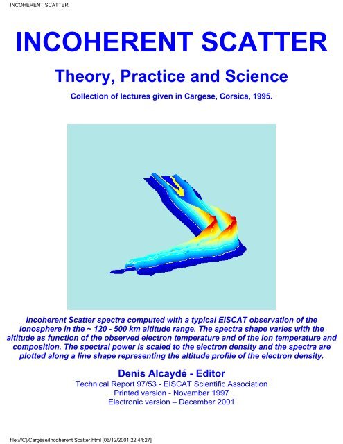
Incoherent Scatter spectra computed with a typical EISCAT observation of the 

ionosphere in the ~ 120 - 500 km altitude range. The spectra shape varies with the 

altitude as function of the observed electron temperature and of the ion temperature and 

composition. The spectral power is scaled to the electron density and the spectra are 

plotted along a line shape representing the altitude profile of the electron density. 

Denis Alcaydé - Editor 

Technical Report 97/53 - EISCAT Scientific Association 

Printed version - November 1997 

Electronic version – December 2001 

file:///C|/Cargèse/Incoherent Scatter.html [06/12/2001 22:44:27]


Table of Contents 

Author's Vademecum ii 

Editor's Foreword iii 

Acknowledgements iv 

Tor Hagfors 

Plasma Fluctuations Excited by Charged Particle Motion and their 

Detection by Weak Scattering of Radio Waves 

Wlodek Kofman 

Plasma Instabilities and their Observations with the Incoherent 

Scatter Technique 

Asko Huuskonen and Markku Lehtinen 

Modulation of Radiowaves for Sounding the Ionosphere: Theory and 

Applications 

Kristian Schlegel 

The Use of Incoherent Scatter Data in Ionospheric and Plasma 

Research 

Mike Lockwood 

Solar Wind - Magnetosphere Coupling 

Yoshuke Kamide 

Aurora/Substorm Studies with Incoherent-Scatter Radars 

Arthur D. Richmond 

Ionosphere-Thermosphere Interactions at High Latitudes 

Jürgen Röttger 

Radar Observations of the Middle and Lower Atmosphere 

file:///C|/Cargese/Table of Content.html (1 sur 4) [13/12/2001 17:27:02] 

1 

33 

67 

89 

121 

187 

227 

263


Vademecum: 

Denis Alcaydé, Dr. (Editor) Denis.Alcayde@cesr.fr 

Centre d'Etude Spatiale des Rayonnements 

F-31028 Toulouse Cedex 4 - France 

Tor Hagfors, Prof.: Hagfors@linmpi.mpg.de 

Max Planck Institut für Aeronomie - Postfach 20 

D-37189 Katlenburg-Lindau - Germany 

Asko Huuskonen, Dr.: Asko.Huuskonen@fmi.fi 

Finnish Meteorological Institute 

Helsinki - Finland 

Yoshuke Kamide, Dr.: Kamide@stelab.nagoya-u.ac.jp 

Solar Terrestrial Environment Laboratory 

Nagoya University - Toyogawa-Aichi 442 - Japan 

Wlodek Kofman, Dr.: Wlodek.Kofman@Obs.ujf-grenoble.fr 

Laboratoire de Planétologie de Grenoble 

122 rue de la Houille Blanche - F-38041 - Grenoble - France 

Markku Lehtinen, Dr.: Markku.Lehtinen@sgo.fi 

Sodankylä Geophysical Observatory 

University of Oulu - Sodankylä - Finland 

Mike Lockwood, Prof.: M.Lockwood@rl.ac.uk 

Rutherford Appleton Laboratory 

Chilton-Didcot - OX11 0QX - UK 

Arthur D. Richmond, Dr.: Richmond@ucar.edu 

High Altitude Observatory - NCAR 

Boulder - Colorado - 80307-3000 - USA 

Jürgen Röttger, Dr.: Roettger@linmpi.mpg.de 



Kristian Schlegel, Prof.: Schlegel@linmpi.mpg.de 



file:///C|/Cargese/Table of Content.html (2 sur 4) [13/12/2001 17:27:02]


Editor's Foreword 

The idea of this book came with the necessity of organising an introductory 

series of lectures for welcoming the Japanese Scientists to the European 

Incoherent Scatter Association. Indeed, after nearly 15 years of EISCAT 

operations, incoherent scatter theory, technique, practice and science have 

significantly changed, new radars have been constructed (EISCAT-ESR) and 

are planned for the future (the Polar Cap Radar project). Thus, in conjunction 

with the VIIth EISCAT Workshop organised in Cargese (Corsica-France) in fall 

1995, a series of lectures were invited and given before the Workshop 

holding: this book reflects most of these given lectures. 

This book is intended for use by graduate students for entering the field of 

Incoherent Scatter Research; it is felt however (and also hoped) that the 

various chapters of this book can be of some interest for more senior 

scientists. The book organisation is such that one can find at the beginning 

the main theoretical aspects of the Incoherent Scattering, followed by 

practical considerations on signal modulation, echoes and data analysis, and 

then scientific application aspects: 

● the first two chapters deal with the theoretical descriptions of scattering 

of plasma waves by the ionospheric plasma; Chapter one (Tor Hagfors) 

describes the "classical" Incoherent Scattering, while Chapter two 

(Wlodek Kofman) introduces the non thermal and instabilities effects. 

● in Chapter three (Asko Huuskonen and Markku Lehtinen) are introduced 

the basics of the modulation of the radio waves for pulsed radars. Once 

ionospheric echoes are received, some analysis can be made which lies 

upon some basic physics described in Chapter four (Kristian Schlegel). 

● the Solar Wind Magnetosphere interaction, Auroras and their 

ionospheric effects, Thermospheric Physics and the contributions made 

(or foreseen) by the Incoherent Scatter Observations are described in 

the following three Chapters (Chapter five, Mike Lockwood; Chapter six, 

Yoshuke Kamide and Chapter seven, Arthur Richmond, respectively). 

● the final Chapter (Chapter eight, Jürgen Röttger) deals with the theory, 

technique and science achieved with atmospheric backscatter and 

reflection processes of radio waves. 

The Editor has tried to keep as much uniformity as possible trough the 

various styles of the Authors. Notes in the text and references are printed in 

italics. The scalar symbols are in italic, the vectors are in boldface and the 

tensors (or matrices) are underlined and bold. 



Acknowledgements: 

The Editor is happy to thank all the Authors who very hardly worked for 

producing a written version of their Cargese lecture; all Authors have kindly 

provided the Editor with almost all the necessary materials (texts, equations 

and figures) close to their final form, thus making the Editor work much 

simplified. 

The Editor would like also to deeply acknowledge the Director of EISCAT, Dr. 

Jürgen Röttger, who have accepted to use the "EISCAT-Technical Reports" 

series as the practical printing, publishing and distribution of the book. 

Thanks are also given to several colleagues who have, in the CESR, "peu ou 

prou" contributed to the final edition of the book, and finally to Anette Snallfot 

in EISCAT-HQ who has so kindly helped and served as the intermediate 

between the Publisher and the Editor. 

This Editor's work has been made possible through partial funding of the GdR 

Plasmae of CNRS. 

EISCAT is an international association, supported the research councils of 

Finland, France, Germany, Japan, Norway, Sweden and the United Kingdom. 

Denis Alcaydé - November 1997 

Electronic version – December 2001 


PLASMA FLUCTUATIONS EXCITED BY CHARGED PARTICLE 

MOTION AND THEIR DETECTION BY WEAK SCATTERING OF 

RADIO WAVES 

Tor Hagfors 

1. Introduction 

If spatial fluctuations or variations in refractive index exist in a medium a wave 

cannot propagate through it unperturbed because energy will be scattered by the refractive 

index variations into other directions. In most cases the spatial fluctuations 

are also time dependent, and the time variation of the scattered wave will no longer 

be the same as that of the unperturbed wave. Such phenomena have been studied in 

many branches of physics, notably in connection with tropospheric and ionospheric 

scattering of radio waves by irregularities caused by turbulence. In the latter case the 

density fluctuations are caused through the action of external macroscopic sources. 

The fluctuations that we are about to discuss in the present paper are caused by the 

fact that the plasma is built of discreet charged particles. When these particles are 

moving through the plasma they will excite electron density fluctuations which can 

be detected by electromagnetic wave scattering. This is the type of scattering which 

has become known as "incoherent scattering". 

There is available a large number of papers dealing with the theory of incoherent 

scattering of radio waves, particularly with reference to the ionosphere. [Gordon, 

1958; Fejer, 1960; Dougherty and Farley, 1960; Salpeter, 1960; Renau 1960; Hagfors, 

1961; Rosenbluth and Rostoker, 1962]. Later important additional contributions 

have been made by Woodman [1965], Moorcroft [1964] and Perkins et al. [1965]. 

Rather complete discussions of the subject matter have been given by Sitenko [1967] 

and by Sheffield [1975]. 

The observations made over the last decades have shown that incoherent scattering 

has become one of the most fruitful methods of investigating the ionosphere to 

heights of several thousand kilometres from the ground. [Bowles, 1958; Pineo et al., 

1960; Millman et al., 1961; Bowles et al., 1962]. Excellent reviews of the experimental 

work have been given by Evans [1968] and Beynon and Williams [1978] 

The method is particularly useful because in addition to providing data on 

electron density it is also capable of giving information on parameters such as 

electron and ion temperatures, the ionic composition, or the orientation of the 

magnetic field. The extension of routine measurements to include the region above 

the peak of the ionosphere is of great importance to the understanding of 

1

the behaviour of the ionospheric layers. It is interesting that incoherent scattering has 

also found application as a diagnostic tool for hot plasmas in thermonuclear research 

following the development of practical laser sources. [Rosenbluth and Rostoker, 

1962]. 

The first suggestion that incoherent scattering might be used to measure electron 

density in the ionosphere was made by Gordon [1958]. Gordon estimated the total 

scattered power by adding powers scattered by individual electrons and concluded 

that present day radars had sufficient sensitivity. He also inferred that the waves 

scattered by the plasma would be subject to Doppler broadening, and predicted the 

amount of broadening by adding power scattered by individual electrons travelling 

with velocities corresponding to a Maxwellian velocity distribution. The first observations 

by Bowles [1958] showed that the predicted spectral broadening in particular 

was seriously in error. 

Subsequent theoretical work explained the discrepancy as due to neglect of particle 

interactions in the original theory. It was shown that the width of the broadened 

lines should correspond with the thermal speed of the ions rather than that of the 

electrons. The total power scattered was shown to be less than predicted by Gordon 

by a factor of 1/2 in most cases of interest provided ions and electrons are at the 

same temperature. For hot electrons and cold ions - a situation which often prevails 

in the ionosphere - the power is often less than this [Buneman, 1962]. 

When an external magnetic field is included in the considerations additional complications 

arise. Bowles [1961] suggested that spectral distributions might contain 

lines corresponding to ionic gyro resonances. This suggestion has been confirmed 

theoretically, and the conditions have been given under which ion lines might be observed, 

[Salpeter, 1961; Hagfors, 1961; Farley et al., 1961; Fejer, 1961]. 

It appears that the theoretical analysis - i.e. the first order analysis - is more or less 

complete in that several workers have arrived at identical or nearly identical conclusions 

based on widely different approaches. In all results, however, with the exception 

of that of Farleyet al. [1961], the excitation of hydromagnetic waves by the microscopic 

motions is missing. Discussions of the interaction with transverse modes 

have also been given by Sitenko [1967] and by Sheffield [1975]. In most calculations 

of fluctuations only Coulomb interactions are accounted for and this seems to be 

adequate for ionospheric purposes. 

In the present paper an attempt is made to rederive the expressions for the 

scattering from first principles and fairly readily understandable pictures. This 

becomes particularly simple when we make full use of the concept of "dressed 

particles" first introduced into plasma physics by Rosenbluth and Rostoker 

2

[1962]. The gain in physical insight using the dressed particle concept is purchased 

at the cost of some rigor. 

Section 2 deals with the problem of evaluating the total scattered power and the 

spectral distribution of this power in terms of the properties of the plasma. A general 

discussion is then given in Section 3 of the various factors determining these properties 

of the plasma, beginning with a plasma of noninteracting particles, with or without 

an external magnetic field, proceeding with the effect of paricle interaction in the 

form of collective electrostatic interaction, and ending up with power spectra of the 

fluctuations under various physical conditions. 

2. The Relationship of Scattering to Electron Density Fluctuations 

We first compute the power reradiated by a certain volume V of a plasma which is 

irradiated by a plane monochromatic wave with wave vector N at a frequency ω 

much higher than the plasma frequency for electrons ω pe defined by: 

ωpe = 

⎩⎪ ⎨⎪⎧ n0 q 2 

e 

where: 

⎪⎫ 1/2 

⎬ 

m ε0 ⎭⎪ 

n 0 = electron density 

q e = electron charge 

m = mass of an electron 

ε 0 = dielectric constant of free space. 

Rationalized MKSA units will be adhered to throughout. 

The field scattered by a single electron within the volume V, see Figure 1, will 

then be: 

E p = E in exp{ i (ω 0 t -N .r p(t)} 1 

R 0 exp{-i ω 0 

c R 0 } σ 0 exp{ i K.r p (t) } (2) 

Here r(t) is the position of the particle at time t and σ 0 is the effective scattering "radius" 

of the electron defined by: 

q e 2 

σ0 = r0 sinχ = ⎜ 

⎝ ⎜⎛ 

4π ε0 ⎞ 

⎟ 

⎟ 

⎠ 

3 

(1) 

1 

m c2 sinχ (3)

Figure 1. Scattering from electron at position r p (t). 

where χ is the angle between the electric field vector of the incident wave and K, i.e. 

the direction toward the observer. Certain complications might arise through the 

presence of an external magnetic field, but these will not be considered here. 

We see that the scattering is determined by the difference of the wave vectors of 

the incident and the scattered waves, k = N - K. On the assumptions of weak scattering 

the total field at the observer becomes: 

E obs = E in σ 0 

R 0 exp ⎩ ⎨ ⎧ 

i (ω 0 t - ω 0 

⎫ 

⎬ 

c ⎭ 

) R ∑ 0 

p 

4 

exp {-i k.r p (t)} (4) 

where the summation is extended over all the electrons within the volume V. 

It will prove convenient to express the scattered field in terms of electron density 

n(r,t). Because electrons are here considered as point particles the number density is 

most easily expressed as a sum of δ-functions in space: 

n(r,t) = ∑ p 

δ {r - r p (t)} (5) 

We now expand in spatial Fourier series within a periodicity cube of volume V:

n(r,t) = ∑ k 

with: 

n (k,t) . e i k.r (6 a) 

n (k,t) = 1 

V ⌡ ⎮⌠ 

d(r) n(r,t) e i k.r (6 b) 

The observed field E obs can therefore be expressed as: 

E obs = σ 0 

R 0 E in . V . n(k,t) exp{ -i ( ω 0 t - ω 0 

c R 0 )} (7) 

It follows from this result that the signal observed at the receiver with a plane 

monochromatic wave incident on the volume V has the character of a modulated signal 

centred on the carrier frequency ω 0 [approximately !] and with complex amplitude 

proportional to n(k,t), k being the wave vector difference as introduced above. 

The complex amplitude hence becomes: 

A obs (t) = σ 0 

R 0 E in v . n(k,t) (8) 

The statistical properties of the complex amplitude at the receiver are therefore the 

same as those of n(k,t). The received signal is conveniently described statistically by 

the autocovariance: 

〈 A *(t) A(t + τ) 〉 av 

and the power spectrum is found by Wiener - Khinchine’s theorem as the Fourier 

transform of this: 

P obs (ω) = σ 0 2 

R 0 2 E in 2 . N . φ (k,ω) = N . P T .φ (k,ω) (10) 

where P T is the total power scattered by a single electron under the same geometrical 

conditions, N is the total number of electrons in the volume V and φ (k,ω) is the Fourier 

transform of the autocorrelation function of electron density fluctuations: 

ρ(k,τ) = V2 

N 〈 n*(k,t) n(k,t + τ) 〉 av 

5 

(9) 

(11)

Figure 2. Geometry of incident and scattered waves. 

Note that the omission of the exponential time variation exp{i ω 0 t} has shifted the 

power spectrum of the received signal P obs(ω) down to zero frequency. The frequency 

ω from now on only corresponds to the amount of Doppler displacement 

from the transmitted frequency ω 0. 

Physically we may visualize the scattering to occur as follows: at any given time 

there is present in the scattering volume electron density waves travelling in all different 

directions with all different wavelengths. The transmitter-receiver geometry 

represented by the wave vectors N and k picks out one particular of these "waves" as 

responsible for the scattering. With a scattering angle ϕ, see Figure 2, the wavelength 

of these density waves is: 

Λ dens = 

λ 

2 sin (ϕ / 2) 

where λ is the radio wavelength. The strong resemblance of this formula with the 

condition for reflection in a crystal lattice given by Bragg should be observed [Figure 

2]. 

Doppler shift ω now corresponds to motion of our particular density variation. For 

each velocity there is a corresponding Doppler frequency ω . The velocity v, positive 

along positive k, is related to the Doppler shift frequency ω through: 

v = λdens . ω ω . λ ω 

= - 

= - 

2π 4π sin (ϕ / 2) |k| 

6 

(12) 

(13)

With this discussion the whole problem of the scattering process has been tied to 

properties of the plasma and density fluctuations therein. Such fluctuations are studied 

in detail in the following sections. 

3. Electron Density Fluctuations 

In the discussions to follow we neglect the effect of binary collisions on the density 

fluctuations. This is a good approximation in a sufficiently dilute plasma such as 

the upper part of the ionosphere, where collective interactions tend to dominate. In 

the first of the subsections to follow we also neglect long range interactions, and 

consequently begin our considerations with a gas of non-interacting particles. Such a 

gas will lack many of the familiar properties of gases - for instance it will be unable 

to support ordinary sound waves. A discussion of such a peculiar plasma is nevertheless 

useful; because, as will be shown later on, a plasma with particles interacting 

through electromagnetic fields will in first order behave as if the particles move independently, 

but with a cloud of charge surrounding them - as if "dressed". 

The random thermal motion of individual particles will represent charge and current 

fluctuations due simply to the discreetness of the particles. This is a sort of "intrinsic 

fluctuation" associated with the atomicity of the gas. When in the second subsection 

we go on to consider electromagnetic field interactions it will be shown that 

the interaction fields can be regarded as excited by the charge and current fluctuations 

caused by the thermal motion of individual particles. These fields in turn will 

induce fluctuations in the plasma, and these "induced fluctuations" are superimposed 

on the intrinsic fluctuations caused directly by the discreet nature of the particles. 

The discussion will allow non-equilibrium situations to prevail, although the distributions 

must be stationary in the Vlasov sense. Most formulae actually given explicitly 

will apply to a quasiequilibrium situation where electrons and ions are separately 

in equilibrium but not necessarily at the same temperature. Whenever explicit calculations 

are carried out the velocity distributions will be taken as Maxwellian. 

3.1. Fluctuations in a Gas of Non-Interacting Particles 

We consider the motion of charged particles in rotating coordinates defined as 

follows: 

⎛ 

⎜ 

⎜ 

⎜ 

⎝ 

Cartesian: Rotating: 

r = {x,y,z} r1 = 1 

(x + i y) 

2 

r-1 = 1 

(x - i y) 

2 

r0 = z 

⎞ 

⎟ 

⎟ 

⎟ 

⎠ 

7 

(14)

Here the z-axis which is the axis of symmetry coincides with the direction of the 

external magnetic field B 0. From Eq. 14 it is obvious that there is a unitary transformation 

between Cartesian and rotating coordinate systems. For the equation of motion 

of a single particle we obtain: 

v . α = - i q B 0 

m α v a = - i α Ω v a (α = 1, -1, 0) (15) 

For the time being we allow the gyrofrequency Ω to be negative for electrons and 

positive for ions. This brings out the real advantage in using rotating coordinates: the 

equations of motion are diagonalized. 

If at the present time t the velocity and position of the particle are v (t) = {v +1;v - 

1;v 0} and r (t) = {r +1;r -1;r 0} then the particle velocity and position at an earlier time 

t’ must have been: 

v α (t') = v α (t - τ) = v α (t) . e i α Ω t (16 a) 

Or in vector form: 

v(t - τ) = Γ . (τ) v(t) (16 b) 

where Γ . (τ) is a matrix transforming from present to past velocities. In polarised coordinates 

the matrix is on diagonal form. Similarly past and present particle positions 

are related through: 

r α(t - τ) = r α(t) - ei α Ω t - 1 

i α Ω v α(t) (17 a) 

or again in vector form: 

r(t - τ) = r(t) - Γ(τ) v(t) (17 b) 

Γ (τ) transforming from present to past position is also on diagonal form in our 

coordinate system. The elements of the matrices describing the screw motion of the 

particles are: 

Γ . 

αα = g . α = e i α Ω t (18) 

and 

Γ αα = g αα = ei α Ω t - 1 

i α Ω (19) 

8

In Section 2 we saw that each particle contributes an amount 

n p (k,t) = 1 

V e-i k.rp(t) (20) 

to the Fourier transform of the particle density giving rise to the scattering. The complex 

autocorrelation in particle density associated with a single particle becomes: 

〈 n p *( k, t) n p( k, t+τ)〉 av = 〈 n p *( k, t-τ) n p ( k, t)〉 av = 

1 

V2 〈 e(-i k-α gα vα )〉 av = (21) 

1 

V2 ⌡ ⎮⌠ d(v) fo(v) e -i a.v 

Here f 0(v) is the velocity distribution of the particles and a is a vector defined by: 

a -α = k -α g α = k -α e i Ω α τ -1 

i Ω α (22) 

The complex autocorrelation function normalized as in Eq. 11 becomes: 

ρ (k,τ) = 〈 e -i a.v 〉 av 

The correlation function for density fluctuations in a gas of non-interacting particles 

is therefore a function of the vector a and of the parameters of the single particle 

velocity distribution. 

The Fourier component of single particle current density similarly becomes: 

9 

(23) 

j p (t) = q 

V v p (t) e -i k.rp(t) (24) 

A statistical description of this random current is provided by the autocovariance 

of the rotating components of the current: 

〈 j µ * ( k, t) j ν * ( k, t+τ)〉 av = 〈 j µ * ( k, t-τ) j ν * ( k, t)〉 av= 

q 2 

V 2 g. -µ ⎝ ⎜ ⎛ 

- 

∂ 2 

⎞ 

⎟ 

⎠ 

∂ a µ ∂ a ν ρ (k,τ) (25) 

Because of the independency of the particles the expression for the total current is 

obtained by multiplication by N, the total number of particles.

The normalized autocorrelation function ρ (k,τ) thus enters both in the determination 

of current and charge density fluctuations. Before giving a specific form for 

f 0(v) and hence for ρ (k,τ) it is worthwhile to discuss in a rather qualitative manner 

some of the properties of this function, or its Fourier transform which is the power 

spectrum. 

As was explained in Section 2 the density fluctuations can be thought of as a superposition 

of density waves travelling in all different directions with all different 

velocities and wavelengths. Suppose first the k is along the magnetic field. The particle 

motion in this direction is independent of the field and we expect the density 

fluctuations to be the same as if no magnetic field were present. 

The density waves are carried along k by beams of particles with thermal velocities 

equal to the wave velocities, and with amplitudes proportional to the number of 

particles in the beams. Because the number of particles in each beam specified by the 

velocity v = ω/k is proportional to f 0(v //) the power spectrum in this case is just proportional 

to the velocity distribution along the magnetic field with v // replaced by 

(ω/k). The autocorrelation ρ (k,τ) is the Fourier transform of this power spectrum. 

Figure 3. Typical particle trajectory shown in relation to a density wave . Transverse case, β = 90°, 

large Larmor radius. 

10

At the other extreme, that of k perpendicular to B 0 the density waves are travelling 

at right angles to the field. In Figure 3 the magnetic field is along the z-axis and the 

waves are travelling in the x-direction. Furthermore the radius of gyration, or the 

Larmor radius defined by: 

R = 2 v th 

Ω (26) 

[where v th is the r.m.s. thermal velocity] is large compared with the density wavelength. 

Suppose the particle density projected into the x-y plane at t = 0 is of the 

form shown to the extreme left. Redistribution of particles along the x = constant 

plane will have no influence on the density component under consideration. If we 

pick out any straight line parallel to the magnetic field characterized by x 0y 0 the particles 

leaving this line with any velocity in any direction will return to this line after 

exactly one period of gyration T = 2π/Ω. The density will therefore be a repetitive 

time function with period T, and this periodicity must also appear in the autocorrelation 

function. 

In the example shown in Figure 3 the radius of gyration of a thermal particle is 

large compared with the wavelength of the density waves and the particles can travel 

along with the density wave at least for a few wavelengths before being bent away 

from the direction of the wave. Had we chosen the radius small compared with the 

wavelength of the density variation, the time variation would lose the character of a 

wave phenomen because the particles would be so strongly attached to the magnetic 

field lines that they would no longer be able to transport a spatial variation along k 

by even as little as one wavelength. 

The spatial variation would then tend to appear as a nearly stationary pattern, and 

the power spectrum would be extremely [Figure 3] narrow. In the autocorrelation 

picture a small Larmor radius, i.e. a strong magnetic field, would give an autocorrelation 

function close to unity for all time shifts τ. The periodic modulation of ρ (k,τ) 

so prominent for large Larmor radii would be rather shallow in this case.In scattering 

of radio waves from the ionosphere at frequencies less than about 1000 MHz the 

Larmor radius of electrons will be small and that of the ions large compared with the 

density scale of interest, i.e. Λ dens = λ / 2 sin(ϕ / 2). 

As we have just seen there is no effect of a magnetic field in the longitudinal case 

[β = 0°] but there is a profound effect for the transverse case [β = 90°]. Let us now 

examine what happens in the intermediate range. We start by letting decrease β 

slightly from 90°. 

As long as β is exactly 90° motion of the particles along the magnetic field does 

not matter because this only corresponds to motion along planes of constant 

11

phase of the density waves. As soon as the perpendicularity condition is relaxed, 

motion along the field does indeed matter, because when the particle gyrates once 

round the field line that it left T seconds earlier, it might at the same time have slid 

along the field line to such an extent that it no longer fits into the original phase relationship 

with the density wave. In the case of large Larmor radius the condition for 

spectral lines to occur in the power spectrum can be found by considering Figure 4. 

The projection is here shown of a typical particle trajectory into a plane containing 

the magnetic field B 0 and the propagation vector k. The typical velocity along the 

magnetic field is v th where v th is the thermal velocity in the z-direction. The typical 

distance of motion of this particle along the magnetic field during one period of gyration 

becomes: 

1 = vth .T = vth . 2π 

Ω = 2 R . 2 . vth = 2 π . R (27) 

Ω 

where R is again the Larmor radius as defined in Eq. 26. The motion of the particle 

along the wave normal k during the same time becomes: 

∆ s = 1 . cos β = 2 π R cos β = 2 π R sin ψ (28) 

Now, if the motion of the particle along the field line during one period of gyration 

has caused the particle to get out of step, or out of phase with the density variation, 

then the deep periodic modulation of the autocorrelation function will disappear. 

For large Larmor radii the condition for the magnetic field to have an appreciable 

influence on the spectrum becomes: 

Figure 4. Particle trajectory in relation to a density wave for arbitrary β. 

12

k . ∆ s < π 

2 

or: sin ψ < 

1 

2 2 k R 

which is the condition for the particle to keep in phase with the density variation for 

at least one period of gyration. 

For small Larmor radii the modulation of the spectrum is never very prominent. In 

passing from β = 90° to β = 0° the autocorrelation function will just gradually shrink 

from being close to unity for all τ at β = 90° to the no-magnetic field case at β = 0°. 

The spectrum will therefore be narrow when β = 90° and identical with the nomagnetic 

field case at β = 0° with a gradual transition between the two cases. This is 

easily understood by considering the particles as completely constrained to move 

along the field lines. The r.m.s. motion along the direction of k - and this is the component 

of motion giving rise to the spectral broadening - is then simply: 

13 

(29) 

v k = v th . sin ψ (30) 

and the width of the power spectrum is just proportional to v th 2 sin 2 ψ = v th 2 cos2 β. 

In order to check the rather intuitive conclusions regarding the properties of 

ρ (k,τ) this function was evaluated for a Maxwellian velocity distribution: 

f0 (v) = ⎜ 

⎝ ⎛ 2π 

⎞ 

⎟ 

v 2 

th ⎠ 

3/2 

e -v2 /2vth 2 (31) 

where v th is the r.m.s. thermal velocity defined by: 

v th 2 = θ / m θ being the absolute temperature, in energy units. 

The result is: 

ρ (k,τ) = e {-½ v th 2 |a|2 } =e -(kR) 2 {(½Ωτ)2 cos2 β + sin 2 (½Ωτ p ) sin 2 β} 

This result is plotted on a log-linear diagram in Figure 5, correlation against normalized 

time shift Ωτ/2π = τ/T [T = time of gyration] with the angle β as parameter. 

It will be seen from Figure 5 that the autocorrelation function exhibits exactly the 

properties arrived at by the more qualitative arguments just presented. Modulation is 

only prominent when β is close to 90° and Larmor radius large, depth of modulation 

decrease with Larmor radius. 

The integral over the spectrum Φ (k,ω) over all frequencies f, which is proportional 

to the total scattered power, is equal to ρ (k,ω). This is unity in all cases 

(32)

considered so far. Independent particles therefore scatter incoherently, i.e. the scattered 

power is obtained by adding powers scattered by individual particles. The effect 

of magnetic field is to redistribute the power whilst all the time keeping the total 

scattered power constant. 

The actual spectral function Φ (k,ω) becomes: 

Φ (k,ω) = Re 

⎪⎧ 

⎨ 

⎩⎪ 

∞ 

⌠ 

⎮ 

⌡ 

-∞ 

⎪⎫ 

⎬ 

⎭⎪ 

ρ(k,τ) e- iωτ dτ (33) 

because ρ (k,τ) will be assumed to be real and symmetric in τ. When steady drifts are 

superimposed this is no longer the case and the spectrum must be obtained with some 

care. For the Maxwellian velocity distribution the spectrum becomes: 

Φ(k,ω) = 2 ⌡ ⎮ ⌠ 

0 

∞ 

e-½ v th 2 |a| 2 cos ωτ dτ (34) 

Figure 5. Autocorrelation of independent particle number density [logarithmic scale] versus normalized 

time shift [ωτ/2π] with angle β as parameter. 

14

For later purposes we define the function 

G(k,ω) = ⌡ ⎮ ⌠ 

0 

∞ 

e-½ v th 2 |a| 2 - iωτ dτ (35) 

and term it a Gordeyev integral. In terms of this function the spectrum may be expressed 

as: 

Φ(k,ω) = 2 Re {G(k,ω)} (36) 

3.2. The Effect of a Random Electric Field 

With electromagnetic particle interaction present the motion of individual particles 

becomes more complicated because each particle moves in the field of all the others. 

In this subsection we want to determine the density variations induced by the interaction 

field. Such density variations come in addition to the density fluctuations 

caused by the discreetness of the particles, i.e. the intrinsic fluctuation dealt with 

above. The induced fluctuations may be computed as if the particles were smeared 

out into a continuum. The fields giving rise to these induced fluctuations must, however, 

be computed from the discreet particle picture of the non-interacting gas. From 

this we realize that there are two contributions to the density fluctuations, one from 

the discreetness of the particles, the intrinsic part, and another one due to fluctuations 

induced by the fields - which in turn are caused by the discreetness of the charged 

particles. A charged particle moving through the plasma in itself constitutes a fluctuation, 

but in addition it induces a fluctuation in the surrounding medium due to the 

fields it sets up. The particle plus the charge cloud surrounding it is often referred to 

as a "dressed particle" [Rosenbluth and Rostoker, 1962]. 

Assume first that the force per unit mass is known throughout the plasma, and let 

this force be denoted by F(r,t). The density fluctuation induced by this force in a 

volume element having velocity v at position r at time t is then found from the Vlasov 

equation to be: 

δ n (r,v,t) = - n 0 ⌡ ⎮ ⌠ 

-∞ 

t 

F(r’,t’) . ∂ f0 (v’) 

∂v’ 

dt’ (37) 

The integration is extended over the orbit of the volume element at all earlier 

times. If the unperturbed velocity distribution f 0(v) is isotropic the force F(r,t) can be 

expressed as q E(r,t) where E is the internal electric field caused by the 

15

discreetness of the particles. The magnetic force vanishes because under the isotropy 

assumption this force is perpendicular to [∂ f0 / ∂ v]. The presence of externally applied 

fields can always be accounted for in the computation of individual particle 

orbits. With a Maxwellian velocity distribution we obtain: 

δ n(r,v,t) = n 0 q 

mv th 2 ⌡ ⎮⌠ 

∞ 

t 

E(r’,t’) . v’ f 0(v’) dt’ (38) 

Physically this corresponds to the energy acquired by the volume element arriving 

at r at time t with velocity v from the electric field divided by the mean energy of a 

thermal particle. The integration is along actual particle orbits. If the fluctuating field 

is rather small the perturbation in particle orbits due to the random field will be 

small, and the integration can be carried along orbits which are unperturbed by the 

random field. Relations between past and present velocities and positions are therefore 

the same as in a gas of noninteracting particles as studied in the previous section. 

In this study we are interested in spatial fluctuations irrespective of the velocity of 

arrival v and we therefore average over all velocities of arrival making use of the fact 

that f 0(v) = f 0(v’) for unperturbed orbits, and obtain: 

δ n(r,t) = n 0 q 

mv th 2 ⌡ ⎮⌠ 

d(v) f 0(v) ⌡ ⎮ ⌠ 

-∞ 

t 

E(r’,t’) dt’ (39) 

We next expand the electric field E(r’,t’) in a spatial Fourier series: 

E(r’,t’) = ∑ k 

E(k,t’) e ik.r’ (40) 

Putting t’ = t - τ and making use of the relations between past and present positions 

derived in Section 3.1 we obtain: 

δ n(r,t) = n 0 q 

mv th 2 ∑ k 

e ik.r 

∞ 

⌠ 

⎮ 

⌡ 

0 

dτ E(k,t-τ) ⌡ ⎮⌠ d(v) f0(v) Γ . (τ) v e-ikΓ(t)v (41) 

16

It follows that the spatial Fourier components of the field induced fluctuation become: 

n 1 (k,t) = n 0 q 

mv 2 

th ⌡ ⎮⌠ dτ T(k,τ) . E(k,t-τ) (42) 

0 

∞ 

where we have introduced a vector T(k,τ) with rotating components: 

Ta (k,τ) = ⎮ 

⌡ ⌠ 

d(v) f0(v) g . a(τ) va e-ia.v = g . a(τ) ⎜ 

⎝ ⎛ 

17 

i ∂ 

∂ a -a 

⎞ 

⎟ 

⎠ 

ρ(k,τ) (43) 

where a is again the vector defined in Eq. 22, and where ρ(k,τ) is the autocorrelation 

function of density fluctuations of non-interacting particles. 

Equation 42 should be compared with the equation relating the current density and 

the electric field in a dispersive medium: 

j (k,t) = ⌡ ⎮ ⌠ 

0 

∞ 

dτ σ(k,τ) E(k,t-τ) (44) 

where σ(k,τ) is the conductivity tensor of the medium. We might say that σ(k,τ) describes 

the way in which the medium responds with a current to an applied electric 

field. In the same way we might interpret the vector (n 0 q)/(mv th 2) T(k,τ) as describing 

the way in which the medium responds with a density variation to an applied 

electric field. 

The superscript "1" will henceforth be used to signify the field-induced fluctuation 

as distinguished from the intrinsic fluctuation which henceforth will be labelled by 

superscript "0". The total fluctuation in the plasma now becomes: 

n(k,t) = n 0 (k,t) + n 1 (k,t) (45) 

As the field E and the response vector T appear as a one-sided convolution integral 

it will be more convenient to work in the frequency domain. In this way we determine 

power spectra directly without going via the autocorrelation function which 

proved so convenient in the description of a gas of non-interacting particles. For the 

induced fluctuation we obtain: 

n 1 (k,ω) = E(k,ω) T(k,ω) ⎝ ⎜ ⎛ 

n0 q ⎞ 

⎟ 

mv 2 

th ⎠ 

(46)

We must be careful in defining T(k,ω) - it is a one-sided Fourier transform: 

T(k,ω) = ⌡ ⎮ ⌠ 

0 

∞ 

T(k,τ) e-iωτ dτ (47) 

This is due to the one-sided convolusion which in turn is caused by the fact that only 

the past not the future can determine the fluctuation at the present time. 

The field E(k,ω) is a superposition of the fields from the individual particles of the 

plasma. If we compute the field from one particular particle we will be able to determine 

the fluctuation induced by this particle alone. Let this induced one-particle 

fluctuation be denoted by n p 1(k,ω). Suppose we are interested in electron density 

fluctuations. The contribution to these from a particular electron p becomes: 

np (k,ω) = n 0 

p (k,ω) + ⎜ 

⎝ ⎛ n0 q ⎞ 

⎟ 

mv 2 

th Epe (k,ω).Te (k,ω) (48) 

⎠ 

where n p 0 (k,ω) is the intrinsic fluctuation associated with electron p. In the second 

term which represents induced fluctuation, the electric field E pe (k,ω) is that associated 

with particle p only. The intrinsic term may thus be associated with the "bare" 

particle and the second term with the "dressing" surrounding the particle - on the average 

an electron repels other electrons thus creating an electron deficiency in its 

neighbourhood. In addition to the "electron dressing"the electron will also be accompanied 

by an "ion dressing" due to the average attraction of ions by the electron. 

For a Maxwellian velocity distribution the components of T(k,ω) can be determined 

by means of Gordeyev integrals: 

G(k,ω - αΩ) - G(k,ω) 

Ta (k,ω) = - v 2 

th . ka α Ω 

For α = 0 or when ω → 0 we must take the limit of this which does not exist. For 

α = 0 we have: 

T 0 (k,ω) = v th 2 . k 0 . 

18 

(49) 

∂ G(k,ω) 

∂ ω (50)

We see that, when ω → 0 the vector T(k,ω) becomes parallel to the vector k. This 

means that the only component of the electric field which can induce fluctuations is 

that along k, i.e. E L defined by: 

EL = 1 

k2 k (k .E) (51) 

As this component of the field is determined by the charge fluctuations alone it 

means that the Coulomb interaction approximation is no approximation at all but an 

exact solution of the first order fluctuation problem in this particular case. 

An ion can of course only contribute to electron density fluctuations through an 

induced fluctuation, or, if we like, through its electron "dressing". The electron density 

fluctuation associated with an ion p is therefore: 

n p(k,ω) = n 0 q e 

mv th 2 E pi (k,ω) . T e (k,ω) (52) 

where E pi (k,ω) is the field induced by the particular ion p. 

Once these elementary contributions have been determined the total electron density 

fluctuation can be found as a superposition of contributions from all the "dressed 

electrons" plus all the ion "dressings": 

〈|n(k,ω)| 2〉 av = contribution from "dressed electrons" 

+ contribution from ion "dressings". 

Before further progress can be made we must calculate the electric field set up in 

the plasma as a result of the motion of a charged particle along an unperturbed orbit. 

As most calculations of this electric field in connection with plasma fluctuations tacitly 

assume the longitudinal interaction [= Coulomb interaction] to be the only form 

of interaction,we shall devote the next subsection to the calculation of this field. 

3.3. The Effective Field of a Charged Particle Moving Through the 

Plasma 

The inducing electric field Ep(k,ω) associated with the motion of a charged particle 

may be calculated by solving Maxwell’s equations in vacuo by a Fourier transform 

in space and time assuming the field to be excited by a current jp(k,ω) which 

consists of two terms, one is the driving or intrinsic term j 0(k,ω) p caused directly by 

the motion of the discreet particle - this is identical with the current studied in Section 

3.1 - and the other term is an induced current caused by the field set up. 

19

We now imagine the field E p(k,ω) to be split in a longitudinal part E L [see Eq. 51] 

and a transverse part E T (k,ω) defined as: 

ET (k,ω) = - 1 

k2 (k x (k x E)) (53) 

Here we shall consider only the longitudinal interaction. This is exactly correct 

when there is no magnetic field so that the transverse and the longitudinal modes decouple 

exactly. When there is a magnetic field present there is a coupling, but the 

transverse field in general only becomes important for such small values of k that it 

is of no interest in scattering from the ionosphere. We obtain: 

n 1 p(k,ω) = n 0 q e 

mv th 2 E T . T = n 0 q e 

k 2mv th 2 [ k.E p(k,ω) ] [ k.T 0(k,ω)] (54) 

and the scalar product k.E p (k,ω) can be related directly to the charge density fluctuation 

associated with the motion of a particle p. If this particle is an electron, the 

charge density fluctuation becomes: 

ρ pe (k,ω) = q e { n 0 p (k,ω) + n 1 p (k,ω) } + q i N 1 p (k,ω) (55) 

The last term q i N 1 p (k,ω) is the fluctuation induced by the electron p in the ion 

density. When several ionic constituents are present it must be summed over similar 

terms, one for each constituent. For simplicity we only assume one type of positive 

ions to be present, and that these have mass M, thermal velocity V th and average density 

N 0 sufficient for neutrality of the plasma as a whole. Introducing Debye lengths 

for electrons and ions we have: 

⎛ 

⎜ 

⎝ 

D 2 

e = ε0 mv 2/n th 0 q 2 

e = (vth/ωpe) 2 

D 2 

i = ε0 MV 2/N th 0 q 2 

i = (Vth/ωpi) 2 

20 

(electrons) 

(ions) 

where ω pe and ω pi are the plasma frequencies for electrons and ions respectively. 

The Debye length is therefore the distance travelled by a thermal particle during one 

period of a plasma oscillation. Combination of these quantities with Eq. 54, 56 and 

with the equation 

⎞ 

⎟ 

⎠ 

(56) 

k.E p (k,ω) = - ρ pc (k,ω) (57) 

which follows from Maxwell’s equations, gives for the longitudinal field: 

E Lp (k,ω) = 

- i k . (q e/ε 0k 2) n 0 pe (k,ω) 

1 + i {(1/kD e) 2 k.Te + (1/kD i) 2 k.T i} 

(58)

When the field-inducing particle is an ion we only have to replace q en 0 pe(k,ω) by 

the similar expression for an ion, viz. q iN 0 pL(k,ω). Replacing the expression 

i (1/kD) 2 k.T by the more commonly used longitudinal susceptibility χ = kχ t k/k 2, we 

see that the denominator in Eq. 58 enters as a dielectric constant of the plasma, and 

the field set up is a screened field. 

From these considerations we can write down directly the total fluctuation associated 

with a single electron: 

n pe (k,ω) = (1 + χ i) n 0 pe(k,ω) 

1 + χ i + χ e 

and for the electron density fluctuation induced by a single ion [assuming q e = - q i 

!]: 

n pe (k,ω) = = χ e N 0 pi(k,ω) 

1 + χ i + χ e 

The total fluctuation of electron density is obtained as a superposition of fluctuations 

from all the individual particles - now being regarded as independent. This procedure, 

which has been termed by Rosenbluth and Rostoker [1962] a "superposition 

of dressed test particles" gives the correct first order fluctuation for Coulomb interaction 

only. By inverting the above expression for electron-density fluctuation from 

k,ω space into r,t space we could study in detail the electron cloud associated with 

the motion of an ion. Fast ion motion would give a wake of electron density disturbance 

travelling away from the inducing ion. The above expression therefore represents 

the kinetic theory result of the problem of a charged particle passing through a 

plasma. It should be observed that the above expressions are valid for Coulomb interaction 

only. 

3.4. Spectral Distribution of Fluctuations 

From Eq. 59 and 60 we can now construct the spectral distributions by simple superposition 

of independent dressed particles. For electrons and one kind of positive 

ions we obtain: 

〈| n e (k,ω) | 2 〉 av = |1 + χ i| 2 〈|n 0 e (k,ω)| 2〉 + |χ e| 2 〈|N 0 i (k,ω)| 2 〉 

| 1 + χ e +χ i | 2 

where 〈|n 0 e (k,ω)| 2〉 and 〈|N 0 i (k,ω)| 2〉 are the power spectra of independent electrons 

and independent ions as studied in Section 3.1. 

21 

(59) 

(60) 

(61)

Figure 6. Characteristics of the equilibrium spectra for various Debye lengths, expressed in terms 

of X p =1/kD 

This result is identical with results derived by other workers. In our derivation of 

Eq. 61 we did make use of Maxwellian velocity distributions for ions and electrons 

to define v th. We are, however, perfectly free to prescribe a non-equilibrium situation 

with electrons and ions at different temperatures. Also, with many different types of 

ions present we only have to replace the ion terms above by a sum of such ion terms 

subject only to neutrality of the plasma as a whole. This has been carried out by 

Buneman [1961] in detail. We also observe that by starting with a non-Maxwellian 

velocity distribution we can work through exactly the same steps as above and end 

up with distributions for relative drifts of electrons and ions or other non-equilibrium 

situations we might like to examine. The procedure of superposing dressed particles 

is therefore a very flexible one. Figure 6 shows power spectra for equilibrium conditions 

as kD=1/Z p changes. 

Here we shall retain the Maxwellian distributions of velocity - but allow electrons 

and ions to be at different temperatures. Figure 7 shows the ion line spectra for various 

values of θ e/θ i. For small wavelengths of the density fluctuations, when kD → ∞ 

we see that the electron density fluctuations become identical with the no-interaction 

case. - Over distances less than the Debye length the charged particles then move as 

if completely free. - As the wavelength of the fluctuation increases, the ions are able 

to induce a fluctuation in the electron density at the scale of the wavelength. 

22

Figure 7. Ion line fluctuation spectra for varying temperature ratios θ e /θ i 

At frequencies ω less than about kV th, V th being the ionic thermal velocity, the 

term kT e is roughly equal to i, or of order unity. Within the same frequency range the 

term kT i is at most of order unity. At the same time the unperturbed electronic spectral 

density is of order 1/kv th and that for the ions of order 1/kV th . The order of magnitude 

of the terms induced by the ions and from dressed electrons in the nominator 

becomes: 

electronic term 

ionic term (1/θi) 2 . 1/vth (1/θe) 2 ∼ 

. 1/V ⎜ 

th ⎝ ⎜⎛ θe θi ⎞3/2 

⎟ 

⎟ 

⎜ 

⎠ ⎝ ⎛ 

23 

m 

M 

Note that here θ e and θ i are electron and ion temperatures respectively. As long as 

the temperatures are of the same order of magnitude the electronic term is unimportant 

because (m/M) 1/2 ≤ 1/43. At moderate temperature ratios the electron density 

fluctuations are mainly caused by fluctuations induced by ions, as long as ω < kV th 

and kD < 1. The main features of the spectrum at low frequencies 

⎞ 

1/2 

⎟ 

⎠ 

(62)

must exhibit many of the same characteristics as the ion spectrum. In particular the 

condition for lines to occur in the electronic spectrum must be determined as in our 

discussion of Section 3.1 with ion parameters. The shape of the spectrum is however 

different from the independent particle case because of the modifying influence of 

the denominator as we will discuss shortly. If the electronic Larmor radius is small 

and the ionic Larmor large compared with the density wavelength an exception occurs 

in the rule that the low frequency part of the electronic spectrum is determined 

by ion induced electron clouds when β → 90°. The electrons will then be constrained 

to move along the field lines and can no longer follow the ion motion across the field 

lines. This will begin to affect the ion-induced spectrum when: 

vth cos β ≅ Vth or when cos β = Vth v 

= 

th 

⎜ 

⎝ ⎜⎛ θi θe The last of the ion-induced spectral lines will have vanished from the spectrum 

when 

kv th . cos β ≅ Ω i 

4 

1 

or when cos β ≈ 

2 2kRi When cos β is smaller than this limiting value the spectrum is a single large peak 

round ω = 0. For frequencies in the range kV th < ω < kv th the spectrum is essentially 

due to dressed electrons. As we have seen the spectral density is here usually considerably 

lower than in the ion-induced region. 

We now study the properties of the denominator. The most prominent feature is 

the plasma resonance. This arises as follows: when kD e is small, X = ω/kv th must be 

large for χ to approach unity. This occurs at such a high frequency that the ion term 

is essentially zero in the denominator. The first term in an asymptotic expansion for 

χ e for large ω in the absence of a magnetic field is: 

24 

⎞1/2 

⎟ 

⎟ 

⎠ 

θi θe ⎝ ⎜ ⎜⎛ 

⎝ ⎜ ⎛ 

⎞1/2 

⎟ 

⎟ 

⎠ 

m 

M 

⎞ 

1/2 

⎟ 

⎠ 

⎝ ⎜ ⎛ 

m 

M 

⎞ 

1/2 

⎟ 

⎠ 

(63) 

(64) 

1 

χ → - 

(kDe) 2 (X-2 + 3 X-4 + 15 X-6 ... (65) 

The denominator therefore vanishes when: 

ω = ω pe (1+1.5(kD e) 2) (66) 

at this frequency there is a peak in the spectrum corresponding to longitudinal 

plasma oscillations or Langmuir oscillations. When the scale is decreased or the 

Debye length increased the plasma resonance effect is washed out because the 

real part of χ e becomes non-negligible at this frequency. The area under the

plasma peak will be so small that the scattered energy will not be appreciable. See a 

discussion of this point by Salpeter [1960], and the discussion of photo electron enhancement 

below. 

We must next discuss the modification on the unperturbed spectra introduced by 

the denominator in the low-frequency part of the frequency spectrum, when ω < kVth. At equilibrium when θe = θi the denominator has a minimum at about ω ≈ 2 kVth. For frequencies ω < kVth. the denominator is decreasing so that the spectrum is approximately. 

At ω ≈ 2 kVth there will therefore be a slight maximum in the spectrum. 

With increasing electron temperatures this maximum becomes more pronounced 

because the electron term in the denominator becomes increasingly small. 

The minimum in the ion function χi never becomes very pronounced, however, so 

the ion peak never becomes sharp. 

The development so far presented has assumed that the test particles in the plasma 

travel along unperturbed orbits, only influenced by the presence of a magnetic field. 

For a more accurate treatment the effect of the microfield on the orbits must also be 

taken into account. For the physical conditions in the ionosphere this refinement can 

be ignored. An effect which cannot be ignored, however, is the orbital perturbation 

caused by the binary collisions in the plasma. In their presence the charged particles 

will no longer travel along deterministic paths, but will be subject to probabilistic 

laws of motion. The question of type of collisions comes in, whether it is elastic or 

not, or in-between, and whether a charge exchange occurs in the collision. 

A correct treatment becomes exceedingly complicated and we shall therefore here 

only crudely study the effect of binary collisions by assuming that the particles collide 

elastically with a background of neutral particles, and effectively diffuse through 

space. Such particle diffusion has been studied by Chandrasekar [1943] and others. 

Adopting this formulation we obtain results which are identical to those obtained by 

using a Fokker-Planck collision term in the Boltzmann equation. Other options are 

available, for instance the Bhatnagar-Gross-Krook approximation. The spectra predicted 

by these methods are nearly indistinguishable as far as their shape is concerned, 

and only show slight variations in the derived apparent collision frequencies. 

In the Fokker-Planck case, without an external magnetic field all one has to do to 

derive the power spectra is to replace the correlation function ρ(k,τ) of Eq. 32 in the 

expressions for the susceptibilities χ(k,τ) and in the independent particle spectra 

N°(k,τ) with the expression: 

ρ(k,τ) = exp ⎩⎪ ⎨⎪⎧ 

- ⎝ ⎜ ⎛ 

2 

k vth ⎞ 

⎟ 

υc ⎠ 

⎩ ⎨ ⎧ 

25 

⎫ 

⎬ 

⎭ 

⎪⎫ 

⎬ 

⎭⎪ 

υ c τ - 1 + exp( - υ c τ ) (67)

where υ c is the collision frequency in this model. The distortion in the ion spectra for 

a thermal equilibrium plasma for various values of the normalised ion-neutral collision 

frequency X i = υ i / k V th for a fixed value of X p = ω pe / k v th is shown in figure 8. 

As can be seen increasing collision frequencies cause the spectra to narrow and become 

more Gauss-like. 

The case of multiple ion species is also of importance as there is a tendency in the 

ionosphere for the lighter mass ions to be found at the highest altitudes, and the transition 

from one to the other is often of considerable interest. The treatment of this 

case is a relatively trivial extension of what has been presented. One must replace the 

ion components of the spectral expressions, both in χ(k,τ) and N°(k,τ) with weighted 

mean values of the expressions for the various ion species, making sure that the 

plasma remains neutral in the mean. Figure 9 shows the spectra for various mixing 

fraction of oxygen and hydrogen ions. Note that the normalised frequency is referred 

to the hydrogen thermal velocity V H, i.e. X = ω / k V H. The fraction f refers to the 

fraction of hydrogen ions. 

Spectrum (Dynamic Form Factor) 

3 

2.5 

2 

1.5 

1 

0.5 

0 

0 0.5 1 1.5 2 2.5 3 3.5 4 

Normalized Frequency 

26 

X = 5.0 

i 

X = 1.0 

i 

X = 0.5 

i 

X = 0.1 

i 

X = 0.0 

i 

Figure 8. Ion power spectra for thermal equilibrium for various values of ion-neutral collision frequencies 

expressed as X i = υ i / k V th for a fixed value of X p = ω pe / k v th .

Spectrum (Dynamic Form Factor) 

10 1 

10 0 

10 −1 

10 −2 

10 −3 

f=1.0 

f=0.5 

f=0.0 f=0.05 

10 

0 0.5 1 1.5 2 2.5 3 3.5 4 4.5 5 

−4 

Normalized Frequency 

Figure 9. Ion power spectra for a mixture of hydrogen and oxygen ions. The mixing ratio 

f = N H / (N H + N O ). Note that the normalized frequency X refers to hydrogen, i.e. X = ω€/€kV H . 

Finally let us briefly touch the problem of computing the total scattered power. 

This has been done by Buneman [1962] and we only briefly give the results here for 

completeness. The total fluctuation caused by dressed electrons and by the ion induction 

are treated separately. For the electron contribution it is argued that k T i ≈ 0 

over the larger portion of the frequency range contributing. Using this simplification 

integration over ω shows: 

1 

2π ⌡ ⎮⌠ 

⎪ 

⎪ 

Φ(k,ω) dω electrons 

≈ 

(kD e) 2 

1 + (kD e) 2) 

In the low frequency range where ion dynamics are important the integration is 

carried out by putting k Te = - i. The result is: 

1 

2π ⌡ ⎮⌠ 

⎪ 

⎪ 

Φ(k,ω) dω ions 

≈ 

27 

(68) 

1 

[(kDe) 2 +1] [(kDe) 2 ) (69) 

+1+θe/θi]

It is not quite clear how accurate these results are in general. However, they do reduce 

to the correct values for equal temperatures θ e = θ i. In this case the total fluctuation 

may be derived directly from thermodynamic arguments, see Fejer [1960], 

Hagfors [1961]. 

It is in most cases very difficult to detect a well developed plasma line because the 

total power is proportional to (kD e) 2, which must be small for Langmuir waves to 

exist. The exitation of Langmuir waves can, however be strongly enhanced by the 

presence of a tail of suprathermal electrons caused either by photo electrons created 

in the production process of the ionospheric plasma through solar ultraviolet radiation, 

or through the precipitation of energetic charged particles at high latitudes. As 

a model of the suprathermal electrons we shall assume a Maxwellian distribution at a 

temperature θ 1 and with a density which is a small fraction f of the total electron 

density N e. Using the simple expression for the power spectrum near the plasma line 

as derived from Eq. 16 we obtain: 

Φ(k,ω) = VN e |1 + χ i(k,ω)| 2 Φ 0 e(k,ω) 

|1 + χ e(k,ω) + χ i(k,ω)| 2 

Assuming that we are in the parameter regime which corresponds to well defined 

plasma oscillations at the Langmuir frequency ω L ≈ ω p (1+1.5 (kD e) 2) the real part 

of the ion susceptibility is on the order kD e (m/M) 3/2 and can be ignored. What remains 

of the spectrum becomes: 

Φ(k,ω) = VN e Φ0 e(k,ω) 

|1 + χ e(k,ω)| 2 

Expanding the denominator about the resonance frequency ωR to second order in 

ω-ωR and making use of the expression for the susceptibility in terms of the G(ω) we 

obtain for the total power in each of the two plasma lines: 

Φ(k)= VN e 

ω p 4 ⎝ ⎜⎛ 

d2GI(ω) dω2 ⎞-1 

⎟ ⎜ 

⎠ ⎝ ⎛ 

d2GR(ω) dω2 In this equation we have put: 

G(ω)=G R(ω) + i G I(ω) 

⎞-1 

⎟ 

⎠ 

28 

(70) 

(71) 

G R(ω) (72) 

For a Maxwellian plasma without magnetic field and collisions we have:

G R(ω) = 

π 

2 1 

k e-½X2 for all X 

GI(ω) = 1 

k (X-1 + X-3 + 3 X-5 ...) X » 1 (73) 

GI(ω) = 1 

k (X - 1 

3 X3 + 1 

5 X5 ...) X « 1 

and X=ω/kv th. With two overlapping electron Maxwellian velocity distributions at 

different temperatures and different densities, one for the background at density (1 - 

f) N e and temperature θ 1, and the other for the photo electrons with density f N e and 

temperature θ 2, one obtains: 

G(ω)= (1 - f) G 1(ω) + f G 2(ω) (74) 

where f is the fraction of the electron density carried by the photo electrons, θ 1 the 

temperature of the thermal electrons and θ 2 the temperature of the photo electrons. 

The functions G 1 and G 2 are found by substituting the appropriate temperatures into 

the G-functions defined above. 

Figure 10. Plasma line enhancement factor plotted against the fraction of photoelectrons f and 

T= θ 2 /θ 1 where θ 2 is the temperature of the photoelectrons and θ 1 the temperature of the background. 

29

Figure 10 shows the normallized plasma line radar cross section as a function of 

the fraction f of photo electrons, and the temperature ratio θ 2/θ 1 for two different 

values of kD e=1/X p. As can be seen the plasma line enhancement can be quite substantial 

when photo electrons, or other suprathermal electrons are present. Because of 

the limited sensitivity of the ISR installations plasma line observations are nearly 

always made when there is a substantial enhancement. From such observations the 

"temperature" and the density of suprathermal electrons may be assessed. 

4. - Conclusion 

In the present report we have rederived and extended certain well known expressions 

for the scattering of electromagnetic waves by thermal electron density fluctuations 

in a plasma. The derivation was based on a first order solution of the Vlasov 

equation in a homogeneous plasma with an external magnetic field present. In the 

derivation the concept of superposition of dressed particles as introduced into plasma 

physics by Rosenbluth and Rostoker [1962] was exploited fully in order to stress the 

physical processes determining the properties of the thermal fluctuations. The results 

can be used in non-equilibrium situations where electrons and ions are at different 

temperatures but individually in equilibrium. The method can also be used to study 

non-Maxwellian plasmas provided they are not unstable. 

It was also indicated how in the same framework transverse electromagnetic particle 

interaction can be taken into account. This was not developed in much detail, 

however, because such interactions are not of much interest in the interpretation of 

scattering from the ionosphere. 

The foregoing discussion is believed to present a fairly complete picture of the 

present state of development of the theory of density fluctuations in the ionospheric 

plasma. Further problems that obviously must be studied more closely in future are 

those relating to instabilities caused by currents passing through the ionosphere, and 

those connected with the fact that the ionosphere is only partly ionized and that 

therefore collisions play some part in determining the fluctuations, and must be considered 

in greater detail. 

Acknowledgement: 

The author has benefited greatly from cooperation and discussions with Dr. Buneman and Dr. 

Eshleman of Stanford University during the initial phases of this work, and later through numerous 

EISCAT colleagues. Dr. Galina Sukhorukova has carried out the numerical calculations for the 

illustrations. 

30

5. References 

Beynon W.J.G., P.J.S. Williams, Incoherent scatter of radio waves from the ionosphere, 

Rep. Prog. Phys., 41, 909-956, 1975. 

Bowles K.L., Observations of vertical incidence scatter from the ionosphere at 41 

Mc/s, Phys. Rev. Letters, 1, 454, 1958. 

Bowles K.L.,Incoherent scattering of free electrons as a technique for studying the 

ionosphere and exosphere: Some observations and theoretical considerations, J. 

Res. N.B.S., 65D, 1, 1961. 

Bowles K.L., G.R. Ochs, J.L. Green, On the absolute intensity of incoherent scatter 

echoes from the atmosphere, J. Res. N.B.S., 66D, 395, 1962. 

Buneman O., Fluctuations in a multicomponent plasma, J. Geophys. Res., 66, 1978- 

1979, 1961. 

Buneman O., Scattering of radiation by the fluctuations in a nonequilibrium plasma, 

J. Geophys. Res., 67, 2050-2053, 1962. 

Chandrasekhar S., Stochastic problems in Physics and Astronomy, Rev. Mod. 

Phys., 15, 1-89, 1943. 

Dougherty J.P., D.T. Farley, A theory of incoherent scattering of radio waves by a 

plasma, Proc. Roy. Soc., 259A, 79-99, 1960. 

Dougherty J.P., D.T. Farley, A theory of incoherent scattering of radio waves by a 

plasma, 3. Scattering in a partly ionized gas, J. Geophys. Res., 68, 5473-5486, 

1963. 

Evans J.V, Theory and practice of ionosphere study by Thomson scatter radar, 

Proc.IEEE, 57, 496-530, 1969. 

Farley D.T., J.P. Dougherty, D.W. Barron, A theory of incoherent scattering of 

radio waves by a plasma, 2. Scattering in a magnetic field, Proc. Roy. Soc., 263A, 

238-258, 1961. 

Fejer J.A., Scattering of radio waves by an ionized gaz in thermal equilibrium, Can. 

J. Phys., 38, 1115-1125, 1960a. 

Fejer J.A., Scattering of radio waves by an ionized gaz in thermal equilibrium in the 

presence of a uniform magnetic field, Can. J. Phys., 39, 716-740, 1961. 

Gordon W.E., Incoherent scattering of radio waves by free electrons with applications 

to space exploration by radar, Proc. I.R.E., 46, 1824-1829, 1958. 

31

Hagfors T., Density fluctuations in a plasma in a magnetic field with applications to 

the ionosphere, J. Geophys. Res., 66, 1699-1712, 1961. 

Millman G.H., A.J. Moceyunas, A.E. Sanders, R.F. Wyrick, The effect of Faraday 

rotation on incoherent backscatter observations, J. Geophys. Res., 66, 1564-1568, 

1961. 

Moorcroft D.R., On the determination of temperature and ionic composition by 

electron backscattering from the ionosphere and magnetosphere, J.Geophys Res, 

69, 955-970, 1964. 

Perkins F.W., E.E. Salpeter, K.O. Yngvesson, Incoherent scatter from plasma oscillations 

in the ionosphere, Phys. Rev. Letters, 14, 579, 1965. 

Pineo V.C., L.G. Kraft, H.W. Briscoe, Ionospheric backscatter observations at 440 

Mc/s, J. Geophys. Res., 65, 1620-1621, 1960. 

Renau J., Scattering of electromagnetic waves from a nondegenerate ionized gas, J. 

Geophys. Res., 65, 3631-3640, 1960. 

Rosenbluth M.N., N. Rostoker, Scattering of electromagnetic waves by a nonequilibrium 

plasma, Phys. Fluids, 5, 776-788, 1962. 

Salpeter E.E., Electron density fluctuations in a plasma, Phys. Rev., 120, 1528-1535, 

1960. 

Salpeter E.E., Plasma density fluctuations in a magnetic field, Phys. Rev., 122, 

1663-1674, 1961. 

Sheffield J., "Plasma Scattering of Electromagnetic Radiation", Academic Press, 

New York, San Fransisco London, 1975. 

Sitenko A.G., "Electromagnetic Fluctuations in Plasmas", Academic Press, New 

York, London, 1967. 

Woodman R., Incoherent scattering of electromagnetic waves by a plasma, Thesis, 

Harvard, 1965. 

32

PLASMA INSTABILITIES AND THEIR OBSERVATIONS WITH 

THE INCOHERENT SCATTER TECHNIQUE 

Wlodek Kofman 


This chapter deals with the presentation of non-linear processes in the auroral 

ionosphere which are observable by the incoherent scatter technique. These nonlinear 

phenomena can be directly seen on the shape of the spectrum or indirectly 

on the ionospheric parameters. In a first part, one starts with the simplified, classical 

and linear description of the wave modes in the plasma. The concept of the 

unstable waves which can grow in space and/or in time is then introduced in the 

second part. These are the normal modes of plasma which, in the presence of the 

"free energy" source, become unstable. These modes have a well-defined relationship 

between the κ vector and the angular frequency ω which implies that the 

plasma fluctuations are weak. The quasi-linear theory is suitable to outline the 

physics. We use this quasi-linear description of the waves in the plasma in order 

to derive the instabilities measurable by radars. In the third part, illustrations are 

given with incoherent scatter measurements and various auroral processes; "free 

energy" sources responsible for these instabilities like electric convection field 

and precipitations are discussed. 

2. Waves in the plasma. 

In this chapter, the simplified theory of the plasma waves is developed using 

two approaches : fluid and kinetic, this in order to introduce the normal modes in 

the plasma, which are usually observed with the incoherent scatter technique. 

These modes are unstable in some situations; their description is the goal of this 

paper. 

2.1. Fluid equations 

The total charge and the current density in the plasma are described by the following 

equations : 

ρ = n i q i + n e q e 

j = n i q iv i + n e q ev e 

In this description, we do not use a single particle motion but the fluid velocity 

v which corresponds to the average velocity of particles. 

33 

(1)

The Maxwell equations describe the relations between the electric and the 

magnetic fields in the plasma, respectively E and B. 

ε0 ∇ E = ρ 

∇ B = 0 

∂ B 

’ u E = – 

∂ t 

µ -1 ’ u B = j + ε 0 

∂ E 

∂ t 

where subscripts ε 0 and µ represent the dielectric constant and the permeability, 

respectively, and j is the current density. 

To obtain the fluid description, one has to introduce the momentum and continuity 

equation in addition: 

m j n j ⎣ ⎢ ⎡ 

∂ vj ∂ t + (vj’) vj = qj nj ( E + vj u B ) - ∇ pj ∂ n j 

∂ t + ∇ ( n j v j ) = 0 

⎤ 

⎥ 

⎦ 

where subscript j corresponds to ions and electrons; m, n, v and q are the particle 

mass, density, velocity and charge, respectively; p j = C j n j c is the thermodynamic 

equation of state with c being the ratio of specific heats, and C j is constant. In 

general, P is a stress tensor which, for the Maxwellian plasma, takes the form of a 

diagonal matrix with the same elements p j. In this case, one obtains ’ . P = ∇ p j. 

2 + N 

For the isothermal plasma c = 1 and in more general cases c = 

N 

where N is 

the number of degrees of freedom of the gas, c = 3 for one dimensional adiabatic 

compression. 

The solution of these equations gives a self-consistent set of fields and motions 

in the fluid approximation. 

In a plasma, it is usually possible to assume n i = n e and ’⋅E ≠ 0 at the same 

time. One calls this approximation a quasi neutrality. As long as motions [waves] 

are slow enough for both ions and electrons to have time to move, it is legitimate 

to replace Poisson equation by n i = n e. If it is not the case, one has to find E from 

Maxwell equations. 

34 

(2) 

(3)

The traditional development of the linear theory of waves in the plasma is the 

application of the Fourier/Laplace analysis in space/time, in which one assumes 

that the fluctuations are in the following form : 

n = n 1 exp[ j ( N . r -ω t )] 

E = E 1 exp[ j ( N . r -ω t )] 

where N is a wave vector, r is a position and ω an angular frequency. From the 

momentum and continuity equations, the fluctuating particle densities and current 

densities are obtained and are then inserted into Maxwell equations to obtain a 

dispersion equation. This equation relates ω and N and therefore determines normal 

modes of plasma. This global and full dispersion equation obtained from the 

whole set of linearised equations has a complicated form. The various approximations 

can be derived from this general solution giving modes of the plasma. In 

this chapter, we adopted a different approach using the suitable assumption in order 

to start with simplified equations. 

The dispersion equation may be solved either as a boundary value problem [ω 

real and κ complex] or as an initial value problem [κ real and ω complex]. In this 

paper, we will use the latter approach. We will suppose ω = ω r + j γ , where γ is a 

growth or dumping rate. For γ > 0, the plasma is unstable. For the Maxwellian 

particle distribution, the dispersion equation typically yields non growing modes. 

The "free energy" [anisotropy, inhomogeneity, relative drift between different 

species] is necessary to produce instabilities. 

The weakness of the fluid approach is that one can include the damping 

[growth] rate depending only on collisions. 

From the point of view of the analysis, it is advantageous to separate the fluctuations 

fields into two types : 

• longitudinal: N u E = 0 

• transverse: N . E = 0 

The plasma fluctuations that only have a longitudinal component have no magnetic 

field [B = 0] and are named "electrostatic". Indeed, the complete solution of 

the general dispersion equation will typically have contributions from two fields : 

transverse and longitudinal. The transverse component is a purely electromagnetic 

one. Most fluctuations in space plasmas have both components. 

35 

(4)

2.1.1. Electron plasma wave. 

To analyse the electron plasma waves, let us imagine that the ions form a uniform 

background. If the electrons are displaced by some perturbation, an electric 

field will build up in such a direction as to restore the neutrality. Because of their 

inertia, the electrons will overshoot and oscillate around their equilibrium positions. 

We are presently interested in the fast oscillations [ω > κ (k T / m e) 1/2]. The 

massive ions do not have time to respond to the oscillating field and it is why they 

may be considered as fixed. To simplify, let us assume that the motion only occurs 

in one direction. 

In this chapter, we are interested in the electron plasma waves which are the 

electrostatic mode. The condition according to which the electric field is parallel 

to the κ vector leads to the application of only the Poisson equation from the set 

of Maxwell equations [B = 0, N u E = 0]. Therefore, we have a set of following 

equations. 

m e n e ⎣ ⎢ ⎡ 

∂ ve ∂ t + (ve’) ve = - e ne E - ∇ pe ∂ n e 

∂ t + ∇ ( n e v e ) = 0 

ε 0 ’ . E = e ( n i - n e) 

⎤ 

⎥ 

⎦ 

where subscripts e and i stand for electrons and for ions, respectively. 

As we said before, the replacement of the Poisson equation by n i = n e is possible 

in the case of slow motions. The electron plasma waves are fast and the density 

fluctuation occurs. 

In the small amplitude approximation, one can linearise equations. 

n e = n 0 +n 1; v e = v 0 + v 1; E = E 0 + E 1 

One supposes that the uniform field and neutral plasma are at rest at the beginning, 

which leads to the following conditions and equations. 

∇ n0 = v0 = E0 = 0 and: 

∂ n0 ∂ t = ∂ v0 ∂ t = ∂ E0 = 0 

∂ t 

me n0 ⎢ 

⎣ ⎡∂ 

v1 ⎤ 

⎥ 

∂ t ⎦ 

+ (v1’) v1 = - e n0 E1 - ∇ pe ∂ n1 ∂ t + n0 ∇ v1 + v1 ∇ n0 = 0 

36 

(5) 

(6)

The second term in the momentum equation is quadratic in amplitude and we 

linearise by neglecting it. We did the same for other second order terms [n 1E, n 1 ∂ 

v 1 / ∂ t]. 

The third term in the continuity equation is zero due to our assumptions. 

Applying the Fourier/Laplace method, one obtains the set of equations: 

ε0 ∇.E1 = - e n1 - j κ E1 ε0 = – e n1 - j me v1 n0 ω = – e n0 E1- ∇ pe – j ω n1 = – n0 j κ v1 ∇pe = c k Te ∇ne N + 2 

c = 

N 

with c = 3 for one dimensional problem, and k being the Boltzmann constant. 

By eliminating E 1 and n 1 from the previous equations, the dispersion relation 

for electron plasma waves in the fluid approximation is obtained : 

ω 2 = n0 e2 + 

ε0 me 3 k Te m 

κ 

e 2 (8) 

where one terms the plasma angular frequency where n is in m -3 units 

ω p 2 = n 0 e 2 

ε 0 m e 

(rad.s -1) 2 and f p ≅ 9 n 0 (9) 

Defining the thermal velocity as v th 2 = 2 k T e 

m e , this dispersion relation is often 

written: 

ω 2 = ω p 2 + 3 

2 κ2 v th 2 (10) 

This relation is presented in Figure 1 in the ω-κ. coordinates. 

37 

(7)

Vg 

Figure 1. Dispersion relation in the ω-κ coordinates, with: v g = dω 

dκ = 3v th 2 

2v ϕ and v ϕ = ω 

κ . 

Z 

For the large κ, v g ≅ v ϕ and therefore the group velocity is essentially at the 

thermal velocity. 

Figure 2. Examples of measured upshifted and downshifted plasma lines, with 10-s integration 

time and their fit to the model. 

38 

Vϕ 

k

The analysis made previously neglected the magnetic field. In the case of the 

presence of the magnetic field, which is the case of the ionosphere, equation 8 

slightly changes. The term depending on the gyrofrequency and on the angle between 

the κ vector and the magnetic field [ ω c 2 sin 2θ ] is added to the right side of 

the equation. In this chapter, we analysed the one dimensional motion. In the 

plasma, the electrostatic plasma waves propagate in all possible directions with 

the dispersion relation given previously. 

The incoherent scatter technique gives the possibility to observe the plasma 

waves. In Figure 2, one shows the measurements of the plasma lines [Kofman et 

al., 1995] obtained by EISCAT radar. One can see two lines close to ±7.6 MHz, 

upshifted and downshifted, respectively due to plasma waves going towards and 

away from the radar. 

The wide spectrum observed [≈ 50 kHz] is due to the technique used in these 

measurements. For the homogeneous ionosphere, the plasma line is very narrow 

with a width of few kHz due to the collisions between electrons and ions, electrons 

and neutrals and Landau damping [see § 2.2.1]. In these measurements, one 

used the long-pulse modulation. This implies that the covered ionosphere is not 

homogeneous and that the resonance frequency changes inside the radar bandwidth. 

The strong peak seen in the figure corresponds to the frequency peak of the 

F-region. In the ionosphere, there is no higher frequency than this one and this is 

why there is a sharp cut-off on the right [left] side of the upshifted [downshifted] 

line. 

2.1.2. Ion acoustic waves. 

In the neutral gas, acoustic waves are excited through the normal binary collisions. 

In the absence of ordinary collisions, acoustic waves can occur through the intermediary 

of an electric field. Ions are massive compared with electrons; their 

velocity is much lower than the one of electrons and therefore acoustic waves are 

low-frequency oscillations. 

Electrons move much faster than ions, because they are light [≈ 1832 times for 

protons] and therefore they can fast respond to the charge separation electric field. 

When the ions are perturbed, the electrons fast neutralise the perturbation and this 

makes the wave propagate. 

One can see the acoustic waves in the plasma, like the waves in the neutral gas, 

where the neutral particles are the ions screened by the electrons. Therefore, in the 

fluid calculations, one can assume the quasi neutrality n e ≈ n i = n, which means 

that the ions and the electrons fluctuate in the same way. 

39

The momentum and the electric field are given by : 

mini ⎢ 

⎣ ⎡∂vi 

⎤ 

⎥ 

⎦ 

∂t + (vi’) vi = -e n0 ∇ϕ - ci k Ti ∇ni E = - ∇ϕ 

40 

(11) 

The fluid is accelerated under the combined electrostatic and pressure gradient 

forces. The electrons move but they cannot leave a region en masse because they 

will leave the ions. The electrostatic force, due to the charge separation, and pressure 

gradient force must be closely in balance. This condition leads to the Boltzmann 

relation : 

n = n0 exp⎜ ⎝ ⎛ e ϕ ⎞ 

⎟ 

k T 

= n0 ⎜ 

e ⎠ ⎝ ⎛ 

⎞ 

⎟ 

⎠ 

1 + e ϕ1 k T 

+ ... = n0 + n1 e 

with n 1 = e ϕ 1 

k T e n 0 , ϕ = ϕ 0 + ϕ 1 and ϕ 0 = 0 because E 0 = 0. 

Figure 3. Ion waves spectra measured by incoherent scatter radar. 

(12)

Therefore, the linearised ion equations using the Fourier/Laplace transformation 

are : 

– j ω m i n 0 v i1 = – j e n 0 κ ϕ 1 – j c i k T i κ n 1 

– j ω n 1 = – j n 0 κ v i1 

41 

(13) 

Using equations 12 and 13, one obtains the dispersion relation for ion-acoustic 

waves. 

ω2 = κ2 ⎜ 

⎝ ⎛k 

Te m 

+ 

i cik Ti ⎛ 

⎜ 

⎝ 

⎞ 

⎟ 

⎠ 

⎞ 

⎟ 

mi ⎠ 

or: 

ω 

κ 2 = k Te + ci k Ti = c 2 

s 

m i 

c s as defined here is the sound speed. 

It is a one dimensional case and therefore c i = 3; for electrons, c e = 1 because 

they are isothermal due to their fast movements relatively to the waves. Basically, 

ion waves have a constant velocity and v ϕ = v g. 

The validity of our solution depends on the assumed quasi-neutrality and this 

imposes the conditions ( κ λ d ) 2

2.2. Kinetic derivation of dispersion relations 

The alternative approach to study the waves in plasmas, which is probably 

richer especially in the description of instabilities, is the kinetic one. In order to 

describe the plasma gas, one introduces the single particles distribution function 

fj( r , v , t ). From this function, one derives all moments : density, mean velocity, 

temperature [energy], pressure, etc.. To study the waves in plasmas, one usually 

applies the Vlasov equation which is derived from the Boltzmann equation including 

only electromagnetic interactions. Other types of collisions are neglected. 

The Vlasov equation is: 

⎛ 

⎜ 

⎝ 

∂ 

∂t 

+ v . ∂ 

∂r + q j 

m j (E + v x B) ∂ 

⎞ 

⎟ 

∂v f j( r , v , t ) = 0 (15) 

⎠ 

The fields E and B are the sum of those applied from outside sources and those 

included from collective motion of plasma particles. For the longitudinal waves, 

E can be determined using only the Poisson equation : 

ε 0 ’.E = ρ ext + Σ j ⌡ ⌠q j n j f j dr (16) 

To obtain the dispersion relation, one needs to substitute the perturbation in the 

Vlasov equation : 

f 

j(N.r -ω t) 

n = f 0 + ∆ f exp( ) 

E = E0 + ∆ E exp( j(N.r -ω t) ) 

B = B0 + ∆ B exp( j(N.r -ω t) ) 

42 

(17) 

where f 0 is the equilibrium distribution function, ∆f, ∆E and ∆B are perturbations 

[assumed to be sinusoidal in order to apply a Fourier/Laplace analysis] and n is 

the density. 

2.2.1. Electrostatic waves 

From the Vlasov and Poisson equations, one obtains the set of equations for the 

electrostatic waves. 

-q∂ f 

∆ E 

m∂ v 

∆ f = 

j (v.N - ω) 

∇E = ρ 

⇒ E (N) = – j 

ε0 N 

κ 

ε0 m κ2 ⌡ ⎮⌠ N ∂f 

∂v 

∆E = q2 n 

ρ(N) 

2 ε0 dv . ∆E 

v.N -ω 

(18)

The first equation is obtained after the linearisation of the Vlasov equation. The 

second is the Poisson equation. To obtain the third equation, the fluctuation of the 

charge density was obtained by the integration of the ∆f over the velocity space 

and by the introduction into the Poisson equation. Thus: 

1 = ωp 2 

N2 ⌡ ⎮⌠ N ∂f 

∂v 

dv, with: 

v.N -ω 

ω p 2 = q2 n 

ε 0 m 

43 

(19) 

One names the dielectric function for longitudinal fluctuations the following 

quantity : 

ε ( N , ω ) = 1- ∑ j 

ω 2 

j 

κ2 ⌡ ⎮⌠ N ∂fj ∂v 

d v (20) 

v.N -ω 

This form of dielectric function is only valid in the absence of magnetic field or 

in the direction parallel to the magnetic field, N // B 0. 

This equation is difficult to evaluate in a simple way because of the existence 

of a singularity at ω = v.N. The proper treatment of this problem was done by 

Landau in 1946 and this lead to the concept of the Landau damping of the waves 

which is a non-collisional damping. This problem is discussed in many text books 

and this is why we will here only summarise the results for studied waves. 

In the case of the Maxwellian distribution of the particles, the dielectric function 

takes a special form. 

ε ( N , ω ) = 1 + ∑j 

with κ j 2 = 

W(z) = 1 

2 π ⌡ ⎮⌠ 

x 

x-z 

c 

κ j 2 

κ2 W( 

ω 

κ T j/m j 

) (21) 

n q2 

ε 0 T j [where T j is the temperature expressed in energy units], and 

x2 

exp( - 

2 

) dx)) is the Fried-Comte function.

The plasma modes correspond to the solutions for ω€( κ ) of the equation 

ε ( N , ω ) = 0. 

2.2.2. Collective Modes 

The simplest type of collective modes in the plasma is the electrostatic plasma 

wave. If one supposes that the plasma is only composed of electrons, the dispersion 

relation is given by Eq. [22]. 

1 + κ e 2 

κ 2 W ⎝ ⎜⎜⎛ 

ω 

κ T e/m e 

⎞ 

⎟ 

⎟ 

⎠ 

For high frequencies for which the condition 

= 0 (22) 

44 

ω 

κ T e/m e 

>> 1 is fulfilled, one 

can use the asymptotic development of W. The formula ω κ 2 ≅ ω p 2 +3 T 

m κ2 gives 

the solution of the real part of Eq. [22]. This describes the same mode as the one 

found in the fluid approximation. 

The dispersion relation was solved supposing κ real and ω complex. Each ω 

mode has an imaginary part and this means that the fluctuations are damped or 

can grow. In this case, the imaginary part given by : 

ω κ 2 

γκ = - ⎜ 

⎝ ⎛ ⎞ 

⎟ 

⎠ 

π 

8 1/2 

ωp κe 3 

κ3 exp ⎝ ⎜⎛ 

⎞ 

- 

⎟ 

2 κ ⎠ 2 (T/m) 

(23) 

describes the Landau damping of the waves. Figure 4 shows the customary physical 

picture of the Landau damping. The particles which move faster than the wave 

give energy to the wave and the particles which move slower damp the wave. This 

means that if there is locally a positive slope in the particle distribution function, 

near the phase velocity of the wave, the amplitude of the wave can grow. In this 

case, the number of particles moving faster than the wave is larger than those 

moving slower. The value of the damping depends on the derivative of the distribution 

function at the phase velocity. 

Figure 4. Customary physical picture of Landau damping.

2.2.3. Ion-Acoustic Waves 

This mode is obtained for the plasma composed of ions and electrons. The dispersion 

relation Eq. [21] developed in the frequency range 

κ ⎜ 

⎝ ⎛Te⎞1/2 

⎟ >> ω >> κ ⎜ 

⎝ ⎛Ti⎞1/2 

⎟ gives the resonance frequency and the growing rate 

me⎠ mi⎠ given by Eq. [24]. This is a normal ion-acoustic mode which is strongly damped 

when T e is close to T i. The normal incoherent scatter spectrum corresponds to 

strongly damped waves. 

T e 

ωκ = ⎜ 

⎝ ⎛ 

m 

+ 

i 3Ti γκ = - ⎜ 

⎝ ⎛ ⎞ 

⎟ 

π 

8 1/2 

⎠ 

⎞1/2 

⎟ 

m 

κ 

i ⎠ 

⎢ 

⎣ ⎡⎛me⎞1/2 

⎜ ⎟ 

⎝m 

+ ⎜ 

i⎠ 

⎝ ⎛Te⎞3/2 

⎟ 

T 

exp⎜ i⎠ 

⎝ ⎛ 

- Te - 

2 Ti 3 

2 

45 

⎞⎤ 

⎟⎥ 

⎠⎦ 

(24) 

3. Instabilities 

These are normal modes of a plasma that grow in space and/or in time and that 

have the following properties : 

[1] relations between κ and ω are well defined, which means relatively 

weak fluctuations 

[2] macro instabilities depend on the space properties of plasma 

[3] micro instabilities are driven by the departure from the equilibrium of the 

plasma distribution 

The border between these two categories is not clearly cut. 

Due to the previous remarks and the Fourier/Laplace approach used in this 

analysis of the weak instabilities, the normal modes are usually described as plane 

waves: n ∝ n 1 exp[ j ( N.r - ω κ t ) ]. The usual Maxwellian distribution, due to the 

fact that its derivative is always negative, leads to non-growing modes. In order to 

yield instabilities, the modification of the distribution function from the one at 

equilibrium should occur and this needs a "free energy". This "free energy" comes 

from different sources like anisotropy of particles, relative drift in the ionosphere 

or the inhomogeneity of the plasma. 

For instance, the instability can be caused by the plasma density gradient and 

this is a large-scale phenomenon.

Figure 5. Beam-plasma instability 

3.1. Beam-Plasma Instability 

To study the beam-plasma instability, one assumes, for a simplified analysis, 

the plasma to be cold and uniform. This means that the temperatures fulfil 

T i ≈ T e ≈ 0. Therefore, fluid and kinetic descriptions give the same answer. The 

electrons are assumed drifting through ions with the velocity v D. These two assumptions 

lead to the Dirac distribution function. 

f(v) = n i δ i (v) + n e δ e (v - v D) (25) 

46

The dielectric function is obtained from the previous general formula in a simple 

way using the properties of the delta function. 

ε ( κ , ω ) = 1 - ωi 2 

ω2 ω 2 

e 

- 

(ω - κ vD) 2 

ω2 n e2 

J = [where j stands for ions and electrons] 

ε0 mj x = ω 

and y = 

ωe κ vD ωe 1 = ⎢ 

⎣ ⎡me 

mi ⎤ 

⎥ 

⎦ 

. 

1 1 

x2 + 

(x - y) 2 = F(x,y) 

47 

(26) 

The last equation can be solved to find the ion plasma modes. As shown in figure 

5, there are two possible situations. The solution consists of four real roots 

which correspond to the stable plasma [Fig. 5a,b] or of two real and two complex 

roots which are the case of the unstable plasma [Fig. 5c], due to the imaginary 

part of the roots. These two complex roots are conjugated and this gives one 

damped and one growing mode. The maximum growth rate is given by the following 

formula : 

γ ≅ ωe ⎜ 

⎝ ⎛me⎞1/3 

⎟ 

mi⎠ From Figure 5, one can see that for sufficiently small y, which means for longwavelength 

waves, the plasma is unstable. 

This cold plasma approximation does not take into account the Landau damping 

and is good for the situations in the presence of fast streaming electrons. 

(27) 

3.2. Ion-Acoustic Instability 

The conditions for the ion acoustic instability taking into account the Maxwellian 

plasma can also be easily derived in the direction parallel to the magnetic 

field. The "free energy" is the electron drift v D relative to ions as previously. Onedimensional 

distribution functions are introduced into the equation for the dielectric 

function. 

f e(v) = 

f i(v) = 

1 

exp 

2π Τ ⎜ 

e/me ⎝ ⎜⎛ 

⎞ 

⎟ 

⎟ 

⎠ 

1 

exp⎜ 2π Τi/mi ⎝ ⎛ ⎞ 

- 

v 

⎟ 

⎠ 

2 

2 Τi/mi κ2 W ⎝ ⎜⎜⎛ 

ω - κvD ⎞ 

⎟ 

⎟ + 

κ Te/me⎠ κi 2 

κ2 W ⎝ ⎜⎜⎛ 

ω ⎞ 

⎟ 

κ T ⎟ 

i/mi⎠ ε (κ,ω) = 1 + κ e 2 

- (v-vD) 2 

2 Τe/me (28)

Figure 6. The threshold drift as a function of electron temperature and electron density. Ion 

temperature was fixed at 1000°K. For instance, for ne =6 1011 m -3 and Te ≈ 6000°K, the threshold 

drift is 40 km.s-1 . 

For ion acoustic waves, one has searched for the solution with the wave speed 

fulfilling the following condition : 

T i / m i

needs a very large drift velocity of electrons for the EISCAT N vector to destabilise 

the plasma. 

When the drift velocity is larger than the thermal velocity [ v D > v th ], the cold 

plasma regime and the fluid description work well and this instability is often 

called two-stream instability. 

3.3. Two-stream Instability 

This instability is strongly aspect angle dependent [ see Farley, 1963, Fejer and 

Kelley, 1980]. The resonance frequency and the growing rate are given by the 

following formula in the fluid approximation : 

ωκ = N ( vDe + ψ vDi) 1 + ψ 

γ = 1 

1+ψ 

ψ 

(ωr - N.vDi) - κ2 cs + 1 

with: 

⎨ 

⎩ ⎧ 

v [ ] 

i 

ψ = ve vi Ωe Ω ⎜ 

i ⎝ ⎜⎛ κ 2 

⊥ 

κ2 + Ωe 2 

LN = ne ⎜ 

⎝ ⎛∂ne⎞ 

⎟ 

∂z ⎠ 

-1 

cs = ⎜ 

⎝ ⎛Te 

+ Ti⎞ 1/2 

⎟ 

mi ⎠ 

v 2 

e κ // 2 

κ2 ⎞ 

⎟ 

⎟ 

⎠ 

L N κ 2 ⎣ ⎢⎡ 

(ω - N.v Di) ⎝ ⎜ ⎛ 

49 

vi Ωi ⎞⎤⎫ 

⎟⎥⎬ 

⎠⎦⎭ 

.κ -2 α N 0 

(31) 

(32) 

where v De is the electron drift velocity, v Di the ion drift velocity and L N the horizontal 

[North-South] gradient of the electron density. 

Farley and Buneman [1963] have shown that waves are unstable in a cone of 

angle ϕ for which v De cos ϕ > c s. 

For smaller drift velocities, the plasma can still be unstable provided there is a 

plasma density gradient. The two-stream instability is more important at short 

wavelengths, while the gradient drift and recombination instabilities are more important 

for long wavelengths.

Figure 7. Example of five complex autocorrelation functions and the corresponding spectra for 

incoherent and coherent scatter echoes measured at 105 km altitude from Sodankylä. The arrow 

above the spectra shows the mean Doppler shift, the number on the right-hand side of the spectra 

indicates the logarithm of the volume backscatter cross section in m -1 . 

4. Radar Measurements 

4.1. Two-stream Instability 

The classical incoherent scatter radar theory was studied by Hagfors, [this volume]. 

During the observations of plasma irregularities, the much stronger scattering 

occurs due to enhanced non-thermal plasma density fluctuations. Radars 

50

only detect one particular Fourier component corresponding to the wave vector 

equal to the difference between the wave vector of the transmitter and the wave 

vector of the receiver. The density irregularities are strongly field aligned which 

requires measurements with a wave vector perpendicular to the magnetic field. 

Usually these non-thermal fluctuations are observed with radars using much lower 

frequencies [ten to few tens of MHz] than incoherent scatter radars. One calls this 

type of radars "coherent radar". EISCAT observations of two-stream instabilities 

are rare and were made for the first time by Schlegel and Moorcroft [1993]. Figure 

7 shows some of these measurements. The spectral form of the narrow coherent 

echoes can be clearly seen in this figure. The authors have compared the cross 

sections of the different types of scattering: entirely coherent to almost totally incoherent 

[figure 8]. The cross section varies of more than two orders of magnitude. 

The echoes due to the scattering on the two-stream instability are much 

stronger. As it is shown in the theory, the cross section depends on the aspect angle 

and this dependency was studied by the authors. 

Figure 8. Scattering cross sections obtained from the Tromsö 360-µs pulse data during the coherent 

scatter experiment on May 18-19, 1988. Observations were made at four different elevation 

angles of the Tromsö antenna, as indicated by the different symbols. The two horizontal 

dashed lines separate regions where the scattering is almost entirely coherent (above the upper 

line) and where the scattering is almost totally incoherent (below the lower line). 

51

Figure 9. A sequence of 5 successive 10-s data intervals showing how the long-pulse spectra 

change from normal to anomalous and back again. 

4.2. Anomalous spectra 

Powerful spectra with strongly asymmetric features [Figures 9 and 10] have 

now been unambiguously observed with incoherent scatter radars both at UHF 

and VHF frequencies [Foster et al., 1988; Rietveld et al., 1991; Collis et al., 

1991; Wahlund et al., 1993; Forme et al., 1993; Cabrit et al., 1995]. In all the 

cases cited here, all these "coherent spectra" feature one strong ion-acoustic peak. 

These echoes were observed along the magnetic field lines for altitudes ranging 

from the topside ionosphere all the way down to 140 km. Even though this was 

quite a unique event, the fact that the observations were made down to 140 km -an 

altitude where the collision frequency is very large- indicates that these echoes are 

produced by the electrons streaming up or down the magnetic field lines, at least 

at times. There is also some evidence [Collis et al., 1991, Cabrit et al., 1995] that 

the echoes can clearly come from the boundaries of arcs as opposed to the centres 

of the arc, at least at times [Fig. 10]. 

52

Figure 10. Upper panel : Field-line location (km north of radar) of maximum 630 nm intensity 

from the scanning photometer (+) in relation to upshifted (♦) and downshifted (o) spectral enhancements 

detected by EISCAT on 11 January 1989. Lower panels : Radar spectra showing 

upshifted (1714:10 to 1714:20 UT, left) and downshifted (1715:00 to 1715:10 UT, right) enhancements, 

contrasted with normal spectra (1714:20 to 1714:30 UT, centre). Amplitudes are 

normalised to the maximum in each stack, in the ratio 5:1:4, left to right. 

The main characteristics of the observations can be summarised as follows : 

[1] one of the ion-acoustic shoulders of the incoherent spectra is strongly enhanced. 

At some altitudes, both sides of the spectrum can be simultaneously 

enhanced during the time taken by the radar to integrate its signal; 

[2] the power of the observed spectra is usually strongly enhanced. This means 

that the radar cross section can be clearly larger than the classical one associated 

with quiescent plasmas [Figure 11]; 

[3] the observations are recorded in directions that are close to parallel to the 

magnetic field line. There are however observations made in the direction at 

27° to the magnetic field [Cabrit et al., 1995]; 

53

[4] some of the observations show a reversal in the sign of the enhanced shoulder 

occurring at some altitudes [approximately around 200 km]; 

[5] the statistics seem to indicate that the upper shoulder [ion-acoustic waves going 

down] is more frequently enhanced than the lower shoulder at altitudes 

below 300 km. Conversely the lower shoulder is enhanced more frequently at 

altitudes exceeding 450 km [Rietveld et al., 1991]. Finally, at least for the subset 

of events studied by Rietveld et al. [1991] between 300 and 450 km, neither 

shoulders dominated the statistics. 

A theoretical explanation for the generation of these echoes is still a matter of 

debate. Two main classes of physical processes have been advanced so far. The 

first such class relies on relative drifts between the thermal species in the plasma 

to excite the unstable waves, following a mechanism first proposed by Kindel and 

Kinnel [1971] for the destabilisation of ion acoustic waves along the magnetic 

field. In that original paper, the destabilisation was done by electrons drifting 

through a stationary background of ions. Rietveld et al. [1991] and St.-Maurice et 

Figure 11. Power profiles obtained from 10-s intervals. The thin lines in the two left-hand panels 

show equivalent electron density variation (uncorrected for temperature), while the thick 

lines show the enhanced echoes from the long-pulse spectra. The two right-hand panels are the 

corresponding data for the low altitude, high resolution multipulse channel. Note the enhancements 

which reach a factor of 50 in the lower left panel. 

54

al. [1996] used this mechanism by producing ionospheric currents in response to 

the magnetospheric generator. In one case, the generator was provided directly 

through an intense precipitation of soft to medium energy electrons from the 

magnetosphere. As these electrons were stopped by the neutral atmosphere, the 

divergence in the currents carried by the precipitating electrons was given to 

charged carriers from the thermal part of the plasma which then provided current 

closure. It has been assumed by Rietveld et al. [1991] as well as by St.-Maurice et 

al. [1996] that in the regions where these currents flow along the magnetic field, 

they would be carried by thermal electrons. St.-Maurice et al. [1996] have also 

proposed that intense conductivity gradients in the presence of strong ambient 

electric fields could also drive intense thermal currents along segments of the 

magnetic field, although a preconditioning of the plasma through some waveinduced 

enhancement in perpendicular conductivities [perhaps due to cyclotron 

turbulence] would be required for this mechanism to have a realistic chance to 

succeed. On the other hand, this mechanism would nicely explain the occurrence 

at times of echoes organised according to their position with respect to the gradient 

of arcs. 

The main problem with the thermal current mechanism is that it requires very 

large parallel electric fields and, consequently, intense parallel current densities in 

order for the plasma to be destabilised under the conditions that exist near the regions 

of observations. Specifically, the required current densities would have to 

be of the order of 1 mA.m -2, which has never been reported with direct observations. 

In fact, the modification of the ion velocity distribution in the presence of 

the strong ambient electric field, can lead to smaller than 1 mA.m -2 value of required 

current density [Cabrit et al., 1995]. More recent observations from satellites 

have so far pointed to the existence of current densities of the order of 

100 µA.m -2, which is still an order of magnitude less than required with the thermal 

current theory. However, another order of magnitude in parallel current densities 

cannot be ruled out, as long as the structures that carry these currents are 

narrow enough. One could think, for example, of small structures 100 meters in 

width, aligned in the north-south direction [these have been observed with different 

instruments] with short-living bursts existing on a time scale of the order of 

1 ms to 1 s. 

A completely different approach has also been proposed by Forme [1994]. In 

this case, the ion-acoustic waves would be produced by the non-linear cascade of 

electron plasma waves, using an analogy from the artificial ionospheric heating by 

electromagnetic waves. According to this scenario, low energy precipitating electrons 

would first excite electron plasma waves, which by cascade would then produce 

secondary plasma and ion-acoustic waves. This mechanism would be very 

successful at reducing the parallel current thresholds, but it has some difficulties 

in explaining how one can observe an upshifted ion-acoustic shoulder en- 

55

hancement in the spectrum at times, and a strongly down-shifted structure at other 

times. Some experimental confirmation of the reality of this process in natural ionospheric 

situations should be feasible, through the observation of the behaviour 

of plasma lines during disturbed events, using the same incoherent scatter technique 

that is used to get the ion line [i.e. the part of the spectrum that we have 

discussed so far]. 

Figure 12. E region spectra from March 18, 1978, obtained with the multipulse autocorrelator 

using a 60-µs unipulse followed one interpulse period later by a burst of three 60-µs pulses that 

started at 0, 100 and 340 µs. The spectral window is 50 kHz wide. The two time periods were 

selected, in part, because of similar signal-to-noise ratios. (a) Typical spectra measured between 

1326 and 1331 UT. (b) Unusual spectra measured between 1432 and 1438 UT. In particular, 

they are unusual at 105 and 110 km, though at 116 km the spectrum is still considerably 

wider than that in the earlier time period. 

56

Figure 13. Ion (full lines) and electron (dashed lines) temperature profiles for selected times. 

There is no anomalous heating at 19.18 UT (left panel), very strong anomalous heating at 01.43 

UT (centre panel), and low anomalous heating at 02.58 UT (right panel). 

4.3. Electron heating by plasma waves. 

The first observations of very large electron temperatures in the auroral 

E-region were made by Schlegel and St.-Maurice [1981) and Wickwar et al. 

[1981]. These phenomena have since been observed repeatedly. We note that 

while the data base is now relatively large as a result of years of observations, 

details about the theoretical explanation are still undergoing some discussions. In 

Figure 12, one can see the spectra measured in the E region for two periods. The 

spectra at 105 and 110 km [first panel] are typical of quiet conditions while the 

others [second panel] have a very unusual shape for the E-region [Wickwar et al., 

1981] since it has to be clearly associated with very large T e, as indicated by the 

high "shoulders" in the spectrum. 

In Figure 13, we show profiles of T e and T i for three different periods obtained 

on the same day. During the anomalous heating event shown in the figure, T e 

reached 900 K at 114 km and 500 K at 105 km. This can be compared with 400 K 

and 200 K, respectively, for the quiet period at the same altitudes. A complete set 

of measurements [obtained during the November 15-16 1984 EISCAT campaign] 

is presented as a scatter plot of the electron temperature versus altitudes in Figure 

14 [St.-Maurice et al., 1990]. As we move from left to right, the full lines correspond 

to the envelopes within which we can find 1%, 5%, and 95% of the measurements. 

In Figure 15, the same electron temperature data is presented for altitudes 

between 110 to 115 km as function of the electron density and of the electron 

E x B drift, where E is the electric field, and B is the magnetic field [St.- 

Maurice et al., 1990]. 

57

Figure 14. Scatter plot of electron temperatures measured at various altitudes on the night of 

November 15-16, 1984 with the EISCAT radar. The data cover 12 hours of measurements using 

1 min integration time. The curves of electron temperature versus latitude correspond to the 

envelopes within which 1%, 5% and 95% of the measurements fall in moving from left to right 

respectively. 

Figure 15. Electron temperature as a function of both the electron density and the magnitude of 

the E x B drift for data obtained in the 110 to 115 km altitude gates. This figure only shows the 

average behaviour of the electron temperature, and not the individual data points. 

58

From the observational point of view, the anomalous heating can be characterised 

by the following features [St.-Maurice et al., 1990] : 

[1] Te increases below 120 km when the electric field E increases. For E close to 

75 mV.m-1 Te is close to 1000 K at 112 km. 

[2] Te peaks around 112 km. 

[3] Te can be as large as 2000 K to 3000 K. This can happen about 5% of the time 

during very active conditions. 

[4] the larger Te becomes, the more short-lived a heating event appears to be. 

[5] Te is probably anti-correlated to the ambient electron density but is still quite 

variable even after allowing for this density effect. 

This experimental description seems to be exhaustive but there now remains 

the question : what is the heating mechanism? The studies made by Schlegel and 

St.-Maurice [1981], Wickwar et al. [1981], and Robinson [1986] showed that one 

can eliminate all classical processes such as electron precipitation, heat conduction 

or classical frictional heating. 

Precipitation can be eliminated because: 

a) the electron temperature increases are not related to increases in the electron 

density and 

b) the heating rates would have to be orders of magnitude greater than calculated 

[Schlegel and St.-Maurice, 1981]. 

Heat conduction is also out of the question simply because a strong peak is observed 

in the electron temperature around 112 km, which indicates a local heat 

source rather than conduction of heat from another region [Schlegel and 

St.-Maurice, 1981]. The classical frictional heating mechanism looks more promising 

since the electron temperatures are strongly correlated with the ambient 

electric field. However, this mechanism suffers from a kind of deficiency which is 

similar to that which is found with the other explanations : not only is the heating 

rate from this source an order of magnitude too small, but it is very difficult to use 

this mechanism to explain how the electron temperature would reach a peak at 

any particular altitude since both the heating and cooling rates are proportional to 

the neutral density in the region [St.-Maurice, 1987, reply to D’Angelo and Merlino, 

1987). Note that D’Angelo and Merlino [1987] have nevertheless proposed 

frictional heating as a possibility by playing with the cooling rates of various species 

as a function of the altitude. 

The above arguments have led people to conclude that the electrons are heated 

by plasma turbulence through large amplitude plasma waves generated by the 

59

Farley-Buneman and/or gradient-drift instabilities. This readily explains why the 

electrons are hottest at 112 km altitude and also why no elevated electron temperatures 

are ever found in the E region when the electric field is less than 

20 mV.m -1 [the latter being the threshold value for the Farley-Buneman instability]. 

The basic theory simply uses the fact that the perturbed low frequency currents 

generated by the large amplitude electrostatic waves give rise to additional 

Joule heating. Beyond that point, two schools of thought have emerged over the 

years. These differences of opinion can be traced back to two different publications. 

First, Robinson [1986] suggested that the heating could be due to an 

anomalous increase in the electron Pedersen conductivity. The physical interpretation 

associated with this mechanism is that as they moved in response to the applied 

electric field, electrons would be scattered off the perpendicular to B by the 

perpendicular electric fields of large amplitude wave packets. The resulting increase 

in the diffusion coefficient would not only increase the particle heating 

rates, but also lead to a stabilisation of the instability, using a very similar value 

for the collision frequency at the wave, or perturbed, level. 

While Robinson’s [1986] idea is elegant because it simultaneously explains the 

electron heating rates and the fact that the large amplitude waves move at the 

phase velocity associated with threshold conditions, it has not gone without challenge. 

In particular, St.-Maurice and Laher [1985] concluded that a more straightforward 

way to heat the electrons was to have the waves evolve electric fields 

with a component parallel to the magnetic field. Such fields are observed, and the 

wave amplitudes inferred from this process seemed to be reasonable when compared 

to observations [see also the review by St.-Maurice, 1990]. Physically, for 

this alternate mechanism, electrons were seen to be much more mobile along the 

magnetic field than perpendicular to it. The electrons can therefore suffer large 

accelerations with rather small parallel fields and be heated in the process. The 

remaining question of the phase velocity was left behind with the original St.- 

Maurice and Laher [1985] explanation. Hamza and St.-Maurice [July 1993, first 

paper] are now proposing that in a situation for which the driving force is weakly 

affected by the instability, one should expect the non-linear phase velocities of the 

largest amplitude waves to correspond to zero growth rates simply because waves 

reach their largest amplitudes just before their "instantaneous growth rate" turns 

negative [the instantaneous growth rate has to be distinguished from the statistical 

one, which has to be zero in steady state turbulence]. 

While the debate about the physical mechanism is still going on and is certainly 

relevant, it seems important to emphasise that there now exists a general consensus 

about the fact that the electrons are heated by the intense plasma turbulence 

that takes place at E-region heights when the ambient electric fields are strong. 

The final resolution of the debate is now pointing to increasingly complex studies 

60

of the plasma turbulence. It would therefore appear that a final resolution of the 

wave heating debate will indeed involve fully turbulent, strongly non-linear, conditions. 

Examples of the evolution in thinking that has been taking place recently 

can be found in recent papers by Robinson [1994] and Hamza and St.-Maurice 

[the 2 July 1993 papers]. 

5. Conclusion 

The purpose of this short lecture is to show the different types of waves and instabilities 

existing in the ionospheric plasma and observable by the incoherent 

scatter technique. We describe the fluid and kinetic approach of waves in the 

plasma. The simplicity of the fluid approach and its possibility to give a nice 

physical insight of the waves guided us in using this description. Only the kinetic 

approach gives the possibility to introduce the Landau damping concept. There 

are many text books studying wave phenomena in plasma and this is why we are 

relatively concise in our lecture. The discussion of the observations is more developed. 

The physical and geophysical mechanisms responsible for the observations 

are indicated and analysed. 

For people interested in the subject, we indicate here below an exhaustive bibliography. 

6. References : 

Barakat A. R. and D. Hubert, Comparison of Monte Carlo simulations and 

polynomial expansions of auroral non-Maxwellian distributions. Part 2 : The 1- 

D representation, Annales Geophysicae, 8, 697-704, 1990. 

Barakat A. R, R. W. Schunk and J. P. St.-Maurice, Monte Carlo calculations of 

the O+ velocity distribution in the auroral ionosphere, J. Geophys. Res., 88, 

3237-3241, 1983. 

Cabrit B., H. Opgenoorth and W. Kofman, Comparison between EISCAT UHF 

and VHF back-scattering cross-section submitted to J. Geophys. Res., 101, 

2369-2376, 1996. 

Chen F., Introduction to Plasma Physics and Controlled Fusion, Volume 1: 

Plasma Physics, Plenum Press, second edition, 1984. 

Collis, P. N., I. Haggström, K. Kaila and M. T. Rietveld, EISCAT radar observations 

of enhanced incoherent scatter spectra; Their relation to red aurora and 

field-aligned currents. Geophys. Res. Lett., 18, 1031-1034, 1991. 

61

D’Angelo and R. L. Merlino, Are observed broadband plasma wave amplitudes 

large enough to explain the enhanced electron temperatures of high latitude Eregion 

by St.-Maurice and Laher. J. Geophys. Res. , 92, 321-323, 1987. 

Dougherty J. P. and D. T. Farley, A theory of collision dominated electron density 

fluctuations in a plasma with applications to incoherent scattering. J. Geophys. 

Res., 68,5437-5486, 1963. 

Evans J. V., Theory and Practice of Ionosphere Study by Thomson Scatter Radar, 

Proceedings of the IEEE, vol. 57,No 4, 1969. 

Forme. F. R. E., A new interpretation on the origine of enhanced ion acoustic 

fluctuations. Geophys. Res. Lett., 21, 1994. 

Forme. F. R. E., J-E. Whalund, H. Opgenoorth, M. A. L. Persson and E. V. 

Mishin, Effects of current driven instabilities on the ion and electron temperatures 

in the topside ionosphere. J. Atmos. Terr. Phys., 55, 647-666, 1993. 

Foster. J. C., C. del Pozo and K. Groves, Radar observations of the onset of current 

instabilities in the topside ionosphere. Geophys. Res. Lett., 15, 160 -163, 

1988. 

Gaimard P., C. Lathuillere and D. Hubert, Non-Maxwellian studies in the auroral 

F region : a new analysis of incoherent scatter spectra, J. Atmos. Terr. Phys, 

58, 415-433, 1996. 

Hagfors T., Density fluctuations in a plasma in a magnetic field, with applications 

to the ionosphere J. Geophys. Res.., 66, 1699-1712, 1961. 

Hamza A. M. and J. P. St.-Maurice, A turbulent theoretical framework for the 

study of current-driven E Region irregularities at high latitudes: basic derivation 

and application to gradient-free situations J. Geophys. Res. 55, 11587- 

11600, 1993. 

Hamza A. M. and J. P. St.-Maurice, A self-consistent fully turbulent theory of 

Auroral E region irregularities. J. Geophys. Res. 55, 11601-11614, 1993. 

Hubert D., Auroral ion velocity distribution function : generalized polynomial 

solution of Boltzmannn’s equation, Planet. Space Sci., 31, 119-127, 1983. 

Hubert D., Non-Maxwellian velocity distribution functions and incoherent scattering 

of radar waves in the auroral ionosphere, J. Atmos. Terr. Phys., 46, 601- 

611, 1984. 

62

Hubert D. and A. R. Barakat, Comparison of Monte Carlo simulations and 

polynomial expansions of auroral non-Maxwellian distributions. Part 1 : The 3- 

D representation, Annales Geophysicae, 8, 687-696, 1990. 

Hubert D. and C. Lathuillere, Incoherent scattering of radar waves in the auroral 

ionosphere in the presence of the high electric fields and measurements problems 

with the EISCAT facility. J. Geophys. Res. ., 84, 3653-3662, 1989. 

Ishimaru S., Basic Principles of Plasma Physics - A statistical approach, A lecture 

note and reprint series, 1973. 

Igarashi and K. Schlegel, Electron temperature enhancements in the polar Eregion 

measured with Eiscat, J. Atmos. Terr. Phys., 49, 273-280, 1987. 

Kikuchi K., J. P. St.-Maurice and A. Barakat, Monte Carlo computations of Fregion 

incoherent radar spectra at high latitudes and the use of a simple method 

for non-Maxwellian spectral calculations., Annales Geophysicae, 7, 183-194, 

1989 

Kindel J. M and C. F. Kennel, Topside current instabilities, J. Geophys. Res.., 

76, 3051, 1971. 

Kofman W., The F and E region studies by incoherent scatter radar Adv. Space. 

Res. 9,5, 7-17, 1989. 

Kofman W, C. Lathuillere and B. Pibaret, Neutral atmosphere studies in the 

altitude range 90 110 km using Eiscat, J. Atmos. Terr. Phys., 48, 837-847, 

1986. 

Lathuillere C. and D. Hubert, Ion composition and ion temperature anisotropy in 

periods of high electric fields from incoherent scatter observations, Annales 

Geophysicae, 7, 285-296, 1989. 

Lathuillere C., D. Hubert, C. La Hoz and W. Kofman, Evidence of anisotropic 

temperatures of molecular ions in the auroral ionosphere, Geophys. Res. Lett., 

18, 163-166, 1991. 

Lockwood M., B. J. I. Bromage and R. B. Morne, Non Maxwellian ion velocity 

distributions observed using Eiscat, Geophys. Res. Lett., 14, 111-114, 1986. 

Loranc M. and J. P. St.-Maurice, A time-dependent gyro-kinetic model of thermal 

ion upflows in the high-latitude F region, J. Geophys. Res..,99, 17429- 

17452, 1994. 

Moorcroft D. R. and K. Schlegel, Evidence for non-Maxwellian ion velocity 

distributions in the F-region, J. Atmos. Terr. Phys., 50, 455-465, 1988. 

63

Perault. S, N. Bjornä, A. Brekke, M. Baron, W. Kofman, C. Lathuillere and 

G. Lejeune, Experimental evidence of non-isotropic temperature distributions 

of ions observed by EISCAT in the auroral F-region. Geophys. Res. Lett., 11, 

519-522, 1984. 

Raman R. S. V., J. P. St.-Maurice and R. S. B. Ong, Incoherent scattering of 

radar waves in the auroral ionosphere, J. Geophys. Res. 86, 4751-4762, 1981. 

Rietveld M. T., P. N. Collis and J. P. St.-Maurice, Naturally enhanced ion 

acoustic waves in the auroral ionosphere observed with the EISCAT 933-MHz 

radar. J. Geophys. Res. 96, 19291-19305, 1991. 

Robinson T. R., Towards a self-consistent non-linear theory radar auroral backscatter, 

J. Atmos. Terr. Phys., 48, 417-422, 1986. 

Robinson T. R., The role of natural E-region plasma turbulence in the enhanced 

absorption of HF radio waves in the auroral ionosphere : implications for RF 

heating of the auroral electrojet. Annales Geophysicae, 12, 316-332, 1994. 

Salpeter E. E., Plasma density fluctuations in a Magnetic field, The Physical 

Rev., 122, 6, 1663-1674, 1961. 

Schlegel K., and J. P. St.-Maurice, Anomalous heating of the polar E-region by 

unstable plasma waves. J. Geophys. Res., 86, 1447-1452, 1981. 

St.-Maurice J. P., Reply J. Geophys. Res. , 92, 323-327, 1987. 

St.-Maurice J. P., Electron heating by plasma waves in the high latitude E region 

and related effects : Theory, Adv. Space. Res. 10,6,239-249, 1990. 

St.-Maurice. J. P. and R. Laher, Are observed broadband plasma wave amplitudes 

large enough to explain the enhanced electron temperatures of the high 

latitude E-region? J. Geophys. Res. , 90, 2843-2850, 1985. 

St.-Maurice J. P. and R. W. Schunk, Auroral ion velocity distributions for a polarization 

collision model, Planet. Space Sci., 25, 243-260, 1977. 

St.-Maurice J. P. and R. W. Schunk, Ion velocity distributions in the high latitude 

ionosphere. Rev. Geophys. Space Phys., 17, 99-134, 1979. 

St.-Maurice J. P. and R. W. Schunk, Ion neutral momentum coupling near discret 

high-latitude ionospheric features, J. Geophys. Res.., 86, 13, 11299-11321, 

1981. 

64

St.-Maurice J. P.,W. B. Hanson and J. C. G. Walker, Retarding potential analyser 

measurements of the effect of ion-neutral collisions on the ion velocity 

distribution in the auroral ionosphere, J. Geophys. Res. ., 81, 5436-5446, 1976. 

St.-Maurice J. P., W. Kofman and E. Kluzek, Electron heating by plasma waves 

in the high latitude E region and related effects : Observations, Adv. Space. Res. 

10, 6, 225-237, 1990. 

St.-Maurice J. P., W. Kofman and D. James, In situ generation of intense parallel 

electric fields in the lower ionosphere, J. Geophys. Res., 101, 335-356, 

1996. 

Suvanto K., M. Lockwood, K. J. Winser, A. Farmer and B. J. I. Bromage, 

Analysis of incoherent scatter radar data from non-thermal F-region plasma, J. 

Atmos. Terr. Phys., 51, 483-495, 1989. 

Whalund J-E., F.R.E. Forme, H.J. Opgenoorth, M.A.L. Persson, E.V. Mishin 

and A.S. Volkitin, Scattering of electromagnetic waves from a plasma: enhanced 

ion acoustic fluctuations due to ion-ion two stream instabilities. Geophys. 

Res. Lett., 19, 1919-1922, 1992. 

Whalund J-E., H.J. Opgenoorth, F.R.E. Forme, M.A.L. Persson, I. Häggstrom 

and J. Lilensten, Electron energization in the topside auroral ionosphere 

: on the importance of ion-acoustic turbulence, J. Atmos. Terr. Phys. , 55, 623- 

646, 1993. 

Wickwar. V.B, C. Lathuillere, W. Kofman and G. Lejeune, Elevated electron 

temperatures in the auroral E layer measured with the Chatanika radar. J. Geophys. 

Res. , 86, 4721-4730, 1981. 

Wilson G.R., Kinetic modelling of O+ upflows resulting from ExB convection 

heating in the high latitude F-region ionosphere J. Geophys. Res., 99, 17453- 

17466, 1994. 

Winkler E., J. P. St.-Maurice and A.R. Barakat, Results from Improved Monte 

Carlo : Calculations of Auroral Ion Velocity Distributions, J. Geophys. Res. , 

97, 8399-8423, 1992. 

Winser K.J., M. Lockwood and G.O.L. Jones, Non-thermal plasma observations 

using EISCAT : aspect angle dependence, Geophys. Res. Lett., 14, 957-960, 

1987. 

Winser K.J., M. Lockwood, G.O.L. Jones and K. Suvanto, Observation of nonthermal 

plasma at different aspect angles, Geophys. Res. Lett., 94, 1439-1449, 

1989. 

65

MODULATION OF RADIOWAVES FOR SOUNDING THE 

IONOSPHERE: THEORY AND APPLICATIONS 

Asko Huuskonen - Markku Lehtinen 


Modern incoherent scatter measurements rely on most complicated coding 

schemes to bring statistical accuracy to the measurements.Various methods to 

make use of longer transmission modulations than the required final resolutions 

have been developed in order to facilitate full use of radar duty cycle and thus 

make the results accurate enough for analysis. These methods include phase 

coding, multipulses, phase coded multipulses, alternating codes and many other 

methods and combinations of different methods [Farley, 1969, 1972; Turunen 

and Silén, 1984; Turunen, 1986; Lehtinen and Häggström, 1987; Sulzer, 1986, 

1993; Nygrén et al., 1996; Huuskonen et al., 1996; Markkanen and Nygrén, 

1996]. 

The data gathered by these methods never represent point values of the plasma 

properties in the ionosphere, but rather some averages of the plasma effective 

autocorrelation function in both the lag variable and the range variable. The 

functions specifying the form of the averages are called weighting or ambiguity 

functions. The idea behind all coding methods is to cause the ambiguity functions 

have a narrow form by choosing the phases of the transmission in a way so that 

responses from elsewhere than the peak itself completely or approximatively 

cancel out. In most general form, the ambiguity functions depend on both the 

range and the lagvariables. 

The theory of ambiguity functions for pulse coding and phase coding methods 

was pioneered by Woodman and Hagfors [1969], Farley [1969,1972] and Gray 

and Farley [1973], where the reduced ambiguity functions for the lag variable are 

shown. The study has been developed by Rino et al. [1974] and Huuskonen et al. 

[1988] to include the reduced ambiguity functions for range. A fully general 

derivation of two-dimensional ambiguity functions appears in Woodman [1991]. 

That study is not restricted to the case of incoherent scatter. It covers e.g. also the 

case where plasma fluctuations may correlate over large distances. A recent 

treatment is given by Lehtinen and Huuskonen [1996] which is based on Lehtinen 

[1986]. 

In this paper, we will present the most important ambiguity function formulas, 

based on the formalism by Lehtinen and Huuskonen [1996]. We will visualize the 

functions by using the range-time diagrams and by showing in detail how the 

ambiguity functions are created graphically. The aim is to give sufficient 

67

t' 

t 

env(t) 

z(t)z(t') 

68 

correlator 

lag profiles 

Figure 1. A schematic description of an incoherent scatter experiment 

e(t) 

p(t) 

z=(p*e) 

receiver 

knowledge of the ambiguity functions so that the reader is able to understand how 

the most common incoherent scatter modulations, single pulses, pulse codes and 

alternating codes, work. 

2. Ambiguity functions in practice 

Figure 1 shows the equipment and processes relevant to our discussion. The 

transmitter antenna transmits a radiowave, modulated by env(t) to the ionosphere. 

Incoherent scattering occurs in the ionosphere, and a tiny part of the transmitted

power scatters towards the receiving antenna. In the bistatic configuration, shown 

in the figure, the scattering volume is formed by the geometrical intersection of 

the antenna beams. We will be mostly work with the monostatic configuration, 

where the receiver and transmitter antennas are in the same location. In the 

monostatic case a spatially narrow scattering volume is obtained by a suitable 

choice of the modulation and signal processing. 

The receiver antenna detects, after the signal has been transferred to zero 

frequency by multiple analog [or partly digital] mixer stages, a complex voltage 

e(t). The voltage is filtered by the received impulse response p(t) and sampled. 

The samples form a sample vector, from which a set of crossed products z(t)z(t’) 

are calculated by the correlator device and stored. 

Figure 2 introduces the standard tool, the range-time diagram, to display 

modulations and sampling. On the x-axis, the transmitter envelope is shown 

starting at time instant 0. The present envelope consists of three pulses, positioned 

at times 0, 2 and 6 in our normalized units. The modulation is called as a 3-pulse 

code. The oblique lines starting from the pulses show the locations of the pulses at 

later time instant. 

Range 

16 

14 

12 

10 

8 

6 

4 

2 

0 

0 2 6 

Transmission/sampling time 

15 

Figure 2. Range-time diagram for a three-pulse experiment. The transmitter envelope is denoted 

by the dotted blocks and the receiver impulse response by the solid block in the horizontal axis. 

At time instant 15, another box of unit length is found. This box, from which a 

vertical line originates, shows the form and duration of the receiver impulse 

response [p in the formulae]. In our example, the impulse response is a box-car 

69

of unit length, which means that the scattered signal returning from the 

ionosphere is averaged over that time interval before being sampled. 

A note on the units is needed. In figure 2, both the time and range is measured 

by same units. The reception time corresponds to the total travel time from the 

receiver through the scattering volume to receiver. Therefore, if we think of 

monostatic case where the transmitter and receiver are located at the same place, 

the true range to the scattering volume is obtained by multiplying half of the total 

travel time by the velocity of light or the total travel time by half of the velocity of 

light. 

The rhombic regions show the support of the amplitude ambiguity function of 

the sampled signal, 

W t A(u;S) = p(t-u) env(u-S) (1) [13] 

where S is the range variable, u is the time variable and t is the sampling time. The 

numbers in brackets refer to Lehtinen and Huuskonen [1996]. Graphically the 

support is formed as the intersection of the oblique regions showing the pulse 

locations and the vertical columns denoting the sampling intervals. As both the 

impulse response and the envelope are of constant value, the amplitude ambiguity 

function is also constant within the support [and zero elsewhere]. 

Range 

20 

18 

16 

14 

12 

10 

8 

6 

4 

2 

0 

0 2 6 15 21 

Transmission/sampling time 

Figure 3. Amplitude ambiguity functions for sampling times 15 and 21 and ambiguity functions 

for the crossed product 

70

The support of the amplitude ambiguity function is formed of three separate 

regions, which correspond to the three transmitted pulses. In the time dimension 

they span a unit time interval determined by the length of the impulse response. 

In the range direction on the other hand, the total range span is two units, because 

the transmitted pulses travel upwards during the finite time interval given by the 

filtering. The sampled signal is composed by all the elementary signals 

originating within the support of the amplitude ambiguity signal. Mathematically 

it is a weighted average of the elementary signals e(u;d 3x) scattered from 

elementary volumes at x and received at times u: 

z(t) = 

∞ 

⌠ 

⎮ 

⌡ 

-∞ 

du 

⌠ 

⎮ 

⌡ 

x 

e(u;d 3x) W t A(u;S(x)) (2) [12] 

where S(x) shows explicitely that the range is measured by the total travel time 

from transmitter to receiver via the elementary scattering volumes x. 

The final measurements are crossed products of two samples. Figure 3 

illustrates the case for samples taken at time instants 15 and 21. The amplitude 

ambiguity functions of the samples both consist of three regions. When the 

ambiguity function for the product is caluclated, the important point to note is that 

only elementary scatters from the same altitude region correlate in the statistical 

sense. The part of the signal, whose region of origin does not have its counterpart 

in the other sample, averages to zero statistically. It is only seen as an increase of 

noise in the measurement. In our example it is noted that the first pulse of the 

first sample and the third pulse of the seconde sample give scatter from the same 

altitudes. Mathematically it is stated by the formula: 

W t,t’(τ;S)= 

∞ 

⌠ 

⎮ 

⌡ 

-∞ 

du W t A(u;S) Wt’ A(u-τ;S) (3) [15] 

which tells that the two-dimensional ambiguity function for the lagged product is 

a convolution of the amplitude ambiguity functions. At any range where that 

function of either measurement vanishes, the two-dimensional ambiguity function 

vanishes as well. In terms of W t,t’(τ;S) the lagged product is expressed as: 

71

〈 z(t) z(t’) 〉 / R = 

⌠ 

⎮ d 

⌡ 

x 

3x 

∞ 

⌠ 

⎮ 

⌡ 

-∞ 

dτ P 0(x) W t,t’(τ;S(x)) σ eff (τ;x) (4) [16] 

which tells that the lagged product is a weighted average of the plasma scattering 

cross section σ eff(τ;x). The single electron scattering power is given by P 0(x). 

500 

480 

460 

Range [us] Range amb. function 

440 

0 0.5 1 

0.1 

0.05 

0 

-0.05 

Two-dimensional range-lag ambiguity function 

500 

480 

460 

Range [us] 

72 

440 

2 

1 

-40 

-20 0 

20 

Lag [us] 

Lag amb. function 

40 

0 

-40 -20 0 

Lag [us] 

20 40 

Figure 4. Two-dimensional and reduced ambiguity functions for the 40 µs pulse of EISCAT 

CP1K-experiment 

From the convolution formula it is easy to see that the two-dimensional 

ambiguity function for our lagged product example is a pyramid, centered at range 

14 and time delay 6, which corresponds to the difference of the sample times. The 

function if shown in Figure 3. The functions to the left and below show the 

reduced ambiguity functions for range and lag, obtained by integrating the twodimensional 

function in the other variable. The lag ambiguity function, and its 

Fourier transform, the spectral ambiguity function, are central to the data analysis. 

However, we will not study them further here. The range ambiguity function, on 

the other hand, appears often in the following, because it is useful in showing how 

the modulations work. As a function of the basic functions, env and p, it is given 

by: 

W t,t'(S) = (p * env) (t-S) (p * env) (t’- S) (5) [20]

Figure 4 shows the two-dimensional range-lag ambiguity function and the 

reduced ambiguity functions for range and lag for the 40 µs power profile pulse in 

the EISCAT CP1K-experiment. The filter used is a 25 kHz linear phase filter. The 

filtering effects are seen as smoothing in the range direction. 

3. The lag profile principle 

If in Figure 2 we step the reception time by one unit, the amplitude ambiguity 

function will step by one unit in time and range, retaining its shape. If we then 

sample the signal at constant intervals, we will get a sample vector z(t i), i=1 ... N, 

where all the elements have ambiguity functions of the same shape, but which are 

located at equidistant ranges. 

Similarly, if the in Figure 3 we step both reception times by one unit, or 

increase the index i in the lagged product z(t i)z(t i+k) by one, we will obtain similar 

ambiguity functions, which will be located one unit higher in range, but at the 

same lag value. From a set of samples z(t i), i=1 ... N, we may calculate crossed 

products z(t i+k), i=1 ... N - k. This is the lag profile principle which is central in 

understanding IS measurements. The principle tells that the form of the ambiguity 

functions for a given measurement depends only on the difference of the sampling 

times, whereas the range of the measurement changes by one step, if the sampling 

times are stepped accordingly. One way to think is that a lag profile consists of 

identical measurements made at a set of equidistant ranges. 

4. Requirements for an experiment 

The basic problems and requirements in the incoherent scatter modulation 

design have been summarized by Lehtinen [1986] as follows: 

"The main problem in conducting incoherent scatter measurements is the fact 

that, as the Thomson cross section is small and the electron densities are not 

very high, the signal received is weak. It is often smaller than the 

background noise from the sky and the receivers. Moreover, if the signal is 

received with the same antenna as is used for transmission, it is necessary to 

use small pulses instead of a continuous wave transmission, so that the 

responses from different altitudes would not be mixed with each other. This 

makes the situation still worse. 

There are four resolution requirements that have to be taken into account in a 

design of a measurement. The first one is spatial resolution. This resolution 

determines the basic pulse widths used. The second one is the lag resolution, 

by which we mean the time in which the phase and amplitude of the scattered 

signal itself does not change significantly. Thus, it is the typical 

73

scale of the autocorrelation functions. The third one is the time resolution, by 

which we mean the time scale for the changes of the plasma parameters 

themselves. During this length of time it is possible to reduce measurement 

errors by repeating the experiment as many times as the radar duty cycles and 

other relevant factors allow. This is called integration, and consequently, the 

time resolution is often called integration time. The last one is then the 

required accuracy of the autocorrelation function estimates calculated. 

In addition there are two basic extent requirements. The first one is that the 

experiment produces data from a long enough altitude interval to be useful. 

This poses a limit to the repetition frequency of the experiment. The second 

one is that the experiment must provide data over a broad enough lag 

interval. These intervals are called range extent and lag extent, respectively. 

The requirements of having all of the resolutions accurate are contradictory 

with each other when the design of the experiment is restricted with 

technical factors, such as radar peak power, radar duty cycle etc. As it is 

often impossible to meet all the requirements with straightforward 

techniques, a number of different methods of coding the transmission, 

perhaps using a series of coded groups with different frequencies, are being 

employed to use the radar equipment as effectively as possible. These 

methods have in common the property that they produce data with specified 

resolutions, but with better accuracy than a simple pulse or a pair of pulses 

would do." 

1 

0.8 

0.6 

0.4 

0.2 

0 

-0.2 

300 

200 

150 

100 

-0.4 

0 50 100 150 200 250 300 350 

Lag [microseconds] 

Figure 5. Plasma autocorrelation function for 931.5 Mhz. at altitudes given in the figure 

Of the above requirements, the range resolution, lag resolution and lag extents 

are central for the modulation design. The plasma ACF at 100, 150, 200 and 300 

km altitudes [for frequency 931 MHz] are shown in Figure 5, from 

74

which it is possible to obtain rough estimates for the last two. The lag resolution 

should be better than the width of the ACF, as determined by the value of the first 

zero crossing. The crossing occurs at 160 µs at 100 km, at 70 µs at 150 km and 

below 50 µs higher up. The lag resolution used in practice varies from 20 and 40 

µs in the E-region measurements and is generally below 15 µs in the F-region 

measurements. The required lag extent puts a constraint on the modulation design, 

because the total modulation length must exceed the lag extent. In practice, the 

longest lag measured varies from 300-350 µs in the E-region to 250 µs in the Fregion, 

but may be shorter than that higher up. Precise numerical estimates for the 

sufficient lag resolution and extent are obtained by following the procedure 

presented by Vallinkoski [1988]. The range resolution required is about 3 km in 

the lower E-region and increases with increasing height. In the F-region, a range 

resolution of some tens of kilometers is sufficient. 

The above is correct for E- and F-regions only. In the topside ionosphere, 

where hydrogen is important, the plasma ACF is much narrower and therefore a 

better lag resolution is needed. The ion velocities can only be high there, which 

still increases the required lag resolution. In the D-region, on the other hand, the 

plasma ACF is much wider and the lag resolution is of the order of milliseconds. 

The operating frequency also affects lag resolution and extent. At 500 Mhz, 

which is the operating frequency of the EISCAT Svalbard Radar, the plasma ACF 

is roughly twice as wide as at the EISCAT UHF-frequency, which must be taken 

into account in the modulation design. 

Lag 0 

p 

Lag 40 

Lag 80 

Lag 160 

Lag 120 

Lag 240 

Lag 200 

Sampling time/range 

Figure 6. An illustration to show how the range ambiguity functions can be formed graphically. 

The pulse is 320 µs long and the receiver impulse response 20 µs long. The transmitter envelope 

env is shown at the bottom, filter impulse response p and p * env next and the range ambiguity 

functions at multiples of 40 µs above. 

75 

p*env 

env

5. Single pulse modulation 

The simplest modulation of all is an uninterrrupted pulse of sufficient length. 

The length of the pulse is chosen to exceed the lag extent, in order that the full 

length of the plasma autocorrelation function is measured. This kind modulations 

is called single pulse or long pulse modulation. 

Figure 6 illustrates how the range ambiguity functions for a single pulse 

experiment can be formed graphically. We assume a transmitter envelope of 320 

µs long, shown at the bottom of the figure, and a receiver impulse response, 

which is a box of 20 µs long. According to Eq. 5 the starting point is the 

convolution of the impulse response and the transmitter envelope, which is shown 

in the figure (p * env). The sampling interval is 20 µs and the sampling times are 

shown by small tics in the time axis. We will denote the sampling times by t i, i = 

1 ... N. In the EISCAT CP1K experiment the sampling time is 10 µs instead of 20 

µs. 

We can see in the figure how the range ambiguity functions for even multiples 

of 20 µs are created [odd multiples have been excluded to keep the figure simple]. 

First p * env is shifted by the value of the lag in question. Then the shifted p * 

env is multiplied by the unshifted one. The products are shown as shaded regions, 

which show the range ambiguity functions of the crossed products : z(t1)* z(t1+k) 

, k=0, 2, 4 ... 12. 

 

0 

10 

20 

30 

40 

50 

60 

0 20 40 60 

Figure 7. A lag profile matrix and crossed products belonging to a single gated long pulse 

measurement 

76

It is seen that the range ambiguity function for the zero lag is as long as 

p * env, but that the ambiguity functions for the longer lag values are shorter. This 

means that the scattering volumes are of different size. This fact had twofold 

consequences. The shorter lags given an average over a larger altitude range 

which is a disadvantage is the plasma is not sufficiently homogeneous. On the 

other hand they collet a bigger signal than the longer lags, which increases the 

accuracy for low SNR. 

The data from the present day long pulse experiments are processed so that a 

larger number of estimates of the longer lags are included in the final estimate. 

The selection procedure is illustrated in Figure 7, which shows a lag profile 

matrix. A lag profile matrix is formed by calculating all crossed products from the 

measured sample vector and by arranging the results so that y-axis is formed by 

the sample time of the first factor in the product and the x-axis by the sample 

time of the second factor. The products shown in Figure 6 are located on the first 

horizontal line. Points on any diagonal have the same difference of the sample 

times, i.e. the same lag value. The main diagonal contain points, where the sample 

times are equal. If both sampling times are advanced by one sampling unit, the 

next point on a lag profile is obtained. 

47 

43 

39 

35 

31 

27 

23 

0.6 0.7 0.8 0.9 1 1.1 1.2 1.3 1.4 1.5 

ms 

Figure 8. Range ambiguity functions for a gated long pulse experiment 

77

When looking at the matrix elements selected for a gated long pulse 

measurement, we first notice that certain number of elements have been left 

unused from the lag profiles with small lag values. This has been done because 

the first elements in the lag profiles have center points at closer ranges than the 

longer lag values do. Another point to note is that more elements are included in 

the averaging for longer lag values. This compensates for the smaller scattering 

volumes which the individual measurements have. One should note that, if the 

next gate is formed by using the next 15 elements from the zero lag profile, 

certain elements in the non-zero lag profiles will be used by two consecutive 

gated measurements, i.e. the measurements will not be independent.The gating is 

done in order to reduce the number of result memory locations neededand also to 

ease the task of analysis programs. 

The range ambiguity functions for the long pulse modulation of the EISCAT 

CP1K-experiment are shown in Figure 8. Here the pulse length is 350 µs, filtering 

is done by a 50 kHz Butterworth filter, and sampling is done at 10 µs intervals. 

Lag estimates are calculated at 10 µs intervals up to 250 µs and 15 estimates are 

added together for final gated zero lag estimate. It is seen that the functions have 

the same peak-to-peak coverages although they differ in details. 

Figure 8 shows that the scattering volume for a long pulse measurement is long. 

It is easy to understand that the volume must necessarily be longer than the pulse 

itself, e.g. 350 µs ≈ 52 km, and that a gated measurement has a even longer 

volume. This restricts the use of long pulses the the F-region, where the plasma 

properties do not change too much over such distances. Another fact is that a long 

pulse is the most efficient measurement in the region where it can be used. 

In the above example, as well as in the practical examples, the pulse is is longer 

than the lag extent would require. A longer pulse is used because the scattered 

signal is stronger, which is advantageous at the long ranges and low electron 

densities. For very long ranges pulses as long as 2000 µs may be used. 

6. Pulse codes 

The single pulse modulation is unsuitable for E-region work, because the 

scattering volume is much longer than the scale height of the plasma parameters 

in the E-region. The first modulation method to give adequate range resolution in 

the E-region work was the pulse code [multiple-pulse, multi-pulse] method, 

pioneered by Farley [1972] and Rino et al. [1974]. The technique was developed 

into its full power when the interlaced multi-pulse codes [Turunen and Silén, 

1984, Turunen, 1986] came into use with the EISCAT UHF-radar. The interlaced 

codes are based on the ability of the EISCAT transmitters to change frequency 

rapidly so that gaps are not left in the transmission and the full radar duty cycle 

can be used efficiently. 

78

A classical pulse code modulation fullfils the following conditions: 

[1] Code consists of N pulses of equal duration. 

[2] The distance of any pair of pulses is an integer multiple of the smallest 

interpulse distance and all distances are different. The smallest distance gives 

the lag resolution of the code. 

[3] The sum of the pulse length and receiver impulse response is less than the 

smallest distance of pulses. 

Fullfilment of these conditions quarantees that all non-zero lags will have 

ambiguity functions of same size and shape and that the scattering volume is 

uniform, i.e. not formed by two or more separate volumes. This is illustrated by 

Figure 9, which shows how the range ambiguity functions for a 4-pulse code are 

formed. As in Figure 6, the calculation proceeds so that first p * env is calculated, 

assuming that p is in form similar to any of the pulses of the code, and then p * 

env is shifted by the lag value in question and the two functions are multiplied. 

The key point is the fact that only signals from the same altitude correlate with 

each other. At any non-zero lag, only one triangle in the p * env of the first 

sample coincide with the p * env of the second sample. Therefore only one 

altitude range produces a statistically meaningful average, the signal products 

from the other ranges only show up as noise which averages to zero. The 

exception is the zeroth lag, which gets contribution from four separate ranges. 

Lag 0 

Lag 1 

Lag 2 

Lag 3 

Lag 4 

Lag 5 

Lag 6 

Figure 9. A 4-pulse code and how the range ambiguity functions are formed. The impulse 

response function is box-car shaped. 

The six lag values in Figure 9 correspond to the time differences of the leading 

edges of the transmitted pulses. A 4-pulse code gives well behaving estimates at 

six different lag values, which correspond to the six different pulse pairs obtained 

from the code. In this sense we can thing a four pulse code as formed by four 

virtual two pulse codes, each giving measurements at one lag value. A multipulse 

code is more efficient that multiple two pulse codes would be. Four pulses are 

79 

p*env 

env

sufficient to produce estimates at six different lag values, whereas six separate 

two- pulse measurements would require 12 pulses altogether for the same effect. 

The range ambiguity function in Figure 9 are also similar to those of a single 

pulse of the length of the individual pulses in the pulse code. Such pulses are used 

to measure the zeroth lag estimates for the multipulse autocorrelation functions. 

The optimal use of the multipulse data requires that the zeroth lag of the 

multipulse is also used. Although any measurement is a sum of contributions from 

multiple altitudes, it is possible to use the data [Lehtinen and Huuskonen, 1986]. 

Any other lag value than those corresponding to pulse separations will lead to 

ambiguity functions which are of different shape and, in most cases, include 

several separate regions. An example is shown in Figure~5 of Lehtinen and 

Huuskonen [1996]. 

The design principles of the pulse codes put restrictions on the number possible 

pulse codes. The smallest pulse separation must be twice the basic pulse length to 

allow space for the receiver impulse response. Therefore the lag resolution will be 

at least twice the basic pulse length.In the case of the EISCAT UHF radar the 

following combinations have turned out to be the most practical ones: 

Number of pulse smallest distance code lag 

pulses length lag resolution sequence values 

4 20 40 [1 3 2] 1 ... 6 

5 14 30 [ 2 5 1 3] 1 ... 9, 11 

0 30 60 90 120 150 180 210 240 270 300 330 360 390 

Figure 10. An interlaced 5-pulse code set used in EISCAT CP1H experiment. 

80

The code sequence gives the pulse locations in units of the smallest distance 

[lag resolution]. The choice of the pulse lengths is constrained very much by the 

conditions required from pulse code. For instance, 

[1] - The longest lag obtained from the 4-pulse code is only 240 µs long, which is 

not sufficient for all E-region conditions. Longer lags could be obtained by 

changing the lag resolution from 40 µs to 50 µs, but this would limit the use of 

the code to the lower E-region only, where the plasma ACF is wide. 

[2] - The 14 µs pulse used in the 5-pulse code gives lower power than the 20 µs 

pulse use in the 4-pulse code. A longer pulse length would be optimal, but is 

not possible, as the total duration of the modulation would exceed the allowed 

limits. 

The unavoidable gaps in the pulse codes lead to loss of radar duty cycle. The 

EISCAT radars are able to interlace many codes at different frequencies into the 

same transmission, and then only 1 µs is lost at every frequency change. An 

example is shown in Figure 10. Interlacing increases the number of independent 

lag estimates obtained. The 5-pulse codes in the figure use altogether 

26 (x 15 µs ) units of transmission time. Each code uses 5 units and gives 10 

independent lag estimates [we neglect the zero lag, which is ambiguous], so that 

the 4 codes give 40 estimates. It is usual to include some power profile pulses in 

the transmission as well. The power values are then used as zero lags in the 

plasma autocorrelation function. The multipulse zero lags are mostly discarded as 

they represent sums of powers from many altitudes. 

Figure 11. A 4-bit alternating code set (above) and p * env for the codes (below) 

81

7. Alternating codes 

Alternating codes [Lehtinen and Häggström, 1987] are the state-of-the-art 

modulation method for the E-region and lower F-region measurements and they 

have replace multipulse codes in most applications. An alternating code is an 

uninterrupted transmitter pulse, which consists of N parts, called bits or bauds, 

each having either positive or negative phase [All pulses in a multipulse have 

same phase]. If a sufficient number of these pulses, all different, are used 

together, it is possible to get measurement with a height resolution corresponding 

to the bit length, and not to the total pulse length. It is somewhat difficult to find 

these code sets, but once the set is available, it is fortunately much easier to 

understand how the code set works. In general, a N-code set consists of 2 N 

codes, if N is a power of two. For other values we have to take twice the power of 

two which is larger than N. Lehtinen and Häggström [1987] gave codes up to 

lengths of 32 bits but recently an efficient method to find much longer codes 

have been developed [Markkanen and Nygrén, 1996]. 

To understand how alternating codes work we study 4-bit code set consisting of 

8 codes in the upper panel of Figure 11. The bottom panel shows how p * env 

looks like for the codes, if the filter impulse response is as long as one bit in the 

code. Figure 12 shows how the range ambiguity functions for a lag [equal to bit 

separation] look like for each of the 8 individual codes. It is found that they all 

cover a altitude region which is four bits long, i.e. one bit less than the altitude 

span of p * env On the right one can see three decoded measurements whose 

peak-to-peak coverage is only 2 bits long, i.e. the range ambiguity functions are 

identical to those from a power profile pulse measurement with pulse length of 

one bit. 

The decoding coefficient are obtained from the signs of the bauds which for the 

8 codes in question are: 

Bit 1 2 3 4 5 6 7 8 Code 

1 + + + - - - - + 

2 + - - + + - - + 

3 - + - + - + - + 

4 ++++++++ 

Comparison of the signs and Figure 11 shows that the signs tell whether a 

altitude region gives a positive or negative contribution to the signal. The 

decoding signs for a lag estimate are obtained if delay the signs by one step and 

multiply them with the original. A comparison with Figure 12 shows indeed that 

the signs in the following table: 

82

Prod 1 2 3 4 5 6 7 8 Code 

(1,2) + - - - - + + + 

(2,3) - - + + - - + + 

(3,4) - + - + - + - + 

agree with the positively and negatively contributing regions in the individual 

range ambiguity functions. When each range ambiguity function is multiplied by 

the corresponding sign in the first row, the contibution from the upmost range will 

always be positive, but there will be equally many positive and negative 

contributions from ranges 2 and 3, which will cancel out precisely. This would 

not happen for a randomly chosen sign set, but is a result of the fact that the codes 

form an alternating code set. A similar cancellation of unwanted contributions 

happens for the second or third range, if the signs in the corresponding row are 

used. For the second lag one gets two estimates, for the two upmost ranges. 

Finally it is possible to one estimate for the third lag. 

Figure 12 shows that we can treat an alternating code as a set of co-existing 

two-pulse experiments. The upmost decoded range ambiguity function would be 

obtained from an experiment containing the first two bits of the modulation only. 

The second ambiguity function would come the two next bit etc. In general, a Nbit 

alternating code corresponds to N * (N-1) / 2 simultaneous two-pulse 

experiments. 

Figure 12. Range ambiguity functions for individual codes and for the decoded measurement 

The great advantage of alternating codes is that the transmitter modulation time 

is used efficiently. This is seen by calculating the number of independent 

estimates obtained. Figure 10 shows that it is possible to fill in the transmission 

time by interlaces multipulses and power profile pulses. If the gaps in the 

transmission are filled by power profile pulses, altogether 46 independent 

83

estimates are obtained. When all the transmission is on a single frequency, we will 

get altogether 26 * 25 / 2 = 325 pulse pairs, all giving one estimate, which is 

about 7 times that from the multipulse experiment. 

If the signal-to-noise ratio is high, the situation is more complex, and a pulse 

code experiment may be more efficient in certain cases. Then, however, both 

modulations are able to measure the plasma autocorrelation function efficiently. It 

is fair to say that alternating codes produce a balanced performance, where 

superior accuracy at low signal levels is accompanied by a good accuracy at high 

signal levels. A thorough comparison is presented by Huuskonen and Lehtinen 

[1996]. 

Another advantage is that the bit length and the total pulse length are not 

related as in the case of multipulses, where only a couple of practical solutions 

exist. Let us assume that we wish to measure the autocorrelation function up to 

lag 320 µs, and that we wish to have a range ambiguity function similar to that of 

a 20 µs pulse. This means that the range resolution wanted is 16 times better than 

the total pulse length we have to use. This is possible by taking a 16-bit [or 16baud] 

alternating code set into use. The lag and range resolutions will be equal. 

Alternating codes as well as multipulses are useful in the region where the range 

resolution needed is much better than the lag extent [longer lag to measure]. This 

is true in the E-region and lower part of F-region. 

Note that the zero lag is not obtained from the alternating code with the good 

altitude resolution. In the zero lag estimate all range give a positive contribution 

and it is not possible to make the contributions from all but one range to cancel 

out. This is identical to what happened to the multipulse zero lag. 

The present standard EISCAT experiment use alternating codes. The CP-1-K 

experiment [Wannberg, 1993] uses 16-baud codes with a 21 µs baud length. The 

future alternating code experiments, e.g. those planned for the EISCAT Svalbard 

Radar, will use oversampling and fractional lag production to improve the 

accuracy and speed of the experiments still [Huuskonen et al.., 1996]. 

8. Other coding techniques 

Multipulses, alternating codes and long pulses cover most of the applications in 

incoherent scatter measurements. There are some special cases for which other 

types of codes, or combinations of the above, are needed. 

If the required range resolution is very fine, e.g. 300 m in the E-region in the 

case of thin metal ion layers, the individual pulses in a pulse code or an 

alternating code are coded with a 13-bit Barker-code [Gray and Farley, 1973]. 

Examples of using Barker-codes pulse codes are found in Turunen et al. [1988] 

84

and Huuskonen [1989]. Wannberg [1993] introduced the first Barker-coded 

alternating code experiment. These experiments combine a very fine altitude 

resolution with the typical E-region lag resolution. Any Barker-coded modulation, 

and especially those based on pulse codes, produce tiny ambiguities to the 

scattering volume. The main contribution comes from a sharply defined small 

altitude region, but there are minor unwanted contributions originating from 

elsewhere. 

Also random codes [Sulzer, 1986] are a way of obtaining a very good range 

resolution. Random codes are coded long pulses, very much like alternating 

codes, which do not have the property of exact cancellation of the ambiguous 

contributions. The cancellation happens in a statistical sense after a sufficient 

number of different codes have been transmitted and processed. A high range 

resolution is also obtained by coding individual pulses in a pulse code by 

alternating codes [Nygrén et al., 1996]. Now that a method of finding very long 

alternating codes is found, most efficient ambiguity free experiments are also 

available for high range resolutions [Markkanen and Nygrén, 1996]. 

Pulse-to-pulse experiments are used when the scattering volume is so close that 

the round trip time to the volume is shorter than the lag extent required. In the Dregion 

case, the lag extent is of the order of 10 milliseconds, and the round trip 

time about 500 µs. Therefore the experiment is done so that reception happens 

after each pulse, about 100 µs in duration, and crossed products are calculated 

with the samples obtained from the subsequent pulses. The individual pulses are 

normally Barker-coded. The pulse-to-pulse EISCAT CP-6 experiment is explained 

by Turunen [1986] and the data analysis problems by Pollari et al. [1989]. 

9. References 

Farley D.T., Incoherent scatter correlation function measurements, Radio Sci., 4, 

935-953, 1969. 

Farley D.T., Multiple-pulse incoherent-scatter correlation function 

measurements, Radio Sci., 7, 661-666, 1972. 

Gray R.W. and D.T. Farley, Theory of incoherent-scatter measurements using 

compressed pulses, Radio Sci., 8, 123-131, 1973. 

Huuskonen A., High resolution observations of the collision frequency and 

temperatures with the EISCAT UHF radar, Planet. Space Sci., 37, 211-221, 

1989. 

Huuskonen A. and M.S. Lehtinen, The accuracy of incoherent scatter 

experiments: Error estimates valid for high signal levels, J. Atmos. Terr. Phys., 

58, 453-463, 1996. 

85

Huuskonen A., M.S. Lehtinen and J. Pirttilä, Fractional lags in alternating 

codes: improving incoherent scatter measurements by using lag estimates at 

non-integer multiples of baud length, Radio Sci., in press, 1996 

Huuskonen A., P. Pollari, T. Nygrén and M. Lehtinen, Range ambiguity effects 

in Barker-coded multipulse experiments with incoherent scatter radars, J. 


Lehtinen M., Statistical theory of incoherent scatter radar measurements, Ph.D. 

thesis, 97 pp, Univ. of Helsinki, Helsinki, Finland, EISCAT Technical Note, 

86/45, EISCAT Scientific Association, Kiruna, Sweden, 1986. 

Lehtinen M., On optimization of incoherent scatter measurements, Adv. Space 

Res., 9(5), 133-(5), 1989. 

Lehtinen M.S. and I. Häggström, A new modulation principle for incoherent 

scatter measurements, Radio Sci., 22, 625-634, 1987. 

Lehtinen M.S. and A. Huuskonen, The use of multipulse zero lag data to 

improve incoherent scatter radar power profile accuracy, J. Atmos. Terr. Phys., 

48, 787-793, 1986. 

Lehtinen M.S. and A. Huuskonen, General incoherent scatter analysis and 

GUISDAP, J. Atmos. Terr. Phys., 58, 435-452, 1996. 

Lehtinen M.S., L. Päivärinta and E. Somersalo, Linear inverse problems for 

generalized random variables, Inverse Problems, 5, 599-612, 1989. 

Markkanen M. and T. Nygrén, A 64-bit strong alternating code discovered, 

Radio Sci., in press, 1996. 

Nygrén T., A. Huuskonen and P. Pollari, Alternating-coded multipulse codes 

for incoherent scatter experiments, J. Atmos. Terr. Phys., in press, 1996. 

Pollari P., A. Huuskonen, E. Turunen and T.Turunen, Range ambiguity effects 

in a phase coded D-region incoherent scatter radar experiment, J. Atmos. Terr. 

Phys., 51, 937-945, 1989. 

Rino C.L., M.J. Baron, G.H. Burch and O. de la Beaujardière, A multipulse 

correlator design for Incoherent scatter radar, Radio Sci., 9, 1117-1127, 1974. 

Sulzer M.P., A radar technique for high range resolution incoherent scatter 

autocorrelation function measurements utilizing the full power of klystron 

radars, Radio Sci., 21, 1033-1040, 1986. 

86

Sulzer M.P., A new type of alternating code for incoherent scatter measurements, 

Radio Sci., 28, 995-1001, 1993. 

Turunen T., GEN-SYSTEM - a new experimental philosophy for EISCAT radar, 


Turunen T. and J. Silen, Modulation patterns for the EISCAT incoherent scatter 

radar, J. Atmos. Terr. Phys., 46, 593-599, 1984. 

Turunen T., T. Nygrén, A. Huuskonen and L. Jalonen, Incoherent scatter 

studies of sporadic E using 300m resolution, J. Atmos. Terr. Phys., 50, 277- 

287, 1988. 

Vallinkoski M., Statistics of incoherent scatter multiparameter fits, J. Atmos. 

Terr. Phys., 50, 839-851, 1988. 

Vallinkoski M., Error Analysis of incoherent scatter measurements, Ph.D. thesis, 

84+26 pp, Univ. of Helsinki, Helsinki, Finland, EISCAT Technical Note, 89/49, 

EISCAT Scientific Association, Kiruna, Sweden, 1989. 

Wannberg G., The G2-system and general purpose alternating code experiments 

for EISCAT, J. Atmos. Terr. Phys., 55, 543-557, 1993. 

Woodman R.F., A general statistical instrument theory of atmospheric and 

ionospheric radars, J. Geophys. Res., 96, 7911-7928, 1991. 

Woodman R.F. and T. Hagfors, Methods for the measurement of vertical 

ionospheric motions near the magnetic equator by incoherent scattering, J. 

Geophys. Res., 74, 1205-1212, 1969. 

87

THE USE OF INCOHERENT SCATTER DATA IN 

IONOSPHERIC AND PLASMA RESEARCH 

Kristian Schlegel 


The incoherent scatter [IS] technique provides simultaneously several parameters 

of the ionospheric plasma in a height range from about 90 to more than 1000 

km and a time resolution of the order of minutes. Four of these parameters, the 

electron density n e, the electron and ion temperatures T e and T i, and the ion drift 

[line-of-sight] V can generally be derived routinely. They will be called "basic" 

parameters in the following. Besides, the ion-neutral collision frequency can be 

obtained in case of sufficiently good signal-to-noise ratio [SNR] for altitudes below 

about 110 km [e.g. Kirkwood, 1986]. The relative abundance of ions with 

mass 16 AMU [O +] and mass 30 AMU [NO +, O2 +] can be estimated in the 150- 

250 km height range with sophisticated techniques [e.g. Lathuillere et al., 1986] 

and also the abundance of H + ions above 500 km [e.g. Wu and Taieb, 1993]. 

In the following chapters several techniques are described how the basic parameters 

can be used to study various phenomena of the ionosphere and thermosphere. 

The paper should not be regarded as a thorough review article. The aim 

was to give basic informations about various techniques, to present typical examples, 

and to provide some useful references for further studies. Emphasize was 

placed on EISCAT related papers for the latter. The chosen subjects reflect some 

personal preference and do certainly not constitute a complete set. In addition 

they are restricted to E- and F-region heights, since D-region and mesospheric IS 

applications will be covered in a separate paper. 

It is assumed that the reader has some knowledge about the principles and operation 

of an IS-system in general and about the basics of ionospheric and thermospheric 

physics [e.g. Kelley, 1989, Hargreaves, 1992]. 

2. Electric Fields 

In order to derive an electric field vector from IS-data one needs in general 

three or more independent line-of-sight velocity estimates. These can be obtained 

by looking in the same scattering volume with three different receiving antennas 

[Figure 1, upper left] Such a radar, like EISCAT, is called a tri-static radar. If only 

one receiving antenna is available, as in the case of a mono-static radar, the independent 

velocity components can be obtained by looking subsequently into three 

different scattering volumes which are not too much separated in distance [Figure 

1, upper right]. It is usually accomplished by tilting the antenna beam by 

89

about ±10° with respect to the original direction. In this case one has to assume 

that the velocity vector is spatially constant over the distance of the respective 

scattering volumes and that it is temporally constant during the measuring interval 

consisting of three separate measurements. This may not always be true during 

strongly disturbed conditions. 

In both cases the three measured velocity components will then be combined in 

order to obtain the velocity vector: 

V = T 

⎛ 

⎜ 

⎝ 

V1 V2 V3 ⎞ 

⎟ 

⎠ 

Figure 1. Measurements of the ion drift velocity vector with a tri-static(upper left) and a monostatic 

radar (upper right). Line-of-sight ion drift from Tromsoe, Kiruna and Sodankylae and 

the derived electric field for a one day EISCAT experiment. 

90 

(1)

T is a transformation matrix the elements of which depend on the measuring geometry. 

For further use it is convenient to express the vector V in a plane perpendicular 

to the geomagnetic field B. In this case the transformation matrix also 

contains the magnetic field orientation [Murdin, 1979]. 

The electric field can finally be obtained from a simplified ion momentum 

equation [e.g. Schunk, 1975] 

ν in 

Ω i 

(V - U) = E + V x B (2) 

In the F-region the ions are decoupled from the neutrals [ν in « Ω i] and therefore 

Eq. 2 reduces to 

E = - V x B (3) 

If V is expressed in a plane perpendicular to B then Eq. 2 decomposes into: 

E x = V y B , E y = - V x B (4) 

where B has to be taken from a magnetic field model [e.g. IGRF 90]. Here and in 

the following a coordinate system is used where the x-axis points to the east, the 

y-axis to the north and the z-axis upward, i.e. antiparallel to the magnetic field B. 

In case of EISCAT the tri-static point is usually taken at an altitude of 285 km. 

In the lower panel of Figure 1 the line-of-sight velocities measured during a 24 

hour experiment are displayed together with the derived electric field components 

perpendicular to B [E north = solid line, E east = dotted line]. It was a disturbed 

period [k p up to 8 +] and therefore the electric fields reach quite high values. The 

maxima of the field in the afternoon and in the early morning and the turning of 

the field around 19-20 UT are quite typical for disturbed conditions. This behavior 

can be explained from the general pattern of the magnetospheric convection 

[e.g. Senior et al., 1990, Fontaine et al., 1986]. 

3. E-region electrodynamics 

Due to the influence of the geomagnetic field the ionospheric conductivity is a 

tensor. It can be written as [Bostrøm, 1973] 

V = 

⎛ 

⎜ 

⎝ 

σP σH 0 

-σH σP 0 

0 0 σ || 

⎞ 

⎟ 

⎠ 

91 

(5)

Figure 2. Upper panel: Height profiles of the components of the conductivity tensor in the ionosphere. 

Lower panels: Height-integrated Hall (6 H ) and Pedersen (6 P ) conductivities and 

conductivity ratio versus time. 

92

Its components are the Pedersen conductivity 

σP = 

⎩⎪ ⎨⎪⎧ νen Ωe ν2 + 

en + Ωe νin Ωi ν2 in + Ωi e 

B ne the Hall conductivity 

σ H = ⎩⎪ ⎨⎪⎧ 

Ω2 e 

ν 2 en + Ω e 

- Ω2 i 

ν 2 in + Ω i 

⎪⎫ 

⎬ 

⎭⎪ 

⎪⎫ 

⎬ 

⎭⎪ 

e 

B n e 

and the conductivity parallel to the geomagnetic field 

σ || = ⎩ ⎨ ⎧ 

1 

m e ν en 

+ 1 

m i ν in 

⎫ 

⎬ 

⎭ 

e 2 n e 

Here νe, νin are the electron- and ion-neutral collision frequencies, Ωe and Ωi 

the respective gyro frequencies and e is the electron charge. 

The collision frequencies depend on the neutral density [e.g. Kelley, 1989], 

which has to be taken from a model [e.g. MSIS 86], the gyro frequencies can be 

computed from the local magnetic field induction B. Thus from the incoherent 

scatter parameters just the electron density n e is needed to calculate the conductivities. 

It should be stressed however, that for these calculations density profiles 

of high range resolution [∆h ≈ a few km] are necessary which are usually provided 

by coded pulses. 

Figure 2 [upper panel] shows an example. Since both the electron density and 

the collision frequencies are strongly height-dependent, the conductivities vary 

considerably with altitude. The maximum of the Hall conductivity is usually between 

90 and 110 km, the maximum of the Pedersen conductivity between 120 

and 130 km. The latter is also important at greater heights [F-region], whereas the 

Hall conductivity decreases strongly with altitude and is negligible above 200 km. 

The parallel conductivity is generally many orders of magnitude larger than the 

other two components because of the high mobility of the electrons parallel to B. 

The field lines can therefore be regarded as equipotential lines in the ionosphere. 

Particularly for studies of ionosphere-magnetosphere coupling the heightintegrated 

conductivities or conductances are important quantities. They are defined 

as: 

Σ H = 

h 1 

⌠ 

⎮ 

⌡ 

ho σ H (h) dh Σ P = 

93 

h1 ⌠ 

⎮ 

⌡ 

ho (6) 

(7) 

(8) 

σ P (h) dh (9)

Fi 

gure 3. Upper panel: Height profiles of the northward and eastward components of the current 

density. Lower panels:Height-integrated currents and simultaneously measured magnetic field 

variations on the ground. 

For the lower value of the height integral h o usually a value between 80 and 90 

km is taken, h 1 should be above 200 km. 

Figure 2 [middle panel] shows Σ H and Σ P over a 30 hour interval. The bursts of 

enhanced conductance are caused by periodic particle precipitation which cause 

abrupt electron density enhancement in the E-region. An important quantity is the 

ratio of the conductances Σ H/Σ P [Figure 2 lower panel]. It is around unity during 

day-time and precipitation-free conditions and increases during precipitation 

events. Its value is regarded as a rough indicator of the energy of the pre- 

94

cipitating particles. A recent review on high latitude conductances has been published 

by Brekke and Moen [1993]. 

As a next step in quantitative estimates of E-region electrodynamics, the current 

density can be computed from the equation [Ohm’s law] 

J = V E (10) 

using the electric fields obtained as described in section 2. 

If the coordinate system described in section 2 is used then this equation decomposes 

into the components: 

⎛ 

⎜ 

⎝ 

j P = V P E A Pedersen current (⊥ B, // E) 

jH = VH B × EA Hall current (⊥ B, ⊥ E) 

⏐B⏐ 

j // = V // E // parallel current 

95 

⎞ 

⎟ 

⎠ 

(11) 

It should be noted that the parallel current cannot be directly calculated from 

IS-data since E // is generally too small to be measured. An estimate of j // may be 

obtained from: 

div ( j ) = 0 (12) 

stating that the total current in the ionosphere is source free. This however needs a 

multi point measurement in order to derive the gradients of j A. 

For the sake of completeness it should be noted that the electric field in eqs. 10, 

11 in the general case is the effective electric field 

E A eff = E A + U x B (13) 

which accounts for a neutral wind U [see section 5]. 

Figure 3 [upper panel] shows an example of the current density as a function of 

altitude computed from Eq. 10. The large westward current is a consequence of 

the strong eastward flow typical for the disturbed morning hours. The smaller 

northward current changes its sign due to the fact that the Hall and the Pedersen 

conductivity maximize at different height. Note that the westward current is not a 

pure Hall current but has a small Pedersen contribution because the electric field 

is not a purely northward field but has also a small westward component at that 

time [see Figure 1].

Figure 4. Upper panel:Height profiles of the Joule heating rate (q J ) and the heating rate of 

precipitating particles (q P ).Lower panel: Height-integrated Joule and particle heating rates 

versus time. 

For time series of the current variation one again uses height-integrated values 

computed analogous to Eq. 9. Figure 3 [lower panel] shows an example for a 24hour 

experiment [Araki et al., 1989]. In this figure the response of a ground-based 

magnetometer to this current is also plotted. It is obvious that both curves are very 

well correlated. For a quantitative comparison, however, it has to be taken into 

account that the ionospheric current is not a line current and that a ground-based 

magnetometer picks up contributions from a large spatial volume. Suitable assumptions 

have therefore to be made for the latitudinal distribution of the current 

[Lühr et al., 1994]. 

96

4. Heat sources and precipitation 

There are several sources of energy input into the ionosphere, particularly acting 

at high latitudes. The ohmic losses of the E-region current produce an ion and 

electron heating [energy density] given by: 

q J = σ P | E ⊥| 2 (14) 

Since this heating arises from the friction between the ions [electrons] and the 

neutrals it is also called frictional or Joule heating. 

Both parameters in Eq. 14 can be derived from IS-data and therefore the computation 

of q J is straightforward; Figure 4 [upper panel] shows an example. 

Since σ P is not negligible at F-region heights as already mentioned, Joule 

heating is also very important above the E-layer current region [e.g. Baron and 

Wand, 1983]. 

Another heat source provide the energetic electrons which precipitate into the 

E-region. The production of each electron-ion pair needs an energy of η = 35 eV. 

The energy density deposited in the precipitation region is therefore to a first order 

approximation [Wickwar et al., 1975]: 

q P = 1 

2 η α eff n e 2 (15) 

where α eff is the effective electron-neutral recombination rate [e.g. Schlegel, 

1985]. A profile of this particle heating during a strong precipitation event is also 

displayed in Figure 4 [upper panel]. This heat source is practically unimportant if 

no precipitation is present, e.g. during quiet conditions. This can be inferred from 

the lower panel of Figure 4 where both heating rates are plotted in a heightintegrated 

form [analogous to Eq. 9] over an interval of 24 hours. Comparing 

Figure 4 with Figs. 1 and Figure 2 shows that the height integrated Joule heating 

maximizes during times when the electric field is elevated [13:00-15:00 UT] and 

the particle heating during precipitation events when n e is increased. Particle 

heating is, however, generally smaller than Joule heating. A survey of high latitude 

heating rates has been presented by Duboin [1986]. 

The energy of both sources finally ends up in the neutral gas. During disturbed 

conditions the thermosphere is considerably heated at high latitudes. As intermediate 

step the Joule heating also raises the ion temperature above 120 km, whereas 

the soft precipitation leads to an increased electron temperature in the F-region. 

97

The latter provides the main energy flow into the upper ionosphere. Since the 

energy of electrons with E < 10 eV is thermalized, i.e. distributed to the ambient 

electron gas, the heat flow can be estimated from the measured electron temperature. 

For this purpose the equation of the thermal heat conduction of the electrons: 

c e = - α T e 5/2 ∂ T e 

∂ h 

[α is the heat conduction coefficient] can be used which is divergent free: 

98 

(16) 

∇ c e = 0 (17) 

Since Eq. 16 contains only the electron temperature which is one of the basic 

parameters, the heat flow can be computed from the gradient of the T e-profile. 

Figure 5 shows heat flows for a one day experiment with the EISCAT-VHF-radar 

[Blelly and Alcaydé, 1994]. The enhanced flow events are caused by soft particle 

precipitation whereas the almost constant "background" of about 20 µW.m -2 correspond 

to solar EUV-heating [the ionosphere is sunlit for 24 hours during May]. 

The actual electron density profile in the E- and D-region during precipitation 

events depends strongly on the energy spectrum of the precipitating particles [for 

energies E > 100 eV]. Therefore algorithms have been constructed to invert the 

measured electron density profile into an energy spectrum [Vondrak and Baron, 

1977]. These algorithms have been considerably refined in recent years 

Heat Flow [ µW.m −2 ] 

70 

60 

50 

40 

30 

20 

10 

0 

F2 

Topside 

EISCAT − VHF F2 and Topside Heat Flows 

00 06 12 18 00 06 

Start : 910513 22:50 − End : 910515 06:45 [ UT ] 

Figure 5. Heat flow into the topside ionosphere (1500 km) and into the F 2 -region (300 km) as a 

function of time derived from EISCAT VHF measurements.

Figure 6. Electron density profile measured with EISCAT (left panel) and energy spectrum of 

precipitating electrons derived from it (right panel).The latter is compared to simulatneously 

measuerd electron energy spectra from the VIKING satellite. 

and can now take not only precipitating electrons but also protons into account 

which mainly ionize in the D-region. 

The inversion algorithm works in the following way: First a height profile of 

the electron production rate is computed from measured electron density profiles 

n e(h) with the help of a simplified continuity equation: 

p(h) = d n e (h) 

d t 

+ α eff n e 2 (h) – p EUV (18) 

For time series of the current variation one again uses height-integrated values 

computed analogous to Eq. 9. Figure 3 [lower panel] shows an example for a 24modeled 

[Kirkwood, 1993]. The production is on the other hand caused by precipitating 

particles with energy fluxes f(E) and can therefore be written for electrons 

[e] and protons [p]: 

p = s p f p (E) + s e f e (E) (19) 

where s p,e are the rate constants of various ionization reactions which are important 

in the height range under consideration. 

The ionization rates of Eq. 19 are then fitted to the experimentally determined 

[Eq. 18] in a least-square sense by varying the fluxes at a number of fixed particle 

energies E [e.g. assuming monoenergetic particles beams]. A typical result is 

shown in Figure 6 [Kirkwood and Osepian, 1995]. In the right panel the deduced 

energy spectrum is displayed in comparison with flux data measured in-situ from 

the Viking satellite, in the right panel the electron density which was used to calculate 

the ionization rate [Eq. 18]. 

99

Figure 7. Neutral wind at 120 km altitude calculated for one day using different values for the 

ion-neutral collision frequncy. The respective curves are a fits of the measured velocities to a 

wind model assuming a diurnal and a semi-diurnal tide on top of a constant prevailing wind: U 

= A 24 cos(2π/24(t-P 24 ))+A 12 cos(2π/12(t-P 12 ))+A 0. 

5. Neutral atmospheric properties 

Since the IS-technique yields only plasma quantities, the estimate of parameters 

of the neutral atmosphere involves some calculations and assumptions. 

Relatively straight forward is the calculation of the neutral wind at E-region 

heights. In a plane perpendicular to the magnetic field it follows from the ion 

momentum [Eq. 2] for the zonal [U z] and the meridional [U m] neutral wind components: 

⎛ 

⎜ 

⎜ 

⎝ 

U z = V x - Ω i 

U m = V y- Ω i 

( E 

ν A + V x B ) z 

in 

( E 

ν A + V x B ) m 

in 

⎞ 

⎟ 

⎟ 

⎠ 

100 

(20)

Here E A is the electric field computed from Eq. 3 in the F-region, and V the vector 

of the ion drift obtained from tristatic measurements at E-region heights. The 

factor Ω i/ν in becomes considerably greater than unity above about 120 km. Thus 

errors in the determination of E A and V are strongly magnified for greater heights. 

In practice, the neutral wind can therefore be estimated with Eq. 20 only between 

about 95 and 120 km, where the lower limit is usually determined by the poor 

signal-to-noise ratio of the data. 

As an example for neutral wind estimates Figure 7 shows the meridional [upper 

panel] and zonal [lower panel] neutral wind component at 120 km altitude for a 

full day. It can clearly be seen that at night, when the SNR ratio is smaller than 

during daytime and consequently the accuracy of the measurements decreases, the 

scatter in the derived wind values considerably increases. The various curves in 

the figure correspond to a fit of the wind pattern to a diurnal and a semidiurnal 

tide [see also section 6]. Since the value of ν in is crucial for the computed magnitude 

of U, values departing by ± 30% from the model value [after MSIS 86] have 

also been included in this figure [Kunitake and Schlegel, 1991]. 

At altitudes above the E-region a different technique has to be applied for a 

neutral wind estimate. A very simplified form of the momentum equation for the 

neutrals and ions parallel to the geomagnetic field can be written [Wickwar et al., 

1984]: 

V // = U // + V d 

where: 

V d = - 

sin I 

ν in ⎩ ⎨⎧ 

g + 

k 

mi ne ∂ 

∂ h [ ne ( Te + Ti )] 

101 

⎫ 

⎬ 

⎭ 

(21) 

is the ambipolar diffusion velocity along the direction of B [ I is the inclination of 

B, g is the acceleration of gravity and k is the Boltzman constant]. The meridional 

component of the neutral wind can then be expressed as: 

U m = U v sec I - ( V // - V d ) tan I (22) 

Equation 21 contains apart from νin and mi only parameters that can be obtained 

with the IS-technique. The vertical neutral wind Uv is generally small and 

can thus be neglected. Again νin is critical for these wind estimates [e.g. Burnside 

et al., 1987]. In the F-region it consists of three different collision processes: 

ν in = ν O+-O + ν O+-N2 + ν O+-O2 

(23) 

since O + is the principal ion and N 2, O 2 and O are the most important neutral 

constituents there.

Figure 8. Height profiles of measured ion drift parallel to B (V i// ), the ambipolar diffusion 

velocity (V d ), the calculated meridional neutral wind (U m ) and its vertical gradient. 

Figure 9. Neutral wind in the thermosphere derived for a whole day from EISCAT CP-3 data 

spanning a latitudinal range from 67° to 72°. 

102

Figure 10. Neutral temperatures in the thermosphere derived simultaneously with the wind 

vectors shown in Figure 9. The measured ion temperatures are also included. 

Figure 8 shows an example of an U m-profile obtained in this way, together with 

the measured V // and the computed V d [Shibata and Schlegel, 1993]. 

An estimate of the zonal component of the neutral wind u z, is more complicated. 

A simplified form of the ion energy balance can to be used [St. Maurice 

and Hanson, 1982]: 

(Vy - Um) 2 + (Vx - Uz) 2 3 k 

= 

m n ⎩⎪ ⎨⎪⎧ 

(T i - T n ) - m i + m n 

103 

m i 

ν ie 

ν in 

⎪⎫ 

⎬ 

⎭⎪ 

(T e - T i ) (24) 

with m n being the mass of the neutral particles, and ν ie the electron-ion collision 

frequency [e.g. Banks and Kockarts, 1973]. For the neutral gas temperature one 

can either insert model values or T i ≈ T n can be used as a first approximation. 

If a longer series of good quality data points are available, Eq. 24 can be used 

to fit both the zonal wind and the neutral gas temperature [Alcaydé and Fontanari, 

1986]. Figure 9 shows a clock-dial plot of neutral wind vectors for a whole 

24-hour period derived in this way from EISCAT-CP3 data spanning over a latitudinal 

range between 60° and 72.5°. Figure 10 contains the simultaneously obtained 

neutral temperatures together with the measured ion temperature.

Figure 11. MEM spectra of TIDs present in the electron density (N e ), in the line-of-sight ion 

drift (V i ), in the ion temperature (T i ) and in the electron temperature (T e ) for several heights. 

The dashed lines indicate the bandwidth of the filters which have been used in the subsequent 

analysys. 

104

If either neutral wind or neutral temperature data are provided by a different 

technique the missing quantity can also be calculated with the help of Eq. 22 and 

24 [e.g. Thuillier et al., 1990]. 

Neutral gas temperatures in the E-region can well be estimated from the assumption 

of T e ≈ T i ≈ T n which is valid during geomagnetic quiet conditions [e.g. 

Kirkwood, 1986]. Temperature differences between the three species are quickly 

equalized due to frequent collisions. 

6. TIDs and Gravity Waves 

Traveling ionospheric disturbances [TIDs] can most often be interpreted as the 

ionospheric signatures of gravity waves in the neutral atmosphere [Hocke and 

Schlegel, 1996]. They appear as wave-like fluctuations in all basic ionospheric 

parameters. A first step in the investigation of these wave phenomena is the determination 

of their wave frequency. This can be performed either by using a Fourier 

transformation [FFT] or the maximum entropy method [MEM] [e.g. Ulrych 

and Bishop, 1975]. The latter is usually preferred because it yields reliable results 

for shorter time series than the FFT which in principle assumes an infinite time 

sequence. Figure 11 shows such MEM-spectra of fluctuations in the basic parameters 

for 21 height steps between 147 and 587 km. 

In order to make the TIDs more clearly visible in the data, digital filtering [with 

Butterworth filters] is applied [e.g. Hocke, 1994]. The width of the corresponding 

filter has to be adjusted in a way that the peak of the fluctuation frequency fits 

into its range. 

Figure 12 shows filtered data of the ion velocity and the electron density. The 

corresponding filter width is indicated in Figure 11 as two dashed lines around the 

main frequency peak. The forward tilting of the wave fronts indicate a gravity 

waves as cause for the observed TID. 

In a further treatment of the filtered data, amplitude profiles can be computed 

and profiles of phase relationship between the waves in the different parameters 

can be established. Figure 13 shows an example [Hocke et al., 1995]. These phase 

relationships provide insight into the interaction processes between the neutral 

gas and the plasma and in turn clues for the determination of the cause of the TID. 

A gravity wave as the cause can for instance be uniquely identified [Kirchengast 

et al., 1995]. 

105

Figure 12. Waves in the line-of-sight ion drift velocity (upper panel) and in the electron density 

(lower panel) made visible by digital filtering of the respective time series. The bandwidth of the 

filter is indicated by dashed lines in Figure 11. 

106

Figure 13. Upper panel:Average amplitude profiles of 45 TIDs in the four basic parameters. 

The boxes indicate the middle quartile of the data, the full dot the arithmetic mean. Lower panel: 

Average phase relationships between the TIDs in the four basic parameters. 

107

Figure 14. Comparison of measured (EISCAT) and modeled (GIFTS-Model) TIDs in the four 

basic parameters. 

With some caution the wave frequency of the TID-fluctuations can be regarded 

as the wave frequency of the causing gravity wave. It has to be kept in mind, 

however, that a Doppler shift due to a neutral wind may be present which can be 

expressed as: 

ω D = k . U (25) 

108

Figure 15. Amplitudes in the neutral temperature and in the neutral wind of the gravity wave 

which caused the TIDs displayed in Figure 14. These are results of the modeling process described 

in the text. 

The fact that the frequency peak in Figure 13 is not at the same location at all 

height steps is most probably due to such Doppler shifts and indicate wind shears. 

The direct calculation of other parameters of the TID-causing gravity wave is 

generally not possible from IS-data. The interactions between the neutral gas and 

the plasma are very complex so that no unique relationships exist between the 

gravity wave parameters [vertical and horizontal wave numbers, neutral gas 

fluctuations] and the plasma quantities. Instead, a modeling approach has turned 

out to be promising [Kirchengast et al., 1995]. With a realistic ionospheric model 

[Kirchengast, 1992] the response of the plasma to a neutral atmospheric wave is 

calculated and the results are compared to measured TIDs. By varying the gravity 

wave parameters a best agreement between the measured and the model data can 

thus be achieved. Figure 14 shows as an example measured and calculated TIDs 

in a representation similar as Figure 12. The wave parameters of the neutral gas 

obtained in this way are displayed in Figure 15. This method yields very reliable 

results for gravity wave parameters but is rather time consuming. For a quick look 

purpose a reasonably realistic but very easy to handle algorithm has been developed 

for such a modeling approach [Wuttke, 1994]. 

109

Figure 16. Example of a bi-spectrum to establish non-linear interaction of atmospheric waves. 

The contours indicate that (among others) the following frequency relationships exist: 

0.01 + 0.017 = 0.027 0.01 + 0.027 = 0.037 0.027 + 0.04 = 0.067 (all in min -1 ) 

TIDs and gravity waves in a wavelength range between about 15 minutes 

[Brunt-Väisälä period] and a few hours can be studied with the method described 

above. It has also been successfully applied to atmospheric tides which constitute 

waves with the period of one day and higher harmonics, e.g. 12 h, 8 h, 6 h etc. 

[Hocke, 1995; Virdi and Williams, 1993]. 

For studies of the propagation of TIDs and gravity waves other techniques have 

to be used in addition to the IS measurements [e.g. Williams et al., 1993]. 

Waves in the thermosphere are frequently subject to non-linear interactions. A 

method for a quantitative examination of such an interaction which was originally 

derived for sea-wave coupling has been successfully applied to atmospheric 

waves [e.g. Rüster, 1992; Ma and Schlegel, 1991]. This technique uses the fact 

that the bi-spectrum defined by Eq. 26: 

B ( ω 1,ω 2 ) = 

⌠ 

⎮ 

⌡ 

⌠ 

⎮ 

⌡ 

R ( τ1,τ2 ) exp { -i (ω1 τ1 + ω2 τ2) } dτ1 dτ2 110 

(26) 

[where: R ( τ 1,τ 2 ) = X ( t ) X ( t + τ 1 ) X ( t + τ 2 ) is the third order moment of the 

time series X(t) ], 

is different from zero only if a phase relationship exists between three different 

waves with frequencies ω 1, ω 2, ω 3 and the conditions:

ω 1 ± ω 2 ± ω 3 = 0 

k 1 ± k 2 ± k 3 = 0 

111 

(27) 

hold. Whereas the determination of the wave vector k is not possible from IS-data, 

different values of ω can usually be determined in a measured time series, as outlined 

above. Figure 16 shows an example of the bi-spectrum of three waves with 

various wave periods [Ma and Schlegel, 1993]. 

7. Ion temperature anisotropy 

High electric fields which drive the ions through the neutral gas creating large 

differences in the velocity between both species, also cause a non Maxwellian 

velocity distribution of the ions and in turn ion temperature anisotropies. 

It was shown theoretically that in such a case the ion temperatures measured 

parallel and perpendicular to the geomagnetic field B are different [St-Maurice 

and Schunk, 1977]. Both temperatures can be expressed as: 

T // = T n ( 1 + β // D’ 2 ) 

T ⊥ = T n ( 1 + β ⊥ D’ 2 ) 

where 

D’ =| V - U | / 

2 k T n 

m n 

(28) 

is the normalized differential velocity and T n is the neutral temperature. β // and 

β ⊥ are to a first approximation constants depending on the collision model and the 

mass ratio of ions and neutrals. 

T i// can be directly measured with the EISCAT-Tromsø radar looking parallel to 

B [CP-1 mode]. A direct measurement perpendicular to B is not possible, but 

fortunately experiments from Kiruna and Sodankylä provide two independent 

temperature "components". The radar wave vector from both sites intersects with 

the geomagnetic field at different angles ϕ . Using a general relationship derived 

by Raman et al. [1981]: 

T iϕ = T i⊥ sin 2ϕ + T i// cos 2ϕ (29) 

the temperatures measured from both sites can be expressed as functions of T i// 

and T i⊥. Therefore from a tri-static EISCAT experiment three independent estimates 

T iϕ of the ion temperature can be obtained. With Eq. 28 and 29 the three

Figure 17. Ion temperatures measured from Tromsoe, Kiruna and Sodankylae plotted as a 

function of prevailing ion drift perpendicular to the geomagnetic field vector. The dashed curves 

indicate expected temperatures if a Maxwellian ion velocity distribution is assumed, the dotted 

and the solid curves are for two different bi-Maxwellian velocity distributions. 

unknowns Tn , β || and β⊥ can then be calculated. By comparing the derived values 

of the parameters β || and β⊥ with those predicted by the kinetic theory, information 

about the ion-neutral interaction can be gained [e.g. Hubert, 1984]. Figure 17 

shows as an example ion temperatures measured from the three EISCAT sites in 

comparison with computed results from different assumptions about the ion velocity 

distribution [Glatthor and Hernandez, 1990]. It is obvious from this figure 

that non-Maxwellian effects become important only for E x B drifts well above 

500 m/s. 

112

8. Coherent Structures 

Plasma instabilities excited in the ionosphere create localized electron density 

structures with different scales in space and time. Such structures are usually investigated 

with VHF-radars providing a coherent integration. Since IS-facilities 

are in fact very powerful and sensitive coherent radars, it is easily possible to use 

them for such studies. A problem in these investigations is that many of the unstable 

plasma waves constituting the density structures propagate almost perpendicular 

to the geomagnetic field direction. The radar wave vector has thus to be 

directed almost perpendicular to B which cannot be easily achieved from geometrical 

considerations. EISCAT for instance was deliberately placed in a valley with 

relatively high mountains to the north in order to prevent contamination of the 

orders of magnitudes weaker incoherent scatter from strong coherent scatter. Thus 

with the EISCAT system only angles of about 85° with respect to B can be realized. 

Although the backscatter from coherent structures decreases considerably 

with the deviation angle from 90°, it can easily be received with an IS-facility 

because of the large transmitter power and the high antenna gains [compared to a 

usual coherent radar].Another fact which has to kept in mind is that the radar 

frequency of an IS facility is usually considerably higher than those of a coherent 

VHF radar. Thus the irregularities are probed at scale lengths: 

l = λ radar 

2 (30) 

which are usually smaller than 1 m. 

The great advantage of IS facilities besides the higher sensitivity, is the much 

better spatial resolution of the measurements compared to those of a usual coherent 

radar, because of the large antenna aperture. Figure 18 shows as an example 

backscatter contours as a function of range [height] and time in the E-region 

which prove this ability [Schlegel et al., 1990]. It also enables accurate measurements 

of the aspect angle sensitivity [Moorcroft and Schlegel, 1990]. 

Similar as in the IS case, the spectral shape of the signal scattered from coherent 

structures can be measured as well as its Doppler shift. Unfortunately there 

exists no theory so far to explain this spectrum quantitatively. Whereas the Doppler 

shift can be interpreted straight forward as the phase velocity of the unstable 

plasma waves, the width of the spectrum provides only some indirect information 

about the lifetime of the irregularities. Figure 19 shows an example of such measured 

Doppler spectra [Mc Crea et al., 1991]. 

113

Figure 18. Contours of backscattered power from coherent structures in the ionospheric Eregion 

which are caused by the modified two stream plasma instability. 

Figure 19. Three different Doppler spectra from coherent structures which are caused by unstable 

plasma waves, excited by the modified two stream plasma instability. The numbers on the 

right of each spectrum indicate the backscattered power, the Dopller shift, the width and the 

skewness. 

114

Figure 20. Profiles of IS spectra (10 sec integration) measured along the geomagntic field showing 

enhanced shoulders caused by coherent scatter. 

Coherent echoes created by plasma instabilities are not only observed at Eregion 

heights but also in the F-region [e.g. Lockwood et al., 1988]. Some of them 

are assumed to be caused by the ion-acoustic instability. The corresponding unstable 

plasma waves propagate parallel B an can therefore be easily detected with 

an IS facility. In fact they can contaminate the usual IS spectrum by raising one of 

its shoulder. Figure 20 shows such an example [Rietveld et al., 1991]. Such 

asymmetric echoes have also been observed in the top-side ionosphere [Wahlund 

et al., 1993]. 

Another class of coherent echoes which have been very successfully studied 

with incoherent scatter facilities are the polar mesospheric summer echoes 

[PMSE]. They arise most probably from processes within the "dusty" plasma 

around 80-90 km [Röttger et al., 1990]. 

115

9. References 

Alcaydé D. and J. Fontanari, Neutral temperature and winds from EISCAT CP- 

3 observations, J. Atmos. Terr. Phys., 48, 931-947, 1986. 

Araki T., K. Schlegel, and H. Lühr, Geomagnetic effects of the Hall and Pedersen 

current flowing in the auroral ionosphere, J. Geophys. Res., 94, 17185- 

17199, 1989. 

Banks P.M. and G. Kockarts, Aeronomy, Academic Press, New York and London, 

1973. 

Baron M.J. and R.H.Wand, F-region ion temperature enhancements resulting 

from Joule heating, J. Geophys. Res., 88, 4114-4118, 1983. 

Blelly P.-L. and D. Alcaydé, Electron heat flow in the auroral ionosphere inferred 

from EISCAT-VHF observations, J. Geophys. Res., 99, 13181-13188, 

1994. 

Bostrøm R., Electrodynamics of the ionosphere, in Cosmical Geophysics, Ed. A. 

Egeland, O. Holter, A. Omholt, Universitetsforlaget, Oslo, Bergen, Tromsø, 


Brekke A. and J. Moen, Observations of high latitude ionospheric conductancesa 

review, J. Atmos. Terr. Phys., 55, 1493-1512, 1993. 

Burnside R.G., C.A. Tepley and V.B. Wickwar, The O +-O collision cross section: 

Can it be inferred from aeronomical measurements, Ann. Geophys., 5, 

343-349, 1987. 

Cierpka K. and K. Schlegel, Parametric model simulations of gravity wave attenuation 

in the ionospheric F 2-layer, submitted to J. Atmos. Terr. Phys., 1995. 

Duboin M.L., Heating rates measured by EISCAT: latitudinal variations, J. Atmos. 

Terr. Phys.,48, 921-930, 1986. 

Fontaine D., S. Perraut, D. Alcaydé, G. Caudal and B. Higel, Large scale structures 

of the convection inferred from coordinated measurements by EISCAT 

and GEOS 2, J. Atmos. Terr. Phys., 48, 973-986, 1986. 

Glatthor N. and R. Hernández, Temperature anisotropy of drifting ions in the 

auroral F-region, observed by EISCAT, J. Atmos. Terr. Phys., 52, 545-560, 

1990. 

116

Hargreaves J.K., The solar-terrestrial environment, Cambridge Univ. Press, 

Cambridge, 1992. 

Hocke K., Untersuchung des Phasen- und Amplitudenverhaltens von "travelling 

ionospheric disturbances" mit Hilfe von EISCAT-Daten, Thesis, MPAE-W-05- 

94-12, Katlenburg-Lindau, 1994. 

Hocke K., K. Schlegel and G. Kirchengast, Phases and amplitudes of TIDs in 

the high-latitude F-region observed by EISCAT, J. Atmos. Terr. Phys., 57, in 

press, 1995. 

Hocke K., Tidal variations in the high latitude E- and F-region observed by 

EISCAT, Ann. Geophys., in press, 1995. 

Hubert D., Non-Maxwellian velocity distribution functions and incoherent scattering 

of radar waves in the auroral ionosphere, J. Atmos. Terr. Phys., 46, 601- 

611, 1984. 

Kelley M.C., The earth’s ionosphere, Academic Press, San Diego, 1989. 

Kirchengast G., R. Leitinger, and K. Schlegel, A high-resolution model for the 

ionospheric F-Region at mid- and high-latitude sites, Ann. Geophys., 10, 577- 

596, 1992. 

Kirchengast G., K. Hocke and K. Schlegel, The gravity wave-TID relationship: 

Insight via theoretical model-EISCAT data comparison, J. Atmos. Terr. Phys., 

57, in press, 1995. 

Kirkwood S., Seasonal and tidal variations of neutral temperatures and densities 

in the high latitude lower thermosphere measured by EISCAT, J. Atmos. Terr. 

Phys., 48, 817-826, 1986. 

Kirkwood S., Modeling the undisturbed high-latitude E-region, Adv. Space Res., 

13(3), 102-104, 1993. 

Kirkwood S. and A. Osepian, Quantitative studies of energetic particle precipitation 

using incoherent scatter radar. J. Geomagn. Geoelectr., 47, 783-799, 

1995. 

Kunitake M. and K. Schlegel, Neutral winds in the lower thermosphere at high 

latitudes from five years of EISCAT data, Ann. Geophys., 9, 143-155, 1991. 

Lathuillere C. W. Kofman and B. Pibaret, Incoherent scatter measurements in 

the F1-region, J. Atmos. Terr. Phys. ,48, 857-866, 1986. 

117

Lockwood M., K. Suvanto, J.-P. St.-Maurice, K. Kikuchi, B.J.I. Bromage, 

D.M. Willis, S.R. Crothers, H. Todd and S.W.H. Cowley, Scattered power 

from non-thermal, F-region plasma observed by EISCAT – evidence for coherent 

echoes? J. Atmos. Terr. Phys., 50, 467-485, 1988. 

Lühr H., H. Geisler and K. Schlegel, Current density models of the eastward 

electrojet derived from ground-based magnetic field and radar measurements, J. 


Ma S.Y. and K. Schlegel, Nonlinear wave-wave interaction related to gravity 

wave reflection in the auroral upper F-region with the EISCAT radar, J. Atmos. 

Terr. Phys., 55, 719-738, 1993. 

McCrea I. W., K. Schlegel, T. Nygren, and T. B. Jones, COSCAT, a new auroral 

radar facility on 930 MHz - System description and first results, Ann. Geophys., 

9, 461-469, 1991. 

Moorcroft D. R. and K. Schlegel, Height and aspect sensitivity of large aspect 

angle coherent backscatter at 933 MHz, J. Geophys. Res., 95, 19011-19021, 

1990. 

Murdin J., EISCAT UHF Geometry, KGI-Report, No 79:2, Kiruna, 1979. 

Raman R.S.V., J.-P. St-Maurice, and R.S.B. Ong, Incoherent scattering of radio 

waves in the auroral ionosphere, J. Geophys. Res., 86, 4751-4762, 1981. 

Rietveld M.T., P.N. Collis and J.-P. St-Maurice, Naturally enhanced ion acoustic 

waves in the auroral ionosphere observed with the EISCAT 933-MHz radar, 

J. Geophys. Res., 96, 19291-19305, 1991. 

Röttger J., M. T. Rietveld, C. La Hoz, T. Hall, M. C. Kelley, and W. E. 

Swartz, Polar mesosphere summer echoes observed with the EISCAT 933- 

MHz radar and the CUPRI 46.9-MHz radar, their similarity to 224-MHz radar 

echoes, and their relation to turbulence and electron density profiles, Radio 

Sci., 25, 671-687, 1990. 

Rüster R., VHF radar observations in the summer polar mesosphere indicating 

non-linear interaction, Adv. Space Res., 12(10), 85-88, 1992. 

Schlegel K., Reduced effective recombination coefficient in the disturbed polar 

E-region, J. Atmos. Terr. Phys., 44, 183-185, 1982. 

Schlegel K., T. Turunen, and D. R. Moorcroft, Auroral radar measurements at 

16-cm wavelength with high range and time resolution, J. Geophys. Res., 95, 

19001-19009, 1990. 

118

Schunk R.W., Transport equations for aeronomy, Planet. Space Sci., 23, 437- 

485, 1975. 

Schunk R.W. and A.F. Nagy, Electron temperatures in the F-region of the ionosphere: 

Theory and observations, Rev. Geophys. Space Phys., 16, 355-399, 


Senior C., D. Fontaine, G. Caudal, D. Alcaydé, and J. Fontanari, Convection 

electric fields and electrostatic potential over 61 < l < 72 invariant latitude observed 

with the EISCAT facility. 2. Statistical Results, Ann. Geophys., 8, 257- 

272, 1990. 

Shibata T. and K. Schlegel, Vertical structure of AGW associated ionospheric 

fluctuations in the E- and lower F-region observed with EISCAT – a case 

study, J. Atmos. Terr. Phys., 55, 739-749, 1993. 

St-Maurice J.-P. and R.W. Schunk, Auroral ion velocity distributions for a 

polarization collision model, Planet. Space Sci., 25, 243-260, 1977. 

St-Maurice J.-P. and W.B. Hanson, Ion frictional heating at high latitudes and 

its possible use for an in-situ determination of neutral thermospheric winds and 

temperatures, J. Geophys. Res., 87, 7580-7602, 1982. 

Thuillier G., C. Lathuiliere, M. Herse, C. Senior, W. Kofman, M. L. Duboin, 

D. Alcaydé, F. Barlier, and J. Fontanari, Coordinated EISCAT-MICADO 

interferometer measurements of neutral wind and temperature in E- and Fregions, 


Ullrych T. J. and T. N. Bishop, Maximum entropy spectral analysis and autoregressive 

decomposition, Rev. Geophys. Space Phys., 11, 183-200, 1975. 

Virdi T.S. and P.J.S.Williams, Altitude variations in the amplitude and phase of 

tidal oscillations at high latitude, J. Atmos. Terr. Phys., 55, 697-717, 1993. 

Vondrak R.R. and M. Baron, A method of obtaining the energy distribution of 

auroral electrons from incoherent scatter radar measurements, In: Radar Probing 

of the Auroral Plasma, Ed. A. Brekke, Universitetsforlaget, Oslo, 1977. 

Wahlund J.-E., H.J. Opgenoorth, F.R.E. Forme, M.A.L. Persson, I. Häggström 

and J. Lilensten, Electron energization in the topside auroral ionosphere: 

on the importance of ion-acoustic turbulence, J. Atmos. Terr. Phys., 55, 

623-696, 1993. 

119

Wickwar V.B., J.M. Baron and R.D. Sears, Auroral energy input from energetic 

electrons and Joule heating at Chatanika, J. Geophys. Res., 80, 4364-4367, 


Williams P.J.S., T.S. Virdi, R.V. Lewis, M. Lester, A.S. Rodger, I.W. McCrea 

and K.S.C. Freeman, Worldwide Atmospheric gravity-wave study in the 

European sector 1985-1990, J. Atmos. Terr. Phys., 55, 683-696, 1993. 

Wu J. and C. Taieb, Observations of the structure of the thermospheric relative 

composition n(H)/n(O) with the EISCAT-VHF radar, Ann. Geophys., 11, 485- 

493, 1993. 

120

SOLAR WIND - MAGNETOSPHERE COUPLING 

Mike Lockwood 


The solar wind brings energy, mass and momentum from the sun to the Earth. 

The geomagnetic field deflects the flow of plasma to generate the low density 

cavity that is the magnetosphere. The efficiency of the mechanisms by which the 

magnetosphere extracts some of the mass, energy and momentum of the passing 

solar wind are critically dependent on the orientation of the interplanetary magnetic 

field [IMF]. This is a weak field of solar origin which is embedded in the 

solar wind plasma. This review begins with a brief survey of the properties of the 

interplanetary medium, in which the Earth’s magnetosphere is immersed [section 

2]. The uses of the approximate, but self-consistent, formalism of magnetohydrodynamics 

[MHD] are then discussed in section 3, in particular the application of 

the "frozen-in flux" concept to the large-scale, high-conductivity magnetoplasmas 

in interplanetary space, the magnetosphere and the upper ionosphere. Were it to 

apply everywhere, frozen-in would allow very little transfer from the solar wind 

to the magnetosphere and much of the fascination of the coupled magnetosphereionosphere-thermosphere 

system would be lost. Fortunately, that is not the case, 

largely because of the phenomenon of magnetic reconnection, a localised breakdown 

of the frozen-in theorem. Reconnection is not just a curiosity of solarterrestrial 

physics, it is a process which has considerable implications in other 

disciplines in science, for example astrophysicists believe it removes magnetic 

flux from proto-stars which would otherwise prevent them from condensing. On 

Earth, reconnection is both a nuisance and a help for researchers developing 

plasma fusion reactors, causing loss of confining field in tokomaks but allowing 

the development of large fields in devices called spheromaks. Solar-terrestrial 

physics [STP] is the discipline which developed the concept of reconnection and 

remains vital in its continued study, partly because it can be probed using a 

combination of remote sensing techniques [such as radars, magnetometers and 

optical imagers] and in-situ observations [such as spacecraft particle detectors]. 

Section 4 reviews the nature of the boundary separating the magnetosphere and 

interplanetary space, called the magnetopause. This is the interaction region 

where the extraction of mass energy and momentum takes place. Particular 

emphasis is placed on the experimental evidence for magnetopause reconnection, 

which is the dominant process which facilitates this extraction. In section 5 we 

will look at the subsequent transfer from the magnetopause to the ionosphere, 

including the key role of field-aligned currents in the energy and momentum 

transfer. The resulting effects in the ionosphere in the cusp region, the magnetic 

projection of the magnetopause are discussed in section 6, including the velocity 

121

filter effect of the precipitating particles. In all these discussions, there will be a 

tendency to describe the steady-state cases because they are simplest. We do not, 

as yet, know of any long-term trends in the coupled magnetosphere-ionospherethermosphere 

system, and so if we average over sufficiently long periods [the 

time scale involved depending on the phenomenon in question], then we effectively 

produce a steady-state description. However, in recent years, there has been 

much interest in phenomena which take place on time scales that are too short for 

the system to be considered an equilibrium one, i.e. when steady state does not 

apply. Two key examples are the substorm cycle and the effects of transient 

bursts of magnetopause reconnection. Section 7 discusses how the steady-state 

concepts can be generalised to allow for this. 

2. The characteristics of interplanetary space at the 

Earth’s orbit 

The hot solar corona ejects the supersonic solar wind. This process is 

continuous but still highly structured in time a space. Regions which appear dark 

in X-ray images of the sun are called coronal holes, and these regions of relatively 

thin coronal atmosphere are sources of enhanced solar wind in both speed and 

density. In addition, there are large coronal mass ejection events, these are seen 

every 2 days on average, and typically contain 10 13 kg of plasma, move at about 

500 km s -1 and carry 5 × 10 18 W of power. On average, the solar wind power 

density is about 3 × 10 -4 W m -2, impinging on the Earth’s magnetosphere which 

presents a cross sectional area of about π(15 R E) 2 ≈ 3 × 10 16 m 2 , giving a total 

incident power of about 10 13 W, of which only a few percent is extracted by the 

magnetosphere. [Note, distances in the magnetosphere are usually quoted in 

units of an Earth radius, 1R E = 6370 km]. To put these powers into some kind of 

perspective, mankind currently uses of order 10 13 W from all sources while there 

is of order 2 x 10 17 W incident on the Earth in the form of solar electromagnetic 

radiations, of which roughly 1/3 is reflected back into space. 

largest smallest mode 

solar wind density, Nsw (m-3) 8.3 × 107 ~ 0 6 × 106 solar wind velocity, V sw (km s -1) 950 250 370 

IMF field strength, B IMF (nT) 85 ~ 0 6 

IMF Bz (GSM) (nT) 27 -31 0 

Table 1. Characteristics of the interplanetary medium at the orbit of the Earth (at an Astronomical 

Unit , 1AU, from sun) 

122

In a survey of over 10 5 hourly averages of measurements of interplanetary 

space at the Earth’s orbit, taken over two solar cycles, Hapgood et al. [1991] give 

the distributions of key solar wind and IMF parameters. Table 1 summarises these 

distributions by giving the largest and smallest recorded values and the most 

common value [i.e. the mode of the distribution]. 

In all cases the interplanetary medium shows great variability. The Bz 

component of the IMF is the northward component in the GSM [Geocentric Solar 

Magnetospheric] coordinate system. It will later be explained how this 

component is a key factor controlling the transfer of solar wind energy, mass and 

momentum across the magnetopause. In the GSM coordinate system, the X 

component points from the Earth to the sun; Z is northward along the projection 

of the Earth’s dipole axis onto the YZ plane [normal to X] and Y makes up the 

right hand set and points roughly towards dusk. The distribution of Bz [GSM] is 

symmetric about zero and so half the time the IMF points northward and half the 

time it is southward. 

3. Magnetohydrodynamics 

In a plasma, free electrically-charged particles can move relative to each other, 

such that a current flows. This current alters the magnetic field at all points in the 

cosmos, but the effect is strongest close to where the current flows. However, the 

interaction is a coupled one, because the magnetic field influences the motion of 

the charged particles, via the Lorentz force. Magnetohydrodynamics [MHD] is a 

set of equations, given here in their simplest form, which provides a selfconsistent 

description of the behaviour of this coupled magnetoplasma. As its 

name implies, it is a fluid description and does not deal with individual particles, 

as would a kinetic approach. The advantages and limitations of MHD will be 

discussed in 3-5. 

Before discussing MHD, it is worth remembering some central tenants of 

electromagnetism. Equations for the electric and magnetic fields [ E and B , 

respectively] can be derived from the relativistic Lorentz frame transformations 

for force and distance applied to the electrostatic force between two charged 

particles [e.g. Lorrain and Corson, 1970; Jackson, 1975]. In the non-relativistic 

limit, E and B can then be shown to transform from reference frame 1 to frame 2, 

where frame 2 moves at velocity U in frame 1, according to: 

B 2 = B 1 

E 2 = E 1 + U × B (2) 

This shows that the magnetic field is the same in any reference frame. It has 

been argued that this means that it also makes no sense to consider moving field 

123 

(1)

lines. To some extent, this may be true, but then it makes even less sense to argue 

that they must therefore be still, as that is simply the zero speed limit of the 

moving case! A better interpretation is that Eq. 1 allows us, at the non-relativistic 

speeds involved in most STP phenomena, to consider field lines as moving at any 

speed, including zero, as we wish. If we correctly describe the motions of charged 

particles, then that is all that field theory is intended to do. Note that if B is 

independent of frame so, by Ampère's law, must the current density J be also. 

This is reasonable, as current is the difference in fluxes of oppositely charged 

particles and this difference will be frame independent. The electric field, on the 

other hand varies with reference frame. Therefore we should always make it clear 

which frame any electric field estimate is measured in. Notice also that Eq. 2 

shows that it is always possible to define a frame velocity U such that E is zero. 

3.1. Ohm’s Law for a plasma 

If we take the momentum balance equation for the gas of any one species k 

[density N k, Pressure P k, bulk flow velocity v k, mass m k and charge q k] in a 

plasma: 

N km k ∂ v k 

∂ t = ∇ P k + N k m k g + N k q k [E + v k× B] - Σ j≠k F kj (3) 

the left hand side [LHS] is the inertial term, and the terms on the right hand side 

[RHS] are, in order, due to the pressure gradient, gravity, the Lorentz force and 

the frictional force due to collisions with all other species, j [g is the acceleration 

due to gravity, and e the electronic charge]. The force on the electrons due to the 

ions, F ei is given by: 

F ei = ϑ ei m e (v e - v i ) = - F ie 

where ϑ ei is the electron-ion collision frequency. The current density, J, is given 

by: 

J = N e e (v i - v e ) = - N e e F ei 

ϑ ei m e . (5) 

We define the plasma velocity as the weighted [by mass] mean of the electron 

and ion bulk flow velocities: 

V = m ev e + m i v i 

m e + m i 

124 

(4) 

(6)

We here take the simplest case of a plasma with only one ion species, negligible 

collisions with neutrals and no pressure gradients [all of which can be generalised 

at the expense of complexity; see Alfvén and Fälthammar, 1963]. Taking Eq. 

3 for an electron gas [×-me] and for an ion gas [× mi], adding the two expressions 

together and then substituting from Eq. 4, 5 and 6 we get the commonly used 

form of Ohm’s law: 

J = Ne e2 [E + V × B] = σ [E + V × B] (7) 

( ϑeime) where σ is called the electrical conductivity. From Eq. 2 the term in square 

brackets in Eq. 7 is the electric field in the rest frame of the plasma [in which V is 

zero]. It should be remembered that this form is only approximate and has neglected 

pressure gradients and collisions with neutrals. As a result of the latter 

assumption, it is invalid in the lower ionosphere where there are considerable 

Hall and Pedersen conductivities introduced by collisions with neutrals. We here 

use it in the upper "F-region" ionosphere, the magnetosphere and in interplanetary 

space. 

3.2. The induction equation and frozen-in flux 

If, in addition to Ohm’s law [Eq. 7], we use three of Maxwell’s equations, 

namely the non- existence of magnetic monopoles, Ampère's law [for a good 

conductor such that the displacement current can be neglected] and Faraday's 

law in differential form: 

∇ B = 0 (8) 

’ × B = µ o J (9) 

∂ B 

∂ t 

= - (’ × E) (10) 

where µ o is the permeability of free space. If we substitute using Eq. 9 and 10 

into Eq. 7 and use Eq. 8 and the vector expression ’×(’×B)=’(’.B)-∇ 2B, we 

can derive the induction equation: 

∂ B 

∂ t = ’ × (V × B ) + ∇2 B 

µ o σ 

. (11) 

The first term on the RHS is called the convective term and the second is the 

diffusive term. The ratio of the convective term divided by the diffusive term is 

called the magnetic Reynolds number R m which, from dimensional analysis, is 

given by the order of magnitude expression 

125

R m = ’ × (V × B ) µ o σ 

∇ 2 B ~ µ o σ V c L c 

126 

(12) 

where V c is the characteristic scale speed of the plasma and L c is its characteristic 

scale length. 

How a magnetoplasma behaves depends critically on the magnitude of R m. If 

R m is very small [ « 1], the convective term can be neglected and the induction 

equation [Eq. 11] reduces to a diffusion equation in which the field diffuses from 

high to low values. On the other hand, in the limit where R m » 1, the diffusive 

term can be neglected. To understand the behaviour in this limit, consider any 

closed loop in the plasma C, which bounds an area S. Using Eq. 11 in the R m » 1 

limit, and then Stoke's theorem, the rate of change of flux threading that loop is 

∂ F 

∂ t = ⌡ ⎮⌠ 

S 

∂ B 

∂ t .ds = ⌡ ⎮⌠ 

S 

’ × (V × B ).ds = O ⌡ ⎮⌠ 

C 

(V × B).dl (13) 

If we think of field lines moving with the plasma velocity, V, the RHS of 

Eq. 13 would be the rate at which flux was convected across the line C which 

would thus equal to the rate of change of flux threading the loop. Given that this 

is the RHS , this means that Eq. 13 shows us that in this very high R m limit, the 

magnetic field does move with the plasma velocity V. This is Alfvén's famous 

"frozen-in flux" theorem, so called because the field and the plasma are frozen 

together and move together. 

Region σ (mhos m -1) V c (m s -1) L c (m) R m 

Base of corona 10 3 10 5 10 6 10 8 

Solar Wind at 1 AU 10 4 10 5 10 9 10 12 

Magnetosphere 10 8 10 5 10 8 10 15 

Ionospheric F-region 10 2 10 3 10 5 10 4 

Table 2. Typical order of magnitude estimates of the conductivity, σ, characteristic plasma 

velocity V c , scale length L c , and magnetic Reynolds number, R m 

Table 2 shows typical order-of-magnitude values for various regions in the 

solar-terrestrial system of all the terms in the approximate expression for R m 

[Eq. 12]. It can be seen that in all cases the Reynolds number is extremely large

and thus we should expect frozen-in to be a valid approximation in all these 

regions. 

In order to understand the basic behaviour of the magnetoplasmas in these 

various regions it is instructive to look at the relative densities of energy stored in 

the magnetic field, the thermal motions of particles and the bulk flow of the 

plasma, these are given by, respectively, W B = B 2/2µ o [see section 5.1], 

W th = N k T, and W V = m V 2/2, where k is Boltzmann’s constant and T is the 

plasma temperature. Typical values are given in Table 3, for the same regions as 

in Table 2, except that the magnetosphere has been broadly sub-divided into the 

high density co-rotating inner torus called the plasmasphere and the low-density 

convecting outer region called the plasma trough. 

Region Ions 

B 

nT 

V 

ms-1 

127 

N 

m-3 

T 

K 

Wth 

Jm-3 

WV 

Jm-3 

WB 

Jm-3 

Base of Corona H + 10 5 10 4 10 15 10 6 10 -2 10 -4 10 -2 

1 AU H + 5 5.10 5 5.10 6 5.10 4 10 -12 10 -9 10 -11 

M.sphere 

trough 

H + 50 10 5 10 4 10 7 10 -12 10 -13 10 -9 

Plasmasphere H + 5.10 3 10 4 10 9 10 4 10 -10 10 -10 10 -5 

F-region O + 5.10 4 10 3 10 11 10 3 10 -9 10 -9 10 -3 

Table 3. Typical order of magnitude estimates of energy densities in various regions of the 

solar-terrestrial system. 

Where one energy density is clearly dominant, it has been underlined. In the 

interplanetary medium, the dominant energy density is in the bulk flow of the 

plasma and, as a result, frozen-in means that the IMF is dragged along with the 

solar wind flow. On the other hand, in the magnetosphere and F-region ionosphere 

the dominant energy density is that of the magnetic field and thus frozenin 

results in the field constraining the plasma. 

The dominance of the field energy density is greatest in the ionosphere. Indeed, 

the ionospheric and magnetospheric particles have very little effect on the field at 

low altitudes, that field being almost completely due to currents in the Earth’s 

interior. As a result, the largest currents which flow as a part of STP phenomena 

cause magnetic perturbations of order 1000 nT, which is only 2% of the 

ionospheric field caused by the interior currents [which is roughly constant at 

about B i = 5 × 10 -5 T]. In the sense that the magnetic field is roughly constant, we 

say that the ionosphere is incompressible. This is a very useful fact because the 

magnetic flux threading a certain region of the magnetosphere can change

with time. Because the field is constant at low altitudes, the ionospheric signature 

of such a flux variation will be a change in the area of the corresponding region in 

the ionosphere. 

3.3. E x B drift and motional electric fields 

From the induction equation [Eq. 11] in the R m » 1 limit and Faraday's law 

[Eq. 10]: 

∂ B 

∂ t 

= ’ × (V × B ) = - ’ × E 

E = - (V × B ) (14) 

V = 

E × B 

B 2 

128 

(15) 

Thus for a magnetoplasma for which frozen-in applies, an electric field 

corresponds to a plasma motion perpendicular to both the applied electric and 

magnetic fields at speed E / B, often referred to as the "E-cross-B drift". E is 

perpendicular to B, ie. there is no field-parallel electric field, E ||, if frozen-in 

applies strictly. 

Note that Eq. 14 and 15 can be derived from Ohm's law for a plasma [Eq. 7] if 

we take the conductivity σ to be infinite, as then Eq. 14 must be true to avoid an 

infinite current density. Hence the frozen-in approximation is sometimes referred 

to as the "infinite conductivity limit". However, as we saw in the last section, the 

applicability of frozen-in to solar-terrestrial plasmas is really caused by the large 

scale lengths [L c] as much as by their high conductivities. From Table 2, we 

would expect the frozen-in approximation [and thus Eq. 14] to be least applicable 

in the F-region ionosphere. A recent paper by Hanson et al. [1994] demonstrates 

how good an approximation this is, even in the F-region. They took satellite 

observations of E in the topside ionosphere from measurements of the potential 

difference between two probes on long booms and of known separation. They 

compared these with estimates of - (V × B) from magnetometer and ion drift 

meter observations. The results showed an extraordinary level of agreement and 

any [small] differences that were found were shown to be caused by experimental 

uncertainties. 

Table 2 shows that frozen-in applies also in the interplanetary medium, where 

the solar wind flows with a plasma velocity V sw in the Earth's frame of reference. 

From Eq. 14 there is no electric field in the rest frame of the solar wind flow [in 

which V is zero], but by Eq. 2 there will be an electric field of - (V sw × B IMF ) in

the Earth’s frame. Because it corresponds to a bulk flow of a frozen-in plasma, 

this is often referred to as the motional electric field of the interplanetary medium. 

The direction of the solar wind flow is always close to antiparallel to the X axis, 

so for southward IMF [Bz < 0], this electric field points from dawn to dusk [in the 

+Y direction]. 

It is here worth noting a point about the term "flux transfer", often used in 

magnetospheric physics [e.g. Holzer and Slavin, 1979; Russell and Elphic, 1978]. 

Faraday’s law [Eq. 10] in integral form is 

O ⌡ ⎮ ⌠ 

C 

⎛ 

∂F ∂ ⎜ 

E . dl = = 

∂t ∂ t ⎜ 

⎝ 

⌠ 

⎮ 

⌡ 

S 

⎞ 

⎟ 

⎟ 

⎠ 

B . ds ( 16) 

where F is the flux threading the area S bound by the circuit C. [Note: in the 

ionosphere, incompressibility means that the RHS reduces to B (∂€A/∂€t) because 

B is constant and the area A must change if the flux F changes]. If we consider 

two loops C and C 1, which share a common segment across which there is a 

voltage Φ but the tangential electric field along either loop is everywhere else 

equal to zero, then from Eq. 10: 

Φ = O ⌡ ⎮ ⌠ 

C 

E . dl = - O ⌡ ⎮⌠ 

C1 

E . dl = ∂ F C 

∂ t = - ∂ F C1 

∂ t 

where both line integrations are done in the same rotational sense. Thus the flux 

threading C 1 decreases at the same rate Φ as the flux threading the adjoining loop 

C increases. The voltage along the common segment is therefore identically 

synonymous with a flux transfer rate from C to C 1 [dimensionally, the unit volts is 

the same as Wb s -1]. This is purely a consequence of Faraday’s law. If we are also 

dealing with a frozen-in plasma, the plasma will also be transferred at the same 

velocity as the magnetic field lines from within C 1 to in C. We will later deal with 

events called "flux transfer events" or FTEs, a name which sometime causes 

disquiet: however from the above, it is identical in meaning to "voltage bursts". 

3.4. The J x B and curvature forces and magnetic pressure 

If we take the momentum equation [Eq. 3] for ions and add it to that for 

electrons, using the definition of plasma velocity V [Eq. 6], the plasma density 

ρ = N e (m e + m i), the plasma pressure P = P e + P i , the current density J given by 

129

Eq. 5 and charge neutrality [Ne = Ni], we get the force balance equation for the 

plasma: 

∂ V 

ρ 

∂ t - ’ P - ρ g = [Ne e Ve - Ni e Vi] × B = J × B (17) 

The term on the right is called the J × B force. If we substitute using Ampère's 

law Eq. 9 and use the vector relation [(’ × B) × B= ∇2 B / 2 + (B . ’) B] we find 

that the J × B force can be combined with the plasma pressure term thus: 

’ P + J × B = - ’ (P + B2 

) + (B . ’) 

2µ o B 

(18) 

µ o 

from this we see that a magnetic pressure [B2/2µ o] is added to the plasma pressure 

P [first term of RHS of Eq. 18], and there is a second force which acts normal 

to B if the field lines have any curvature [from the second term of the RHS of 

Eq. 18]. This force vector lies in the plane of the curvature and acts so as to try to 

straighten the curved field lines. For this reason, it is often referred to as the "tension 

force". I prefer the term "curvature force" because a tension, as in stretched 

elastic band, will remain when the band becomes straight, whereas the force 

described by Eq. 18 will vanish when the field lines are straight. The second term 

on the RHS also provides a term which exactly cancels the field parallel component 

of the first term. Thus the magnetic pressure acts only perpendicular to B. 

3.5. Uses, advantages and limitations 

Magnetohydrodynamics has the huge advantage of being a self-consistent 

formalism. Application of a few simple rules is extraordinarily powerful, for 

example, as in predicting the motion of field lines and frozen-in plasma as kinked 

field lines straighten under the curvature force. It does lead to a lot of what is 

sometimes disparagingly referred to as "cartoon physics" because it empowers us 

to draw diagrams of field lines and from them deduce how they will behave. As 

with field theory, this has wide-ranging predictive power, as long as one obeys 

the rules. Other formulations are far more likely to be in error because they do not 

have the in-built consistency of MHD [see, for example, Owen and Cowley, 

1991]. One also hears the complaint that what is really out there in space are 

moving, charged particles. This is a true statement, but rejection of MHD on these 

grounds is also a rejection of field theory and electromagnetism! 

The major disadvantage of MHD is that it is a fluid approach and, as such, tells 

us nothing about the behaviour of the individual electron and ion species. 

Therefore we have to graft on kinetic or semi-kinetic treatments to predict 

particle distribution functions. An example of this type of hybrid theory is 

discussed here in section 4.5. A second, entirely separate, question involves the 

130

validity of the frozen-in approximation or "ideal MHD". This is an approximate 

formalism and does break down. Indeed, nearly all the fascination and beauty of 

the magnetosphere-ionosphere-thermosphere system stems from the fact that it 

does break down. With fully frozen-in plasmas there would be little energy, mass 

and momentum transfer from the solar wind, no aurora, no ring current etc. 

However, in the same way that the existence of relativistic effects does not stop 

Newtonian mechanics from describing a myriad of phenomena and systems, so 

the frozen-in approximation is valid for many regions and events of the solarterrestrial 

system. The approach adopted here is one of using ideal MHD, with 

proper regard to where and how it can break down. It is an approach which has 

gained almost universal acceptance for no other reason than its success in 

describing the main features of the transfer from the solar wind to the ionosphere. 

Most importantly, it has enabled a large number of predictions to be made in 

advance of observations - much more significant in science than the use of a 

theory to explain observations after they have been made. Examples of this are 

legion, and include the basic prediction that the momentum and energy transfer 

from the solar wind into the ionosphere is enhanced during southward IMF 

[section 5.5]. We will here also discuss some more detailed predictions which 

have been later proved correct, predictions concerning the distribution functions 

of ion populations near the magnetopause [section 4.5] and cusp ion steps 

[section 7.3]. 

4. The magnetopause 

Figure 1 is a noon-midnight cross-section of the magnetosphere at a time when 

the IMF points southward [after Cowley, 1991]. We view from the dusk side so 

that the sun is to the left and the GSM axes X, Y and Z are as shown. The solar 

wind [SW] flow is supersonic and super-Alfvénic and so the bow shock [BS] 

forms upstream of the obstacle presented by the Earth's magnetic field. The 

boundary of the magnetosphere, the magnetopause MP is compressed on the 

dayside by the dynamic pressure of the solar wind flow and, for reasons discussed 

later, the Earth's field is extended into a long tail on the nightside, very much as 

originally envisaged in Chapman and Ferraro's seminal [1931] paper. The 

shocked interplanetary medium between BS and MP is called the magnetosheath 

MS. Currents flow in the magnetopause, called the Chapman-Ferraro currents, 

corresponding to the magnetic shear between the magnetosheath and the 

magnetosphere fields, B sh and B sp. The Chapman-Ferraro currents flow in the +Y 

direction in the subsolar region, but in the -Y direction on the high-latitude tail 

magnetopause [the high-latitude boundary layer or HLBL]. In three-dimensions, 

these currents circulate around the topology in the geomagnetic field we call the 

magnetic cusp. 

131

X 

SW 

S 

E 

E 

IMF 

Z 

Y 

S 

J 

J 

X 

BS 

MS 

132 

L 

RC PS 

RC 

Xt 

Figure 1. A noon-midnight cross-section of the magnetosphere, viewed from dusk with the 

sun to the left. When the IMF is southward (Bz < 0), field lines (solid lines) are opened at the 

magnetopause reconnection site, X, and convect antisunward under the action of the solar 

wind electric field, E, which exists in the Earth’s frame of reference and everywhere points 

out of the plane of the diagram in the +Y direction. The flow of electromagnetic energy , or 

Poynting flux, S = E x B, is shown by the dashed lines. Unless otherwise marked, vectors into 

and out of the plane of the diagram are currents. The open field lines are closed again by 

reconnection at the tail X-line, Xt. Labelled regions and boundaries are: solar wind SW; 

interplanetary magnetic field IMF; bow shock BS; magnetopause MP; magnetosheath MS; 

tail lobe L; the plasma sheet PS and its inner edge, the ring current RC. The dayside magnetopause 

(Chapman-Ferraro) currents are in the +Y direction, making J . E > 0, i.e. there is a 

sink of S. At latitudes above the magnetic cusp, the currents are into the diagram, making 

J . E < 0, i.e. a source of S. In steady-state the energy extracted from the solar wind at the 

lobe magnetopause is deposited in the plasma sheet, ring current and the ionosphere. During 

substorm growth phases, the extracted energy is also stored in the tail as the lobe field and 

energy density increase because open magnetic flux accumulates there. [After Cowley, 1991] 

4.1. The magnetosheath 

Because the field in the magnetosheath is usually weak, it is often ignored and 

the fluid flow of the plasma described in "gas-dynamic" models of the sheath 

[Spreiter et al., 1966]. These show that the flow stagnates at the nose of the 

magnetosphere [where MP cuts the X axis] and here the plasma density N is 

roughly 4 times the value in the undisturbed solar wind, N sw and the temperature 

T is about 20 T sw. Because there is no field, the sheath is symmetric about the X 

axis in these models and the flow speed just outside the magnetopause increases 

with distance from the nose. Where the boundary intersects the ZY plane [X=0], 

V≈0.7V sw with N ≈ 1.5N sw and T ≈ 12T sw : at X= -10R E , V ≈ 0.85V sw with N ≈ 

0.8N sw and T ≈ 7T sw. Because V is lower near the nose of the magnetosphere, the 

frozen in field lines in the real magnetosheath become draped over the nose of the 

magnetosphere, as in figure 1 [Crooker et al., 1985]. The sheath field at the 

L 

E 

E 

MP

magnetopause, B sh, thus becomes larger than in the IMF and is usually 

comparable to the interior field of the magnetosphere at the dayside boundary, 

B sp. Both are typically 20 nT, but whereas B sp will always point northward, B sh 

can have any direction parallel to the boundary, depending on the IMF 

orientation. In an equilibrium situation, the enhanced dayside B sh would cause an 

enhanced magnetic pressure, as shown by Eq. 18, and a corresponding decrease 

in the [anisotropic] particle pressure and density would be expected. This is 

called a plasma depletion layer [PDL] and is indeed observed, but only during 

northward IMF [Phan et al., 1994]. This is the first indication that the system is 

not in equilibrium, at least during southward IMF. The PDL is missing because 

B sh, and the dayside magnetosphere, are eroded by a process called magnetic 

reconnection [discussed here in section 4.3] at a faster rate than that at which B sh 

can be increased by the draping effect of the solar wind flow. 

4.2. Boundary motions 

The location of the dayside magnetopause is known to be closer to Earth if the 

solar wind dynamic pressure is high and/or if the IMF has a southward 

component [Bz

B 

(a). (b). 

sh 

J J 

B sp 

(c). (d). 

B B 

n n 

2a 

Figure 2. Magnetic reconnection between a southward-pointing magnetosheath field, Bsh, 

and the northward- pointing magnetospheric field, Bsp, at the low-latitude magnetopause. In 

(a) frozen-in applies everywhere and there is no magnetic flux threading the sheet of magnetopause 

current, J (i.e. there is tangential discontinuity in the field). In (b) diffusion in a 

localised disruption of the current sheet allows field lines to reconfigure such that they thread 

the magnetopause, giving a boundary-normal field component Bn and a rotational discontinuity 

(RD). Outside of the diffusion region, frozen-in applies and field lines E x B drift into 

and away from the reconnection site at Vin and Vout, under the influence of a boundarytangential 

electric field, E, called the "reconnection rate". In Petschek reconnection E is 

considerably increased by shocks (shown as dashed lines in c) which stand in the inflow. The 

angle of the outflow wedges, a, increases with E. A pulse of Petschek reconnection yields a 

pair of bulges in the outflow layer which propagate away from the reconnection site (as 

shown in d), yielding bipolar signatures in the boundary-normal field which have opposite 

polarity on opposite sides of the X-line. 

4.3. Magnetic reconnection 

Figure 2 considers the magnetopause at low latitudes on the dayside, near the 

subsolar point in figure 1. If frozen-in applied strictly, B sh and B sp would be kept 

apart by the Chapman-Ferraro currents, as shown in 2 a. However, this current 

134 

X 

v 

v 

in 

E 

out

sheet would be squeezed between the thermal and magnetic pressure of the sheath 

[caused by the dynamic pressure of the solar wind] and the magnetic pressure of 

the magnetosphere. This would cause the current layer to thin, until the characteristic 

scale length, L c would become small enough for the magnetic Reynolds 

number to fall to near unity [Eq. 12]. From the induction Eq. 11, this means that 

the frozen-in approximation starts to break down and the field diffusion term 

becomes important. The fields diffuse from high values to the low values at the 

centre of the current sheet. The process of magnetic reconnection allows them to 

reconfigure at a singularity at the centre of the current sheet, as shown in figure 

2 b, such that they thread the current sheet. These "open" field lines connect the 

interplanetary space and the magnetosphere: they are highly kinked and are 

accelerated away from the reconnection site by the curvature force. Away from 

the diffusion region, frozen-in applies and the motion of the B sh and B sp field 

lines towards the reconnection site [at speed V in] and of the open field lines away 

from it [at speed V out] both correspond to an electric field out of the plane of the 

diagram, called the reconnection rate, E. This process is often also referred to as 

"merging": this is possibly a more accurate name in that it is very unlikely that 

the field lines are cut and then joined back together [reconnection implies a prior 

disconnection] as this would involve the existence of a magnetic monopole, 

however briefly. However, I here use the term "magnetic reconnection" because 

that is what it is called in all other branches of plasma physics and also because 

that is the name given by Dungey [1953; 1961] who was the first to describe this 

process in this way and to understand its implications for the terrestrial plasma 

environment. It can be shown that the reconnection rate is much faster if a pair of 

shocks form and stand in the inflow region, as shown by the dashed lines in 2 c, 

this is called Petschek reconnection [see review by Petschek, 1995]. The outflow 

region between the shocks is sometimes called the reconnection layer, and sometimes 

the open low-latitude boundary layer [open LLBL]. The plasma speed in 

this open LLBL along the magnetopause, V out , is given by Eq. 15 to be E/B n 

where B n is the boundary-normal field in the current sheet. The diffusion region 

is often called the X-line and extends out of the plane of the diagram. 

If we consider the simplest, symmetric case of steady-state with the Alfvén 

speed the same in the inflow regions on the two sides of the boundary [V Ain], by 

conservation energy the inflow energy, dominated by the Poynting flux inflow 

towards the current sheet from both the magnetosphere and magnetosheath, 

equals the outflow, dominated by the kinetic energy of the outflow plasma in the 

open LLBL. In addition, the rate of mass inflow must equal the rate of mass 

outflow, from these relations it is easy to show that: 

135

Vout = E 

B 

≈ 2 

n 0.5 VAin = 20.5 Bin (µ oρ) 0.5 

136 

(19) 

Thus the outflow velocity V out is independent of the reconnection rate, E. 

Figure 2 c shows that increasing B n would increase with the angle of the outflow 

wedges, a. An increase in reconnection rate would proportionally increase the 

boundary-normal field, B n [such that V out is constant] and thus increase the angle, 

a. If we have a reconnection pulse, therefore, we would expect the outflow wedge 

to increase in width and decrease again in response to the changes in a. This 

produces the pair of bulges in the open LLBL, one on each side if the 

reconnection site, containing the enhanced boundary normal field produced by 

the pulse, as shown in 2 d. This concept was discussed by Southwood et al. [1988] 

and has here been outlined by treating the system as quasi-steady. In fact figure 

2 d shows the results from a proper analytic theory of time-dependent Petschek 

reconnection, developed by Biernat et al. [1987] and Semenov et al. [1992], 

similar features have been reproduced in 2-dimensional MHD simulations by 

Scholer [1988]. In figure 2 d there is no reconnection before and after the pulse so 

the open LLBL reduces to zero width before and after the pulse: in general there 

could be a reduced but non-zero rate between the pulses, in which case the open 

LLBL is continuous but varies in thickness. Notice that both the sheath and 

magnetosphere fields are draped over the bumps in the open LLBL. As the bulges 

evolve away from the reconnection site they may pass over a satellite. This would 

cause the field to tip away from, and then towards the Earth in the northern 

hemisphere. The same bipolar signature in B n [defined as the field component 

along the outward normal to the boundary] would also be seen on either side of 

the magnetopause. In the southern hemisphere the signatures on either side of the 

boundary would have the reverse polarity with negative B n followed by positive, 

as shown in 2 d. Such signatures are indeed observed and are discussed here in 

section 4.6. 

Figures 2 c and 2 d show two limits of the general behaviour, steady and fully 

pulsed reconnection. There are a number of features produced by the 

reconnection in both these limits and by general cases between them. Firstly there 

is a boundary-tangential electric field, E t and the boundary-normal magnetic field, 

B n. These exist wherever the open field lines convect to from the X-line, but 

usually cannot be observed directly because of the problems associated with the 

boundary motions and orientation. However, this certainly does not mean that 

there is no evidence for reconnection in magnetopause observations. Also 

produced by the reconnection are open field lines which thread the magnetopause 

via a rotational discontinuity [RD] in the field and which convect away from the 

reconnection site. Usually the Alfvén speed [defined in Eq. 19] is greater on the

magnetospheric side of the boundary because the field is greater and the plasma 

density ρ is smaller. This means that the field rotation at the shock on the 

magnetospheric edge of the open LLBL propagates away from the reconnection 

X-line faster than does the corresponding kink at the shock which is on the sheath 

edge. This can be seen to be developing for the field lines further from the X-line 

in the outflow region in figure 2 c. Thus well away from the X-line, the field 

rotation becomes a single RD at the shock on the sheath edge of the LLBL in this 

case [Vasyliunas, 1995]. Magnetosheath plasma is found in the LLBL on the 

inside of the field reversal, which is often used as the best indicator of the 

magnetopause. Notice that this assumes a reconnection site which is near the nose 

of the magnetosphere where the sheath flow is small: away from this region, on 

the flanks of the magnetosphere, the increased sheath flow can convect the outer 

field kink faster than the inner one, in such cases an open LLBL may be seen on 

the outside, not inside, of the magnetic field RD [Lin and Lee, 1994]. In the next 

section we will look at the evidence for RDs in field lines convecting away from 

the reconnection site. 

(a). 

Z 

(b). VzVz i 

(c). 

V 

B 

s i 

B 

Vx 

o 

VA X Pn Vf Vx 

o 

s 

Vf cos 

137 

-- 

V min 

V 

p 

=V + 

A 

V f cos 

Figure 3. (a) The rotational discontinuity (RD) formed by a newly opened field line, threading 

the magnetopause at Pn and which evolves along the magnetopause in the Z direction at 

speed Vf in the Earth’s frame of reference. The X direction is here the outward normal to the 

boundary. (b) A velocity space plot showing field-aligned bulk flow at the Alfvén speed, VA, in 

the de Hoffmann-Teller frame (Vx,Vz with origin at O) both into the RD in the magnetosheath 

(at s) and away from the RD in the magnetosphere (at i). This geometric construction allows 

the calculation of the minimum (Vmin) and bulk flow (Vp) field-aligned speed of injected particles 

in the Earth's frame (Vx,Vz) with origin at O'. (c) The truncated, drifting Maxwellian ion 

distribution function ("Cowley-D") injected at Pn shown in the Earth's frame as a function of 

the field parallel and field perpendicular ion velocities (V|| and V⊥^). Between the dashed 

lines is the part of the distribution for which ions will reach the ionosphere without mirroring 

in the converging magnetic field lines. [Adapted from Cowley, 1982]. 

= 

V min 

V 

=

4.4. Stress-balance test and accelerated flows 

Figure 3 a shows the RD formed by an opened field line, convecting away from 

the X-line in the z direction, with the x axis here used to denote the outward 

normal to the boundary. This figure is in the de-Hoffman-Teller [dHT] frame of 

reference in which the electric field is zero [de Hoffman and Teller, 1950]. If we 

think of the field lines moving with the plasma with velocity E × B/B 2 [i.e. 

frozen-in applies] this means that they are at rest in the dHT frame. We can apply 

(a) Ampère's law [in integral form] to a box in the xz plane which encompasses 

the current sheet, along with (b) the balance of forces tangential to the boundary 

in the z direction, (c) conservation of mass and (d) the condition that the 

tangential electric field E t must be continuous across the boundary. It is then 

possible to show that the plasma drifts into and out of the RD along the field lines 

at the local Alfvén speed [taken here to be the same on the two sides of the 

boundary, for simplicity] in the dHT frame. This is a general result for an ideal- 

MHD, time-stationary, RD. If we transform this result into the Earth's frame of 

reference, in which the field lines [and the dHT frame] are moving at speed V f = 

E t/B n , we obtain: 

V = V f ± B 

(µ oρ) 0.5. 

138 

(20) 

This is called the Whalén relation and can easily be generalised to allow for an 

anisotropic plasma pressure [a factor not included here for the sake of simplicity] 

[Fuselier et al., 1992]. The plus or minus refers to direction of the boundarynormal 

field B n and thus is different on the two sides of the X-line. 

Equation 20 is a vector equation and thus applies to any one component [in 

any direction j]. Tests of this relationship are called the stress-balance test, as Eq. 

20 is based on the balance of boundary-tangential forces. When B j is plotted 

against V j in magnetopause data, a straight line is obtained, as predicted by 

Eq. 20] [Paschmann et al., 1979; 1986; Sonnerup et al., 1981; 1986; Johnstone et 

al., 1986]. The inferred V f are typically 150-300 km s -1 and the polarity of B n 

reverses near the magnetic equator, such that field lines enter the magnetosphere 

in the northern hemisphere and leave in the southern, consistent with a lowlatitude 

reconnection site X, as shown in figure 1 [Paschmann, 1984]. These 

results show that the magnetopause is an ideal-MHD RD [i.e. the field lines 

thread the magnetopause and are frozen-in to the plasma] - the only exception 

being in the small reconnection diffusion region. The open field lines are also 

seen to convect over the magnetopause, away from the reconnection site, at 

several hundred km s -1. The one problematic result is that by Fuselier et al. 

[1993] who essentially found that ionospheric O + ions, invoked by Paschmann et 

al. to be in the LLBL from their stress-balance test results, were largely absent.

There are a number of possible explanations for this. When applying the stress 

test, it is important to ensure all relevant, and only relevant, particles are 

included: this may not have been possible with the limited temporal resolution of 

the data used by Fuselier et al. It is also possible that the problem is related to the 

observations of ion temperature rises in accelerated flow regions, which would 

not be expected for an ideal-MHD RD magnetopause [Paschmann, 1984]. 

(a). (b). 

X 

(c). 

IMF 

Z 

open 

Z 

X 

closed 

Y 

Y 

(d). 

139 

X 

IMF 

R2 

C 

Z 

R1 R1 

Figure 4. (a). The antisunward transfer of open flux produced by reconnection and of closed 

flux, due to non-reconnection or "viscous-like" interactions on closed field lines on the flanks 

of the magnetopause. (b) and (c). The origins of asymetric dayside flows and currents in the 

dayside magnetosphere-ionosphere system (the Svalgaard-Mansurov effect). Open field lines 

are shown shortly after they were formed by reconnection with an IMF that points southward 

(Bz < 0) and towards dusk (By > 0). The vectors show the "tension" forces resulting from the 

curvature of these newly-opened flux tubes. In both hemispheres, this force has a poleward 

component: in the northern hemisphere it also has a dawnward component (i.e. in the negative 

Y direction), whereas there is a duskward component in the southern hemisphere. (d) 

shows the resulting flow streamlines (solid lines and arrows), Pedersen currents (dashed 

lines and open arrows) and field aligned currents (into and out of plane of diagram) in the 

ionosphere: noon is to the top, dusk to the left and dawn to the right. The field-aligned currents 

are divided into Region 1 (R1), Region 2 (R2) and Cusp (C). The sense of dawn-dusk 

forces in (b) and (c), of the consequent dawn-dusk asymmetries in flows and Pedersen currents 

near noon in (d) and of the polarity of the cusp field-aligned currents are all reversed 

when IMF By < 0. 

Consider the magnetosheath plasma flowing into the magnetosphere. In 

figure 3 the sheath ions incident on the magnetopause are marked s and those 

injected across the magnetopause into the open LLBL are marked i. Figure 3b is a 

Y

velocity space diagram, with O being the origin of the dHT frame and O′ the 

origin in the Earth’s frame. The incident sheath ions in 3 a are moving in the -z and 

-x directions, i.e. V x < 0 and V z < 0 in the dHT frame. The bulk flow speed is the 

local Alfvén speed V A in this frame and this flow is at the point s in both 3 a and 

3 b. After crossing the RD, the injected ions (i) are moving with V x < 0 and V z > 0. 

As the bulk flow ion speed is still V A in the dHT frame, i must lie on the dashed 

circle radius V A , centred on O, as shown in 3 b. In the Earth's frame, the crossing 

of the magnetopause [i.e. from s to i] corresponds to a large acceleration [of 

almost 2V A on the dayside where θ and φ are sufficiently close to zero that cosθ ≈ 

cosφ ≈ 1]. 

Accelerated flows are indeed seen at the dayside magnetopause [e.g. Smith and 

Rodgers, 1992; Scurry et al., 1994]. Their speed satisfies the stress balance test 

described above. In addition their direction is as predicted by the reconnection 

model. This is explained by figure 4b which is a view of the dayside 

magnetosphere from mid-latitudes and mid-afternoon. The same situation is 

viewed from the sun in figure 4c. 

The diagrams show newly-opened field lines produced by reconnection at a 

subsolar magnetopause for a southward IMF which points toward dusk [By > 0]. 

The vectors show the curvature force on the kink in the newly opened field lines 

with components in the poleward and dawn-dusk directions. For this case, the 

zonal force [and resulting field line and frozen-in plasma velocity] is in the -Y 

direction in the northern hemisphere and in the +Y direction in the southern. 

These zonal directions are reversed when IMF By < 0. The observations by 

Gosling et al. [1990a] show that the direction of the accelerated flows depends on 

By as expected from figure 3. 

An important point is that once field lines are open, plasma streams across the 

boundary along the open field line at all stages in its evolution, until it is reclosed 

by reconnection in the tail [at X t in figure 1]. This has been confirmed by 

the stress balance test, not only on the dayside magnetopause, as described above, 

but also at the near-Earth tail boundary [Sanchez et al., 1990; Sanchez and 

Siscoe, 1990] and recently by observations by the Geotail satellite in the far tail 

[Siscoe et al., 1994]. However, the characteristics of the injected plasma change 

as the field line evolves. Figure 3 shows the RD for a newly-opened field line 

threading the dayside magnetopause, with the angles θ and φ being small. This 

acute-angle RD in the field corresponds to Chapman-Ferraro currents out of the 

plane of the diagram, as can be seen in figure 1. Note that for this dayside 

magnetopause J and E point in the same direction, i.e. J . E > 0. However, as the 

field line evolves, the angles θ and φ both increase and (θ+φ) exceeds π. For this 

obtuse-angle RD, the equivalent construction to figure 3 b shows the ions are 

140

decelerated, not accelerated, on crossing the boundary. The corresponding 

Chapman-Ferraro current is here into the plane of the diagram, i.e. J . E < 0 [see 

figure 1] [Hill, 1979]. Note that in the tail lobe boundary, the field line velocity, 

V f, is away from the Earth, whereas it is toward it on the dayside. Because the 

flow is super-thermal, very little of the ion distribution injected across the tail 

lobe magnetopause [the high-latitude boundary layer, HLBL] will have a velocity 

toward the Earth and will precipitate to the ionosphere. Those that do [the hot tail 

of the population in the dHT frame] will form a low-energy [in the Earth’s 

frame], low-density precipitation in the polar cap. This contrasts with ions in the 

open LLBL on the dayside which are accelerated toward the Earth and precipitate 

in the "cusp" region. Electrons precipitate with roughly equal fluxes to the ions, 

in such a way as to maintain quasi-neutrality of the plasma [Burch, 1985]. 

During northward IMF, accelerated flows are still observed, but in such cases 

they are streaming away from a reconnection site at high latitudes on the dayside 

edge of the tail lobe HLBL [Gosling et al., 1991; Paschmann et al., 1990]. A 

survey of accelerated flow directions by Scurry et al. [1994] has confirmed that 

they emanate from a low-latitude reconnection site during southward IMF, but 

from a tail lobe site during northward IMF. 

4.5. Particle populations 

The previous section described how the bulk flow of the plasma into and away 

from the ideal MHD RD that is the magnetopause [away from the X-line]. About 

this bulk flow velocity there will be a thermal spread of speeds. One hot tail of 

the distribution of incoming sheath ions will have field-aligned flow speeds, V || 

which are away from the boundary. They will thus fail to cross the boundary. 

Ions with V || = 0 will just manage to cross the boundary and in the Earth’s frame 

will be accelerated to [V f cos θ]. Hence this will be the minimum field-parallel 

velocity V min of the injected sheath population; Cowley [1992] used such 

arguments to predict the D-shaped distribution function of the injected sheath 

population, as shown in figure 3 c. To make his predictions, he noted that there 

were three populations incident on the magnetopause, the sheath population from 

the outside and the ionospheric and ring current populations from the inside. 

Each of these populations will be scattered at the current sheet and some will be 

reflected by the boundary and some will be transmitted through it. Cowley 

assumed that in either case the pitch angle of the ion was conserved on 

interaction with the boundary. This is clearly not a good assumption when 

dealing with individual particles, but when dealing with a statistical ensemble the 

scattering does not alter the form of the distribution functions. The injected 

population in figure 3 c is a truncated drifting Maxwellian, often referred to as a 

"Cowley - D" distribution. 

141

Almost ten years after these predictions were made, they were verified in 

observations of accelerated flows at the dayside magnetopause [Gosling et al., 

1990b; Smith and Rodgers, 1991; Fuselier et al., 1991]. In addition to showing 

the D-shaped distribution functions of the accelerated injected ion flows in the 

open LLBL, Smith and Rodgers applied the stress-balance test and showed that 

the cut-off was at the velocity V min ≈ V f [for close to the X-line θ ≈ 0], as 

predicted by the theory. In addition, Fuselier et al. studied He + and He ++ ions 

because these are known to be of magnetospheric and magnetosheath origin, 

respectively. They found not only the injected sheath ions, but all populations 

[incident, transmitted and reflected] were as predicted by Cowley, on both sides 

of the boundary. The distributions have also been reproduced in simulations by 

Lin and Lee [1993]. 

In figure 3 c there are two dashed lines at fixed pitch angle. Ions between these 

two lines are the only ones with a sufficiently field-aligned velocity vector to 

precipitate into the ionosphere without first mirroring in the converging magnetic 

field lines. This precipitation is discussed further in section 6.3. Lastly, we note 

that electrons do undergo a corresponding dHT acceleration on crossing the 

magnetopause, but the increase in speed is negligible compared to the speed with 

which they approach the magnetopause. [For example, an electron with the same 

energy as an ion will have a greater speed by a factor of (m i / m e ) ½~ 40]. 

4.6. Flux Transfer Events 

As discussed in section 4.3, a pulse of enhanced reconnection rate is expected 

to cause a pair of bipolar signatures in the boundary-normal field, B n, which 

move away from the reconnection site at the field line velocity, V f. Such 

signatures have been known for over a decade and are termed flux transfer events 

[FTEs], first reported by Russell and Elphic [1978] and Haerendel et al. [1978]. 

The name originates from the interpretation because, as discussed earlier, a burst 

of enhanced reconnection rate, when integrated along the X-line, is a voltage 

burst which is synonymous with the term "flux transfer event". By definition, the 

flux is transferred from the closed to the open region by the reconnection, but it is 

seen some time later as it is transferred into the tail lobe under the action of the 

magnetic curvature force and the magnetosheath flow. This interpretation of 

FTEs predicts that their polarity reverses sense across the X-line, a feature which 

is found in experimental data if we infer the X-line to be at low latitudes on the 

dayside magnetopause [Berchem and Russell, 1984; Rijnbeek et al., 1984]. These 

statistical surveys also show that the events are almost exclusively a southward 

IMF phenomenon and repeat every 7 minutes on average. It should be stressed 

that this is an average value of what Lockwood and Wild [1993] find to be a 

highly skewed distribution, with a mode repeat time of 2-3 min. The dependence 

of the occurrence of FTEs on IMF Bz strongly implicates the reconnection 

142

process, as do particle observations of the plasma in the centre of an FTE which 

reveal a mixture of sheath and magnetosphere plasma [Thomsen et al., 1987], as 

expected for newly-opened flux along which plasma from both sides can flow 

across the boundary and mix, as described in the previous section. The FTE 

model presented in figure 2 d is slightly different from that presented by Russell 

and Elphic, although very similar in basic concept. The main difference is that 

Russell and Elphic used a circular newly-opened flux tube whereas figure 2 d is 2dimensional 

and events are not defined in their extent out of the plane of the 

diagram. Not all scientists have agreed with this interpretation of magnetopause 

FTE signatures as resulting from reconnection bursts. In particular, Sibeck [1992] 

has used a conceptual argument that they are caused by magnetopause surface 

waves driven by solar wind dynamic pressure pulses. However, there are a 

number of problems with this interpretation, for example: the postulated pressure 

changes are not found in the sheath [Elphic et al., 1994]; the boundary thickens 

rather than thins in an event [Hapgood and Lockwood, 1995]; the occurrence 

statistics with IMF Bz is not well reproduced; and there has been much debate as 

to if the pressure-pulse mechanism would really produce FTE-like signatures 

[Lockwood, 1991; Song et al., 1994]. It seems that the original concept of FTEs is 

valid, however, Sibeck’s work has highlighted the need for careful identification 

of FTEs as they are not the only cause of fluctuations in B n. 

5. Transfer of energy, mass and momentum from the 

magnetopause to the ionosphere 

5.1. Poynting’s theorem 

If we compress a magnetic field by dτ in volume, we do work against the 

magnetic pressure which, by Eq. 18 is ∂WB = (B2/2µ o)dτ. Thus the rate at which 

energy is stored in the field in a volume τ is: 

∂W B 

∂ t 

⎛ 

∂ ⎜ 

= 

∂ t ⎜ 

⎝ 

⌠ 

⎮ 

⌡ 

τ 

⎞ 

⎟ 

⎟ 

⎠ 

B2 

dτ = 

2µ o 1 

⎮ 

µ o ⌡ ⌠ 

τ 

(B . ∂B/∂ t ) dτ 

If we substitute from Faraday’s law Eq. 10, use the vector relation 

’ (E × B) = B . (’ × E) - E . (’ × B), Ampère's law Eq. 9, the divergence 

theorem and the definition of Poynting flux S = (E ×€B)/µ o, we get Poynting's 

theorem: 

143

∂W B/∂t = - ⌡ ⎮ ⌠ 

A 

S . ds - ⌡ ⎮⌠ 

τ 

E . J dτ (21) 

where the surface S surrounds the volume τ. The first term on the right is the 

divergence of the Poynting flux and the second is the ohmic heating term. If we 

use Ohm’s law Eq. 7, we can show that the heating term has two parts: 

B 

J 

= 

J CF 

(a). (b). 

E 

J 

= 

B 

A 

C D 

E 

Jp 

144 

B 

C 

tail magnetopause, J.E < 0 

S 

E 

J CF 

E 

S v 

v = 

ExB/B 2 

F=JxB 

p 

B 

B 

E Jp 

ionosphere, J.E > 0 

Figure 5. The role of field-aligned currents J|| in the transfer of energy and momentum from 

the magnetopause to the ionosphere.(a) shows an ideal matched pair of filamentary fieldaligned 

currents which form a circuit with the Chapman-Ferraro currents (JCF) in the tail 

magnetopause and the Pedersen currents (Jp) in the ionosphere. The field-aligned currents 

cause a field perturbation,'B, which tilts the field lines with respect to their orientation in 

the absence of the currents, as shown in (b). The electric field E applied by the solar wind 

flow is oppositely directed to the Chapman-Ferraro currents, making J . E < 0 so that this 

portion of the magnetopause is a source of Poynting flux, S=E x B (see figure 1). Conversely, 

the Pedersen currents are in the same direction as E, i.e. J . E > 0 and the ionosphere is a 

sink of Poynting flux. Thus energy is extracted from the magnetosheath flow at the tail magnetopause 

and is deposited in the ionosphere. The tilting of the field lines produces a downward 

component of the Poynting flux, Sv, which transfers the energy from the magnetopause 

to the ionosphere. The motion of the ionospheric plasma at the velocity v = (E x B)/B2 is 

opposed by the frictional drag caused by the neutral atmosphere and is maintained by the J x 

B force associated with the Pedersen currents. These concepts are sometimes referred to as 

"line-tying". 

A 

D

⌠ 

⎮ 

⌡ 

τ 

E . J dτ = ⌡ ⎮⌠ 

τ 

J 2 

σ dτ - ⌡ ⎮⌠ 

τ 

V . ( J × B) dτ (22) 

where the first term on the RHS is the resistive energy dissipation and the second 

is the mechanical work done against the J × B force. 

If we consider steady state, ∂W/∂t is zero and a region where J . E > 0 is a sink of 

Poynting flux, i.e. energy goes from the electromagnetic field into the particles. 

Conversely regions of J . E < 0 are sinks of Poynting flux, i.e. energy goes from 

the particles into the electromagnetic field. The dashed lines in figure 1 show the 

Poynting flux and how the dayside magnetopause is a sink of S, whereas the tail 

lobe boundary is a source. This means that energy is extracted from the solar 

wind flow at the tail lobe boundary [HLBL], but put into the accelerated ions on 

the dayside LLBL. 

If we have no Ohmic heating [J . E = 0] with non-steady state, a region of 

increasing magnetic field will be a sink of Poynting flux and conversely a region 

of decreasing field will be a source. An example of the former is the tail lobes 

during the growth phase of a substorm: energy is then stored in the lobe and it is a 

sink of the Poynting flux generated at the HLBL magnetopause [as can be seen in 

figure 1]. In the later phases of substorms, the lobe field decreases again, so the 

lobe becomes a source of Poynting flux which takes the stored energy and 

deposits in the tail plasma sheet, the ring current and the ionosphere. Thus the 

lobe acts as a store for the extracted energy which is later released in substorms. 

5.2. The role of field-aligned currents 

Figure 5 shows how field aligned currents can transfer the solar wind 

momentum and energy into the ionosphere [see Southwood, 1987]. The figure 

shows an idealised pair of straight field-aligned filamentary currents which close 

through an element of Chapman-Ferraro current at the magnetopause and a linear 

Pedersen current in the ionosphere. [In reality, the Pedersen current will spread 

out over an extended region around the field-aligned current filaments, 

corresponding to the "return" flows required outside the filaments because the 

ionosphere is incompressible]. These field-aligned currents [J ||] cause a 

perturbation to the magnetic field 'B, as shown. We show a segment of the tail 

magnetopause where J CF. E < 0, which is a source of S [figure 1] and, by 

definition J P. E > 0 which is a sink of S. Figure 5 b shows the plane ABCD 

between the filamentary field-aligned currents [see 5 a]. The perturbation 'B 

causes a tip in the field lines. In the ionosphere, the field line moves horizontally 

because of the J P × B force which is opposed by the frictional drag on the 

145

ionospheric plasma caused by collisions with the neutral gas. In steady-state 

these forces are balanced and the field lines move with constant speed 

corresponding to the E × B/B 2. If we consider the magnetic flux F threading the 

current loop shown in 5 a, by Faraday’s law Eq. 16, the rate of change of F is the 

integral of E . dl around the loop. If we assume frozen-in applies [to a good 

approximation] E || is zero and so we have 

O ⌡ ⎮ ⌠ 

E . dl = E t dl m - E i dl i = 

∂ F 

∂ t 

146 

(23) 

where E t and E i are the magnetopause and ionosphere electric fields and a length 

dl m maps to a length dl i in the ionosphere. The RHS of Eq. 23 is zero in steady 

state and thus, E i= E t (dl m/ dl i), we speak of the electric field mapping down field 

lines or, equivalently, the magnetopause voltage being equal to the voltage across 

the ionospheric footprint. [In the simplified picture given in figure 5, dl m = dl i 

and so the electric field is everywhere the same in this steady state limit]. Figure 

5 b also shows the Poynting flux, S, which because of the tilt of the field lines has 

a downward component, S v, which connects the source at the magnetopause with 

the sink in the ionosphere. 

Figure 5 therefore demonstrates how field-aligned currents transfer both 

electromagnetic energy and momentum from the magnetopause to the ionosphere. 

The concepts embodied in this figure are often referred to as "line-tying". It 

should be noted that the frictional drag in the ionosphere makes it difficult to 

move, but that current systems in the magnetosphere may change more rapidly, 

allowing field lines to bend, altering ∆B at any one location and its integral over 

the loop, F. From Eq. 23, the electric fields will then no-longer map from the 

magnetopause to the ionosphere. In terms of an electrical circuit analogy, the 

ionosphere is a resistor and the magnetosphere acts as an inductance. Thus in 

time-varying situations, the ionosphere will be slow to respond to a change in the 

tangential magnetopause electric field and the field-aligned currents will change 

on the inductive time constant of that response. For a single, step-function change 

in the magnetopause electric field, the ionospheric flows and the corresponding 

field aligned currents will rise asymptotically towards the steady-state value, with 

the inductive time constant. If the magnetopause electric field fluctuates then the 

ionospheric flows and the field aligned currents will, in general, show these 

fluctuations, but they will be inductively smoothed to a degree which depends on 

the ratio of the fluctuation period to the inductive smoothing time constant. From 

a variety of studies, we find the inductive time constant for the dayside to be of 

order 10-20 min. This has been estimated from electrical circuit analogies [Holzer

and Reid, 1975; Sanchez et al., 1991], from line-tying arguments [Coroniti and 

Kennel, 1973] and measured directly from the response of dayside ionospheric 

flows and currents to southward and northward turnings of the IMF [Nishida, 

1968; Etemadi et al., 1988; Todd et al., 1988; Hairston and Heelis, 1995]. 

Time-dependent situations will be discussed further in section 7. 

5.3. Directly-driven ionospheric convection 

Figure 4 a illustrates the two ways in which magnetospheric convection can be 

driven. The diagram shows a newly-opened field line convecting away from a 

subsolar reconnection site. Initially this motion is due to the curvature ["tension"] 

force, but as it straightens the magnetosheath flow becomes more important. The 

other flux tube shown remains closed and is convected into the tail by some form 

of momentum transfer across a tangential discontinuity [TD] magnetopause. 

Because this applies to all mechanisms, other than reconnection, they are grouped 

together under the term "viscous-like interaction". The nature of that interaction 

will not be discussed here, other than to mention that possible, valid and viable 

mechanisms include the Kelvin-Helmholtz instability, wave-driven diffusion, and 

field-aligned current generation by compressive magnetopause motions produced 

by solar wind buffeting. For either an open or a closed field line, the antisunward 

motion will, in steady-state, be communicated to the ionosphere by field-aligned 

currents, as discussed in relation to figure 5. The results are shown in figure 4 d 

which is a view of the northern hemisphere polar cap, with noon at the top and 

dawn to the right. [Note there is a deliberate dawn-dusk asymmetry in this plot 

which will be discussed in the next section]. The solid lines with arrows are flow 

streamlines in the F-region and topside ionosphere, which do not cross or touch 

because the ionosphere is incompressible. The dashed lines with open arrows 

show the E-region Pedersen currents. As these are parallel to the applied electric 

field they are everywhere normal to the F-region flow which is a frozen-in (E × 

B)/B 2 drift. The Pedersen currents are closed by field-aligned currents, shown as 

symbols into and out of the plane of the diagram. The dashed line across noon is 

the ionospheric projection of the reconnection X-line shown in 4 a, other [nonreconnecting] 

parts of the open-closed boundary are shown as solid lines [nearer 

dawn and dusk]. These non-reconnecting segments are called "adiaroic" [from 

the Greek and meaning "not flowing across"] [Siscoe and Huang, 1895]. 

Magnetopause reconnection, by definition, is the transfer of flux from closed to 

open. In this steady-state case, the open-closed boundary [dashed line] is still and 

flow streamlines crossing this boundary are driven by reconnection at that local 

time [note that this is not necessarily the case in the time-varying situations 

discussed in section 7]. The viscous-like momentum transfer is seen on the flow 

streamlines on the flanks of the open field line region where the sunward flow 

turns antisunward. The flows change direction at a convection reversal boundary 

147

[CRB] which lies equatorward of the open-closed boundary [OCB]. The fieldaligned 

currents at the CRB are down near at dawn and up near dusk and are 

called the region 1 [R1] currents, a name commendably free of the theory of their 

origin [Iijima and Potemra, 1976]. These must close in the Chapman-Ferraro 

currents, but first have to traverse the closed LLBL, between them and the openclosed 

boundary [Siscoe et al., 1991] [N.B. this cross-closed LLBL current is 

thought to give the J×B force which balances the weak viscous forcing on the 

closed LLBL field lines, Lotko et al., 1987]]. The antisunward flow poleward of 

the CRB must be matched by sunward flux transport equatorward of it, because 

the ionosphere is incompressible. This sunward transfer is confined to a relatively 

narrow band at auroral and sub-auroral latitudes by a second set of field-aligned 

currents, called the region 2 [R2], which close in the ring current, which have the 

opposite sense to the region 1 currents at the same local time. The double-annulus 

of field-aligned currents was discovered by Iijima and Potemra [1976]. 

The rate of flux transfer [i.e. voltage] between the dawn and dusk CRBs can be 

measured by satellites which fly across the polar cap at low altitudes, by 

integrating the observed electric field [often taken from the ion drift using Eq. 14] 

along the satellite orbit. This is often referred to as the "cross-cap potential" but is 

actually a potential difference [i.e. a voltage] and so I prefer the name transpolar 

voltage, Φ pc. The observations show that Φ pc increases with increasingly 

southward IMF [Reiff et al., 1981; Cowley, 1984] up to values of over 100 kV. 

This is in accordance with expectations for the reconnection momentum transfer, 

as the reconnection process requires the antiparallel fields, and the maximum 

magnetic shear is when the IMF points due south. Curiously, this is well 

reproduced by global MHD models, which assume the frozen-in condition applies 

at all locations! [e.g. Fedder et al., 1991]. This arises because the models make 

errors in tracing field lines and accidentally connect geomagnetic field lines with 

interplanetary ones to produce open field lines. The rate at which this happens is 

not dependent on the model grid size and mimics the reconnection behaviour in 

the real magnetosphere because the equations for the propagation of this 

numerical error are very like the diffusion term in the induction Eq. 11. 

When the IMF is northward, the only expected antisunward flux transfer is that 

due to viscous interaction and the physically-meaningful mechanisms for viscouslike 

interaction predict no dependence on the orientation of the IMF. Thus the 

low values of Φ pc under Bz > 0 conditions [< 30 kV] put a limit to the importance 

of viscous-like interactions. In fact Φ pc gradually decreases to even lower values 

with increasing time since the IMF turned northward, implying that much of the 

residual voltage is in fact driven by continuing reconnection in the tail [Xt in 

figure 1] [Wygant et al., 1983]. Fox et al. [1994] have shown how the ionospheric 

flow pattern can mimic viscous interaction processes as the polar cap contracts. 

They also found that the apparently-viscous voltage is enhanced when 

148

the polar cap is contracting more rapidly, showing it is actually associated with 

the reconnection at X t which caused the contraction. Thus the true level of viscous 

interaction voltage is the 5-10 kV observed several hours after a northward 

turning, when both the dayside and the tail X-lines [X and X t in figure 1] are 

inactive. Note that viscously-driven voltages should be the same in both 

hemispheres, and the voltage on either flank should be matched in the two 

hemispheres. 

The transpolar voltage SF FDQ RIWHQ WDNH RQ TXLWH ODUJH QHJDWLYH YDOXHV 

[sunward flux transfer] when the IMF is northward [Freeman et al., 1993]. This 

shows sunward or "reverse" convection and is primarily a phenomenon of the 

summer hemisphere polar cap [Crooker and Rich, 1993]. This is caused by 

reconnection at high latitudes between the magnetosheath field and the alreadyopen 

flux of the tail lobe, and will discussed in section 5.5. 

A second indication of the relative roles of reconnection and viscous-like 

processes is obtained by noting that the open field lines are transported 

antisunward out of the equatorial [XY] plane, whereas the antisunward transport 

of closed field lines will be seen in the equatorial plane as well as in the 

ionosphere. Observations of the voltage associated with anti-sunward flux 

transfer in the flanks of the magnetopause show it is small, typically +DSJRRG DQG 

Lockwood, 1995]. 

These observations show that reconnection is the dominant mechanism for the 

direct driving of magnetosphere-ionosphere convection, and the associated fieldaligned 

currents. 

5.4. The Svalgaard-Mansurov effect 

As discussed in relation to figure 4b, low-latitude reconnection of the 

geomagnetic field with an IMF which has a large By leads to a motion of flux 

tubes in the ±Y direction, under the influence of the magnetic curvature force. 

149

(a). (b). 

i 

X 

1 

2 

c 

3 4 5 

o 

X 

MP 

Z 

Y 

150 

c 

1 

2 

3 

45 

o 

v v 

reconnecting segment of 

open (o) - closed (c) 

boundary (merging gap) 

non-reconnecting segment of 

o - c boundary (adiaroic) 

i = interplanetary field lines; v = viscous - driven flows 

Figure 6. Schematic of the motion of newly-opened field lines away from a low-latitude reconnection 

site, X, when the IMF points southward. (a). Shows an noon-midnight section 

through the dayside magnetosphere, viewed from dusk and with the magnetopause as the 

dotted line MP. The field line 1 is closed (c), prior to being opened at X by reconnection with 

the draped interplanetary field line in the magnetosheath, i. Field lines 2-5 are open (o) field 

lines at different points in their subsequent evolution into the tail lobe. (b) shows the corresponding 

ionospheric flow streamlines in both hemispheres for steady-state conditions, the 

numbered dots being the locations of the field lines shown in (a): noon is at the top of the 

figure, dusk to the left and dawn to the right. The boundary between open and closed field 

lines is shown as a dashed line where it maps to the X-line (the "merging gap"), but as a solid 

line where it maps to a non-reconnecting segment of the magnetopause. The flows marked v 

are driven by viscous-like interactions between the magnetosheath flow and closed field lines. 

This motion is communicated to the ionosphere [by field aligned currents] and 

this gives east or west flow, depending on the sense of By and the hemisphere in 

question. This effect was graphically illustrated by Greenwald et al. [1990] using 

conjugate radars to view the cusp regions in both hemispheres simultaneously. 

The effect was first noted in the E-region currents which correspond to these 

flows and is termed the Svalgaard-Mansurov effect after the scientists involved 

[see review by Cowley, 1981a]. In addition to the antisunward and sunward 

convection [and associated R1 and R2 field-aligned currents] discussed in the last 

section, figure 4d also shows the northern hemisphere flows [and associated R1/C 

field-aligned currents] corresponding to the By > 0 case presented in figures 4b 

and 4c [after Cowley et al., 1991b]. Westward flow is found on the straightening 

newly-opened field lines, immediately poleward of the open/closed boundary 

[OCB, shown as a dashed line] around noon. The momentum is transferred to the 

ionosphere by the field-aligned currents on the poleward and equatorward 

boundaries [C and noon R1, respectively] of this region [cf. figure 5]. The equatorward 

part of this pair lies near the open-closed boundary and so is generally 

taken to be part of the region 1 ring. The poleward part lies on open

field lines and is called the cusp or mantle currents. The origin of these currents at 

the magnetopause, in terms of the unbending of the kinked newly-opened field 

lines was discussed by Saunders [1989] and Mei et al. [1995]. 

5.5. Convection for southward and northward IMF 

Figure 6 a shows a view from dusk of a newly-opened field line evolving away 

from a dayside reconnection site, X, during southward IMF. The positions of the 

field line are shown at times 1-5 [in steady state this is also a snapshot showing 

the simultaneous positions of 5 different field lines]. In position 1 the field line is 

closed [c] but in 2-5 it is open [o]. The reconnection site has deliberately been 

placed away from the geomagnetic equator to stress the precise location at which 

the field line is opened does not matter - other than the X-line must be between 

the two magnetic cusps to open closed flux [this is what is here meant by a "lowlatitude" 

X-line]. Figure 6b is a simplified version of figure 4 d for IMF By ~ 0, 

which shows the corresponding locations of that field line in the F-region 

ionosphere. The flow is steady state and streamlines only cross the open-closed 

boundary at the ionospheric projection of X [the dashed line]. The viscouslydriven 

cells are labelled v. 

Figure 7 a shows one of the possible corresponding situations during northward 

IMF. In this case, the reconnection site X is at the front edge of one tail lobe [here 

the northern hemisphere lobe] and the reconnection takes place between already 

open field lines in the lobe and the draped sheath field lines. Figure 7 b shows the 

northern hemisphere ionosphere. The open-closed boundary is everywhere 

adiaroic as no low-latitude reconnection is taking place. The projection of X [the 

dashed line] is poleward of this boundary. The numbers show the evolution of an 

open field line, which remains open after reconnection at X, but such that it 

threads the boundary near the Earth, instead of at a large distance down the tail. 

This field line is then moved around the [in this case] dawn flank, under the 

competing influences of magnetic tension and sheath flow, and eventually would 

return to be reconfigured again at X [if the reconnection remains active for longer 

than the circulation time]. Thus this produces a circulation flow cell in the lobe. 

Figure 7 b is for IMF By ~ 0 and shows two symmetrical lobe cells [L] with 

reconfigured field lines passing to both the dawn and dusk sides. The other 

[southern] hemisphere lobe is not subject to this effect and would be stagnant 

other than for the viscous flow cells. This situation has recently been reported in 

observations for extended periods of time when the IMF is northward [Freeman 

et al., 1993]. 

151

i i 

(a). (b). 

c 

X 

o 

3 

2 

1 

MP 

6 

4 

5 

152 

6 

5 

4 3 

2 

1 

L L 

o 

v v 

c 

projection of lobe 

reconnection X-line 

non-reconnecting open (o) 

-closed (c) boundary (adiaroic) 

i = interplanetary field line 

v = viscously-driven flow 

L = lobe flow cell 

Figure 7. The same as figure 6, but for a steady-state case with reconnection at a northernhemisphere 

lobe site, X, during northward IMF. In (a), the field lines 1 and 2 were opened 

during a prior period of southward IMF and have remained open: they are seen convecting 

towards X, where they are reconfigured (such that the point where they thread the magnetopause 

is moved from the far tail to immediately sunward of X). Field lines 3-6 show the evolution 

of these reconfigured open field lines around the dusk flank of the Earth (in this case) 

forming a circulation in the polar cap. For the case of small By component of the IMF, there 

is a corresponding circulation on the dawn flank, and two symmetrical flow cells in the ionospheric 

polar cap ("lobe cells", L) as shown in (b). These sit poleward of any viscouslydriven 

cells, forming a four-cell pattern. In cases of large |By| (not shown) one of the lobe 

flow cells will dominate, giving a three-cell pattern with a single circulation cell in the polar 

cap in the sense determined by the polarity of By. 

Figure 7 therefore is consistent with the observations of large negative SF 

discussed in section 5.3, that voltage being between the centres of the two lobe 

cells. These are surrounded by the viscous cells giving a four-cell form of the 

overall convection. Figure 7 is also consistent with the observations of 

accelerated flows away from a lobe reconnection site by Gosling et al. [1991], 

and with the observations of accelerated flows towards the equator at low 

latitudes by Paschmann et al. [1990]. The latter are on field lines like 3 in figure 

7 which are now often referred to as an "overdraped lobe" [Crooker, 1992]. 

Figure 8 considers a second situation which can occur during northward IMF. 

In this case, the overdraped lobe field lines [ol] are reconnected at a second X-line 

X1 that is in the opposite hemisphere to X. This second reconnection re-closes the 

overdraped-lobe field lines, like 2 and 3, producing the closed field line 4. A 

four-cell flow pattern again results [figure 8b], but unlike the case in figure 7, the 

open/closed boundary is not all adiaroic, there is a merging gap [dashed line], 

with the opposite polarity voltage to that seen in the southward IMF case [i.e. a 

dusk-to-dawn electric field]. In this case, the southern hemisphere would also 

show a four-cell pattern with sunward flow in the central polar cap as the

open field lines are reconnected at X1. The principle difference from figure 8 b is 

that in the southern hemisphere there would be no projection of X. 

A special case of figure 8 is when the same field line is simultaneously reconnected 

at X and X1, i.e. the two X-lines have the same footprint in both hemispheres. 

This is the original topology envisaged by Dungey [1963] when he first 

considered the northward IMF case. However, it requires a considerable coincidence 

for this to happen and the general case shown in figure 8 is much more 

likely [Russell, 1972] [note, however, X and X1 could swap hemispheres]. 

(a). 

i i 

(b). 

3 

3 

4 

2 

c 

c 

4 

X1 

X 

o 

o 

i ol i 

1 

MP 

153 

ol 

X1 

X 

o 

3 

1 

4 

2 

v v 

c 

projection of X-lines X and X1 

(merging gaps) 

adiaroic segment of open (o) - 

closed (c) boundary 

i = interplanetary field line; ol = overdraped 

lobe field lines (here in northern hemisphere 

only); v = viscously-driven flow 

Figure 8. Same as figure 7 for a case when lobe reconnection occurs in both hemispheres (at 

X and X1). The reconnection site X produces "overdraped lobe" (ol) field lines (2 and 3), 

which are subsequently closed at X1 to give (4). 

The topologies shown in figures 7 and 8 are not mutually exclusive. It is possible 

that X may be more extensive than X 1 and some overdraped field lines will be 

re-closed in the other hemisphere [as in figure 8] while others circulate around 

the dawn or dusk flank without further reconnection, as in figure 7. In addition, 

figures 7 and 8 are far from the only topologies possible for northward IMF, and 

the reader is referred to Cowley [1981b] and Crooker [1992] for further discussion. 

If the IMF |By| is large, one lobe cell dominates and the flow pattern becomes 

three-celled [as in figure 12 b] [Heelis, 1984].

6. The cusp 

The previous sections have dealt with the momentum and electromagnetic 

energy transfer from the solar wind to the magnetosphere and dayside ionosphere. 

In this section we look at the mass transfer, which is also associated with some 

energy transfer in the form of the kinetic energy of the precipitating particles. 

This has been left until this section because the convection described in the 

previous section is a crucial factor in the precipitation characteristics, because of 

the velocity filter effect. 

6.1. The velocity filter effect 

In order to illustrate this effect and study its implications, it is valuable to again 

make magnetospheric field line straight and parallel [as in figure 5] [Onsager, 

1994]. Generalisation for the real magnetospheric magnetic field is straightforward 

if we formulate the description of precipitation to ionospheric heights in 

terms of speeds and distances in the ionosphere and the time-elapsed since 

reconnection. This also has the great advantage of making it easy to generalise for 

non-steady-state situations [Lockwood and Smith, 1994; Lockwood, 1995a] 

[section 7]. This idealised magnetosphere is presented in figure 9, in both parts of 

which the magnetopause is on the left and the ionosphere on the right. The 

magnetospheric field lines are all horizontal and the field-aligned distance from 

the magnetopause to the ionosphere is d at all times. A uniform convection 

electric field is applied everywhere out of the diagram, so that flux tubes convect 

toward the top of the page at speed Vc. We will here be concerned mainly with 

precipitation into the ionosphere and, because the real magnetospheric field 

converges with decreasing altitude, there is a mirror force which acts on particles 

with a gyratory motion [i.e. with a pitch angles greater than zero] and reflects 

them back into the magnetosphere. The only particles which reach the ionosphere 

start with pitch angles close to zero, i.e. their motion is field aligned. We therefore 

here consider only zero pitch angle particles, which have a velocity Vi which is 

field parallel and an energy ei = (mivi 2)/2. Once injected across the magnetopause 

[and in the case of ions significantly accelerated] the particles are assumed to 

undergo adiabatic and scatter-free motion, which means that ei and Vi remain 

constant. The distribution function f(ei) also remains constant under these 

circumstances, by what is known as Liouville’s theorem. Thus the time-of-flight 

IURP WKH PDJQHWRSDXVH WR WKH LRQRVSKHUH LV i = d/vi. If we consider a 

magnetopause source point P as shown in figure 9a, the field line onto which the 

particles are frozen will have moved a distance dc from P by the time the particles 

arrive at the ionosphere, where 

154

(a). (b). 

P 

V 

c 

E 

V 

c 

d 

v 

i 

B 

d 

c 

P 

2 

P 1 

dc2 

155 

e 

E 

V 

ic 

c 

e 

im 

e 

im 

e 

em 

B 

C 

di 

dc1 

de 

IE 

EE 

OCB 

Figure 9. Schematic explanation of the velocity filter effect. Magnetospheric field lines are 

considered straight, over the distance d between the magnetopause on the left and the ionosphere 

on the right. A uniform convection electric field is applied out of the plane of the 

diagrams, causing the field lines and the frozen-in plasma to drift up the page at speed Vc. (a) 

shows the distance dc that an ion of field-aligned velocity Vi is convected during its time-of 

flight along the distance d. (b) shows such trajectories for the maximum energy electrons and 

ions (eem and eim) from P1, forming the electron and ion edges (EE and IE, respectively). The 

shaded part of the magnetopause is an extended source region, as generated by opening field 

lines by reconnection at P1 (i.e. the field line through P1 is the open-closed boundary, OCB). 

At C a range of ion energies is seen between eic and eim, corresponding to the range of source 

locations between P1 and P2 

d c = τ i V c = d V c 

v 

= d Vc ⎜ 

i ⎝ ⎛ mi 2e i 

⎞½ 

⎟ 

⎠ 

(24) 

Thus the position where a particle from P participates into the ionosphere depends 

on its energy e i. If we inject a full spectrum of energies e i at one point P 

they are spread out according to Eq. 24 and we will only see ions [of one species] 

with one energy at any one point in the ionosphere [i.e. the ionospheric spectrum 

for a point source is a delta function, irrespective of the spectrum injected at P]. 

Different species are seen with energies in proportion to their masses. The energy 

detected in the ionosphere falls with increasing d c and this dispersion is what we 

call the velocity filter effect. In the cusp we see both the convection velocity V c 

and the energy-position dispersion showing the velocity filter effect [Rosenbauer 

et al., 1975; Shelley et al., 1976; Reiff et al., 1977]. However, we also see a range 

of ion energies at any one point and that shows that the source is not a point. 

Reconnection provides the ideal way of producing this extended source region 

because once a field line is opened the plasma streams continuously across

the boundary. A complication, however, is that the injected particle population 

changes with position and J . E , as discussed in section 4.5. Figure 9 b illustrates 

the extended source generated by reconnection, shaded black. The leading edge 

of the source region, P 1 , is the reconnection site and the field line through this 

point is the magnetic separatrix or open-closed field line boundary [OCB]. The 

point P 2 is downstream of the X-line such that each newly-opened field line 

produced at P 1 threads the boundary at P 2 at a certain time-elapsed since reconnection. 

The maximum energy of injected ions with detectable fluxes is e im. The 

point C in the cusp ionosphere is a distance d c1 downstream from the ionospheric 

footprint of P 1 and a distance d c2 from that of P 2 . Ions of energy e im from P 2 

reach the point C, where Eq. 24 shows e im = (m/2)(d V c/d c2) 2. Ions of energy e ic = 

(m/2)(d V c/d c1) 2 reach C from P 1. Because d c1 > d c2 , e ic < e im and because P 1 is 

the edge of the source region, d c1 is a maximum and thus e ic is a minimum. Hence 

a range of ion energies between the maximum, e im , and the lower cut-off, e ic , 

would be seen at C, corresponding to the range of source locations between P 1 

and P 2. Putting in typical values, Lockwood and Smith [1993] show that the 

source region for the cusp particles must be at least 10 R E in extent along the 

magnetopause. 

Figure 9b also shows the trajectories of the ions and electrons from P1 having 

the maximum energies with detectable fluxes, eim and eem . From Eq. 24, the 

peak-energy electrons reach the ionosphere at a distance de downstream from the 

OCB and form what is called the electron edge [EE] because no electrons can be 

detected upstream of this. The ions have a corresponding edge [IE] at di from the 

OCB, where di » de because mi » me and ei ~ em [Eq. 24]. Gosling et al. [1990c] 

have reported a satellite pass near the magnetopause which showed exactly this 

predicted structure of electron and ion edges near the magnetopause. The 

observations also showed the corresponding evolution of the various 

magnetospheric particles as they began to escape along the opened field lines into 

the magnetosheath. However, it can also be noticed that although injected 

electrons were detected between the electron and ion edges, they were of low 

flux, and the electron flux increased considerably as the satellite crossed the ion 

edge, into the accelerated flow region where D-shaped injected ion distributions 

were observed. This phenomenon is not predicted for a simple velocity filter 

effect on the electrons, and is even more marked in the ionosphere [see Onsager 

et al., 1993]. The answer is almost certainly associated with the fact that the cusp 

appears to remain quasi-neutral, i.e. the density of injected electrons remains 

almost equal to that of the ions [Burch, 1985], thus between the ion and electron 

edges few electrons precipitate because there has not yet been time for the ions to 

reach the ionosphere. 

156

6.2. The magnetic cusp 

The name "cusp" is derived from the dayside magnetic topology of field lines 

which extend to the dayside magnetopause. The concept of the cusp is as old as 

that of the magnetosphere itself, as both first appeared in the paper by Chapman 

and Ferraro [1931] [who called the magnetic cusps "horns"]. In figure 1, the 

magnetic cusp is the point about which the Chapman-Ferraro currents circulate. 

In a fully-closed magnetosphere, like that initially considered by Chapman and 

Ferraro, the cusp field line maps to a neutral point on the magnetopause. 

In an open magnetosphere, a boundary-normal field B n is added to those parts 

of the magnetopause where the newly-opened field lines evolve away from the 

reconnection site, which is very likely to include the magnetic cusp region. 

Typically field lines evolve along the magnetopause at V f ~ 250 km s -1, whereas 

the ionospheric convection speed is ~ 1 km s -1. From Eq. 14 this corresponds to 

an ionospheric electric field of ~ 50 mV m -1, given that the ionospheric field is B i 

= 5 × 10 -5 T . The boundary tangential electric field at the magnetopause can then 

be estimated for steady-state cases using Eq. 23 to be E t ~ 1 mV m -1 [this 

employs a circular flux tube with a typical magnetosphere field just inside the 

boundary of B sp = 20 nT so that dl m/dl i = (B i/B sp) ½ = 50 ]. Because V f = E t/B n we 

therefore find that the boundary normal field is typically B n ~ 4 nT. Thus the 

boundary normal field is small compared to B m and does not fundamentally alter 

the basic cusp topology. 

There is, however, a significant effect of boundary-normal field on how field 

lines map from the magnetopause to the ionosphere. If we consider a fully-closed 

model of the magnetosphere, the entire magnetopause maps to a point cusp [as, 

for example, in the empirical Tsyganenko models in which the boundary-normal 

field is zero almost everywhere because of the way the models are constructed]. 

However, if low-latitude reconnection commences with constant voltage of 100 

kV, the area of the cusp in the ionosphere grows at 10 5/(5×10 -5) = 2 × 10 9 m 

and this growth continues for about 12 min., until the precipitation on the firstopened 

field lines is no longer called cusp [Lockwood and Davis, 1995]. By this 

time, the area of the ionospheric cusp has grown from 0 to its maximum of 1.44 × 

10 6 km 2 . Given that the peak cusp width is observed to be roughly 5° of latitude 

[about 600 km], this means the longitudinal extent has grown to about 2000 km. 

This "opening" of the cusp has been modelled by [Crooker et al., 1991]. Figure 1 

is for equinox conditions whereas at the sol-stices the summer magnetic cusp is 

tipped toward the sun, while the winter cusp is tipped away. These dipole tilt 

effects will also have a diurnal variation. 

157 

2s -1

distribution function, f(v) 

0 V FX 

4 

time t 

y 

3 

time t 

x 

1 2 

ion velocity, v 

ion energy, e i 

mvFX 2 /2 

158 

OCB 

1 

2 

e ic 

cleft cusp mantle 

3 

t x 

t y 

4 

e im 

observation time, t s 

Figure 10. Injected magnetosheath ions at the magnetopause and in the ionosphere, and their 

evolution with time elapsed since reconnection. (a) shows the field-parallel sections 1-4 of the 

Cowley-D distribution functions in the (open) LLBL, injected across the magnetopause when 

the field line is at the X-line (1) and in positions 2-4 shown in figure 5. Because of time-offlight 

effects, these are dispersed along the corresponding dashed lines in (b), which is an 

energy-time spectrogram for the steady-state case, also showing the minimum (eic) and 

maximum (eim) energies of detectable ion fluxes. The latter is set by the one-count level of the 

instrument which typically varies with ion velocity as shown by the thicker solid line in (a). 

The distribution function seen at time tx (in the cusp) and at ty (in the cleft) are shown in part 

(a) by dotted and dashed lines, respectively. The solid squares and open circles show the 

correspondence of points in (a) to those in (b). [After Lockwood, 1995] 

6.3. The particle cusp 

The discovery of magnetosheath-like plasma precipitating inside the 

magnetosphere [Heikkila and Winningham, 1971; Frank, 1971] was initially 

interpreted in terms of particle entry at the null points of the magnetic cusp; hence 

the particles were given the name "cusp". However, transfer of plasma into a null 

point is not an adequate explanation because a breakdown of frozen-in is still 

required to give transfer onto magnetospheric field lines. In addition, as shown in 

section 6.1, the dispersed cusp ion precipitation, with a range of energies seen at 

any one point in the ionosphere, rules out any point-like source like a magnetic 

null [Lockwood and Smith, 1993; Onsager et al., 1993]. It was soon realised that 

magnetosheath plasma precipitated over a broad local time sector on the dayside, 

and so the additional concept of the "cleft", mapping to a closed LLBL field line 

torus containing sheath plasma, was introduced by Heikkila [1972]. Mechanisms 

for populating a closed LLBL with sheath plasma have been controversial, one 

possibility being the re-closure of open flux during northward IMF which is

Z 

X 

(a). 

Y MP 

v v 

X-line 

(b). 

contours of N 

(c). 

flow streamlines 

159 

v v 

contours of time elapsed 

since reconnection 

v v 

Figure 11. Flows and magnetosheath plasma densities for the situation described in figure 5. 

(a) is the view of the dayside magnetopause from the sun with the concentric circles being 

contours of the magnetosheath plasma density (just outside the magnetopause) and the arrows 

showing the magnetospheric flow streamlines (just inside magnetopause) along which 

the newly-opened field lines evolve (see figure 5a). Viscously-driven flows are shown on the 

flanks of the magnetosphere. (b) and (c) show the corresponding steady-state ionospheric 

flows in both hemispheres (figure 5b) along with contours of time-elapsed since reconnection 

in (b) and precipitating magnetosheath plasma density in (c). 

illustrated in figure 8 [Song and Russell, 1992] which has been simulated using 

a global MHD model by Richard et al. [1994]. Alternatively smaller-scale 

patchy reconnection may do the same job [Nishida, 1989]. However, there is an 

argument that says there is no need to invoke a closed LLBL to explain cleft 

precipitation, as will be discussed below. 

Hill and Reiff [1977] showed that the cusp ions precipitation did include ion 

energies consistent with the accelerated ions seen at the dayside magnetopause 

and recently Lockwood et al. [1994] have deconvolved the time-of-flight effects 

to show the precipitating ions to be consistent with the truncated, drifting Maxwellian 

at the dayside magnetopause, as predicted by Cowley [1982]. Thus the 

cusp is the ionospheric signature of the accelerated flows seen on the dayside 

magnetopause. 

If we consider a field line in position 5 in figure 6 [for southward IMF], a 

satellite observing it in the ionosphere will see no ions from the point where it 

presently threads the magnetopause because they have not had time to reach the 

ionosphere. It will, however, be able to see ions from where the field line used to 

thread the magnetopause, when it was in positions 2-4. The highest energy ions 

would come from when the field line was in position 4 , whereas the lower cut-off

energy ions would have the longest time of flight and would have come from the 

X-line [hereafter called position 1], as illustrated in section (6.1). From the theory 

of the ion injection and acceleration discussed in section (4.5), along with the 

Cowley and Owen [1989] model of how a field line accelerates under magnetic 

tension and the sheath flow [i.e. how V f varies with position], we can derive the 

sequence of injected ion spectra shown in figure 10 a for the field line positions 

shown in figure 6 [Lockwood, 1995a; b; Lockwood and Smith, 1994]. Notice how 

the minimum ion velocity V min rises between positions 1 and 2 as V f increases, 

but subsequently falls to zero as θ increases to greater than π/2. These truncated, 

drifting Maxwellian spectra are the field-parallel part of the Cowley-D 

distributions which reach the ionosphere without mirroring [see figure 3 c]. The 

ion spectra injected at any one point on the magnetopause are then dispersed in 

position according to Eq. 24, such that a satellite intersects different energies at 

different times. The dashed lines in figure 10 b show where the spectra in 10 a are 

dispersed . The plot is in the energy-time spectrogram format, showing the ion 

energy e i as a function of observing time, t s. This case is for a satellite which is 

moving poleward when the IMF Bz < 0 so that it is moving away from the openclosed 

boundary. The dashed lines are given by Eq. 24 with a satellite velocity V s 

= d c/t s. Figure 10 b also shows the minimum [e ic] and maximum [e im] detected ion 

energies as solid lines. The minimum is set by the time-of-flight cut-off but the 

maximum is where the distribution function falls below the minimum detectable 

value, the "one-count level" shows as a solid line in 10 a. 

At time t s = 0 the satellite crosses the OCB. At t x, it sees ions which were 

injected when the field line was in a range of positions, including 1 and 3, and the 

spectrum is as shown by the dashed line in figure 10 a: the open circles in both 10 a 

and 10 b show the part injected when the field line was in positions 2 and 3 

[remember both e i and f(e i) are conserved for adiabatic scatter-free motion]. At a 

later t s [= t y ], when the satellite is further poleward, it sees the spectrum given by 

the dotted line [the solid squares showing those ions injected when the field line 

was in positions 1, 2 and 3]. In both cases, a clear cut-off energy [e ic in 10 b] is 

seen. All ions at the cut-off come from near the reconnection site [Lockwood et 

al., 1994]. The spectrum seen at t y is very like that in the magnetosheath and 

would be classified as "cusp", whereas that at t x has higher average energy and 

lower density, and would almost certainly be classified as "cleft". Figure 10 b 

shows that, in this case, they do not differ in the injection and transport processes 

and if one thinks of cleft as the projection of the LLBL it is here on open, not 

closed, field lines. As the time elapsed since reconnection increases the 

precipitation evolves from cleft to cusp to other classifications called "mantle" 

and "polar cap" [Cowley et al., 1991a]. This is a key feature of the plasma entry 

160

facilitated by reconnection. All the characteristics of the precipitating ions 

[including the cut-off energy, e ic, the density, N, and the temperature, T] evolve 

as a function of time elapsed since reconnection as the field line migrates from 

the reconnection site into the tail lobe. From the above discussion, we see that 

this evolution has three causes: the changing characteristics of the sheath at the 

point where the field line threads the boundary; the changing ion acceleration on 

injection across the boundary; and the time-of-flight dispersion effects. 

However, figures 6 and 10 are two dimensional and apply to the noon-midnight 

meridian only. This is investigated in figure 11. Figure 11 a is a view from the 

sun, with an X-line lying in the equatorial plane. The streamlines, along which the 

newly-opened field lines evolve away from the X line over the magnetopause, are 

shown along with the circular contours of magnetosheath density at the boundary. 

Parts (b) and (c) show the corresponding ionospheric flow streamlines, as in 

figure 6 b. Figure 11 b also shows the contours of time-elapsed since reconnection 

and 11 c shows the precipitation density, N. Along each streamline, the number 

density firstly rises with elapsed time since reconnection [as lower-energy ions 

have time to arrive] but then it maximises and falls because the particles begin to 

flow superthermally away from the Earth instead of precipitating. This can be 

seen in figure 11 c. However, there is another factor highlighted by 11 a, namely 

that the field lines reconnected near the X axis [Y ≈ 0] will experience higher 

density inflow than those reconnected at larger |Y|, where sheath densities are 

lower. This is manifest as a local time variation in densities, which peak near 

noon in 11 c. In addition, the field line velocity V f will be larger away from the 

stagnation region and so the ion acceleration will be greater [giving larger ion 

energy, e] at greater |Y| where N is lower. 

It is thus possible that the lower N/higher e precipitation away from noon is not 

a closed LLBL [cleft] precipitation, but also arises from the same processes as the 

higher density and lower energy cusp precipitation, as must be the case for the 

cleft near noon. This is consistent with the statistical patterns of the various 

classifications of magnetosheath precipitations presented by Newell and Meng 

[1992]. If we separate the precipitation into classifications of cleft, cusp, and 

mantle using the densities, figure 11 c looks very much like the Newell and Meng 

patterns. These statistical patterns show cleft and mantle precipitations covering 

the same broad MLT extent of the dayside, which is consistent with the idea that 

they share the same injection and transport processes: given that the mantle is on 

open field lines this implies the cleft is also. Figure 11 c shows why the higherdensity 

cusp has a somewhat smaller MLT extent. The origin of the small step in 

the characteristics used by Newell and Meng [1988] to distinguish cleft from cusp 

is unclear in this interpretation. 

161

6.4. The cusp aurora 

The magnetosheath electrons and ions which precipitate into the cusp/cleft 

ionosphere generate a characteristic aurora. The relatively low energies of these 

particles means that the aurora is dominated by 630 and 636.4 nm [red line] 

emissions of atomic oxygen, with much lower intensities of the 557.7 nm [green 

line]. This is because the 1D 2 electron state is readily excited [1.96 eV above 

ground state, the 3P doublet] whereas very few atoms are excited to the 1S 0 [4.17 

eV above the 3P]. The excitation is largely caused by the elevation of the 

ionospheric electron temperature such that the electrons on the hot tail of the 

ionospheric gas are very efficient in exciting the 1D 2 state [Rees and Roble, 1986; 

Mantas and Walker, 1976; Wickwar and Kofman, 1984]. 

A complication in interpreting images of the cusp/cleft emissions is that the 

1D 2 state de-excites [with the emission of a red line photon] after a radiative 

lifetime which, if unquenched, has a value of 110 s [compared with 0.74 s for the 

green line]. During this time the excited atomic oxygen moves with the 

thermospheric wind [typically 0.5 km s -1] and so emission occurs at an average 

distance of ~110 × 0.5 = 55 km downwind from the point of excitation. However, 

there is a spread of lifetimes, and hence distances, if quenching by collisions is 

present, and the image will be smeared. In addition, the altitude of the excitation 

is not well known and a lower altitude gives more quenching and the lifetime is 

reduced. 

A region of dominant red-line emission was first reported by Sandford [1964]. 

This was shown to poleward of the more energetic dayside auroral precipitation 

by Eather and Mende [1971]. The association with the newly-discovered cusp 

precipitation was made by Heikkila [1972]. Recent observations have shown that 

this red-line aurora either contains, or is made up of, a series of poleward-moving 

events when the IMF is southward [e.g. Sandholt et al., 1985; 1992; Fasel, 1995]. 

6.5. The cusp ionosphere 

The electron heating in the cusp region which was invoked above as a major 

cause of the cusp/cleft aurora was inferred in a statistical survey of the topside 

ionosphere by Titheridge [1976] and has been directly observed by satellite 

[Brace et al., 1982; Curtis et al., 1982] and incoherent scatter radar observations 

[Wickwar and Kofman, 1984; Watermann et al., 1994]. With very high time 

resolution [10s] measurements, Lockwood et al. [1993] have recently reported 

that the electron temperature enhancements can sometimes only consist of a series 

of poleward-moving events, very similar to the behaviour of the red-line auroral 

transients mentioned in the previous section. 

162

Z 

X 

(a). 

v 

Y MP 

v 

X-line 

flow streamlines 

(b). Northern hemisphere 

contours of N 

163 

v v 

(c). Southern hemisphere 

v v 

Figure 12. (a) is equivalent to figure 11, for the case with IMF Bz > 0, IMF By > 0 and reconnection 

in the northern hemisphere lobe only. (b) and (c) are equivalent to figure 11(c), 

for the northern and southern hemisphere ionospheres, respectively. 

The behaviour of the plasma densities in the cusp/cleft region is complex. The 

precipitating particles enhance the densities as well as the electron temperatures. 

However, unlike the temperature which reaches peak values almost instantly after 

the precipitation commences, the density grows while the precipitation persists[Whitteker, 

1977; Watermann, 1994]. Note that this residence time of a field 

line in the cusp precipitation region does not depend on the ionospheric convection 

speed, but on how quickly the field line evolves over the magnetopause to 

the region where the flow is superthermally tailward thereby cutting off access to 

the ionosphere. We can estimate the residence time from the behaviour of the 

low-energy cut-off ions observed in the cusp: e ic in the cusp region falls from 

about 5 keV to 100 eV which, for a distance of 16 R E from the X-line to the 

ionosphere, correspond to flight times of about 104 s and 737 s, respectively. 

During the difference in time-elapsed since reconnection of 10.5 min., the cusp is 

seen. This is sufficient for a considerable enhancement of the F-region [a factor 

of about 2-4 over typical winter values]. However, the cusp region is also where 

the tension force on newly-opened field lines can generate fast convection in the 

east-west direction if |By| is large [section 5.4]. These fast flows act to deplete the 

plasma and reduce the enhancement caused by the cusp precipitation [Rodger, 

1994]. The fast flows will also cause strong ion heating, a molecular rich iono-

sphere, anisotropic and non-Maxwellian ion velocity distributions and are very 

likely to be involved in generating the plasma upflows into the magnetosphere 

that are called the cleft ion fountain [Lockwood et al., 1985a; 1985b]. 

6.6. The cusp currents 

Sections 6.1-6.5 show that the term cusp is applied to many different 

phenomena. Another example of this are the By-dependent field-aligned currents 

which bring the east-west flows associated with the Svalgaard-Mansurov effect to 

the ionosphere [McDairmid et al., 1978; Taguchi et al., 1993]. These are often 

referred to as the cusp currents. Some authors have preferred the title ’mantle’ 

currents because they are sometimes found in the precipitation region termed 

mantle, rather than in the cusp precipitation region. This debate is best 

understood in terms of the evolution of the newly-opened field lines: the 

precipitation evolves from cusp to mantle classifications roughly 12 min after 

reconnection [see the previous section]. This is also roughly the time scale for a 

field line to straighten. As the field-aligned currents on newly-opened field lines 

are associated with this unbending, we should expect them to be close to the 

cusp/mantle boundary, but they can be in either region in any one case. The 

pattern of field-aligned currents for non-zero IMF By shown in figure 4 d was 

proposed by Cowley et al. [1991b] from considerations about how newly-opened 

field lines will evolve. Thus they were able to make predictions of where the 

particle precipitations of various classifications will be seen relative to the fieldaligned 

currents. Initial studies by de la Beaujardiere et al. [1993] are consistent 

with these predictions. 

6.7. The northward IMF cusp 

I have concentrated on the cusp during southward IMF. This is because 

relatively little is known, and even less understood, about the northward IMF 

cusp. Figure 12 a corresponds to figure 11 a for the case with a lobe reconnection 

site in the northern hemisphere and IMF By > 0. Figure 12 b shows the circulation 

in the open field line region which results, as discussed in section (5.5). The 

reconnection reconfigures open field lines which thread the magnetopause far 

down the tail and along which there is little or no cusp precipitation. After 

reconfiguration the field line thread the dayside magnetopause and cusp 

precipitation results with reverse dispersion seen where the convection is 

sunward [figure 12 b].Woch and Lundin [1992] have demonstrated that the 

accelerated ions are found on the poleward edge of such reverse dispersion 

signatures for sunward convection during northward IMF, as opposed to the 

equatorward edge for antisunward convection during southward IMF. In the other 

hemisphere [figure 12 c], there is no lobe circulation and field lines only thread the 

tail magnetopause. Thus there will be little magnetosheath-like precipitation, and 

any there is will continue to decay in energy and density as the field lines are 

164

further extended down the tail. Following a turning of the IMF from southward to 

northward, the precipitation may persist for longer than the time constant with 

which the flow in the polar cap decays and then we may be able to observe a 

stagnant cusp precipitation, albeit briefly [e.g. Potemra et al., 1992]. However, 

the time constant for flow decay appears to be 10-20 min. [see sections 5.2 and 

7.2] which is comparable with, or longer than, the time of about 12 min. in which 

the precipitation classed as cusp evolves into the precipitation classed as mantle. 

Thus observations of a broad, stagnant cusp precipitation during northward IMF 

could imply that the satellite is moving roughly perpendicular to the flow 

streamlines and along lines of constant elapsed time since reconnection [e.g. a 

meridional pass at noon in figure 12 b]. 

Another possibility is that field lines have been reconnected away from the 

nose of the magnetosphere, such that the tension force is closely matched to and 

almost balances the sheath flow. In such cases, it may be possible for the field 

line to be held for an extended period such that it threads the dayside 

magnetopause, thereby generating a stagnant, undispersed yet dense cusp 

precipitation. Note that the small V f would mean that there would not be any 

accelerated ions in such cases. 

7. Non-steady state 

In section 6, brief mention was made of recent observations of transient events 

in the dayside cusp region. It is not a coincidence that these have all been 

detected using ground-based instruments. Satellite data suffer from what is 

known as spatial/temporal ambiguity. For example, a low-altitude satellite has an 

orbital period of about 90 min. By comparing data from successive orbits we can 

study fluctuations which are of period 90 min. or greater. Similarly, if we are not 

concerned with spatial structure of scale less than, say, 10 km [which the satellite 

covers in about 1 s], we can study fluctuations of 1 s or faster using the satellite. 

However, there can be no information on the range of periods between about 1s 

and 90 min from such an ionospheric satellite. Ground-based remote-sensing 

instruments, on the other hand, can observe the same region of space for several 

hours and can achieve time resolutions of 1s or less. Thus they are ideal for 

observing the periods which satellites cannot. 

One of the key variations which has been studied in the ionosphere is the 

substorm cycle [period usually 1 - 3 hours]. On the dayside, there has also been 

much interest in fluctuations in the cusp region on time scales of several minutes. 

Both are beyond the Nyqvist sampling limit of ionospheric satellites. 

165

7.1. Substorm growth phase 

Careful inspection of figure 1 shows that some of the Poynting flux flow lines 

[dashed lines] which emanate from the HLBL end in the tail lobe rather than at 

the tail neutral sheet. The lobe is a sink of Poynting flux if there is a positive 

∂€W/∂€t [Eq. 21] and energy is stored as magnetic energy because the tail lobe flux 

increases. This storage can be because either the lobe field increases or the tail 

cross section area increases [tail flaring], or both. In either case, the total tail lobe 

flux increase is caused by the rate at which field lines are opened at X exceeding 

the rate at which they are closed at X t. Such an imbalance is expected following a 

southward turning of the IMF, when the dayside reconnection responds very 

rapidly to the appearance of increased magnetic shear across the low-latitude 

magnetopause. However, there is no way that this information can be transmitted 

to a distant X-line in the tail, where the reconnection remains unaffected for a 

period of 30 min. or more [Cowley and Lockwood, 1992]. By Faraday’s law, the 

difference between the dayside and nightside reconnection voltages is the rate of 

increase of the open flux [∂€F/∂€t > 0]. This corresponds to an increase in the 

energy stored and, because the ionosphere is incompressible, will be signalled by 

an increase in the area of the open field line region in the ionosphere [Akasofu et 

al., 1992]. From Eq. 23, this rate of change of the lobe flux causes the steadystate 

electric field mapping to break down, such that the dawn-dusk electric field 

in the ionosphere is less than it would be in steady state. Thus the electric field in 

the HLBL during the growth phase has two effects: it causes deposition of energy 

in the tail and causes some flow/electric field in the ionosphere. The latter is 

called the directly-driven system. When averaged over several substorm cycles, 

there is no nett change in F and so there must be other periods in the substorm 

cycle [in the expansion/recovery phases] in which there is destruction of lobe 

flux. The flows/currents associated with release of the stored energy/flux in the 

tail lobe is called the storage system. Thus on average, steady-state mapping of 

electric fields from the magnetopause to the ionosphere will apply, but it does not 

apply at any one instant. This was deduced from observations of the response of 

ionospheric convection to changes in the IMF by Lockwood et al. [1990]. These 

observations indicate the 10-20 min inductive smoothing time constant [for both 

rising and falling flows] discussed insection 5.2. 

These concepts have been vital in understanding non-steady state situations 

following changes in IMF orientation [Lockwood et al., 1990]. The variability of 

the polarity and strength of IMF Bz [Lockwood, 1991; Lockwood and Wild, 1993] 

is such that it fluctuates much more rapidly than the time constant for the 

magnetosphere-ionosphere system to approach steady state, and we should 

therefore expect non-steady behaviour to be normal rather than exceptional and 

the ionosphere-magnetosphere system to usually be in non-equilibrium states of 

transition. Indeed, it is possible that the rare steady convection events [also called 

166

convection bays, Sergeev et al., 1994] are caused by a coincidental IMF 

fluctuation which happens to cause the dayside reconnection voltage rate to 

remain close to that in the nightside tail for an extended period. 

(a). (b). 

Figure 13. Ionospheric flow for the non-steady state magnetosphere-ionosphere system when 

the dayside reconnection voltage exceeds the tail reconnection voltage, as during substorm 

growth phases. This causes expansion of the polar cap region of open flux, as shown by the 

solid arrows. The merging gap is shown as a dashed line and adiaroic segments of the openclosed 

boundary are solid lines. Note flow streamlines cross the moving adiaroic boundaries 

(in the Earth’s frame) although the plasma and frozen-in flux do not: no reconnection is 

taking place at the corresponding segment of the magnetopause and the boundary and plasma 

move together in the boundary-normal direction. (a) flow for IMF Bz < 0, By = 0 . (b). 

flow in the northern hemisphere for pulsed reconnection for IMF Bz < 0, By > 0. The regions 

of newly-opened flux 1-4 are produced by successive reconnection bursts. S shows a typical 

path of a low-altitude polar-orbiting satellite and m the meridian scanned by a dayside auroral 

photometer. 

7.2. The behaviour of the open-closed boundary 

Siscoe and Huang [1985] introduced the important concept of nonreconnecting 

parts of the magnetopause which map to "adiaroic" [meaning "not 

flowing across"] segments of the open-closed boundary in the ionosphere. In the 

boundary rest frame, the flow speed must be zero [there is no flux transport from 

closed to open field lines, i.e. no reconnection]. However, if the adiaroic 

boundary moves in the Earth’s frame, this means that there will be plasma/field 

line flow in the Earth’s frame also. As a result, flow streamlines will cross moving 

adiaroic segments of the open-closed boundary, although the plasma and frozenin 

flux tubes do not cross the boundary. This cannot happen in steady state, for 

which there are no boundary motions and hence flow streamlines only cross the 

open closed boundary at the merging gaps. 

167 

S 

m 

4 

3 

2 

1

The fact that electric fields do not map from the magnetopause to the 

ionosphere is also important to our understanding of how the open-closed 

boundary will behave. Until recently most data was of poor time resolution or so 

highly averaged that scientists became very familiar with the steady-state 

concepts of mapping electric fields. However, consideration of one of a number 

of non-steady situations soon leads to an appreciation that this concept cannot be 

applied on shorter time scales. For example, following a northward turning of the 

IMF, the noon open-closed boundary [and the last-to-have-been-opened field 

lines immediately poleward of it] initially relax poleward. However, the 

subsequent behaviour if the IMF persists in its northward orientation reveals that 

magnetopause electric fields do not map to the ionosphere. Were the 

magnetopause electric field to map to the ionosphere in this case, the last-opened 

field lines [still in the solar wind and thus still subject to the dawn-to-dusk 

motional electric field] and the open-closed boundary would continue to migrate 

poleward and into the nightside. This does not happen. The cusp/cleft aurora 

ceases moving poleward roughly 10-20 min after a northward turning and 

satellite particle observations do not reveal such nightside locations of the 

sunward edge of the polar cap boundary. Because there is no low-latitude 

reconnection, the dayside polar cap boundary will be adiaroic following a 

northward turning. Thus there will initially be poleward flow at the same speed as 

the boundary motion, but both this flow and the boundary motion will decay over 

the 10-20 min inductive smoothing time. 

Siscoe and Huang [1985] demonstrated how a two-cell flow pattern can arise 

for a simple circular and expanding polar cap, with dayside but no nightside 

reconnection [i.e. in the growth phase of a substorm]. This situation is depicted in 

figure 13 a. The dashed line maps to an active dayside reconnection X-line. The 

flow into the polar cap causes it to expand. The solid segments of the open closed 

boundary are adiaroic and these expand outward, as shown by the thick arrows 

near dawn and dusk. The plasma and frozen-in flux tubes move with the adiaroic 

boundaries and the flow streamlines cross the boundary, although there is no 

closure of the open flux there. 

7.3. Effects of reconnection rate pulses 

Section 4.6 discussed how reconnection rate pulses are thought to generate 

characteristic signatures at the magnetopause called flux transfer events. In recent 

years there has been much interest in understanding what the ionospheric 

signatures of such events would look like and hence determining their size and 

contribution to the total flux transfer rate from the dayside to the nightside [i.e. to 

the transpolar voltage Φ pc]. 

168

Given that the ionospheric flows have a 10-20 min. rise time following a 

reconnection pulse, a short pulse will initially cause the open-closed boundary to 

migrate equatorward, rather than exciting poleward flow. This effect is seen in 

the equatorward edge of cusp precipitation [Burch, 1973], in radar observations 

of the cusp [Foster et al., 1980] and in optical observations of the cusp/cleft 

aurora [Sandholt et al., 1985; Pudovkin et al., 1992]. Cowley and Lockwood 

[1992] have provided an explanation of the subsequent flows as the 

magnetosphere-ionosphere system attempts to return equilibrium with the new 

amount of open flux, with reduced magnetic flux in the dayside magnetosphere 

and more in the tail lobe. A key prediction of this model is that each region of 

newly-opened flux produced by a reconnection burst is appended directly 

sunward of that produced by a prior reconnection burst and these regions are 

abutted up against each other. This situation is shown in figure 13 b. In this sketch, 

the reconnecting segment of the open-closed boundary [dashed line] has just 

produced the patch 4 by migrating equatorward in response to a fourth 

reconnection pulse. The previous three pulses produced patches 1-3, which are 

abutted and separated by dotted lines. The flows and evolution of the patches are 

shown for IMF By weakly positive in the northern hemisphere. If the 

reconnection pulses repeat on a period shorter than the inductive smoothing time, 

the poleward flow will be relatively constant and the patches produced by 

successive reconnection pulse drift poleward together. This gives an explanation 

of the poleward-moving events of enhanced electron temperature [Lockwood et 

al., 1993] and of the red-line auroral transients in the cusp region [Sandholt et al., 

1992]. 

A reconnection pulse must give growth in area of a patch of newly-opened flux 

in the ionosphere and we would expect magnetosheath electron precipitation on 

these newly-opened field lines. The patch of 630 nm-dominant aurora thus 

formed should then migrate with the newly-opened field lines and fade as the 

they become appended to the tail lobe [10-20 min later]. The direction of the 

motion would initially be controlled by the polarity of the IMF By component, by 

the Svalgaard-Mansurov effect. Later in their lifetime, when the magnetic 

curvature force is reduced, events would move more poleward under the 

influence of sheath flow. All these features are indeed observed in transient cusp 

events seen in 630 nm emissions [Sandholt et al., 1992; Lockwood et al., 1995]. 

Furthermore, simultaneous radar data show that there are plasma flow bursts 

within each optical event when |By| is large, and the plasma moves with the same 

velocity as the event as a whole, as expected if the patch is made up of newlyopened 

field lines produced by a reconnection burst [Lockwood et al., 1989]. 

Pinnock et al. [1993] have shown that one of a string of such flow bursts was an 

elongated channel coincident with the cusp precipitation. The occurrence of these 

events is very similar to that of FTEs, in that they occur almost exclusively during 

southward IMF when they repeat with a skewed distribution of periods about a 

169

mean of 7 min [Fasel, 1995], strikingly similar to that for FTEs [Lockwood and 

Wild, 1993]. The evidence that they are caused by reconnection pulses and thus 

related to magnetopause FTEs is therefore very strong indeed. However, on only 

one occasion have simultaneous observations of the two phenomena been 

possible [Elphic et al., 1990]. 

Figure 13 b also provides an explanation of the phenomenon of cusp ion steps. 

Because each patch is produced by a discrete reconnection burst, the elapsed time 

since reconnection changes discontinuously across the boundaries which separate 

the events. Section (6.3) showed how the cusp precipitation characteristics are a 

function of the time elapsed since reconnection [including the lower cut-off 

energy, e ic , and the density, N]: thus we expect discontinuous changes in the 

precipitation at each step, as seen for example by the satellite S at p in figure 13 b. 

Cusp ion steps were predicted from the flow excitation theory of Cowley and 

Lockwood [1992] by Cowley et al., [1991] and were independently reported in 

observations by Newell and Meng [1991]. Lockwood and Smith [1992] have 

inverted the theory to allow the reconnection rate to be computed from the 

dispersion characteristics. Lockwood and Smith [1994] have extended the theory 

to allow for cases when the satellite is moving toward/away from the open-closed 

boundary more slowly than the convection speed [i.e. longitudinal passes by an 

ionospheric satellite or for a mid-altitude satellite]. In these cases the steps can 

take on a variety of different forms. The observations by Lockwood et al [1993] 

of cusp ion steps on the boundaries between poleward-moving events are 

important support for the theory of the effects of pulsed reconnection as they 

show that the two predicted features are indeed related. 

7.4. Travelling convection vortices 

There are other transient events in the cusp ionosphere which have not 

received much attention in this tutorial. Chief amongst these are travelling 

convection vortices [TCVs] which are seen throughout the dayside, usually using 

chains and networks of magnetometer stations [Friis-Christensen et al., 1988; 

Glaßmeier et al., 1989]. These events appear to travel away from noon around the 

polar cap boundary in both the afternoon and morning sector, unlike the Bydependent 

motion of the poleward-moving auroral and radar events discussed in 

the previous section. They have the form of a matched pair of filamentary field 

aligned currents, like figure 5, but whereas an FTE event would move in the 

direction from C to D, such that the convection velocity in the event centre was 

equal to the phase velocity of the event, TCVs travel perpendicular to that 

direction and at a faster phase speed [of order 5 km s -1]. There are flow vortices 

associated with these events [speeds of about 1 km s -1] [Lühr et al., 1995] and as 

an event passes east/west over a meridian, a tripolar poleward flow signature is 

seen for a twin vortex event. This is very different from the reconnection pulse 

events [for which the inductive smoothing yields a steady poleward flow with a 

170

small modulating ripple at the frequency of the reconnection pulses, along with 

periodic longitudinal flow bursts if the IMF |By| is large]. TCVs have in the past 

been confused with FTE flow burst events, for example, it is now clear that the 

flow burst event described by Todd et al. [1986] was in fact a TCV [Lühr et al., 

1993]. Similarly, what are now called TCVs have also been interpreted as rapid 

motions of the cusp [Potemra et al., 1992] and so-called plasma transfer events 

[Heikkila et al., 1989]. 

TCV's have been linked with buffeting of the magnetosphere by solar wind 

dynamic pressure changes, and this is an integral part of the theory of Kivelson 

and Southwood [1991]. The resulting propagating deformation of the 

magnetopause causes a flow vorticity and drives the filamentary field-aligned 

currents. The phase motion of the events then corresponds to the motion of the 

deformation around the magnetopause. However, one major mystery is the 

appearance of magnetosheath-like precipitation in these events, particularly in the 

upward field-aligned current filament [Potemra et al., 1992], causing an auroral 

transient which appears to be on closed field lines as it moves longitudinally 

equatorward of the cusp/cleft aurora [Lühr et al., 1995; Heikkila et al., 1989]. 

TCVs do often occur in a series of events, and this may offer an explanation of the 

multiple injection events, seemingly onto closed field lines, reported by Woch 

and Lundin [1991]. One valid and viable mechanism, which may fit with the 

dynamic pressure pulse model of TCVs, is of enhanced magnetosheath density 

patches which indent the magnetopause to the extent that reconnection takes 

place behind the embedding filament, as simulated by Ma et al. [1991]. However, 

these ideas remain mere speculation in relation to TCVs at the present time. 

Lockwood [1995b] has shown that some of the multiple injection events may be 

fitted into a single X-line reconnection model if fluctuations in the sheath density 

cause changes the magnetopause Alfvén speed. 

7.5. Poleward-propagating longitudinal flow changes 

Section 5.4 showed how longitudinal flows in the dayside cusp/cleft 

ionosphere were driven when the IMF B z < 0 and |B y| is large, by the magnetic 

curvature force on the newly-opened field lines. Thus if the IMF B y shows 

periodic oscillations during southward IMF, we would expect the longitudinal 

flow in the ionosphere to oscillate in polarity [provided the period is not too short 

compared to the response time]. These changes would migrate poleward with the 

reconnection-driven antisunward flux transfer. Such events have recently been 

reported by Stauning et al. [1994] and fit very well with the expectations of the 

magnetic curvature force effect. Several authors have suggested that these 

poleward-moving disturbances are the same as the poleward-moving transient 

events discussed in section 7.3 and thus the latter are simply the effects of IMF B y 

changes with steady reconnection rate [e.g. Newell and Sibeck, 1993]. However, 

171

this would produce a patch of red-line aurora of roughly constant area which 

would be swept back and forth in the east-west direction by the flow changes: in 

fact the poleward-moving auroral events show consistent and repetitive motion to 

the east or west [depending on the sense of the IMF By] [Lockwood et al., 1995]. 

In addition, the flow bursts are still seen when the IMF By is large but steady. 

Hence these two phenomena are quite distinct. 

8. Summary 

This tutorial has given the basic concepts which allow us to gain a considerable 

understanding of how energy, mass and momentum are transferred from 

the solar wind into the ionosphere. The basic of paradigm of ideal MHD applying 

everywhere, except at a few localised breakdowns where reconnection 

takes place, as originally conceived by Dungey [1961], is remarkably successful. 

One might have expected progress in recent years to have revealed more 

cases in which this paradigm is inadequate. However, the opposite has proven 

to be true and our improved understanding has allowed more phenomena to be 

understood in these terms. In addition, the publication record shows that this 

model is the only one which has had genuinely predictive power in the area of 

solar-wind magnetosphere coupling. Numerical simulation results increasingly 

are able to reproduce simpler conceptual explanations. However, this is not to 

say that all is understood. Some key areas where our understanding is lacking 

include: the maintenance of cusp quasi-neutrality; the origin of structured cusp 

electron precipitation [and hence of the gaps between the 630 nm transients]; 

the electron acceleration to give 557.7 nm transients; the origin of magnetosheath-like 

precipitation in TCVs; origins of multiple injection events; effects 

of magnetosheath Alfvén speed changes; the causes of viscous-like interactions; 

the variations of the inductive smoothing time constant and its effects; 

the spectrum and causes of reconnection rate variations in both time and space. 

With new facilities like the Cluster, Interball and Geotail satellite missions, the 

EISCAT Svalbard Radar, the CUTLASS SuperDARN radars and many others, 

we have a genuine opportunity to answer some of these puzzles. 


The author gives particular thanks to Prof. S.W.H. Cowley for his remarkably clear help, 

tuition and insight. 

172

9. References 

Akasofu S.-I., C.-I. Meng, and K. Makita, Changes of the size of the open 

field line region during substorms, Planet. Space Sci., 40, 1513-1524, 1992. 

Alfvén H., and C.-G. Fälthammar, Cosmical electrodynamics, Clarendon 

Press, Oxford, 1963. 

Aubry M. P., C. T. Russell and M. G. Kivelson, Inward motion of the magnetopause 

before a substorm, J. Geophys. Res., 75, 7018, 1970. 

Berchem J., and C. T. Russell, Flux transfer events on the magnetopause: 

Spatial distribution and controlling factors, J. Geophys. Res., 89, 6689-6703, 

1984. 

Biernat H.K., M.F. Heyn, and V.S. Semenov, Unsteady Petschek reconnection, 

J. Geophys. Res., 92, 3392-3396, 1987. 

Brace L.H., R.F. Theis, and W.R. Hoegy, A global view of the F-region electron 

density and temperature at solar maximum, Geophys. Res. Lett., 9, 989- 

992, 1982. 

Burch J.L., Rate of erosion of dayside magnetic flux based on a quantitative 

study of polar cusp latitude on the interplanetary magnetic field, Radio Sci., 

8, 955-961, 1973. 

Burch J. L., Quasi-neutrality in the polar cusp, Geophys. Res. Lett., 12, 469- 

472, 1985. 

Chapman S. and V.C.A. Ferraro, A new theory of magnetic storms. Part I. 

The initial phase, Terr. Mag. Atmos. Elect., 36, 77, 1931. 

Coroniti F.V. and C.F. Kennel, Can the ionosphere regulate magnetospheric 

convection?, J. Geophys. Res., 78, 2837-2851, 1973. 

Cowley S.W.H., Magnetospheric asymmetries associated with the Ycomponent 

of the IMF. Planet Space Sci., 29, 79, 1981a. 

Cowley S.W.H., Magnetospheric and ionospheric flow and the interplanetary 

magnetic field, in Physical basis of the Ionosphere in the Solar-Terrestrial 

System, AGARD CP-295, pp. 4/1-4/14, 1981b. 

Cowley S.W.H., The causes of convection in the Earth’s magnetosphere: A 

review of developments during IMS, Rev. Geophys., 20, 531-565, 1982. 

Cowley S.W.H., Solar wind control of magnetospheric convection, in 

Achievements of the international magnetospheric study, IMS, pp483-494, 

ESA SP-217, ESTEC, Noordwijk, The Netherlands, 1984. 

173

Cowley S.W.H., Acceleration and heating of space plasmas: basic concepts, 

Annales Geophys., 9, 176, 1991. 

Cowley S. W. H and M. Lockwood, Excitation and decay of Solar 

wind-driven flows in the magnetosphere - ionosphere system, Annales Geophys., 

10, 103-115, 1992. 

Cowley S.W.H and C.J. Owen, A simple illustrative model of open flux tube 

motion over the dayside magnetopause, Planet. Space Sci., 37, 1461, 1989. 

Cowley S.W.H., M.P. Freeman, M. Lockwood, and M.F. Smith, The ionospheric 

signature of flux transfer events, in "CLUSTER - dayside polar 

cusp", ESA SP-330, editor C.I Barron. European Space Agency Publications, 

Nordvijk, The Netherlands, pp 105-112, 1991a. 

Cowley S.W.H., J.P. Morelli and M. Lockwood, Dependence of convective 

flows and particle precipitation in the high-latitude dayside ionosphere on 

the X and Y components of the interplanetary magnetic field, J. Geophys. 

Res., 96, 5557-5564, 1991b. 

Crooker N.U., Reverse convection, J. Geophys. Res., 97, 19363-19372, 1992. 

Crooker N.U. and F.J. Rich, Lobe-cell convection as a summer phenomenon, 

J. Geophys. Res., 98, 13,403-13,407, 1993. 

Crooker N.U., J.G. Luhmann, C.T. Russell, E.J. Smith, J.R. Spreiter and 

S.S. Stahara, Magnetic field draping against the dayside magnetopause, J. 

Geophys. Res., 90, 3505-3510, 1985. 

Crooker N.U., F.R. Toffoletto, and M.S. Gussenhoven, Opening the cusp, J. 

Geophys. Res., 96, 3497-3503, 1991b. 

Curtis S.A. et al., DE-2 cusp observations: role of plasma instabilities in topside 

ionospheric heating and density fluctuations, Geophys. Res. Lett., 9, 

997-1000, 1982. 

de la Beaujardiere O., P. Newell, and R. Rich, Relationship between Birkeland 

current regions, particle participation, and electric fields, J. Geophys. 

Res., 98, 7711-7720, 1993. 

de Hoffmann F. and E. Teller, Magneto-hydrodynamic shocks, Phys. Rev., 80, 

692, 1950. 

Dungey J. W., Conditions for the occurrence of electrical discharges in astrophysical 

systems, Phil. Mag., 44, 725, 1953. 

174

Dungey J. W., Interplanetary magnetic field and the auroral zones, Phys. Rev. 

Lett., 6, 47, 1961. 

Eather R.H. and S.B. Mende, Airbourne observations of auroral precipitation 

patterns, J. Geophys. Res., 76, 1746, 1971. 

Elphic R.C., W. Baumjohann, C.A. Cattell, H. Lühr and M.F. Smith, A 

search for upstream pressure pulses associated with flux transfer events: An 

AMPTE/ISEE case study, J. Geophys. Res., 99, 13,521-13,527, 1994. 

Elphic R. C., M. Lockwood, S. W. H. Cowley and P. E. Sandholt, Signatures 

of flux transfer events at the dayside magnetopause and in the ionosphere: 

combined ISEE, EISCAT and optical observations, Geophys. Res. Lett., 17, 

2241-2244, 1990. 

Elphinstone R.D., J.S. Murphree, D.J. Hearn, L.L. Cogger., P.T. Newell, 

and H. Vo, Viking observations of the UV dayside aurora and their relation 

to DMSP particle boundary definitions, Ann. Geophys., 10, 815-826, 1992. 

Etemadi A., S. W. H. Cowley, M. Lockwood, B. J. I. Bromage, D. M. Willis 

and H. Lûhr, The dependence of high-latitude dayside ionospheric flows on 

the north-south component of the IMF, a high time resolution correlation 

analysis using EISCAT "POLAR" and AMPTE UKS and IRM data, Planet. 

Space Sci., 36, 471, 1988. 

Fasel G.J., Poleward-Moving auroral forms: a statistical study, J. Geophys. 

Res., 100, 11891-11905, 1995. 

Fedder J.A., C.M. Mobarry and J.G. Lyon, Reconnection voltage as a function 

of IMF clock angle, Geophys. Res. Lett., 18, 1047-1050, 1991. 

Foster J.C., G.S. Stiles, and J.R. Doupnik, Radar observations of cleft dynamics, 

J. Geophys. Res., 85, 3453-3460, 1980. 

Fox N.J., M. Lockwood, S.W.H. Cowley, M.P. Freeman, E. Friis- 

Christensen, D.K. Milling, M. Pinnock and G.D. Reeves, EISCAT observations 

of unusual flows in the morning sector associated with weak substorm 

activity, Annales Geophys. 12, 541-553, 1994. 

Frank L.A., Plasmas in the Earth’s polar magnetosphere, J. Geophys. Res., 76, 


Freeman M.P. and D.J. Southwood, The effects of magnetospheric erosion on 

mid- and high-latitude ionospheric flows, Planet. Space Sci., 36, 509, 1988. 

175

Freeman M.P., C.J. Farrugia, L.F. Burlaga, M.R. Hairston, M.E. 

Greenspan, J.M. Ruohoniemi and R.P. Lepping, The interaction of a magnetic 

cloud with the earth: ionospheric convection in the northern and southern 

hemispheres for a wide range of quasi-steady interplanetary magnetic 

field conditions, J. Geophys. Res., 98, 7633-7655, 1993. 

Friis-Christensen E., M.A. McHenry, C.R. Clauer and S. Vennerstrom, 

Ionospheric traveling convection vortices observed near the polar cleft: A 

triggered response to sudden changes in the solar wind, Geophys. Res. Lett., 

15, 253-256, 1988. 

Fuselier S.A., D.M. Klumpar and E.G. Shelley, Ion reflection and transmission 

during reconnection at the Earth’s subsolar magnetopause, Geophys. 

Res. Lett., 18, 139-142, 1991 

Fuselier S.A., E.G. Shelley and D.M. Klumpar, Mass density and pressure 

changes across the dayside magnetopause, J. Geophys. Res., 98, 3935-3942, 

1993. 

Glaßmeier K.-H., M. Hoenisch and J. Untied, Ground-based and satellite 

observations of traveling magnetospheric convection twin vortices, J. Geophys. 

Res., 94, 2520-2528, 1989. 

Gosling J.T., M.F. Thomsen, S.J. Bame, R.C. Elphic and C.T. Russell, 

Plasma flow reversals at the dayside magnetopause and the origin of asymmetric 

polar cap convection, J. Geophys. Res., 95, 8073-8084. 1990a. 

Gosling J.T., M.F. Thomsen, S.J. Bame, R.C. Elphic and C.T. Russell, Cold 

ion beams in the low-latitude boundary layer during accelerated flow events, 

Geophys. Res. Lett., 17, 2245-2248, 1990b. 

Gosling J.T., M.F. Thomsen, S.J. Bame, T.G. Onsanger and C.T. Russell, 

The electron edge of the low-latitude boundary layer during accelerated flow 

events, Geophys. Res. Lett., 17, 1833-1836, 1990c. 

Gosling J. T, M. F. Thomsen, S. J. Bame, R. C. Elphic and C. T. Russell, 

Observations of reconnection of interplanetary and lobe magnetic field lines 

at the latitude magnetopause., J. Geophys. Res., 96, 14097-14106, 1991. 

Greenwald R.A., K.. Baker, J.M. Ruohoniemi, J.R. Dudeney, M. Pinnock, 

N. Mattinand and J.M. Leonard, Simultaneous conjugate observations of 

dynamic variations in high-latitude dayside convection due to changes in 

IMF By, J. Geophys. Res., 95, 8057, 1990. 

176

Haerendel G., G. Paschmann, N. Sckopke, H. Rosenbauer and P. C. Hedgecock, 

The frontside boundary layer of the magnetopause and the problem of 

reconnection, J. Geophys. Res., 83, 3195-3216, 1978. 

Hairston M.R. and R.A. Heelis, Response time of the polar ionospheric convection 

pattern to changes in the north-south direction of the IMF, Geophys. 

Res. Lett., 22, 631-634, 1995. 

Hanson W.B., W.R. Coley, R. A. Heelis, N.C. Maynard and T.L. Aggson, A 

comparison of in situ measurements of E and -V x B from Dynamics Explorer 

2, J. Geophys. Res., 98, 21,501-21,516, 1994. 

Hapgood M.A. and M. Lockwood, Rapid changes in LLBL thickness, Geophys. 

Res. Lett., 22, 77-80, 1995. 

Hapgood M. A., Y. Tulunay, M. Lockwood, G. Bowe and D. M. Willis, 

Variability of the interplanetary medium at 1 AU over 24 years: 1963-1986, 

Planet. Space Sci., 39, 411-423, 1991. 

Heelis R. A., The effects of interplanetary magnetic field orientation on dayside 

high-latitude convection, J. Geophys. Res., 89, 2873, 1984. 

Heikkila W.I., The morphology of auroral particle precipitation, Space Res., 

12, 1343, 1972. 

Heikkila W. J. and J. D. Winningham, Penetration of magnetosheath plasma 

to low altitudes through the dayside magnetospheric cusps, J. Geophys. Res., 

76, 883, 1971. 

Heikkila W.J., T.S. Jorgensen, L.J. Lanzerotti and C.J. Maclennan, A transient 

auroral event on the dayside, J. Geophys. Res., 94, 15,291-15,305, 1989 

Hill T.W., Rates of mass, momentum, and energy transfer at the magnetopause, 

in Proceedings of the Magnetospheric Boundary Layers Conference, 

Alpbach, pp. 325-333, ESA SP-148, ESA, Paris, 1979 

Hill T.W. and P.H. Reiff, Evidence of magnetospheric cusp proton acceleration 

by magnetic merging at the dayside magnetopause, J. Geophys. Res., 82, 

3623-3628, 1977. 

Holzer T.E. and G.C. Reid, The response of the dayside magnetosphereionosphere 

system to time-varying field-line reconnection, J. Geophys. Res., 

80, 2041-2049, 1975. 

Holzer R. E. and J. A. Slavin, A correlative study of magnetic flux transfer in 

the magnetosphere. J. Geophys. Res., 84, 2573, 1979. 

177

Iijima T. and T. A. Potemra, Large-scale characteristics of field-aligned currents 

associated with substorms, J. Geophys. Res., 85, 599, 1976. 

Jackson J.D., Classical electrodynamics, Wiley, 1975. 

Johnstone A.D., D.J. Rodgers, A.J. Coates, M.F. Smith and D.J. Southwood, 

Ion acceleration during steady-state reconnection at the dayside magnetopause, 

in Ion acceleration in the magnetosphere and ionosphere, ed. T. 

Chang, AGU Monograph 38, 136-145, 1986. 

Kivelson M.G. and D.J. Southwood, Ionospheric travelling vortex generation 

by solar wind buffeting of the magnetosphere, J. Geophys. Res., 96, 1661- 

1667, 1991. 

Lin Y. and L.C. Lee, Structure of the dayside reconnection layer in resistive 

MHD and hybrid models, J. Geophys. Res., 98, 3919-3934, 1993. 

Lin Y. and L.C. Lee, Reconnection layer at the flank magnetopause in the 

presence of shear flow, Geophys. Res. Lett. 21, 855-858, 1994. 

Lorrain P. and D. Corson, Electromagnetic fields and waves, p 261, W.H. 

Freeman, 1970. 

Lockwood M., Flux Transfer Events at the dayside magnetopause: Transient 

reconnection or magnetosheath pressure pulses?, J. Geophys. Res., 96, 

5497-5509, 1991. 

Lockwood M., The location and characteristics of the reconnection X-line 

deduced from low-altitude satellite and ground-based observations: 1. Theory, 

J. Geophys. Res., in press, 1995a. 

Lockwood M., Overlapping cusp ion injections: An explanation invoking 

magnetopause reconnection, Geophys. Res. Lett. 22, 1141-1144, 1995b. 

Lockwood M. and C.J. Davis, The occurrence probability, width and terracing 

of cusp precipitation in the topside ionosphere for fully-pulsed reconnection 

at the dayside magnetopause, J. geophys. Res., 100, 7627-7640, 

Lockwood M. and M.F. Smith, The variation of reconnection rate at the dayside 

magnetopause and cusp ion precipitation, J. Geophys. Res., 97, 14,841- 

14,847, 1992. 

Lockwood M. and M.F. Smith, Comment on "Mapping the dayside ionosphere 

to the magnetosphere according to particle precipitation characteristics" 

by Newell and Meng, Geophys. Res. Lett., 20, 1739-1740, 1993 

178

Lockwood M. and M.F. Smith, Low- and mid-altitude cusp particle signatures 

for general magnetopause reconnection rate variations: I - Theory, J. Geophys. 

Res., 99, 8531-8555, 1994. 

Lockwood M. and M.N. Wild, On the quasi-periodic nature of magnetopause 

flux transfer events, J. Geophys. Res., 98, 5935-5940, 1993. 

Lockwood M., T.E. Moore, J.H. Waite, Jr., C.R. Chappell, J.L. Horwitz 

and R.A. Heelis, The geomagnetic mass spectrometer - mass and energy dispersions 

of ionospheric ion flows into the magnetosphere, Nature, 316, 

612-613, 1985a. 

Lockwood M., M.O. Chandler, J.L Horwitz, J.H. Waite, Jr., T.E. Moore 

and C.R. Chappell, The cleft ion fountain, J. Geophys. Res., 90, 9736-9748, 

1985b. 

Lockwood M., P.E. Sandholt, S.W.H. Cowley and T. Oguti, Interplanetary 

magnetic field control of dayside auroral activity and the transfer of momentum 

across the dayside magnetopause, Planet. Space Sci., 37, 1347, 1989 

Lockwood M., S.W.H. Cowley and M.P. Freeman, The excitation of plasma 

convection in the high latitude ionosphere, J. Geophys. Res., 95, 7961-7971, 

1990. 

Lockwood M, W.F. Denig, A.D. Farmer, V.N. Davda, S.W.H. Cowley and 

H. Lühr, Ionospheric signatures of pulsed magnetic reconnection at the 

Earth’s magnetopause, Nature, 361 (6411), 424-428, 1993. 

Lockwood M, T.G. Onsager, C.J. Davis, M.F. Smith and W.F. Denig, The 

characteristics of the magnetopause reconnection X-line deduced from lowaltitude 

satellite observations of cusp ions, Geophys. Res. Lett. 21, 2757- 

2760, 1994. 

Lockwood M., S.W.H. Cowley, P.E. Sandholt and U.P. Lovhaug, Causes of 

plasma flow bursts and dayside auroral transients; An evaluation of two 

models invoking reconnection pulses and changes in the Y component of the 

magnetosheath field, J. Geophys. Res., 100, 7613-7626, 1995. 

Lotko W., B.U.O. Sonnerup and R.L. Lysak, Non-steady boundary layer flow 

including ionospheric drag and parallel electric fields, J. Geophys. Res., 92, 

8635-8648, 1987. 

Lühr H., W. Blawert and H. Todd, The ionospheric plasma flow and current 

patterns of travelling convection vortices: a case study, J. Atmos. Terr. Phys., 

55,, 1717-1727, 1993. 

179

Lühr H., M. Lockwood, P.A. Sandholt, T.L. Hansen and T. Moretto, Multiinstrument 

ground-based observations of a Travelling Convection Vortex 

event, Annales Geophys., 14, 162-181, 1995. 

Ma Z.A., J.G. Hawkins and L.C. Lee, A simulation study of impulsive penetration 

of solar wind irregularities into the magnetosphere at the dayside 

magnetopause, J. Geophys. Res., 96, 15,751-15,765, 1991. 

Maezawa K., Dependence of the magnetopause position on the southward 

interplanetary magnetic field, Planet. Space Sci., 22, 1443, 1974. 

Mantas G.P. and J.C.G. Walker, The penetration of soft electrons into the 

ionosphere, Planet. Space Sci., 24, 409-423, 1976. 

McDairmid I.B., J.R. Burrows and M.D. Wilson, Magnetic field perturbations 

in the dayside cleft and their relationship to the IMF, J. Geophys. Res., 

83, 5357, 1978. 

Mei Y., N.U. Crooker and G.L. Siscoe, Cusp currents from ionospheric vorticity 

generated by gasdynamic and merging flow fields at the magnetopause, 

J. Geophys. Res., 100, 7641-7647, 1995. 

Mozer F.S., Electric field evidence for viscous interaction at the magnetopause, 

Geophys. Res. Lett., 11, 981, 1984. 

Newell P. T. and C. I. Meng, Ion acceleration at the equatorward edge of the 

cusp: low altitude observations of patchy merging, Geophys. Res. Lett, 18, 

1829-1832, 1991. 

Newell P. T. and C. I. Meng, The cusp and the cleft/LLBL: Low altitude identification 

and statistical local time variation, J. Geophys. Res., 93, 14,549, 

1988. 

Newell P.T. and C.-I. Meng, Mapping the dayside ionosphere to the magnetosphere 

according to particle precipitation characteristics, Geophys. Res. Lett., 

19, 609-612, 1992. 

Newell P.T. and D.G. Sibeck, By fluctuations in the magnetosheath and azimuthal 

flow velocity transients in the dayside ionosphere, Geophys. Res. 

Lett. 20, 1719- 1722, 1993. 

Nishida A., Coherence of geomagnetic DP2 fluctuations with interplanetary 

magnetic field variations, J. Geophys. Res., 73, 5549, 1968. 

Nishida A., Can random reconnection on the magnetopause produce the 

low-latitude boundary layer?, Geophys. Res. Lett., 16, 227-230, 1989. 

180

Onsager T.G., A quantitative model of magnetosheath plasma in the low latitude 

boundary layer, cusp and mantle, J.A. Holtet and A. Egeland (eds), 

Physical Signatures of Magnetospheric Boundary Layer Processes, 385-400, 

1994. 

Onsager T.G., C.A. Kletzing, J.B. Austin and H. MacKiernan, Model of 

magnetosheath plasma in the magnetosphere: cusp and mantle precipitations 

at low altitudes, Geophys. Res. Lett., 20, 479-482, 1993. 

Owen C.J. and S.W.H. Cowley, Heikkila’s mechanism for impulsive plasma 

transport through the magnetopause: A reexamination, J. Geophys. Res., 96, 

5565-5574, 1991. 

Paschmann G., Plasma and Particle observations at the magnetopause: implications 

for reconnection, in Magnetic Reconnection in Space and Laboratory 

Plasmas, ed. E.W. Hones, Jr., AGU Monograph 30, pp114-123, 1984. 

Paschmann G., B.U.Ö. Sonnerup, I. Papamastorakis, N. Sckopke, G. 

Haerendel, S.J. Bame, J.R. Asbridge, J.T. Gosling, C.T. Russell and R.C. 

Elphic, Plasma acceleration at the Earth’s magnetopause: Evidence for reconnection, 

Nature, 282, 243-246, 1979. 

Paschmann G., I. Papamastorakis, W. Baumjohann, N. Sckopke, C.W. 

Carlson, B.U.Ö. Sonnerup and H, Lühr, The magnetopause for large magnetic 

shear: AMPTE/IRM observations, J. Geophys. Res., 91, 11099-11115, 

1986. 

Paschmann G., B.U.Ö. Sonnerup, I. Papamastorakis, W. Baumjohann, N. 

Sckopke and H, Lühr, The magnetopause and boundary layer for small 

magnetic shear: convection electric fields and reconnection, Geophys. Res. 

Lett., 17, 1829-1832, 1990. 

Petrinec S.M. and C.T. Russell, An empirical model of the size and shape of 

the near-earth magnetotail, Geophys. Res. Lett. 20, 2695-2698, 1993. 

Phan T.-D., G. Paschmann, W. Baumjohann and N. Sckopke, The magnetosheath 

region adjacent to the dayside magnetopause: AMPTE/IRM observations, 

J. Geophys. Res., 99, 121-141, 1994. 

Petschek H.E., The concept of rapid magnetic field reconnection: a retrospective 

view, in Physics of the Magnetopause, ed. P. Song, B.U.Ö. Sonnerup 

and M.F. Thomsen, Geophysical Monograpph 90, pp 21-28, American Geophysical 

Union, 1995. 

181

Pinnock M., A.S. Rodger, J.R. Dudeney, K.B. Baker, P.T. Newell, R.A. 

Greenwald and M.E. Greenspan, Observations of an enhanced convection 

channel in the cusp ionosphere, J. Geophys. Res., 98, 3767-3776, 1993 

Potemra T.A., R.E. Erlandson, L.J. Zanetti, R.L. Arnold, J. Woch and E. 

Friis-Christensen, The dynamic cusp, J. Geophys. Res., 97, 2835-2844, 

1992. 

Pudovkin M.I., S.A. Zaitseva, P.E. Sandholt and A. Egeland, Dynamics of 

aurorae in the cusp region and characteristics of magnetic reconnection at the 

magnetopause, Planet. Space Sci., 40, 879-887, 1992. 

Rees M.H. and R.G. Roble, Excitation of the O( 1 D) atoms in aurora and emission 

of the [OI] 6300Å line, Can. J. Phys., 64, 1608-1613, 1986. 

Reiff P. H., T. W. Hill and J. L. Burch, Solar wind plasma injection at the 

dayside magnetospheric cusp, J. Geophys. Res., 82, 479-491, 1977. 

Reiff P. H., R. W. Spiro and T. W. Hill, Dependence of polar cap potential 

drop on interplanetary parameters, J. Geophys. Res., 86, 7639, 1981. 

Richard R.L., R.J. Walker and M. Ashour-Abdalla, The population of the 

magnetosphere by solar wind ions when the interplanetary magnetic field is 

northward, Geophys. Res. Lett. 21, 2455-2458, 1994. 

Rijnbeek R. P., S. W. H. Cowley, D. J. Southwood and C. T. Russell, A survey 

of dayside flux transfer events observed by the ISEE 1 and 2 magnetometers, 

J. Geophys. Res., 89, 786-800, 1984. 

Rodger A.S., M. Pinnock, J.R. Dudeney, K.B. Baker and R.A. Greenwald, 

A new mechanism for polar patch formation, J. Geophys. Res., 99, 6425- 

6436, 1994. 

Roelof E.C. and D.G. Sibeck, Magnetopause shape as a Bivariate function of 

interplanetary magnetic field Bz and solar wind dynamic pressure, J. Geophys. 

Res., 98, 21,421-21,450, 1993. 

Rosenbauer H., H. Greenwaldt, M.D. Montgomery, G. Paschmann and N. 

Skopke, HEOS-2 plasma observations in the distant polar magnetosphere: 

the plasma mantle, J. Geophys. Res., 80, 2723-2737, 1975. 

Russell C.T., The configuration of the magnetosphere, in Critical Problems of 

Magnetospheric Physics, edited by E.R. Dyer, p.1, Nat. Acad. Sciences, 

Washington, 1972. 

Russell C. T. and R. C. Elphic, Initial ISEE magnetometer results: Magnetopause 

observations, Space Sci. Rev., 22, 681-715, 1978. 

182

Sanchez E.R. and G.L. Siscoe, IMP 8 magnetotail boundary crossings: a test 

of the MHD models for an open magnetosphere, J. Geophys. Res., 95, 20771- 

20779, 1990. 

Sanchez E.R., G.L. Siscoe, J.T. Gosling, E.W. Hones, Jr. and R.P. Lepping, 

Observations of rotational discontinuity-slow mode expansion fan structure 

of the magnetotail boundary, J. Geophys. Res., 95, 61-73, 1990. 

Sanchez E.R., G.L. Siscoe and C.-I. Meng, Inductive attenuation of the transpolar 

voltage, Geophys. Res. Lett., 18, 1173-1176, 1991. 

Sandford B.P., Aurora and airglow intensity variations with time and magnetic 

activity at southern high latitudes, J. atmos. terr. Phys., 26, 749, 1964. 

Sandholt P.E., A. Egeland, J.A. Holtet, B. Lybekk, K.Svenes and S. Asheim, 

S., Large- and small-scale dynamics of the polar cusp, J. Geophys. Res., 90, 

4407-4414, 1985. 

Sandholt P.E., M. Lockwood, W.F. Denig, R.C. Elphic and S. Leontjev, 

Dynamical auroral structure in the vicinity of the polar cusp: multipoint observations 

during southward and northward IMF, Annales Geophys., 10, 483- 

497, 1992. 

Saunders M.A., The origin of cusp Birkeland currents, Geophys. Res. Lett., 16, 

151-154 ,1989. 

Scholer M., Magnetic flux transfer at the magnetopause based on single X-line 

bursty reconnection, Geophys. Res. Lett., 15, 291-294, 1988. 

Scurry L., C.T. Russell and J.T. Gosling, A statistical study of accelerated 

flow events at the dayside magnetopause, J. Geophys. Res., 99, 14,815- 

14,829, 1994. 

Semenov V.S., I.V. Kubyshkin, V.V. Lebedeva, M.V. Sidneva, H.K. Biernat, 

M.F. Heyn, B.P. Besser and R.P. Rijnbeek, Time-dependent localised 

reconnection of skewed magnetic fields, J. Geophys. Res., 97, 4251-4263, 

1992. 

Sergeev V.A., T.I. Pulkkinen, R.J. Pelinen and N.A. Tsyganenko, Hybrid 

state of the tail magnetic configuration during steady convection events, J. 

Geophys. Res., 99, 23,571-23,582, 1994. 

Shelley E. G., R. D. Sharp and R. G. Johnson, He++ and H+ flux measurements 

in the dayside magnetospheric cusp, J. Geophys. Res., 81, 2363, 1976. 

Sibeck D.G., Transient events in the outer magnetosphere: boundary waves or 

flux transfer events?, J. Geophys. Res., 97, 4009-4026, 1992. 

183

Siscoe G.L. and T.S. Huang, Polar cap inflation and deflation, J. Geophys. 

Res., 90, 543, 1985. 

Siscoe G.L., W. Lotko and B.U.Ö. Sonnerup, A high-latitude, low-latitude 

boundary layer model of the convection current system, J. Geophys. Res., 96, 

3487-3495, 1991. 

Siscoe G.L., L.A. Frank, K.L. Ackerson and W.R. Paterson, Properties of 

the mantle-like magnetotail boundary layer: GEOTAIL data compared with a 

mantle model, Geophys. Res. Lett., 21, 2975-2978, 1994. 

Smith M.F. and Rodgers D.J., Ion distributions at the dayside magnetopause, 

J. Geophys. Res., 95, 11617-11624, 1991. 

Song P. and C.T. Russell, Model of the formation of the low-latitude boundary 

layer for strongly northward interplanetary magnetic field, J. Geophys. Res., 

97, 1411-1420, 1992. 

Song P., G. Le and C.T. Russell, Observational differences between flux 

transfer events and surface waves at the magnetopause, J. Geophys. Res., 99, 

2309-2320, 1994. 

Sonnerup B.U.O., G. Paschmann, I. Papamastorakis, N. Sckopke, G. 

Haerendel, S.J. Bame, J.R. Ashbridge, J.T. Gosling and C.T. Russell, 

Evidence for magnetic field reconnection at the Earth’s magnetopause, J. 

Geophys. Res., 86, 10049-10067, 1981. 

Sonnerup B.U.Ö., I. Papamastorakis, G. Paschmann and H, Lühr, The 

magnetopause for large magnetic shear: analysis of convection electric fields 

from AMPTE/IRM, J. Geophys. Res., 95, 10541-10557, 1986. 

Southwood D. J., C. J. Farrugia and M. A. Saunders, What are flux transfer 

events?, Planet. Space Sci., 36, 503-508, 1988. 

Southwood D. J., The ionospheric signature of flux transfer events, J. Geophys. 

Res., 92, 3207-3213, 1987 

Spreiter J.R. A.L. Summers and A.Y. Alksne, Hydromagnetic flow around 

the magnetosphere, Planet. Space Sci., 14, 223-253, 1966. 

Stauning P., E. Friis-Christensen, O. Rasmussen and S. Vennerstrøm, Progressing 

polar convection disturbances: Signature of an open magnetosphere, 

J. Geophys. Res., 99, 11,303-11,317, 1994. 

Taguchi S., M. Sugiura, J.D. Winningham and J.A. Slavin, Characterization 

of the IMF By dependent field-aligned currents in the cleft region based on 

DE 2 observations, J. Geophys. Res., 98, 1393-1407, 1993. 

184

Titheridge J.E., Ionospheric heating beneath the magnetosphereic cleft, J. 

Geophys. Res., 81, 3221-3226, 1976. 

Thomsen M. F., J. A. Stansberry, S. J. Bame, S. A. Fuselier and J. T. Gosling, 

Ion and electron velocity distributions within flux transfer events, J. 

Geophys. Res., 92, 12,127-12,136, 1987. 

Todd H., B. J. I. Bromage, S. W. H. Cowley, M. Lockwood, A. P. van 

Eyken and D. M. Willis, EISCAT observations of bursts of rapid flow in the 

high latitude dayside ionosphere, Geophys. Res. Lett., 13, 909- 913, 1986. 

Todd H., S.W.H. Cowley, A. Etemadi, B.J.I. Bromage, M. Lockwood, D.M. 

Willis and H. Lühr, Flow in the high-latitude ionosphere: measurements at 

15-second resolution made using the EISCAT "POLAR" experiment, J. Atmos. 

Terr. Phys., 50, 423-446, 1988. 

Vasyliunas V.M., Multiple-branch model of the open magnetopause, Geophys. 

Res. Lett., 22, 1145-1147, 1995. 

Watermann J., O. de la Beujardiére, D. Lummerzheim, J. Woch, P.T. 

Newell, T.A. Potemra, F.J. Rich and M. Shapshak, The dynamic cusp at 

low altitudes: a case study utilizing Viking, DMSP-D7 and Sondrestrom incoherent 

scatter radar observations, Ann. Geophysicae, 12, 1114-1157, 1994. 

Whalen J.A., J. Buchau and R.A. Wagner, Airbourne ionospheric and optical 

observations of noon-time aurora, J. atmos. terr. Phys., 33, 661, 1971. 

Whitteker. J.H., The transient response of the topside ionosphere to precipitation, 

Planet. Space Sci., 25, 773-768, 1977. 

Wickwar V.B. and W. Kofman, Dayside auroras at very high latitudes: the 

importance of thermal excitation, Geophys. Res. Lett., 11, 923-926, 1984. 

Woch J. and R. Lundin, Temporal magnetosheath plasma injection observed 

with Viking: a case study, Ann. Geophysicae, 9, 133-142, 1991. 

Woch J. and R. Lundin,Magnetosheath plasma precipitation in the polar cusp 

and its control by the interplanetary magnetic field, J. Geophys. Res., 97, 

1421-1430, 1992. 

Wygant J. R., R. B. Torbert and F. S. Mozer, Comparison of S3-2 polar cap 

potential drops with the interplanetary magnetic field and models of magnetopause 

reconnection, J. Geophys. Res., 88, 5727, 1983. 

185

10. Glossary of acronyms 

AU astronomical unit ( = distance from the 

sun to Earth) 

CRB convection reversal boundary 

dHT de Hoffman-Teller (velocity/frame) 

FTE flux transfer event 

GSM geocentric solar magnetospheric 

(coordinates) 

HLBL high-latitude boundary layer 

IMF interplanetary magnetic field 

LHS left hand side 

11. Symbols 

a angle of reconnection outflow wedges 

ds element of area 

dl element of length 

dlm dli 

d 

length in the magnetopause 

length in the ionosphere 

field-aligned distance from X-line to 

ionosphere 

dc e 

distance along flow streamline 

the charge on the electron 

e i 

ion energy 

f distribution function 

g acceleration due to gravity 

k Boltzmann’s constant 

m mass 

q electronic charge 

t time 

v velocity 

x axis normal to the magnetopause 

z axis in the magnetopause plane in 

direction of Vf 

A area 

B magnetic field (or induction or flux 

density) 

B sh magnetosheath field near the 

magnetopause 

B sp magnetospheric field near the 

magnetopause 

Bz northward component of B (usually of 

the IMF) 

Bn outward normal field component to the 

magnetopause 

Bi magnetic field in the ionospheric Fregion 

E electric field 

Et tangential electric field component at 

the magnetopause 

E i 

ionospheric electric field 

F magnetic flux 

Fjk force on gas j due to collisions with gas 

k 

186 

LLBL low-latitude boundary layer 

MHD magnetohydrodynamics 

OCB open-closed (field line) boundary 

PDL plasma depletion layer 

RD rotational discontinuity 

RE Earth radius 

RHS right hand side 

STP solar terrestrial physics 

TCV travelling convection vortex 

TD tangential discontinuity 

J current density 

J CF magnetopause (Chapman-Ferraro) 

current density 

JP Lc N 

ionospheric Pedersen current density 

characteristic plasma scale length 

number density 

P plasma pressure 

Rm S 

magnetic Reynold’s number 

Poynting flux 

Sv T 

vertical component of S 

plasma temperature 

U relative velocity of two reference frames 

V plasma velocity 

VA Vc 

Vf Alfvén speed 

characteristic plasma scale speed 

field line velocity ( dHT frame velocity) 

V min minimum velocity of injected ion 

population 

V p velocity of peak of distribution function 

(i.e. f(Vp) is a maximum) 

WB energy density in magnetic field 

W th energy density in thermal particle 

motions 

WV energy density in bulk flow of particles 

X GSM axis 

Y GSM axis 

Z GSM axis 

υ jk the collision frequency for momentum 

transfer between gas j and gas k 

σ electrical conductivity 

ρ plasma mass density 

µ o the permeability of free space 

ti ion time of flight 

Φ voltage 

Φpc transpolar voltage 

θ angle that magnetospheric field makes 

with magnetopause 

φ angle that magnetosheath field makes 

with magnetopause

AURORA/SUBSTORM STUDIES WITH INCOHERENT- 

SCATTER RADARS 

Y. Kamide 


The ultimate energy source of substorms and plasma convection in the magnetosphere 

is the solar wind. The ionosphere, particularly the polar ionosphere, 

where dynamic auroras occur and intense currents flow, couples electrically with 

the magnetosphere through magnetic field lines. It can be said that the solar wind 

tells the magnetosphere what to do [see Lockwood, 1996], although it does not 

give detailed instructions as to how to do it. In other words, the solar wind provides 

the magnetosphere with the boundary and initial conditions, and, given 

these conditions, magnetospheric and ionospheric processes such as substorms 

and plasma convection take place internally in the system. 

The earth’s magnetic field connects the ionosphere at high latitudes and the 

magnetosphere, causing an exchange of energy and momentum between the two 

regions. Thus, the ionosphere and the magnetosphere are coupled in so many 

different ways that the subject of the magnetosphere-ionosphere system is notoriously 

difficult to subdivide practically: all magnetospheric processes are controlled 

by electrodynamics in the ionosphere in some way, and all ionospheric 

processes bear on the multi-faceted state of the magnetosphere. Moreover, the 

magnetosphere-ionosphere system is intrinsically nonlinear and unsteady, and is 

affected directly and indirectly by changes in the solar wind. The boundaries 

between any adjacent plasma regions of earth’s electromagnetic environment are 

not simple, stationary, topological borders, but represent the dynamic areas where 

unique physical processes operate. The coupling in the magnetosphere and the 

polar ionosphere implies active interactions between hot but low-density plasmas 

in the magnetosphere and cold but high-density plasmas in the ionosphere 

[Baumjohann and Treumann, 1996]. 

Under this interaction mechanism, many exciting large-scale and small-scale 

phenomena, such as acceleration of charged particles, auroral displays, burst in 

electric fields and currents, are occurring. Electric fields in the high-latitude ionosphere 

and the associated magnetospheric plasma convection, which is induced by 

the solar wind, change the morphology and composition of the ionosphere [see 

Schlegel, 1996]. These changes in the ionosphere thus produce variations in the 

thermospheric structure and the neutral wind system [see Richmond, 1996]. It is 

these variations in the ionosphere-thermosphere system that, in turn, modify 

magnetospheric processes. The entire dynamic coupling chain takes place through 

187

fields, currents, heat flow and frictional interactions with their own characteristic 

time scales. 

The purpose of this paper is to examine the degree to which spatial and temporal 

variations in large-scale electromagnetic phenomena, such as auroras and 

electric fields and currents during magnetospheric substorms, play a principal role 

in the physical linkage involved in solar wind-magnetosphere-ionosphere interactions. 

It is demonstrated that the construction of incoherent-scatter radars and 

their subsequent upgrading in operational techniques during the last two decades 

have made it possible to unveil some of the basic characteristics of ionospheric 

parameters at the different phases of substorms. Radar data offer a unique opportunity 

to understanding quantitatively the convection/substorm relationship if 

examined properly as well as effectively along with other ground-based and satellite 

measurements of major ionospheric parameters. 

Figure 1. A sequence of 12 consecutive auroral images taken from the DE 1 spacecraft, displaying 

global auroral activity at ultraviolet wavelengths. [Courtesy of L. A. Frank] 

188

2. Auroras 

2.1. Auroras from space 

The aurora, one of the dominant manifestations of the magnetospheric substorm, 

is perhaps the most fascinating and captivating majestic natural phenomenon 

to be seen on the earth’s surface, although unfortunately this impressive 

multi-color display can be observed regularly only by a limited number of people 

living near the polar regions. Anyone who has ever witnessed the display of infinite 

shapes and movements of the aurora in the entire sky knows that the whole 

drama can never be described with adequate vocabulary invented by human being. 

The aurora appears as a tremendous spectacle in the dark sky, with structured 

displays moving rapidly but erratically in all directions, changing the combination 

of color. 

The aurora has continuously been a subject of curiosity for space physicists as 

well as for the natives living at high latitudes. Not until recently was it well 

documented that the aurora on a global scale behaves in a well-defined, systematic 

manner, with characteristic features that recur under similar conditions in 

terms of the degree to which the solar wind interacts with the magnetosphere 

[Akasofu, 1964, 1977]. It has become possible, with the imaging capability of 

several polar-orbiting spacecraft, to monitor nearly the entire auroral displays 

from above the northern and southern poles, so that we are beginning to use extensively 

spacecraft images to construct a relatively complete picture of auroral 

physics [e.g., Anger et al., 1973; Frank et al., 1988; Craven and Frank, 1991]. 

Figure 1 shows a sequence of 12 consecutive auroral images taken from the Dynamics 

Explorer 1 satellite, from over the northern polar region. It is noticed that 

a brightening of auroras occurred in the midnight sector [at the fourth image at 

upper right] and proceeded eastward and westward, as well as poleward, with the 

maximum epoch by the sixth and seventh frames. 

18 

60° 

70° 

80° 

12 

60° 

70° 

80° 

12 

0 

0 

Q = 0 Q = 1 

60° 

189 

70° 

80° 

12 

0 

60° 

70° 

80° 

12 

Q = 4 Q = 7 

Figure 2. Auroral oval determined by Feldstein and Starkov [1967] in geomagnetic coordinates. 

To show the relative location of the auroral belts, the geomagnetic Q index is referred 

to. 

0 

06

20 

Location of Equatotward Boundary 

of Auroral Oval 

Bz = 5 nT 

Bz = 0 

Bz = - 5 nT 

21 

22 

M 

A C 

G 

N 

23 

E 

T 

I A 

L 

O 

C 

90 

0 

L 

190 

I 

T M 

INVARIANT LATITUDE (degrees) 

80 

E ( hours) 

Figure 3. Location of the equatorward boundary of the diffuse electron precipitation at different 

local times [in MLT] in the dark sector for three Bz values of the IMF. After Kamide and 

Winningham [1977]. 

2.2. The auroral oval 

If one looks at our planet, the earth, from space, it has two annular rings-shaped 

glows, one surrounding the north and the other surrounding the south polar regions. 

These annular belts of auroral luminosities are often called the auroral 

ovals. The auroral oval delineates approximately the area called the polar cap, 

where geomagnetic field lines are “open,” being connected to the interplanetary 

magnetic field [IMF]. 

The size of the auroral oval changes considerably with geomagnetic activity: 

see Figure 2. The “classical” auroral oval [or belt], which is defined statistically 

as the locus of high frequency [≥ 75%] of auroral appearance [Feldstein, 1966], 

has been used extensively to order geophysical phenomena. The size of the auroral 

oval is not fixed in space but varies with magnetic activity. During active 

periods the classical auroral oval expands equatorward, reaching the latitude of 

the auroral zone, while it contracts poleward during periods of low geomagnetic 

activity [Feldstein and Starkov, 1967]. Meng et al. [1977] showed that the global 

auroral distributions indeed are close to the shape of an off-centered circle, instead 

of the oval shape, during extremely quiet periods. 

A southward IMF results in a net magnetic flux transfer from the dayside to the 

nightside, causing the equatorward shift of the auroral oval [Cowley, 1982]. An 

extensive study of auroral motions indicated that the north-south component of 

the IMF controls the size of the auroral oval, although there is a difficulty in 

examining whether its location depends solely on the IMF or on both the IMF and 

geomagnetic activity because of the existence of the close statistical relationship 

between the southward IMF and geomagnetic disturbances. 

1 

70 

2 

3 

60 

4

Equatorward Boundary of Auroral Oval 

at Magnetic Midnight (degrees CGL) 

72 

70 

68 

66 

64 

62 

0 

1 

2 

MAX 

191 

3 

B sV 

4 

(mV/m) 

5 6 

Figure 4. Location of the equatorward boundary of the auroral oval plotted agaist the maximum 

30-min average B z V value during six hours preceding the time of each auroral observation. 

After Nakai and Kamide [1983]. 

In addition to visual auroras, we may be able to use several other measurable 

parameters to quantify the size of the auroral oval. One of them is electron precipitation 

observed by polar orbiting satellites. Figure 3 shows the average location 

of the equatorward boundary of the “diffuse” precipitation for three different 

IMF B z values. It is clearly seen that the IMF dependence of the oval location in 

the morning sector is stronger than that in the evening sector. When the B z value 

decreases from 5 nT to –5 nT, the boundary tends to move equatorward by 8 

degrees in the morning sector while only 5 degrees in the evening sector [Kamide 

et al., 1977]. Assuming that the diffuse electrons in the auroral oval originate in 

the inner boundary of the plasma sheet, this local time dependence of the auroral 

oval may be accounted for by the low-energy plasma motion in the magnetotail in 

which a large-scale uniform electric field is superposed on the corotation electric 

field. 

The importance of the delineation of the auroral oval boundaries lies not only 

in auroral morphology at the ionospheric level but also in dynamic processes in 

the magnetosphere. It is generally accepted that the B z component of the IMF is 

the important factor that does control the size of the average oval, but correlation 

coefficients of the nightside auroral oval with 1-hr average B z are rather low, 

falling between 0.4 and 0.7, indicating that the auroral oval does not always follow 

the IMF B z variations in a linear form. Nakai and Kamide [1983] tried to 

determine the most probable time scale of the auroral oval response to IMF variations. 

Aurora imagery data with high time resolution were used in such a way that

the maximum value of 30-min average B z V during several hours preceding each 

of the satellite pass is calculated. It was found that this simple parameter correlates 

well with the oval location and the correlation tends to be improved gradually 

as the time scale becomes larger. Figure 4 shows the latitude of the oval 

boundary against the maximum B z V during six hours preceding each satellite pass 

time. It is noticeable, however, that the relationship between the oval size and the 

maximum B z V is well represented by a curved line, indicating that the rate of the 

oval expansion at larger B z values becomes lower. 

Figure 5. Schematic diagram showing the main characteristics of auroras for the average 

disturbed condition. Discrete auroral arcs are indicated by solid lines and the diffuse auroral 

regions are shaded. After Akasofu [1976]. 

2.3. The auroral substorm as a manifestation of magnetosphere-ionosphere 

coupling 

What is an auroral substorm? An auroral substorm occurs primarily in the auroral 

oval. The term substorm originally entered the vocabulary of the space physicist 

through a study of the dynamics of discrete auroral forms [Akasofu, 1964]. It 

was found that the development of highly dynamic auroral forms follows a repeatable 

pattern, serving a framework in which a variety of observations of particles 

and fields in the high-latitude ionosphere are properly ordered. The auroral 

substorm involves a brightening of auroral arc forms in the midnight sector with 

192

the subsequent poleward motion which is accompanied by a specific type of auroral 

display called the westward traveling surge. The earth’s magnetic field undergoes 

a considerable perturbation, particularly at high latitudes, during the auroral 

substorm. This is called the polar magnetic substorm. 

Figure 5 shows the main characteristics of auroras during auroral substorms, in 

which there are essentially two auroral belts, diffuse and discrete auroras [Akasofu, 

1976]. The diffuse aurora can be defined as a broad band of structureless 

auroral luminosity with a latitudinal width of, at least, several tens of kilometers 

which is separated from the discrete aurora. The diffuse aurora often covers a 

significant part of the field of view of an all-sky camera, making it difficult to 

recognize its presence from a single ground station. Thus, the auroral oval defined 

by Feldstein and Starkov [1967] using all-sky camera data does not necessarily 

represent accurately the distribution of the diffuse aurora. This character of the 

diffuse aurora contrasts in many ways with that of the discrete aurora. The discrete 

aurora is a curtain-like structure and considerably variable in its morphological 

features and energy spectra of its precipitating energetic electrons. 

3. The Solar Wind and Substorms 

3.1. Solar wind-magnetosphere dynamo 

The solar wind is an ionized gas, flowing continuously from the solar corona 

and filling up the interplanetary space. As the solar wind, which carries the solar 

magnetic field, interacts with the earth’s magnetosphere, as much as several 10 6 

MW of power is generated through a dynamo process. The efficiency of the dynamo 

action depends on the relative orientation of the solar wind’s magnetic field, 

i.e., the IMF, and the earth’s magnetic field. This process is basically the same as 

that of an MHD generator. 

The generated energy through the natural power plant is partially discharged and 

eventually dissipated in the polar ionosphere through such a non-linear plasma 

processes as substorms. The discharge process produces a great variety of phenomena 

in the magnetosphere and the ionosphere: see Kamide and Baumjohann 

[1993] for details. The aurora substorm is one of the manifestations. 

If the ionosphere does not exist at all, we would not expect much: see Section 5 

for the characteristics of the ionosphere. A number of exciting phenomena, such as 

auroral displays, occur because the energy from the solar wind-magnetosphere 

dynamo is transmitted mainly to the nightside ionosphere through the magnetotail. 

It is also important to note that the ionosphere is not merely a passive load, but it 

does constitute a complex feedback system with the magnetosphere. The amount 

of energy released in the high-latitude ionosphere during a single substorm is in 

fact negligibly small, compared to the free energy available in the magnetosphere 

193

which is powered from the solar wind-magnetosphere dynamo. It is therefore 

possible to assume that substorms are a random process that occurs any time 

regardless of the amount of the energy that the magnetosphere-ionosphere system 

gains from the solar wind. 

Studies have shown, however, that substorms do not occur at random but the 

magnetosphere is a rather efficient system in both extracting the solar wind energy 

and converting the extracted energy into the substorm energy on such a rather 

short timescale as a few hours. The magnitude and the location of substorms, as 

well as the probability of substorm occurrence are all correlated well with the 

degree to which the magnetosphere couples with the solar wind. 

3.2. Substorm intensity 

The magnitude of substorms, in terms of the total current of the auroral electrojets, 

has been shown to be correlated with the southward component of the 

IMF. The total electrojet, thus the energy of substorms dissipated in the polar 

ionosphere, is more intense when the IMF is more southward directed. The magnetosphere 

reaches the “ground” state only during a prolonged period of a large 

positive B z value, and under such a condition the auroral oval contracts to its 

minimum size. The midday and midnight portions of the auroral oval contract to 

invariant latitudes of 81-82º and 72-73º, respectively. The total area of the minimum 

size of the polar cap which is surrounded by the auroral oval is approximately 

7.5 10 6 km 2. 

amp ) 

5 

u 

Total Current of Westward Electrojet 

10 

9 

8 

7 

6 

5 

4 

3 

2 

1 

4 2 0 –2 

Northward 

Bz N-S Component of IMF 

194 

–4 –6 –8 

Southward 

low lat. ∆H 5 nT 

5 ∆H 

10 

∆H 

10 

–10 nT 

Figure 6. Dependence of the intensity of the total westward auroral electrojet on the northsouth 

component of the interplanetary magnetic field for different values of mid-latitude positive 

H perturbations [indicated by different symbols]. After Kamide and Akasofu [1974].

amp ) 

5 

Total Current of Westward Electrojet u 

10 

9 

8 

7 

6 

5 

4 

3 

2 

1.5 

1 

0.9 

0.8 

0.7 

60 

65 

Geomagnetic Latitude (degrees) 

195 

70 75 

Bz 0 nT 

0 Bz -3 

-3 Bz 

uncertain 

Figure 7. Location and the total current intensity of the auroral electrojet during the maximum 

phase of substorms for different values of the IMF Bz component [indicated by different 

symbols]. After Kamide and Akasofu [1974]. 

Probability ( % ) 

100 

50 

0 

10 

"Quiet Time" 

"Substorm Time" 

8 6 4 2 0 –2 –4 –6 –8 –10 

(Northward) 

(Southward) 

1 - HR Average IMF Bz (nT) 

Figure 8. Probability of substorm time [represented by the heavy line] and quiet time [by the 

light line] as a function of the Bz value of the IMF. After Kamide et al. [1977]. 

80

On the basis of a detailed examination of the latitudinal dependence of electrojet 

intensity, Kamide and Akasofu [1974] discussed the magnitude of substorms 

in terms of the total current of the westward auroral electrojet. The corresponding 

north-south polarity of the IMF and mid-latitude geomagnetic perturbations 

were also examined. Figure 6 shows the statistical relationship between 

the total current of the westward electrojet and the B z value of the IMF. 

Average B z values during the hour preceding the maximum phase of substorms 

were used. It can be seen that for substorms associated with a northward IMF 

and a southward IMF of small magnitudes [less than approximately 3 nT], the 

intensity of the total westward electrojet is small [at most 4. 10 5 A]. The only 

exception [the bracketed circle] in Figure 6 occurred during a magnetic storm. 

3.3. Location of substorm occurrence 

The location of the substorm expansion onset is also controlled by the polarity 

of the IMF: substorms occur at higher latitudes when the IMF is less southward-directed. 

Figure 7 shows the latitude of the electrojet center during the 

maximum phase of substorms as a function of the total current intensity; the 

half widths [which are different on the equatorward and poleward sides of the 

center] of the electrojet are also shown by a horizontal line. It is clear that the 

region of the electrojet shifts systematically equatorward as the total current intensity 

increases; an increase in substorm intensity from 10 5 to 10 6 A in the total 

current intensity is associated with an equatorward shift from 70º to 65º. 

There is also a tendency for the latitudinal width of the electrojet to increase for 

greater values of the current intensity. 

One interesting feature is that weak substorms, regardless of whether they are 

associated with a positive B z or a weak negative B z of the IMF, tend to occur 

along the contracted auroral oval at higher latitudes. Such small, yet important, 

substorms cannot be detected without, at least, several meridian chains of stations. 

In terms of the total electrojet current intensity, the intensity of substorms 

ranges from less than 10 5 A to more than 10 6 A. Since Joule heating of the 

auroral electrojet is a significant part of substorm energy dissipated in the polar 

ionosphere, it is important to note that there is a difference of more than 10 2 in 

the amount of dissipated energy between weak and intense substorms [Baumjohann 

and Kamide, 1984; Lu et al., 1995]. This means that the parameters that 

control the total energy of substorms must have a similar dynamic range. It is 

conceivable that the magnetic field intensity B or energy B 2/8π at the location of 

the substorm origin in the magnetotail is an important factor in determining the 

substorm intensity, since weaker substorms tend to occur at higher latitudes and 

thus at greater geocentric distances than stronger substorms. 

196

3.4. Probability of substorm occurrence 

There is one important problem which is crucial in seeking substorm generation 

mechanisms [see, for example, McPherron, 1970; Lui, 1991; Lyons, 1995]. 

Does substorm occurrence probability depend on the B z component of the IMF 

[or equivalently on the size of the auroral oval]? If the occurrence frequency 

has a strong dependence on the IMF direction, it is reasonable to state that the 

occurrence frequency of substorms is closely related to the amount of energy 

stored in the magnetotail, since there is a definite relationship between the IMF 

B z and the magnetic energy stored in the magnetotail [e.g., Fairfeild and Lepping, 

1981]. If, on the contrary, the occurrence probability has no such dependence, 

substorms may be regarded as a random process. This dependence was 

difficult to examine critically because of the lack of continuous observational 

data on the entire polar region. 

Lui et al. [1975] have shown that the substorm “seeing” probability decreases 

as the auroral oval size decreases. It was then suggested that although the seeing 

probability is not the same as the occurrence probability, there is the possibility 

that the latter decreases as the auroral oval contracts poleward. 

Figure 8 shows the frequency [probability] of observing substorms as well as 

quiet times as a function of the IMF B z [Kamide et al., 1977]. The probability 

P [in percent] was computed as P = S / T × 100, where S is the number of substorm 

events in every 1 nT interval of B z and T is the total number of the samples 

in the same B z interval. The substorm probability presented in Figure 8 is 

the probability of a substorm observation with electron spectra by polar-orbiting 

satellites, ISIS 1 and 2. It is seen that the substorm probability increases as B z 

decreases; however, this increase does not occur in a simple way. In the range 

B z ≥ 2 nT the probability is almost constant at the 20-30% level. It then increase 

monotonically for greater southward IMF, and if the magnitude of the southward 

B z is larger than 5 nT, the substorm probability becomes essentially 100%. 

This statistical result somewhat restricts our options in seeking generation 

mechanisms for magnetospheric substorms. Figure 8 clearly shows that substorms 

do not occur with an equal probability for different values of the IMF B z 

component for different sizes of the auroral oval. Since the magnetospheric substorm 

can be considered a process by which the magnetosphere tends to remove 

sporadically the excess energy in the magnetotail, the substorm occurrence 

probability is closely related to the amount of energy stored in the magnetotail. 

This implies that the triggering mechanism has something to do with an increase 

in the stored energy. In what way? We do not have, at present, a satisfactory 

answer to this simple question. 

197

Figure 9. [a] Schematic diagram of auroral features during a typical auroral substorm. [b] 

Distribution of equivalent current vectors with reference to the auroral features shown in [a]. 

The magnitude of each current vector is normalized for the maximum magnitude of the magnetic 

perturbation of 500 nT. After Kamide and Akasofu [1975]. 

4. The Auroral Electrojets 

Figure 9 shows a nightside half of Figure 5, which is a schematic diagram of 

auroral characteristic features. In order to identify global auroral behavior with 

high-latitude ionospheric currents, the distribution of equivalent current vectors 

[see Kroehl and Richmond, 1977 for details on the practical procedure of calculating 

the equivalent current function] is plotted for the maximum phase of substorms. 

It is clear that the current flow at high latitudes is concentrated in the 

auroral oval, forming the auroral electrojets. The auroral electrojets are the most 

prominent current flow at high latitudes. 

The term “auroral electrojet” was used originally to describe a specific class of 

current configuration in which spatially concentrated currents flow at auroral 

latitude. How and how much concentrated is not defined quantitatively, but there 

is no doubt that the concentration of the current flow has a close connection with 

auroral displays, particularly with the discrete aurora. In fact, in the past, it has 

been tacitly assumed that the auroral electrojets are most intense in the region of 

bright auroral luminosity. Is this really the case? 

It is legitimate to assume that precipitating auroral electrons are responsible for 

active auroral displays and, at the same time, for enhancing the rate of ionization 

of the upper atmosphere and the ionospheric conductivity, thus increasing the 

ionospheric currents. There is no a priori guarantee, however, that the corres- 

198

Eastward 

During Non-Substorm Periods 

Harang 

Discontinuity 

Midnight 

Westward 

199 

Eastward 

Harang 

Discontinuity 

During Substorms 

Midnight 

Westward 

Figure 10. Sketch of the auroral electrojets during substorms [right] and during nonsubstorm 

times [left]. 

ponding electric field is unchanged in the auroral region when intense auroral 

precipitation occurs during substorms. 

Figure 10 shows schematic illustrations of the auroral electrojets, eastward and 

westward, for relatively quiet periods and for disturbed times. The so-called Harang 

discontinuity region is defined by the boundary region between the two 

electrojets, or the boundary between the regions of northward and southward 

electric fields. One of the differences between substorm and non-substorm times 

lies in the local time of the Harang discontinuity. During substorms, the westward 

electrojet penetrates deep into the evening sector through the midnight sector. 

Typical values of ionospheric electric fields and conductivities for the two conditions 

are listed in Table 1, where high degree of variability in these parameters is 

noted, depending upon the intensity of substorms and even on the substorm 

phases during a single substorm. 

During Nonsubstorm Times 

Eastward Electrojet Westward Electrojet 

Center of Electrojet Near 1800 MLT Near 0600 MLT 

Electric Field [E] 20-50 mV.m-1 [Northward] 0-20 mV.m-1 [Southward] 

Pedersen Conductivity [ΣP ] 2-5 S 2-5 S 

Hall Conductivity [ΣH ] 2-5 S 2-10 S 

During Substorms 

Eastward Electrojet Westward Electrojet 

Center of Electrojet Near 1800 MLT Anywhere in the dark sector 

Electric Field [E] 20-50 mV.m-1 [Northward] 0-100 mV.m-1 [Southward] 

Pedersen Conductivity [ΣP ] 5-10 S 10-20 S 

Hall Conductivity [ΣH ] 5-10 S 20-50 S 

Table 1. Typical values of ionospheric conductivities and electric fields during substorms and 

nonsubstorm times

Electrojet 

N 

S 

ail Current 

200 

Field-aligned Currents 

Near Earth 

Neutral Line 

Tail 

Axis 

Figure 11. The diversion or disruption of the tail current through the ionosphere during the 

substorm expansion phase. After McPherron [1991]. 

During substorms, the ionospheric current flow is affected essentially in two 

ways to accommodate the enhanced energy input from the solar wind via increased 

dissipation: see Baumjohann and Treumann [1996]. On one hand, the 

current flow in the “convection” auroral electrojets increases directly relating to 

the energy input from the solar wind along with the directly-driven process in 

solar wind-magnetosphere interactions [see Akasofu, 1981; Baker et al., 1985; 

Rostoker et al., 1983; Pellinen, 1993]. On the other hand, the solar wind energy 

which is not directly dissipated via enhanced convection in the auroral electrojets 

is stored once in the magnetotail, mainly in the form of magnetic energy by enhancing 

the neutral sheet current. This is accomplished by a significant distortion 

of the nightside magnetospheric field lines into a tail-like configuration even at 

small radial distances where the field is basically dipolar. After some 30-min. 

long phase of energy storage, the magnetic tension is suddenly released at expansion 

phase onset. This is equivalent to the partial disruption of the tail current, 

generating short-circuiting the neutral sheet current in an azimuthally limited 

region of the tail and diverting its current along magnetic field lines and through 

the auroral ionosphere in the midnight sector [McPherron et al., 1973]. Sudden 

release of energy which has previously been stored in the magnetotail leads to the 

formation of the so-called substorm current wedge with enhanced westward current 

flow in the midnight ionosphere: see Figure 11 [McPherron, 1991]. 

What leads to the short-circuiting of the neutral sheet current and the formation 

of the substorm current wedge is to be unveiled in future studies. The substorm 

current wedge expands both poleward and westward during the course of the ex

d’ 

c’ 

d 

c 

Sun 

b 

b’ 

a 

a’ 

Field-aligned 

current 

Ionospheric 

current 

d 

201 

c 

d’ 

P 

c’ 

ar a 

ti l 

r 

Sun 

r 

ing cu 

b’ 

r 

a’ 

ent 

a 

b 

Tail current 

Figure 12. [a] Model current system for polar substorms. The dotted area represents the region 

of the westward electrojet. [b] Schematic illustration of the three-dimensional current 

system for magnetospheric substorms. After Kamide et al. [1976]. 

pansion phase. Its western edge is always collocated with the head of the westward 

traveling surge, a unique auroral form typically associated with the substorm 

expansion phase [Meng et al., 1978; Baumjohann et al., 1981]. The detailed 

structure of ionospheric electric fields, conductances, and ionospheric and fieldaligned 

currents in the substorm-disturbed region, especially near the head of the 

surge, can be unfolded by incoherernt-scatter radars [see, for example, Banks and 

Doupnik, 1975; de la Beaujardiere et al., 1977]. 

A diversion of a fraction of the cross-tail current occurs along field lines to the 

ionosphere, within which the current flow is westward; see Figure 11. How is the 

current distributed in the auroral ionosphere? Figure 12 summarizes the vast 

amount of Chatanika radar observations [Brekke et al., 1974], showing an empirical 

model of the three-dimensional current system for substorms [Kamide et al., 

1976]. The westward electrojet, which is one of the dominant manifestations of 

substorms, is fed by the field-aligned currents in a manner suggested by the 

wedge current model, but a significant part of the downward field-aligned currents 

in the morning sector flows southward, and then flows out of the ionosphere 

as the upward currents. 

It is evident that the current pattern is much more complicated in the evening 

sector than in the morning sector. There are downward field-aligned currents in 

the area of the eastward electrojet. The intense upward currents are connected 

with the westward electrojet in the premidnight sector and also with the northward 

ionosphere current, which is eventually connected to the inward field-aligned 

currents through the eastward electrojet. Thus, the integrated intensity of the 

upward field-aligned currents is much more intense than that of the downward

currents, showing the existence of a net field-aligned current [e.g., Iijima and 

Potemra, 1976]. This is consistent with the observations made by polar-orbiting 

satellites and with the inference from ground magnetic perturbations at midlatitudes. 

This current configuration is also in good agreement with radar observations 

which show that the northward ionospheric current prevails in the evening 

sector [Horwitz et al., 1978]. It is indicated that the eastward electrojet flows 

northeastward as it approaches the midnight sector and eventually connects to the 

westward electrojet in the Harang discontinuity region. 

Without early observations by the Chatanika radar, it would have not been possible 

to reach such a realistic three-dimensional current system. Multi-radar studies 

from the EISCAT KST (Kiruna-Sodankilä-Tromsö) and ESR (EISCAT- 

Svarbard) radars are capable of making clear the changes of this system at different 

substorm phases. It should be noted that the global current patterns change 

quite dramatically in association with substorm times, or with the substorm phases 

[Kamide and Kroehl, 1994; Kamide et al., 1996]. Thus, to understand the energy 

flow from the solar wind through the magnetosphere to the ionosphere on an 

individual bases, it is essential to describe details of temporal variations of the 

substorm current system before and during the substorms. This problem relates 

closely to the major question of the magnetospheric substorm and in particular to 

the evaluation of the relative importance of two energy dissipation mechanisms: 

the “directly driven” and “unloading” processes [Akasofu, 1981], both of which 

have been proposed as playing an essential role in magnetospheric substorms. 

5. Ionospheric Electrodynamics During Substorms: 

Radar Measurements 

The ionosphere is produced primarily by the ionizing action of ultraviolet radiation 

from the sun and auroral energetic particles that strike the upper atmosphere. 

Electric currents flow throughout the ionosphere and are strongly influenced 

by the presence of the earth’s magnetic field. The motions of the ionospheric 

particles are affected by collisional interaction with upper-atmospheric 

particles, as well as by electric fields extended into the magnetosphere. In other 

words, the ionosphere is the physical link between the magnetosphere and the 

neutral atmosphere [Killeen et al., 1985]. In particular, the polar ionosphere is a 

dynamic region, playing a key role in our understanding of the most fundamental 

plasma process, the substorm, occurring in the magnetosphere-ionosphere coupling 

system [e.g., Foster et al., 1986]. It is the region where beams of auroral 

precipitation collide with atoms and molecules, ionizing and exciting them. Auroras 

result, intense electrojet currents flow, and a significant amount of heating is 

generated: see Section 2. 

202

Electric Field 

(mV / m) 

Conductivity 

(mho) 

Ionospheric 

Current 

Density (A/m) 

Ground Magnetic 

Perturbation (nT) 

40 

0 

-40 

-80 

-120 

60 

40 

20 

0 

0.5 

0 

-0.5 

100 

0 

-100 

-200 

-300 

C 1411 - 1423 UT July 7, 1978 

Ex North 

y 

x East 

j x 

jy 

Chatanika 

x 

62 63 64 65 66 

Invariant Latitude ( degrees ) 

Figure 13. Latitudinal profiles of the electric field, height-integrated conductivity, and ionospheric 

current, and the corresponding magnetic perturbations for the morning sector. After 

Kamide and Vickrey [1983]. 

There has been a growing realization that the polar ionosphere plays a principal 

role in large-scale magnetospheric processes; however, spatial/temporal variations 

in electric fields and currents have proved to be extremely complicated. Toward 

understanding of such complicated observations under various substorm conditions 

in terms of the basic assumptions that lead to reproducing the main features 

of observed phenomena, incoherent scatter radars are capable of examining many 

different parameters in the ionosphere [see Schlegel, 1996; Richmond, 1996]. 

These parameters obtained by the radars during the different phases of substorms 

can then be compared with satellite measurements of electric fields and currents 

as well as with simulation studies in which the corresponding parameters can be 

changed to a realistic degree to demonstrate how the basic equations/assumptions 

are able to reproduce the key character of radar observations. 

To address the question of whether it is the changes in the conductivity or in 

the electric field that are most important in producing enhanced currents, i.e., the 

auroral electrojets, in different regions of the polar ionosphere, it is then essential 

to be able to measure more than one ionospheric parameter simultaneously at 

more than one site. One of the merits of the operation of coherent scatter radars is 

that in certain modes of operation, the radar beam can probe the altitude/latitude 

distribution of electron density and line of sight plasma drifts from which the 

electric fields, conductivities, and currents in the ionosphere can be determined 

[see Robinson et al., 1985]. 

203 

� P 

� H 

E y 

� Z 

�H 

67 

68

18 

20 


Dominant 

Electrojet 

E 

Eastward 

22 

Harang Discontinuity 

W e stward 

00 

204 

E 

Magnetic Local Time 

lectro je t 

E 

Conductivity 

Dominant 

02 


Dominant 

Figure 14. Schematic diagram of the auroral electrojets showing different roles of electric 

fields and conductivities in the eastward and westward electrojets at different latitudes and 

local times. 

In order to clarify the different roles of the conductivity and electric field in the 

different electrojet regions, data from the Chatanika radar were used, examining 

how they change over latitude during substorms [Kamide and Vickrey, 1983]. The 

latitude profile of the ionospheric current in the morning sector indicates, as 

shown in Figure 13, that the westward electrojet was flowing in the region between 

63° and 68°, having a northward [southward] component in the equatorward 

[poleward] half of the electrojet. An interesting feature of this latitudinal 

profile is that in the equatorward half of the westward electrojet, the conductivity 

was high while the electric field was small. The situation tended to be reversed in 

the poleward half, where the southward electric field was very intense but the 

conductivities dropped drastically. This characteristic implies that bright auroras 

and the corresponding energetic electron precipitation were present only in the 

equatorward half of the morning westward electrojet. The center of the electrojet 

seemed to be located in the region sandwiched by two peaks in the southward 

electric field and the conductivity. 

The ratio between the Hall conductivity and the electric field has also been examined 

as a function of magnetic local time. If we use commonly adopted units, S 

and mV/m, respectively, their average ratio for the eastward electrojet is found to 

be less than 0.5, whereas that for the midnight sector westward electrojet before 

03:00 MLT is close to 4. The Hall conductivity of the midnight sector westward 

electrojet is sometimes 15 times greater than that in the eastward electrojet. 

In the region of the eastward electrojet in the evening sector, the northward 

electric field is the main contributor to the magnitude of electrojet current, in the 

sense that the field magnitude is greater, compared to the southward field magni- 

E 

04 

06

tude in the westward electrojet. Another point of interest is that there are essentially 

two modes to the westward electrojet: one in which the contributions to the 

electrojet magnitude are “conductivity dominant” and the other “electric field 

dominant.” The exact classification into these two modes of the westward electrojet 

using observed data is difficult, if not impossible, because the corresponding 

currents are contiguous everywhere. The substorm westward electrojet near 

midnight is characterized mainly by the relatively high Hall conductivity, whereas 

the westward electrojet in the morning sector is dominated by the large southward 

electric field. 

Figure 14 summarizes these characteristics quite nicely. The boundary between 

the conductivity dominant and electric field dominant westward electrojets is not 

as clear in reality as is indicated in Figure 14. However, an important point is that, 

although it has been a common practice to assume that the westward electrojet is 

associated during substorms with a conductivity enhancement, a part of the westward 

electrojet in the later morning sector can be intensified without having high 

conductivity values. In particular, the latitudinal profile of the westward electrojet 

in the early morning sector [01:00-03:00 MLT] would indicate that its poleward 

portion has a relatively strong southward electric field while its equatorward 

portion has a relatively high Hall conductivity. 

It is of great importance to investigate further whether the eastward electrojet in 

the evening sector and the westward electrojet in the late morning sector in Figure 

14 may be driven by a voltage source in the magnetosphere, while the substorm 

westward electrojet in the midnight sector is supplied from a current source by, 

for example, the disruption of portions of the magnetotail currents. It has already 

been shown that there are basically two types of current systems: DP 1 and DP 2 

[Nishida and Kokubun, 1971; Baumjohann, 1983]. Clauer and Kamide [1985] 

indicated that these two modes can coexist at all times during disturbed periods 

and the relative strength of these currents varies from time to time, making individual 

current patterns very complex. Furthermore, the pattern of “enhanced” DP 

2 has been shown to appear throughout substorm activity: see, for example, Shue 

and Weimer [1994]. Note that Figure14 supports the idea that the conventional 

DP 2 currents are governed by electric field enhancements while the substorm DP 

1 currents are mainly caused by strong conductivity increases, accompanying the 

breakup auroras. 

It is important to realize that on days with nearly persistent energy input from 

the solar wind, both processes are typically operating at the same time. It is conceivable 

that this is the reason why substorm signatures, such as the distribution 

of magnetic perturbations vectors and electric fields and its time changes, are 

quite complicated. Although it has long been argued that certain substorm- 

205

associated phenomena are consistent or inconsistent with either the directlydriven 

process or the loading-unloading process, one could resolve such confusion 

by realizing that the magnetospheric substorm involves the two processes 

simultaneously. As demonstrated in Kamide and Kokubun [1996], coordinated 

radar observations with spacecraft will increase the potential of understanding the 

relative importance of the two processes during the different phases of substorms. 

6. Modeling of Electric Fields and Currents in the Polar 

Ionosphere 

6.1. Basic Equations 

The active role of the polar ionosphere is to link the magnetospheric plasma 

and the neutrals in the thermosphere. The self-consistent chain for the entire 

magnetosphere-ionosphere coupling system represents a closed loop consisting of 

a number of individual links [see Figure 15, Vasyliunas, 1970]. Studies of theoretical 

models, which are intended to examine the entire loop, and those intended 

to aid in the understanding of “local” chains, or individual links, must be complementary 

to each other. It is in the local regions where remarkable energy conversion 

processes such as substorms are taking place. It is important to realize that 

although incoherent-scatter radars are a powerful tool with which to sense the 

electrodynamic state of the ionosphere, they also provide us with essentially 

Magnetospheric 


Particle 

Pressure 

Kinetic 

Equation 

Boundary Source 

Generalized 

Ohm’s Law 

Momentum 

Conservation 

206 

Driving Field (or Current) 

Ionospheric 


Field - Aligned 

Current 

Perpendicular 

Current 

Ionospheri 

Ohm’s Law 

Continuity 

of Current 

Figure 15. Logic diagram for a self-consistent calculation of magnetosphere-ionosphere coupling 

associated with magnetospheric convection. Each line joining two adjacent boxes is 

labeled with the physical principle or equation that links the two physical quantities. After 

Vasyliunas [1970].

“point” measurements. The radar measurements need to be complemented/normalized 

by numerical simulations of the entire chain of processes. This 

section presents the basic equations for simple models with special emphasis 

placed on ionospheric electrodynamic processes. It attempts to obtain a set of 

numerical solutions to the equations governing the magnetosphere-ionosphere 

system in such a way as to include far less idealization or simplification by referring 

to more essential observational characteristics than would be required for 

pure theories. In this way, it is possible to demonstrate how the basic assumptions 

lead to the main signatures in the high-latitude ionosphere, as observed by incoherent-scatter 

radars. 

In order to simplify conditions, a number of assumptions are made throughout 

the entire calculation process. The most important and crucial assumptions we 

employ are as follows: 

[1] The ionosphere is regarded as a two-dimensional spherical current sheet with 

a height-integrated layer conductivity. 

[2] The earth’s magnetic field lines are taken to be equipotentials, neglecting 

parallel electric fields. 

[3] Only steady-state solutions are considered. 

The continuity equation for electric currents under these simplifying conditions 

is expressed as 

div J = j ⎪⎪ sin χ (1) 

where J is the height-integrated ionospheric current density, j ⎪⎪ is the density of 

the field-aligned current [positive for a downward current], and χ is the inclination 

angle of a geomagnetic field line with respect to the horizontal ionosphere. 

Ohm’s law for the ionospheric current is written as 

J = 6 E = – 6 ’ Φ (2) 

where E and Φ are the electric field and the corresponding electrostatic potential, 

respectively, in the frame rotating with the earth, and 6 is the dyadic of the heightintegrated 

ionospheric conductivity. The combination of Eqs. (1) and (2) 

yields 

’ . [ 6 ’Φ ] = – j ⎪⎪ sin χ (3) 

which is to be solved for Φ under suitable boundary conditions. The boundary 

conditions we employ can be: 

207

0.0 

Electric Potential 

-32.0 

O 

180 ° 

208 

= 0 ° 

30 ° 

60 ° 

T 

' I 

= 90 ° 

= 8 kV 

Figure 16. Electric potential distribution [8-kV contour interval] over the northern hemisphere 

for a typical medium-size substorm. After Kamide and Matsushita [1979]. 

Φ = 0 (at the poles) 

∂ Φ 

= 0 (at the equator) 

∂ θ (4) 

where θ is the colatitude. As long as we concentrate on the high-latitude ionosphere 

[say, θ ≤ 30º] , the boundary conditions are not very important. In solstitial 

seasons, however, an asymmetry in the ionospheric conductivity between the 

northern and southern hemispheres is present, and hence the resultant electric 

currents are also expected to be asymmetric. In such cases, actual calculations are 

made for both the northern and southern hemisphere, depending on the season. 

Given a specific conductivity model and an assumption about the field-aligned 

current distribution, one can solve Eq. (3) to find the electric potential Φ in the 

high-latitude ionosphere. The differential equation corresponding to Eq. (3) is 

solved numerically to obtain the most probable potential value at each of the grid 

points in the scheme. By using the [θ, λ] coordinate system, in which θ is colatitude 

and λ is longitude, measured eastward from midnight, Eq. (3) can be reduced 

to the form

where 

A ∂ 2 Φ 

∂ θ 2 + B 

∂ Φ 

+ C 

∂ θ ∂ 2 Φ 

∂ λ 2 + D 

∂ Φ 

∂ λ = F (5) 

A = sin2 θ Σθθ , D = sin θ ∂ Σθ λ 

∂ θ + ∂ Σ λλ 

, 

∂ λ 

B = sin θ [ ∂ sin ( θ Σθθ ) 

– 

∂ θ 

∂ Σθλ ∂ λ ], F = –a2 j⎪⎪ sin2θ sin χ, 

2 cos θ 

C = Σλλ , sin χ = 

(1 + 3 cos2 , 

θ ) 1/2 

and a is the radius of the current sheet. Note that if all the conductivity gradients 

are neglected Eq. (5) is reduced to the Poisson equation. Further, in the region 

where j⎪⎪ = 0, the Laplace equation is obtained. 

The component of the height-integrated ionospheric current J is given by 

J θ 

⎡ ⎤ 

⎢ ⎥ 

⎣J 

= 

λ ⎦ 

⎢ 

⎣ ⎢⎡ 

Σθθ Σθλ ⎢ 

– Σθλ Σλλ ⎣ ⎡ Eθ ⎤ 

⎥ 

Eλ ⎤ 

⎥ 

⎥ 

⎦ 

where the electric field component is expressed as: 

E θ = – 

∂ Φ 

a ∂ θ , E λ = – 

⎦ 

∂ Φ 

a sin θ ∂ λ 

6.2. Typical substorm 

A model calculation for a “typical” substorm is presented. Note that actual 

substorms exhibit highly variable processes in the magnetosphere-ionosphere 

system. Based on models of the average distribution of the ionospheric conductivities 

and of field-aligned currents derived from radar and satellite observations, 

the electric potential is solved [see Kamide and Matsushita, 1979]. Figure 16 

shows the result. If the potential at the pole is assumed to be zero as one of the 

boundary conditions, the highest and lowest potential values are 88 and -40 kV, 

respectively. The large difference between the magnitudes of these values indicates 

how strongly the conductivity gradients [both in the background day-night 

gradient and in the auroral oval] influence the overall potential distribution. 

There is also a considerable distortion of the equipotential contours within the 

nightside conductivity inhomogeneity, which produces an accumulation of the 

space charges. A comparison of this potential pattern for the typical substorm 

model with the pattern for quiet periods [not shown here] shows how intense 

auroral enhancements can change the pattern of equipotential contours. For example, 

the potential centers undergo a significant shift from quiet periods to sub- 

209 

(6) 

(7)

storms; the high potential contours move toward midnight, while the low contours 

move away from midnight. 

The distribution of the ionospheric current vectors [not shown here] indicates 

the following important features: 

[1] The eastward electrojet flows in the equatorward half of the evening auroral 

belt, while the westward electrojet flows in wider regions in the evening and 

morning sectors. 

[2] The main part of these electrojets is supplied by the assumed field-aligned 

currents, because the ionospheric current in the polar cap and mid-latitudes is 

very small. 

[3] The westward electrojet appears to have two peaks, one at premidnight and 

one in the early morning hours. The maximum current density of the westward 

electrojet in the premidnight sector is produced primarily by the assumed high 

conductivity associated with a bright aurora. On the other hand, the westward 

electrojet in the morning sector occurs mainly as a result of the large electric 

field there, although the contribution from the enhanced conductivity is not 

negligible. The morning electrojet has a considerable southward component, 

which connects the downward field-aligned current [to the north] and the upward 

current [to the south] via the Pedersen current. 

[4] The eastward electrojet is about one-third less intense than the westward 

electrojet. 

[5] The eastward electrojet has a northward component, which becomes more 

intense with the progress of local time; even a totally northward current is seen 

in the premidnight sector. This means that a significant fraction of the eastward 

electrojet turns northward and eventually joins the westward electrojet. 

Kamide and Matsushita [1979] simulated the variability of the ionospheric 

electric fields and currents in relation to the distribution of the field-aligned currents, 

which varies considerably during magnetospheric substorms. Changes in 

several parameters to a realist degree of the typical substorm model have been 

assumed. These changes are the result of intensity variations and locations shifts 

for field-aligned currents; effects of electric conductivity variations and seasonal 

changes; and effects of additional field-aligned currents and an expanded auroral 

oval. 

210

7. The Role of Ground Magnetic Observations in 

Aurora/Substorm Studies 

7.1. The concept of magnetogram-inversion techniques 

Historically, ground-based magnetic records have been widely used to examine 

physical processes occurring in the magnetosphere and the ionosphere, since the 

magnetic data obtained at the earth’s surface include valuable information about a 

variety of source currents flowing in the near-earth environment, including the 

ionosphere and magnetosphere, the magnetopause, and the earth’s interior [see 

Nishida, 1978]. However, for that very reason, namely, that the data contain too 

much information, it has been a serious problem to evaluate the relative importance 

of these currents in generating the particular patterns of global or local 

magnetic perturbations that we are attempting to study [see Akasofu et al., 1980]. 

It is well known that in reality, ionospheric currents, such as the intense auroral 

electrojets, are connected to field-aligned currents in a very complicated fashion, 

reflecting the variability of the degree of the magnetosphere-ionosphere coupling 

and causing a variety of different types and patterns of auroras and ground magnetic 

perturbations. As pointed out by Potemra [1987], however, the debate between 

Chapman and Birkeland concerning the existence of the field-aligned currents 

continued until the mid-1960s [Zmuda et al., 1966], primarily because it is 

not possible to determine uniquely the separate effects of ionospheric and fieldaligned 

currents only from ground magnetometer observations, on which the past 

studies have heavily relied. 

Several computational techniques called the magnetogram-inversion methods 

have been proposed; see reviews, for example, by Rees [1982], Kamide [1982], 

Feldstein and Levitin [1986], Glassmeier [1987], and Mishin [1990]. These numerical 

schemes are designed to compute not only the global distribution of both 

ionospheric and field-aligned currents, but also ionospheric electric fields and the 

Joule heating rate. Once we understand properly the origins of ground magnetic 

perturbations in terms of various source currents, ground-based observations have 

an advantage over “more direct” measurements by radar and satellite, since variations 

in the geomagnetic field are being monitored continuously at a relatively 

large number of fixed points on the earth’s surface. This contrasts with the intrinsic 

ambiguity in determining the global three-dimensional current system on an 

individual basis from single satellite passes, which have difficulties separating 

temporal and spatial changes. 

This section describes the essence of the magnetogram-inversion scheme, along 

with its assumptions and limitations. Although several magnetogram-inversion 

techniques start with the same set of basic equations, the practical procedures as 

well as the points of emphasis vary considerably, depending on different 

211

algorithms. The major algorithms [e.g., Fayermark, 1977; Mishin et al., 1979; 

Kamide et al., 1981] for obtaining the three-dimensional current system and ionospheric 

electric fields require, first of all, that an ionospheric equivalent current 

system can be adequately derived from an array of ground-based magnetic field 

measurements. 

The equivalent current system is a toroidal horizontal sheet current JT assumed 

to be flowing in a shell at a 110-km altitude, whose associated magnetic field 

matches the external portion of the observed magnetic variation field b. The 

toroidal current can be expressed in terms of an equivalent current function ψ. In 

the lower atmosphere, the magnetic variation can be expressed in terms of magnetic 

potential V as 

b = – ’ V. (8) 

With a given equivalent current function ψ and given conductivities, one is 

able to derive the ionospheric electric field, horizontal current, and field-aligned 

current under the following simplifying assumptions: 

[1] the electric field is electrostatic; 

[2] geomagnetic field lines are effective equipotentials, i.e., there is no “parallel” 

electric field; 

[3] the dynamo effects of ionospheric winds can be neglected; 

[4] the magnetic contributions of magnetospheric ring currents, magnetopause 

currents, and magnetotail currents to the equivalent current function can be neglected; 

and 

[5] geomagnetic field lines are effectively radial. 

The height-integrated horizontal ionospheric current J can be expressed as the 

sum of the toroidal [equivalent] current J P and a “potential” current J T as 

J = JT + JP 

where the second component can be written in terms of a current potential τ. This 

is a special case of the well-known Helmholtz theorem for vector analysis. The 

potential component can be considered as a closing current for field-aligned currents. 

The requirement that the three-dimensional current be divergence-free 

means that the field-aligned current density j ⎪⎪ [positive downward] satisfies the 

relation 

j ⎪⎪Ã= ’ . J = ’ . JP 

212 

(9) 

(10)

since J T is by definition divergence-free. The current system represented by j ⎪⎪ and 

J P together produces no ground magnetic variation under the assumption that the 

toroidal component of J is just the equivalent current system. 

Since the horizontal ionospheric current is related to the electric field E by 

J = Σ E = Σ P E + Σ H E u n r 

213 

(11) 

where Σ P and Σ H are the height-integrated Pedersen and Hall conductivities, 

respectively, Eq. (9) is then rewritten as 

6 . ’ Φ = – ’ τ – ’ \ u n r 

(12) 

where J P = – ’ τ. A partial differential equation for the electrostatic potential 

Φ in terms of ψ can be obtained by taking the curl of Eq. (12) as 

’ u [’ \ u nr] = ’ u ( 6 . ’ Φ ). (13) 

The magnetogram-inversion technique requires knowledge of the heightintegrated 

Pedersen and Hall conductivities. Note in particular that the KRM 

numerical scheme [Kamide et al., 1981] accepts essentially any anisotropic distribution 

of the conductivities. In spherical coordinates θ [colatitude] and λ [east 

longitude], one obtains 

A ∂ 2 Φ ∂ Φ 

+ 

∂ θ 2 B 

∂ θ + C ∂ 2 Φ ∂ Φ 

+ 

∂ λ 2 D = F (14) 

∂ λ 

where the coefficients of this second-order differential equation are given by 

A = sin θ Σ H , D = ∂ Σ P 

∂ θ + 

B = ∂ sin ( θ Σ H ) 

∂ θ 

+ ∂ Σ P 

∂ λ , 

C = ΣH ∂ 

, F = 

sin θ 

∂ θ ⎝ ⎜⎛ 

∂ Σ H 

sin θ ∂ λ , 

sin θ 

∂ ψ 

∂ θ + 

⎞ 

⎟ 

⎠ 

1 

sin θ ∂2 ψ 

∂ λ2 With a given current function ψ [or its function, F] and given conductivities and 

their gradients [in A, B, C, and D], the electric potential Φ can be solved for certain 

boundary conditions. Once the electric potential is obtained by solving Eq. 

(14) numerically, the components of the height-integrated ionospheric current can 

be readily calculated by Eq. (9). By inserting the ionospheric currents into Eq. 

(10), it is possible to derive the distribution of the field-aligned current density, 

obtaining the three-dimensional current system.

Figure 17. Average distribution of the ionospheric electric potential for the five phases of 

substorms. The maximum and minimum potential values, as well as the total potential difference 

are shown for each diagram. Contour interval: 5 kV. After Kamide et al. [1996]. 

Many recent studies have proven that the magnetogram-inversion technique is a 

powerful tool for evaluating quantitatively the three-dimensional current systems 

responsible for magnetic disturbances that occur at high latitudes associated with 

auroral displays. These “remote-sensing” schemes have also been shown to be 

quite useful in discussing magnetosphere-ionosphere coupling and in providing 

basic information, such as the electrostatic potential at the polar cap boundary, 

numerical modeling of magnetospheric plasma processes [Wolf and Kamide, 

1983] and thermospheric wind patterns through the Joule heat dissipation from 

the ionospheric current. Unlike satellite measurements, the determination of electrodynamic 

parameters in the high-latitude ionosphere, using the magnetograminversion 

scheme, is not based on in situ data, but rather primarily on indirect 

magnetic measurements on the earth’s surface. However, with the magnetograminversion 

scheme it is possible to estimate the ionospheric quantities on a global 

scale [instead of only along satellite orbits] with a time resolution of about 5 min 

or even less over extended periods of time. 

214

Figure 18. Average distribution of ionospheric current vectors for the five phases of substorms. 

The scale length of vector arrows is shown at the bottom. After Kamide et al. [1996]. 

The development of this particular method in the field benefited from considerable 

progress in other areas, such as in situ or more direct observations of electric 

fields by satellites and incoherent scatter radars. It would be useful to modify 

the numerical algorithm in such a way that simultaneous measurements of electric 

fields, conductivities, and field-aligned currents by satellite and radar could be 

incorporated into the scheme. 

7.2. Applications to substorms 

The KRM algorithm has been applied to a number of different sets of groundbased 

magnometer data for both quiet and disturbed periods. In this section we 

demonstrate one such recent study in which the KRM algorithm was extensively 

used to obtain the average patterns of ionospheric parameters for the different 

substorm phases. Five-minute resolution magnetometer data from the IMS meridian 

chains of observatories constitute the basic data set to estimate the distribution 

of ionospheric electric fields and currents as well as of field-aligned currents. 

From this data set, Kamide et al. [1996] have identified quiet times and four substorm 

phases: the growth phase, the expansion phase, the peak time, and the recovery 

phase. 

215

Figures 17 and 18 show the global distribution of the ionospheric electric potential, 

and ionospheric current vectors, respectively, for the five different epochs. To 

obtain these average patterns, each of the KRM output plots has been normalized 

to the specific value: quiet time, –20 nT in the AL index, the growth 

phase, –100 nT; the expansion phase, –250 nT; the maximum epoch, –500 nT, 

and the recovery phase, –250 nT. 

In Figure 17, the typical twin-vortex pattern in terms of the electrostatic potential 

can be identified, except for the quiet time. It can be seen that the dynamic 

range in the total potential difference is much smaller than that of the current 

density, indicating that the electric field is relatively important during quiet times. 

The difference in the total potential drop across the polar cap between the growth 

phase and the expansion phases is only 2 kV. Similarly, the decrease in total 

potential from the peak to the recovery phase of substorms is only less than 10%, 

when the corresponding current decreases considerably from 500 nT to 250 nT. 

These results clearly demonstrate that a large-scale electric field is dominant not 

only during the growth phase but also during the recovery phase of substorms. 

The overall pattern becomes most complicated during the recovery phase of substorms, 

as the relative size of the high/low potential vortices varies with respect to 

the substorm phases. The location of the peak potential is different at different 

substorm phases as well. With an increase in the electrojet current from the 

growth phase to the expansion phase, the peak of the high potential vortex approaches 

the midnight sector while the peak location of the low potential vortex 

seems to remain at approximately 15:00-16:00 MLT. 

Figure 18 shows the distribution of ionospheric current vectors corresponding 

to the five substorm phases. During the growth phase of substorms, the eastward 

electrojet expands both latitudinally and longitudinally, and its intensity is almost 

doubled. The westward electrojet begins to grow during the growth phase and is 

centered at 06:00 MLT. During the growth phase, the intensities of the eastward 

and westward electrojets are nearly equal. At the expansion onset, however, the 

midnight portion of the westward electrojet is intensified dramatically, from less 

than 0.1 Am -1 before the expansion onset to nearly 0.4 Am -1 after the onset; however, 

its morning portion remains almost the same. At the maximum epoch of 

substorms, the westward electrojet extends over a wide MLT range including the 

evening sector where it intrudes into the region poleward from the eastward electrojet. 

The substorm westward electrojet peaks in the midnight sector. It is significant 

that most of the changes in the current system occur as an addition of an 

intense westward current in the dark sector. During the recovery phase, the ionospheric 

current pattern strongly parallels that of the growth phase. 

216

18 

ELECTRIC POTENTIAL 

Substorm 

expansion 

SUN 

12 

00 MLT 

Figure 19. Schematic diagram showing two pairs of the electric potential cells, representing 

the effects of enhanced plasma convection and of the substorm expansion. The high potential 

area combining the two effects is hatched. 

8. Future Direction 

8.1. Two-component auroral electrojet 

Interest in electrodynamic phenomena in the earth’s high-latitude ionosphere 

has recently increased to a significant degree. This is primarily because of the 

availability of new experimental techniques for measuring a number of physical 

quantities in the polar ionosphere, but also due to the growing realization that the 

high-latitude region play a key role in large-scale coupling between the magnetosphere 

and the ionosphere. 

How can the existence of the two electrojet components shown in Figure 14 be 

seen in the global potential patterns? Figure 19 is a schematic illustration of a pair 

of potential cells of enhanced convection and another pair of substorm expansion 

cells, coexisting during the expansion phase through the early recovery phase of a 

substorm. The convection pair represents large-scale magnetospheric plasma 

convection, which is controlled primarily by solar wind-magnetosphere interactions, 

such as “merging” and “viscous-like” processes, whereas the substormexpansion 

pair results from substorm activity centered in the midnight sector. It is 

these substorm cells that are distorted strongly by enhanced ionospheric conductivities 

and associated with intense auroral displays in the midnight sector. 

Figures 17 and 18 show that the global patterns of electric fields and currents in 

the ionosphere change systematically with the substorm phases. The changes can 

217 

50° 

06

e described in terms of two different components. Each one of the two components 

has its own characteristic distribution and timescale within the auroral electrojets. 

The auroral electrojet does not grow and decay as a whole; rather, only the 

portion in the midnight sector is enhanced at the time of auroral breakup. The 

other portion is controlled primarily by the electric field, which does not necessarily 

reflect auroral activity. It is known that the substorm expansion develops in 

a longitudinally localized region near midnight and then expands both eastward 

and westward, creating a conductivity-rich electrojet. The range of the conductivity-rich 

electrojet is limited in local time, depending perhaps on the strength of the 

substorm expansion. 

These two components can be identified as the signatures for the directly 

driven and the unloading processes, respectively. The auroral electrojets associated 

with direct energy input from the solar wind into the magnetosphere flow 

primarily in the dusk and dawn sectors and increase in association with enhanced 

convection. This is a typical signature for the substorm growth phase which precedes 

the expansion phase onset. 

Unloading of energy stored in the tail during the growth phase leads to the formation 

of the intense westward electrojet in the midnight sector during the expansion 

phase of a substorm. The enhancement in the conductivities results from an 

enhanced ionization caused by accelerated electrons, reflecting the unloading of 

energy from the magnetotail. It is important to emphasize that the directly driven 

component is present throughout the entire lifetime of a substorm, indicating that 

the solar wind energy is continuously fed to the magnetosphere, though with 

varying degrees. This component becomes, therefore, relatively dominant again 

during the late recovery phase as the unloading component wanes. Because of the 

existence of these two physically-different ingredients in the auroral electrojet, it 

is very important to locate a particular phenomenon observed by an incoherentscatter 

radar with respect to the substorm-disturbed region. Caution must be exercised 

also to map accurtately the radar location to the auroral electrojet, which is 

quite dynamic during the expansive phase of substorms. 

Some generally accepted interpretations have been found in a variety of observations, 

leading to a first-approximation model for auroras and substorms and 

their associated current configuration, but there are many problems that are either 

not satisfactorily settled in terms of basic physical concepts or are still subject to 

considerable controversy. One of the difficulties lies in the fact that, like all other 

natural phenomena, the magnetosphere-ionosphere system is influenced by many 

unknown conditions and that it is impossible to repeat the same experiment in the 

system under constant conditions. Thus, one may often fail to find the crucial 

parameters that fundamentally control the whole system of the magnetosphere and 

the polar ionosphere. 

218

Many recent studies have dealt with the characteristic features of substorms 

presented by using a number of individual “snapshots” of the large-scale distribution 

of high-latitude electric fields and currents at key substorms times. In particular, 

a combination of ground-based and spacecraft data and modeling techniques, 

such as the AMIE technique [Richmond and Kamide, 1988] and the RCM 

[Rice Convection Model] algorithm, have been shown to be quite powerful in 

mapping the global patterns of the electric potential and their substorm changes. It 

is also important to reveal that the thermospheric neutral winds accelerated by 

energy dissipation processes associated with substorms do significantly influence 

the ionospheric and magnetospheric electrodynamics [e.g., Forbes and Harel, 

1989; Lu et al., 1995]. 

During the long history of the study of polar magnetic disturbances, magnetic 

field vectors observed on the “two-dimensional” earth’s surface were the only 

tools from which the representative “three-dimensional” current system could be 

inferred. It is only during the last two decades that several new powerful techniques, 

including radars, have become available for studying the threedimensional 

current system and, as a result, our knowledge of the large-scale 

current distribution in the ionosphere and magnetosphere as well as the driving 

electric field has evolved considerably. Polar-orbiting satellites establish that 

field-aligned currents that supply the major portions of the auroral electrojets are a 

permanent feature of the magnetosphere, but satellite data are not capable of 

determining how they close in the ionosphere. Measurements of the ionospheric 

electric field data from radars have revealed how convection electric fields at high 

latitudes relate to the substorm auroral electrojets. Without the systematic data set 

from incoherent scatter radars, it would not have been possible to shed light on so 

many outstanding issues in substorm research, resulting in perhaps ionospheric 

currents being merely inferred from ground magnetic records. It is very important 

to realize that once enhancements in the ionospheric currents are separated into 

those in the electric field and in the conductivity, a number of important but unsolved 

questions regarding substorm dynamics can be discussed quantitatively. 

8.2. Future direction 

In order to compare properly, as well as most effectively, magnetosphereionosphere-ground 

signatures for substorms and convection, it is necessary to 

identify what a radar is measuring with respect to such a “natural” frame of reference 

as the convection/substorm frame, not in man-made coordinate systems such 

as latitude, MLT, etc. This is particularly the case when substorm-disturbed regions 

need to be mapped from radar altitudes to the ground. It is also important to 

note that statistical potential patterns do not always exist in individual cases, and 

moreover, substorms themselves do not “know” where magnetic midnight is 

located, although substorm expansion onsets have been reported to occur most 

likely near midnight in a statistical sense [Craven and Frank, 1991]. The follow- 

219

ing is a list of some of the research subjects which will rely strongly on the improved 

measurements of the auroral ionosphere by incoherent scatter radars in the 

future: 

[1] Longitudinal changes in ionospheric parameters: Substorms undergo many 

local, small-scale changes in the structure of the electric field and current in the 

polar ionosphere, particularly in the dark sector. Statistical potential patterns 

do not always conform to individual cases. It is important to identify local substorm 

signatures near midnight on the basis of a data set from the combined 

satellite and radar measurements of electric fields and worldwide ground-based 

magnetometers, where it can be shown that enhancements in the “normal” 

electric fields [generated by solar wind-magnetosphere interactions] and the 

substorm expansion-related electric fields can coexist during substorms. Toward 

this goal, it is desirable to observe not only the latitudinal profiles of ionospheric 

electrodynamics but also longitudinal changes of the parameters, 

particularly near the region of the head of the traveling surge. 

[2] Role of the ionospheric conductivity: The auroral ionosphere is not only a 

passive medium. The ionospheric electric field would be modified or changed 

completely by polarization charges deposited by ionospheric currents near 

strong gradients in the conductivity distribution. The modified electric field 

will then be mapped to the magnetosphere, the efficiency of which is of course 

regulated by the existence of the “parallel” electric field. No systematic study 

has so far been conducted to answer the question: What role does the polar 

ionosphere play in the expansion onset of substorms? Significant contributions 

from incoherent scatter radars with fine resolution measurements are therefore 

expected. 

[3] Importance of neutral winds in substorms: One very important but unsettled 

question is why the convection electrojet near dawn and dusk is still dominant 

at the late recovery phase, at which interval the interplanetary magnetic field is 

most often northward-directed. It is conceivable that the electric field caused 

by neutral winds in the thermosphere becomes relatively dominant during the 

recovery phase. In fact, according to Killeen et al. [1985], DE 2 observations 

indicate that the thermosphere neutral wind is influenced by E- and F-region 

ion drifts with a few hours of time delay at high latitudes. The thermosphere 

does follow convecting plasmas in the ionosphere with [unknown] time lags, 

generating thermospheric winds [Lyons et al., 1985]. It is this variation in the 

ionosphere-thermosphere system that, in turn, alters electric fields and plasma 

processes in the magnetosphere. Studies of this entire feedback system have 

not even begun ins spite of its importance in understanding the magnetosphereionosphere-thermosphere 

coupling via electric fields, field-aligned currents, 

and particle precipitation. Further observations of the height dependence of the 

neutral wind by means of incoherent-scatter radars will offer a unique opportunity 

to examine the role of the neutral wind in the large-scale electric field at 

the different phases of substorms. 

220


I would like to thank Denis Alcaydé for his constant and consistent encouragement throught the 

preparation of this manuscript. I also wish to thank Lou Frank for the use of his auroral image 

data. 

9. References 

Akasofu S. -I., The development of the auroral substorm, Planet. Space Sci., 

12, 273, 1964. 

Akasofu S.-I, Recent progress in studies of DMSP auroral photographs, Space 

Sci. Rev., 19, 169, 1976. 

Akasofu S. -I., Physics of Magnetospheric Substorms, D. Reidel Publ. Co., 


Akasofu S. -I., Energy coupling between the solar wind and the magnetosphere, 

Space Sci. Rev., 28, 121, 1981. 

Akasofu S.-I., J. L. Kisabeth, G. J. Romick, H. W. Kroehl, and B.-H. Ahn, 

Day-to-day and average magnetic variations along the IMS Alaska meridian 

chain of observatories and modeling of a three-dimensional current 

system, J. Geophys. Res., 85, 2065, 1980. 

Anger C.D., T. Fancott, J. McNally, and H.S. Kerr, the Isis-2 scaning auroral 

photometer, Appl. Opt., 12, 1753, 1973. 

Baker D. N., T. A. Fritz, R. L. McPherron, D. H. Fairfield, Y. Kamide, and 

W. Baumjohann, Magnetotail energy storage and release during the CDAW 

6 substorm analysis intervals, J. Geophys. Res., 90, 1205, 1985. 

Banks P. M., and J. R. Doupnik, A review of auroral zone electrodynamics 

deduced from incoherent scatter radar observations, J. Atmos. Terr. Phys., 37, 


Baumjohann W., Ionospheric and field-aligned current systems in the auroral 

zone: A concise review, Adv. Space Res., 2, 55, 1983. 

Baumjohann W., and R. A. Treumann, Basic Space Plasma Physics, Imperial 

College Press, London, 1996. 

Baumjohann W., R. J. Pellinen, H. J. Opgenoorth, and E. Nielsen, Joint 

two-dimensional observations of ground magnetic and ionospheric electric 

fields associated with auroral-zone currents: current systems associated with 

local auroral breakups, Planet. Space Sci., 29, 431, 1981. 

221

Brekke A., J. R. Doupnik, and P. M. Banks, Incoherent scatter measurements 

of E region conductivities and currents in the auroral zone, J. Geophys. Res., 

79, 3773, 1974. 

Clauer C. R., and Y. Kamide, DP 1 and DP 2 current systems for the March 

22, 1979, substorms, J. Geophys. Res., 90, 1343, 1985. 

Cowley S. W. H., The causes of convection in the earth’s magnetosphere: A 

review of developments during the IMS, Rev. Geophys. Space Phys., 20, 531, 

1982. 

Craven J. D., and L. A. Frank, Diagnosis of auroral dynamics using global 

auroral imaging with emphasis on large-scale evolutions, in Auroral Physics, 

edited by C. -I. Meng, M. J. Rycroft, and L. A. Frank, 275, Cambridge University 

Press, 1991. 

de la Beaujardiere O., R. Vondrak, and M. Baron, Radar observations of 

electric fields and currents associated with auroral arcs, J. Geophys. Res., 82, 


Fairfield D. H., and R. P. Lepping, Simultaneous measurements of magnetotail 

dynamics by IMP spacecraft, J. Geophys. Res., 86, 1396, 1981. 

Fayermark D.S., Reconstruction of the three-dimensional current system of the 

high-latitude region from ground-based geomagnetic measurements, Geomagn. 

Aeron., Engl. Transl. 17, 114, 1977. 

Feldstein Y.I., Peculiarities in the auroral distribution and magnetic disturbance 

distribution in high latitudes caused by the asymmetrical form of the magnetosphere, 

Planet. Space Sci., 14, 121, 1966. 

Feldstein Y.I. and G.V. Starkov, Dynamics of auroral belt and polar geomagnetic 

disturbances, Planet. Space Sci., 15, 209, 1967. 

Feldstein Y.I. and A.E. Levitin, Solar wind control of electric fields and currents 

in the ionosphere, J. Geomag. Geoelectr., 38, 1143, 1986. 

Forbes J. M., and M. Harel, Magnetosphere-thermosphere coupling: An experiment 

in interactive modeling, J. Geophys. Res., 94, 2631, 1989. 

Foster J. C., J. M. Holt, R. G. Musgrove, and D. S. Evans, Ionospheric convection 

associated with discrete levels of particle precipitation, Geophys. Res. 

Lett., 9, 1001, 1986. 

Frank L. A., and J. D. Craven, Imaging results from Dynamics Explorer 1, 

Rev. Geophys., 26, 249, 1988. 

222

Glassmeier K.H., Ground-based observations of field-aligned currents in the 

auroral zone: Methods and results, Ann. Geophys., 5, 115, 1987. 1987. 

Horwitz J. L., J. R. Doupnik, P. M. Banks, Y. Kamide, and S.-I. Akasofu, 

The latitudinal distributions of auroral zone electric fields and ground magnetic 

perturbations and their response to variations in the interplanetary magnetic 

field, J. Geophys. Res., 83, 2071, 1978. 

Iijima T., and T. A. Potemra, The amplitude distribution of field-aligned currents 

at northern high latitudes observed by TRIAD, J. Geophys. Res., 81, 


Kamide Y., The relationship between field-aligned currents and the auroral 

electrojets: A review, Space Sci. Rev., 31, 127, 1982. 

Kamide Y., and S.-I. Akasofu, Latitudinal cross section of the auroral electrojet 

and its relation to the interplanetary magnetic field polarity, J. geophys. 

Res., 99, 3585, 1994. 

Kamide Y., and S.-I. Akasofu, The auroral electrojet and global auroral features, 

J. geophys. Res., 80, 3585, 1975. 

Kamide Y., and W. Baumjohann, Magnetosphere-Ionosphere Coupling, 

Springer-Verlag, New York, 1993. 

Kamide Y., and S. Kokubun, Two component auroral electrojet: Importance 

for substorm studies, J. Geophys. Res., 101, in press, 1996. 

Kamide Y., and S. Matsushita, Simulation studies of ionospheric electric 

fields and currents in relation to field-aligned currents, 2, Substorms, J. Geophys. 

Res., 84, 4099, 1979. 

Kamide Y., and H. W. Kroehl, Auroral electrojet activity during isolated substorms 

at different local times: a statistical study, Geophys. Res. Lett., 21, 

389, 1994. 

Kamide Y., and Winningham, A statistical study of the ’instantaneous’ nightside 

auroral oval: The equatorward boundary of electron precipitation as observed 

by the Isis 1 and 2 satellites, J. geophys. Res., 82, 5573, 1977. 

Kamide Y., and J. F. Vickrey, Relative contribution of ionospheric conductivity 

and electric field to the auroral electrojets, J. Geophys. Res., 88, 7989, 

1983. 

Kamide Y., F. Yasuhara and S.-I. Akasofu, A model current system for the 

magnetospheric substorm, Planet. Space. Sci., 24, 215, 1976. 

223

Kamide Y., A. D. Richmond, and S. Matsushita, Estimation of ionospheric 

electric field, ionospheric currents, and field-aligned currents from ground 

magnetic records, J. Geophys. Res., 86, 801, 1981. 

Kamide, Y., W. Sun, and S.-I. Akasofu, The average ionospheric electrodynamics 

for the different substorm phases, J. Geophys. Res., 101, 99, 1996. 

Kamide Y., P.D. Perreault, S.-I. Akasofu, and J.D. Winningham, Dependence 

of substorm occurrence probability on the interplanetary magnetic field 

and on the size of the auroral oval, J. Geophys. Res., 82, 5521, 1977. 

Killeen T. L., R. A. Heelis, P. B. Hays, N. W. Spencer, and W. B. Hanson, 

Neutral motions in the polar thermosphere for northward interplanetary 

magnetic field, Geophys. Res. Lett., 12, 159, 1985. 

Kroehl H. W., and A. D. Richmond, Magnetic substorm characteristics described 

by magnetic potential maps for 26-28 March 1976, in Dynamics of 

the Magnetosphere, edited by S.-I. Akasofu, pp. 269, Reidel, Hingham, MA, 


Lockwood M., Solar wind/magnetosphere coupling, this volume, 1996. 

Lui A.T.Y., C.D. Anger, and S.-I. Akasofu, The equatorward boundary of the 

diffuse aurora and auroral substorms as seen by the Isis 2 auroral scanning 

photometer, J. Geophys. Res., 80, 3603, 1975. 

Lui A. T. Y., A synthesis of magnetospheric substorm models, J. Geophys. 

Res., 96, 1849, 1991. 

Lu G., A. D. Richmond, B. A. Emery, and R. G. Roble, Magnetosphereionosphere-thermosphere 

coupling: Effect of neural winds on energy transfer 

and field-aligned current, J. Geophys. Res., 100, 19643, 1995. 

Lyons L. R., A new theory for magnetosphere substorms, J. Geophys. Res., 

100, 19069, 1995. 

Lyons L. R., T. L. Kelleen, and R. L. Waterscheid, The neutral wind 

“flyweel” as a source of quiet-time, polar cap currents, Geophys. Res., Lett., 

12, 101, 1985. 

McPherron R. L., Growth phase of magnetospheric substorms, J. Geophys. 

Res., 75, 5592, 1970. 

McPherron R. L., Physical processes producing magnetospheric substorms and 

magnetic storms, in Geomagnetism, edited by J. A. Jacobs, pp. 593-739, Academic 

Press, 1991. 

224

McPherron R. L., and R. H. Manka, Dynamics of the 1054 UT March 22, 

1979, substorm event: CDAW 6, J. Geophys. Res., 90, 1175, 1985. 

McPherron R. L., C. T. Russell, and M. P. Aubry, Satellite studies of magnetospheric 

substorms on August 15, 1968, 9. Phenomenological model of 

substorms, J. Geophys. Res., 78, 3131, 1973. 

Meng C.-I., R. H. Holzworth, and S.-I. Akasofu, Auroral circle - delineating 

the polar boundary of the quiet auroral belt, J. Geophys. Res., 82, 164, 1977. 

Meng C.-I, A.L. Snyder, and H.W. Kroehl, Observations of auroral westward 

traveling surges and electron precipitations, J. Geophys. Res., 83, 757, 1978. 

Mishin V.M., The magnetogram inversion technique and some applications, 

Space Sci. Rev., 53, 83, 1990. 

Mishin V.M., A.D. Bazarzhapov, and G.B. Shpynev, Electric fields and currents 

in the earth’s magnetosphere, in Dynamics of the Magnetosphere, ed. by 

S.-I. Akasofu, 249, Reidel, Hingham, MA, 1979. 

Nakai H. and Y. Kamide, Response of nightside auroral oval boundaries to the 

interplanetary magnetic field, J. Geophys. Res., 88, 4005, 1983. 

Nishida A., Geomagnetic Diagnosis of the Magnetosphere, Springer-Verlag, 

New York, 1978. 

Nishida A. and S. Kokubun, New polar magnetic disturbances, Sqp, SP, DPC, 

and DP 2, Rev. Geophys. Space Phys., 9, 417, 1971. 

Pellinen R. J., How does magnetospheric convection relate to the expansion 

onset of substorms?, J. Atmos. Terr. Phys. Phys., 55, 1089, 1993. 

Potemra T.A., Birkeland currents: Recent contributions from satellite magnetic 

field measurements, Phys. Scripta, 18, 152, 1987. 

Rees M. H., Scientific results of the U.S. IMS ground-based program, Rev. 

Geophys. Space Phys., G20, 654, 1982. 

Richmond A.D., Ionosphere-thermosphere coupling with special emphasis on 

auroral/polar regions, this volume, 1996. 

Richmond A. D., and Y. Kamide, Mapping electrodynamic features of the 

high-latitude ionosphere from localized observations: Technique, J. Geophys. 

Res., 93, 5741, 1988. 

225

Robinson R.M., F. Rich, and R.R. Vondrak, Chatanika radar and S3-2 measurements 

of auroral zone electrodynamics in the midnight sector, J. Geophys. 

Res., 90, 8487, 1985. 

Rostoker G., S. -I. Akasofu, W. Baumjohann, Y. Kamide, and R. L. 

McPherron, The roles of different input of energy from the solar wind and 

unloading of stored magnetotail energy in driving magnetospheric substorms, 

Space Sci. Rev., 46, 93, 1987. 

Schlegel K., The use of incoherent scatter data in ionospheric and plasma research, 

this volume, 1996. 

Shue J. -H., and D. R. Weimer, The relationship between ionospheric convection 

and magnetic activity, J. Geophys. Res., 99, 401, 1994. 

Vasyliunas V.M., Mathematical models of magnetospheric convection and its 

coupling to the ionosphere, in Particles and Fields in the Magnetosphere, ed. 

by B.M. McCormac, 60, Reidel, Hingham, MA, 1970. 

Wolf R.A., and Y. Kamide, Inferring electric fields and currents from ground 

magnetometer data--A test with theoretically derived input, J. Geophys. Res., 

88, 8129, 1983. 

Zmuda A.J., J.H. Martin, and F.T. Heuring, Transverse magnetic disturbances 

at 1100 kilometers in the auroral region, J. Geophys. Res., 71, 5033, 

1966. 

226

IONOSPHERE-THERMOSPHERE INTERACTIONS AT HIGH 

LATITUDES 

A. D. Richmond 

1. Thermosphere-Ionosphere Environment 

The thermosphere is that tenuous part of the Earth’s atmosphere lying between 

about 85 km and 500 km. Its base is at the cold mesopause, where temperatures 

can drop to 120 K. Its upper boundary with the overlying exosphere is indistinct, 

but is defined as that altitude where the mean free path of atoms and molecules is 

equal to the atmospheric scale height, that is, the distance over which pressure 

decreases by a factor of 1/e. Below that altitude collisions between atoms and 

molecules occur sufficiently frequently that the medium obeys the laws of fluid 

mechanics. The thermosphere’s name derives from the high temperature of its 

upper portions, which measures at least 500 K but sometimes exceeds 2000 K 

during very disturbed conditions [Figure 1]. 

Figure 1. A typical atmospheric temperature profile and two extreme thermospheric temperature 

profiles. Also shown are the altitudes of the tropopause, stratopause, mesopause, and 

thermopause which mark the upper limits of the troposphere, stratosphere, mesosphere, and 

thermosphere respectively, as defined by extrema in the temperature profile or, in the case of 

the thermopause (exobase), by the altitude where the atomic mean free path equals one pressure 

scale height. The ‘typical’ profile is also listed in Table 1. Note that the altitude scale is 

linear below 100~km and logarithmic above 100~km. (From Richmond, 1991). 

The high temperature results from strong heating by solar ultraviolet radiation 

and, sporadically, by electric currents and energetic particle precipitation at high 

latitudes. Cooling by infrared radiation is inefficient in the thermosphere, unlike 

lower atmospheric regions, so that the temperature tends to build up until down- 

227

ward heat conduction suffices to offset the heating. Thus the lower thermosphere 

has a strong vertical temperature gradient that helps to conduct the heat sufficiently 

rapidly. 

The thermosphere is heterogeneous. Atomic oxygen, O, is produced by dissociation 

of molecular oxygen, O 2, in the presence of solar ultraviolet radiation. 

Atomic oxygen can recombine by three-body collisions only in the lower thermosphere 

where collisions are frequent, and so its density in the upper thermosphere 

builds up to the point that it becomes the dominant species above about 200 km. 

Long mean-free-paths in the upper thermosphere facilitate rapid diffusion, allowing 

the density of each species to decrease with increasing altitude according to a 

scale height that is determined by its individual mass, rather than according to an 

average scale height as is the case in the well-mixed lower atmosphere. Figure~2 

shows how the densities of heavier species like molecular nitrogen and oxygen 

decrease more rapidly with increasing height than the lighter atomic oxygen. 

Figure 2. Typical number densities of major thermospheric neutral species, along with typical 

day and night electron densities. The major constituents N 2 and O 2 are fully mixed below 100 

km, while rapid diffusive separation occurs above 120 km. (From Roble, 1977). 

Note that the exponential rate of density decrease is less in the upper thermosphere 

[above 150 km] than below, largely owing to the high temperature that 

produces a large scale height. Typically, the atomic-oxygen scale height is on the 

order of 50 km in the upper thermosphere, as compared with a total-density scale 

height of only 5 km in the cold mesopause region. 

The ionosphere is composed of the ions and free electrons embedded in the 

upper atmosphere, created by extreme-ultraviolet and X-ray radiation [together 

sometimes called XUV radiation] and by energetic particles precipitating from the 

magnetosphere. The F region of the ionosphere, lying at altitudes of 150 km to 

1000 km, usually contains the largest electron- and ion-density concentrations. 

228

The peak electron density generally lies at altitudes of around 200-400 km at 

middle and high latitudes. Figure~2 shows typical midlatitude daytime and 

nighttime electron-density distributions. Even at the peak, the number density of 

electrons is only on the order of 10 -3 that of the neutrals. To a very good approximation 

the ionosphere is electrically neutral: there are equal numbers of electrons 

and singly charged positive ions at heights above 90 km. Minuscule departures 

from electric neutrality, however, result in non-negligible electric fields. The ions 

are influenced by a variety of photochemical, diffusive, dynamical, and electrodynamical 

processes that largely determine the distributions of the ion and electron 

densities. 

The neutral and ionized components of the upper atmosphere interact strongly. 

Ions are created from neutrals by photoionization and auroral-particle impact, and 

the ions interact chemically with the neutrals. Ions and electrons react strongly to 

electric fields, both in terms of bulk transport and in terms of electric-current 

flow. Through collisions with the neutrals, the ions transfer momentum and exert 

a major influence on upper-atmospheric winds. The Joule heating produced by 

strong auroral electric fields and currents can affect the temperature, circulation, 

and composition of both the neutral and plasma constituents in important ways. 

The plasma density distribution is additionally affected by neutral winds that 

induce plasma transport along geomagnetic-field lines. Winds also modify the 

electric fields and currents through dynamo action. The mutual interactions 

among neutral dynamics, plasma dynamics, and electrodynamics create a variety 

of interesting phenomena that pose challenges for modeling and interpretation. 

2. Gas Laws and Pressure Coordinates 

The partial pressure p j of the jth constituent of the upper atmosphere obeys the 

ideal gas equation: 

p j = n j k T j, (1) 

where n j is the number density of the constituent, k is the Boltzmann constant 

[1.381 10 -23 J.K -1], and T j is the temperature of the constituent. The temperature 

is assumed here to be isotropic. The neutral constituents normally have equal 

temperatures, but the electrons and ions can have higher temperatures than the 

neutrals. The total number density n and total mass density ρ are: 

n = ∑ j 

n j 

229 

(2)

1 2 3 4 5 6 7 8 9 10 11 12 

z Τ m Η ρ ne DE /H2 µ m /ρH2 σPB2 /ρ σHB2 /ρ 2π/N C 

(km) (K) (amu) (km) (kg.m-3 ) (m-3 ) (10-4s-1 ) (s) (m.s-1 ) 

0 288 29.0 8.4 1.23+00 594 178 

10 223 29.0 6.6 4.14-01 525 157 

20 217 29.0 6.4 8.89-02 293 273 

30 227 29.0 6.7 1.84-02 293 287 

40 250 29.0 7.4 4.00-03 287 325 

50 271 29.0 8.0 1.03-03 339 298 

60 247 29.0 7.4 3.10-04 .005 384 241 

70 220 29.0 6.6 8.28-05 4.04+08 .012 364 227 

80 199 29.0 6.0 1.85-05 9.85+08 .033 .000 329 228 

90 189 28.9 5.7 3.12-06 2.11+10 .037 .001 .000 307 234 

100 191 28.4 5.9 5.30-07 1.39+11 .032 .008 .000 .016 260 285 

110 236 27.3 7.6 8.92-08 1.49+11 .006 .033 .015 .097 230 416 

120 372 26.1 12.5 1.91-08 1.54+11 .000 .077 .231 .295 246 640 

130 507 25.2 17.8 6.95-09 1.56+11 .131 .489 .217 308 724 

140 613 24.5 22.2 3.38-09 1.58+11 .197 .551 .116 361 771 

160 763 23.3 29.2 1.19-09 1.67+11 .376 .598 .044 447 820 

180 856 22.2 34.5 5.39-10 1.84+11 .640 .722 .027 513 846 

200 914 21.2 38.8 2.80-10 2.98+11 1.02 1.27 .027 564 866 

250 981 19.2 46.8 7.40-11 1.10+12 2.79 5.52 .037 652 902 

300 1002 17.8 52.4 2.45-11 1.32+12 6.81 7.54 .019 710 928 

350 1009 16.8 56.7 9.21-12 1.16+12 15.6 7.01 .007 755 943 

400 1011 16.1 60.2 3.74-12 8.21+11 34.0 5.15 .002 786 963 

500 1012 14.6 68.2 7.10-13 3.23+11 140. 1.97 .000 814 1054 

600 1012 12.2 84.5 1.55-13 1.46+11 

800 1012 6.0 182. 1.42-14 6.65+10 

1000 1012 4.0 289. 4.07-15 5.38+10 

Table 1: Typical daytime upper atmospheric parameters. Columns~2-5 are from the U.S. 

Standard Atmosphere (1976) at altitudes of 80 km and below, and from the MSIS-86 thermospheric 

model (Hedin, 1987) at 90 km and above (for March equinox, 30° north latitude, 

11 local time, solar 10.7 cm flux = 120 10 -22 W.m -2 .Hz -1 , A p magnetic activity index = 10). 

Electron densities (column 6) are from the International Reference Ionosphere (for March 

equinox, 30° north, 200° east, 11 local time, sunspot number = 70). Eddy diffusion coefficients 

are from the U.S. Standard Atmosphere (1976) at 90 km and above, and are assumed to 

decrease at lower heights. A number like 4.04+08 means 4.04 10 8 . The characteristic rates in 

columns 7-10, as discussed in Section 5, are given as multiples of the characteristic rate for 

coriolis effects, 10 -4 s -1 .Adapted from Richmond (1991). 

Z: altitude; 

T: temperature; 

m: mean molecular mass(1 amu=1.661 10 -27 kg); 

H: pressure scale height; 

ρ: mass density; 

n e : electron number density; 

230 

D E : the eddy diffusion coefficient; 

µ m : the molecular viscosity coefficient; 

σP ,σH : Pedersen and Hall conductivities; 

B: geomagnetic field strength; 

N: the angular Brunt-Väisälä frequency; 

C: the limiting speed for simple gravity waves.

ρ = ∑ j 

n j m j 

where m j is the mass of the j constituent. 

The mean molecular mass is: 

m = ρ 

n 

The relation of the total pressure p to the density is obtained by summing Eq. 1 

over all species: 

p = ∑ j 

n j k T j = ρ 

m 

where the mean temperature is defined as 

T = p 

n k 

231 

(3) 

(4) 

k T , (5) 

Since the neutrals dominate the total gas density, T is essentially the neutral 

temperature. The internal energy density of the gas per unit mass is c v T, and the 

specific enthalpy is c p T, where c v and c p are the specific heats at constant volume 

and pressure, respectively, which are related by: 

c p = c v + k 

m 

For a pure monatomic gas like O, c v would be 3/2 ( k / m ), while for a pure 

diatomic gas like N 2 or O 2, c v would be 5/2 ( k / m ). Typical values of the total 

density, temperature, and mean molecular mass are listed in Table 1. 

Under most circumstances the atmosphere is in "hydrostatic equilibrium", 

meaning that the vertical pressure gradient force balances gravity: 

∂ p 

∂ z 

H = 

= - ρ g = - p 

H 

k T 

m g 

(6) 

(7) 

(8) 

(9)

where z is altitude, g is the acceleration of gravity, and H is the "pressure scale 

height", the exponential scale by which pressure decreases with increasing altitude. 

When hydrostatic equilibrium holds, pressure or its negative logarithm 

Z = - ln ⎩ ⎨ ⎧ 

p 

p 0 

⎫ 

⎬ 

⎭ 

232 

(10) 

where p 0 is an arbitrary reference pressure, can be used as a vertical coordinate in 

place of z. 

Two advantages of using "pressure coordinates are that upper-atmospheric 

phenomena tend to be better organized with regard to pressure than altitude, and 

that the equations of large-scale dynamics assume a simpler form when Z rather 

than z is the independent variable. 

The dependent variable that replaces p is the "geopotential" Φ: 

Φ ( z ) = ⌡ ⎮ ⎮⌠ 

0 

z 

g ( z’) d z’ (11) 

which varies approximately linearly with altitude, except for variations associated 

with the relatively small decrease of g with increasing height. 

The hydrostatic equation 8 becomes: 

∂ Φ 

= g H (12) 

∂ Z 

A dimensionless vertical velocity W can be defined as: 

W = - 1 

p 

d p 

d t 

(13) 

where the derivative of p with respect to time t is taken following the motion of 

the fluid element. 

When multiplied by H, W represents the vertical velocity relative to a constantpressure 

surface, which itself may be moving with respect to the Earth.

3. Mass Continuity 

Each constituent satisfies a continuity equation: 

m j ∂ n j 

∂ t + ’ . ( m j m j v j ) = P j 

233 

(14) 

where v j is the mean velocity of the particles and P j is the net photochemical 

production rate, i.e., the difference between production and loss. If the mean 

velocity of the medium is defined as: 

v = 1 

ρ ∑ j 

m j n j v j 

then the velocity v j of the constituent can be expressed as: 

v j = v + v dj 

(15) 

(16) 

where v dj is the "diffusion velocity", i.e., the velocity of the j species with respect 

to the mean velocity of the medium. 

The mean velocity v is essentially the neutral wind velocity, since neutrals by 

far outnumber ions. The total-gas continuity equation is obtained by summing 

Eq. 14 over all species. In this process, the diffusion fluxes sum to zero and the 

net production terms cancel because of mass conservation: 

∂ρ 

∂t 

+ ’ . ( ρ v ) = 0 (17) 

Under hydrostatic equilibrium, the mass contained between two constantpressure 

surfaces is essentially constant, since the pressure difference between the 

two surfaces is equal to the weight per unit area of the air between them. The 

total-gas continuity equation can then be written as: 

1 

p ∂ 

∂ Z ( p W ) + ’ p . vh = 0 (18) 

where v h is the horizontal wind component and where the subscript p on ∇ p 

indicates that the horizontal partial derivatives associated with the ∇ operator are 

taken with p [or Z] held constant rather than z. 

In the thermosphere, photochemical production and loss are relatively unimportant 

processes for molecular nitrogen and for the minor species argon, helium,

and atomic hydrogen. On the other hand, photochemical processes are important 

for the major thermospheric constituent O and for minor constituents like N and 

NO. Thermospheric atomic oxygen is created by photodissociation of molecular 

oxygen. It is lost by recombination into diatomic oxygen in three-body collisions 

that require a relatively dense atmosphere. Thus loss of O occurs primarily near 

the base of the thermosphere. The production and loss rates of O 2 are basically 

just one-half the O loss and production rates, respectively, since mass must be 

conserved. At 200 km, roughly 4 % of the O 2 molecules are photodissociated 

during 12 hours of sunlight. At 100 km, roughly 1 % of the O atoms recombine to 

O 2 during a 24-hour day. Because these fractions are relatively small, photochemical 

production and loss of O and O 2 can be ignored when dynamical 

changes happening in less than a day are being considered. 

In contrast, the lifetimes of ions are relatively short. When sunlight or strong 

auroral particle precipitation is present, the lifetimes of the dominant ions between 

90 km and 150 km are on the order of one minute; production and loss are 

often nearly in balance, and "photochemical equilibrium" prevails. At higher 

altitudes the loss rate slows down because of a change in composition from predominantly 

molecular ions, which recombine rapidly with electrons, to atomic 

Figure 3. (Left) Typical ion production rates from various sources. Solid lines show regular 

sources. During the day, direct solar extreme ultraviolet (EUV) light is the main ionization 

source. At night, EUV scattered from the geocorona as well as that from stars helps maintain 

the E-region ionosphere. Other sources are highly variable in time, and are shown with 

dashed lines: solar-flare X rays and EUV (dayside only) and auroral electrons and solar 

cosmic rays (high latitudes only). (Middle) Representative time scales at various altitudes for 

different physical processes affecting the daytime ionosphere. (Right) Typical daytime ion and 

electron densities. (From Richmond, 1987). 

234

oxygen ions, which are lost primarily by charge-exchange reactions with the 

relatively sparse diatomic nitrogen and oxygen molecules. Transport by mean 

motions as well as by diffusion parallel and perpendicular to the geomagnetic 

field then has time to have a significant impact on the plasma densities. 

Figure 3 illustrates the height distributions of various ion production rates and 

daytime ion densities, along with characteristic time scales of chemical loss, of 

diffusion, and of advection. 

The ionosphere is horizontally stratified on the large scale, meaning that vertical 

gradients of densities are normally much stronger than horizontal gradients. 

Consequently, the vertical component of ion transport by advection [ v ] and by 

diffusion [ v dj ] usually has a greater impact on ion density than does the horizontal 

component of transport. [Exceptions to this can occur in the polar region 

where rapid horizontal ion drift velocities convect plasma over significant distances, 

creating "tongues" and "troughs" of plasma density]. In the F-region 

electric fields convect plasma perpendicular to the magnetic field at the velocity: 

u e = 

E x B 

B 2 

where E and B are the electric and magnetic field vectors. 

235 

(19) 

For a strong auroral electric field of 0.1 V.m -1 and a typical magnetic-field 

strength of 5. 10 -5 T, the magnitude of u e is 2000 m.s -1. Where B is tilted away 

from the vertical this drift can have a vertical component: a typical drift magnitude 

of 300 m.s -1 in the magnetic meridional plane has about a 50 m.s -1 vertical 

component when B has a dip angle I = 80°, i.e., when it is 10° off-vertical. Over 

the roughly 1-hour lifetime of F-region ions, that vertical drift alone would move 

the ionosphere about 200 km if other effects like diffusion along geomagneticfield 

lines did not also intervene. 

Neutral winds at F-region heights tend to impose their velocity component 

projected along B onto the ions, although again diffusion can intervene to modify 

the net ion velocity along B. The large-scale winds are predominantly horizontal. 

A wind v in the magnetic northward direction has a projection of v cos I along the 

magnetic field line B, which in turn projects along the upward direction with a 

value - v cos I sin I. A typical value of 120 m.s -1 for v in the magnetic meridional 

plane thus tends to impose a vertical motion on the order of 20 m.s -1 on the 

plasma for I = 80°, downward if the wind is poleward, and upward if the wind is 

equatorward. The neutral-wind effect generally increases in importance with 

decreasing magnetic latitude in the polar regions because of the factor cos I. At 

low magnetic latitudes the factor sin I intervenes to make the neutral-wind effect 

on plasma motions again small.

Figure 4. Molecular- and eddy-diffusion coefficients.(From U.S. Standard Atmosphere, 1976). 

4. Diffusion Velocities and Electric Currents 

For neutral species, the diffusion velocity can be calculated from: 

v dj = D j ⎣ ⎢ ⎡ 

- ’ n j 

n j - ( 1 + α j ) 

236 

⎤ 

⎥ 

⎦ 

’ T 

T + mj k T g - DE ’ ln ⎜ 

⎝ ⎛ 

m j n j 

ρ 

⎞ 

⎟ 

⎠ 

(20) 

where D j is the molecular diffusion coefficient, α j is the thermal diffusion coefficient, 

and D E the eddy diffusion coefficient. 

Thermal diffusion turns out to be important primarily for the light species H 

and He, for which the U.S. Standard Atmosphere [1976] uses values of α j = 0.40. 

Figure 4 shows estimated mean values of the diffusion coefficients in the height 

range 85-150 km. 

Molecular diffusion is dominant above 110 km, while eddy diffusion dominates 

below 100 km. The crossover point, which can vary in space and time, is often 

called the "turbopause". 

In the upper thermosphere D j is very large, and in order for moderate diffusion 

velocities to be maintained the multiplier of D j in Eq. 20 must be small. In this 

situation, called "diffusive equilibrium", n j varies with height z as:

n j = n j0 ⎝ ⎜ ⎛ 

H j ≡ 

k T 

m j g 

T 0 

T 

⎞ 

⎟ 

⎠ 

1+α j 

exp 

⎛ 

⎜ 

⎜ 

⎝ 

- 

⌠ 

⎮ 

⌡ 

z 0 

z 

d z’ 

H j (z’) 

⎞ 

⎟ 

⎟ 

⎠ 

237 

(21) 

(22) 

where n j0 and T 0 are the number density and temperature at the arbitrary reference 

height z 0 and H j is the pressure scale height of the jth species. 

The rate of exponential density decrease with altitude thus depends on the mass 

of the species, and lighter species decrease less rapidly in density with increasing 

altitude than heavier species, as apparent in Figure 2. 

For charged species, the Lorentz force associated with electric and magnetic 

fields comes into play. Thermal diffusion is usually ignored. It is convenient to 

consider separately diffusion parallel and perpendicular to the geomagnetic field 

B. Parallel to B the diffusion velocity of the jth species is: 

v dj// = 1 

ν j ⎝ ⎜⎛ 

- 

1 

n j m j ∂ p j 

∂ s + g . b + q j 

m j E // 

⎞ 

⎟ 

⎠ 

(23) 

where ν J is the effective "collision frequency" for momentum transfer with other 

species, s is distance along B, b is a unit vector along B, q j is the particle charge, 

and E // is the electric-field component parallel to B. 

The ion collision frequency is dominated by collisions with neutrals, and decreases 

exponentially with increasing altitude. The electron collision frequency is 

dominated by collisions with neutrals below about 200 km, but at higher altitudes 

collisions with ions can dominate. 

For electrons, the terms in parentheses in Eq. 23 are usually in approximate 

balance above 150 km, where ν J is relatively small; if they were not, very large 

electron diffusion velocities would result. The small mass of electrons causes the 

gravitational term in Eq. 23 to be negligible in comparison with the pressuregradient 

and electric-field terms. Under these conditions, 

E // ≈ - 

1 

n e ⎢q e ⎢ ∂ p e 

∂ s 

, (24)

where subscripts e refer to electrons, and where ⎢q e ⎢ is the magnitude of the 

electron charge [1.602 10 -19 C]. 

This parallel electric field has a downward component below the F-region peak, 

and an upward component in the topside ionosphere. Its magnitude is on the order 

of 10 -6 V.m -1, estimated from the quantity k T e / ⎢q e ⎢ L, where T e is the electron 

temperature [∼ 10 3 K] and L is a characteristic scale length for electron-density 

gradients [∼ 10 5 m]. 

Consider for simplicity that there is a single positive ion species [e.g., O +]. 

When Eq. 24 is used in Eq. 23 for the ions, the latter equation becomes: 

v di// = 1 

ν i ⎝ ⎜⎛ 

- 

1 

ni mi ∂ (pi + pe) ∂ s 

where subscript i refers to ions. 

⎞ 

⎟ 

⎠ 

+ g . b (25) 

The ion and electron partial pressures are comparable, being in the ratio of the 

ion and electron temperatures. Thus the effective pressure that contributes to ion 

diffusion is considerably greater than the ion pressure alone. The strong electric 

coupling between ions and electrons tends to cause them to tend to diffuse together, 

a process called "ambipolar diffusion". In the high ionosphere, where 1/ν i 

is very large, the two terms in brackets in Eq. 25 must nearly balance, producing a 

state of "diffusive equilibrium". In this situation, the plasma scale height is determined 

essentially by the ion mass and the sum of the ion and electron temperatures, 

and it is thus greater than the scale height of neutral atoms that have a mass 

and temperature equal to those of the ions. 

A small deviation of E // from the value that balances the ion and electron velocities 

parallel to B, i.e. from the value approximately given by Eq. 24, will result 

in different ion and electron velocities, and therefore an electric current. Let us 

denote the deviation by E’ // . It is primarily the electron velocity that is affected, 

since electrons are much more mobile than the massive ions. The parallel current 

density is approximately: 

J // = ∑ j 

n j q j v dj// = σ // E’ // ≈ n e q e v de// ≈ n e q e 2 

where σ // is the "parallel conductivity". 

Typical daytime values of σ // are shown in Figure 5. 

238 

m e ν e E’ // 

(26)

Figure 5. Noontime parallel (σ // ), Pedersen (σ P ), and Hall (σ H ) conductivities at 44.6°N, 

2.2°E, for solar-minimum conditions on March 21. (From Richmond, 1995b). 

In the upper ionosphere they are on the order of 10 2. Normally, J // is on the 

order of 10 -5 A.m -2 or less, even in regions of strong auroral currents. Thus, E’ // is 

usually less than 10 -7 V.m -1 in the upper ionosphere, much less than the field 

associated with ambipolar diffusion. 

Perpendicular to the geomagnetic field, the dominant forces on charged particles 

are the Lorentz force and the frictional force due to collisions with neutrals. 

Neglecting the gravitational and pressure-gradient forces, the force-balance 

condition is: 

q j [ E ⊥ + ( v + v dj⊥ ) . B ] - m j ν j v dj⊥ = 0 (27) 

where subscripts ⊥ denote the component perpendicular to B. 

Equation 27 can be solved for v dj⊥ by vector algebra: 

v dj⊥ = ν j Ω j ( E ⊥ + v x B ) - Ω j 2 b x ( E ⊥ + v x B ) 

B ( ν j 2 + Ω j 2) 

where Ω j is the [signed] angular "gyrofrequency" of the jth species, 

239 

(28)

Ω j = q j B 

m j 

240 

(29) 

It is the electric field measured in the reference frame moving at velocity v, 

[ E ⊥ + v x B ], that drives the perpendicular diffusion. The electric current perpendicular 

to B is: 

J ⊥ = ∑ j 

n j q j v dj⊥ = σ P ( E ⊥ + v x B ) + σ H b x (E ⊥ + v x B ) (30) 

where the "Pedersen σ P" and "Hall σ H " conductivities are: 

σ P = n e ⏐q e⏐ 

B 

σ H = n e ⏐q e⏐ 

B 

⎝ ⎜ ⎜⎛ 

⎝ ⎜ ⎜⎛ 

ν e ⏐Ω e⏐ 

ν e 2 + Ω e 2 + ν i Ω i 

ν i 2 + Ω i 2 

Ω e 2 

ν e 2 + Ω e 2 - 

Ω i 2 

ν i 2 + Ω i 2 

⎞ 

⎟ 

⎟ 

⎠ 

⎞ 

⎟ 

⎟ 

⎠ 

(31) 

(32) 

Equations 31 and 32 are derived under the approximation that the collision 

frequencies and gyrofrequencies of all ion species are represented by the mean 

values ν i and Ω i, respectively. Typical values of σ P and σ H in the sunlit ionosphere 

are shown in Figure 5. 

Equations 26 and 30 are an expression of Ohm’s Law, with the current density 

proportional to the effective electric field; however, the factors of proportionality 

represent a tensor rather than a scalar. That is, the current does not flow in the 

direction of the electric field. Because the parallel conductivity is so large, E’ // 

must normally be very small in order for the electric current to remain moderate. 

Thus the electric field tends to be nearly perpendicular to the geomagnetic field, 

even though current readily flows both along and across the field. In the plane 

perpendicular to the geomagnetic field, the direction of the current can make an 

angle of up to 88° with respect to the electric field, which occurs at around 100 

km altitude. 

5. Neutral Dynamics 

Unlike charged-particle motions, horizontal neutral motions are not in force 

balance, and inertia must be taken into account. If all the neutrals are treated as a 

single fluid, as is usually appropriate except when diffusive effects need to be 

considered, the following momentum equation applies:

d v 

d t 

+ 2 : x v + ’ p 

ρ 

+ ∇ . S 

ρ 

= g + 

241 

J x B 

ρ 

(33) 

where : is the angular rotation rate of the Earth, of magnitude 7.29 10 -5 s -1, and 

S is the viscous momentum flux tensor or viscous stress tensor. 

This equation is expressed in the rotating reference frame of the Earth, which 

results in the appearance of the "Coriolis acceleration" - 2 : x v [see e.g. Holton, 

1979]. The centrifugal acceleration associated with rotation has been absorbed 

into the total gravitational acceleration g in Eq. 33. The term (J x B) / ρ is the 

"Ampère acceleration". 

It is conceptually useful to write the Ampère acceleration in terms of the difference 

between the neutral velocity and the electrodynamic velocity u e defined by 

Eq. 19. By making use of Ohm's Law Eq. 30, we can obtain: 

J x B 

ρ 

= σ P B 2 

ρ 

(ue - v⊥ ) + σH B2 ρ 

b x (u e - v ⊥ ) (34) 

where v ⊥ is the component of v perpendicular to B, and where the quantities 

σ P B 2 / ρ and σ H B 2 / ρ are sometimes called the "Pedersen-drag" and "Halldrag" 

coefficients. 

The first term in Eq. 34 causes acceleration of the air, perpendicular to the 

magnetic field, in the direction of the electromagnetic drift and opposite to the 

direction of the wind. It tends to accelerate the wind towards the electrodynamic 

velocity. At altitudes where the ion angular gyrofrequency exceeds the ion-neutral 

collision frequency and where ions drift at nearly the electrodynamic velocity u e 

[above about 130 km], the Pedersen-drag coefficient σ P B 2 / ρ is just the mean 

rate at which a neutral particle suffers a collision with an ion. This rate is proportional 

to the ion [and electron] density, which varies considerably with altitude, 

time of day, latitude, season and solar cycle. It is also often called the "ion-drag" 

coefficient. The second term in Eq. 34, proportional to σ H B 2 / ρ, acts at a right 

angle to the first. When v ⊥ is more important than u e this component of acceleration 

tends to turn the wind in a manner similar to the Coriolis effect. Because the 

geomagnetic field is downward over most of the northern hemisphere and upward 

over most of the southern hemisphere, the horizontal component of this deflecting 

acceleration is opposite to the Coriolis acceleration. 

The horizontal momentum equation, under the assumption that viscous stresses 

are predominately associated with vertical shears of horizontal winds, can be 

written:

⎛ 

⎜ 

⎜ 

⎜ 

⎝ 

d v h 

d t + f z^ x v h + ’ p Φ - 

1 

ρ H ∂ 

∂ Z ⎣ ⎢⎡ 

µ m + µ turb 

H 

+ σP B2 ( v 

ρ e + sin2 I vn ) - σH B2 ρ 

= σP B2 ( u 

ρ 

e e + sin2 I ue n ) - σH B2 ρ 

242 

sin I z ^ x v h 

∂ v h 

∂ Z 

sin I z ^ x u e h 

⎞ 

⎟ 

⎟ 

⎟ 

⎠ 

⎤ 

⎥ 

⎦ 

(35) 

f = 2 Ω sin λ (36) 

where λ is geographic latitude; z ^ is a unit upward vector; µ m and µ turb are the 

molecular and turbulent coefficients of viscosity; subscripts e and n denote 

components in the magnetic eastward and northward directions, respectively; and 

h denotes a horizontal component. 

The horizontal pressure-gradient acceleration is represented by ’ p Φ in pressure 

coordinates. The coefficient of molecular viscosity is approximately: 

µ m = 1.87 10 -5 ⎝ ⎜ ⎛ 

T 

273.15 

⎞ 

⎟ 

⎠ 

0.69 

kg.m -1.s -1 (37) 

while the coefficient of turbulent viscosity is commonly related to the turbulent 

diffusion coefficient by: 

µ turb = ρ D E P r 

(38) 

where P r is the "Prandtl number", whose value depends on the nature of the 

turbulence, but is generally greater than unity. 

The relative importance of the terms in Eq. 35 for horizontal motions is variable. 

When certain terms are relatively small, their effects can often be neglected. 

A useful way to determine the most important terms is to evaluate characteristic 

time rates associated with each, where the appropriate rate for a term is a typical 

magnitude of that term divided by a typical value of the wind velocity. Those 

terms having the largest rates are most important. A diurnal variation of the wind, 

with an angular frequency of 2 π / (1 day), has a characteristic rate equal to that 

frequency, or 0.7 10 -4 s -1. More rapid wind variations like those associated with 

gravity waves have correspondingly greater rates. The horizontal component of 

the Coriolis acceleration has a characteristic rate of f, which varies with latitude 

but is on the order of 10 -4 s -1 at midlatitudes. 

To estimate a characteristic rate for molecular viscosity, we can use the pressure 

scale height H as a typical vertical scale length for large-scale motions, and 

replace derivatives with respect to altitude by 1/H, obtaining a characteristic time

ate of µ m / ρ€ H 2. That quantity is listed in Table 1. It increases rapidly with 

altitude, and is comparable with the inertial rates around 200 km. Because viscosity 

must be balanced by the other terms in Eq. 35, its characteristic rate cannot 

increase indefinitely with altitude, but tends to saturate by virtue of the fact that 

the vertical shear of the wind decreases, so that the characteristic vertical scale 

becomes greater than H. On the other hand, the vertical scale can be less than H 

for some types of motions, like gravity waves with short vertical wavelengths, and 

these motions may be strongly influenced by viscosity well below 200 km. 

The characteristic rate for turbulent viscosity is D E P r / H 2. The values of 

D E / H 2 listed in Table 1 give a lower estimate for this rate [i.e., with P r = 1]. 

The Pedersen-drag term on the left-hand side of Eq. 35 has a characteristic rate 

of σ P B 2 sin 2 I / ρ in the magnetic north-south direction and σ P B 2 / ρ in the 

magnetic east-west direction. The Hall-drag term has a characteristic rate of 

σ H B 2 ⏐sin 2 I ⏐ / ρ. Typical daytime values of the Pedersen-drag and Hall-drag 

coefficients are listed in Table 1. The daytime Hall-drag rate can become comparable 

to the inertial rates around 125 km, but it falls off above that altitude. The 

daytime Pedersen-drag rate increases steadily with altitude up to the peak of the F 

region, where it can easily exceed 10 -3 s -1. 

Figure 6. (Left) Horizontal component of parameterized electrodynamic drift velocities u e 

(arrows) and energy flux of precipitating electrons (contours with intervals of 0.75 mW.m -2 at 

12:30 UT on 22 March 1979. (Right) Simulated neutral winds (arrows) and temperatures 

(contours labeled in kelvins) at approximately 300 km, at 12:30 UT on 22 March 1979. (From 

Roble et al., 1987). 

243

At midlatitudes, the electrodynamic velocity u e is often considerably smaller 

than the wind velocity v, and the main effects of the Ampère acceleration are just 

those of the Pedersen- and Hall-drag terms on the left-hand side of Eq. 35. At 

high magnetic latitudes, u e often exceeds v in magnitude, so that the terms on the 

right-hand side of Eq. 35 can dominate, acting as forcing terms that accelerate the 

wind rapidly towards the ion convection velocity. 

There is no simple characteristic rate associated with the horizontal pressure 

gradient. For long time scales the pressure sometimes tends to adjust through 

density and temperature changes of the air in such a way as to come into balance 

with the other forces. For example, in the lower thermosphere where ion drag and 

viscosity are often unimportant, it is possible to have part of the air motion in 

geostrophic balance, with the horizontal pressure-gradient force approximately 

balancing the Coriolis force. Such a situation is common in the lower atmosphere, 

where winds tend to flow along isobars. In the upper thermosphere, the pressuregradient 

force will tend to be in approximate balance with the ion-drag and 

viscous forces. When u e is small, all three forces in the upper thermosphere tend 

to be parallel to the wind direction: the wind is directed more nearly perpendicular 

to isobars than parallel to them. Since the upper-thermospheric pressure is larger 

on the day side than on the night side of the Earth, owing to daytime thermospheric 

expansion, the wind blows generally away from the day side toward the 

nightside in the upper thermosphere. 

Figure 6 shows the distributions of ion and neutral velocities at 300 km between 

47.5° geographic latitude and the North Pole, as simulated by the National 

Center for Atmospheric Research Thermosphere General Circulation Model 

[NCAR TGCM]. The simulation is for a geomagnetic storm. The imprint of the 

pattern of ion convection on the neutral velocity in the auroral zone and polar cap 

is evident. Ion drag tends to accelerate the neutrals towards the ion velocity, but 

inertia and competing forces prevent full coincidence between the ion and neutral 

velocities. The imprint of the evening cell of the polar ion-convection pattern 

appears clearly in the neutral velocity, but the imprint of the morning cell is less 

pronounced, in part because of lower electron density, and hence ion-drag, during 

the latter part of the night. 

6. Energy Balance, Temperatures, and Vertical Winds 

The temperature and pressure variations in the thermosphere respond to exchanges 

of energy. The equation for conservation of thermodynamic energy can 

be expressed in terms of the rate of change of pressure and of specific enthalpy as: 

244

d 

d t ( cp T ) - 1 d p 

ρ d t 

+ 1 

ρ 

’ . q = Q (39) 

where q is heat flux and Q is the net heating associated with a variety of processes: 

absorption of solar ultraviolet radiation, heat deposition by energetic 

magnetospheric particles, chemical heating, infrared cooling, viscous heating, and 

Joule heating. 

In terms of high-latitude thermosphere-ionosphere interactions, Joule heating is 

of particular importance. The heating rate per unit mass is given by: 

Figure 7. Decay of a temperature perturbation T by molecular heat conduction in an idealized 

atmosphere, with no other addition or loss of heat. T 1 is the asymptotic high-altitude 

temperature perturbation at t=0. Z is normalized altitude, measured in scale heights, and Z 0 

is the normalized transition altitude of the perturbation profile at t=0. τ 0 is a time constant 

equal to the inverse heat-conduction rate coefficient at Z 0 . See text for further explanation. 

Q J = 

J . ( E + v x B) 

ρ 

= σ P B 2 

ρ 

( u e - v ⊥ ) 2 (40) 

The contribution of Joule heating to the heat budget of the thermosphere above 

130 km can exceed that of sunlight during aurorally disturbed periods. During 

disturbed periods the height-integrated and globally averaged Joule heating 

usually exceeds that associated with precipitating energetic particles by a factor of 

245

2-3. Joule heating tends to occur higher than particle heating, where it has a 

relatively stronger effect on the thermospheric temperature because of the lower 

mass density. 

The heat flux is due to molecular heat conduction, transport of heat in association 

with species diffusion, and turbulent heat conduction. On large scales, the 

horizontal components of heat conduction can be neglected. The upward heat flux 

is: 

q z = - κ m ∂ T 

∂ z + ∑ j 

( n j m j c pj+α j n j k T) z ^ . v dj - κ turb ⎝ ⎜ ⎛ 

246 

g ∂ T 

c 

+ 

p ∂ z 

⎞ 

⎟ 

⎠ 

(41) 

The molecular heat conduction coefficient κ m is closely related to the molecular 

coefficient of viscosity and is adequately approximated throughout the thermosphere 

by: 

κ m = 1.5 c p µ m 

(42) 

The turbulent heat conduction coefficient κ turb is approximately related to the 

eddy diffusion coefficient by: 

κ turb = ρ D E c p 

(43) 

The molecular heat conduction coefficient κ m is closely related to the molecular 

coefficient of viscosity and is adequately approximated throughout the thermosphere 

by: 

κ m = 1.5 c p µ m 

(42) 

The turbulent heat conduction coefficient κ turb is approximately related to the 

eddy diffusion coefficient by: 

In pressure coordinates, considering only the vertical component of heat flux, 

Eq. 39 becomes: 

⎛ 

⎜ 

⎜ 

⎝ 

d 

d t ( c p T ) + W g H 

1 

- 

ρ H ∂ 

∂ Z ⎣ ⎢⎡ 

= Q 

κ m 

H 

∂ T 

∂ Z + κ turb 

c p H ⎩ ⎨⎧ 

g H + ∂ 

∂ Z ( c p T ) 

⎫⎤ 

⎬⎥ 

⎭⎦ 

⎞ 

⎟ 

⎟ 

⎠ 

(44)

Molecular heat conduction has a major effect on thermospheric energetics. At 

high altitudes rapid conduction is responsible for the nearly isothermal vertical 

temperature profile. As with viscosity, a characteristic time rate for heat conduction 

to be effective can be defined by considering the case where vertical gradients 

have a characteristic scale of H. The characteristic time-rate-of-change 

associated with molecular heat conduction in Eq. 44 is then seen to be: 

α κ = 

κ m 

c p ρ H 2 

247 

(45) 

Because of Eq. 42, the characteristic rate for molecular heat conduction is simply 

1.5 times that for molecular viscosity. 

In order to understand the manner in which heat conduction affects the evolution 

of the thermospheric temperature in response to a perturbation, it is instructive 

to look at a simplified solution to a one-dimensional [vertical] version of 

Eq. 44, conceptually representative of a global average. Advection and turbulent 

conduction are ignored, and c p and κ m / H are assumed constant. Eq. 44 then 

yields 

∂ T 

∂ t - ακ ∂2 T Q ’ 

∂ Z2 = 

c p 

where Q ’ is the perturbation heat input. 

The characteristic rate α κ for heat conduction is assumed to vary with Z as 

(46) 

α κ ( Z ) = α 0 e Z (47) 

because of its inverse dependence on air density, where α 0 is a constant. 

Assume an initial temperature of the form: 

T = T 0 + T ’ = T 0 + T 1 exp{ - e ( Z0 - Z ) } (48) 

where T 0, T 1 and Z 0 are constants. 

The initial profile of T ’ / T 1 [ at t = 0 ] is plotted in Figure 7. T becomes asymptotically 

isothermal at low and high altitudes, where it approaches values of 

T 0 and T 0 + T 1, respectively. Z 0 represents a normalized transition altitude between 

these two asymptotic regimes. The solution to Eq. 46, assuming that Q ’ = 0 

after t = 0, is:

Figure 8. Meridional wind and streamlines between 80 km and 450 km averaged over 12 

hours of a simulated storm at solstice using a two-dimensional model. The Z level is defined 

by a value of p0 = 1.05 Pa in (10). The wind-barb notation is as follows: short barb (5 m.s-1 ); 

long barb (10 m.s-1 ); and flag (50 m.s-1 ). The vertical components of the winds have been 

scaled so that the shafts of the wind arrows are parallel to streamlines. The normal summerto 

winter flow is altered by Joule heating that is centered around 21° and 159° colatitude. The 

summertime equatorward flow is strengthened, while the normal wintertime poleward flow is 

reversed at middle latitudes. (From Brinkman et al., 1992). 

T ’( Z , t ) = T1 τ0 t + τ0 exp ⎝ ⎜⎜⎛ 

- τ0 e ⎞ 

⎟ 

⎟ 

⎠ 

( Z0 - Z ) 

t + τ0 τ 0 = 

1 

α κ (Z 0) 

248 

(49) 

(50) 

This solution retains the same functional form as the initial temperature perturbation 

profile, but the maximum perturbation decreases as 1 / ( t + τ 0 ) and the 

normalized transition altitude lowers as - ln ( 1 + t / τ 0 ) with increasing time, as 

seen in Figure 7. The characteristic rate for molecular heat conduction, α κ , 

determines how rapidly the perturbation penetrates to lower heights, and how 

rapidly it decays in time. 

The conductive response to variations in heating can dominate globally averaged 

temperature variations. Spatially localized heating, however, tends to pro-

duce advective motions that can dominate the local response. In particular, localized 

heating makes the air more buoyant that its surroundings, causing it to rise. 

The adiabatic cooling associated with the vertical advection tends to come into 

rough balance with the heating after some period of time, at least at lower altitudes 

where heat conduction is not too rapid. This cooling is represented by the 

first two terms on the left-hand side of Eq. 44 when the time derivative following 

fluid motion, d ( c p T ) / d t, is dominated by the vertical advective derivative 

W ∂ ( c p T ) / d Z. Balancing these two terms with the heating then gives: 

W ∂ ( c p T ) 

∂ Z 

+ W g H ≈ Q (51) 

This yields a [dimensional] vertical velocity of: 

W H ≈ 

Q 

g +[ ∂ ( c p T ) / ∂ Z ] 

249 

(52) 

An intense heating rate of 1000 W.kg -1, as would occur when the ion drag parameter 

is 10 -3 s -1 and the velocity difference between the neutrals and ions is 

1000 m.s -1, produces an upward velocity of the order 100 m.s -1 according to this 

estimator. The upward motion in the region of net heating must be balanced by 

outward flow at high altitudes and downward motion outside the heating region. 

This downward motion produces compressive heating, and thus the original 

localized heat input tends to become distributed over a larger area. Figure 8 shows 

an example of the mean meridional circulation driven by a combination of solar 

and auroral heating for storm conditions. The summer-to-winter flow is driven by 

solar heating. Strong auroral Joule heating reverses that flow at upper midlatitudes 

in the winter hemisphere. 

The vertical circulation associated with non-uniform thermospheric heating 

affects the composition: air rich in heavier molecular species is raised to higher 

altitudes in regions of net heating, while sinking motions elsewhere tend to 

deplete those species. 

In addition, there can be horizontal transport of the altered air when the winds 

are strong, as illustrated in Figure 9. The high-latitude upwelling of molecular 

species increases the plasma loss rate, so that strong heating during magnetic 

storms can result in electron-density depletions that are a part of ionospheric 

storm phenomena.

Figure 9. Schematic of the thermospheric compositional response to geomagnetic storms as a 

function of latitude at various times during the storm. The ratio is storm-time departure relative 

to geomagnetically quiet conditions. (From Roble, 1977). 

7. Gravity Waves and Tides 

Atmospheric observations reveal a wide variety of wave motions, from shortperiod 

and small-scale sound waves to long-period and global-scale planetary 

waves. The exponential decrease in atmospheric density with increasing height 

tends to be accompanied by growth in the amplitude of velocity and temperature 

perturbations associated with the waves, so that large wave amplitudes are commonplace 

in the thermosphere. The main thermospheric wave motions are {\it 

gravity waves} with periods from a fraction of an hour to several hours, and {\it 

atmospheric tides} with periods around 12 hours and 24 hours. Gravity waves are 

of interest because of information they provide about transient atmospheric 

processes that generate them, and because of their potential to transport momentum 

and energy between different atmospheric layers. Tides are the dominant 

form of wind in the lower thermosphere, and they impact the dynamics of the 

entire thermosphere and ionosphere. 

250

Gravity waves with periods longer than about 1/2 hour are approximately in 

hydrostatic balance, and thus satisfy Eq. 12, 18, 35, and 44. To understand the 

basic properties of such waves, let us work with linearized versions of those 

equations by making replacements like: 

H → H 0 + H ’ (53) 

and dropping all quantities of quadratic or higher order involving the primed 

terms. 

For simplicity, let us also neglect viscosity, heat conduction, diffusion, the 

Coriolis acceleration, mean winds [ i.e., v 0 ], and gradients of m, c p, and g. The 

linearized equations are then: 

∂ Φ ’ 

∂ Z 

- g H ’ = 0 (54) 

∂ W ’ 

∂ Z - W ’ + ’ p . v h’ = 0 (55) 

∂ v h’ 

∂ t + ’ p ) ’ = 

g 

J x B 

ρ 

∂ H ’ 

∂ t + H 0 2 N 2 W ’ = 

k 

m c p 

251 

(56) 

Q ’ (57) 

where the angular "buoyancy frequency", N, also called the angular Brunt-Väisälä 

frequency, is defined by: 

N 2 = g 

H 0 ⎝ ⎜⎛ 

k 

m c p + ∂ H 0 

∂ z 

⎞ 

⎟ 

⎠ 

. (58) 

The dimensionless quantity k / ( m c p ) is 2 / 7 for an atmosphere that is predominantly 

N 2 and O 2, and 2 / 5 for an atmosphere that is predominantly O. N is 

the natural frequency at which air parcels undergoing vertical adiabatic motion 

tend to oscillate owing to buoyancy forces. Typical values of the buoyancy period 

2 π / N are listed in Table 1. 

The terms on the right-hand sides of Eq. 56 and 57 can be considered as source 

terms. In the thermosphere, the Amp\‘ere force and Joule heating caused by 

auroral electric currents can produce gravity waves that have been observed to 

travel a good fraction of the Earth’s circumference. However, most of the gravity 

waves observed in the thermosphere appear to originate from the lower atmos-

phere, where the source can be latent heat release, non-linear dynamical phenomena 

neglected in Eq. 54 - 57, or other processes. 

Outside of source regions the right-hand sides of Eq. 56 and 57 vanish, and we 

can examine the solution for a monochromatic wave that varies in time and in the 

horizontal x-direction as: 

exp( i ω t - i κ x ) (59) 

where i is -1, κ is the horizontal wavenumber and ω is the angular frequency. 

The horizontal phase trace velocity of the wave is 

v px = ω 

κ 

which is in the positive x direction when ω and κ have the same sign. 

Equations 54 - 57 yield: 

∂ Φ ’ 

∂ Z 

252 

(60) 

- g H ’ = 0 (61) 

∂ W ’ 

∂ Z - W ’ - i κ v x’ = 0 (62) 

i ω v x’ - i κ Φ ’ = 0 (63) 

i ω g H ’ + H 0 2 N 2 W ’ = 0 (64) 

If H 0 is assumed to be constant with height, Eq. 61 - 64 have nontrivial solutions 

in which the primed variables vary with altitude as: 

exp ⎣ ⎢ ⎡ 

1 

2 

⎤ 

⎥ 

⎦ 

± i K Z (65) 

where K is a dimensionless vertical wavenumber given by 

K = 1 

2 ⎣ ⎢⎡ 

κ2 C 2 

ω 2 

- 1 

⎤ 

⎥ 

⎦ 

½ 

= 1 

2 ⎣ ⎢⎡ 

C2 

v px 2 

- 1 

⎤ 

⎥ 

⎦ 

½ 

(66) 

C ≡ 2 H 0 N (67) 

C has the units of velocity, and for an isothermal atmosphere is a little under 

the speed of sound.

When v px < C, K is real, and the solutions have a propagating oscillatory 

structure in the vertical, with a wavelength of 2 π H 0 / K. Such waves are called 

internal gravity waves, and C is their limiting speed. If ω is positive, the solution 

with the plus sign in Eq. 65 has downward phase propagation, while that with the 

minus sign has upward phase propagation. When v px > C, K is imaginary, and the 

solutions have an exponential structure in the vertical. Both the propagating and 

the exponential solutions have a factor proportional to exp( Z / 2) that causes the 

amplitude to grow with increasing altitude, unless such growth is overwhelmed by 

a large imaginary K. Thus upward propagating waves can attain large amplitudes 

in the thermosphere. Conversely, waves propagating downward have their amplitudes 

exponentially suppressed, so that waves generated in the upper atmosphere 

are difficult to detect at lower altitudes. 

Typical values of C at different altitudes are listed in Table 1. Because C generally 

varies with height, K also varies with height, and Eq. 65 does not strictly 

represent the vertical structure of the waves. However, if K varies sufficiently 

slowly with height and does not approach zero, then approximate solutions to 

Eq. 61 - 64 can be found which have an exponential dependence as: 

exp 

⎡ 

⎢ 

⎣ 

⌠ 

⎮ 

⌡ 

z 0 

z 

⎝ ⎜⎛ 

1 

2 

⎞ 

⎟ 

⎠ 

⎤ 

⎥ 

⎦ 

± i K ( Z ’’) d Z ’’ (68) 

These solutions are still wave-like with respect to height when K is real, but the 

wavelength varies with height. Regions where K approaches zero will tend to 

reflect propagating waves. 

The vertical [upward] phase trace velocity of an internal wave is 

v pz = ± ω H 0 

K 

253 

(69) 

with the upper or lower sign corresponding to the upper or lower sign in Eq. 65 or 

68. 

The group velocity, which gives the velocity with which the energy in a wave 

packet would travel, is found by differentiating ω with respect to κ and K, using 

the dispersion relation Eq. 66. Solving Eq. 66 for ω 2 gives: 

ω 2 = 

κ 2 C 2 

4 K 2 + 1 

The horizontal component of group velocity is: 

(70)

Figure 10. Contributions to the wave energy dissipation rate coefficient due to molecular 

dissipation and to ion drag. For molecular dissipation the coefficient is shown for two different 

horizontal wave phase velocities v px (represented by u here): 300 m.s -1 and 600 m.s -1 . 

For ion drag the coefficient is shown for typical (not extremum) day and night conditions. 

(From Richmond, 1978). 

v gx = 

∂ ω ω 

= 

∂ κ κ = vpx The vertical component of group velocity is: 

v gz = _ + H 0 

∂ ω 

∂ K = ± H0 ω 4 K 

K 

2 

4 K2 + 1 

254 

= - 4 K2 

4 K 2 + 1 v pz 

(71) 

(72) 

which has the opposite sign of the vertical phase trace velocity and is smaller in 

magnitude, although the magnitudes become similar when K is large in comparison 

with 1/2. 

Gravity waves can be generated at all heights in the atmosphere, but the energy 

available for generation generally decreases with increasing altitude. At any given 

altitude in the upper atmosphere most of the wave energy usually comes from 

lower levels, and so most observable waves have upward group velocities. Since 

the vertical group and phase velocities have opposite signs, the phase propagation 

of these waves is usually downward. 

Dissipation of gravity waves in the thermosphere arises from ion drag, viscosity, 

and heat conductivity. The characteristic rates for ion drag and viscosity listed 

in Table 1 are indicative of the importance of those effects; for viscosity, the rates 

are appropriate for waves with a vertical wavelength of 2 π H. The characteristic

dissipation rate due to molecular heat conduction is about 1.5 times that due to 

molecular viscosity. For both of these molecular processes, the characteristic rate 

is approximately proportional to the inverse square of the vertical wavelength. 

From the dispersion relation Eq. 66, it can readily be seen that waves with short 

vertical wavelengths are those with horizontal phase speeds that are slow in 

comparison with C. Thus slow-moving waves tend to be rapidly dissipated as they 

propagate into the upper thermosphere. Figure 10 shows representative gravitywave 

dissipation rates due to ion drag and to molecular processes, the latter for 

two different horizontal phase trace speeds v px [labeled u in the figure]. 

The primary way in which gravity waves imprint their signature on the ionosphere 

is through the vertical plasma motions they can induce. A gravity wave 

produces undulations in the ionosphere that propagate with the phase velocity of 

the wave. These are known as Traveling Ionospheric Disturbances [TIDs]. Figures 

11 and 12 show examples of the manner in which the ionospheric undulations 

propagate horizontally and vertically. 

Waves that propagate from the lower atmosphere into the thermosphere must 

have horizontal phase velocities less than the value of C in the mesosphere, which 

Table 1 shows to be around 230 m.s -1. Higher-speed waves become evanescent, 

and so that value can be considered as a high-speed cutoff for wave penetration. 

[Background winds and temperature variations can cause the value of the cutoff 

to vary by about ± 25 %]. By contrast, waves that are generated by auroral electric 

currents and that propagate into the upper thermosphere can have much larger 

phase speeds, on the order of 800 m/s, since these waves are generated within a 

scale height or so of 130 km, where the value of C is large. Thus the observed 

phase speed of a TID gives a clue about its possible source: TIDs moving faster 

than 350 m/s are unlikely to originate in the lower atmosphere, while those 

moving slower than 200 m.s -1 may very well have a lower-atmospheric source. 

Figure 11. Backscattered power from a north-looking beam of the Goose Bay Radar on 1988 

November 25. The streaks show the effects of equatorward-propagating traveling ionospheric 

disturbances. (From Samson et al., 1990). 

255

Figure 12. Variations of ionospheric virtual heights (radar pulse delay divided by twice the 

speed of light) at different radar frequencies (in Mhz). A wave feature with a mean period of 

around 35 min and downward-propagating phase features is apparent at all heights. (From 

Georges, 1968). 

Atmospheric tides are global oscillations with periods of one solar or lunar day, 

or some integral fraction thereof. Solar tides are the dominant form of wind in the 

thermosphere. Tides have many of the characteristics of gravity waves, such as 

amplitude growth with altitude and downward phase propagation in the presence 

of upward energy propagation. In fact, tides can be described by the same equations 

as gravity waves, Eq. 54 - 57, with the addition of Coriolis acceleration to 

Eq. 56. However, the variation of the Coriolis parameter f with latitude means that 

plane-wave solutions of the form Eq. 59 are not possible. Rather, discrete modes 

appear as possible solutions, at least in a horizontally arises from the requirement 

that solutions be continuous around the Earth. Although the variation of a mode in 

longitude is simply sinusoidal, the variation in latitude is more complex. When 

realistic latitudinal variations of atmospheric temperature and mean zonal winds 

are taken into account, the latitudinal and vertical structures of the tidal modes 

become coupled. Nevertheless, wavelike features in the vertical structure remain. 

The main source of solar tides is the daily variation of solar radiation absorbed by 

oxygen in the thermosphere, by ozone in the stratosphere and mesosphere, and by 

water vapor in the troposphere. Lunar tides are driven by lunar gravitational 

forcing, and have amplitudes typically only a few percent those of solar tides. 

Upward-propagating tides are clearly visible in the lower thermosphere: at high 

latitudes, semidiurnal [12-hour] tides are usually strongest, while at low latitudes, 

both semidiurnal and diurnal [24-hour] tides are important. Figure 13 shows the 

daytime wind in the lower thermosphere on three days in August, 1974, above the 

Arecibo incoherent-scatter radar. 

The slow downward progression of eastward and westward wind regimes are 

clearly evident, associated primarily with the tides. 

256

Figure 13. Eastward component of the neutral wind above Arecibo, Puerto Rico, for 10, 12, 

and 13 August 1974. Contour levels are 20 m.s -1 , and shaded contours show westward winds. 

(From Harper, 1977). 

8. Dynamo Effects of Thermospheric Winds 

Winds contribute to the electric current through the so-called "dynamo electric 

field" v x B in Eq. 30, which is the electric-field component associated with the 

transformation from the Earth-based reference frame to the reference frame 

moving with the wind. As in an electric dynamo, an electromotive force is created 

as the conducting medium is moved through the magnetic field. The electric field 

E in the Earth-based reference frame is influenced by dynamo effects, because 

divergent current driven by the dynamo electric field creates space charge that 

results in a polarization electric field. The current must be divergence-free in three 

dimensions, and the large-scale electric field is normally electrostatic, with 

negligible geomagnetic-field-aligned component: 

’ . J = 0 (73) 

E = - ’Φ e 

257 

(74) 

E // = 0 (75) 

where Φ e is the electrostatic potential. 

Equations 74 and 75 require that geomagnetic field lines be equipotentials. At 

high latitudes, Equation 73 effectively relates the geomagnetic-field-aligned 

current density at the top of the conducting ionosphere to the height-integrated 

horizontal ionospheric current density. That is, current must flow into or out of 

the top of the ionosphere from the magnetosphere in order to balance any divergence 

or convergence of the horizontal current. 

When Ohm’s Law Eq. 30 is used to replace J⊥ in Eq. 73, it can be seen that 

the field-aligned current is related both to the electrostatic field E and to the

dynamo field v x B. It was noted in Section 5 that the wind in the high-latitude 

F-region tends to have a pattern with some similarity to the electrodynamic 

convection velocity u e (= {E x B} / B 2) that is produced largely by magnetospheric 

processes. The similarity becomes less at lower altitudes, where the 

characteristic rate associated with ion drag is slower. As a result, v x B has some 

tendency to be directed opposite to E, but to have a weaker magnitude. Consequently, 

the field-aligned current associated with v x B tends to be opposite to, 

but weaker than, that associated with E. Figure 14 shows an example of the 

electric-field-driven and wind-driven field-aligned current distributions at the top 

of the ionosphere from a simulation with the NCAR TGCM. Note that the scales 

for the two components are different, since the wind-driven current is considerably 

weaker. The tendency for anticorrelation of the two current components is 

evident. 

Figure 14. Components of the field-aligned current density for 1992 March 29, 09:00 UT, 

over northern latitudes above 42.5$° geographic, estimated with the Assimilative Mapping of 

Ionospheric Electrodynamics (AMIE) procedure and the NCAR Thermosphere-Ionosphere 

General Circulation Model (TIGCM). Local noon is at the top. (Left) Current driven by the 

electric field (contour interval 0.2 µA.m -2 . (Right) Current driven by the dynamo effect of 

thermospheric winds (contour interval 0.04 µA.m -2 ). Solid contours are downward current; 

dashed contours are upward current. (From Lu et al., 1995). 

There are indications that the magnitude and direction of the electric field on 

geomagnetic-field lines that are open to the solar wind, in the polar cap, are 

relatively insensitive to ionospheric conditions; i.e., the magnetosphere tends to 

act as a voltage generator. At those latitudes, it is appropriate to consider the 

thermospheric winds as tending to reduce the strength of the field-aligned currents, 

without affecting the electric field, as in the example above. However, at 

lower latitudes where geomagnetic-field lines are closed, it is not always possible 

258

for the magnetosphere to absorb changes in the field-aligned current and still 

maintain current continuity. Instead, the electric field may change in a way that 

tends to preserve the field-aligned current density. In simplified terms, the magnetosphere 

can be considered to act as a current generator rather than a voltage 

generator. Figure 15 illustrates how the electric field can be modified by the 

winds. 

Figure 15. Results of a TIE-GCM simulation illustrating the "flywheel" effect for solarminimum 

equinox conditions. Contour intervals are 1000 V; vector velocity scales vary, as 

shown at the lower right of each plot. (a) Electric-potential contours and ion-drift vectors in 

geographic coordinates between 47.5° and the North Pole, at 00:00 UT, for a diurnally reproducible 

simulation with an imposed cross-polar-cap potential of 30 kV. (b) Corresponding 

neutral wind vectors at 145 km altitude. (c) Electric potential contours and ion-drift vectors 

one time-step later, after field-aligned current between the ionosphere and the outer magnetosphere 

has been cut off. (From Richmond, 1995a). 

This time, a modified version of the NCAR TGCM is used, the Thermosphere- 

Ionosphere-Electrodynamics General Circulation Model [TIE-GCM]. The TIE- 

GCM calculates the ionospheric-dynamo effects of thermospheric winds, and 

considers self-consistently the feedback of the dynamo electric fields and currents 

on the neutral dynamics. Figure 15 a shows the imposed electric potential and the 

259

ion-drift velocities for a steady-state simulation, while Figure 15 b shows the wind 

at 145 km, an altitude that is representative of the height-averaged dynamo effects. 

Figure 15 c shows the electric potential and ion drifts one time step later, 

after the field-aligned currents to the outer magnetosphere have artificially been 

cut off. The pattern is somewhat similar to that in Figure 15 a, except for being 

weaker and rotated about two hours in local time. This electric-potential pattern 

can be considered to be that component produced by the ionospheric dynamo if 

the magnetospherically imposed currents are not allowed to change, contrary to 

the simulation of Figure 14. The tendency for the wind-produced ion convection 

to have the same pattern as magnetosphere-produced convection has been called 

the "flywheel" effect. That is, the inertia of the neutral winds can be considered to 

help maintain the ion convection imposed by the magnetosphere. The fact that the 

pattern is rotated in local time can be attributed to the inertia of the winds in the 

presence of the Earth’s rotation. 

Acknowledgments. 

I thank Gang Lu for helpful comments on the manuscript. The National Center for Atmospheric 

Research is sponsored by the National Science Foundation. This work was partly supported 

by the NASA Space Physics Theory Program. 

9. References 

Brinkman D.G., R.L. Walterscheid, A.D. Richmond, and S.V. 

Venkateswaran, Wave-mean flow interaction in the storm-time thermosphere: 

a two-dimensional model simulation, J. Atmos. Sci., 49, 660-680, 

1992. 

Georges T.M., HF doppler studies of travelling ionospheric disturbances, J. 


Hargreaves J. K., The solar-terrestrial environment, Cambridge Univ. Press, 

Cambridge, 1992. 

Harper R.M., Tidal winds in the 100-200 km region at Arecibo, J. Geophys. 

Res., 82, 3243-3250, 1977. 

Hedin A.E., MSIS-86 thermospheric model, J. Geophys. Res., 92, 4649-4662, 

1987. 

Holton J.R., An Introduction to Dynamic Meteorology, Academic Press, New 

York, 1979. 

260

Kelley M. C., The Earth’s Ionosphere: Plasma Physics and Electrodynamics, 

Academic Press, San Diego, 1989. 

Lu G., A.D. Richmond, B.A. Emery, and R.G. Roble, Magnetosphereionosphere-thermosphere 

coupling: effect of neutral wind on energy transfer 

and field-aligned current, J. Geophys. Res., 100, 19,643-19,659, 1995. 

Rees M. H., Physics and Chemistry of the Upper Atmosphere, Cambridge Univ. 

Press, New York, 1989. 

Richmond A.D., Gravity wave production, propagation, and dissipation in the 

thermosphere. J. Geophys. Res., 83, 4131-4145, 1978. 

Richmond A.D., Thermospheric dynamics and electrodynamics, in Solar- 

Terrestrial Physics, Principles and Theoretical Foundations, (R.L. Carovillano 

and J.M. Forbes, eds.), D. Reidel Publishing Company, Dordrecht, Holland, 

523-607, 1983. 

Richmond A.D., The ionosphere, in The Solar Wind and the Earth, (S.-I. Akasofu 

and Y. Kamide, eds.), Terra Scientific Publishing Company, Tokyo, 

123-140, 1987. 

Richmond, A.D., The neutral upper atmosphere, in Geomagnetism and Aeronomy, 

(J.A. Jacobs, ed.), 4, 403-479, 1991. 

Richmond A.D., The ionospheric wind dynamo: effects of its coupling with 

different atmospheric regions, in The Upper Mesosphere and Lower Thermosphere, 

edited by R. M. Johnson and T. L. Killeen, pp. 49-65, Am. Geophys. 

Union, Washington, DC, 1995a. 

Richmond A.D., Ionospheric electrodynamics, in Handbook of Atmospheric 

Electrodynamics, Vol. II, edited by H. Volland, pp. 249-290, CRC Press, 

Boca Raton, Florida, 1995b. 

Roble R.G., The thermosphere, in The Upper Atmosphere and the Magnetosphere, 

pp. 57-71, NAS Press, Washington, D.C., 1977. 

Roble R.G., The Earth’s thermosphere, in The Solar Wind and the Earth, edited 

by S.-I. Akasofu and Y. Kamide, pp. 245-264, Terra Sci. Pub. Co., Tokyo, 

1987. 

Roble R.G., J.M. Forbes, and F.A. Marcos, Thermospheric dynamics during 

the March 22, 1979 magnetic storm, 1. Model simulations, J. Geophys. Res., 

92, 6045-6068, 1987. 

261

Samson J.C., R.A. Greenwald, J.M. Ruohoniemi, A. Frey, and K.B. Baker, 

Goose Bay Radar observations of Earth-reflected atmospheric gravity waves 

in the high-latitude ionosphere, J. Geophys. Res., 95, 7693-7709, 1990. 

U.S. Standard Atmosphere, U.S. Gov. Printing Off., Washington, D.C., 1976. 

Volland H., Atmospheric Tidal and Planetary Waves, Kluwer Academic Publishers, 

Dordrecht, Netherlands, 1988. 

262

RADAR OBSERVATIONS OF THE MIDDLE AND LOWER 

ATMOSPHERE 

Jürgen Röttger 


Scatter and reflection of electro-magnetic waves from irregularities in the 

refractive index of the Earth’s atmosphere has been a very essential research 

subject in radio science. Total reflection of high frequency waves was the major 

mechanism to study the ionosphere with the traditional ionosondes. Forward and 

backscattering from atmospheric and ionospheric irregularities was found at 

higher frequencies and, after the invention of the radar technique, have become 

most effective means to study the atmosphere and ionosphere. The incoherent or 

Thomson scatter radars as well as the mesosphere-stratosphere-troposphere [MST] 

radars have proved very essential for the studies of the Earth’s environment from a 

few kilometers to more than 1000 km altitude. Many review papers on the theory, 

the techniques and the achieved results exist [Gage and Balsley, 1980; Mathews, 

1984; Hocking, 1985; Collis and Röttger, 1990; Röttger and Larsen, 1990; 

Röttger and Vincent, 1996]. These references deal essentially with coherent and 

incoherent scatter of the middle and lower atmosphere. Coherent scatter radars are 

used in addition to study irregularities in the ionospheric E- and F-region [e.g., 

Crochet et al., 1979; Greenwald, 1996]. 

Mesosphere-stratosphere-troposphere [MST] radars, which are the main subject 

of this paper, are particularly used for studies of the dynamics of the middle and 

lower atmosphere. The scattering and reflection process from atmospheric and 

ionospheric irregularities in the refractive index, which lead to the radar echoes, is 

still not fully revealed, since the actual structure of the irregularities causing MST 

radar echoes is very difficult to measure. However, it is certain that particular atmospheric 

characteristics, such as relevant information on the structure and dynamics 

[e.g., Gage, 1990], can be uniquely determined by the MST radars, which 

make their applications invaluable for lower and middle atmosphere research. 

These applications as well as the studies of the scattering/reflection mechanisms 

and the originating inhomogeneities and irregularities, and the research of the 

structure and dynamics of this atmospheric region remain as challenging tasks. 

After recapitulating some categories of radars used to study the ionosphere and 

the atmosphere, the incoherent scatter and MST radar scatter processes are briefly 

introduced in order to exhibit the transition between these two processes, which 

takes place in the mesosphere. Then the features of the transition from 

coherent to incoherent radar scatter are discussed. Thereafter we concentrate on 

263

Radar Methods for Investigations of the Lower and Middle Atmosphere and the 

Thermosphere/Ionosphere 

Radar Method Frequency 

Range 

Typical operation parameters (approximate) 

Wavelengt 

h in m 

264 

Average 

Power 

in kW 

Antenna 

Dimension 

in 

Wavelengths 

Height 

Region 

MF Radar MF-HF 150-50 0.01-1 1-10 M,LT/Io 

HF Radar * HF 300-10 0.01-5 0.5-1 Th/Io 

Coherent 

Radar ^ 

HF-VHF 30-1 0.1-1 5-50 Th/Io 

Meteor Radar HF-VHF 10-6 0.1-10 2-10 M,LT 

MST Radar VHF 6-7 1-100 5-50 M,S,T 

Incoherent 

Scatter Radar VHF-UHF 6-0.25 100-300 100-300 M,LT/Io 

ST Radar VHF-SHF 6-0.1 1-500 10-500 S,T 

BL Radar UHF 0.3 0.01-0.1 10 T 

MF = 0.3-3.0 MHz M = Mesosphere 

HF = 3.0-30 MHz S = Stratosphere 

VHF = 30-300 MHz T = Troposphere 

UHF = 300-3000 MHz LT = Lower Thermosphere 

SHF = 3-30 GHz Th/Io = Thermosphere/Ionosphere 

* = Ionosonde 

^ = Irregularity Scatter 

Table 1. Radar methods for investigations of the lower and middle atmosphere and the 

thermosphere/ionosphere and typical operation parameters. 

the scattering and reflection mechanism of the MST radar echoes, and discuss a 

few common techniques applied with these radars. Some tropospheric 

observations with the EISCAT UHF radar are described. Examples of polar mesosphere 

echoes, recorded with the EISCAT VHF radar, are then briefly addressed, 

together with a short synopsis of potential mechanisms causing these echoes. 

Finally justifications for using the EISCAT Svalbard Radar in combination with a 

dedicated MST radar for studies of the middle and lower atmosphere in polar 

regions are outlined.

This article is a composition of several tutorials and reviews the author had 

presented during the recent years, which partially had been published at 

diversified places [see: Röttger in list of references]. It was attempted in this 

summary article to combine these presentations and adjust the chapters in a most 

logical way, although it is admitted that this may not have been successfully 

achieved everywhere. To cover such a broad context, it has been tried, though, to 

arrange the chapters that most of them can also be read as stand-alone discourses. 

The literature in this field has become quite superfluous and cannot at all be 

reproduced in the list of references here. Only essential reviews and tutorials, 

puplished in the past 10-15 years, and source references of the initial work as well 

as of presented diagrams and tables are included in the attached list of references. 

Readers are also referred to several Handbooks of MAP [see: certain references to 

these handbooks], and special issues of Radio Science published in 1980, 1985, 

1990, 1995 and 1997 following the Workshops on Technical and Scientific 

Aspects of MST Radar. Some papers on D-region studies with the EISCAT 

incoherent scatter radars can be found in the special issues of the Journal of 

Atmospheric and Terrestrial Physics of 1983, 1985, 1987, 1989, 1991, 1993 and 

Annales Geophysicae in 1996, which followed the EISCAT Workshops. The most 

recent review on advances in radar techniques for studies of the MST region is 

written by Hocking [1997], and Cho and Röttger [1997] summarised the status of 

observations and theory of Polar Mesosphere Summer Echoes and their relation to 

Noctilucent Clouds. 

2. Ionospheric and Atmospheric Radars 

Radars operating in the frequency ranges from MF [medium frequency] to UHF 

[ultra-high frequency] are used to investigate the structure and dynamics of the 

troposphere, stratosphere, mesosphere, the ionosphere and the thermosphere, as 

well as even the exosphere. In Table 1 the different kinds of such radars are 

summarised, together with typical operation parameters and the observable 

altitude regions. 

The HF radars, either modern digital ionosondes [e.g., Reinisch, 1996] 

irregularity scatter radars [e.g., Hanuise and Crochet, 1977; Greenwald, 1996], 

are applied for E- and F-region studies, also UHF radars are occasionally used for 

this purpose. These coherent scatter radars are often just called coherent radars. 

The term coherent is used here in order to discriminate between the incoherent 

scatter and the coherent scatter processes, responsible for these observations. The 

digital ionosondes are useful complements to study the electron density profiles in 

the upper D-region and the E-region such as during sporadic-E events, to calibrate 

incoherent scatter radar electron density profiles and to measure drift velocities 

and incidence angles. 

265

MF radars, making use of partial reflection from electron density inhomogeneities, 

are particularly applied to measure electron density profiles of the ionospheric 

D-region as well as the horizontal wind velocity in this altitude range, 

comprising the mesosphere. The partial reflection method is applied to measure 

electron densities as function of height in the ionospheric D-region and also 

allows to deduct the collision frequency between ions and neutrals. The experiment 

uses MF or HF radars in the frequency range of about 2-6 MHz. The 

ordinary and extra-ordinary components of the radar wave, which is partially reflected 

from D-region electron density irregularities, are attenuated differently. 

Comparing the amplitudes of these components, the electron density profile is 

deduced. This method, which is also called the differential absorption technique, 

was successfully applied for more than thirty years. A summary description and 

history of this development, which began decades ago, can be found in Röttger 

and Vincent [1996]. 

This principle partial reflection or scattering mechanism is also used by radars 

operating in the same frequency range of the MF or low HF bands to measure 

mesospheric and lower thermospheric turbulence and wave structures [Hocking, 

1987]. It is also extensively applied to measure wind velocities by means of the 

spaced antenna correlation technique [Briggs, 1980, 1984]. This method is also 

called partial reflection drift technique using MF radars. More recently the name 

mesosphere-lower thermosphere [MLT] radars has been introduced [Manson et 

al., 1990], since it has become one of the major tools to continuously observe 

winds, tides and gravity waves in this altitude region. Certain extensions of this 

technique have been introduced, such as the Imaging-Doppler-Interferometer 

[IDI] technique [Adams et al., 1985], which is applied to measure winds as well as 

incidence angles and aspect sensitivity of partially reflected MF radar echoes from 

the mesosphere. 

The meteor radar technique is one of the oldest to study upper mesosphere processes. 

Radar echoes scattered from ionised meteor trails, which drift under the 

action of the neutral wind, are analysed. By measuring the line-of-sight Doppler 

velocity, the range of the echo and its arrival angle the wind profile is computed 

[Roper, 1984]. The meteor radar observations agree well with simultaneous 

incoherent scatter radar and MST radar observations. Mean winds and tides between 

about 80 km and 100 km altitude have been deduced with this technique at 

many places on the globe. Since the optimum frequencies of the meteor radars are 

in the range of the MST radars around 30-70 MHz, some of these MST radars have 

been actively or passively used for meteor radar applications. 

The mesosphere-stratosphere-troposphere [MST] radars, operating in the lower 

VHF band, usually near 50 MHz, detect echoes from turbulence-induced 

irregularities and gradients of the radio refractive index [Woodman and Guillen, 

266

1974]. These radars are applied to investigate winds, waves, turbulence and 

stability in the indicated altitude regions. The turbulence can be in the clear or the 

cloudy air. The smaller versions of the MST radars, covering only the lower stratosphere 

and the troposphere altitudes, are called ST radars. These radars are also 

operated in the UHF and SHF bands [Woodman, 1980a,b; Gage, 1990]. 

Operational applications of ST radars have developed in the last decade, and such 

ST radars are then called wind profilers [Gage, 1990; Röttger and Larsen, 1990; 

Czechowsky, 1994]. 

Incoherent scatter [also known as Thomson scatter] radars, making use of 

scatter from free electrons in the ionospheric plasma, are applied to study the ionosphere, 

and thus the mesosphere and thermosphere as well as the exosphere 

[Mathews, 1984; Hagfors, this issue]. 

For studies of meteorological phenomena the weather radars, detecting echoes 

from precipitation [rain, snow and hail], are normally operated in the SHF bands 

above a few GHz. These latter radars will not be discussed here, and details can 

for instance be found in the books by Battan [1973], Gossard and Strauch [1983], 

Doviak and Zrnic [1984] and Sauvageot [1992]. Also echoes from lightning are 

not discussed here and reference is made to Williams et al. [1990], who reviewed 

the observations at UHF and SHF, and Röttger et al. [1995], who presented the 

first VHF ST radar observations of lightning echoes. 

3. Scattering Properties of incoherent scatter and MST 

radars 

A schematic view of the different mechanisms causing scattering and reflection 

of electro-magnetic waves in the troposphere, stratosphere, mesosphere and 

thermosphere/ionosphere are represented in Tables 2a and 2b [Röttger and 

Vincent, 1996]. In the ionised part of the atmosphere [Table 2a], namely the 

ionosphere, the reflection of radio waves is determined by the electron density, 

defining the plasma frequency fN. For radio waves of frequency f = f N total reflection 

occurs. This allows the height profile of electron density to be determined, as 

it is traditionally done with ionosondes [sometimes also called HF radars]. For 

f > f N, and if there is a vertical gradient or irregularities in electron density, 

partial reflection occurs, which is used with the MF radars. 

When the operating frequency f is much higher than the plasma frequency, i.e. 

f » f N , scattering of radio waves takes place. This scattering process in the ionosphere 

can primarily be due to two different contributions: 

267

Table 2. (a: left) Scattering and reflection from refractive index variations of the atmosphere, 

resulting in total or partial reflection and incoherent (Thomson) scatter; (b: right) Scattering 

and reflection from irregularities of the refractive index due to plasma and neutral air 

turbulence or stable structures in the clear air. 

a) random thermal motions of electrons and ions cause "incoherent" scatter 

[see: Hagfors, this issue], which is also called "Thomson scatter", since it 

results from the collective Thomson scattering of the free electrons in the radar 

volume, 

b) different kinds of plasma instabilities, generated either by natural [Fejer and 

Kelley, 1980] or artificially [by ionospheric heating: Rietveld et al., 1993] 

generated instabilities can cause plasma waves and plasma turbulence which 

result in a direct perturbation of the ionisation. 

These perturbations are known as E- and F-region irregularities. They cause 

scattering and partial reflection of MF, HF, VHF and UHF signals. Well known 

instruments to study these irregularities and the corresponding ionospheric dynamics 

are the auroral or equatorial electrojet radars, for instance [e.g., Fejer and 

Kelley, 1980]. Also F-region irregularities are observed at high latitudes with 

obliquely beaming HF radars [Greenwald, 1996]. Usually, these backscatter 

processes are highly anisotropic with the maximum scatter cross section occurring 

perpendicular to the Earth’s magnetic field direction. Artificial Periodic 

Inhomogeneities, created by standing wave pattern during ionospheric heating 

experiments also cause scattering and can be used for diagnostics of the 

268

mesosphere [Belikovich et al., 1986]. The EISCAT heating facility was used for 

this purpose [Goncharov et al., 1993]. 

With respect to the neutral part of the atmosphere [Table 2b], it is established 

that the refractive index n is almost equal to one for radio waves in the HF, VHF 

and UHF bands. In the neutral atmosphere dynamic and convective instabilities 

cause clear air turbulence, which result in a perturbation of humidity, temperature 

and density. Mixing of different air masses and inversion layers also cause 

discontinuities of these parameters. The corresponding irregularities in the 

refractive index, which can randomly vary due turbulent velocity fluctuations or 

prevail as stably stratified layers, scatter or partially reflect radar signals, 

respectively. 

Clear air turbulence in the mesosphere results in a perturbation of the ionisation 

[D-region irregularities]. It should be noted that these irregularities are not 

created by plasma instabilities, but are induced by neutral air turbulence due to the 

high collision frequency between molecules and ions. These D-region irregularities 

are therefore regarded in a first approach as replica of structures in the 

neutral atmosphere, and they are not aligned along the Earth’s magnetic field. It is 

also accepted that chemical and hydration processes cause ionisation 

perturbations in the D-region. Considerable refractive index changes due to these 

mesosphere irregularities can occur for radar signals in the low VHF band, which 

is made use of by the MST radars. 

3.1. Some Basics of Incoherent Scatter [IS] from the D-region 

A very appropriate addition to these kinds of radars for studies of the lower ionosphere, 

the mesosphere and the regions above are the Thomson scatter radars, 

which are customarily called incoherent scatter radars. These IS [incoherent scatter] 

radars are used to observe backscatter from the ionosphere. The scatter cross section 

of incoherent scatter is usually much smaller than the one of "turbulence" 

scatter detected by MST radars. 

Up to altitudes of the lower thermosphere and the upper mesosphere [around 

90-100 km], the ionosphere is governed by collisions of the ions with neutral 

molecules. At these altitudes, in the collision dominated regime of incoherent 

scatter, the plasma temperature and ion-neutral collision frequency [neutral density] 

can be deduced from the spectra of the scattered signals in addition to the 

electron density and the ion [neutral] velocity. From the spectral width certain 

deductions of ion composition can be obtained, such as for instance the negative 

ion density and the ion mass. Mathews [1984] has reviewed the incoherent 

scattering from the collision dominated D-region and pointed out that this method 

269

offers a unique advantage in inferring mesospheric parameters with very high precision, 

such as for example the ratio of the neutral number density and the neutral 

temperature. However, ion chemistry, i.e. negative and positive ions, have also to 

be carefully considered [Turunen, 1996]. 

Figure 1. (a: top panel) Height-time contour plot of electron density measured with the 

EISCAT UHF (931 MHz) incoherent scatter radar during energetic particle precipitation. 

The maximum electron density was 8x10 10 m -3 , the spacing between two contour levels corresponds 

to a factor of √2. (b: middle panel) Height-time-intensity plot of polar mesosphere 

summer echoes (PMSE), measured with the EISCAT VHF (224 MHz) radar. The peak level is 

16 dB above the noise level; (c: bottom panel) Height-time contour plot of mesosphere echoes 

in winter measured with the SOUSY VHF (53.5 MHz) radar at polar latitudes (Rüster and 

Klostermeyer, 1987). 

270

Figure 2. First backscatter power profile obtained from fluctuations of the refractive index in 

the mesosphere, stratosphere and troposphere, measured with the 50-MHz radar at 

Jicamarca, Peru (Woodman and Guillen, 1974). 

The incoherent radars mostly operate in the VHF and UHF band at frequencies 

between 50 MHz and 1300 MHz. There exist only a few incoherent scatter radars, 

such as the Jicamarca radar in Peru, the Arecibo Observatory on Puerto Rico, the 

Millstone Hill radar near Boston, USA, the Sondrestromfjord radar in Greenland, 

the MU radar in Japan and the EISCAT radars in northern Scandinavia and on 

Svalbard [see Röttger, 1989; and Hocking, 1997; for a detailed lists]. More recently 

radars in Russia and the Ukraine were known to observe the ionosphere with the incoherent 

scatter technique. The Jicamarca radar and the MU radar are also used as 

MST radars due to their low operating frequency around 50 MHz. The IS radars in 

Arecibo and Millstone Hill [430 MHz], EISCAT [930 MHz] and Sondreström [1.3 

GHz] are also used for troposphere and stratosphere observations. 

The transmitter power of IS radars is usually higher than one megawatt and the 

antenna gains are substantially larger than those of the MST radars. Altitude resolutions 

are typically in the range of a few hundred meters to some kilometers or more 

and time resolutions can be as good as 10 seconds but have to be up to several 10 

minutes depending on the signal-to-noise ratio and the temporal variation of the observed 

processes. The lowest altitude from which IS radars obtain echoes is around 

55 - 60 km, depending on the radar power and antenna area, and of course the 

electron density. 

271

Due to viscous subrange limitations in the mesosphere [Hocking, 1985], when 

neutral turbulence fluctuations are very strongly damped at the scales corresponding 

to the IS radar wavelengths of less than some meters, the IS radars are 

usually supposed to be insensitive to "turbulence scatter" from the mesosphere. 

However, turbulent fluctuations and the corresponding eddy diffusion starts to 

dominate molecular diffusion in the mesosphere. The interpretation of incoherent 

scatter spectra then becomes ambiguous depending on which type of diffusion 

dominates the scattering mechanisms. 

An example of a height-time-intensity diagram of incoherent scatter echoes is 

shown in Figure 1a. These short-lived electron density enhancements are frequently 

detected with the EISCAT radars, operated on 931 MHz and 224 MHz in the auroral 

region [Röttger, 1991]. High energy particles from the magnetosphere penetrate 

down into the mesosphere, where they cause such enhancements of the electron 

density. In summer even stronger echoes are detected around the mesopause 

altitude, which are shown in Figure 1b [Röttger et al., 1990]. These polar mesosphere 

summer echoes [PMSE] result from irregularities, which are related to 

aerosols and ice particles in the low-temperature mesopause, which will be briefly 

discussed in a later chapter. In Figure 1c backscatter echoes observed on 53.5 MHz 

are shown, which are related to the background electron density in the mesosphere 

being perturbed by neutral turbulence as will be discussed now. 

Figure 3. Height-time contour plot of mesosphere radar echoes measured with the MU (46.5 

MHz) radar in mid-latitudes in Japan (Sato et al., 1985). 

272

3.2. Some Basics of the Mesosphere-Stratosphere-Troposphere 

[MST] Radar 

The technique of using sensitive clear-air radars to investigate the upper atmosphere 

at altitudes from the troposphere to the mesosphere owes much of its success 

to the early days of ionospheric incoherent backscatter observations. It was found 

that radars operating in the low VHF band [≈ 50 MHz] also produce echoes from the 

middle and lower atmosphere in addition to those from the ionosphere. Woodman 

and Guillen [1974] used the incoherent scatter radar at the Jicamarca Radio Observatory 

in Peru and were the first to analyse such echoes from the mesosphere and 

the stratosphere. The first power profile obtained by backscatter from fluctuations in 

the refractive index in the clear air of the mesosphere and the stratosphere is presented 

in Figure 2. Woodman and Guillen [1974] showed that these strong echoes are 

not due to incoherent scatter but caused by turbulence scatter. The measurements 

carried out by Woodman and Guillen in 1971 used the Jicamarca radar operating at 

50 MHz, with 1 MW peak power, 5 km range resolution and the vertical pointing 

antenna with an aperture of 84000 m 2 . Because of the altitude coverage, these kinds 

of radar were later named mesosphere-stratosphere-troposphere [MST] radars. 

The main parameters measured directly with an MST radar are the intensity or 

power, the Doppler spectrum shift and the Doppler spectrum width of the radar 

echoes. Figure 3 shows a typical examples of a height-time contour plots of echoes 

from the mesosphere measured with the MU radar in Japan [Sato et al., 1985]. 

Such observations at other MST radars show very similar features. The echo 

structures are observed in thin laminae [at 70 km] and short-lived blobs [at 07:00 

around 75 km] as well as in thick layers [long lasting structures around 70-75 km 

in Figure 2]. Thin and persistent laminae are displayed in Figure 4 [an example of 

VHF radar observations at low latitudes at the Arecibo Observatory on Puerto 

Rico], are often characterised by a narrow spectrum width, i.e. small turbulent 

velocity fluctuations, whereas the thick and intense layers can have a wide spectrum 

resulting from large turbulent velocity fluctuations. The short and 

Figure 4. Height-time intensity plots of mesospheric radar echoes measured at 46.8 MHz at 

low latitudes at Arecibo, Puerto Rico. 

273

Figure 5. Radar echo power contours measured with the SOUSY-VHF-Radar (53.5 MHz) 

showing the tropopause and a tropopause break during a frontal passage (contour line 

difference is 2 dB). The shading shows regions of high echo power. The circled cross hairs 

show the tropopause, measured with radio sonde. 

localised power bursts above 80 km in Figures 3 and 4 are not due to "turbulence 

scatter" but are due to meteor echoes. The mesosphere turbulence echoes occur 

only during daylight hours or strong particle precipitation in polar regions, when 

sufficient ionisation is existent in the mesosphere. Other extra-ordinary echoes are 

observed in the high latitude summer mesopause region, which are the polar mesosphere 

summer echoes [section 7]. 

Figure 5 shows a height-time contour plot of VHF radar echoes from the lower 

stratosphere and the troposphere, measured with the 53.5 MHz Sousy VHF radar in 

Germany [Röttger and Larsen, 1990]. These echoes are regularly observed with 

vertically pointing radar beam up to the lower or middle stratosphere, depending on 

radar sensitivity. Echoes from the lower troposphere are usually strongest, although 

the echoes at higher tropospheric altitudes or above the tropopause [circles in Figure 

5] can also be enhanced due to increased turbulence or larger stability. The latter is 

frequently observed to occur above the tropopause. We note that these observations 

allow the detection of the tropopause and frontal passages [Gage, 1990; Röttger and 

Larsen, 1990]. 

For pure turbulence scattering, the echo intensity of the layers, laminae and blobs 

is a measure of the intensity of turbulence. For partial reflection, the echo intensity is 

a measure of the steepness and magnitude of the refractive index gradient. Hocking 

[1985, 1997] has reviewed the radar scatter mechanisms of these small scale 

structures in the mesosphere and lower thermosphere. Regardless of the irregularities 

causing these MST radar echoes, the Doppler shift of the echoes is in a first approach 

274

proportional to the bulk radial velocity of the backscatter or reflection region. This 

feature is commonly used to deduce the three-dimensional velocity vector. The 

Doppler power spectrum width can, with certain precautions, be a fair estimate of the 

turbulent velocity fluctuations. The temporal variation of intensity is a measure of 

the persistency of turbulence or the stability of the gradient of refractive index. By 

means of measuring the intensity at different antenna beam directions, the anisotropy 

of turbulence and gradient structures is investigated. By combining measurements of 

velocity fluctuations at different beam directions, the covariance of horizontal and 

vertical velocities, namely the Reynold stress due to atmospheric waves, is determined 

[Vincent and Reid, 1983]. Using three or more horizontally spaced antennas, the 

horizontal velocity vector and the horizontal coherence are deduced. This spaced antenna 

technique is also used in the interferometer mode which allows to investigate 

the fine structure of turbulence and gradients [Röttger and Ierkic, 1985]. 

The outlined quantities are typically measurable with altitude resolutions of 150 m 

to about 1 km between about 60 km and 90 km in the mesosphere and up to about 

30 km in the stratosphere, depending on radar sensitivity and atmospheric conditions. 

The time resolution is adapted to the physical phenomenon of interest and 

can be as good as a fraction of a second. Of particular interest is the turbulence 

occurrence and its intensity. These are linked to the turbulence energy dissipation 

rate. This in turn determines the structure constants of irregularities in the electron 

density, which in total constitute the turbulence refractive index structure constant 

C n 2. This quantity can be deduced under certain conditions from radar echo power 

measurements, which then yield the turbulence energy dissipation rate. The dissipation 

rate can also be determined from the Doppler spectrum width, if instrumental 

effects are negligible or removed. All approaches need the knowledge of background 

profiles of temperature and electron density. 

3.3. A Short View on the Transition from Turbulence Scatter 

[MST] to Incoherent Scatter [IS] 

The main features of IS radar and MST radar scattering processes have been 

basically discussed in the previous chapters. In the mesosphere these processes are 

interlaced, and one has to attempt to separate these. Essential criteria, characterizing 

these two different processes, are the scattered power [scatter cross section] and the 

shape of the Doppler spectra of these radar echoes. For both cases the monostatic 

backscatter results from variations of the refractive index at scales of half the radar 

wavelength, called the "Bragg wavelength". 

Scatter of electro-magnetic waves results from fluctuations in the refractive index 

in the scattering medium. The following discussions are based on the primary origin 

of these fluctuations in the neutral atmosphere caused by turbulence. These 

fluctuations are usually described by the Kolmogoroff spectrum, which is sketched in 

275

Figure 6. The spectral density E(k) of these fluctuations is a function of the spatial 

wavenumber k. The spectral density is largest at small wavenumbers, i.e. at large 

spatial perturbation scales. It decreases with spatial wavenumber, i.e. the perturbations 

are getting weaker with shorter spatial scales. A detailed discussion of these 

universal spectral forms was given for MST radar techniques by Hocking [1985]. The 

Kolmogorov spectrum is basically partitioned into several subranges: the buoyancy 

subrange, the inertial-convective subrange and the viscous-diffusive subrange. These 

subdivisions had to be introduced when not only turbulent diffusion has to be 

considered but also diffusion of other additives, such as electrons and heavy ions in 

the mesosphere. These are discussed for the particular phenomena of polar mesosphere 

summer echoes by Cho and Kelley [1993], for instance, but will not be treated 

here. In the inertial-convective subrange the spectral density is E(k) ∝ ε 2/3 k -5/3, 

where the large turbulence eddies decay into smaller eddies. This is followed by 

Figure 6. Simplified Kolmogoroff spectrum, showing the spectral density E(k) of atmospheric 

fluctuations as function of spatial wavenumber k = 2π/x, with x spatial coordinate. Whereas 

the continuous line indicates the spectral density of neutral fluctuations, which are in a oneto-one 

correspondence with fluctuations of the ionized atmosphere (mesosphere, D-region), 

the dashed line shows the extension into a viscous-convective subrange in the electron gas resulting 

from fluctuations of electrons in the presence of heavy ions in the mesosphere (after 

Cho and Kelley, 1993). 

276

the viscous-diffusive subrange, where turbulence is dissipated into heat. The 

fluctuation spectral density is E(k) ∝ (ε /ν 2) 2 k -7, where ε is the turbulence energy 

dissipation rate and ν the kinematic viscosity. A steep fall-off of the fluctuations 

in the viscous-diffusive subrange is noticed. Finally, at sufficiently small spatial 

scales, the turbulence induced fluctuations will no more exist and only thermal 

motions of the molecules will remain. When part of these molecules, which are in 

thermal equilibrium, are ionised [i.e. in the mesosphere], the refractive index 

changes are due to the random thermal motions of the charged particles in the 

ionospheric plasma, namely the electrons in the presence of the ions. This Figure 

6 also indicates the scales of turbulent and thermal motions at which "coherent" 

MST radar scatter and "incoherent" scatter dominates, respectively. 

The original "turbulence scatter" theory of MST radars bases on scatter from 

isotropic turbulence at scales in the inertial-convective subrange of the Kolmogoroff 

spectrum. Beyond the viscous-diffusive subrange incoherent scatter from the free 

electrons occurs. There is consequently a transition from "turbulence scatter" in the 

inertial-convective subrange via the viscous-diffusive subrange to "incoherent 

scatter" at spatial wavenumbers beyond the high limit of the viscous-diffusive subrange, 

where the process is in thermal equilibrium. The former scatter is called 

"coherent scatter", or "MST scatter". The latter is commonly called "incoherent 

scatter", but also the terms Thomson scatter or thermal scatter are used. It has to be 

noted that this transition region depends on the radar wavelength, the height and 

turbulence intensity. For the radars in question, operating between 50 MHz and 500 

MHz, this range is in the mesosphere. 

The subranges of the Kolmogorov spectrum are limited at the outer and inner 

scales of turbulence, which in turn are dependent on the turbulence energy 

dissipation rate, the buoyancy frequency and the kinematic viscosity. These 

parameters change with function of altitude. Hocking [1985] has calculated these 

for reasonable atmospheric models. In Figure 7 these range limits are shown as 

function of height and spatial wavenumber. 

The turbulent velocity fluctuations in the inertial subrange cause the backscattered 

radar signal to be widened. The width of the measured Doppler spectrum of a 

radar at wavelength λ is given by [Hocking, 1985]: 

ωt = ⎨ 

⎩ ⎧32 

< w2 > 

λ 2 

⎫ 

⎬ 

⎭ 

½ 

277 

(1)

Figure 7. Viscous, inertial and buoyancy subranges as function of altitude and spatial scale. 

The vertical line at the scale of 3 m shows the Bragg wavelength for monostatic 50 MHz 

radars (Hocking, 1985). 

Figure 8. Half-power width (in logarithmic units) of power spectra of incoherent scatter 

echoes from the mesosphere and lower thermosphere for the frequencies 224 MHz and 931 

MHz of the EISCAT radars. f is the Doppler frequency and z is the altitude. fipp = c/2z 

(c = speed of light) is the minimum pulse repetition frequency, which can be used in pulse-topulse 

modulation. 

278

Figure 9. (a: left) Power spectra of incoherent scatter echoes from the mesosphere measured 

with the EISCAT VHF (224 MHz) radar and fitted theoretical spectra. (b: right) Amplitude 

spectra of polar mesosphere summer echoes measured with the EISCAT VHF (224 MHz) 

radar for turbulent (2 July 1987) and quiet (9 July 1987) conditions. 

This assumes that all other effects, such as beam and shear broadening for 

instance, can be neglected or are eliminated from the measured data. The root mean 

squared turbulent velocity fluctuations < w 2 > are in turn related to the turbulence 

energy dissipation rate ε. 

Thermal fluctuation cause the Doppler spectrum of the IS radar signal to be 

widened. In the collision-dominated regime [mesosphere] of the Thomson scatter 

process, the variation of the spectrum width, of course naturally proportional to the 

square of the radar frequency, is primarily determined by ionospheric parameters 

[Mathews, 1985] and can be expressed in simplified form: 

ωs ∝ Ti . 

νin m i + m n 

m i m n . ( 1 + Λ - ) (2) 

with T i the temperature of the ions [assumed equal to the temperature of the 

neutrals in the mesosphere], ν in the collision frequency of ions and neutrals, m i 

the mean mass of the positive ions and m n the mean mass of the neutral 

molecules. The term Λ - is the ratio of the number density n i - of negative ions and 

the number density n e of free electrons, which is usually called the electron 

density. 

279

It is obvious from Eq. 2 that this spectrum of incoherent scatter echoes widens 

with increased Λ - and gets narrowed with the collision frequency νin. The reason is 

that collisions damp the plasma waves which create refractive index variations. The 

latter, increasing exponentially with altitude, has the noticeable effect that the 

incoherent scatter spectra are getting narrower with decreasing altitude. Figure 8 

shows calculated incoherent scatter spectral width for the EISCAT radar frequencies 

220 MHz and 931 MHz, deduced after Collis and Röttger [1990]. Even for 

strong turbulence in the mesosphere, the spectral width resulting from turbulence 

induced electron density variations should usually be narrower than the spectral 

width of the incoherent scatter signal. 

As long as the spectral width is smaller than the radar pulse repetition frequency 

f ipp, the so-called pulse-to-pulse technique can be applied. In other words, the signal 

coherence time [the inverse of the spectrum width] in the pulse-to-pulse case is 

longer than the interpulse period, which is the inverse of the pulse repetition 

frequency. As Figure 8 shows, this condition holds for incoherent scattering from 

altitudes below about 85-90 km. Since the coherence time of turbulence scatter and 

reflection is much longer than the coherence time of incoherent scatter, the pulseto-pulse 

technique is always applied in MST radar systems. This has the obvious 

advantage in the application of coherent integration and complementary coding, 

including truncated codes [Ghebrebrhan and Crochet, 1992]. In the incoherent 

scatter case the multi-pulse, Barker coding or long-pulse technique has to be 

applied above altitudes of 90 km. More detailed discussion of these techniques can 

be found in Röttger [1989]; the alternating code technique is now replacing the 

multi-pulse technique [Wannberg, 1993]. 

Examples of measured incoherent scatter spectra are shown in Figure 9a for 

mesospheric altitudes between 79 km and 96 km, which indicate the widening with 

increasing altitude [compare with Figure 8]. In Figure 9b examples of spectra from 

altitudes around 85 km are displayed, which are much narrower than the incoherent 

scatter spectra [note: the indicated frequency span of 26.7 Hz in Figure 9b, as 

compared to the 200 Hz span in Figure 9a]. These spectra in Figure 9b show 

signatures of polar mesosphere summer echoes [PMSE, see section 7], which are 

again different to incoherent or pure turbulence scatter. However, the width of these 

spectra of PMSE in Figure 9b is still determined essentially by turbulent fluctuations. 

These spectra can be as narrow as a few Hertz, which is an indication of 

very weak turbulence, and a different scattering process. Röttger et al. [1990] have 

described these spectra in more detail. 

Spectra of MST radar echoes from the stratosphere and the troposphere are usually 

even narrower than the spectra shown in Figure 9b, since the turbulence intensity 

is usually weaker in these lower altitudes and the scatter could be replaced or 

affected by partial reflections. 

280

As Figure 7 shows, that Bragg wavelengths of VHF radars operating at 50 MHz 

are in the viscous subrange above about 70 km altitude. This means that scatter 

from turbulence induced ionisation irregularities should be too weak to cause a 

detectable radar echo. Following this model, only below about 60 - 70 km such 

echoes should occur, provided that sufficient electron density exists in this lower 

part of the ionosphere. 

The scatter cross section for incoherent scatter is in a first approximation given 

by the number of electrons in the radar scatter volume times the cross section of a 

single electron 4π r e 2 [r e is the classical electron radius]. Collis et al. [1992] have 

calculated the expected ratio of turbulence induced and incoherent scatter power as 

function of altitude for the EISCAT 224 MHz radar [Figure 10]. Depending on 

turbulence intensity, these echoes could be equal in power in the altitude region up 

to about 70 km. Collis et al. [1992] have actually found events of turbulence induced 

scatter superimposed on incoherent scatter observed around 68 km altitude 

with the EISCAT 224 MHz radar. This proves the superposition of incoherent 

scatter and turbulence scatter at these mesospheric altitudes. 

Figure 10. Ratio of echo power for scatter from pure turbulence (Pc) and incoherent scatter 

(Pi), calculated for the EISCAT VHF (224 MHz) radar for weak and strong turbulence energy 

dissipation rates ε (Collis et al., 1992). 

281

4. The Scattering and Reflection of MST Radar Signals 

Let us now discuss in a somewhat more quantitative way the influence of 

turbulence-induced irregularities in electron density, neutral air density and 

temperature as well as humidity on the scatter and reflection process governing 

the MST radar method. More details of these mechanisms are described by Gage 

and Balsley [1980], Hocking [1985], Gage [1990], Röttger and Larsen [1990]. 

The MST radar echoes are caused by scattering or reflection from irregularities of 

the atmospheric refractive index. As in all backscattering processes of electromagnetic 

waves, the backscatter arises from the component of the spatial spectrum 

of the variation of the refractive index n, whose spatial scale is half the radar wavelength 

for monostatic backscatter radars. This scatter is therefore also called Bragg 

scatter [Gossard and Strauch, 1983]. The refractive index variations in the atmosphere 

result from random irregularities generated by turbulence, or to steep gradients 

introduced by horizontal layering or structuring of the atmosphere. The 

refractive index variations are directly related to variations of the atmospheric parameters: 

humidity, temperature, pressure [corresponding to air density] and electron 

density. The refractive index for the troposphere, stratosphere and mesosphere 

[ionospheric D-region] at VHF and UHF is: 

n = 1 + ( 77.6 p 

e 

T 

+ 3.75·105 

T2 )·10-6 - 40.3 ne f 2 

o 

where e is the partial pressure of water vapor [humidity] in mb, p the atmospheric 

pressure in mb, T the absolute temperature in Kelvin, n e is the ionospheric electron 

density in m -3, and f o the radar operating frequency in Hz. 

The wet term, proportional to humidity, is usually most important up to the 

middle troposphere, whereas, in the upper troposphere and stratosphere, the dry 

term, proportional to pressure and inversely proportional to the temperature. For 

radars operating in the lower VHF band, the ionisation of the D-region [given by n e] 

determines the refractive index in the height region between about 60 km and 100 

km. Polarization [Faraday rotation] and absorption effects are mostly neglected for 

VHF and UHF signals in the entire height range of the troposphere, stratosphere and 

mesosphere, although these are made use of by the MF radars detecting partial 

reflection echoes from the lower ionosphere, as mentioned earlier. During stong Dregion 

ionisation in high latitudes the Faraday rotation can be quite pronounced at 

50 MHz for antenna beam directions almost parallel to the Earth’s magnetic field. At 

frequencies larger than several ten MHz [e.g., at 50 MHz], the turbulence-induced 

scatter term will get very weak in the upper mesosphere [because of viscous subrange 

limitations] and the incoherent scatter term will usually dominate the signal. 

For scales in the inertial subrange, clear-air turbulence in the mesosphere can yield 

perturbations in the ionisation [D-region irregularities] and correspondingly in the 

282 

(3)

adio refractive index n. In the presence of highly hydrated ions [clusters], however, 

the fluctuations in the electron gas can extend to much smaller scales than the 

neutral turbulence, which also could cause an enhancement of the refractive index 

perturbations [Cho and Kelley, 1993]. Note that these irregularities are not created 

by plasma instabilities, - they are either induced by turbulence in the neutral 

atmosphere because of the dominating collisions between ions and neutral 

molecules in this height region or are resulting from cluster ions which cause the 

electron diffusion and recombination to be changed and cause PMSE [see Figure 

1b]. The D-region irregularities are in certain cases be replica of neutral air turbulence, 

when one can neglect these latter sources or creation mechanisms due to 

chemical, hydration and recombination effects etc. [for more detailed discussions 

see Cho and Kelley, 1993; Röttger, 1994a; Cho and Röttger, 1997; or Klostermeyer, 

1997]. 

When atmospheric turbulence or other small scale perturbations in the electron 

gas in the mesosphere mixes the vertical profile of the refractive index and the 

associated gradients, fluctuations of n result, which in turn cause scattering and 

reflection of radar waves. It is useful to define a refractive index structure constant 

C n 2 which is related to the mean square fluctuations of the refractive index by 

C n 2 = a L o -2/3 (4) 

where a is a constant [≅ 5] and L o is the outer scale of turbulence in the inertial 

subrange, which is proportional to the square root of turbulence energy dissipation 

rate ε and the -3/2 power of the buoyancy frequency ω B of the atmosphere. 

The turbulence refractive index structure constant can be expressed as: 

C n 2 = 0.7 ε 2/3 M 2 ω B -2 F 1/3 (5) 

Here F is the filling factor, i.e. the relative portion of the scatter volume which is 

filled with turbulence irregularities, and M the generalised potential refractive 

index gradient. 

For the unionised atmosphere it is found for the troposphere, where the humidity 

e is not negligible [specific humidity q = e / 1.62 p]: 

p 

Mt = -79·106 T 2 ⎝ ⎜⎛ 

1 + 15.5·10 

T · 

⎛ 

⎜ 

⎝ 

q⎞ 

3 ⎟ 

⎠ 

T ω B 2 

283 

g - 

for the stratosphere [humidity e is neglected]: 

7.8·10 3 

q 

(1 + 15.5·103 T ) 

dq 

dz 

⎞ 

⎟ 

⎠ 

; (6)

p 

Ms = -79·106 T2 · ωB 2 

g 

; (7) 

and for the mesosphere [dominated by electron density n e]: 

M m = r e λ 2 

2π ⎝ ⎜⎛ 

ne ⎜ 

⎝ ⎛ ωB 2 

⎞ 

⎟ 

⎠ 

- 

g dρ 

- 

ρ dz dne dz 

⎞ 

⎟ 

⎠ 

It needs to be noted that in these equations the vertical gradients of humidity 

dq/dz, temperature dT/dz, density dρ/dz and electron density dn e/dz represent 

averages over the volume of turbulence, and that during turbulence development, 

these gradients will change. These derivations have been presented by Hocking 

[1985], who pointed out the said limitations. Observational evidence for these 

dependencies are given by the fact that the mesosphere VHF radar echoes in nonauroral 

latitudes only exist during daylight hours when there is sufficient ionisation. 

Noticeable evidence for this was presented by Rastogi et al. [1988] who described 

an increase in MST VHF radar scatter from the mesosphere during sudden electron 

density enhancement observed by 430 MHz incoherent scatter radar at Arecibo 

during a solar flare. Czechowsky et al. [1989] describe the relation of mesosphere 

winter echoes in auroral latitudes [see Figure 1c] on the D-region electron density 

deduced by riometer measurements. Also Collis et al. [1992] have detected on 224 

MHz a turbulence echo in the mesosphere during enhanced electron density and 

turbulence intensity. In Figure 5 the VHF radar echo enhancements in the lower 

troposphere are noticed, which result essentially from humidity gradients in the 

lower troposphere and stable temperature gradients above the tropopause and in the 

tropopause break. 

The radar reflectivity η at the wavelength λ for pure and volume scattering from 

isotropic turbulence in the inertial subrange is: 

η = 0.4 C n 2 λ -1/3 (9) 

These relations hold only for radar wavelengths which are larger than the inner 

scale of the inertial subrange of turbulence fluctuations. As pointed out earlier, this 

inner scale depends on turbulence intensity and the kinematic viscosity. The latter 

increases as a function of altitude [see Figure 7], which places a lower limit to radar 

wavelengths which can be used to detect echoes from the middle atmosphere. For 

scatter from fluctuations in the viscous subrange, which result from fluctuations of 

neutral turbulence in the mesosphere an appropriate formalism to determine η is not 

available yet, since the dependency on background gradients of electron density is 

not quite solved so far. 

284 

(8)

The mean received radar echo power P s for volume scatter is given by the radar 

equation: 

P s = α2 A E P t δr 

4 π r 2 · η (10) 

where P t is the transmitter power, A E the effective antenna area, r the distance to 

the centre of the scattering volume, δ r is the range gate width [corresponding to 

the radar pulse length], and η the radar reflectivity. 

Since it is assumed that partial reflections from steep vertical gradients of the 

refractive index are also observed by vertically beaming VHF radars, the radar 

equation has to be extended for this condition. Then the power received by reflection 

is: 

P r = α2 P t A E 2 

4 λ 2 r 2 · |ρ2| (11) 

where |ρ 2| is the amplitude reflection coefficient. 

Model for Scatter/Reflection Mechanisms of MST Radar Signals 

(conceptual synopsis) 

Mechanism 

BRAGG 

SCATTER 

(a) isotropic 

(b) anisotropic 

FRESNEL 

SCATTER 

(a) stratified 

(b) spread 

FRESNEL (partial) 

REFLECTION 

(a) specular 

(b) diffuse 

Angular 

Spectrum 

constant 

wide 

narrow 

wide 

narrow 

very narrow 

Coherence 

Time 

285 

short 

short 

intermediate 

intermediate 

long 

very long 

Reflectivity 

Structure 

random turbulence 

(a) isotropic 

(b) anisotropic 

multiple laminae 

in stable environment 

(a) horizontally stratified 

(b) range, angle spread 

one dominating laminae 

in stable environment 

(a) very smooth 

(b) corrugated (rough) 

Table 3. Conceptual synopsis of models for scatter and reflection mechanisms of MST radar 

signals and typical characteristics: angular spectrum (aspect sensitivity), coherence time and 

the generating reflectivity structures.

The conditions of pure isotropic, volume filling scatter from turbulence induced 

fluctuations is usually not realistic, and it is also generally not possible to 

discriminate between these different processes of scattering and partial reflection 

without investigating particular features of the MST radar echoes, such as their 

aspect sensitivity, temporal and spatial coherency and their spectral shape or their 

amplitude distribution functions. Now these different qualifications are discussed. 

4.1. Composition of Scattering and Reflection from the Mesosphere, 

Stratosphere and Troposphere 

There is no unified opinion noticeable yet which mechanism may be the most 

relevant to cause the echoes of MST radars from the mesosphere, stratosphere and 

the troposphere. One only could distinguish so far between the major process of 

scattering/reflection from refractive index irregularities due to temperature, 

humidity and electron density fluctuations on the one side and the other two 

processes, namely scatter from hydro-meteors [rain drops] in the troposphere as 

well as incoherent scatter from free electrons in the mesosphere, which cause the 

observed radar echoes. The major echoing process dominating the MST radar 

methods can be described by several mechanisms as is defined in Table 3. 

Figure 11. Height profiles of echo power observed with the 46.5 MHz MU radar at different 

zenith and azimuth angles. The echo power is highest in the zenith direction, proving the 

strong aspect sensitivity of the scattering/reflecting regions in the troposphere and lower 

stratosphere (Tsuda et al., 1986). 

286

Figure 12. Height-time intensity plot of tropospheric and lower stratospheric fine structure 

observed with 150 m height resolution and vertical beam at 53.5 MHz. The mean background 

profile is subtracted to improve the display of the thin layers and persistent laminae (Hocking 

and Röttger, 1983). 

In order to explain the relevant MST radar observations, the two different basic 

echoing mechanisms, scattering and reflection, have to be assumed. These, however, 

have to be adapted into quite diverse deviations from these two idealistic cases. For 

monostatic radars, backscatter and reflection arises from the component of the 

spatial spectrum of the variation of the refractive index n, whose spatial scale along 

the axis of the radar beam is half the radar wavelength, i.e. a few meters for low 

VHF and less than a meter at UHF. This process is frequently called turbulence 

scatter, if a radar volume is homogeneously filled with randomly distributed, and 

isotropic irregularities; whereas it is called [partial] reflection if inhomogeneities in 

form of stable discontinuities or steps of the refractive index exist. The latter case 

more likely applies to longer radar wavelengths. It is known that these two idealised 

cases rarely occur but have to be replaced by more realistic models. 

Since it can be assumed from the aspect sensitivity [Figure 11] and persistency 

[Figure 12] of radar echoes that partial reflections from steep vertical gradients of 

the refractive index [discontinuities] are observed by vertically beaming radars 

operating around 50 MHz, the radar equation for this condition was introduced. The 

amplitude reflection coefficient, however, cannot be uniquely determined, since it 

strongly depends on the shape of the refractive index profile within a distance of 

less than one radar wavelength [Röttger and Liu, 1978; Woodman and Chu, 1989]. 

287

Figure 13. Schematics of small-scale vertical variations of the refractive index showing the 

three main processes Bragg scatter, Fresnel scatter and Fresnel reflection, accepted to be the 

cause of the MST radar echoes in the troposphere and stratosphere; _z is a typical range gate 

width. 

It is also frequently observed that there is more than one partially reflecting refractive 

index structure in the radar volume. Recent high resolution in-situ 

temperature measurements [Luce et al., 1995] support this assumption of partial 

reflection from thin sheets or laminae [Figure 12], at least for the stratosphere. 

It is not readily possible to discriminate between the different basic processes of 

scattering and partial reflection, detected by MST radar, but in general it has become 

accustomed in the MST radar community to apply a nomenclature which is basing 

on the principal schematics of the different refractive index formations shown in 

Figure 13 [Röttger and Larsen, 1990], and summarised also in Table 3. There exist 

many papers dealing with the theory as well as experimental methods to investigate 

the scattering and reflection mechanisms and only the basic characteristics will be 

delineated. 

As defined in Table 3, the principle scattering mechanism in MST radar applications 

is frequently also called "Bragg scatter" [Gossard and Strauch, 1983], rather 

than turbulence scatter. This term results from the physical mechanism of 

constructive interference of backscatter from spatial spectrum components at the 

Bragg wavenumber k = 4π/λ of refractive index fluctuations in a turbulence layer, 

which is much wider than many radar wavelengths λ. The Bragg scatter can be isotropic, 

i.e. without causing a radar aspect sensitivity, if the turbulent irregularities of 

refractive index are homogeneously random and statistically similar in all directions. 

Bragg scatter can also be anisotropic, causing an aspect sensitivity if the statistical 

288

properties of the irregularities, namely their correlation distances, are dependent on 

direction. Although the angular [spatial] dependence of the radar echoes, i.e. the 

aspect sensitivity, for these two processes - isotropic and anisotropic Bragg scatter - 

is different, the temporal variations of the radar echoes should be similar because of 

the randomly fluctuating irregularities. The Doppler spectrum should approximately 

reveal a Gaussian shape. 

"Fresnel scatter" [Gage et al., 1981; Hocking and Röttger, 1983] occurs if, 

instead of a random ensemble of irregularities, just a few refractive index 

discontinuities in vertical direction exist in the range gate. These discontinuities are 

still randomly distributed in the vertical, but have a large extent, i.e. a long 

correlation distance in the horizontal direction. The radar echo characteristics 

resemble a distinct aspect sensitivity, but because the discontinuities are statistically 

independent, the temporal echo characteristics should be similar to those of Bragg 

scatter. Because of the statistical distribution of the discontinuities, the average 

power profile should fairly smoothly vary with altitude. The term Fresnel scatter is 

used because the discontinuities should have a horizontal extent which is at least in 

the order of a Fresnel zone. 

"Fresnel reflection" [Röttger and Larsen, 1990] is observed if a single, dominating 

discontinuity of the refractive index exists in vertical direction, which has a 

large horizontal extent, similar to the ensemble of discontinuities for the case of 

Figure 14. Amplitude spectrum of a 53.5 MHz radar echo from the troposphere measured 

with vertically pointing antenna and 150 m height resolution over eight minute postintegration 

time, showing spikes due to Fresnel scatter/reflection and a Gaussian-shaped 

background due to Bragg (turbulence) scatter. 

289

Fresnel scattering. A very distinct aspect sensitivity should be observed. High 

resolution vertical power profiles or height-time intensity plots should reveal outstanding 

spikes, or thin and persistent structures, respectively. Also the temporal 

characteristics should indicate long coherence times. This kind of process is also 

called "partial reflection", because only a very small fraction of the incident power 

is reflected. Fresnel reflection is also called "specular reflection" by some authors 

if the horizontal surface of the discontinuity is assumed to be very smooth, and it 

is called "diffuse reflection" if the discontinuity is assumed to be corrugated or 

somewhat rough. 

Fresnel scatter and reflection occur more likely on longer radar wavelengths, i.e. 

in the low VHF band. The terms Fresnel scatter and Fresnel reflection have been 

introduced due to the condition that the horizontal correlation distance of the 

discontinuities is in the order of the Fresnel zone [r⋅λ] 1/2, where r is the distance 

between the radar and the scatter/reflection volume, and λ is the radar wavelength. 

For correlation distances smaller than a fraction of the Fresnel zone, anisotropic or 

isotropic Bragg scatter can dominate. The Fresnel zones of radars in the UHF and 

VHF band are usually smaller than the region in the troposphere and stratosphere, 

which is illuminated by the radar beam. Thus, the beam width limiting effect has not 

to be considered. It is perceived that the definition of Fresnel scatter and Fresnel 

reflection depends on the range gate width, i.e., it is more likely to observe Fresnel 

scatter with coarse height resolution, and to observe Fresnel reflection with good 

height resolution. The discontinuities must be in the order of a radar wavelength, or 

less in vertical direction, but widely extended in horizontal direction, which, 

because of diffusion reasons, is more likely to happen at larger vertical scales. The 

nomenclature of thin "sheets" or "laminae" to describe the 50 MHz observations 

[Röttger, 1980] was introduced and taken from oceanography where a similar fine 

structure is observed. The reason for the coexistence of refractive index turbulence 

and discrete discontinuities [sheets or laminae] in the atmosphere could be for instance 

due to the gradients developing at boundaries of turbulence layers, or some 

other yet unproved mechanisms. For instance, Hocking et al. [1991] have suggested 

that viscosity waves and thermal-conduction waves can be a cause for the reflections 

detected with MST radar. Simulations and computations, compared with 

distribution functions of radar echoes on 50 MHz, demonstrate that signals do occur 

from certain altitudes which are consistent with the model of reflection from a 

single, diffuse sheet, causing focussing and defocussing. The existence of sheets in 

the temperature microstructure, which would be needed for Fresnel reflection or 

Fresnel scattering, was proven by in-situ observations in the lower atmosphere 

reported by Luce et al. [1995]. 

Although a fine structure of radar echo power is also observed on 430 MHz 

[Woodman, 1980a] and on 2380 MHz [Woodman, 1980b], it is not obvious that the 

fine structure observed on 50 MHz with vertical beam, is of similar origin or nature. 

290

It is likely that radars in the UHF band will only detect Bragg scatter from thin 

turbulence layers, whereas radars in the VHF band will usually detect a combination 

of the different processes, particularly when using a vertical beam [Röttger and Liu, 

1978]. At 50 MHz there are usually weak Gaussian-shaped background spectra 

observed on which narrow spikes are superimposed [Figure 14]. The Gaussian parts 

of the spectra are supposed to be partly due to Bragg scatter from a background of 

turbulence, and partly due to scatter from off-vertical irregularities carried by the 

wind [beam width broadening]. The superimposed spikes in discrete frequency bins 

are either due to Fresnel scatter, or more likely due to Fresnel or diffuse reflection 

from a rough surface, i.e. several discrete regions of high reflection coefficient 

which move with different velocities. It is noted that the spectra of 50 MHz radars 

are not particularly governed by the spikes if the antenna is pointed far enough offzenith 

[ >10 o - 15 o ], such that the isotropic Bragg scatter component dominates. It is 

also noted from spectra, as well as from the aspect sensitivity, that Fresnel scatter 

and particularly Fresnel reflection yield generally a larger echo power than Bragg 

scatter from turbulence. 

5. Spaced Antenna and Interferometer Techniques 

The traditional method applied with MST radars to measure wind velocities is the 

so-called Doppler-Beam-Swing [DBS] technique. More frequently also the so-called 

spaced antenna mode [Briggs, 1984] has been adopted to deduce the wind velocity 

from the cross correlation analysis of signals received at separate antennas. This is 

the so-called spaced antenna [SA] technique. Both these methods of course allow the 

measurement of some additional parameters, such as the signal power, the coherence 

time, the angular dependence or the spatial coherence as well as the amplitude 

distribution functions. These are useful parameters to study the scattering/reflection 

mechanism. Neither the Doppler nor the original spaced antenna method [which 

dates back several decades, see references in Briggs, 1984] need the measurement 

of the spatial distribution of the signal phases on the ground. Several advantages 

exist when amplitude and phase [i.e., the complex amplitude] measurements with a 

spaced antenna set-up are done [Röttger and Ierkic, 1985]. The applicability of this 

radar interferometer method to deduce additional signal parameters, which the conventional 

Doppler and spaced antenna methods cannot supply, has been 

convincingly confirmed during the recent years [van Baelen et al., 1990, 1991; 

Palmer et al., 1991]. The application of the interferometer mode has gained improved 

insight into the spatial structure of the scattering/reflecting irregularities and 

can also replace electronic beam steering by digital off-line processing [Röttger and 

Ierkic, 1985; Kudeki and Woodman, 1990]. 

291

Table 4. Advanced methods to analyze MST radar signals detected with spaced antenna 

arrays of UHF, VHF and MF radar systems: A = modulus of complex amplitude, ACF = 

auto-correlation function, CCF = cross-correlation function, CACF, CCCF = complex 

auto/cross-correlation function, CCFFT = complex cross fast Fourier transform, CFFT = 

complex Fourier transform, OSA = oblique spaced antenna method, FCA = full correlation 

analysis, FSA = full spectrum analysis, SAV = spaced antenna velocity deduction, RI = radar 

interferometry, IDI = imaging Doppler interferometry, PBS = post-beam steering, PSS = 

post-statistics-beam steering. These methods are applied to investigate the structure and 

dynamics of the troposphere, stratosphere and mesosphere with MST radars. 

In accordance to the term frequency domain interferometry, the method using 

several antennas is called the spatial domain interferometry or simply spatial interferometry. 

The spatial domain interferometry improves the resolution in the 

direction perpendicular to the beam direction [i.e., mostly horizontal], whereas the 

frequency domain interferometry [e.g., Kudeki and Stitt, 1987; Palmer et al., 1990] 

allows to improve the resolution in the radial [i.e, range] direction. The former 

method allows for instance to measure the angular spectrum [i.e., the aspect sensitivity], 

the incidence angle, the corrected vertical and horizontal velocity as well as to 

determine horizontal phase velocities and the momentum deposition of atmospheric 

gravity waves and to track turbulence blobs. Post-beam-steering and the cross 

spectra analysis can be applied to study waves and turbulence in the stratosphere 

and the mesosphere, respectively. The original method of cross spectrum and coherence 

analysis was developed to study scattering from E-region irregularities with 

the 50-MHz Jicamarca VHF radar. This method was also applied to measure incidence 

angles with the Chung-Li VHF radar and to investigate polar mesosphere 

summer echoes with the 224-MHz EISCAT VHF radar. One envisages essentially 

292

more details of the scattering/reflection mechanism by the application of the spatial 

and frequency domain interferometry. 

In Table 4 the different methods have been summarised, which can be applied 

with MST radar in the spaced antenna mode to measure atmospheric parameters. 

This is particularly emphasised since it is often thought that the spaced antenna 

method is barely the spaced antenna drift technique to measure the drift speed of 

refractive index irregularities and deduce the horizontal wind. This technique is only 

a minor part of the total, indicated by the branch including the square-law detector 

in Table 4. All further applications make use of the phase information, such as the 

interferometer, the post-beam-steering and the post-statistics method used with the 

SOUSY-, the Chung-Li and the Jicamarca VHF radar, respectively. 

Also the oblique spaced antenna method has been applied [Liu et al., 1991], and 

radar imaging using a set-up of spaced antenna modules has been done for studying 

the irregularity structure [Kudeki and Surucu, 1991; Huang et al., 1995]. 

Figure 15. Profiles of spectra of echoes from the troposphere and lower stratosphere 

measured on 7 Feb. 1992, 08:11 UT, with the EISCAT UHF radar. 

293

6. Example of Stratosphere-Troposphere Observations 

with EISCAT 

MST radars are usually operated in the Doppler mode, where several antenna 

beam directions are used to deduce the three-dimensional wind velocities from the 

Doppler power spectrum. Figure 15 shows an example of tropospheric scatter 

measured with the EISCAT UHF radar [Röttger, 1994b]. Low elevation antenna 

beam directions had to be used in this stratosphere-troposphere mode due to 

transmit-receive recovery effects. A range resolution of 750 m was chosen, 

corresponding to a 250 m altitude extent of the scatter volume, when beaming at 20° 

elevation angle. The variation of the Doppler shift with height is a direct measure of 

the horizontal wind profile [shown in Figure 15 are the zonal and meridional 

components] and the width of the spectra is a coarse estimate of the turbulence 

strength. It is obvious that at these low elevation angle and high frequency, the 

echoes are exclusively caused by turbulence scatter. 

The on-line pre-processing is done by computations of the auto-correlation function 

[ACF], which is the standard data preprocessing and compression method 

applied in EISCAT incoherent scatter experiments. The system hardware is 

optimised for instrumental DC suppression. However, the kind of pre-processing 

does not include DC-elimination as usually done in MST radar applications. A small 

amount of instrumental DC still remains and distorts weak atmospheric echoes at 

small Doppler shift. The ACFs are particularly contaminated by the DC component, 

which results from ground clutter from near-by high mountains. A special regression 

algorithm was developed to remove the DC contamination from the ACF. This 

needs to be performed before the transformation into the frequency domain, which 

usually is done for Doppler spectra analysis, since the truncation of the ACF would 

strongly widen the DC component in the Doppler spectrum and spoil the 

atmospheric echo. 

This algorithm, described by Röttger [1994b], turned out to be very efficient. In 

MST radar applications the removal of instrumental and ground clutter DC is usually 

done by high pass filtering of the real and imaginary part of the coherently 

integrated raw data separately over a certain time interval which is long compared to 

variations of the scatter signal. This filtering is done before any further off-line 

treatment of the data. In the EISCAT system the complex autocorrelation function is 

first computed on-line. Depending on time scales to be investigated the autocorrelation 

functions are integrated over as much as several seconds or tens of seconds. 

This has the advantage of extreme data compression, which is necessary in 

ionospheric applications. This, however, seemed to have a disadvantage for 

stratosphere-troposphere applications in the presence of a strong DC component due 

to ground clutter. 

294

Figure 16. Seasonal variation of MST radar echoes measured with the 49.9 MHz Poker Flat 

radar in Alaska, showing the increase in mesospheric echo power and of the altitude of the 

echoes during the summer months June and July (Ecklund and Balsley, 1981). These summer 

echoes were later named Polar Mesosphere Summer Echoes - PMSE. 

7. Particularities of Polar Mesosphere Summer Echoes 

During the early operation of the Poker Flat MST radar in Alaska unusual mesospheric 

echoes were observed during the summer time [Balsley et al., 1980], as 

shown in Figure 16. After a long period of scepticism, whether or not these echoes 

could be created by enhanced neutral turbulence, several more reasonable 

explanations were suggested, which base on fact that the polar mesopause is very 

cold in summer [Cho and Kelley, 1993]. 

These polar mesosphere summer echoes [PMSE] have now been observed over 

frequency ranges of about three orders of magnitude between 2.7 MHz and 1.3 GHz. 

Echoes of similar characteristics were also observed in mid latitudes [Thomas et al., 

1992] as early as the Poker Flat observations, and therefore the term mesosphere 

summer echoes is also used. A summary of the history of the PMSE observations is 

found in [Röttger, 1994a], of which the part dealing with the scattering properties of 

irregularities is repeated here. 

295

The scattering mechanism is basically the same on all these frequencies, namely 

refractive index irregularities have to exist at spatial scales of half the radar wavelength, 

i.e., between about 50 m and 10 cm. It is regarded as very unlikely that the 

same properties of irregularities can cause the scattering over these wide ranges. The 

polar mesosphere summer echoes comprise a nice example of the transition from 

"coherent" to "incoherent" scatter, when applying radars in a wide frequency range 

covering the buoyancy subrange to the outer limits of the viscous-diffusive subrange 

[Figure 6]. An example proving the coexistence of incoherent scatter and the 

particular scatter causing the PMSE is shown in the results of EISCAT observations 

on 931 MHz [Figure 17]. The weak and noisy incoherent scatter spectra noticed in 

all the range gates are dominated by very strong echoes with narrower spectral 

width in the range gates 84.7 km [Röttger et al., 1990], which are attributed to the 

PMSE scatter. 

The EISCAT VHF [224 MHz] and UHF [931 MHz] radars have been used frequently 

in the recent years to investigate the polar mesosphere summer echoes. 

Almost all of the experiments were carried out in a single channel mode, i.e., only 

one antenna had been used for transmitting and for receiving. In those observations 

only the basic parameters, echo power, radial velocity and spectral width have been 

obtained. Attempts using two collinear antenna sections of the EISCAT VHF system 

in the interferometer mode were done by La Hoz et al. [1989]. As more and more 

novel features of PMSE have been reported and are still far from completely understood 

[Cho and Kelley, 1993; Cho and Röttger, 1997], it became obvious that more 

extended information on the irregular structure causing the PMSE is needed. 

Klostermeyer [1997] has developed a theory to explain PMSE scatter, which appears 

challenging. Higher spatial resolution would be required to resolve apparent fine 

structure of the irregularities. More progress has now been achieved by applying the 

radar interferometer technique as introduced to the VHF radars for studying the 

lower and middle atmosphere by Röttger and Ierkic [1985] and successfully applied 

with EISCAT by Pan and Röttger [1996]. 

The frequency domain intereferometer method had also been introduced 

successfully to study at PMSE with EISCAT [Franke at al., 1992]. With the spatial 

interferometer method cross spectra of signals received at separated/spaced antennas 

pointing into the same direction, overlapping with the transmitting antenna had been 

determined. From these cross spectra, the coherence and the phase as function of 

Doppler frequency are deduced. The height-time-intensity [HTI] plot of PMSE is 

shown in the upper panel of Figure 18a, which is reproduced from Pan and Röttger 

[1996]. The intensity [echo power] is displayed, where 45 dB corresponds to the 

noise level. Thus, the signal-to-noise ratio was in the order of 20 dB. From this HTI 

plot a clearly layered structure is evident in the first 15 minutes of the observations. 

Two spectacular events occurred consecutively after the initial period of a persistent 

296

Figure 17. Power spectra of weak mesospheric incoherent scatter echoes and strong polar 

mesosphere summer echoes measured with the EISCAT UHF (931 MHz) radar at 00:33:00- 

00:33:40 UT and 00:37:00-00:17:40 UT on 2 July 1988. Each individual spectrum is an 

average over 10 sec and covers the frequency range ± 205 Hz. The strong spike observed in 

the range gate 84.7 MHz is caused by PMSE. 

and stratified structure of the layer. At about 09:38 UT the layer was lifted 

upward, followed by a downward motion and a billow structure then occurred 

soon thereafter. This event is appearing as a cat’s eye structure that happened right 

after the originating up- and down-lift of the layer. The vertical displacement of 

the layer was about ±1.6 km. The disturbed layer became stratified again after 

about 09:55 UT. Such observations of cat's eye structures in mesospheric radar 

echoes were reported earlier [La Hoz et al., 1989] and are also seen as wave 

breaking events in noctilucent clouds [Thomas, 1991]. These relate to intensity 

and velocity variations, which is expanded here into observations of spatial structure 

of the irregularities causing the PMSE. 

For a detailed structural study of this PMSE event the dynamic auto- and crossspectra 

can be examined. The latter result from the signals detected at the two spatially 

separated receiving antennas, from which the coherence spectra [modulus of 

the normalised cross-spectra] are deduced. These are shown in the center [b] and 

lower panels [c] of Figure 18, respectively. These spectra result from a 64-point FFT 

spectrum performed per record of two seconds, and ten of these spectra are 

coherently averaged to obtain the displayed auto- and coherence-spectra. The 

corresponding time step in this display is twenty seconds. 

The high coherence values indicate that there exist deterministic individual 

scattering targets in the layer. It is assumed that these are patches of smaller irregularities 

which are frozen-in to deterministic spatial structures, which could result 

from the different mechanisms as those suggested for instance by Havnes et al. 

[1992]. 

297

Figure 18. (a) Height-time-intensity plot of PMSE observed with the EISCAT VHF radar (224 

MHz) on 16 June 1994. (b) Dynamic autospectra of the echoes in range gate 84.15 km. (c) 

Coherence spectra, deduced by the interferometer measurements of these echoes. The 

coherence limits are 0.3 to 0.7. 

Due to the quite narrow spectral width, observed until the wave breaking, and the 

relatively high spatial coherence it occurs to us that the scattering structures are not 

governed by turbulence, rather than related to a stable environment. These preexisting 

patches of irregularities, lined up in relatively narrow layer, are just affected 

by wave motion. It is also argued that these pre-existing patches of fairly stable 

irregularity structures are just torn apart and blurred up by the turbulence event. 

The feature of some distributed peaks found in certain Doppler cells of the coherence 

spectra in Figure 18c can be explained by the radar beam being filled with 

several detached structures. It is suggested that the PMSE is well organised during 

the initial observation period, and the wave breaking process just serves as a mech- 

298

anism of de-organising the PMSE irregularities. The observed effect, that an 

originally stable structure of scattering irregularities is only perturbed by neutral 

turbulence, was originally suggested by Röttger [1994a]. This can be supported by 

our observations of regions of high coherence, which are randomly distributed 

during the time after 09:42 UT when the violent turbulence was observed. It is argued 

that there is the same scattering mechanism responsible for the PMSE during 

all our observations. It is also likely that those in-situ observations by Lübken et al. 

[1993], reporting wide layers of PMSE with strong velocity fluctuations and thin 

layers with weak velocity fluctuations can be explained by these observations. 

It has been shown that spatial interferometer measurements are essential to understand 

the intrinsic PMSE irregularity structure. It is not indisputable that different 

scattering mechanisms are involved in these observations of PMSE, which show 

calm as well as highly turbulent conditions. The appearance of layers and variations 

in spectral width/fluctuations just displays the effect of the neutral atmosphere on 

pre-existing irregularities. These irregularities are, thus, effective tracers of the 

neutral atmosphere dynamics in the narrow range of observation. 

8. Interpretations of Scattering and Reflection Processes 

The interpretation of radar returns from the clear air of the middle and lower 

atmosphere has been and still is in a long-lasting dispute. Is this just resulting from a 

semantic misunderstanding or preference of approaches to study the phenomenon or 

does it result from different physical phenomena? There are certainly different 

meteorological and aeronomical phenomena, which cause the different signal 

characteristics. In any case one can discriminate between the two extreme models of 

the echoing process itself: 

[1] Scatter by random, non-deterministic fluctuations of the refractive index in 

space and time, which can be isotropic and anisotropic. These fluctuations 

result from neutral air turbulence of convective or dynamic origin. The 

anisotropic approach, however, is already at the limit of becoming deterministic 

in two coordinates. 

[2] Reflection is from a refractive index discontinuity between horizontally 

stratified air masses of different refractive index, resulting from horizontal flow 

pattern, radiation, evaporation or electron density structures in the mesosphere. 

There are also clear indications for the coexistence of the two major mechanisms, 

namely the thin and almost horizontally stratified laminae of refractive 

index, which appear to be corrugated by background turbulence, the pronounced 

aspect sensitivity and long persistency which transits into isotropy and random 

fluctuations at larger aspect angles and the non-Gaussian shape of the Doppler 

spectra and signal components. 

299

It was suggested by Röttger [1994] that principally five different classes of mesospheric 

irregularities occur, causing the polar mesosphere summer echoes at 

different radar frequencies: 

[1] Steep gradients of electron density, 

[2] electron density irregularities caused by mixing in gradients by neutral 

turbulence, 

[3] extension of fluctuations in the electron density to shorter scales than in the 

neutral density due to presence of heavy cluster ions [extended subranges as 

shown Figure 6 due to enhanced Schmidt number; Cho and Kelley, 1993], 

[4] electrostatic waves due to of highly charged aerosols, 

[5] charge accumulation in electron clouds dressing multiply charged aerosols and 

ice particles. 

The processes causing PMSE are interlaced and range from partial reflection 

[around several MHz], turbulence scattering [around a few 10 MHz], scattering 

related to enhanced Schmidt numbers or electrostatic waves [several 10 MHz to 

several 100 MHz] to enhanced Thomson [incoherent] scatter [around 1 GHz or 

higher]. 

In Table 5 [from Röttger, 1994a], the different mesospheric phenomena are 

summarised, which had been assumed to cause scattering of radar and radio waves. 

All the scattering/reflection mechanism of the electro-magnetic waves causing the 

PMSE require that refractive index irregularities exist at spatial scales of half the 

radar wavelength [for monostatic radar backscatter]. In Table 5 the scale relates to 

the irregularity and the half radar wavelength scale. The assumed phenomena are 

ordered according to the scales at which they can occur and cause scattering. 

Examples of PMSE of all the referenced radars were described by Röttger [1994a], 

and references can be found therein. Detailed descriptions of the status of 

observations and theories were published by Cho and Kelley [1993] and Cho and 

Röttger [1997]. Further theories related to the generation mechanisms of polar 

mesosphere summer echoes have recently been published [see review by Cho and 

Röttger [1997], and Klostermeyer [1997]]. 

The summary of the present knowledge indicates that the essential requirements 

for PMSE are cold mesopause temperatures, modulated by long-period waves and 

tides, and the D-region ionisation. Also needed are some contaminating 

constituents, e.g. aerosols or dust or ice particles [Cho and Kelley, 1993; 

Klostermeyer, 1997]. Neutral turbulence is playing a certain, but likely not the 

dominant role in the creation of the PMSE. However, the PMSE characteristics are 

undoubtedly also affected by short-period waves and turbulence. The most proper 

conditions for these kind of mesosphere characteristics are found in the polar 

mesosphere in summer. It is not excluded, however, that similar conditions can 

occasionally also occur at lower latitudes, which is supported by observations of 

300

strong mesosphere radar echoes in midlatitudes. Balsley et al. [1995] have reported 

less frequent PMSE in the Antarctic, which they explain by higher mesopause 

temperatures in the southern hemisphere polar atmosphere. It is recognised that 

PMSE studies give a wealth of information on the aeronomy of the mesosphere. 

Also a multitude of dynamical effects, such as gravity wave propagation [Czechowsky 

et al., 1989], saturation and breaking into turbulence [Fritts et al., 1988], 

steepening and the possible occurrence of solitary waves can be studied [Röttger, 

1991]. It is to be assumed that these dynamical effects do not cause the PMSE, but 

the PMSE act as sensors, in a similar way as noctilucent clouds [Thomas, 1991; 

Reid, 1995], which are to be associated with the polar mesospheric clouds and likely 

PMSE, allow the study of mesospheric chemistry and dynamics. 

Long-period waves can undergo non-linear steepening or tilting when their phase 

velocity approaches the wind velocity. Through the approach of superadiabatic 

lapse rate and velocity shear, Kelvin-Helmholtz instability [KHI] is activated and 

quasi two-dimensional turbulence is generated. Turbulence scatter or Fresnel 

reflection from the boundaries of the turbulence layers can occur. Also steep 

temperature inversions [stable sheets or laminae] could be caused by the steepened 

waves, which can be seen by Fresnel reflection. 

Table 5. Mesospheric phenomena recognized as possible causes for polar mesosphere 

summer echoes. 

301

Short-period waves, propagating upwards from lower atmospheric sources or 

generated in-situ by KHI or by two-dimensional turbulence arising from long-period 

waves, undulate these layers of turbulence or the laminae of temperature inversions. 

Besides of transferring energy to long-period wave modes by wave-wave interaction 

these short-period waves can grow in amplitude by KHI [local generation] or due to 

energy conservation of upward propagating waves. Non-linear tilting, steepening 

and/or parametric instability can occur. The development of tilting can be observed 

by Fresnel reflection due to the concurrent distortion of isotherms during KHI. 

Non-linear tilting of short period waves can cause overturning and breaking 

through the Rayleigh-Taylor instability [RTI]. Since this happens at certain phases 

of the wave, localised regions of small-scale turbulence occur. These are seen by 

VHF radars as blobs or bursts, which are propagating with the phase speed of the 

wave. Blobs can spread into wider spatial scales by multiple repetition of KHI/RTI 

and cause thick layers of strong turbulence. Through the turbulence layers corrugated 

temperature gradients are generated and the layers can dissolve into multiple 

sheets or laminae which can be regarded as remnants of active turbulence. Again 

waves, generated elsewhere, can undulate these turbulence layers and the laminae. 

Also viscosity waves and thermal-conduction waves have been suggested as a cause 

of partial reflection from the middle atmosphere [Hocking et al., 1991]. The recent 

theory of Klostermeyer [1997] to explain the PMSE seems to offer a most attractive 

explanation. 

There had been some interesting recent developments and approaches for improving 

our understanding of the radar returns and the atmospheric structure, these are: 

The measurement of the frequency dependence of the MST radar echoes, the analysis 

of the signal statistics, modelling of the structures and the resulting radar returns, 

interferometer applications in space and frequency, and wind field measurements for 

instance. Further understanding will be gained by the combination of radar measurements 

with other methods, such as in-situ measurements with balloons, rockets and 

aircrafts. Also the extension of radar systems by radio-acoustic-sounding systems 

[RASS] and LIDAR measurements is turning out to be very useful and should be 

followed up in further coordinated campaign operations. 

9. Future High-latitude Mesosphere Observations with 

Radar 

The mesosphere can be studied with the incoherent scatter, as well as with the 

MST [mesosphere-stratosphere-troposphere], radar technique. Incoherent scatter 

measurements of the lower thermosphere and mesosphere allow the derivation of 

electron density, ion-neutral collision frequency [neutral density] and temperature, 

ion [neutral] velocity, ion composition and the density of negative and positive ions, 

provided some assumptions can be applied. Occasionally coherent scatter from 

302

ionisation irregularities can mask the incoherent scatter measurements, particularly 

in summer when Polar Mesosphere Summer Echoes occur. 

EISCAT observations of the middle atmosphere and lower thermosphere had 

been summarised by Röttger [1994c]. At the frequencies used by EISCAT in 

Tromsø [224 MHz and 931 MHz], as well as at the EISCAT Svalbard Radar [ESR] 

operating frequency of 500 MHz, the turbulence scatter contribution to echoes from 

mesospheric altitudes is usually negligible. The reason is that the radar wavelength 

on 500 MHz is much smaller than the scales of turbulence which can exist in the 

mesosphere. To operate the 500 MHz as an MST radar to study mesospheric 

turbulence will therefore be impossible, unless a separate radar on a lower frequency 

such as 50 MHz would be set up. Simultaneous operation of a 50 MHz and a 500 

MHz radar would be a useful combination for mesospheric studies, however, since 

the former would be sensitive to mesospheric clear air turbulence and the latter to 

ionospheric electron density. A 50 MHz radar would be also an optimum choice for 

studies of the troposphere and lower stratosphere, since it detects echoes from clear 

air turbulence and inversion layers. 

An appropriate complement to the 500 MHz incoherent scatter radar would be an 

MST radar [operated at frequencies in the 50 MHz band], which uses ionisation 

irregularities, related to neutral air turbulence and the effects of heavy ions, as scatterers 

for studying the mesosphere. Compared to the incoherent scatter radar the 

MST radar has to be operated on relatively low frequencies, around 50 MHz, to 

obtain sufficient scatter cross sections. Usually the scatter cross section in MST scatter 

case is orders of magnitude larger than the scatter cross section in the incoherent 

scatter case. Consequently the transmitter power and antenna gain of an MST radar 

operated on 50 MHz can be much smaller than that of the incoherent scatter radar 

operated on 500 MHz. MST radars operate with beam directions close to the vertical 

and a mechanical antenna rotation to low elevation angles is therefore not needed 

for this application. The MST radar measurements allow the deduction of the threedimensional 

velocity profiles as well as turbulence intensity in the mesosphere, 

stratosphere and the troposphere. 

Now observations of the mesosphere, stratosphere and the troposphere will be 

briefly outlined, which can be made with an MST/ST radar operated in the polar or 

Arctic atmosphere. The mesosphere observations are to be done in the incoherent 

scatter mode and/or the MST mode. 

9.1. Coupling Processes between the Lower Thermosphere 

and the Mesosphere 

Particular phenomena in the polar atmosphere and the auroral ionosphere, namely 

particle precipitation, Joule heating, electric fields and Lorentz forcing as well as 

vertical transport of constituents and momentum, which result from magnetosphere- 

303

ionosphere coupling, have an impact on the middle atmosphere. Furthermore dynamic 

processes, such as tides and gravity waves, which originate in the lower atmosphere 

[troposphere] and the middle atmosphere [stratosphere and mesosphere], 

propagate upwards into the thermosphere. These mutual coupling processes, which 

affect the structure, dynamics and aeronomy of the middle atmosphere and lower 

thermosphere, take place uniquely in the high latitude mesosphere, where the effects 

from the magnetosphere and ionosphere merge with the effects from the lower and 

middle atmosphere. 

The EISCAT UHF and VHF radars have already demonstrated the ability to study 

coupling processes from above to below in the lower thermosphere of the auroral 

zone. Several mesosphere/D-region investigations have been done with EISCAT, 

such as for instance the impact of precipitating electrons and protons on the Dregion 

electron density and composition. How these coupling processes between the 

magnetosphere and the ionosphere, the thermosphere and the middle atmosphere 

take place in the polar region is so far unknown, since appropriate radar instruments 

are not operated at these high latitudes near 80°. For instance, the influx of solar 

protons into the polar mesosphere and upper stratosphere evidently has an influence 

on the ozone budget and can be studied by the Svalbard Radar. It would also be useful 

to allow simultaneous radar experiments in the auroral zone [EISCAT] and in the 

Arctic [Svalbard] to study the meridional variation of these effects and how their 

extension to lower altitudes in the middle atmosphere takes place. 

Specifically, the EISCAT Svalbard Radar in the MST mode should be applied to 

observe and study mesospheric temperature and winds, the possible auroral 

influences and the transport of nitric oxide as well as solar proton events [SPE] and 

the resulting polar cap absorption phenomena [PCA] and their impact on middle 

atmosphere ozone and dynamics. The extent of Polar Mesosphere Summer Echoes 

[PMSE] and their relation to Polar Mesosphere Clouds [PMC] and Noctilucent 

Clouds [NLC], Sudden Sodium and Sporadic-E layers needs to be studied in polar 

latitudes. The winter anomaly of absorption and its relation to stratospheric warming 

in the polar vortex is not known in the high latitudes of 80°. Most essential appears 

also the climatological study of winds, tides and long period waves and particularly 

the climatology of atmospheric gravity waves [AGW] in the polar mesosphere, the 

supposed acceleration of the mean wind by AGW momentum deposition and the 

effect on the mesopause temperature. 

For these obvious reasons the EISCAT Svalbard Radar should will have the 

capability to make high standard observations of the D-region and the mesosphere, 

in addition to the planned studies of the ionosphere and thermosphere. An additional 

MST radar, operated in the low VHF band near 50 MHz will be an invaluable tool 

and complement to the EISCAT Svalbard Radar for studies of the middle and lower 

atmosphere at very high latitudes. 

304

9.2. The Polar Stratosphere and Troposphere Investigated by 

ST Radar 

There are certain phenomena in the polar middle and lower atmosphere which 

need to be studied by radar, in addition to the multitude of other experiments which 

are already applied for these studies in the Arctic and Antarctic, particularly those 

directed to the ozone problem. Only those phenomena will be discussed, which are 

assumed to be investigated with an ST radar [stratosphere-troposphere radar]. 

These are the structure and dynamics of the troposphere and the lower stratosphere 

in the polar region. The capabilities of ST radars for these studies are outlined in the 

referenced review articles. 

With ST radar wind profilers it is possible to study dynamic processes in a wide 

scale range from planetary and synoptic scale disturbances to small-scale gravity 

waves and clear air turbulence. The wind field variations occurring in the polar 

vortex can be monitored continuously by ST radar wind profiler, although only at 

one location and up to about 20-30 kilometers height. In polar regions it seems of 

special interest to investigate with radar the exchange processes 

between the troposphere and the lower stratosphere, namely the variation of 

the tropopause height and the dynamics of tropopause foldings and fronts. The 

possibility to study vertical transport between the troposphere and the stratosphere, 

and the transport within the stratosphere by means of the mean vertical 

motion and by turbulent diffusion, is challenging. The transport and deposition of 

energy and momentum by gravity waves in the lower stratosphere, which can be 

measured with ST radar, is also believed to have an impact on the mean stratospheric 

circulation and the polar stratosphere temperature. Furthermore, Polar 

Stratospheric Clouds, which are assumed to be related to mountain waves, have 

control of the ozone depletion. The formation of mountain waves can be studied 

by ST radar and thus the dynamics in and around Polar Stratospheric Clouds can 

also be investigated by the EISCAT Svalbard Radar in the ST mode. Such an ST 

radar, if it would be operated continuously, would also yield invaluable input data 

for meteorological modelling and forecasting. In summary, ST radar observations 

can contribute considerably to the study of the structure and dynamics of the Arctic 

stratosphere, which is outlined in the sketch of Figure 19. 

It is critical to understand the dynamics of the polar stratosphere before a complete 

picture of the ozone depletion phenomenon can be obtained. Expert scientists 

propose that further acquisition and examination of a broad range of chemical as 

well as dynamical observables will be necessary to address the challenging and 

important question of whether the processes leading to the Antarctic/Arctic ozone 

hole can also occur in other parts of the Earth’s atmosphere. 

305

Figure 19. A sketch of the structure and dynamics of the troposphere, stratosphere and 

mesosphere, as well as aeronomic and electrodynamic phenomena in the lower ionosphere, 

which can be observed by MST radar and incoherent scatter radar. 

306

10. Realization of an MST Radar on Svalbard 

None of such ST radar observations outlined above have been done so far at the 

high latitudes of 80° of Svalbard. In northern Scandinavia and Svalbard several 

campaigns were performed so far using different kinds of instruments, but ST 

radar[s] were not employed on Svalbard. It is noted in several recent publications 

on the ozone campaigns that investigations of Polar Stratospheric Clouds are 

impossible without a rather significant initial investment in high-technology 

sensors such as satellites, mobile lidar systems and dedicated aircraft. The 

EISCAT Svalbard Radar, together with an appropriate MST radar, could become a 

most appropriate and cost-efficient instrument to support these studies effectively. 

It is also worth repeating here that more then just one parameter can be measured 

simultaneously by ST radar, including the three-dimensional wind velocity, its 

small-scale divergence and the covariance of the velocity field, as well as the 

turbulence intensity and morphology and fine-scale and meso-scale structure of 

the troposphere and the lower stratosphere. 

The present EISCAT UHF and VHF radars in Tromsø cannot be used for the 

presented research tasks to study the troposphere and the stratosphere. Firstly 

because their location is not close to the polar cap, secondly that a frequency of 50 

MHz would be preferred; thirdly because ground clutter heavily masks almost all 

the tropospheric and lower stratospheric ranges and the recovery and pulse repetition 

frequency are not sufficient; and finally because the EISCAT radars cannot 

be operated continuously, which is deemed essential for most of the outlined 

climatological studies. Rather than upgrading and modifying the EISCAT radar 

systems for this purpose, which might be quite expensive, one should aim to add 

MST capabilities to the EISCAT Svalbard Radar in an expansion phase and by 

adding a separate 50 MHz [M]ST radar system [Röttger and Tsuda, 1995]. 

11. Summary 

This article, consisting of a combination of several tutorials and reviews, is 

supposed to be used as an introduction to radar research of the lower and middle 

atmosphere in high latitudes. Since there is an overlap or transition region of 

incoherent and coherent scatter in the mesosphere, which particularly the EISCAT 

radars can observe, it was tried to describe briefly the differences of these 

scattering processes. In general, this article is aimed to summarise basics of atmospheric 

research using the MST radars, and possibilities are pointed out how this 

can be achieved in the high latitudes by combining the new 500 MHz EISCAT 

Svalbard Radar with an MST radar to be established on Svalbard. 

One regards combinations of radars operating at different frequencies as an 

essential tool to investigate these dynamical and aeronomical phenomena. The 

combination of radar observations with other instrumentation such as lidar and 

307

ockets as well as remote sensing from the ground and space will be needed to 

fully understand the dynamics, structure and aeronomy of the mesosphere, and the 

dynamics and structure of the stratosphere and troposphere. 

Acknowledgements. 

The author thanks the editor, Denis Alcaydé, for his encouragement to prepare this article 

and for his patience to get it finished. He appreciates the numerous useful discussions with 

many colleagues on the complex phenomenon of scattering and reflection from the middle 

atmosphere and the techniques applied to study these processes. 

12. References: 

Adams, G.W., D.P. Edwards, and J.W. Brosnahan, The imaging Doppler 

interferometer: data analysis, Radio Sci., 20, 1481-1492, 1985. 

Balsley, B.B., W.L. Ecklund, D.A. Carter and P.E. Johnston, The MST radar 

at Poker Flat, Alaska, Radio Sci., 15, 213-223, 1980. 

Balsley, B.B., R.F. Woodman, M. Sarango, R. Rodriguez, J. Urbina, E. 

Ragaini, J. Carey, M. Huaman and A. Giraldez, On the lack of southern 

hemisphere polar mesosphere summer echoes, J. Geophys. Res., 100, 11685- 

11693, 1995. 

Battan, L.J., Radar observations of the atmosphere, The University of Chicago 

Press, 1973. 

Belikovich, V.V., E.A. Benediktov, and G.I. Terina, Diagnostics of the lower 

ionosphere by the method of resonance scattering of radio waves, J. Atmos. 

Terr. Phys., 48, 1247-1253, 1986. 

Briggs, B.H., Radar observations of atmospheric winds and turbulence: a 

comparison of techniques, J. Atmos. Terr. Phys., 42, 823-833, 1980. 

Briggs, B.H., The analysis of spaced sensor records by correlation techniques, 

Handbook for MAP, 13, ed. R.A. Vincent, 166-186, 1984. 

Cho, J.Y.N., and M.C. Kelley, Polar mesosphere summer radar echoes: observations 

and current theories, Rev. of Geophys., 31, 243-265, 1993. 

Cho, J.Y.N., and J. Röttger, An updated review of polar mesosphere summer 

echoes: Observation, theory, and their relation to noctilucent clouds and 

subvisible aerosols, J. Geophys. Res., 102, 2001-2020, 1997. 

Collis P.N. and J. Röttger, Mesospheric studies using the EISCAT UHF and 

VHF radars: a review of principles and experimental results J. Atmos. Terr. 

Phys., 52, 569-584, 1990. 

308

Collis, P.N., M.T. Rietveld, J. Röttger, and W.K. Hocking, Turbulence scattering 

layers in the middle mesosphere observed by the EISCAT 224 MHz 

radar, Radio Sci., 27, 97-107, 1992. 

Crochet, M., C. Hanuise, and P. Broche, HF radar studies of two-stream 

instability during an equatorial counter-electrojet, J. Geophys. Res., 84, 5223- 


Czechowsky, P., I.M. Reid, R. Rüster and G. Schmidt, J. Geophys. Res., 95, 

5199-5217, 1989. 

Czechowsky, P., Principles of wind profilers, in Utilization of UHF/VHF radar 

wind profiler networks for improving weather forecasting in Europe, COST, 

74, ed. C. Lafaysse, European Commission EUR 15450 EN, 21-43, 1994. 

Doviak, R.J. and D. Zrnic, Doppler radar and weather observations, Academic 

Press, pp.458, 1984. 

Ecklund, W.L., and B.B. Balsley, Long-term observations of the arctic 

mesosphere with the MST radar at Poker Flat, J. Geophys. Res., 86, 7775, 

1981. 

Fejer, B.G., and M.C. Kelley, Ionospheric irregularities, Rev. Geophys., 86, 

401-454, 1980. 

Franke, S.J., J. Röttger, C. La Hoz, and C.H. Liu, Frequency domain interferometry 

of polar mesosphere summer echoes with the EISCAT VHF radar, 

Radio Sci., 27, 417-428, 1992. 

Fritts, D.C., S.A. Smith, B.B. Balsley, and C.R. Philbrick, Evidence for gravity 

wave saturation and local turbulence production in the summer mesosphere 

and lower thermosphere during the STATE experiment, J. Geophys. 

Res., 93, 7015-7025, 1988. 

Gage, K.S., Radar observations of the free atmosphere: Structure and dynamics, 

in Radar in Meteorology, ed. D. Atlas, Amer. Met. Soc., 534-565, 1990. 

Gage, K.S. and B.B. Balsley, On the scattering and reflection mechanism 

contributing to clear air radar echoes from the troposphere, stratosphere and 

mesosphere, Radio Sci., 15, 243-257, 1980. 

Gage, K.S., B.B. Balsley, and J.L. Green, Fresnel scattering model for the 

specular echoes observed by VHF radars, Radio Sci., 16, 1447-1453, 1981. 

309

Ghebrebrhan, O., and M. Crochet, On full decoding of truncated ranges for 

ST/MST radar applications, IEEE Transact. Geosc. Remote Sens., 30, 38-45, 

1992. 

Goncharov, N.P., M.T. Rietveld, and J. Röttger., Creation of artificial periodic 

inhomogeneities for studies of the middle atmosphere and lower thermosphere, 

in Proc. 6. Workshop Techn. Scient. Asp. MST Radar, SCOSTEP, 

436-440, 1993. 

Gossard, E.E. and R.G. Strauch, Radar observations of clear air and clouds, 

Elsevier Publ. Comp., 1983. 

Greenwald, R.A., The role of coherent radars in ionospheric and 

magnetospheric research, in Modern Ionospheric Science, eds. H. Kohl, R. 

Rüster, K. Schlegel, EGS Katlenburg-Lindau, 391-414, 1996 

Hagfors, T., Plasma fluctuations excited by charged particle motion and their 

detection by weak scattering of radio waves, this issue, 1997. 

Hanuise, C., and M. Crochet, Multifrequency HF radar studies of plasma 

instabilities in Africa, J. Atmos. Terr. Phys., 39, 1097-1101, 1977. 

Havnes, O., F. Melandsø, C. La Hoz, T. K. Aslaksen, and T. Hartquist, 

Charged dust in the Earth’s mesopause; effects on radar backscatter, Phys. 

Scr., 45, 535-544, 1992. 

Hocking, W.K., Measurements of turbulent energy dissipation rates in the 

middle atmosphere by radar techniques: A review, Radio Sci., 20, 1403-1422, 

1985. 

Hocking, W.K., Radar studies of small scale structure in the upper middle 

atmosphere and lower ionosphere, Adv. Space Res., (1)327-(1)338, 1987. 

Hocking, W.K., Recent advances in radar instrumentation and techniques for 

studies of the mesosphere, stratosphere and troposphere, Radio Sci., in press, 

1997. 

Hocking, W.K and J. Röttger, Pulse length dependence of radar signal 

strength for Fresnel scatter, Radio Sci., 18, 1312-1324, 1983. 

Hocking, W.K, S. Fukao, M. Yamamoto, T. Tsuda, and S. Kato, Viscosity 

waves and thermal conduction waves as a cause of ’specular’ reflectors in 

radar studies of the atmosphere, Radio Sci., 26, 1281-1303, 1991. 

310

Huang, C.H., E. Kudeki, S.J. Franke, C.H. Liu, and J. Röttger, Brightness 

distribution of mid-latitude E region echoes detected at the Chung-Li VHF 

radar, J. Geophys. Res., 100, 14703-14715, 1995. 

Klostermeyer, J., A height- and time-dependent model of polar mesosphere 

summer echoes, J. Geophys. Res., 102, 6715-6727, 1997. 

Kudeki, E. and G.R. Stitt, Frequency domain interferometry: A high resolution 

radar technique for studies of atmospheric turbulence, Geophys. Res. lett., 14, 

198-201, 1987. 

Kudeki, E., and F. Surucu, Radar interferometric imaging of field-aligned 

plasma irregularities in the equatorial electrojet, Geophys. Res. Lett., 18, 41, 

1991. 

La Hoz, C., J. Röttger and S. J. Franke, Spatial interferometry measurements 

with the EISCAT VHF radar, Handbook for MAP, 28, SCOSTEP Sec., 

Urbana, IL, 185-191, 1989. 

Luce, H., M. Crochet, F. Dalaudier, and C. Sidi, Interpretation of VHF ST 

radar vertical echoes from in-situ temperature sheet observations, Radio Sci., 

30, 1002-1025, 1995. 

Lübken, F.J., G. Lehmacher, T.A. Blix, U.P. Hoppe, E.V. Thrane, J.Y.N. 

Cho, and W.E. Swartz, First in-situ observations of neutral and plasma 

fluctuations within a PMSE layer, Geophys. Res. Lett., 20, 2311-2314, 1993. 

Liu, C.H., J. Röttger, G. Dester, S.J. Franke, and C.J. Pan, The oblique 

spaced antenna method for measuring the atmospheric wind field, J. Atmos. 

and Oceanic Techn., 8, 247-258, 1991. 

Manson, A.H., C.E. Meek, R. Schminder, D. Kürschner, R.R. Clark, H.G. 

Müller, R.A. Vincent, A. Philips, G.J. Fraser, W. Singer, and E. 

Kazimirovsky, Tidal winds from the MLT global network during the first 

LTCS campaign - September 1987, J. Atmos. Terr. Phys., 52, 175-183, 1989. 

Mathews, J., The incoherent scatter as tool for studying the ionospheric Dregion, 

J. Atmos. Terr. Phys., 46, 975-986, 1984. 

Palmer, R.D., R.F. Woodman, S. Fukao, M.F. Larsen, M. Yamamoto, T. 

Tsuda, and S. Kato, Frequency domain interferometry observations of 

tropo/stratospheric scattering layers using the MU radar: Description and first 

results, Geophys. Res. lett., 17, 2189-2192, 1990. 

311

Palmer, R.D., M.F. Larsen, R.F. Woodman, S. Fukao, M. Yamamoto, T. 

Tsuda, and S. Kato, VHF radar interferometry measurements of vertical 

velocity and the effect of tilted refractivity surfaces on standard Doppler 

measurements, Radio Sci., 26, 417-427, 1991. 

Pan, C.J. and J. Röttger, Structures of polar mesosphere summer echoes 

observed with the EISCAT VHF radar in the interferometer mode, STEP 

Handbook, in Proc. 7. Workshop Techn. Scient. Aspects MST radar, 

SCOSTEP, 252-255, 1996. 

Rastogi, P.K., J.D. Mathews, W.P. Ying, and J. Röttger, Simultaneous VHF 

and UHF radar observations of the mesosphere at Arecibo during a solar 

flare: a check on the gradient mixing hypothesis, Radio Sci., 23, 97, 1988. 

Reid, G.C., Charge balance at the summer polar mesopause: Ice particles, 

electrons, and PMSE, in The upper mesosphere and lower thermosphere, 

Geophys. Monogr. Ser., AGU, 201-207, 1995. 

Reinisch, B., Ionosonde, in The Upper Atmosphere, eds. W. Dieminger, G.K. 

Hartmann, R. Leitinger, Springer Berlin II.3.2.2, 370-381, 1996. 

Rietveld, M.T., H. Kohl, H. Kopka, and P. Stubbe, Introduction to ionospheric 

heating at Tromsø - Experimental overview, J. Atmos. Terr. Phys., 

55, 577-599, 1993. 

Röttger, J., Structure and dynamics of the stratosphere and mesosphere 

revealed by VHF radar observations, Pageoph, 118, 494-527, 1980. 

Röttger, J., The instrumental principles of MST radars and incoherent scatter 

radars and the configuration of radar system hardware, in Handbook for 

MAP, 30, 54-113, 1989. 

Röttger, J., MST Radar and Incoherent Scatter Radar Contributions to Studying 

the Middle Atmosphere, J. Geomagn. Geoelectr., 43, p.563-596, 1991. 

Röttger, J., Polar Mesosphere Summer Echoes: Dynamics and Aeronomy of 

the Meso- sphere, Adv. Space Res., 14, 9, (9)123-(9)137, 1994a. 

Röttger, J., EISCAT stratosphere-troposphere experiment performance, in Proc. 

6. Workshop Techn. Scient. Aspects MST Radar, SCOSTEP, 340-345, 

1994b. 

Röttger, J., Middle Atmosphere and Lower Thermosphere Processes at High 

Latitudes studied with the EISCAT Radars, J. Atmos. Terr. Phys., 56, 1173- 

1195, 1994c. 

312

Röttger, J. and C.H. Liu, Partial reflection and scattering of VHF radar signals 

from the clear atmosphere, Geophys. Res. Lett., 5, 357-360, 1978. 

Röttger, J., and H.M. Ierkic, Postset beam steering and interferometer 

applications of VHF radars to study winds, waves and turbulence in the lower 

and middle atmosphere, Radio Sci., 20, 1461-1480, 1985. 

Röttger, J., and M.F. Larsen, UHF/VHF radar techniques for atmospheric 

research and wind profiler applications, in Radar in Meteorology, American 

Met. Soc., 235-281, 1990. 

Röttger, J., M.T. Rietveld, C. La Hoz, T. Hall, M.C. Kelley, and W.E. 

Swartz, Polar mesosphere summer echoes observed with the EISCAT 933- 

MHz radar and the CUPRI 46.9-MHz radar, their similarity to 224-MHz 

radar echoes, and their relation to turbulence and electron density profiles, 

Radio Sci., 25, 671-687, 1990. 

Röttger, J., C.H. Liu, C.J. Pan, and S.Y. Su, Characteristics of lightning 

echoes observed with VHF radar, Radio Sci., 30, 1085-1097, 1995. 

Röttger, J. and T. Tsuda, Studies of the polar middle and lower atmosphere by 

an MST radar on Svalbard, J. geomag. geoelectr., 929-942, 1995. 

Röttger, J. and R.A. Vincent, Observations of the middle atmosphere and 

lower thermosphere by radars, in The Upper Atmosphere, eds. W. Dieminger, 

G.K. Hartmann, R. Leitinger, Springer Berlin II.3.2.1, 327-370, 1996. 

Rüster, R., and J. Klostermeyer, Propagation of turbulence structures detected 

by VHF radar, J. Atmos. Terr. Phys., 49, 743, 1987. 

Roper, R.G., MWR meteor wind radars, Handbook for MAP, 13, ed. R.A. 

Vincent, 124-134, 1984. 

Sato, T., T. Tsuda, S. Kato, S. Morimoto, S. Fukao, and I. Kimura, High 

resolution MST observations of turbulence using MU radar, Radio Sci., 20, 

1452, 1985. 

Sauvageot, H., Radar Meteorology, Artech House, Boston, 1992. 

Thomas, G.E., Mesospheric clouds and the physics of the mesopause region, 

Rev. Geophys., 29, 553-575, 1991. 

Thomas, L., I. Astin, and I.T. Prichard, The characteristics of VHF echoes 

from the summer mesopause at mid-latitudes, J. Atmos. Terr. Phys., 54, 969- 

977, 1992. 

313

Turunen, E., Incoherent scatter radar contributions to high-latitude D-region 

aeronomy, J. Atmos. Terr. Phys., 58, 707-725, 1996. 

van Baelen, J.S., T. Tsuda, A.D. Richmond, S.K. Avery, S. Kato, S. Fukao, 

and M. Yamamoto, Comparison of VHF Doppler beam swinging and spaced 

antenna observations with the MU radar: First results, Radio Sci., 25, 629- 

640, 1990. 

van Baelen, J.S., Radar interferometry technique: Three-dimensional wind 

measurement theory, Radio Sci., 26, 1209-1218, 1991. 

Vincent, R.A., and I.M. Reid, HF Doppler measurements of mesospheric gravity 

wave momentum flux, J. Atmos. Sci., 40, 1321-1333, 1983. 

Wannberg, G., The G2-system and general purpose alternating code experiments 

for EISCAT, J. Atmos. Terr. Phys., 55, 543-557, 1993. 

Williams, E.R., V. Mazur, and S.G. Geotis, Lightning investigations with 

radar, in Radar in Meteorology, ed. D. Atlas, Amer. Met. Soc., 143-150, 1990. 

Woodman, R.F., and A. Guillen, Radar observations of winds and turbulence 

in the stratosphere and mesosphere, J. Atmos. Sci., 31, 493-505, 1974. 

Woodman, R.F., High altitude resolution stratospheric measurements with the 

Arecibo 430-MHz radar, Radio Sci., 15, 417-422, 1980a. 

Woodman, R.F., High altitude resolution stratospheric measurements with the 

Arecibo 2380-MHz radar, Radio Sci., 15, 423-430, 1980a. 

Woodman, R.F., and Y.H. Chu, Aspect sensitivity measurements of VHF 

backscatter made with the Chung-Li radar: plausible mechanisms, Radio Sci., 

24, 113-125, 1989. 

314

97/53:Incoherent Scatter Theory, Practice and Science - eiscat

You also want an ePaper? Increase the reach of your titles

Delete template?

Save as template?