Location of objects in multiple-scattering media - COPS

More documents

Recommendations

Info

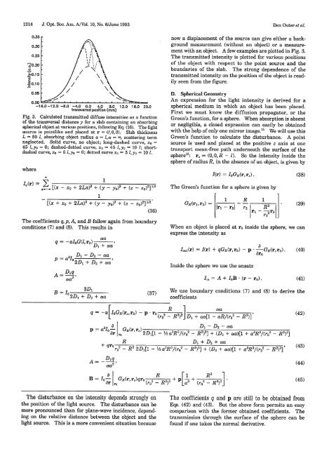
1214 J. Opt. Soc. Am. A/Vol. 10, No. 6/June 1993 0.35 0.30 0.25 ,0.20 / .10.10/ Z005 . /X ll 0.05 0.00 - -1 6.0 -12.0 -8.0 -4.0 0.0 4.0 8.0 12.0 1 6.0 20.0 transversal position (mm) Fig. 3. Calculated transmitted diffuse intensities as a function of the transversal distance y for a slab containing an absorbing spherical object at various positions, following Eq. (16). The light source is pointlike and placed at r= (1,0,0). Slab thickness L = 50 1, absorbing object radius a = , = , scattering term neglected. Solid curve, no object; long-dashed curve, x = 45 ,yo = 0; dashed-dotted curve, x = 45 ,yo = 10 1; shortdashed curve, xo = 5 1, yo = 0; dotted curve x 0 = 5 1, yo = 10 1. where nIr [(x - xo + 2Ln) 2 + (y - yo) 2 + (z - Z2]12 1 [(x + x 0 + 2Ln) 2 + (y - yo) 2 + (Z - ZO)2]112 (36) The coefficients q, p, A, and B follow again from boundary conditions (7) and (8). This results in q = -aIOG(, rO) aa' D + aa = D - D2- a a 3 IO 2 D + D 2 + a A =Dq aa2 B = + 3D+ D1 2,+ D2 + aa~ q = -a[IoGR(rsrO) - p ro p = a 3 I 0a- GR(r, r)2 A = _ Dlq aa2 The disturbance on the intensity depends strongly on the position of the light source. The disturbance can be more pronounced than for plane-wave incidence, depending on the relative distance between the object and the light source. This is a more convenient situation because now a displacement of the source can give either a background measurement (without an object) or a measurement with an object. A few examples are plotted in Fig. 3. The transmitted intensity is plotted for various positions of the object with respect to the point source and the boundaries of the slab. The strong dependence of the transmitted intensity on the position of the object is readily seen from the figure. D. Spherical Geometry An expression for the light intensity is derived for a spherical medium in which an object has been placed. First we must know the diffusion propagator, or the Green's function, for a sphere. When absorption is absent or negligible, a closed expression can easily be obtained with the help of only one mirror image. 5 We will use this Green's function to calculate the disturbance. A point source is used and placed at the positive z axis at one transport mean-free path underneath the surface of the sphere' 6 : r, = (O,O,R - ). So the intensity inside the sphere of radius R, in the absence of an object, is given by I(r) = IGR(r,r). (38) The Green's function for a sphere is given by 1 GR (rl,r 2) = I 2 R 1 r2 R2 ri - _X`2 r22 (39) When an object is placed at r inside the sphere, we can express the intensity as Iout(r) = I(r) + qGR(r,ro) - P a GR(rro). aro Inside the sphere we use the ansatz (40) Iin = A + IoB (r - r). (41) We use boundary conditions (7) and (8) to derive the coefficients R 1 cia 2 (r0 - R2)2J Di + aa[l 2 - 2 aR/(rb - R )] D- -D2-aa al. ro 2D,[1 - /2 a3R3 2 /(r0 - 2 3 R ) ] + (D2 + aa)[1 + a 3 R3/(r 2 R -R2)3] +qor2- R 22DJ[1 - /2 a R 3 /(ro 2 a R [I R 3 ar ro (ro2 i) 3+( 0 2 -R23 D, + D 2 + aa - R 2 ) 3 ] + (D 2 + aa)[1 + a3R 3 /(ro 2 - R2)3] Den Outer et al. (42) (43) (44) (45) The coefficients q and p are still to be obtained from Eqs. (42) and (43). But the above form permits an easy comparison with the former obtained coefficients. The transmission through the surface of the sphere can be found if one takes the normal derivative.
Den Outer et al. OBJECT S Le D Fig. 4. Experimental setup: L, laser, Sp, spatial filter; S, screen; C, cell with the scattering medium and the object; Le, lens for imaging the diffuse intensity on D, the one-dimensional diode array. 1.050 1 .000 0.950 0.900 M O0.850 - 0.800 c C S0.750 . transversal position (mm) Fig. 5. Transmitted intensity profiles from a cell containing a diffusive scattering suspension, for various positions of the embedded absorbing wire 4 = 350 ,m: a, x0 = 1.00 mm; b, xO= 2.60 mm, and c, x0 = 4.10 mm. The experimental data are shown together with the best numerical fits for Eq. (25): a, x0 = 1.41 ± 0.05 mm, D,/oaa = 0.95 ± 0.03; b, x0 = 2.86 + 0.05 mm, Di/ara = 1.04 + 0.03; c, xo = 4.33 + 0.05 mm, D,/aa = 1.11 ± 0.03. In all cases a = 0.175, bm, p = 0, 1 = 20 ± 3 and cell thickness L = 10.0 mm. 3. MEASUREMENTS The experimental setup for a plane-wave transmission measurement is shown in Fig. 4. A 7-mW continuouswave He-Ne laser beam (A = 633 nm) is spatially filtered and expanded to a radius of approximately 20 cm to produce a flat beam profile. Part of this beam impinges upon the cell with the object in the highly scattering medium. The transmitted light, imaged on a one-dimensional diode array, is read out by a computer. The spatial resolution is approximately 60 jum. When backscattering experiments Vol. 10, No. 6/June 1993/J. Opt. Soc. Am. A 1215 are done, the illuminated side of the cell is imaged on the diode array. Care should be taken for the window ref lection of the cell. We have used two different cells. The first has a thickness of 4 mm and 4 mm X 40 mm X 40 mm sized windows, the second has a variable thickness of 5 or 10 mm and windows with size 20 mm X 60 mm X 60 mm. Complications are introduced by the glass windows, since light is totally reflected by the window-air interface when the angle between the surface normal and the light ray is beyond the critical angle. This reflected light either enters the sample again or is reflected by it. As a consequence, every point source at the boundary of the scattering medium is spread out in a triangular intensity profile, and a nonnegligible deformation of the intensity occurs. Transmission experiments on absorbing objects suffer most from this effect, because the intensity profile relative to the background is the largest. This deformation can be reproduced if one convolutes the calculated profiles with the triangular intensity profile. The latter should be calculated on the basis of multiple reflections inside the window. However, this will extend the fitting procedure by the introduction of more fit parameters, and therefore the procedure is not favorable. We have chosen to reduce the effect of these reflections on the intensity profile by using a cell with thick windows. The total internal reflected light is well separated from its source, and in most cases the light is reflected beside the sample. (An antireflection coating on the windows would not have solved this problem because the coating cannot reduce total internal reflections.) For plane-wave incident experiments we perform ratio measurements to correct for the sensitivity of the individual diodes and to correct for the remaining beam profile. Depending on the strength of the signal, integration times vary from 10 s to 3 min. The scattering medium consists of suspended TiO 2 rutile particles, having an average size of 220 nm, in glycerine. We calculate the transport meanfree path from the measured scattering mean-free path by means of Mie theory.' 0 In Fig. 5 we present transmission measurements for absorbing rods. We use a 0.35-mm pencil embedded in a scattering medium with a transport mean-free path of 20 tum. The thickness of the cell is 10.0 mm. The solid curves are the best numerical fits of Eq. (25) to the measured profiles. Here the position and the absorbing Table 1. Fits of the Calculated Line Shape to Experimental Data Obtained from a Transmission Experiment with an Absorbing Roda Experimental Fitted Absorption Experimental Fitted Position Normal Normal Strength Position Relative to Relative to Position (mm) Position (mm) D/aa First Position (mm) First Position (mm) 0.75 ± 0.05 1.23 ± 0.02 0.95 ± 0.03 0 0 1.40 ± 0.05 1.91 ± 0.02 0.99 ± 0.03 0.65 ± 0.07 0.68 ± 0.03 2.30 ± 0.05 2.78 ± 0.02 1.04 ± 0.03 1.55 ± 0.07 1.55 ± 0.03 3.50 ± 0.05 3.91 ± 0.02 1.10 ± 0.03 2.75 ± 0.07 2.68 ± 0.03 4.95 ± 0.05 5.28 ± 0.02 1.11 ± 0.03 4.20 ± 0.07 4.05 ± 0.03 6.30 ± 0.05 6.67 ± 0.02 0.96 ± 0.03 5.55 ± 0.07 5.44 ± 0.03 7.80 ± 0.05 8.2 ± 0.1 0.8 ± 0.1 7.05 ± 0.07 7.0 ± 0.1 9.30 ± 0.05 9.8 ± 0.1 0.6 ± 0.1 8.55 ± 0.07 8.6 ± 0.1 aIn all cases the scattering contribution is neglected, p = 0; the size of the rod 0 = 350 Am, and the diffusion constant inside the rod D 2
Page 1 and 2: Den Outer et al. Vol. 10, No. 6/Jun
Page 3 and 4: Den Outer et al. third is the dipol
Page 5: Den Outer et al.- 1 .00 0.95 0.90 '
Page 9 and 10: Den Outer et al. Table 3. Fits of t

Location of objects in multiple-scattering media - COPS

You also want an ePaper? Increase the reach of your titles

Delete template?

Save as template?