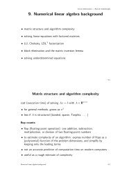
2. Quasi-Newton methods

• variable metric methods
• quasi-Newton methods
• BFGS update
2. Quasi-Newton methods
• limited-memory quasi-Newton methods
EE236C (Spring 2011-12)
2-1

Newton method for unconstrained minimization
minimize f(x)
f convex, twice continously differentiable
Newton method
x + = x−t∇ 2 f(x) −1 ∇f(x)
• advantages: fast convergence, affine invariance
• disadvantages: requires second derivatives, solution of linear equation
can be too expensive for large scale applications
Quasi-Newton methods 2-2

Variable metric methods
x + = x−tH −1 ∇f(x)
H ≻ 0 is approximation of the Hessian at x, chosen to:
• avoid calculation of second derivatives
• simplify computation of search direction
‘variable metric’ interpretation (EE236B, lecture 10, page 11)
∆x = −H −1 ∇f(x)
is steepest descent direction at x for quadratic norm
�z�H = � z T Hz �1/2
Quasi-Newton methods 2-3

Quasi-Newton methods
given starting point x (0) ∈ domf, H0 ≻ 0
for k = 1,2,..., until a stopping criterion is satisfied
1. compute quasi-Newton direction ∆x = −H −1
k−1 ∇f(x(k−1) )
2. determine step size t (e.g., by backtracking line search)
3. compute x (k) = x (k−1) +t∆x
4. compute Hk
• different methods use different rules for updating H in step 4
• can also propagate H −1
k to simplify calculation of ∆x
Quasi-Newton methods 2-4

Broyden-Fletcher-Goldfarb-Shanno (BFGS) update
BFGS update
where
inverse update
Hk = Hk−1+ yyT
yTs − Hk−1ssTHk−1 sTHk−1s s = x (k) −x (k−1) , y = ∇f(x (k) )−∇f(x (k−1) )
H −1
k =
�
I − syT
yT �
H
s
−1
�
k−1 I − ysT
yT �
s
+ ssT
y T s
• note that y T s > 0 for strictly convex f; see page 1-11
• cost of update or inverse update is O(n 2 ) operations
Quasi-Newton methods 2-5

Positive definiteness
if y T s > 0, BFGS update preserves positive definitess of Hk
proof: from inverse update formula,
v T H −1
k v =
�
v − sTv sTy y
�T
H −1
�
k−1 v − sTv sTy y
�
• if Hk−1 ≻ 0, both terms are nonnegative for all v
+ (sT v) 2
y T s
• second term is zero only if s T v = 0; then first term is zero only if v = 0
this ensures that ∆x = −H −1
k ∇f(x(k) ) is a descent direction
Quasi-Newton methods 2-6

Secant condition
BFGS update satisfies the secant condition Hks = y, i.e.,
Hk(x (k) −x (k−1) ) = ∇f(x (k) )−∇f(x (k−1) )
interpretation: define second-order approximation at x (k)
fquad(z) = f(x (k) )+∇f(x (k) ) T (z −x (k) )+ 1
2 (z −x(k) ) T Hk(z −x (k) )
secant condition implies that gradient of fquad agrees with f at x (k−1) :
∇fquad(x (k−1) ) = ∇f(x (k) )+Hk(x (k−1) −x (k) )
= ∇f(x (k−1) )
Quasi-Newton methods 2-7

secant method
for f : R → R, BFGS with unit step size gives the secant method
x (k+1) = x (k) − f′ (x (k) )
f ′
quad (z)
f ′ (z)
Hk
x (k−1)
, Hk = f′ (x (k) )−f ′ (x (k−1) )
x (k) −x (k−1)
x (k) x (k+1)
Quasi-Newton methods 2-8

global result
Convergence
if f is strongly convex, BFGS with backtracking line search (EE236B,
lecture 10-6) converges from any x (0) , H (0) ≻ 0
local convergence
if f is strongly convex and ∇ 2 f(x) is Lipschitz continuous, local
convergence is superlinear: for sufficiently large k,
�x (k+1) −x ⋆ �2 ≤ ck�x (k) −x ⋆ �2 → 0
where ck → 0 (cf., quadratic local convergence of Newton method)
Quasi-Newton methods 2-9

f(x (k) ) − f ⋆
n = 100, m = 500
10 2
10 0
10 -2
10 -4
10 -6
10 -8
10 -10
Newton
minimize c T x−
10 0 1 2 3 4 5 6 7 8 9
-12
k
Example
m�
i=1
log(bi−a T i x)
10 -10
cost per Newton iteration: O(n 3 ) plus computing ∇ 2 f(x)
cost per BFGS iteration: O(n 2 )
f(x (k) ) − f ⋆
10 2
10 0
10 -2
10 -4
10 -6
10 -8
BFGS
10 0 20 40 60 80 100 120 140
-12
Quasi-Newton methods 2-10
k

Square root BFGS update
to improve numerical stability, can propagate Hk in factored form
if Hk−1 = Lk−1L T k−1 then Hk = LkL T k with
where
Lk = Lk−1
�
I +
(α˜y − ˜s)˜sT
˜s T ˜s
˜y = L −1
k−1 y, ˜s = Lk−1s, α =
�
,
� T ˜s ˜s
yT �1/2
s
if Lk−1 is triangular, cost of reducing Lk to triangular is O(n 2 )
Quasi-Newton methods 2-11

Optimality of BFGS update
X = Hk solves the convex optimization problem
minimize tr(H −1
k−1 X)−logdet(H−1
k−1 X)−n
subject to Xs = y
• cost function is nonnegative, equal to zero only if X = Hk−1
• also known as relative entropy between densities N(0,X), N(0,Hk−1)
optimality result follows from KKT conditions: X = Hk satisfies
with
X −1 = H −1
k−1
ν = 1
s T y
− 1
2 (sνT +νs T ), Xs = y, X ≻ 0
�
2H −1
k−1y −
�
1+ yT H −1
k−1 y
y T s
Quasi-Newton methods 2-12
�
s
�

Davidon-Fletcher-Powell (DFP) update
switch Hk−1 and X in objective on previous page
minimize tr(Hk−1X −1 )−logdet(Hk−1X −1 )−n
subject to Xs = y
• minimize relative entropy between N(0,Hk−1) and N(0,X)
• problem is convex in X −1 (with constraint written as s = X −1 y)
• solution is ‘dual’ of BFGS formula
Hk =
(known as DFP update)
�
I − ysT
sT � �
Hk−1 I −
y
syT
sT �
y
pre-dates BFGS update, but is less often used
+ yyT
s T y
Quasi-Newton methods 2-13

Limited memory quasi-Newton methods
main disadvantage of quasi-Newton method is need to store Hk or H −1
k
limited-memory BFGS (L-BFGS): do not store H −1
k explicitly
• instead we store the m (e.g., m = 30) most recent values of
sj = x (j) −x (j−1) , yj = ∇f(x (j) )−∇f(x (j−1) )
• we evaluate ∆x = H −1
k ∇f(x(k) ) recursively, using
H −1
j =
�
I − sjy T j
y T j sj
�
H −1
j−1
�
I − yjs T j
y T j sj
�
+ sjs T j
y T j sj
for j = k,k −1,...,k −m+1, assuming, for example, H −1
k−m
• cost per iteration is O(nm); storage is O(nm)
Quasi-Newton methods 2-14
= I

References
• J. Nocedal and S. J. Wright, Numerical Optimization (2006), chapters
6 and 7
• J. E. Dennis and R. B. Schnabel, Numerical Methods for Unconstrained
Optimization and Nonlinear Equations (1983)
Quasi-Newton methods 2-15