lecture-19 journal bearings - NPTel - Indian Institute of Technology ...

Machine Design II Prof. K.Gopinath & Prof. M.M.Mayuram 

Indian Institute of Technology Madras 

Module 5 – SLIDING CONTACT BEARINGS 

Lecture 2 – HYDRODYNAMIC LUBRICATION OF JOURNAL BEARINGS 

THEORY AND PRACTICE 

Contents 

2.1 Petroff’s equation for bearing friction 

2.2 Analysis Problem 1 

2.3 Hydrodynamic lubrication of Journal bearings - theory 

2.4 Design charts for Hydrodynamic lubricated journal bearings 

2.5 Analysis Problem 2 

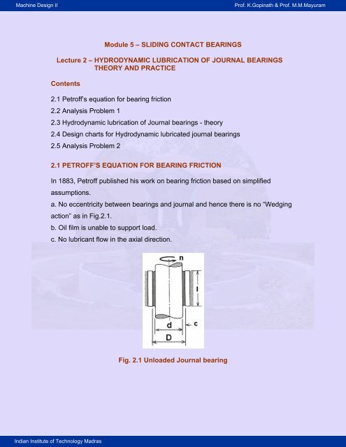
2.1 PETROFF’S EQUATION FOR BEARING FRICTION 

In 1883, Petroff published his work on bearing friction based on simplified 

assumptions. 

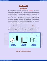
a. No eccentricity between bearings and journal and hence there is no “Wedging 

action” as in Fig.2.1. 

b. Oil film is unable to support load. 

c. No lubricant flow in the axial direction. 

Fig. 2.1 Unloaded Journal bearing


With reference to Fig.2.1, an expression for viscous friction drag torque is derived 

by considering the entire cylindrical oil film as the “liquid block” acted upon by 

force F. 

From Newton’s law of Viscosity: 


AU 

F=μ h 

(2.1) 

Fig. 2.2 Laminar flow of fluid in clearance space 

Where F = friction torque/shaft radius = 2 T f / d 

A= π d l 

U = π d n (Where n is in rps d is in m) 

h = c (Where c = radial clearance = 0.5(D-d)) 

r = d /2 

Substituting and solving for friction torque: 

2 3 

4 π μnlr 

T f � 

( 2.2) 

c


If a small radial load W is applied to the shaft, Then the frictional drag force f w 

and the friction 

Torque will be: 


Tf = f w = 0.5 f (d l p) d (2. 3) 

Equating eon. (2.2) and (2.3) and simplifying, we get 

2 �μn��r � 

f�2π � �� 

(2.4) 

� p ��c� 

Where r = 0.5 d and u is Pa. 

This is known as Petroff’s equation for bearing friction. It gives reasonable 

estimate of co-efficient of friction of lightly loaded bearings. 

The first quantity in the bracket stands for bearing modulus and second one 

stands for clearance ratio. Both are dimensionless parameters of the bearing. 

Clearance ratio normally ranges from 500 to 1000 in bearings. 

2.2 PETROFF’S EQUATION FOR BEARING FRICTION – Problem 1 

A machine journal bearing has a journal diameter of 150 mm and length of 120 

mm. The bearing diameter is 150.24 mm. It is operating with SAE 40 oil at 65 o C. 

The shaft is carrying a load of 8 kN and rotates at 960 rpm. Estimate the bearing 

coefficient of friction and power loss using Petroff’s equation. 

Data: d = 0.15m; D =0.15024m; l = 0.12 m; F=8kN; 

SAE 40 oil To = 65 o C; n = 960/60 = 16 rps. 

Q 1, f =? , Nloss =? 

Solution: 

r = 0.5d = 0.5 x 0.15 = 0.075 m 

c = (D-d) /2 = 0.00012 m 

p = F/dl = 8000/ 150x 120 = 0.44 MPa= 44X10 4 Pa


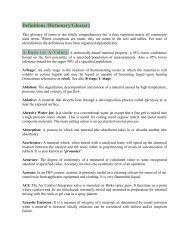
Viscosity of SAE 40 at 65 o C, μ = 30 mPa.s = 30x10 -3 Ns/m 2 

(a) 


2 2� 

�3 

� 

4 

�μn��r� 30 x10 x16 � 0.075 � 

f� 2π� �� 2π � �� 

��0.0134 

� p ��c� � 44x10 ��0.00012 

� 

Fig.2.3a Viscosity – temperature curves of SAE graded oils 

(b) Friction Torque Tf = f F r = 0.0134 x 8000 x 0.075 = 8.067 Nm 

ω = 2πn /60 = 2 x 3.14 x 960 / 60 = 100.48 rad/s 

Power loss: Nloss = Tf ω = 8.067 x 100.48 = 811 W


2.3 HYDRODYNAMIC LUBRICATION THEORY 

Beauchamp Tower’s exposition of hydrodynamic behavior of journal bearings in 

1880s and his observations drew the attention of Osborne Reynolds to carryout 

theoretical analysis. This has resulted in a fundamental equation for 

hydrodynamic lubrication. This has provided a strong foundation and basis for 

the design of hydro-dynamic lubricated bearings. 

In his theoretical analysis, Reynolds made the following assumptions: 

a) The fluid is Newtonian. 

b) The fluid is incompressible. 

c) The viscosity is constant throughout the film. 

d) The pressure does not vary in the axial direction. 

e) The bearing and journal extend infinitely in the z direction. i.e., no lubricant 

flow in the z direction. 

f) The film pressure is constant in the y direction. Thus the pressure depends 

on the x coordinate only. 

g) The velocity of particle of lubricant in the film depends only on the coordinates 

x and y. 

h) The effect of inertial and gravitational force is neglected. 

i) The fluid experience laminar flow. 

2.3.1 Reynolds’ Equation 

As shown in Fig.2.4, the Forces acting on a fluid element of height dy, width dx, 

velocity u, and top to bottom velocity gradient du is considered. 

For the equilibrium of forces in the x direction acting on the fluid element acting 

on the fluid element shown in Fig. 2.5 

dp 

�� 

-pdydz ��dxdz �(p � dx)dydz - ( �� dy)dxdz �0 

2.5 

dx �y 


� �


which reduces to 


Fig.2.4 Pressure and viscous forces acting on an 

element of lubricant. Only X components are shown 

dp �� 

� 

dx �y 

The equation for absolute viscosity is given as 

(2.6) 

µ = F h /(A U) (2.7) 

In eqn. (7) is the shear stress. 

�u 

�� 

�y 

In eqn. (2.7) is the shear stress. 

F 

�� 

A 

(2.8) 

where the partial derivatives is used since the velocity u depends upon both x 

and y. Substituting eqn (8) in (6), we get 

2 

dp � u 

�� (2.9) 

2 

dx �y



Fig.2.5 Pressure and viscous forces acting on an 

element of lubricant. Only X components are shown 

Rearranging the terms, we get 

2 

� u 1dp 

� 2 

�y 

� dx 

(2.10) 

Holding x constant and integrating twice with respect to y gives 

�u 1�dp � 

� � y�C 1 

� � 

� (2.11) 

y �dx � 

� 2 

1 dp y 

� 

u� � �C1y�C 2� 

( 2.12) 

� �dx 2 

�


The assumption of no slip between the lubricants and the boundary surfaces 

gives boundary conditions enabling C1 and C2 to be evaluated: 

u=0 at y=0, u=U at y=h 

Hence, 


U�hdp 2 U 

C1 � � �y�hy�� y (2.13) 

h 2dx h 

and C 2=0 

(2.14) 

Substituting the values of C1 and C2 in Equation (2.12) 

we get, 

1 dp 2 U 

u � �y�hy�� y (2.15) 

2�dx h 

Fig. 2.6 Velocity distribution in the oil film 

Velocity Distribution of the Lubricant Film shown in Fig.2.6 consists of two terms 

on the right hand side.



1 dp 2 U 

u � �y �hy�� 

y 

2�dx h 

Parabolic Linear – Dashed 

Fig. 2.7 Velocity gradient in the oil film 

At the section when pressure is a maximum and the velocity gradient is linear. 

dp 0 

dy � 

Let the volume of lubricant per-unit time flowing across the section containing the 

element in Fig. 2.6 be Qf. For unit width in the Z direction, 

�� 

� 

h 3 

Uh h dp 

Qfudy (2.16) 

2 12 dx 

o 

For an in-compressible liquid, the flow rate must be the same for all cross 

sections, which means that 

dQf � 0 (2.17) 

dx 

Differentiating equation (2.16) with respect to x and equating to zero,


Or 


� 3 

dQ � 

f Udh d h dp 

� � � ��0 

(2.18) 

dx 2 dx dx �12�dx� � 3 

d h dp � dh 

� � � 6 U 

(2.19) 

dx � � dx � dx 

This is the classical Reynolds’ equation for one dimensional flow. This is valid for 

long bearings. 

In short bearings, flow in the Z direction or end leakage has to be taken into 

account. A similar development gives the Reynolds’ Equation for two dimensional 

flows: 

3 3 

d �hdp � d �hdp � dh 

� � � � � � 6 U (2.20) 

dx � � dx � dz � � dz � dx 

Modern bearings are short and (l / d) ratio is in the range 0.25 to 0.75. This 

causes flow in the z direction (the end leakage) to a large extent of the total flow. 

For short bearings, Ockvirk has neglected the x terms and simplified the 

Reynolds’ equation as: 

d �� 3 

d h dp �� 

dh 

�� 

�� 

6 U 

(2.21) ( 2.21) 

dz �� 

dz �� 

dx 

Unlike previous equations (2.19) and (2. 20), equation (2. 21) can be readily 

integrated and used for design and analysis purpose. The procedure is known as 

Ocvirk’s short bearing approximation. 

2.4 DESIGN CHARTS FOR HYDRODYNAMIC BEARINGS 

Solutions to eqn.2.19 were developed in first decade of 20th century and were 

applicable for long bearings and give reasonably good results for bearings with


(l / d) ratios more than 1.5. Ocvirk’s short bearing approximation on the other 

hand gives accurate results for bearings with (l /d) ratio up to 0.25 and often 

provides reasonable results for bearings with (l / d) ratios between 0.25 and 0.75. 

Raimondi and Boyd have obtained computerized solutions for Reynolds 

eqn. (2.20) and reduced them to chart form which provide accurate solutions for 

bearings of all proportions. Selected charts are shown in Figs. 2.8 to 2.15. 

All these charts are plots of non-dimensional bearing parameters as functions of 

the bearing characteristic number, or the Sommerfeld variable S which itself is a 

dimensionless parameter. 

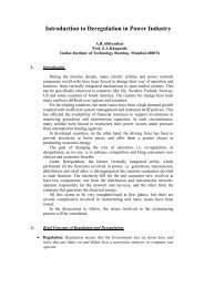
Fig.2.8 Chart for minimum film thickness variable and eccentricity ratio. 

The left shaded zone defines the optimum ho for minimum friction; the right 

boundary is the optimum ho for maximum load 

Indian Institute of Technology Madras


Fig.2.9 Chart for determining the position of the minimum film thickness ho 

for location refer Fig.2.10 


Fig.2.10 Stable hydrodynamic lubrication



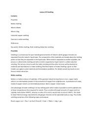
Fig. 2.11 Chart for coefficient of friction variable.



Fig. 2.12 Chart for flow variable.



Fig.2.13 Chart for determining the ratio of side flow to total flow. 

Fig. 2.14 Chart for determining the maximum film pressure.


Fig. 2.15 Chart for finding the terminating position of oil film and position of 

maximum film pressure 

2.5 DESIGN CHARTS FOR HYDRODYNAMIC BEARINGS – Problem 2 

A journal of a stationary oil engine is 80 mm in diameter. and 40 mm long. The 

radial clearance is 0.060mm. It supports a load of 9 kN when the shaft is rotating 

at 3600 rpm. The bearing is lubricated with SAE 40oil supplied at atmospheric 

pressure and average operating temperature is about 65 o C. Using Raimondi- 

Boyd charts analyze the bearing assuming that it is working under steady state 

condition. 

Data: d = 80 mm; l =40 mm; c = 0.06 mm; F = 9kN; 

n = 3600rpm = 60 rps; SAE 40 oil; To = 65 O C; 

Analysis: 

1. p= F / ld = 9 x1000 /40 x 80 = 2.813 MPa 

2. μ = 30 cP at 65 o C for SAE 40 oil from Fig. 2.3a. 

Indian Institute of Technology Madras


3. 


2 2 �3 

�r� ��n� � 40 � �30x10 x 60 � 

� � � � � 6 � 

S � 0.284 

c 

� 

p 

�� 

� 

� � � � �0.06 � � 2.813 x 10 � 

4. For S = 0.284 and l/d = ½, ho /c = 0.38 and 

ε = e /c = 0.62 from Fig.6. 

ho = 0.38xc = 0.382x 0.06=0.023mm = 23µm 

e = 0.62 x c = 0.62 x 0.06 = 0.037 mm 

Fig.2.3a Viscosity – temperature curves of SAE graded oils 

5. (r /c) f = 7.5, for S = 0.284 for l /d = ½ from Fig.2.11a. 

f = 7.5 x (c / r) = 7.5x (0.06/40) = 0.0113


Fig.2.8a Chart for minimum film thickness variable and eccentricity ratio. 

The left shaded zone defines the optimum ho for minimum friction; the right 

boundary is the optimum ho for maximum load 


Fig. 2.11a Chart for coefficient of friction variable


Fig.2.9a Chart for determining the position of minimum film thickness ho 

6. Φ = 46 o , for S = 0.284 for l /d = ½ from Fig.2.9a. 

7. (Q / r c n l) = 4.9, for S = 0.284 for l /d = ½ from Fig.2.12a. 

Q = 4.9 r c n l = 4.9 x 0.04 x 0.00006 x 60 x 0.04 

= 2.82x10 -5 m 3 /s = 28.2 cm 3 /s 

8. (Qs /Q) = 0.75, for S = 0.284 for l /d = ½ from Fig.2.13a. 


Qs = 0.75 Q = 0.75 x 28.2 = 21.2 cm 3 /s 

9. (p / p max) = 0.36, for S = 0.284 for l /d = ½ from Fig.2.14a. 

puma = p /0.36 = 2.813 / 0.36 = 7.8 MPa 

10. θpox = 61.5 o and θpuma = 17.5 o , for S = 0.284 for l /d = ½ from Fig.2.15a.



Fig. 2.12a Chart for flow variable



Fig.2.13a Chart for determining the ratio of side flow to total flow 

Fig. 2.14a Chart for determining the maximum film pressure


Fig. 2.15a Chart for finding the terminating position of oil film and position 

of maximum film pressure 


Fig.2.10a Stable hydrodynamic lubrication 

---------------------------

lecture-19 journal bearings - NPTel - Indian Institute of Technology ...

You also want an ePaper? Increase the reach of your titles

Delete template?

Save as template?