Chapter 4 Finite Element Methods - Humboldt-Universität zu Berlin
Chapter 4 Finite Element Methods - Humboldt-Universität zu Berlin
Chapter 4 Finite Element Methods - Humboldt-Universität zu Berlin

You also want an ePaper? Increase the reach of your titles
YUMPU automatically turns print PDFs into web optimized ePapers that Google loves.
<strong>Chapter</strong> 4<br />
<strong>Finite</strong> <strong>Element</strong> <strong>Methods</strong><br />
Susanne C. Brenner 1 and Carsten Carstensen 2<br />
1 University of South Carolina, Columbia, SC, USA<br />
2 <strong>Humboldt</strong>-<strong>Universität</strong> <strong>zu</strong> <strong>Berlin</strong>, <strong>Berlin</strong>, Germany<br />
1 Introduction 73<br />
2 Ritz–Galerkin <strong>Methods</strong> for Linear Elliptic<br />
Boundary Value Problems 74<br />
3 <strong>Finite</strong> <strong>Element</strong> Spaces 77<br />
4 A Priori Error Estimates for <strong>Finite</strong> <strong>Element</strong><br />
<strong>Methods</strong> 82<br />
5 A Posteriori Error Estimates and Analysis 85<br />
6 Local Mesh Refinement 98<br />
7 Other Aspects 104<br />
Acknowledgments 114<br />
References 114<br />
1 INTRODUCTION<br />
The finite element method is one of the most widely<br />
used techniques in computational mechanics. The mathematical<br />
origin of the method can be traced to a paper<br />
by Courant (1943). We refer the readers to the articles<br />
by Babuˇska (1994) and Oden (1991) for the history<br />
of the finite element method. In this chapter, we<br />
give a concise account of the h-version of the finite<br />
element method for elliptic boundary value problems in<br />
the displacement formulation, and refer the readers to<br />
the theory of <strong>Chapter</strong> 5 and <strong>Chapter</strong> 9 of this Volume.<br />
This chapter is organized as follows. The finite element<br />
method for elliptic boundary value problems is based on the<br />
Encyclopedia of Computational Mechanics, Edited by Erwin<br />
Stein, René de Borst and Thomas J.R. Hughes. Volume 1: Fundamentals.<br />
© 2004 John Wiley & Sons, Ltd. ISBN: 0-470-84699-2.<br />
Ritz–Galerkin approach, which is discussed in Section 2.<br />
The construction of finite element spaces and the a priori<br />
error estimates for finite element methods are presented<br />
in Sections 3 and 4. The a posteriori error estimates for<br />
finite element methods and their applications to adaptive<br />
local mesh refinements are discussed in Sections 5 and 6.<br />
For the ease of presentation, the contents of Sections 3<br />
and 4 are restricted to symmetric problems on polyhedral<br />
domains using conforming finite elements. The extension<br />
of these results to more general situations is outlined in<br />
Section 7.<br />
For the classical material in Sections 3, 4, and 7, we are<br />
content with highlighting the important results and pointing<br />
to the key literature. We also concentrate on basic<br />
theoretical results and refer the readers to other chapters<br />
in this encyclopedia for complications that may arise<br />
in applications. For the recent development of a posteriori<br />
error estimates and adaptive local mesh refinements<br />
in Sections 5 and 6, we try to provide a more comprehensive<br />
treatment. Owing to space limitations many significant<br />
topics and references are inevitably absent. For<br />
in-depth discussions of many of the topics covered in<br />
this chapter (and the ones that we do not touch upon),<br />
we refer the readers to the following survey articles<br />
and books (which are listed in alphabetical order) and<br />
the references therein (Ainsworth and Oden, 2000; Apel,<br />
1999; Aziz, 1972; Babuˇska and Aziz, 1972; Babuˇska and<br />
Strouboulis, 2001; Bangerth and Rannacher, 2003; Bathe,<br />
1996; Becker, Carey and Oden, 1981; Becker and Rannacher,<br />
2001; Braess, 2001; Brenner and Scott, 2002;<br />
Ciarlet, 1978, 1991; Eriksson et al., 1995; Hughes, 2000;<br />
Oden and Reddy, 1976; Schatz, Thomée and Wendland,<br />
1990; Strang and Fix, 1973; Szabó and Babuˇska, 1991;<br />
Verfürth, 1996; Wahlbin, 1991, 1995; Zienkiewicz and Taylor,<br />
2000).
74 <strong>Finite</strong> <strong>Element</strong> <strong>Methods</strong><br />
2 RITZ–GALERKIN METHODS FOR<br />
LINEAR ELLIPTIC BOUNDARY<br />
VALUE PROBLEMS<br />
In this section, we set up the basic mathematical framework<br />
for the analysis of Ritz–Galerkin methods for linear<br />
elliptic boundary value problems. We will concentrate on<br />
symmetric problems. Nonsymmetric elliptic boundary value<br />
problems will be discussed in Section 7.1.<br />
2.1 Weak problems<br />
Let � be a bounded connected open subset of the Euclidean<br />
space Rd with a piecewise smooth boundary. For a positive<br />
integer k, the Sobolev space H k (�) is the space of square<br />
integrable functions whose weak derivatives up to order k<br />
are also square integrable, with the norm<br />
⎛<br />
�v�H k (�) = ⎝ �<br />
�<br />
�<br />
�<br />
∂<br />
�<br />
αv ∂xα ⎞<br />
� 1/2<br />
�2<br />
� ⎠<br />
�<br />
The seminorm<br />
|α|≤k<br />
L2(�)<br />
� �<br />
|α|=k �(∂αv/∂xα )�2 �1/2 L2(�) will be deno-<br />
ted by |v| H k (�) . We refer the readers to Nečas (1967),<br />
Adams (1995), Triebel (1978), Grisvard (1985), and Wloka<br />
(1987) for the properties of the Sobolev spaces. Here we<br />
just point out that �·� H k (�) is a norm induced by an inner<br />
product and H k (�) is complete under this norm, that is,<br />
H k (�) is a Hilbert space. (We assume that the readers are<br />
familiar with normed and Hilbert spaces.)<br />
Using the Sobolev spaces we can represent a large class<br />
of symmetric elliptic boundary value problems of order 2m<br />
in the following abstract weak form:<br />
Find u ∈ V , a closed subspace of a Sobolev space H m (�),<br />
such that<br />
a(u,v) = F(v) ∀ v ∈ V (1)<br />
where F : V → R is a bounded linear functional on V and<br />
a(·, ·) is a symmetric bilinear form that is bounded and<br />
V -elliptic, that is,<br />
�<br />
�a(v 1 ,v 2 ) � � ≤ C 1 �v 1 � H m (�) �v 2 � H m (�) ∀ v 1 ,v 2 ∈ V (2)<br />
a(v, v) ≥ C 2 �v� 2 H m (�) ∀ v ∈ V (3)<br />
Remark 1. We use C, with or without subscript, to<br />
represent a generic positive constant that can take different<br />
values at different occurrences.<br />
Remark 2. Equation (1) is the Euler–Lagrange equation<br />
for the variational problem of finding the minimum<br />
of the functional v ↦→ 1<br />
2a(v, v) − F(v) on the space V .In<br />
mechanics, this functional often represents an energy and its<br />
minimization follows from the Dirichlet principle. Furthermore,<br />
the corresponding Euler–Lagrange equations (also<br />
called first variation) (1) often represent the principle of<br />
virtual work.<br />
It follows from conditions (2) and (3) that a(·, ·) defines<br />
an inner product on V which is equivalent to the inner<br />
product of the Sobolev space H m (�). Therefore the existence<br />
and uniqueness of the solution of (1) follow immediately<br />
from (2), (3), and the Riesz Representation Theorem<br />
(Yosida, 1995; Reddy, 1986; Oden and Demkowicz, 1996).<br />
The following are typical examples from computational<br />
mechanics.<br />
Example 1. Let a(·, ·) be defined by<br />
�<br />
a(v1 ,v2 ) = ∇v1 ·∇v2 dx (4)<br />
For f ∈ L 2 (�), the weak form of the Poisson problem<br />
�<br />
−�u = f on �, u = 0 on Ɣ,<br />
∂u<br />
= 0 on ∂� \ Ɣ<br />
∂n<br />
(5)<br />
where Ɣ is a subset of ∂� with a positive (d − 1)dimensional<br />
measure, is given by (1) with V ={v ∈<br />
H 1 (�): v � � = 0} and<br />
Ɣ<br />
�<br />
F(v) = fvdx = (f, v) L2(�) (6)<br />
�<br />
For the pure Neumann problem where Ɣ =∅, since<br />
the gradient vector vanishes for constant functions, an<br />
appropriate function space for the weak problem is V =<br />
{v ∈ H 1 (�): (v, 1) L2(�) = 0}.<br />
The boundedness of F and a(·, ·) is obvious and the<br />
coercivity of a(·, ·) follows from the Poincaré–Friedrichs<br />
inequalities (Nečas, 1967):<br />
� ��<br />
��<br />
� �<br />
�v�L2(�) ≤ C |v| H 1 (�) + �<br />
� v ds�<br />
� ∀ v ∈ H<br />
Ɣ<br />
1 (�) (7)<br />
� ��<br />
��<br />
� �<br />
�v�L2(�) ≤ C |v| H 1 (�) + �<br />
� v dx�<br />
� ∀ v ∈ H 1 (�) (8)<br />
�<br />
Example 2. Let � ⊂ Rd (d = 2, 3) and v ∈ [H 1 (�)] d be<br />
the displacement of an elastic body. The strain tensor ɛ(v)<br />
is given by the d × d matrix with components<br />
� �<br />
∂vi<br />
ɛ ij (v) = 1<br />
2<br />
∂x j<br />
+ ∂v j<br />
∂x i<br />
(9)
and the stress tensor σ(v) is the d × d matrix defined by<br />
σ(v) = 2µɛ(v) + λ (div v) δ (10)<br />
where δ is the d × d identity matrix and µ > 0andλ > 0<br />
are the Lamé constants.<br />
Let the bilinear form a(·, ·) be defined by<br />
� d�<br />
�<br />
a(v1 , v2 ) = σij (v1 ) ɛij (v2 ) dx = σ(v1 ): ɛ(v2 ) dx<br />
�<br />
i,j=1<br />
(11)<br />
For f ∈ [L 2 (�)] d , the weak form of the linear elasticity<br />
problem (Ciarlet, 1988)<br />
div [σ(u)] = f on �, u = 0 on Ɣ<br />
[σ(u)]n = 0 on ∂� \ Ɣ (12)<br />
where Ɣ is a subset of ∂� with a positive (d − 1)dimensional<br />
measure, is given by (1) with V ={v ∈<br />
[H 1 (�)] d : v � � Ɣ = 0} and<br />
�<br />
F(v) =<br />
�<br />
�<br />
f · v dx = ( f , v) L2(�)<br />
(13)<br />
For the pure traction problem where Ɣ =∅,thestrain<br />
tensor vanishes for all infinitesimal rigid motions, i.e., displacement<br />
fields of the form m = a + ρ x, wherea∈Rd ,<br />
ρ is a d × d antisymmetric matrix and x = (x1 ,...,xd ) t<br />
is the position vector. In this case an appropriate function<br />
space for the weak problem is V ={v ∈ [H 1 (�)] d : �<br />
� ∇×<br />
v dx = 0 = �<br />
� v dx}.<br />
The boundedness of F and a(·, ·) is obvious and the coercivity<br />
of a(·, ·) follows from Korn’s inequalities (Friedrichs,<br />
1947; Duvaut and Lions, 1976; Nitsche, 1981) (see <strong>Chapter</strong>2,Volume2):<br />
�<br />
�v�H 1 (�) ≤ C �ε(v)�L2(�) +<br />
��<br />
��<br />
� �<br />
�<br />
� v ds�<br />
� ∀ v ∈ [H<br />
Ɣ<br />
1 (�)] d ,<br />
(14)<br />
�<br />
�v�H 1 (�) ≤ C �ε(v)�L2(�) +<br />
��<br />
�<br />
�<br />
�<br />
�<br />
� ∇×v ds�<br />
� +<br />
��<br />
��<br />
� �<br />
�<br />
� v dx�<br />
�<br />
�<br />
∀ v ∈ [H 1 (�)] d<br />
�<br />
(15)<br />
Example 3. Let � be a domain in R2 and the bilinear<br />
form a(·, ·) be defined by<br />
� �<br />
a(v1 ,v2 ) = �v1�v2 + (1 − σ)<br />
�<br />
�<br />
× 2 ∂2v1 ∂<br />
∂x1∂x2 2v2 ∂x1∂x2 − ∂2 v 1<br />
∂x 2 1<br />
∂ 2 v 2<br />
∂x 2 2<br />
where σ ∈ (0, 1/2) is the Poisson ratio.<br />
− ∂2 v 1<br />
∂x 2 2<br />
∂2 ��<br />
v2 dx<br />
∂x 2 1<br />
(16)<br />
<strong>Finite</strong> <strong>Element</strong> <strong>Methods</strong> 75<br />
For f ∈ L2 (�), the weak form of the clamped plate<br />
bending problem (Ciarlet, 1997)<br />
� 2 u = f on �, u = ∂u<br />
= 0 on ∂� (17)<br />
∂n<br />
is given by (1), where V ={v ∈ H 2 (�): v = ∂v/∂n = 0<br />
on ∂�}=H 2 0 (�) and F is defined by (6). For the simply<br />
supported plate bending problem, the function space V is<br />
{v ∈ H 2 (�): v = 0on∂�}=H 2 (�) ∩ H 1 0 (�).<br />
For these problems, the coercivity of a(·, ·) is a consequence<br />
of the following Poincaré–Friedrichs inequality<br />
(Nečas, 1967):<br />
�v�H 1 (�) ≤ C|v| H 2 (�) ∀ v ∈ H 2 (�) ∩ H 1 0 (�) (18)<br />
Remark 3. The weak formulation of boundary value<br />
problems for beams and shells can be found in <strong>Chapter</strong> 8,<br />
this Volume and <strong>Chapter</strong> 3, Volume 2.<br />
2.2 Ritz–Galerkin methods<br />
In the Ritz–Galerkin approach for (1), a discrete problem<br />
is formulated as follows.<br />
Find ũ ∈ �V such that<br />
a(ũ, ˜v) = F(˜v) ∀˜v ∈ �V (19)<br />
where �V , the space of trial/test functions, is a finitedimensional<br />
subspace of V .<br />
The orthogonality relation<br />
a(u −ũ, ˜v) = 0 ∀˜v ∈ �V (20)<br />
follows by subtracting (19) from (1), and hence<br />
�u −ũ� a = inf<br />
˜v∈V �u −˜v� a<br />
(21)<br />
where �·� a = (a(·, ·)) 1/2 . Furthermore, (2), (3), and (21)<br />
imply that<br />
�u −ũ� H m (�) ≤<br />
� �1/2 C1<br />
C 2<br />
inf �u −˜v�H m (�)<br />
˜v∈�V<br />
(22)<br />
that is, the error for the approximate solution ũ is quasioptimal<br />
in the norm of the Sobolev space underlying the<br />
weak problem.<br />
The abstract estimate (22), called Cea’s lemma, reduces<br />
the error estimate for the Ritz–Galerkin method to a problem<br />
in approximation theory, namely, to the determination<br />
of the magnitude of the error of the best approximation of
76 <strong>Finite</strong> <strong>Element</strong> <strong>Methods</strong><br />
u by a member of �V . The solution of this problem depends<br />
on the regularity (smoothness) of u and the nature of the<br />
space �V .<br />
One can also measure u −ũ in other norms. For exam-<br />
ple, an estimate of �u −ũ� L2(�)<br />
can be obtained by the<br />
Aubin–Nitsche duality technique as follows. Let w ∈ V be<br />
the solution of the weak problem<br />
�<br />
a(v,w) = (u −ũ)v dx ∀ v ∈ V (23)<br />
�<br />
Then we have, from (20), (23), and the Cauchy–Schwarz<br />
inequality,<br />
�u −ũ� 2 L2(�) = a(u −ũ, w) = a(u −ũ, w −˜v)<br />
≤ C2�u −ũ�Hm (�) �w −˜v�H m (�) ∀˜v ∈ �V<br />
which implies that<br />
�u −ũ�L2(�) ≤ C �<br />
�<br />
�w −˜v�H m (�)<br />
2 inf<br />
�u −ũ�Hm (�)<br />
˜v∈�V �u −ũ�L2(�) (24)<br />
In general, since w can be approximated by members of �V<br />
to high accuracy, the term inside the bracket on the righthand<br />
side of (24) is small, which shows that the L2 error<br />
is much smaller than the H m error.<br />
The estimates (22) and (24) provide the basic a priori<br />
error estimates for the Ritz–Galerkin method in an abstract<br />
setting.<br />
On the other hand, the error of the Ritz–Galerkin method<br />
can also be estimated in an a posteriori fashion. Let the<br />
computable linear functional (the residual of the approximate<br />
solution ũ) R: V → R be defined by<br />
R(v) = a(u −ũ, v) = F(v)− a(ũ, v) (25)<br />
The global a posteriori error estimate<br />
�u −ũ�Hm (�) ≤ 1<br />
sup<br />
C2 v∈V<br />
|R(v)|<br />
�v� H m (�)<br />
(26)<br />
then follows from (3) and (25).<br />
Let D be a subdomain of � and H m 0 (D) be the subspace<br />
of V whose members vanish identically outside D. It<br />
follows from (25) and the local version of (2) that we also<br />
have a local a posteriori error estimate:<br />
�u −ũ� H m (D) ≥ 1<br />
C 1<br />
sup<br />
v∈H m<br />
0 (D)<br />
|R(v)|<br />
�v� H m (D)<br />
(27)<br />
The equivalence of the error norm with the dual norm of<br />
the residual will be the point of departure in Section 5.1.2<br />
(cf. (70)).<br />
2.3 Elliptic regularity<br />
As mentioned above, the magnitude of the error of a<br />
Ritz–Galerkin method for an elliptic boundary value problem<br />
depends on the regularity of the solution. Here we give<br />
a brief description of elliptic regularity for the examples in<br />
Section 2.1.<br />
If the boundary ∂� is smooth and the homogeneous<br />
boundary conditions are also smooth (i.e. the Dirichlet and<br />
Neumann boundary condition in (5) and the displacement<br />
and traction boundary conditions in (12) are defined on<br />
disjoint components of ∂�), then the solution of the elliptic<br />
boundary value problems in Section 2.1 obey the classical<br />
Shift Theorem (Agmon, 1965; Nečas, 1967; Gilbarg and<br />
Trudinger, 1983; Wloka, 1987). In other words, if the righthand<br />
side of the equation belongs to the Sobolev space<br />
H ℓ (�), then the solution of a 2m-th order elliptic boundary<br />
problem belongs to the Sobolev space H 2m+ℓ (�).<br />
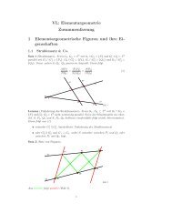
The Shift Theorem does not hold for domains with<br />
piecewise smooth boundary in general. For example, let<br />
� be the L-shaped domain depicted in Figure 1 and<br />
u(x) = φ(r) r 2/3 �<br />
2 �<br />
sin<br />
3<br />
θ − π<br />
2<br />
� �<br />
(28)<br />
where r = (x2 1 + x2 2 )1/2 and θ = arctan(x2 /x1 ) are the polar<br />
coordinates and φ is a smooth cut-off function that equals<br />
1for0≤r3/4.Itiseasytocheck<br />
that u ∈ H 1 0 (�) and −�u ∈ C∞ (�). LetDbe any open<br />
neighborhood of the origin in �. Then u ∈ H 2 (� \ D)<br />
but u �∈ H 2 (D). In fact u belongs to the Besov space<br />
B 5/3<br />
2,∞ (D) (Babuˇska and Osborn, 1991), which implies that<br />
u ∈ H 5/3−ɛ (D) for any ɛ > 0, but u �∈ H 5/3 (D) (see Triebel<br />
(1978) and Grisvard (1985) for a discussion of Besov<br />
spaces and fractional order Sobolev spaces). A similar situation<br />
occurs when the types of boundary condition change<br />
abruptly, such as the Poisson problem with mixed boundary<br />
conditions depicted on the circular domain in Figure 1,<br />
where the homogeneous Dirichlet boundary condition is<br />
assumed on the upper semicircle and the homogeneous<br />
Neumann boundary condition is assumed on the lower<br />
semicircle.<br />
Therefore (Dauge, 1988), for the second (respectively<br />
fourth) order model problems in Section 2.1, the solution<br />
in general only belongs to H 1+α (�) (respectively H 2+α (�))<br />
for some α ∈ (0, 1] even if the right-hand side of the<br />
equation belongs to C∞ (�).
(−1,1)<br />
(0,1)<br />
(0,0)<br />
−∆u = f<br />
(1,0)<br />
(−1,−1) u = 0 (1,−1)<br />
u = 0<br />
−∆u = f<br />
u/ n = 0<br />
Figure 1. Singular points of two-dimensional elliptic boundary<br />
value problems.<br />
For two-dimensional problems, the vertices of � and the<br />
points where the boundary condition changes type are the<br />
singular points (cf. Figure 1). Away from these singular<br />
points, the Shift Theorem is valid. The behavior of the<br />
solution near the singular points is also well understood.<br />
If the right-hand side function and its derivatives vanish<br />
to sufficiently high order at the singular points, then the<br />
Shift Theorem holds for certain weighted Sobolev spaces<br />
(Nazarov and Plamenevsky, 1994; Kozlov, Maz’ya and<br />
Rossman, 1997, 2001). Alternatively, one can represent the<br />
solution near a singular point as a sum of a regular part<br />
and a singular part (Grisvard, 1985; Dauge, 1988; Nicaise,<br />
1993). For a 2m-th order problem, the regular part of the<br />
solution belongs to the Sobolev space H 2m+k (�) if the<br />
right-hand side function belongs to H k (�), and the singular<br />
part of the solution is a linear combination of special<br />
functions with less regularity, analogous to the function<br />
in (28).<br />
The situation in three dimensions is more complicated<br />
due to the presence of edge singularities, vertex singularities,<br />
and edge-vertex singularities. The theory of threedimensional<br />
singularities remains an active area of research.<br />
3 FINITE ELEMENT SPACES<br />
<strong>Finite</strong> element methods are Ritz–Galerkin methods where<br />
the finite-dimensional trial/test function spaces are constructed<br />
by piecing together polynomial functions defined<br />
on (small) parts of the domain �. In this section, we<br />
describe the construction and properties of finite element<br />
spaces. We will concentrate on conforming finite elements<br />
here and leave the discussion of nonconforming finite elementstoSection7.2.<br />
3.1 The concept of a finite element<br />
A d-dimensional finite element (Ciarlet, 1978; Brenner<br />
and Scott, 2002) is a triple (K, P K , N K ),whereK is a<br />
closed bounded subset of R d with nonempty interior and<br />
<strong>Finite</strong> <strong>Element</strong> <strong>Methods</strong> 77<br />
a piecewise smooth boundary, PK is a finite-dimensional<br />
vector space of functions defined on K and NK is a basis of<br />
the dual space P ′ K . The function space PK is the space of<br />
the shape functions and the elements of NK are the nodal<br />
variables (degrees of freedom).<br />
The following are examples of two-dimensional finite<br />
elements.<br />
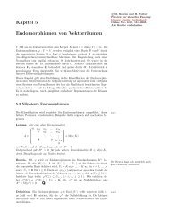
Example 4 (Triangular Lagrange <strong>Element</strong>s) Let K be a<br />
triangle, P K be the space P n of polynomials in two variables<br />
of degree ≤ n, and let the set N K consist of evaluations of<br />
shape functions at the nodes with barycentric coordinates<br />
λ 1 = i/n, λ 2 = j/n and λ 3 = k/n, wherei, j, k are nonnegative<br />
integers and i + j + k = n. Then (K, P K , N K )<br />
is the two-dimensional P n Lagrange finite element. The<br />
nodal variables for the P 1 , P 2 ,andP 3 Lagrange elements<br />
are depicted in Figure 2, where • (here and in the following<br />
examples) represents pointwise evaluation of shape<br />
functions.<br />
Example 5 (Triangular Hermite <strong>Element</strong>s) Let K be a<br />
triangle. The cubic Hermite element is the triple (K, P 3 ,<br />
N K ) where N K consists of evaluations of shape functions<br />
and their gradients at the vertices and evaluation of shape<br />
functions at the center of K. The nodal variables for the<br />
cubic Hermite element are depicted in the first figure in<br />
Figure 3, where Ž (here and in the following examples) represents<br />
pointwise evaluation of gradients of shape functions.<br />
By removing the nodal variable at the center (cf. the<br />
second figure in Figure 3) and reducing the space of shape<br />
functions to<br />
�<br />
v ∈ P 3 :6v(c) − 2<br />
+<br />
3�<br />
v(pi )<br />
i=1<br />
3�<br />
�<br />
(∇v)(pi ) · (pi − c) = 0 (⊃ P2 )<br />
i=1<br />
where p i (i = 1, 2, 3) and c are the vertices and center of<br />
K respectively, we obtain the Zienkiewicz element.<br />
The fifth degree Argyris element is the triple (K, P 5 , N K )<br />
where N K consists of evaluations of the shape functions and<br />
their derivatives up to order two at the vertices and evaluations<br />
of the normal derivatives at the midpoints of the edges.<br />
The nodal variables for the Argyris element are depicted<br />
in the third figure in Figure 3, where ○ and ↑ (here and<br />
Figure 2. Lagrange elements.
78 <strong>Finite</strong> <strong>Element</strong> <strong>Methods</strong><br />
Figure 3. Cubic Hermite element, Zienkiewicz element, fifth<br />
degree Argyris element and Bell element.<br />
in the following examples) represent pointwise evaluation<br />
of second order derivatives and the normal derivative of the<br />
shape functions, respectively.<br />
By removing the nodal variables at the midpoints of the<br />
edges (cf. the fourth figure in Figure 3) and reducing the<br />
space of shape functions to {v ∈ P 5 : (∂v/∂n) � � e ∈ P 3 (e) for<br />
each edge e}, we obtain the Bell element.<br />
Example 6 (Triangular Macro <strong>Element</strong>s) Let K be<br />
a triangle that is subdivided into three subtriangles by<br />
the center of K, P K be the space of piecewise cubic<br />
polynomials with respect to this subdivision that belong<br />
to C 1 (K), and let the set N K consist of evaluations of<br />
the shape functions and their first-order derivatives at the<br />
vertices of K and evaluations of the normal derivatives of<br />
the shape functions at the midpoints of the edges of K.Then<br />
(K, P K , N K ) is the Hsieh–Clough–Tocher macro element.<br />
The nodal variables for this element are depicted in the first<br />
figure in Figure 4.<br />
By removing the nodal variables at the midpoints of<br />
the edges (cf. the second figure in Figure 4) and reducing<br />
the space of shape functions to {v ∈ C 1 (K): v is piecewise<br />
cubic and (∂v/∂n) � � e ∈ P 1 (e) for each edge e}, we obtain<br />
the reduced Hsieh–Clough–Tocher macro element.<br />
Example 7 (Rectangular Tensor Product <strong>Element</strong>s)<br />
Let K be the rectangle [a1 ,b1 ] × [a2 ,b2 ], PK be the<br />
space spanned by the monomials xi 1xj 2 for 0 ≤ i, j ≤ n,<br />
and the set N K consist of evaluations of shape functions<br />
Figure 4. Hsieh–Clough–Tocher element and reduced Hsieh–<br />
Clough–Tocher element.<br />
Figure 5. Tensor product elements.<br />
Figure 6. Qn quadrilateral elements.<br />
at the nodes with coordinates � a 1 + i(b 1 − a 1 )/n, a 2 +<br />
j(b 2 − a 2 )/n � for 0 ≤ i, j ≤ n. Then(K, P K , N K ) is the<br />
two-dimensional Q n tensor product element. The nodal<br />
variables of the Q 1 , Q 2 and Q 3 elements are depicted in<br />
Figure 5.<br />
Example 8 (Quadrilateral Qn <strong>Element</strong>s) Let K be<br />
a convex quadrilateral; then there exists a bilinear map<br />
(x 1 ,x 2 ) ↦→ B(x 1 ,x 2 ) = (a 1 + b 1 x 1 + c 1 x 2 + d 1 x 1 x 2 , a 2 +<br />
b 2 x 1 + c 2 x 2 + d 2 x 1 x 2 ) from the biunit square S with vertices<br />
(±1, ±1) onto K. The space of shape functions is<br />
defined by v ∈ P K if and only if v ◦ B ∈ Q n and N K consists<br />
of pointwise evaluations of the shape functions at the<br />
nodes of K corresponding under the map B to the nodes of<br />
the Q n tensor product element on S. The nodal variables<br />
of the Q 1 , Q 2 and Q 3 quadrilateral elements are depicted<br />
in Figure 6.<br />
Example 9 (Other Rectangular <strong>Element</strong>s) Let K be the<br />
rectangle [a 1 ,b 1 ] × [c 1 ,d 1 ];<br />
P K =<br />
�<br />
v ∈ Q 2 :4v(c) +<br />
− 2<br />
4�<br />
v(pi )<br />
i=1<br />
4�<br />
�<br />
v(mi ) = 0 (⊃ P2 )<br />
i=1<br />
where the pi ’s are the vertices of K, the mi ’s are the<br />
midpoints of the edges of K and c is the center of K;<br />
and NK consist of evaluations of the shape functions at the<br />
vertices and the midpoints (cf. the first figure in Figure 7).<br />
Then (K, PK , NK ) is the 8-node serendipity element.<br />
If we take PK to be the space of bicubic polynomials<br />
spanned by xi 1xj 2 for 0 ≤ i, j ≤ 3andNKto be the set consisting<br />
of evaluations at the vertices of K of the shape functions,<br />
their first-order derivatives and their second-order<br />
Figure 7. Serendipity and Bogner–Fox–Schmit elements.
mixed derivatives, then we have the Bogner–Fox–Schmit<br />
element. The nodal variables for this element are depicted<br />
in the second figure in Figure 7, where the tilted arrows<br />
represent pointwise evaluations of the second-order mixed<br />
derivatives of the shape functions.<br />
Remark 4. The triangular P n elements and the quadrilateral<br />
Q n elements, which are suitable for second order<br />
elliptic boundary value problems, can be generalized to<br />
any dimension in a straightforward manner. The Argyris<br />
element, the Bell element, the macro elements, and the<br />
Bogner–Fox–Schmit element are suitable for fourth-order<br />
problems in two space dimensions.<br />
3.2 Triangulations and finite element spaces<br />
We restrict � ⊂ R d (d = 1, 2, 3) to be a polyhedral domain<br />
in this and the following sections. The case of curved<br />
domains will be discussed in Section 7.4.<br />
A partition of � is a collection P of polyhedral subdomains<br />
of � such that<br />
� = �<br />
D and D ∩ D ′ =∅ if D, D ′ ∈ P,D �= D ′<br />
D∈P<br />
where we use � and D to represent the closures of �<br />
and D.<br />
A triangulation of � is a partition where the intersection<br />
of the closures of two distinct subdomains is either empty,<br />
a common vertex, a common edge or a common face.<br />
For d = 1, every partition is a triangulation. But the two<br />
concepts are different when d ≥ 2. A partition that is not a<br />
triangulation is depicted in the first figure in Figure 8, where<br />
the other three figures represent triangulations. Below we<br />
will concentrate on triangulations consisting of triangles or<br />
convex quadrilaterals in two dimensions and tetrahedrons<br />
or convex hexahedrons in three dimensions.<br />
The shape regularity of a triangle (or tetrahedron) D can<br />
be measured by the parameter<br />
diam D<br />
γ(D) =<br />
diameter of the largest ball in D<br />
(29)<br />
which will be referred to as the aspect ratio of the triangle<br />
(tetrahedron). We say that a family of triangulations of<br />
Figure 8. Partitions and triangulations.<br />
<strong>Finite</strong> <strong>Element</strong> <strong>Methods</strong> 79<br />
triangles (or tetrahedrons) {T i : i ∈ I} is regular (or nondegenerate)<br />
if the aspect ratios of all the triangles (tetrahedrons)<br />
in the triangulations are bounded, that is, there exists<br />
a positive constant C such that<br />
γ(D) ≤ C for all D ∈ T i and i ∈ I<br />
The shape regularity of a convex quadrilateral (or hexahedron)<br />
D canbemeasuredbytheparameterγ(D) defined<br />
in (29) and the parameter<br />
�<br />
|e1 |<br />
σ(D) = max<br />
|e2 | : e1 and e �<br />
2 are any two edges of D<br />
(30)<br />
We will refer to the number max(γ(D), σ(D)) as the aspect<br />
ratio of the convex quadrilateral (hexahedron). We say<br />
that a family of triangulations of convex quadrilaterals (or<br />
hexahedrons) {T i : i ∈ I} is regular if the aspect ratios of all<br />
the quadrilaterals in the triangulations are bounded, that is,<br />
there exists a positive constant C such that<br />
γ(D), σ(D) ≤ C for all D ∈ T i and i ∈ I<br />
A family of triangulations is quasi-uniform if it is regular<br />
and there exists a positive constant C such that<br />
h i ≤ C diam D ∀ D ∈ T i , i ∈ I (31)<br />
where h i is the maximum of the diameters of the subdomains<br />
in T i .<br />
Remark 5. For a triangle or a tetrahedron D, alower<br />
bound for the angles of D can lead to an upper bound for<br />
γ(D) (and vice versa). Therefore, the regularity of a family<br />
of simplicial triangulations (i.e. triangulations consisting of<br />
triangles or tetrahedrons) is equivalent to the following<br />
minimum angle condition: There exists θ ∗ > 0suchthat<br />
the angles of the simplexes in all the triangulations T i are<br />
bounded below by θ ∗ .<br />
Remark 6. A family of triangulations obtained by successive<br />
uniform subdivisions of an initial triangulation is<br />
quasi-uniform. A family of triangulations generated by a<br />
local refinement strategy is usually regular but not quasiuniform.<br />
Let T be a triangulation of �, and a finite element<br />
(D, P D , N D ) be associated with each subdomain D ∈ T.<br />
We define the corresponding finite element space to be<br />
FE T ={v ∈ L 2 (�): v D = v � � D ∈ P D<br />
∀ D ∈ T, and<br />
vD ,v ′ share the same nodal values on D ∩ D<br />
D ′ }<br />
(32)
80 <strong>Finite</strong> <strong>Element</strong> <strong>Methods</strong><br />
We say that FE T is a C r finite element space if FE T ⊂<br />
C r (�). For example, the finite element spaces constructed<br />
from the Lagrange finite elements (Example 4), the tensor<br />
product elements (Example 7), the cubic Hermite element<br />
(Example 4), the Zienkiewicz element (Example 4) and<br />
the serendipity element (Example 9) are C 0 finite element<br />
spaces, and those constructed from the quintic Argyris element<br />
(Example 5), the Bell element (Example 5), the macro<br />
elements (Example 6) and the Bogner–Fox–Schmit element<br />
(Example 9) are C 1 finite element spaces.<br />
Note that a C r finite element space is automatically<br />
a subspace of the Sobolev space H r+1 (�) and therefore<br />
appropriate for elliptic boundary value problems of order<br />
2(r + 1).<br />
3.3 <strong>Element</strong> nodal interpolation operators and<br />
interpolation error estimates<br />
Let (K, PK , NK ) be a finite element. Denote the nodal<br />
variables in NK by N1 ,...,Nn (n = dim PK ) and the dual<br />
basis of PK by φ1 ,...,φn ,thatis,<br />
�<br />
1 if i = j<br />
Ni (φj ) = δij =<br />
0 if i �= j<br />
Assume that ζ ↦→ N i (ζ) is well-defined for ζ ∈ H s (K)<br />
(where s is a sufficiently large positive number), then<br />
we can define the element nodal interpolation operator<br />
� K : H s (K) → P K by<br />
Note that (33) implies<br />
� K ζ =<br />
n�<br />
Nj (ζ)φj j=1<br />
(33)<br />
� K v = v ∀ v ∈ P K (34)<br />
For example, by the Sobolev embedding theorem<br />
(Adams, 1995; Nečas, 1967; Wloka, 1987; Gilbarg<br />
and Trudinger, 1983), the nodal interpolation operators<br />
associated with the Lagrange finite elements (Example 4),<br />
the tensor product finite elements (Example 7), and<br />
the serendipity element (Example 9) are well-defined on<br />
H s (K) for s>1ifK ⊂ R 2 and for s>3/2 ifK ⊂ R 3 .On<br />
the other hand the nodal interpolation operators associated<br />
with the Zienkiewicz element (Example 5) and the macro<br />
elements (Example 6) are well-defined on H s (K) for s>2,<br />
while the interpolation operators for the quintic Argyris<br />
element (Example 5), the Bell element (Example 5) or<br />
the Bogner–Fox–Schmit (Example 9) are well-defined on<br />
H s (K) for s>3.<br />
The error of the element nodal interpolation operator for a<br />
triangular (tetrahedral) or convex quadrilateral (hexagonal)<br />
element (K, P K , N K ) can be controlled in terms of the<br />
shape regularity of K. Let ˆK be the image of K under<br />
the scaling map<br />
x ↦→ H(x) = (diam K) −1 x (35)<br />
Then �K is a domain of unit diameter and we can define a<br />
finite element ( �K,P �K , N �K ) as follows: (i) ˆv ∈ P �K if and<br />
only if ˆv ◦ H ∈ P K , and (ii) N ∈ N �K if and only if the<br />
linear functional v ↦→ N(v◦ H −1 ) on P K belongs to N K .<br />
It follows that the dual basis ˆφ 1 ,..., ˆφ n of P �K is related<br />
to the dual basis φ 1 ,...,φ n of P K through the relation<br />
ˆφ i ◦ H = φ i , and (33) implies that<br />
(� K ζ) ◦ H −1 = � �K (ζ ◦ H −1 ) (36)<br />
for all sufficiently smooth functions ζ defined on K. Moreover,<br />
for the functions ˆζ and ζ related by ζ(x) = ˆζ(H(x)),<br />
we have<br />
|ˆζ| 2<br />
H s (�K) = (diam K)2s−d |ζ| 2 H s (K) (37)<br />
where d is the spatial dimension.<br />
Assuming that P �K ⊇ P m (equivalently P K ⊇ P m ), we<br />
have, by (34),<br />
�ˆζ − � �K ˆζ� H m (�K) =�(ˆζ − p) − � �K (ˆζ − p)� H m (�K)<br />
≤ 2�� �K � m,s �ˆζ − p� H s (�K) ∀ p ∈ P m<br />
where �� �K � m,s is the norm of the operator � �K : H s ( �K) →<br />
H m ( �K), and hence<br />
�ˆζ − � ˆζ� �K H m (�K) ≤ 2���K �m,s inf �ˆζ − p�H s (�K)<br />
p∈Pm<br />
(38)<br />
Since K is convex, the following estimate (Verfürth,<br />
1999) holds provided m is the largest integer strictly less<br />
than s:<br />
inf �ˆζ − p�H s (�K) ≤ Cs,d |ˆζ| H s (�K) ∀ ˆζ ∈ H<br />
p∈Pm<br />
s ( �K) (39)<br />
where the positive constant C s,d depends only on s and d.<br />
Combining (38) and (39) we find<br />
�ˆζ − � �K ˆζ� H m (�K) ≤ 2C s,d �� �K � m,s |ˆζ| H s (�K) ∀ ˆζ ∈ H s ( �K)<br />
(40)<br />
We have therefore reduced the error estimate for the<br />
element nodal interpolation operator to an estimate of<br />
�� �K � m,s .Sincediam�K = 1, the norm �� �K � m,s is a constant<br />
depending only on the shape of �K (equivalently of<br />
K), if we considered s and m to be fixed for a given type<br />
of element.<br />
For triangular elements, we can use the concept of affineinterpolation-equivalent<br />
elements to obtain a more concrete
description of the dependence of ���K �m,s on the shape<br />
of �K. A d-dimensional nondegenerate affine map is a<br />
map of the form x ↦→ Ax + b where A is a nonsingular<br />
d × d matrix and b ∈ Rd . We say that two finite elements<br />
(K1 , PK1 , NK1 ) and (K2 , PK2 , N ) are affine-equivalent if<br />
K2<br />
(i) there exists a nondegenerate affine map � that maps K1 onto K2 , (ii) v ∈ PK2 if and only if v ◦ � ∈ P and (iii)<br />
K1<br />
(�K2ζ) ◦ � = � (ζ ◦ �) (41)<br />
K1<br />
for all sufficiently smooth functions ζ defined on K 2 .For<br />
example, any triangular elements in one of the families<br />
(except the Bell element and the reduced Hsieh–Clough–<br />
Tocher element) described in Section 3.1 are affineinterpolation-equivalent<br />
to the corresponding element on<br />
the standard simplex �S with vertices (0, 0), (1, 0) and (0, 1).<br />
Assuming ( �K,P �K , N �K ) (or equivalently (K, P K , N K ))<br />
is affine-interpolation-equivalent to the element (S, P S , N S )<br />
on the standard simplex, it follows from (41) and the chain<br />
rule that<br />
�� �K � m,s ≤ C�� S � m,s<br />
(42)<br />
where the positive constant depends only on the Jacobian<br />
matrix of the affine map ˆ�: S → �K and thus depends only<br />
on an upper bound of the parameter γ( �K) (cf. (29)) which<br />
is identical with γ(K).<br />
Combining (36), (37), (40) and (42), we find<br />
m�<br />
(diam K) k |ζ − �Kζ| H m (�K) ≤ C(diam K) s |ζ| H s (K)<br />
k=0<br />
∀ ζ ∈ H s (K) (43)<br />
where the positive constant C depends only on s and<br />
an upper bound of the parameter γ(K) (the aspect ratio<br />
of K), provided that (i) the element nodal interpolation<br />
operator is well-defined on H s (K), (ii) the triangular element<br />
(K, P K , N K ) is affine-interpolation-equivalent to a<br />
reference element (S, P S , N S ) on the standard simplex,<br />
(iii) P ⊇ P m , and (iv) m is the largest integer
82 <strong>Finite</strong> <strong>Element</strong> <strong>Methods</strong><br />
does depend on the shape of � (Dupont and Scott, 1980,<br />
Verfürth, 1999).<br />
Let F be a bounded linear functional on H s (�) with<br />
norm �F � such that F(p) = 0forallp ∈ P n (�). It follows<br />
from (46) that<br />
|F(ζ)| ≤ inf |F(ζ − p)| ≤�F� inf<br />
p∈Pn(�) p∈Pn(�) �ζ − p�H s (�)<br />
≤ (C �,s �F �)|ζ| H s (�)<br />
(47)<br />
for all ζ ∈ H s (�). The estimate (47), known as the Bramble–Hilbert<br />
lemma (Bramble and Hilbert, 1970), is useful<br />
for deriving various error estimates.<br />
3.4 Some discrete estimates<br />
The finite element spaces in Section 3.2 are designed to<br />
be subspaces of Sobolev spaces so that they can serve<br />
as the trial/test spaces for Ritz–Galerkin methods. On the<br />
other hand, since finite element spaces are constructed by<br />
piecing together finite-dimensional function spaces, there<br />
are discrete estimates valid on the finite element spaces but<br />
not the Sobolev spaces.<br />
Let (K, P K , N K ) be a finite element such that P K ⊂<br />
H k (K) for a nonnegative integer k. Since any seminorm<br />
on a finite-dimensional space is continuous with respect to<br />
a norm, we have, by scaling, the following inverse estimate:<br />
|v| H k (K) ≤ C(diam K) ℓ−k �v� H ℓ (K) ∀ v ∈ P K , 0 ≤ ℓ ≤ k<br />
(48)<br />
where the positive constant C depends on the domain �K<br />
(the image of K under the scaling map H defined by (35))<br />
and the space P K .<br />
For finite elements whose shape functions can be pulled<br />
back to a fixed finite-dimensional function space on a<br />
reference element, the constant C depends only on the shape<br />
regularity of the element domain K and global versions<br />
of (48) can be easily derived. For example, for a quasiuniform<br />
family {T i : i ∈ I} of simplicial or quadrilateral<br />
triangulations of a polygonal domain �, wehave<br />
|v| H 1 (�) ≤ Ch −1<br />
i �v� L2(�) ∀ v ∈ V i and i ∈ I (49)<br />
where V i ⊂ H 1 (�) is either the P n triangular finite element<br />
space or the Q n quadrilateral finite element space associated<br />
with T i . Note that V i ⊂ H s (�) for any s
In this section, we consider a priori estimates for the<br />
discretization error u − u T . We will discuss the secondorder<br />
and fourth-order cases separately. We use the letter C<br />
to denote a generic positive constant that can take different<br />
values at different appearances.<br />
Let us also point out that the asymptotic error analysis<br />
carried out in this section is not sufficient for parameterdependent<br />
problems (e.g. thin structures and nearly incompressible<br />
elasticity) that can experience locking (Babuˇska<br />
and Suri, 1992). We refer the readers to other chapters<br />
in this encyclopedia that are devoted to such problems<br />
for the discussion of the techniques that can overcome<br />
locking.<br />
4.1 Second-order problems<br />
We will devote most of our discussion to the case where<br />
� ⊂ R 2 and only comment briefly on the 3-D case. For preciseness,<br />
we also assume the right-hand side of the elliptic<br />
boundary value problem to be square integrable. We first<br />
consider the case where V ⊂ H 1 (�) is defined by homogeneous<br />
Dirichlet boundary conditions (cf. Section 2.1) on<br />
Ɣ ⊂ ∂�. Such problems can be discretized by triangular P n<br />
elements (Example 4) or quadrilateral Q n elements (Example<br />
8).<br />
Let T be a triangulation of � by triangles (convex quadrilaterals)<br />
and each triangle (quadrilateral) in T be equipped<br />
with the P n (n ≥ 1) Lagrange element (Q n quadrilateral<br />
element). The resulting finite element space FE T is a subspace<br />
of C 0 (�) ⊂ H 1 (�). We assume that Ɣ is the union<br />
of the edges of the triangles (quadrilaterals) in T and take<br />
V T = V ∩ FE T , the subspace defined by the homogeneous<br />
Dirichlet boundary condition on Ɣ.<br />
We know from the discussion in Section 2.3 that u ∈<br />
H 1+α(D) (D) for each D ∈ T, where the number α(D) ∈<br />
(0, 1] and α(D) = 1forD away from the singular points.<br />
Hence, the element nodal interpolation operator � D is well-<br />
defined on u for all D ∈ T. We can therefore piece together<br />
by the formula<br />
a global nodal interpolant � N<br />
T u ∈ V T<br />
� � N T u �� � D = � D<br />
� � �<br />
u�D (55)<br />
From the discussion in Section 3.3, we know that (43) is<br />
valid for both the triangular P n element and the quadrilateral<br />
Q n element. We deduce from (43) and (55) that<br />
�u − � N T u�2<br />
H 1 (�)<br />
≤ C �<br />
D∈T<br />
(diam D) 2α(D) |u| 2<br />
H 1+α(D) (D) (56)<br />
where C depends only on the maximum of the aspect ratios<br />
of the element domains in T. Combining (22) and (56) we<br />
<strong>Finite</strong> <strong>Element</strong> <strong>Methods</strong> 83<br />
have the a priori discretization error estimate<br />
�u − u T � H 1 (�) ≤ C<br />
� �<br />
D∈T<br />
(diam D) 2α(D) |u| 2<br />
H 1+α(D) �1/2 (D)<br />
(57)<br />
where C depends only on the constants in (2) and (3) and<br />
the maximum of the aspect ratios of the element domains<br />
in T.<br />
Hence, if {T i : i ∈ I} is a regular family of triangulations,<br />
and the solution u of (1) belongs to the Sobolev space<br />
H 1+α (�) for some α ∈ (0, 1], then we can deduce from<br />
(57) that<br />
�u − u Ti � H 1 (�) ≤ Chα i |u| H 1+α (�)<br />
(58)<br />
where hi = maxD∈Ti diam D is the mesh size of Ti and C is<br />
independent of i ∈ I. Note that the solution w of (23) with<br />
ũ replaced by u T also belongs to H 1+α (�) and satisfies the<br />
elliptic regularity estimate<br />
Therefore, we have<br />
�w� H 1+α (�) ≤ C�u − u T � L2(�)<br />
inf �w − v�H 1 (�) ≤�w− �<br />
v∈VT<br />
N<br />
T w�H 1 (�) ≤ Chαi |w| H 1+α (�)<br />
≤ Ch α i �u − u T � L2(�)<br />
(59)<br />
The abstract estimate (24) with ũ replaced by u T and (59)<br />
yield the following L 2 estimate:<br />
�u − u Ti � L2(�)<br />
where C is also independent of i ∈ I.<br />
≤ Ch2α<br />
i |u| H 1+α (�) (60)<br />
Remark 12. In the case where α = 1 (for example, when<br />
Ɣ = ∂� in Example 1 and � is convex), the estimate (58) is<br />
optimal and it is appropriate to use a quasi-uniform family<br />
of triangulations. In the case where α(D) < 1forD next<br />
to singular points, the estimate (57) allows the possibility<br />
of improvement by graded meshes (cf. Section 6).<br />
Remark 13. In the derivations of (58) and (60) above<br />
for the triangular P n elements, we have used the minimum<br />
angle condition (cf. Remark 5). In view of the anisotropic<br />
estimates (45), these estimates also hold for triangular P n<br />
elements under the maximum angle condition (Babuˇska and<br />
Aziz, 1976; Jamet, 1976; ˇZeniˇsek, 1995; Apel, 1999): there<br />
exists θ ∗ < π such that all the angles in the family of<br />
triangulations are ≤ θ ∗ . The estimates (58) and (60) are<br />
also valid for Q n elements on parallelograms satisfying the<br />
maximum angle condition. They can also be established for<br />
certain thin quadrilateral elements (Apel, 1999).
84 <strong>Finite</strong> <strong>Element</strong> <strong>Methods</strong><br />
The 2-D results above also hold for 3-D tetrahedral P n<br />
elements and 3-D hexagonal Q n elements if the solution<br />
u of (1) belongs to H 1+α (�) where 1/2 < α ≤ 1, since<br />
the nodal interpolation operator are then well-defined by<br />
the Sobolev embedding theorem. This is the case, for<br />
example, if Ɣ = ∂� in Example 1. However, new interpolation<br />
operators that require less regularity are needed if<br />
0 < α ≤ 3/2. Below, we construct an interpolation operator<br />
� A T : H 1 (�) → V T using the local averaging technique<br />
of Scott and Zhang (1990).<br />
For simplicity, we take V T to be a tetrahedral P 1 finite<br />
element space. Therefore, we only need to specify the<br />
value of �A T ζ at the vertices of T for a given function<br />
ζ ∈ H 1 (�). Let p be a vertex. We choose a face (or<br />
edge in 2-D) F of a subdomain in T such that p ∈ F.<br />
The choice of F is of course not unique. But we always<br />
choose F ⊂ ∂� if p ∈ ∂� so that the resulting interpolant<br />
will satisfy the appropriate Dirichlet boundary condition.<br />
Let {ψj } d j=1 ⊂ P1 (F) be biorthogonal to the nodal basis<br />
{φj } d j=1 ⊂ P1 (F) with respect to the L2 (F) inner product.<br />
In other words φj equals 1 at the jth vertex of F and<br />
vanishes at the other vertices, and<br />
�<br />
F<br />
ψ i φ j ds = δ ij<br />
(61)<br />
Suppose p corresponds to the jth vertex of F. Wethen<br />
define<br />
(� A �<br />
T ζ)(p) = ψj ζ ds<br />
F<br />
(62)<br />
where the integral is well-defined because of the trace<br />
theorem.<br />
It is clear in view of (61) and (62) that �A T v = v for<br />
all v ∈ FET and �A T ζ = 0onƔ if ζ = 0onƔ. Notealso<br />
that �A T is not a local operator, i.e., (�A T ζ)�� is in general<br />
D<br />
determined by ζ � � ,whereS(D) is the polyhedral domain<br />
S(D)<br />
formed by the subdomains in T sharing (at least) a vertex<br />
with D (cf. Figure 9 for a 2-D example). It follows that<br />
the interpolation error estimate for ˜� T takes the following<br />
form:<br />
�ζ − � A T ζ�2 L2(D) + (diam D)2 |ζ − � A T ζ|2<br />
H 1 (D)<br />
≤ C � diam D) 2(1+α(S(D))) |ζ| 2<br />
H 1+α(S(D)) (S(D))<br />
(63)<br />
where C depends on the shape regularity of T, provided<br />
that ζ ∈ H 1+α(S(D)) (S(D)) for some α(S(D)) ∈ (0, 1]. The<br />
estimates (58) and (60) for tetrahedral P 1 elements can<br />
be derived for general α ∈ (0, 1] and regular triangulations<br />
using the estimate (63).<br />
Figure 9. A two-dimensional example of S(D).<br />
D<br />
Remark 14. The interpolation operator �A T can be defined<br />
for general finite elements (Scott and Zhang, 1990; Girault<br />
and Scott, 2002) and anisotropic estimates can be obtained<br />
for �A T for certain triangulations (Apel, 1999). There<br />
also exist interpolation operators for less regular functions<br />
(Clément, 1975; Bernardi and Girault, 1998).<br />
Next, we consider the case where V is a closed subspace<br />
of H 1 (�) with finite codimension n
is defined by<br />
�<br />
�<br />
�<br />
�<br />
�<br />
Qζ dx =<br />
�<br />
∇×Qζ dx =<br />
�<br />
�<br />
ζ dx and<br />
∇×ζ dx ∀ ζ ∈ [H 1 (�)] d<br />
In both cases, the norm of Q is bounded by a constant C � .<br />
Remark 15. In the case where f ∈ H k (�) for k>0, the<br />
solution u belongs to H 2+k (�) away from the geometric<br />
or boundary data singularities and, in particular, away<br />
from ∂�. Therefore, it is advantageous to use higherorder<br />
elements in certain parts of �, or even globally<br />
(with curved elements near ∂�) if singularities are not<br />
present. In the case where f ∈ L 2 (�), the error estimate<br />
(57) indicates that the order of the discretization error for<br />
the triangular P n element or the quadrilateral Q n element<br />
is independent of n ≥ 1. However, the convergence of the<br />
finite element solutions to a particular solution as h ↓ 0<br />
can be improved by using higher-order elements because<br />
of the existence of nonuniform error estimates (Babuˇska<br />
and Kellogg, 1975).<br />
4.2 Fourth-order problems<br />
We restrict the discussion of fourth-order problems to the<br />
two-dimensional plate bending problem of Example 3.<br />
Let T be a triangulation of � by triangles and each<br />
triangle in T be equipped with the Hsieh–Clough–Tocher<br />
macro element (cf. Example 6). The finite element space<br />
FET defined by (32) is a subspace of C1 (�) ⊂ H 2 (�). We<br />
take VT to be V ∩ FET ,whereV = H 2 0 (�) for the clamped<br />
plate and V = H 1 0 (�) ∩ H 2 (�) for the simply supported<br />
plate.<br />
The solution u of the plate-bending problem belongs<br />
to H 2+α(D) (D) for each D ∈ T, whereα(D) ∈ (0, 2] and<br />
α(D) = 2forDaway from the corners of �. The elemental<br />
nodal interpolation operator �D is well-defined<br />
on u for all D ∈ T. We can therefore define a global<br />
nodal interpolation operator � N T<br />
by the formula (55).<br />
Since the Hsieh–Clough–Tocher macro element is affineinterpolation-equivalent<br />
to the reference element on the<br />
standard simplex, we deduce from (55) and (43) that<br />
�u − � N T u�2<br />
H 2 (�)<br />
�<br />
≤ C (diam D) 2α(D) |u| 2<br />
D∈T<br />
H 2+α(D) (D) (64)<br />
where C depends only on the maximum of the aspect ratios<br />
of the triangles in T (or equivalently the minimum angle of<br />
T ). From (22) and (64), we have<br />
�u − u T � H 2 (�) ≤ C<br />
<strong>Finite</strong> <strong>Element</strong> <strong>Methods</strong> 85<br />
�<br />
�<br />
(diam D) 2α(D) |u| 2<br />
D∈T<br />
H 2+α(D) (D)<br />
� 1/2<br />
(65)<br />
where C depends only on the constants in (2) and (3) and<br />
the minimum angle of T.<br />
Hence, if {T i : i ∈ I} is a regular family of triangulations,<br />
and the solution u of the plate bending problem belongs<br />
to the Sobolev space H 2+α (�) for some α ∈ (0, 2], we can<br />
deduce from (65) that<br />
�u − u Ti � H 2 (�) ≤ Chα i |u| H 2+α (�)<br />
(66)<br />
where hi = maxD∈Ti diam D is the mesh size of Ti and C<br />
is independent of i ∈ I. Since the solution w of (23) also<br />
belongs to H 2+α (�), the abstract estimate (24) combined<br />
with an error estimate for w in the H 2-norm analogous to<br />
(66) yields the following L2 estimate:<br />
�u − u Ti � L2(�)<br />
where C is also independent of i ∈ I.<br />
≤ Ch2α<br />
i |u| H 2+α (�) (67)<br />
Remark 16. The analysis of general triangular and quadrilateral<br />
C 1 macro elements can be found in Douglas et al.<br />
(1979).<br />
The plate-bending problem can also be discretized by<br />
the Argyris element (cf. Example 5). If α(D) > 1forall<br />
D ∈ D, then the nodal interpolation operator �N T is welldefined<br />
for the Argyris finite element space. If α(D) ≤ 1<br />
for some D ∈ T, then the nodal interpolation operator �N T<br />
must be replaced by an interpolation operator constructed<br />
by the technique of local averaging. In either case, the<br />
estimates (65)–(67) remain valid for the Argyris finite<br />
element solution.<br />
5 A POSTERIORI ERROR ESTIMATES<br />
AND ANALYSIS<br />
In this section, we review explicit and implicit estimators as<br />
well as averaging and multilevel estimators for a posteriori<br />
finite element error control.<br />
Throughout this section, we adopt the notation of Sections<br />
2.1 and 2.2 and recall that u denotes the (unknown)<br />
exact solution of (1) while ũ ∈ �V denotes the discrete and<br />
given solution of (19). It is the aim of Section 5.1–5.6<br />
to estimate the error e := u −ũ ∈ V in the energy norm<br />
�·� a = (a(·, ·)) 1/2 in terms of computable quantities while<br />
Section 5.7 concerns other error norms or goal functionals.
86 <strong>Finite</strong> <strong>Element</strong> <strong>Methods</strong><br />
Throughout this section, we assume 0 < �e� a to exclude<br />
the exceptional situation u =ũ.<br />
5.1 Aims and concepts in a posteriori finite<br />
element error control<br />
The following five sections introduce the notation, the<br />
concepts of efficiency and reliability, the definitions of<br />
residual and error, a posteriori error control and adaptive<br />
algorithms, and comment on some relevant literature.<br />
5.1.1 Error estimators, efficiency, reliability,<br />
asymptotic exactness<br />
Regarded as an approximation to the (unknown) error norm<br />
�e� a , a (computable) quantity η is called a posteriori error<br />
estimator, orestimator for brevity, if it is a function of the<br />
known domain � and its boundary Ɣ, the quantities of the<br />
right-hand side F , cf. (6) and (13), as well as of the (given)<br />
discrete solution ũ, or the underlying triangulation.<br />
An estimator η is called reliable if<br />
�e� a ≤ C rel η + h.o.t. rel<br />
An estimator η is called efficient if<br />
η ≤ C eff �e� a + h.o.t. eff<br />
(68)<br />
(69)<br />
An estimator is called asymptotically exact if it is reliable<br />
and efficient in the sense of (68)–(69) with C rel = C −1<br />
eff .<br />
Here, C rel and C eff are multiplicative constants that do<br />
not depend on the mesh size of an underlying finite element<br />
mesh T for the computation of ũ and h.o.t. denotes higherorder<br />
terms. The latter are generically much smaller than<br />
η or �e� a , but usually, this depends on the (unknown)<br />
smoothness of the exact solution or the (known) smoothness<br />
of the given data. The readers are warned that, in general,<br />
h.o.t. may not be neglected; in case of high oscillations they<br />
may even dominate (68) or (69).<br />
5.1.2 Error and residual<br />
Abstract examples for estimators are (26) and (27), which<br />
involve dual norms of the residual (25). Notice carefully<br />
that R := F − a(ũ, ·) is a bounded linear functional in V ,<br />
written R ∈ V ∗ , and hence the dual norm<br />
R(v) a(e,v)<br />
�R�V ∗ := sup = sup =�e�a < ∞<br />
v∈V \{0} �v�a v∈V \{0} �v�a (70)<br />
The second equality immediately follows from (25). A<br />
Cauchy inequality in (70) with respect to the scalar product<br />
a results in �R� V ∗ ≤�e� a while v = e in (70) yields finally<br />
the equality �R� V ∗ =�e� a .<br />
That is, the error (estimation) in the energy norm is equivalent<br />
to the (computation of the) dual norm of the given<br />
residual. Furthermore, it is even of comparable computational<br />
effort to compute an optimal v = e in (70) or to<br />
compute e. The proof of (70) yields even a stability estimate:<br />
The relative error of R(v) as an approximation to<br />
�e� a equals<br />
� �e�a − R(v) �<br />
�e� a<br />
= 1<br />
� �<br />
�<br />
�<br />
e �2<br />
2 �v − �<br />
�e� �<br />
a a<br />
for all v ∈ V with �v�a = 1 (71)<br />
In fact, given any v ∈ V with �v�a = 1, the identity (71)<br />
follows from<br />
� �<br />
e<br />
1 − a ,v =<br />
�e�a 1<br />
2 a<br />
� � � �<br />
e e e<br />
, − a ,v<br />
�e�a �e�a �e�a + 1<br />
� �<br />
1 �<br />
a(v, v) = �<br />
e �2<br />
2 2 �v − �<br />
�<br />
�e� a<br />
The error estimate (71) implies that the maximizing v in<br />
(70) (i.e. v ∈ V with maximal R(v) subject to �v� a ≤<br />
1) is unique and equals e/�e� a . As a consequence, the<br />
computation of the maximizing v in (70) is equivalent to<br />
and indeed equally expensive as the computation of the<br />
unknown e/�e� a andso(sinceũ is known) of the exact<br />
solution u. Therefore, a posteriori error analysis aims to<br />
compute lower and upper bounds of �R� V ∗ rather than its<br />
exact value.<br />
5.1.3 Error estimators and error control<br />
For an idealized termination procedure, one is given a<br />
tolerance Tol > 0 and interested in a stopping criterion (of<br />
successively adapted mesh refinements)<br />
�e� a ≤ Tol<br />
Since the error �e� a is unknown, it is replaced by its upper<br />
bound (68) and then leads to<br />
C rel η + h.o.t. rel ≤ Tol (72)<br />
For a verification of (72), in practice, one requires not only<br />
η but also C rel and h.o.t. rel . The later quantity cannot be<br />
dropped; it is not sufficient to know that h.o.t. rel is (possibly)<br />
negligible for sufficient small mesh-sizes.<br />
Section 5.6 presents numerical examples and further discussions<br />
of this aspect.<br />
a
5.1.4 Adaptive mesh-refining algorithms<br />
Error estimators are used in adaptive mesh-refining algorithms<br />
to motivate a refinement rule, which determines<br />
whether an element or edge and so on shall be refined or<br />
coarsened. This will be discussed in Section 6<br />
below.<br />
At this stage two remarks are in order. First, one should<br />
be precise in the language and distinguish between error<br />
estimators, which are usually global and fully involve<br />
constants and higher-order terms and (local) refinement<br />
indicators used in refinement rules. Second, constants and<br />
higher-order terms might be seen as less important and are<br />
often omitted in the usage as refinement indicators for the<br />
step MARKING in Section 6.2.<br />
5.1.5 Literature<br />
Amongst the most influential pioneering publications on<br />
a posteriori error control are Babuˇska and Rheinboldt<br />
(1978), Ladeveze and Leguillon (1983), Bank and Weiser<br />
(1985), Babuˇska and Miller (1987), Eriksson and Johnson<br />
(1991), followed by many others. The readers may find it<br />
rewarding to study the survey articles of Eriksson et al.<br />
(1995), Becker and Rannacher (2001) and the books of<br />
Verfürth (1996), Ainsworth and Oden (2000), Babuˇska and<br />
Strouboulis (2001), Bangerth and Rannacher (2003) for a<br />
first insight and further references.<br />
5.2 Explicit residual-based error estimators<br />
The most frequently considered and possibly easiest class of<br />
error estimators consists of local norms of explicitly given<br />
volume and jump residuals multiplied by mesh-depending<br />
weights.<br />
To derive them for a general class of abstract problems<br />
from Section 2.1, let u ∈ V be an exact solution of the<br />
problem (1) and let ũ ∈ �V be its Galerkin approximation<br />
from (19) with residual R(v) from (25). Moreover, as in<br />
Example 1 or 2, it is supposed throughout this chapter that<br />
the strong form of the equilibration associated with the<br />
weak form (19) is of the form<br />
−divp = f for some flux or stress p ∈ L 2 (�; R m×n )<br />
The discrete analog ˜p is piecewise smooth but, in general,<br />
discontinuous; at several places below, it is a T piecewise<br />
constant m × n matrix as it is proportional to the gradient<br />
of some (piecewise) P 1 FE function ũ. The description<br />
of the residuals is based on the weak form of f + div<br />
p = 0.<br />
5.2.1 Residual representation formula<br />
<strong>Finite</strong> <strong>Element</strong> <strong>Methods</strong> 87<br />
It is the aim of this section to recast the residual in the form<br />
R(v) = �<br />
�<br />
rT · v dx − �<br />
�<br />
rE · v ds (73)<br />
T ∈T<br />
T<br />
E∈E<br />
of a sum of integrals over all element domains T ∈ T<br />
plus a sum of integrals over all edges or faces E ∈ E and<br />
to identify the explicit volume residual rT and the jump<br />
residual rE .<br />
The boundary ∂T of each finite element domain T ∈ T is<br />
a union of edges or faces, which form the set E(T ), written<br />
∂T =∪E(T ). Each edge or face E ∈ E in the set of all<br />
possible edges or faces E =∪{E(T ): T ∈ T } is associated<br />
with a unit normal vector νE , which is unique up to an<br />
orientation ±νE , which is globally fixed. By convention,<br />
the unit normal ν on the domain � or on an element T<br />
points outwards.<br />
For the ease of exploration, suppose that the underlying<br />
boundary value problem allows the bilinear form a(ũ, v) to<br />
equal the sum over all �<br />
T ˜p jk Dj vk dx with given fluxes or<br />
stresses ˜p jk . Moreover, Neumann data are excluded from<br />
the description in this section and hence only interior edges<br />
contribute with a jump residual. An integration by parts on<br />
T with outer unit normal νT yields<br />
�<br />
T<br />
�<br />
˜p jk Dj vk dx =<br />
∂T<br />
E<br />
�<br />
˜p jk vk νT,j ds − vk Dj ˜p jk dx<br />
T<br />
which, with the divergence operator div and proper evaluation<br />
of ˜pν, reads<br />
a(ũ, v) + �<br />
�<br />
v · div ˜p dx = �<br />
�<br />
( ˜pν) · v ds<br />
T ∈T<br />
T<br />
T ∈T<br />
Each boundary ∂T is rewritten as a sum of edges or faces.<br />
Each such edge or face E belongs either to the boundary<br />
∂�, written E ∈ E∂� , or is an interior edge, written E ∈ E� .<br />
For E ∈ E∂� there exists exactly one element T with E ∈<br />
E(T ) and one defines T + = T , T− = E ⊂ ∂�, ωE = int(T )<br />
and νE := νT = ν� . Any E ∈ E� is the intersection of<br />
exactly two elements, which we name T + and T− and which<br />
essentially determine the patch ωE := int(T + ∪ T− ) of E.<br />
This description of T ± is unique up to the order that is fixed<br />
in the sequel by the convention that νE = ν is exterior to<br />
T+<br />
T + . Then,<br />
�<br />
�<br />
( ˜pν) · v ds = �<br />
�<br />
[ ˜pν E ] · v ds<br />
T ∈T<br />
∂T<br />
E∈E�<br />
where [ ˜pν E ]:= ( ˜p| T+ −˜p| T− )ν E for E = ∂T + ∩ ∂T − ∈ E �<br />
and [ ˜pν E ]:= 0forE ∈ E(T ) ∩ E ∂� . Altogether, one obtains<br />
E<br />
∂T
88 <strong>Finite</strong> <strong>Element</strong> <strong>Methods</strong><br />
the error residual error representation formula (73) with the<br />
volume residuals r T := f + div ˜p in T ∈ T<br />
jump residuals r E := [ ˜pν E ] along E ∈ E �<br />
5.2.2 Weak approximation operators<br />
In terms of the residual R, the orthogonality condition (20)<br />
is rewritten as R(˜v) = 0forall˜v∈�V . Hence, given any<br />
v ∈ V with norm �v�a = 1, there holds R(v) = R(v −˜v).<br />
Explicit error estimators rely on the design of ˜v :=<br />
� A T (v) as a function of v, �A T<br />
is called approximation<br />
operator as in (61)–(63) and discussed further in Section 4.<br />
See also (Carstensen, 1999; Carstensen and Funken, 2000;<br />
Nochetto and Wahlbin, 2002). For the understanding of this<br />
section, it suffices to know that there are several choices of<br />
˜v ∈ �V that satisfy first-order approximation and stability<br />
properties in the sense of<br />
�<br />
T ∈T<br />
�h −1<br />
T (v −˜v)�2 �<br />
L2(T ) +<br />
E∈E�<br />
�h −1/2<br />
E (v −˜v)� 2 L2(E)<br />
+|v −˜v| 2<br />
H 1 (�) ≤ C |v|2 H 1 (�) (74)<br />
Here, h T and h E denotes the diameter of an element<br />
T ∈ T and an edge E ∈ E, respectively. The multiplicative<br />
constant C is independent of the mesh-sizes h T or h E , but<br />
depends on the shape of the element domains through their<br />
minimal angle condition (for simplices) or aspect ratio (for<br />
tensor product elements).<br />
5.2.3 Reliability<br />
Given the explicit volume and jump residuals r T and r E in<br />
(73), one defines the explicit residual-based estimator η R,R ,<br />
η 2 R,R<br />
:= �<br />
T ∈T<br />
h 2 T �r T �2 L2(T )<br />
which is reliable, that is<br />
�<br />
+ hE �rE� 2 L2(E)<br />
E∈E�<br />
�e� a ≤ C η R,R<br />
(75)<br />
(76)<br />
The proof of (76) follows from (73)–(75) and Cauchy<br />
inequalities:<br />
R(v) = R(v −˜v) = �<br />
�<br />
rT · (v −˜v) dx<br />
− �<br />
�<br />
E∈E�<br />
E<br />
T ∈T<br />
T<br />
r E · (v −˜v) ds<br />
≤ �<br />
(hT �rT �L2(T ) )(h−1 T �v −˜v�L2(T ) )<br />
T ∈T<br />
≤<br />
+ �<br />
E∈E�<br />
� �<br />
T ∈T<br />
(h 1/2<br />
E �rE�L2(E) )(h−1/2<br />
E �v −˜v�L2(E) )<br />
h 2 T �r T �2 L2(T )<br />
� 1/2 � �<br />
⎛<br />
+ ⎝ �<br />
hE �rE� 2 ⎞<br />
⎠<br />
L2(E)<br />
E∈E�<br />
≤ C η R,R |v| H 1 (�)<br />
T ∈T<br />
1/2⎛<br />
h −2<br />
T �v −˜v�2 L2(T )<br />
� 1/2<br />
⎝ �<br />
h −1<br />
E �v −˜v�2 ⎞<br />
⎠<br />
L2(E)<br />
E∈E�<br />
For first-order finite element methods in the situation of<br />
Example 1 or 2, the volume term rT = f can be substituted<br />
by the higher-order term of oscillations, that is<br />
�e� 2 ⎛<br />
a ≤ C ⎝osc(f ) 2 + �<br />
hE �rE� 2 ⎞<br />
⎠<br />
L2(E) (77)<br />
E∈E�<br />
For each node z ∈ N with nodal basis function ϕ z and<br />
patch ω z :={x ∈ � : ϕ z (x) �= 0} of diameter h z and the<br />
source term f ∈ L 2 (�) m with integral mean f z :=|ω z | −1<br />
�<br />
ωz f(x)dx ∈ Rm , the oscillations of f are defined by<br />
⎛<br />
osc(f ) := ⎝ �<br />
h 2 z �f − fz�2 ⎞<br />
⎠<br />
L2(ωz)<br />
z∈N<br />
Notice for f ∈ H 1 (�) m and the mesh size hT ∈ P0 (T )<br />
there holds<br />
osc(f ) ≤ C �h 2 T Df �L2(�) and so osc(f ) is of quadratic and hence of higher-order. We<br />
refer to Carstensen and Verfürth (1999), Nochetto (1993),<br />
Becker and Rannacher (1996), and Rodriguez (1994b) for<br />
further details on and proofs of (77).<br />
5.2.4 Efficiency<br />
Following a technique with inverse estimates due to<br />
Verfürth (1996), this section investigates the proof of efficiency<br />
of ηR,R in a local form, namely,<br />
hT �rT �L2(T ) ≤ C � �e�H 1 (T ) + osc(f, T ) �<br />
(78)<br />
1/2<br />
h 1/2<br />
E �r E � L2(E) ≤ C � �e� H 1 (ωE) + osc(f, ω E )�<br />
1/2<br />
(79)<br />
where ˜<br />
f denotes an elementwise polynomial (best-) approximation<br />
of f and<br />
and<br />
osc(f, T ) := h T �f − ˜<br />
f � L2(T )<br />
osc(f, ω E ) := h E �f − ˜<br />
f � L2(ωE)
The main tools in the proof of (79) and (78) are bubble<br />
functions bE and bT based on an edge or face E ∈ E and<br />
an element T ∈ T with nodes N(E) and N(T ), respectively.<br />
Given a nodal basis (ϕz : z ∈ N ) of a first-order finite<br />
element method with respect to T define, for any T ∈ T<br />
and E ∈ E� , the element- and edge-bubble functions<br />
bT := �<br />
ϕz ∈ H 1 0 (T ) and b �<br />
E := ϕz ∈ H 1 0 (ωE )<br />
z∈N(T )<br />
z∈N(E)<br />
(80)<br />
bE and bT are nonnegative and continuous piecewise<br />
polynomials ≤ 1 with support supp bE = ωE = T + ∪ T− (for T ± ∈ T with E = T + ∩ T− ) and supp bT = T .<br />
Utilizing the bubble functions (80), the proof of (78)–<br />
(79) essentially consists in the design of test functions<br />
wT ∈ H 1 0 (T ), T ∈ T, andwE∈ H 1 0 (ωE ), E ∈ E� , with the<br />
properties<br />
and<br />
|w T | H 1 (T ) ≤ Ch T �r T � L2(T )<br />
|wE | H 1 (ωE) ≤ Ch1/2 E �rE�L2(E) (81)<br />
h 2 T �rT �2L2(T ) ≤ C1 R(wT ) + C2 osc(f, T )2 (82)<br />
hE �rE� 2 L2(E) ≤ C1 R(wE ) + C2 osc(f, ωE )2 (83)<br />
In fact, (81)–(83), the definition of the residual R = a(e,·),<br />
and Cauchy inequalities with respect to the scalar product<br />
a prove (78)–(79).<br />
To construct the test function wT , T ∈ T, recall div p +<br />
f = 0 and rT = f + div ˜p and set ˜r T := f ˜ + div ˜p for<br />
some polynomial f˜ on T such that ˜r T is a best approximation<br />
of rT in some finite-dimensional (polynomial) space<br />
with respect to L2 (T ). Since<br />
h T �˜r T � L2(T ) ≤ h T �r T � L2(T ) ≤ h T �˜r T � L2(T )<br />
+ h T �f − ˜<br />
f � L2(T )<br />
it remains to bound ˜r T , which belongs to a finite-dimensional<br />
space and hence satisfies an inverse inequality<br />
h T �˜r T � L2(T ) ≤ Ch T �b1/2<br />
T ˜r T � L2(T )<br />
This motivates the estimation of<br />
�b 1/2<br />
T ˜r T � 2 L2(T ) =<br />
�<br />
�<br />
bT ˜r T · (˜r T − rT ) dx +<br />
T<br />
≤�b 1/2<br />
T ˜r T �L2(T ) �b1/2 T (f − ˜<br />
�<br />
+ bT ˜r T · div ( ˜p − p) dx<br />
T<br />
T<br />
f)� L2(T )<br />
b T ˜r T · r T dx<br />
The combination of the preceding estimates results in<br />
h 2 T �rT �2L2(T ) ≤ C �<br />
1 (h 2 T bT ˜r T ) · div ( ˜p − p) dx<br />
T<br />
+ C 2 osc(f, T ) 2<br />
<strong>Finite</strong> <strong>Element</strong> <strong>Methods</strong> 89<br />
An integration by parts concludes the proof of (82) for<br />
w T := h 2 T b T ˜r T<br />
(84)<br />
the proof of (81) for this w T is immediate.<br />
Given an interior edge E = T + ∩ T − ∈ E � with its neighboring<br />
elements T + and T − , simultaneously addressed as<br />
T ± ∈ T, extend the edge residual r E from the edge E to its<br />
patch ω E = int(T + ∪ T − ) such that<br />
�b E r E � L2(ωE) + h E |b E r E | H 1 (ωE) ≤ C 1 h1/2<br />
E �r E � L2(E)<br />
≤ C 2 h 1/2<br />
E �b1/2<br />
E r E � L2(E) (85)<br />
(with an inverse inequality at the end). The choice of the<br />
two real constants<br />
�<br />
hEbE ˜r T±<br />
T±<br />
α ± =<br />
· rE dx<br />
�<br />
wT± ·˜rT± dx<br />
in the definition<br />
T±<br />
wE := α + wT+ + α−wT− − hEbE rE (86)<br />
�<br />
yields T± wE ·˜r �<br />
dx = 0. Since<br />
T± T± wT± ·˜r dx = T±<br />
h2 T± �b1/2 T± ˜r T± �2 L2(T±) , one eventually deduces |α ± ||wT± | H 1 (T±)<br />
≤ Ch 1/2<br />
E �rE�L2(E) and then concludes (81). An integration<br />
by parts shows<br />
C −2 hE �rE� 2 L2(E) ≤ hE�b1/2 E rE�2L2(E) �<br />
�<br />
=−<br />
�<br />
wE · rE ds =<br />
E<br />
wE · [(p −˜p) · νE ]ds<br />
E<br />
�<br />
= (p −˜p) : DwE dx +<br />
ωE<br />
�<br />
wE · divT (p −˜p) dx<br />
ωE<br />
= R(wE ) − wE · (f + divT ˜p) dx<br />
ωE<br />
�<br />
= R(wE ) − wE · (f − f)dx ˜<br />
ωE<br />
(with �<br />
T± wE ·˜r dx = 0 in the last step). A Friedrichs<br />
T±<br />
inequality �wE�L2(ωE) ≤ ChE |wE | H 1 (ωE) and (81) then<br />
conclude the proof of (83).<br />
5.3 Implicit error estimators<br />
Implicit error estimators are based on a local norm of a<br />
solution of a localized problem of a similar type with<br />
the residual terms on the right-hand side. This section
90 <strong>Finite</strong> <strong>Element</strong> <strong>Methods</strong><br />
introduces two different versions based on a partition of<br />
unity and based on an equilibration technique.<br />
5.3.1 Localization by partition of unity<br />
Given a nodal basis (ϕz : z ∈ N ) of a first-order finite<br />
element method with respect to T, there holds the partition<br />
of unity property<br />
�<br />
ϕz = 1 in �<br />
z∈N<br />
Given the residual R = F − a(ũ, ·) ∈ V ∗ , we observe that<br />
Rz (v) := R(ϕzv) defines a bounded linear functional Rz on<br />
a localized space called Vz and specified below.<br />
The bilinear form a is an integral over ω on some integrand.<br />
The latter may be weighted with ϕz to define some<br />
(localized) bilinear form az : Vz × Vz → R. Supposing that<br />
az is Vz-elliptic one defines the norm �·�az on Vz and<br />
considers<br />
Rz (v)<br />
ηz := sup<br />
(87)<br />
v∈Vz\{0} �v�az The dual norm is as in (70)–(71) and hence equivalent to<br />
the computation of the norm �ez� of a local solution<br />
az<br />
e z ∈ V z with a z (e z , ·) = R z ∈ V ∗<br />
z<br />
(88)<br />
(The proof of �ez�az = ηz follows the arguments of Section<br />
5.1.2 and hence is omitted.)<br />
Example 10. Adopt notation from Example 1 and let<br />
(ϕ z : z ∈ N ) be the first-order finite element nodal basis<br />
functions. Then define R z and a z by<br />
�<br />
�<br />
Rz (v) := ϕz fvdx −<br />
�<br />
�<br />
∇ũ ·∇(ϕzv) dx<br />
�<br />
∀v ∈ V<br />
az (v1 ,v2 ) := ϕz∇v1 ·∇v2 dx ∀v1 ,v2 ∈ V<br />
�<br />
Let V z denote the completion of V under the norm given<br />
by the scalar product a z when ϕ z �≡ 0onƔ or otherwise its<br />
quotient space with R, i.e.<br />
⎧<br />
⎪⎨<br />
{v ∈ H<br />
Vz =<br />
⎪⎩<br />
1<br />
loc (ωz ) : az (v, v) < ∞, ϕzv = 0onƔ∩ ∂ωz }<br />
if ϕz �≡ 0onƔ<br />
{v ∈ H 1<br />
loc (ωz ) : a �<br />
z (v, v) < ∞, � ϕzv dx = 0}<br />
if ϕz ≡ 0onƔ<br />
Notice that R z (1) = 0 for a free node z such that (88) has<br />
a unique solution and hence η z < ∞.<br />
In practical applications, the solution e z of (88) has to<br />
be approximated by some finite element approximation ˜e z<br />
on a discrete space �V z based on a finer mesh or of higher<br />
order. (Arguing as in the stability estimate (71), leads to an<br />
error estimate for an approximation �˜e z�az of ηz .)<br />
Suppose that ηz is known exactly (or computed with high<br />
and controlled accuracy) and that the bilinear form a is<br />
localized through the partition of unity such that (e.g. in<br />
Example 10)<br />
a(u,v) = �<br />
az (u, v) ∀u, v ∈ V (89)<br />
z∈N<br />
Then the implicit error estimator η L is reliable with C rel = 1<br />
and h.o.t. rel = 0,<br />
⎛<br />
�e�a ≤ ηL := ⎝ �<br />
z∈N<br />
η 2 z<br />
⎞<br />
⎠<br />
1/2<br />
(90)<br />
The proof of (90) follows from the definition of R z , η z ,and<br />
e z and Cauchy inequalities:<br />
�e� 2 a<br />
= R(e) = �<br />
⎛<br />
≤ ⎝ �<br />
z∈N<br />
η 2 z<br />
z∈N<br />
⎞1/2<br />
⎛<br />
⎠<br />
R z (e) ≤ �<br />
⎝ �<br />
z∈N<br />
z∈N<br />
�e� 2 az<br />
η z �e� az<br />
⎞<br />
⎠<br />
1/2<br />
= η L �e� a<br />
Notice that �˜e z�az :=˜ηz ≤ ηz for any approximated local<br />
solution<br />
˜e z ∈ �V z with a z (˜e z , ·) = R z ∈ �V ∗<br />
z<br />
(91)<br />
and all of them are efficient estimators. The proof of<br />
efficiency is based on a weighted Poincaré or Friedrichs<br />
inequality which reads<br />
�ϕ z v� a ≤ C �v� az ∀v ∈ V z (92)<br />
In fact, in Example 1, 2, and 3, one obtains efficiency in a<br />
more local form than indicated in<br />
η z ≤ C �e� a with h.o.t. eff = 0 (93)<br />
(This follows immediately from (92):<br />
R z (v) = R(ϕ z v) = a(e,ϕ z v) ≤�e� a �ϕ z v� a<br />
≤ C �e� a �v� az )<br />
In the situation of Example 10, the estimator η L dates back<br />
to Babuˇska and Miller (1987); the use of weights was<br />
established in Carstensen and Funken (1999/00). A reliable<br />
computable estimator ˜η L is introduced in Morin, Nochetto
and Siebert (2003a) based on a proper finite-dimensional<br />
space �V z of some piecewise quadratic polynomials on ω z .<br />
5.3.2 Equilibration estimators<br />
The nonoverlapping domain decomposition schemes employ<br />
artificial unknowns g T ∈ L 2 (∂T ) m for each T ∈ T at<br />
the interfaces, which allow a representation of the form<br />
R(v) = �<br />
RT (v) where<br />
T ∈T<br />
�<br />
RT (v) :=<br />
T<br />
�<br />
f · v dx −<br />
T<br />
�<br />
˜p : Dv dx + gT · v ds (94)<br />
∂T<br />
Adopting the notation from Section 5.2.1, the new quantities<br />
g T satisfy<br />
g T+ + g T− = 0 along E = ∂T + ∩ ∂T − ∈ E �<br />
(where T ± and T denote neighboring element domains)<br />
to guarantee (94). (There are non-displayed modifications<br />
on any Neumann boundary edge E ⊂ ∂�.) Moreover, the<br />
bilinear form a is expanded in an elementwise form<br />
a(u,v) = �<br />
aT (u, v) ∀u, v ∈ V (95)<br />
T ∈T<br />
Under the equilibration condition R T (c) = 0 for all kernel<br />
functions c (namely, the constant functions for the Laplace<br />
model problem), the resulting local problem reads<br />
e T ∈ V T with a T (e T , ·) = R T ∈ V ∗ T (96)<br />
and is equivalent to the computation of<br />
RT (v)<br />
ηT := sup =�eT�aT v∈VT \{0} �v�aT (97)<br />
The sum of all local contributions defines the reliable<br />
equilibration error estimator ηEQ ,<br />
�� �1/2 �e�a ≤ ηEQ :=<br />
(98)<br />
T ∈T<br />
(The immediate proof of (98) is analogous to that of (90)<br />
and hence is omitted.)<br />
Example 11. In the situation of Example 10 there holds<br />
ηT < ∞ if and only if either Ɣ ∩ ∂T has positive surface<br />
measure (with VT ={v ∈ H 1 (T ) : v = 0onƔ∩ ∂T}) or<br />
otherwise R T (1) = 0 (with V T ={v ∈ H 1 (T ) : �<br />
η 2 T<br />
T<br />
v dx =<br />
0}). Ladeveze and Leguillon (1983) suggested a certain<br />
choice of the interface corrections to guarantee this and<br />
<strong>Finite</strong> <strong>Element</strong> <strong>Methods</strong> 91<br />
even higher-order equilibrations are established. Details<br />
on the implementation are given in Ainsworth and Oden<br />
(2000); a detailed error analysis with higher-order equilibrations<br />
and the perturbation by a finite element simulation<br />
of the local problems with corrections can be found in<br />
Ainsworth and Oden (2000) and Babuˇska and Strouboulis<br />
(2001).<br />
The error estimator η = η EQ is efficient in the sense of<br />
(69) with higher-order terms h.o.t.(T ) on T that depend on<br />
the given data provided<br />
h 1/2<br />
E �gT −˜pνE �L2(E) ≤ C �e�aT + h.o.t.(T )<br />
for all E ∈ E(T ) (99)<br />
(Recall that E(T ) denotes the set of edges or faces of T .)<br />
This stability property depends on the design of gT ; a<br />
positive example is given in Theorem 6.2 of Ainsworth<br />
and Oden (2000) for Example 1. Given Inequality (99),<br />
the efficiency of ηT follows with standard arguments, for<br />
example, an integration by parts, a trace and Poincaré<br />
or Friedrichs inequality h −1<br />
T �v�L2(T ) + h−1/2<br />
T �v�L2(∂T ) ≤<br />
C �v�aT for v ∈ VT :<br />
�<br />
�<br />
RT (v) = rT · v dx + (gT −˜pν) · v ds<br />
≤ C<br />
T<br />
∂T<br />
�<br />
hT �rT �L2(T ) + h1/2<br />
T �gT −˜pν� �<br />
L2(∂T ) �v�aT followed by (79) and (99).<br />
5.4 Multilevel error estimators<br />
While the preceding estimators evaluate or estimate the<br />
residual of one finite element solution u H , multilevel estimators<br />
concern at least two meshes T H and T h with<br />
associated discrete spaces V H ⊂ V h ⊂ V and two discrete<br />
solutions u H =ũ and u h . The interpretation is that p h is<br />
computed on a finer mesh (e.g. T h is a refinement of T H )<br />
or that p h is computed with higher polynomial order than<br />
p H = ˜p.<br />
5.4.1 Error-reduction property and multilevel error<br />
estimator<br />
Let V H ⊂ V h ⊂ V denote two nested finite element spaces<br />
in V with coarse and fine finite element solution u H =<br />
ũ ∈ V H = �V and u h ∈ V h of the discrete problem (19),<br />
respectively, and with the exact solution u. Let p H =<br />
˜p, p h , and p denote the respective fluxes and let �·�<br />
be a norm associated to the energy norm, for example,
92 <strong>Finite</strong> <strong>Element</strong> <strong>Methods</strong><br />
a norm with �p −˜p� =�u −ũ� a and �p − p h �=�u −<br />
u h � a . Then, the multilevel error estimator<br />
η ML :=�p h − p H �=�u h − u H � a<br />
(100)<br />
simply is the norm of the difference of the two discrete<br />
solutions. The interpretation is that the error �p − p h � of<br />
the finer discrete solution is systematically smaller than the<br />
error �e� a =�p − p H � of the coarser discrete solution in<br />
the sense of an error-reduction property: For some constant<br />
ϱ < 1, there holds<br />
�p − p h �≤ϱ �p − p H � (101)<br />
Notice the bound ϱ ≤ 1 for Galerkin errors in the energy<br />
norm (because of the best-approximation property). The<br />
point is that ϱ < 1 in (101) is bounded away from one.<br />
Then, the error-reduction property (101) immediately implies<br />
reliability and efficiency of η ML :<br />
(1−ϱ)�p −p H �≤η ML =�p h −p H �≤(1+ϱ)�p −p H �<br />
(102)<br />
(The immediate proof of (102) utilizes (101) and a simple<br />
triangle inequality.)<br />
Four remarks on the error-reduction conclude this section:<br />
Efficiency of η ML in the sense of (69) is robust<br />
in ϱ → 1, but reliability is not: The reliability constant<br />
C rel = (1 − ϱ) −1 in (68) tends to infinity as ϱ approaches 1.<br />
Higher-order terms are invisible in (102): h.o.t. rel = 0 =<br />
h.o.t. eff . This is unexpected when compared to all the other<br />
error estimators and hence indicates that (101) should fail<br />
to hold for heavily oscillating right-hand sides.<br />
The error-reduction property (101) is often observed in<br />
practice for fine meshes and can be monitored during the<br />
calculation. For coarse meshes and in the preasymptotic<br />
range, (101) may fail to hold.<br />
The error-reduction property (101) is often called saturation<br />
assumption in the literature and frequently has a status<br />
of an unproven hypothesis.<br />
5.4.2 Counterexample for error-reduction<br />
The error-reduction property (101) may fail to hold even<br />
if f shows no oscillations: Figure 10 displays two triangulations,<br />
T H and its refinement T h , with one and five free<br />
nodes, respectively. If the right-hand side is constant and if<br />
the problem has homogeneous Dirichlet conditions for the<br />
Poisson problem<br />
1 + �u = 0 in � := (0, 1) 2<br />
and u = 0 on ∂�<br />
then the corresponding P 1 finite element solutions coincide:<br />
u H = u h . A direct proof is based on the nodal basis function<br />
H h<br />
Figure 10. Two triangulations TH and Th with equal discrete P1<br />
finite element solutions uH = uh for a Poisson problem with righthand<br />
side f = 1. The refinement Th of TH is generated by two<br />
(newest-vertex) bisections per element (initially with the interior<br />
node in TH as newest vertex).<br />
�1 of the free node in VH := FE (the first-order finite<br />
TH<br />
element space with respect to the coarse mesh TH )andthe<br />
nodal basis functions ϕ2 ,...,ϕ5 ∈ Vh := S1 0 (Th ) of the new<br />
free nodes in Th . Then,<br />
� 2 := � 1 − (ϕ 2 +···+ϕ 5 ) ∈ V h := FE Th<br />
satisfies (since �<br />
�<br />
dx = 0)<br />
� � 2<br />
E � 2 ds = 0 for all edges E in T H and<br />
R(� 2 ) = 0<br />
Thus u H is the finite element solution in W h := span{� 1 ,<br />
� 2 }⊂V h . Since, by symmetry, the finite element solution<br />
u h in V h belongs to W h , there holds u H = u h .<br />
5.4.3 Affirmative example for error-reduction<br />
Adopt notation from Section 5.2.4 with a coarse discrete<br />
space V H = �V and consider the fine space V h := V H ⊕ W h<br />
for<br />
W h := span{˜r T b T : T ∈ T }⊕span{r E b E : E ∈ E � }⊂V<br />
(103)<br />
Then there holds the error-reduction property up to higherorder<br />
terms<br />
namely<br />
osc(f ) :=<br />
� �<br />
T ∈T<br />
h 2 T �f − f˜� 2 �1/2 L2(T )<br />
�p − p h � 2 ≤ ϱ �p − p H � 2 + osc(f ) 2<br />
(104)<br />
The constant ϱ in (104) is uniformly smaller than one,<br />
independent of the mesh size, and depends on the shape<br />
of the elements and the type of ansatz functions through<br />
constants in (81)–(83).
The proof of (104) is based on the test functions wT and<br />
wE in (84) and (86) of Section 5.2.4 and<br />
wh := �<br />
wT + �<br />
wE ∈ Wh ⊂ V<br />
T ∈T<br />
E∈E�<br />
Utilizing (81)–(83) one can prove<br />
�wh� 2 ⎛<br />
a ≤ C ⎝ �<br />
T ∈T<br />
⎛<br />
≤ C ⎝ �<br />
T ∈T<br />
h 2 T �˜r T �2 L2(T )<br />
R(w T ) + �<br />
E∈E�<br />
= C(R(w h ) + osc(f ) 2 )<br />
�<br />
+ hE �rE� 2 ⎞<br />
⎠<br />
L2(E)<br />
E∈E�<br />
⎞<br />
R(wE ) + osc(f ) 2⎠<br />
Since w h belongs to V h and u h is the finite element<br />
solution with respect to V h there holds<br />
R(w h ) = a(u h − u H ,w h ) ≤�u h − u H � a �w h � a<br />
The combination of the preceding inequalities yields the<br />
key inequality<br />
η 2 R,R<br />
= �<br />
T ∈T<br />
h 2 T �˜r T �2 L2(T )<br />
�<br />
+ hE �rE� 2 L2(E)<br />
E∈E�<br />
≤ C(�u h − u H � 2 a + osc(f )2 )<br />
This, the Galerkin orthogonality �u − u H � 2 a =�u − u h �2 a +<br />
�u h − u H � 2 a , and the reliability of η R show<br />
�u − uH � 2 a ≤ CC2 �<br />
rel �u − uH � 2 a −�u− uh�2a + osc(f )2�<br />
and so imply (104) with ϱ = 1 − C −1 C −2<br />
rel<br />
< 1.<br />
Example 12. In the Poisson problem with P 1 finite elements<br />
and discrete space V H ,letW h consist of the quadratic<br />
and cubic bubble functions (80). Then (104) holds; cf. also<br />
Example 14 below.<br />
Example 13. Other affirmative examples for the Poisson<br />
problem consist of the P 1 and P 2 finite element spaces V H<br />
and V h over one regular triangulation T or of the P 1 finite<br />
element spaces with respect to a regular triangulation T H<br />
and its red-refinement T h . The observation that the elementbubble<br />
functions are in fact redundant is due to Dörfler and<br />
Nochetto (2002).<br />
5.4.4 Hierarchical error estimator<br />
Given a smooth right-hand side f and based on the example<br />
of the previous section, the multilevel estimator (100)<br />
<strong>Finite</strong> <strong>Element</strong> <strong>Methods</strong> 93<br />
is reliable and efficient up to higher-order terms. The<br />
costly calculation of u h , however, exclusively allows for<br />
an accurate error control of u H (and no reasonable error<br />
control for u h ). Instead of (100), cheaper versions are<br />
favored where u h is replaced by some quantity computed<br />
by a localized problem. One reliable and efficient version<br />
is the hierarchical error estimator<br />
η H :=<br />
� �<br />
T ∈T<br />
η 2 T<br />
+ �<br />
E∈E<br />
η 2 E<br />
� 1/2<br />
(105)<br />
where, for each T ∈ T and E ∈ E and their test functions<br />
(84) and (86),<br />
η T := R(w T )<br />
�w T � a<br />
and η E := R(w E )<br />
�w E � a<br />
(106)<br />
(The proof of reliability and efficiency follows from (81)–<br />
(83) by the arguments from Section 5.2.4.)<br />
Example 14. In the Poisson problem with P 1 finite elements<br />
and discrete space V H ,letW h consist of the quadratic<br />
and cubic bubble functions (80). Then,<br />
⎛<br />
ηH := ⎝ �<br />
T ∈T<br />
R(b T ) 2<br />
�b T � 2 a<br />
+ �<br />
E∈E�<br />
R(b E ) 2<br />
�b E � 2 a<br />
⎞<br />
⎠<br />
1/2<br />
(107)<br />
is a reliable and efficient hierarchical error estimator. With<br />
the error-reduction property of P 1 and P 2 finite elements<br />
due to Dörfler and Nochetto (2002),<br />
⎛<br />
ηH := ⎝ �<br />
E∈E�<br />
R(b E ) 2<br />
�b E � 2 a<br />
⎞<br />
⎠<br />
1/2<br />
(108)<br />
is reliable and efficient as well. The same is true if, for<br />
each edge E ∈ E, b E defines a hat function of the midpoint<br />
of E with respect to a red-refinement T h of T H (that is,<br />
each edge is halved and each triangle is divided into four<br />
congruent subtriangles; cf. Figure 15, left).<br />
5.5 Averaging error estimators<br />
Averaging techniques, also called (gradient) recovery estimators,<br />
focus on one mesh and one known low-order flux<br />
approximation ˜p and the difference to a piecewise polynomial<br />
˜q in a finite-dimensional subspace �Q ⊂ L 2 (�; R m×n )<br />
of higher polynomial degrees and more restrictive continuity<br />
conditions than those generally satisfied by ˜p. Averaging<br />
techniques are universal in the sense that there is no need<br />
for any residual or partial differential equation in order to<br />
apply them.
94 <strong>Finite</strong> <strong>Element</strong> <strong>Methods</strong><br />
5.5.1 Definition of averaging error estimators<br />
The procedure consists of taking a piecewise smooth ˜p and<br />
approximating it by some globally continuous piecewise<br />
polynomials (denoted by �Q) ofhigherdegreeA ˜p. Asimple<br />
example, frequently named after Zienkiewicz and Zhu and<br />
sometimes even called the ZZ estimator, reads as follows:<br />
For each node z ∈ N and its patch ω z let<br />
(A ˜p)(z) =<br />
�<br />
�<br />
ωz<br />
ωz<br />
˜p dx<br />
1dx<br />
∈ R m×n<br />
(109)<br />
be the integral mean of ˜p over ωz . Then, define A ˜p by<br />
interpolation with (conforming, i.e. globally continuous) hat<br />
functions ϕz ,forz∈N, A ˜p = �<br />
(A ˜p)(z) ϕz ∈ ˜Q<br />
z∈N<br />
Let �Q = span{ϕ z : z ∈ N } denote the (conforming) firstorder<br />
finite element space and let �·� be the norm for<br />
the fluxes. Then the averaging estimator is defined by<br />
Notice that there is a minimal version<br />
η A :=�˜p − A ˜p� (110)<br />
ηM := min �˜p −˜q� ≤ηA ˜q∈ ˜Q<br />
(111)<br />
The efficiency of η M follows from a triangle inequality,<br />
namely<br />
η M ≤�p −˜p�+�p −˜q� for all ˜q ∈ �Q (112)<br />
and the fact that �p −˜p� =O(h) while (in all the examples<br />
of this chapter)<br />
min �p −˜q� =h.o.t.(p) =: h.o.t. eff<br />
˜q∈ ˜Q<br />
This is of higher order for smooth p and efficiency follows<br />
for η = η M and C eff = 1.<br />
It turns out that η A and η M are very close and accurate<br />
estimators in many numerical examples; cf. Section 5.6.4<br />
below. This and the fact that the calculation of η A is an<br />
easy postprocessing made η A extremely popular.<br />
For proper treatment of Neumann boundary conditions,<br />
we refer to Carstensen and Bartels (2002) and for<br />
applications in solid and fluid mechanics to Alberty and<br />
Carstensen (2003) and Carstensen and Funken (2001a,b)<br />
and for higher-order FEM to Bartels and Carstensen (2002).<br />
Multigrid smoothing steps may be successfully employed<br />
as averaging procedures as proposed in Bank and Xu<br />
(2003).<br />
5.5.2 All averaging error estimators are reliable<br />
The first proof of reliability dates back to Rodriguez<br />
(1994a,b) and we refer to Carstensen (2004) for an<br />
overview. A simplified reliability proof for ηM and hence<br />
for all averaging techniques (Carstensen, Bartels and Klose,<br />
2001) is outlined in the sequel.<br />
First let � be the L2 projection onto the first-order finite<br />
element space �V and let ˜q be arbitrary in �Q, that is, each<br />
of the m × n components of ˜q is a first-order finite element<br />
function in FET . The Galerkin orthogonality shows for the<br />
error e := u −ũ and ˜p := ∇ũ in the situation of Example 1<br />
that<br />
�e� 2 a =<br />
�<br />
(∇u −˜q) ·∇(e − �e) dx<br />
�<br />
�<br />
+ ( ˜q −˜p) ·∇(e − �e) dx<br />
�<br />
A Cauchy inequality in the latter term is combined with the<br />
H 1 -stability of �, namely,<br />
�∇(e − �e)� L2(�) ≤ C stab �∇e� L2(�)<br />
(For sufficient conditions for this we refer to Crouzeix and<br />
Thomée (1987), Bramble, Pasciak and Steinbach (2002),<br />
Carstensen (2002, 2003b), and Carstensen and Verfürth<br />
(1999).) The H 1-stability in the second term and an integration<br />
by parts in the first term on the right-hand side<br />
show<br />
�e� 2 a ≤<br />
�<br />
�<br />
f · (e − �e) dx + (e − �e) · div ˜q dx<br />
�<br />
�<br />
+ Cstab�∇e�L2(�) �˜p −˜q� L2(�)<br />
Since e − �e is L 2 -orthogonal onto f h := �f ∈ �V ,<br />
�<br />
�<br />
f · (e − �e) dx<br />
�<br />
= (f − fh ) · (e − �e) dx<br />
�<br />
≤�h −1<br />
T (e − �e)�L2(�) �hT (f − �f )�L2(�) Notice that, despite possible boundary layers, �hT (f −<br />
�f )�L2(�) = h.o.t. is of higher order. The first-order approximation<br />
property of the L2 projection,<br />
�h −1<br />
T (e − �e)� L2(�) ≤ C approx �∇e� L2(�)
follows from the H 1 -stability (cf. e.g. Carstensen and<br />
Verfürth (1999) for a proof). Similar arguments for the<br />
remaining term div ˜q and the T-piecewise divergence operator<br />
div T with div ˜q = div T ˜q = div T ( ˜q −˜p) (recall that ũ<br />
is of first-order and hence �ũ = 0 on each element) lead to<br />
�<br />
�<br />
(e − �e) · div ˜q dx<br />
≤ C approx �∇e� L2(�) �h T div T ( ˜q −˜p)� L2(�)<br />
An inverse inequality hT �divT ( ˜q −˜p)�L2(T ) ≤ Cinv ˜p� L2(T ) (cf. Section 3.4) shows<br />
�<br />
�<br />
�˜q −<br />
(e−�e) · div ˜q dx ≤C approx C inv �∇e� L2(�) �˜q −˜p� L2(�)<br />
The combination of all established estimates plus a division<br />
by �e�a =�∇e�L2(�) yield the announced reliability result<br />
�e�a ≤ (Cstab + CapproxCinv )�˜p −˜q� L2(�) + h.o.t.<br />
In the second step, one designs a more local approximation<br />
operator J to substitute � as in Carstensen and Bartels<br />
(2002); the essential properties are the H 1 -stability, the<br />
first-order approximation property, and a local form of the<br />
orthogonality condition; we omit the details.<br />
5.5.3 Averaging error estimators and edge<br />
contributions<br />
There is a local equivalence of the estimators η A from a<br />
local averaging process (109) and the edge estimator<br />
⎛<br />
ηE := ⎝ �<br />
hE�[ ˜pν E ]� 2 ⎞<br />
⎠<br />
L2(E)<br />
E∈E�<br />
The observation that, with some mesh-size-independent<br />
constant C,<br />
C −1 η E ≤ η A ≤ C η E<br />
1/2<br />
(113)<br />
dates back to Rodriguez (1994a) and can be found in<br />
Verfürth (1996). The proof of (113) for piecewise linears<br />
in �V is based on the equivalence of the two seminorms<br />
and<br />
ϱ1 ( ˜q) := min<br />
r∈Rm×n �˜q − r�L2(ωz) ⎛<br />
ϱ2 ( ˜q) := ⎝ �<br />
hE�[ ˜qν E ]� 2 ⎞<br />
⎠<br />
L2(E)<br />
E∈Ez<br />
for piecewise constant vector-valued functions ˜q in P z ,the<br />
set of possible fluxes ˜q restricted on the patch ω z of a<br />
1/2<br />
<strong>Finite</strong> <strong>Element</strong> <strong>Methods</strong> 95<br />
node z, and with the set of edges E z :={E ∈ E : z ∈ E}.<br />
The main observation is that ϱ 1 and ϱ 2 vanish exactly for<br />
constants functions R m×n and hence they are norms on the<br />
quotient space P z /R m×n . By the equivalence of norms on<br />
any finite-dimensional space P z /R m×n , there holds<br />
C −1 ϱ 1 ( ˜q) ≤ ϱ 2 ( ˜q) ≤ C ϱ 1 ( ˜q) ∀˜q ∈ P z<br />
This is a local version of (113), which eventually implies<br />
(113) by localization and composition; we omit the details.<br />
For triangles and tetrahedra and piecewise linear finite<br />
element functions, it is proved in Carstensen (2004) that<br />
η M ≤ η A ≤ C d η M<br />
(114)<br />
with universal constants C 2 = √ 10 and C 3 = √ 15 for 2-D<br />
and 3-D, respectively. This equivalence holds for a larger<br />
class of elements and (first-order) averaging operators and<br />
then proves efficiency for η A whereas efficiency of η M<br />
follows from a triangle inequality in (112).<br />
5.6 Comparison of error bounds in benchmark<br />
example<br />
This section is devoted to a numerical comparison of energy<br />
errors and its a posteriori error estimators for an elliptic<br />
model problem.<br />
5.6.1 Benchmark example<br />
The numerical comparisons are computed for the Poisson<br />
problem<br />
1 + �u = 0in� and u = 0on∂� (115)<br />
on the L-shaped domain � = (−1, +1) 2 \([0, 1] × [−1, 0])<br />
and its boundary ∂�. The first mesh T 1 consists of 17<br />
free nodes and 48 elements and is obtained by, first, a<br />
decomposition of � in 12 congruent squares of size 1/2<br />
and, second, a decomposition of each of the boxes along<br />
its two diagonals into 4 congruent triangles. The subsequent<br />
meshes are successively red-refined (i.e. each triangle is<br />
partitioned into 4 congruent subtriangles of Figure 15, left).<br />
This defines the (conforming) P 1 finite element spaces V 1 ⊂<br />
V 2 ⊂ V 3 ⊂···⊂V := H 1 0 (�). The error e := u − u j of<br />
the finite element solution u j =ũ in V j = �V of dimension<br />
N = dim(V j ) is measured in the energy norm (the Sobolev<br />
seminorm in H 1 (�))<br />
|e| 1,2 :=|e| H 1 (�) :=<br />
=<br />
��<br />
�<br />
�<br />
|u| 2<br />
H 1 (�) −|ũ|2 H 1 �1/2 (�)<br />
|De| 2 �1/2 dx = a(u −ũ, u +ũ) 1/2
96 <strong>Finite</strong> <strong>Element</strong> <strong>Methods</strong><br />
η/|u| 1,2 resp. |e| 1,2/|u| 1,2<br />
10 1<br />
10 0<br />
10 −1<br />
10 −2<br />
101 10−3 0.33<br />
10 2 10 3 10 4 10 5<br />
N<br />
1<br />
|e| 1,2<br />
ηZ,A ηZ,M ηR,R ηR,E ηL ηRC ηEQ Figure 11. Experimental results for the benchmark problem (115)<br />
with meshes T1,...,T6. The relative error |e|1,2/|u|1,2 and various<br />
estimators η/|u|1,2 are plotted as functions of the number<br />
of degrees of freedom N. Both axes are in a logarithmic scaling<br />
such that an algebraic curve N −α is visible as a straight<br />
line with slope −α. A triangle with slope −0.33 is displayed<br />
for comparison. A color version of this image is available at<br />
http://www.mrw.interscience.wiley.com/ecm<br />
(by the Galerkin orthogonality) computed with the approximation<br />
|u| 2<br />
H 1 ≈ 0.21407315683398.<br />
(�)<br />
Figure 11 displays the computed values of |e| 1,2 for a<br />
sequence of uniformly refined meshes T1 , T2 ,...,T6 as a<br />
function of the number of degrees of freedom N = 17, 81,<br />
353, 1473, 6017, 24321, 97793. It is this curve that will be<br />
estimated by computable upper and lower bounds explained<br />
in the subsequent sections where we use the fact that each<br />
element is a right isosceles triangle.<br />
Notice that the two axes in Figure 11 scale logarithmically<br />
such that any algebraic curve of growth α is mapped<br />
into a straight line of slope −α. The experimental convergence<br />
rate is 2/3 in agreement with the (generic) singularity<br />
of the domain and resulting theoretical predictions. More<br />
details can be found in Carstensen, Bartels and Klose<br />
(2001).<br />
5.6.2 Explicit error estimators<br />
For the benchmark problem of Section 5.6.1, the error<br />
estimator (75) can be written in the form<br />
�<br />
�<br />
ηR,R := h 2 T �1�2L2(T )<br />
T ∈T<br />
� 1/2<br />
⎛<br />
+ ⎝ �<br />
E∈E�<br />
h E<br />
�<br />
E<br />
� ∂ũ<br />
∂ν E<br />
� 2<br />
⎞<br />
ds⎠<br />
1/2<br />
(116)<br />
and is reliable with Crel = 1 and h.o.t. rel = 0(Carstensen<br />
and Funken, 2001a). Figure 11 displays ηR,R as a function<br />
of the number of unknowns N and illustrates |e| 1,2 ≤ ηR,R .<br />
Guaranteed lower error bounds, i.e. with the efficiency<br />
constant Ceff , are less established and the higher-order terms<br />
h.o.t. eff usually involve �f − fT �L2(T ) for the elementwise<br />
integral mean fT of the right-hand side. Here, f ≡ 1andso<br />
h.o.t. eff = 0. Following a derivation in Carstensen, Bartels<br />
and Klose (2001), Figure 11 also displays an efficient<br />
variant ηR,E as a lower error bound: ηR,E ≤|e| 1,2 .<br />
The guaranteed lower and upper bounds with explicit<br />
error estimators leave a very large region for the true error.<br />
Our interpretation is that various geometries (the shape of<br />
the patches) lead to different constants and Crel = 1 reflects<br />
the worst possible situation for every patch in the current<br />
mesh.<br />
A more efficient reliable explicit error estimator ηR,C from Carstensen and Funken (2001a) displayed in Figure 11<br />
requires the computation of local (patchwise) analytical<br />
eigenvalues and hence is very expensive. However, the<br />
explicit estimators ηR,C and ηR,E still overestimate and<br />
underestimate the true error by a huge factor (up to 10<br />
and even more) in the simple situation of the benchmark.<br />
One conclusion is that the involved constants estimate a<br />
worst-case scenario with respect to every right-hand side<br />
or every exact solution.<br />
This experimental evidence supports the design of more<br />
elaborate estimators: The stopping criterion (72) with the<br />
reliable explicit estimators may appear very cheap and easy.<br />
But the decision (72) may have too costly consequences.<br />
5.6.3 Implicit estimators<br />
For comparison, the two implicit estimators η L and η EQ<br />
are displayed in Figure 11 as functions of N. It is stressed<br />
that both estimators are efficient and reliable (Carstensen<br />
and Funken, 1999/00)<br />
|e| 1,2 ≤ η L ≤ 2.37 |e| 1,2<br />
The practical performance of η L and η EQ in Figure 11 is<br />
comparable and in fact is much sharper than that of η R,E<br />
and η R,R .<br />
5.6.4 Averaging estimator<br />
The averaging estimators η A and η M are as well displayed<br />
in Figure 11 as a function of N. Here,η M is efficient up to<br />
higher-order terms (since the exact solution u ∈ H 5/3−ε (�)<br />
is singular, this is not really guaranteed) while its reliability<br />
is open, i.e. the corresponding constants have not been<br />
computed. Nevertheless, the behavior of η A and η M is<br />
exclusively seen here from an experimental point of view.
The striking numerical result is an amazing high accuracy of<br />
η M ≈ η A as an empirical guess of |e| 1,2 . If we took C rel into<br />
account, this effect would be destroyed: The high accuracy<br />
is an empirical observation in this example (and possibly<br />
many others) but does not yield an accurate guaranteed<br />
error bound.<br />
5.6.5 Adapted meshes<br />
The benchmark in Figure 11 is based on a sequence of<br />
uniform meshes and hence results in an experimental convergence<br />
rate 2/3 according to the corner singularity of<br />
this example. Adaptive mesh-refining algorithms, described<br />
below in more detail, are empirically studied also in<br />
Carstensen, Bartels and Klose (2001). The observations can<br />
be summarized as follows: The quality of the estimators and<br />
their relative accuracy is similar to what is displayed in<br />
Figure 11 even though the convergence rates are optimally<br />
improved to one.<br />
5.7 Goal-oriented error estimators<br />
This section provides a brief introduction to goal-oriented<br />
error control.<br />
5.7.1 Goal functionals<br />
Given the Sobolev space V = H 1 0 (�) with a finite-dimensional<br />
subspace �V ⊂ V , a bounded and V -elliptic bilinear<br />
form a : V × V → R, a bounded linear form F : V → R,<br />
there exists an exact solution u ∈ V and a discrete solution<br />
ũ ∈ �V of<br />
a(u,v) = F(v) ∀v ∈ V and a(ũ, ˜v) = F(˜v) ∀˜v ∈ �V<br />
(117)<br />
The previous sections concern estimations of the error<br />
e := u −ũ in the energy norm, equivalent to the Sobolev<br />
norm in V . Other norms are certainly of some interest as<br />
well as the error with respect to a certain goal functional.<br />
The latter is some given bounded and linear functional<br />
J : V → R with respect to which one aims to monitor the<br />
error, that is, one wants to find computable lower and upper<br />
bounds for the (unknown) quantity<br />
|J(u)− J(ũ)| =|J(e)|<br />
Typical examples of goal functionals are described by L2 functions, for example,<br />
�<br />
J(v) = ϱ v dx ∀v ∈ V<br />
for a given ϱ ∈ L 2 (�) or as contour integrals.<br />
�<br />
<strong>Finite</strong> <strong>Element</strong> <strong>Methods</strong> 97<br />
In many cases, the main interest is on a point value and<br />
then J(v)is given by a mollification ϱ of a singular measure<br />
in order to guarantee the boundedness of J : V → R.<br />
5.7.2 Duality technique<br />
To bound or approximate J(e) one considers the dual<br />
problem<br />
a(v,z) = J(v) ∀v ∈ V (118)<br />
with exact solution z ∈ V (guaranteed by the Lax–Milgram<br />
lemma) and the discrete solution ˜z ∈ �V of<br />
a(˜v, ˜z) = J(˜v) ∀˜v ∈ �V<br />
Set f := z −˜z. On the basis of the Galerkin orthogonality<br />
a(e, ˜z) = 0 one infers<br />
J(e) = a(e,z) = a(e,z −˜z) = a(e,f) (119)<br />
As a result of (119) and the boundedness of a one obtains<br />
the a posteriori estimate<br />
|J(e)|≤�a��e� V �f � V ≤�a� η u η z<br />
Indeed, utilizing the primal and dual residual R u and R z in<br />
V ∗ ,definedby<br />
R u := F − a(ũ, ·) and R z := J − a(·, ˜z)<br />
computable upper error bounds for �e� V ≤ η u and �f � V ≤<br />
η z can be found by the arguments of the energy error estimators<br />
of the previous sections. This yields a computable<br />
upper error bound �a� η u η z for |J(e)| which is global,<br />
that is, the interaction of e and f is not reflected. One<br />
might therefore speculate that the upper bound is often too<br />
coarse and inappropriate for goal-oriented adaptive mesh<br />
refinement.<br />
5.7.3 Upper and lower bounds of J (e)<br />
Throughout the rest of this section, let the bilinear form a be<br />
symmetric and positive definite; hence a scalar product with<br />
induced norm �·� a . Then, the parallelogram rule shows<br />
2 J(e) = 2 a(e,f) =�e + f � 2 a −�e�2 a −�f �2 a<br />
This right-hand side can be written in terms of residuals,<br />
in the spirit of (70), namely, �e� a =�Res u � V ∗, �f � a =<br />
�Res z � V ∗,and<br />
�e + f �a =�Resu+z�V ∗ for Resu+z := F + J − a(ũ +˜z, ·)<br />
= Resu + Resz ∈ V ∗
98 <strong>Finite</strong> <strong>Element</strong> <strong>Methods</strong><br />
Therefore, the estimation of J(e)is reduced to the computation<br />
of lower and upper error bounds for the three residuals<br />
Res u ,Res z ,andRes u+z with respect to the energy norm.<br />
This illustrates that the energy error estimation techniques<br />
of the previous sections may be employed for goal-oriented<br />
error control.<br />
For more details and examples of a refined estimation see<br />
Ainsworth and Oden (2000) and Babuˇska and Strouboulis<br />
(2001).<br />
5.7.4 Computing an approximation to J (e)<br />
An immediate consequence of (119) is<br />
J(e) = R(z)<br />
and hence J(e) is easily computed once the dual solution<br />
z of (118) is known or at least approximated to sufficient<br />
accuracy. An upper error bound for |J(e)|=|R(z)|<br />
is obtained following the methodology of Becker and Rannacher<br />
(1996, 2001) and Bangerth and Rannacher (2003).<br />
To outline this methodology, consider the residual representation<br />
formula (73) following the notation of Section<br />
5.2.1. Suppose that z ∈ H 2 (�) (e.g. for a H 2 regular<br />
dual problem) and let Iz denote the nodal interpolant in the<br />
lowest-order finite element space �V . With some interpolation<br />
constant C I > 0, there holds, for any element T ∈ T,<br />
h −2<br />
T �z − Iz� L2(T )<br />
+ h−3/2 T �z − Iz�L2(∂T ) ≤ CI |z| H 2 (T )<br />
The combination of this with (73) shows<br />
J(e) = Res(z − Iz)<br />
= �<br />
�<br />
rT · (z − Iz)dx −<br />
T ∈T<br />
T<br />
�<br />
E∈E<br />
�<br />
�rT �L2(T ) �z − Iz�L2(T )<br />
≤ �<br />
T ∈T<br />
+�rE�L2(∂T ) �z − Iz� �<br />
L2(∂T )<br />
≤ �<br />
T ∈T<br />
C I<br />
�<br />
E<br />
r E · (z − Iz)ds<br />
�<br />
h 2 T �rT �L2 (T ) + h3/2 T �rE� �<br />
L2(∂T ) |z| H 2 (T )<br />
The influence of the goal functional in this upper bound<br />
is through the unknown H 2 seminorm |z| H 2 (T ) ,whichis<br />
to be replaced by some discrete analog based on a computed<br />
approximation zh . The justification of some substitute<br />
|D2 hzh | L2(T ) (postprocessed with some averaging technique)<br />
for |z| H 2 (T ) is through striking numerical evidence; we refer<br />
to Becker and Rannacher (2001) and Bangerth and Rannacher<br />
(2003) for details and numerical experiments.<br />
6 LOCAL MESH REFINEMENT<br />
This section is devoted to the mesh-design task in the finite<br />
element method based on a priori and a posteriori information.<br />
Examples of the former type are graded meshes<br />
or geometric meshes with an a priori choice of refinement<br />
toward corner singularities briefly mentioned in Section 6.1.<br />
Examples of the latter type are adaptive algorithms for automatic<br />
mesh refinement (or mesh coarsening) strategies with<br />
a successive call of the steps<br />
SOLVE ⇒ ESTIMATE ⇒ MARK ⇒ REFINE/COARSEN<br />
Given the current triangulation, one has to compute the<br />
finite element solution in step SOLVE; cf. Section 7.8 for<br />
a MATLAB realization of that. The accuracy of this finite<br />
element approximation is checked in the step ESTIMATE.<br />
On the basis of the refinement indicators of Section 6.2<br />
the step MARK identifies the elements, edges or patches in<br />
the current mesh in need of refinement (or coarsening). The<br />
new data structure is generated in step REFINE/COARSEN<br />
where a partition is given and a closure algorithm computes<br />
a triangulation described in Section 6.3. The convergence<br />
and optimality of the adaptive algorithm is discussed<br />
in Section 6.4. Brief remarks on coarsening strategies in<br />
Section 6.5 conclude the section.<br />
6.1 A priori mesh design<br />
The singularities of the exact solution of the Laplace equation<br />
on domains with corners (cf. Figure 1) are reasonably<br />
well understood and motivate the (possibly anisotropic)<br />
mesh refinement toward vertices or edges. This section<br />
aims a short introduction for two-dimensional P 1 finite<br />
elements – <strong>Chapter</strong> 3, this Volume, will report on threedimensional<br />
examples.<br />
Given a polygonal domain with a coarse triangulation<br />
into triangles (which specify the geometry), macro elements<br />
can be used to fill the domain with graded meshes.<br />
Figure 12(a) displays a macro element described in the<br />
sequel while Figure 12(b) illustrates the resulting fine mesh<br />
for an L-shaped domain.<br />
The description is restricted to the geometry on the<br />
reference element T ref with vertices (0, 0), (1, 0), and(0, 1)<br />
of Figure 12(a). The general situation is then obtained by<br />
an affine transformation illustrated in Figure 12(b). The<br />
macro element T ref is generated as follows: Given a grading<br />
parameter β > 0 for a grading function g(t) = t β , and<br />
given a natural number N, set ξ j := g(j/N) and draw<br />
line segments aligned to the antidiagonal through (0, ξ j )<br />
and (ξ j , 0) for j = 0, 1,...,N. Each of these segments
(a)<br />
(b)<br />
1<br />
0.8<br />
0.6<br />
0.4<br />
0.2<br />
0<br />
0.2<br />
0.4<br />
0.6<br />
0.8<br />
ξ 4<br />
ξ 3<br />
ξ 2<br />
ξ 1<br />
ξ 1<br />
ξ 2<br />
ξ 3<br />
1<br />
1 0.8 0.6 0.4 0.2 0 0.2 0.4 0.6 0.8 1<br />
Figure 12. (a) Reference domain Tref with graded mesh for β =<br />
3/2 and N = 4. (b) Graded mesh on L-shaped domain with<br />
refinement toward origin and uniform refinement far away from<br />
the origin. Notice that the outer boundaries of the macro elements<br />
show a uniform distribution and so match each other in one global<br />
regular triangulation.<br />
is divided into j uniform edges and so define the set<br />
of nodes (0, 0) and ξ j /j (j − k,k) for k = 0,...,j and<br />
j = 1,...,N. The elements are then given by the vertices<br />
ξ j /j (j − k, k) and ξ j /j (j − k − 1,k+ 1) aligned with the<br />
antidiagonal and the vertex ξ j−1 /(j − 1)(j − k − 1,k) on<br />
the finer and ξ j+1 /(j + 1)(j − k,k + 1) on the coarser<br />
neighboring segment, respectively. The finest element is<br />
conv{(0, 0), (0, ξ 1 ), (ξ 1 , 0)} of diameter √ (2)g(1/N) ≈<br />
N −β .<br />
Figure 12(b) displays a triangulation of the L-shaped<br />
domain with a refinement toward the origin designed by<br />
a union of transformed macro elements with β = 3/2 and<br />
N = 7. The other vertices of the L-shaped domain yield<br />
higher singularities, which are not important for the firstorder<br />
Courant finite element.<br />
The geometric mesh depicted in Figure 13 yields a finer<br />
refinement toward some corners of the polygonal domain.<br />
Given a parameter β > 0 in this type of triangulation,<br />
ξ 4<br />
(a) (b)<br />
<strong>Finite</strong> <strong>Element</strong> <strong>Methods</strong> 99<br />
Figure 13. (a) Reference domain Tref with geometric mesh for<br />
parameter β = 1/2 and N = 4. This mesh can also be generated<br />
by an adaptive red–green–blue refinement of Section 6.3.<br />
(b) Illustration of the closure algorithm. The refinement triangulation<br />
with 50 element domains is obtained from the mesh (a) with<br />
18 element domains by marking one edge (namely the second<br />
along the antidiagonal) in the mesh (a).<br />
the nodes ξ 0 := 0andξ j := β N−j for j = 1,...,N define<br />
antidiagonals through (ξ j , 0) and (0, ξ j ), which are in turn<br />
bisected. For such a triangulation, the polynomial degrees<br />
p T on each triangle T are distributed as follows: p T =<br />
1 for the two triangles T with vertex (0, 0) and p T =<br />
j + 2 for the four elements in the convex quadrilateral<br />
with the vertices (ξ j , 0), (0, ξ j ), (ξ j+1 , 0), and (0, ξ j+1 )<br />
for j = 0,...,N − 1. Figure 14 compares experimental<br />
convergence rates of the error in H −1 -seminorm |e| H 1 for<br />
various graded meshes for the P 1 finite element method,<br />
the p-and hp-finite element method, and for the adaptive<br />
algorithm of Section 6.4. The P 1 finite element method<br />
on graded meshes with β = 3/2, β = 2andh-adaptivity<br />
recover optimality in the convergence rate as opposite to the<br />
uniform refinement (β = 1), leading only to a sub-optimal<br />
convergence due to the corner singularity. The hp-finite<br />
element method performs better convergence rate compared<br />
to the p-finite element method.<br />
Tensor product meshes are more appropriate for smaller<br />
values of β; the one-dimensional model analysis of Babuˇska<br />
and Guo (1986) suggests β = (2) 1/2 − 1 ≈ 0.171573.<br />
6.2 Adaptive mesh-refining algorithms<br />
The automatic mesh refinement for regular triangulations<br />
called MARK and REFINE/COARSEN frequently consists<br />
of three stages:<br />
(i) the marking of elements or edges for refinement (or<br />
coarsening);<br />
(ii) the closure algorithm to ensure that the resulting<br />
triangulation is (or remains) regular;<br />
(iii) the refinement itself, i.e. the change of the underlying<br />
data structures.
100 <strong>Finite</strong> <strong>Element</strong> <strong>Methods</strong><br />
|e| H 1<br />
10 1<br />
10 2<br />
10 3<br />
10 4<br />
P1 FE graded (β = 1)<br />
P1 FE graded (β = 3/2)<br />
P1 FE graded (β = 2)<br />
p FEM<br />
hp FEM<br />
∆ h adaptive FEM<br />
2<br />
10 1 10 2 10 3 10 4<br />
Figure 14. Experimental convergence rates for various graded<br />
meshes for the P1 finite element method, the p- andhp-finite<br />
element method, and for the adaptive algorithm of Section 6.4<br />
for the Poisson problem on the L-shaped domain.<br />
This section will focus on the marking strategies (i) while<br />
the subsequent section addresses the closure algorithm (ii)<br />
and the refinement procedure (iii).<br />
In a model situation with a sum over all elements T ∈ T<br />
(or over all edges, faces, or nodes), the a posteriori error<br />
estimators of the previous section give rise to a lower or<br />
upper error bound η in the form<br />
η =<br />
� �<br />
T ∈T<br />
N<br />
η 2 T<br />
3<br />
� 1/2<br />
Then, the marking strategy is an algorithm, which selects<br />
a subset M of T called the marked elements; these are<br />
marked with the intention of being refined during the later<br />
refinement algorithm.<br />
A typical algorithm computes a threshold L, a positive<br />
real number, and then utilizes the refinement rule or marking<br />
criterion<br />
mark T ∈ T if L ≤ η T<br />
Therein, η T is referred to as the refinement indicator<br />
whereas L is the threshold; thatis,<br />
M := {T ∈ T: L ≤ η T }<br />
Typical examples for the computation of a threshold L are<br />
the maximum criterion<br />
L := � max{η T : T ∈ T }<br />
1<br />
3<br />
2<br />
1<br />
or the bulk criterion where L is the largest value such that<br />
(1 − �)<br />
�<br />
2<br />
η<br />
T ∈T<br />
2 T<br />
≤ �<br />
T ∈M<br />
The parameter � is chosen with 0 ≤ � ≤ 1; � = 0corresponds<br />
to an almost uniform refinement and � = 1toa<br />
raw refinement of just a few elements (no refinements in<br />
the bulk criterion).<br />
The justification of the refinement criteria is essentially<br />
based on the heuristic of an equi-distribution of the refinement<br />
indicator; see Babuˇska and Rheinboldt (1978, 1979)<br />
and Babuˇska and Vogelius (1984) for results in 1-D. A rigorous<br />
justification for some class of problems started with<br />
Dörfler (1996); it is summarized in Morin, Nochetto and<br />
Siebert (2003b) and will be addressed in Section 6.4.<br />
A different strategy is possible if the error estimator<br />
gives rise to a quantitative bound of a new meshsize. For<br />
instance, the explicit error estimator can be rewritten as<br />
η R =: �h T R� L2(�) with a given function R ∈ L 2<br />
η 2 T<br />
(�) and<br />
the local mesh size h T (when edge contributions are recast<br />
as volume contributions). Then, given a tolerance Tol and<br />
using the heuristic that R would not change (at least not<br />
dramatically increase) during a refinement, the new local<br />
mesh size h new can be calculated from the condition<br />
�h new R�L2(�) = Tol<br />
upon the equi-distribution hypothesis h new ∝ Tol/R. Another<br />
approach that leads to a requested mesh-size distribution<br />
is based on sharp a priori error bounds, such as<br />
�h T D 2 u� L2(�) where D2 u denotes the matrix of all second<br />
derivatives of the exact solution u. SinceD 2 u is unknown,<br />
it has to be approximated by postprocessing a finite element<br />
solution with some averaging technique.<br />
The aforementioned refinement rules for the step MARK<br />
(intended for conforming FEM) ignore further decisions<br />
such as the particular type of anisotropic refinement or the<br />
increase of polynomial degrees versus the mesh refinements<br />
for hp-FEM. One way to handle such subtle decisions<br />
will be addressed under the heading coarsening strategy<br />
in Section 6.5.<br />
6.3 Mesh refining of regular triangulations<br />
Given a marked set of objects such as nodes, edges, faces,<br />
or elements, the refinement of the element (triangles or<br />
tetrahedra) plus further refinements (closure algorithm) for<br />
the design of regular triangulations are considered in this<br />
section.
<strong>Finite</strong> <strong>Element</strong> <strong>Methods</strong> 101<br />
Figure 15. Red-, green-, blue-(left)- and blue-(right) refinement with reference edge on bottom of a triangle (from left to right) into<br />
four, two, and three subtriangles. The bold lines opposite the newest vertex indicate the next reference edge for further refinements.<br />
6.3.1 Refinement of a triangle<br />
Triangular elements in two dimensions are refined into two,<br />
three, or four subtriangles as indicated in Figure 15. All<br />
these divisions are based on hidden information on some<br />
reference edge. Rivara (1984) assumed the longest edge in<br />
the triangle as base of the refinement strategies while the<br />
one below is based on the explicit marking of a reference<br />
edge. In Figure 15, the bottom edge of the original triangle<br />
acts as the reference edge and, in any refinement, is halved.<br />
The four divisions displayed correspond to the bisection of<br />
one (called green-refinement), of two (the two versions of<br />
blue-refinement), or of all three edges (for red-refinement)<br />
1<br />
4<br />
P u<br />
4 3<br />
4<br />
4<br />
1<br />
A<br />
4 3<br />
4<br />
1<br />
2<br />
2<br />
M<br />
4 3<br />
4<br />
4<br />
1<br />
4<br />
2<br />
O<br />
4 3<br />
4<br />
4<br />
1<br />
2<br />
P f<br />
4 3<br />
4<br />
2<br />
as long as the bottom edge is refined. In Figure 15, the<br />
reference edges in the generated subtriangles are drawn with<br />
a bold line.<br />
6.3.2 Refinement of a tetrahedron<br />
The three-dimensional situation is geometrically more complicated.<br />
Therefore, this section is focused on the bisection<br />
algorithm and the readers are referred to Bey (1995) for<br />
3-D red-refinements.<br />
Figure 16 displays five types of tetrahedra which shows<br />
the bottom triangle with vertices of local label 1, 2, and<br />
4<br />
1 5 4 4<br />
P f<br />
4 3 3 4<br />
4<br />
4<br />
1 5 4 4<br />
P u<br />
4<br />
5 2<br />
5 2<br />
4 3 3 4<br />
4<br />
4<br />
1 5 4 4<br />
P u<br />
5 2<br />
4 3 3 4<br />
4<br />
4<br />
1 5 4 4<br />
P u<br />
5 2<br />
4 3 3 4<br />
4<br />
1 5 4 4<br />
A<br />
4 3 3 4<br />
4<br />
5 2<br />
Figure 16. Bisection rules in 3-D after Arnold, Mukherjee and Pouly (2000) which essentially dates back to Bänsch (1991). It involves<br />
five types of tetrahedra (indicated as Pu, A, M, O, andPf on the left) and their bisections with an initialization of M → 2 Pu and<br />
O → 2 Pu followed by a successive loop of the form A → 2 Pu → 4 Pf → 8 A and so on. Notice that the forms of Pu and Pf are<br />
identical, but play a different role in the refinement loop.
102 <strong>Finite</strong> <strong>Element</strong> <strong>Methods</strong><br />
3 while the remaining three faces with the vertex label 4<br />
are drawn in the same plane as the bottom face; hence, the<br />
same number 4 for the top vertex is visible at the end-points<br />
of the three outer subtriangles.<br />
Each triangular face has a reference edge and (at least)<br />
one edge is a reference edge of the two neighboring faces<br />
and that determines the vertices with local numbers 1 and 2.<br />
In the language of Arnold, Mukherjee and Pouly (2000), the<br />
five appearing types are called P u , A, M, O, andP f .The<br />
bisection of the edges between the vertices number 1 and 2<br />
with the new vertex number 5 are indicated in Figure 16.<br />
It is an important property of the inherited reference<br />
edges that the edges of each element K in the original<br />
regular triangulation T are refined in a cyclic way such that<br />
four consecutive bisections inside K are necessary before a<br />
new vertex is generated, which is not the midpoint of some<br />
edge of K.<br />
6.3.3 Closure algorithms<br />
The bisection of some set of marked elements does not<br />
always lead to a regular triangulation – the new vertices<br />
may be hanging nodes for the neighboring elements. Further<br />
refinements are necessary to make those nodes regular. The<br />
default procedure within the class of bisection algorithms<br />
is to work on a set of marked elements M (k) .<br />
Closure Algorithm for Bisection. Input a regular triangulation<br />
T (0) := T and an initial subset M (0) := M ⊂ T (0)<br />
of marked elements, set Z =∅and k := 0.<br />
While M (k) �=∅repeat (i)–(iv):<br />
(i) choose some element K in M (k) with reference edge<br />
E and initiate its midpoint z K as new vertex, set<br />
Z := Z ∪{z K };<br />
(ii) bisect E and divide K into K + and K − and set<br />
T (k+1) :={K + ,K − }∪(T (k) \{K});<br />
(iii) find all elements T 1 ,...,T mK ∈ T (k+1) with hanging<br />
node z ∈ Z (if any) and set M (k+1) :=<br />
{T 1 ,...,T mK }∪(M(k) \{K});<br />
(iv) update k := k + 1 and go to (i).<br />
Output a refined triangulation T (k) .<br />
According to step (iii) of the closure algorithm, any termination<br />
leads to a regular triangulation T (k) . The remaining<br />
essential detail is to guarantee that there will always occur a<br />
termination via M (k) =∅for some k. In the newest-vertex<br />
bisection, for instance, the reference edges are inherited in<br />
such a way that any element K ∈ T, the initial regular triangulation,<br />
is refined only by subdivisions which, at most,<br />
halve each edge of K. Since the closure algorithm only<br />
halves some edge in T and prohibits any further refinements,<br />
any intermediate (irregular) T (k) remains coarser than or<br />
equal to some regular uniform refinement � T of T. Thisisthe<br />
main argument to prove that the closure algorithm cannot<br />
refine forever and stops after a finite number of steps.<br />
Figure 13(b) shows an example where, given the initial<br />
mesh of Figure 13(a), only one edge, namely the second on<br />
the diagonal, is marked for refinement and the remaining<br />
refinement is induced by the closure algorithm. Nevertheless,<br />
the number of new elements can be bounded in terms<br />
of the initial triangulation and the number of marked elements<br />
(Binev, Dahmen and DeVore, 2004).<br />
The closure algorithm for the red–green–blue refinement<br />
in 2-D is simpler when the focus is on marking of edges.<br />
One main ingredient is that each triangle K is assigned<br />
a reference edge E(K). If we are given a set of marked<br />
elements, let M denote the set of corresponding assigned<br />
reference edges.<br />
Closure Algorithm for Red–Green–Blue Refinement.<br />
Input a regular triangulation T with a set of edges E and<br />
an initial subset M ⊂ E of marked edges, set k := 0and<br />
M (0) := N (0) := M.<br />
While N (k) �=∅repeat (i)–(iv):<br />
(i) choose some edge E in N (k) and let T ± ∈ T denote<br />
the (at most) two triangles that share the edge E ⊂<br />
∂T ± ;<br />
(ii) set M (k+1) := M (k) ∪{E + ,E − } with the reference<br />
edge E ± := E(T ± ) of T ± ;<br />
(iii) if M (k+1) = M (k) set N (k+1) := N (k) \{E} else set<br />
N (k+1) := (N (k) ∪{E + ,E − }) \{E};<br />
(iv) update k := k + 1 and go to (i).<br />
Bisect the marked edges {E ∈ M (k) : E ⊂ ∂T} of each<br />
element T ∈ T and refine T by one of the red–green–blue<br />
refinement rules to generate elementwise a partition � T.<br />
Output the regular triangulation � T.<br />
The closure algorithm for red–green–blue refinement<br />
terminates as N (k) is decreasing and M (k) is increasing<br />
and outputs a set � M := M (k) of marked edges with the<br />
following closure property: Any element T ∈ T with an<br />
edge in M satisfies E(T ) ∈ M, i.e.ifT is marked, then<br />
at least its reference edge will be halved. This property<br />
allows the application of one properly chosen refinement<br />
of Figure 15 and leads to a regular triangulation.<br />
The reference edge E(K) in the closure algorithm is<br />
assigned to each element K of the initial triangulation<br />
and then is inherited according to the rules of Figure 15.<br />
For newest-vertex bisection, each triangle with vertices of<br />
global numbers j, k, andℓ has the reference edge opposite<br />
to the vertex number max{j,k,ℓ}.
On the basis of refinement rules that inherit a reference<br />
edge to the generated elements, one can prove that a finite<br />
number of affine-equivalent elements domains occur.<br />
6.4 Convergence of adaptive algorithms<br />
This section discusses the convergence of a class of adaptive<br />
P 1 finite element methods based on newest-vertex<br />
bisection or red–green–blue refinement of Section 6.3.1.<br />
For the ease of this presentation, let us adopt the notation of<br />
the residual representation formula (73) of Section 5.2.1 in<br />
2-D and perform a refinement with four bisections of each<br />
triangle with a marked edge as illustrated in Figure 17.<br />
Adaptive Algorithm. Input a regular triangulation<br />
T (0) := T with a set of reference edges {E(K) : K ∈ T (0) }<br />
and a parameter 0 0. The oscillations in osc(f ) may be seen as<br />
higher-order terms when compared with the volume term<br />
�h T f � L2(�)<br />
of the error estimator.<br />
An outline of the proof of the error-reduction property<br />
concludes this section to illustrate that ϱ < 1 is independent<br />
of any mesh size, the level k, and number of elements<br />
N k := card (T (k) ). The proof follows the arguments<br />
of Section 5.4.3 for V H = �V := V k and V h := V H ⊕ W h ⊆<br />
V k+1 .ThespaceW h isspannedbyallb E andbyallb T<br />
for all T ∈ T (E) for E ∈ M (k) ⊂ E (k) , which, here, are<br />
given by a nodal basis function in the new triangulation<br />
of the new interior node of T ∈ T (E) and of the midpoint<br />
of E ∈ M (k) . These basis functions substitute the bubble<br />
functions (80) in Section 5.2.4 and have in fact the properties<br />
(81)–(83). One then argues as in Section 5.4.3 with<br />
some<br />
w h := �<br />
E∈M (k)<br />
�<br />
w E + �<br />
T ∈T (E)<br />
w T<br />
�<br />
∈ Wh to show �wh�2 a ≤ C(R(wh ) + osc(f )) and eventually<br />
�<br />
E∈M (k)<br />
η 2 E ≤ C(�u h − u H �2 a + osc(f )2 )<br />
for u h := u k+1 and u H := u k . This and the bulk criterion<br />
lead to<br />
�u − uh� 2 a ≤ C ⎛<br />
⎝<br />
rel<br />
�<br />
E∈E (k)<br />
η 2 E<br />
⎞<br />
+ osc(f )2⎠<br />
≤ (1 − �) −2 ⎛<br />
C ⎝<br />
rel<br />
�<br />
⎞<br />
⎠<br />
E∈M (k)<br />
η 2 E + osc(f )2<br />
≤ C(1− �) −2 �<br />
Crel �uh − uH � 2 a + osc(f )2�<br />
Utilizing the Galerkin orthogonality<br />
�u h − u H � 2 a =�u − u H �2 a −�u − u h �2 a<br />
one concludes the proof.<br />
It is interesting to notice that the conditions on the<br />
refinement can be weakened. For instance, it suffices to<br />
refine solely one element in T (E) such that there is an<br />
interior node as in Figure 17 (c). (But then the oscillations<br />
are coarser and involve terms like h E �f − f E � L2(ωE)<br />
with an integral mean f E over an edge-patch ω E .) However,<br />
the counterexample of Figure 10 clearly indicates that<br />
some specific conditions are necessary to ensure the errorreduction<br />
property.
104 <strong>Finite</strong> <strong>Element</strong> <strong>Methods</strong><br />
6.5 Coarsening<br />
The constructive task in approximation theory is the design<br />
of effective approximations of a given function u. Replacing<br />
the unknown u by a very accurate known approximation<br />
(e.g. obtained by some overkill computation) of it, one may<br />
employ all the approximation techniques available and find<br />
an efficient representation in terms of an adapted finite element<br />
space, i.e. in terms of an underlying adapted mesh<br />
and/or an adapted distribution of polynomial degrees.<br />
The input of this coarsening step consists, for instance, of<br />
a given triangulation T k and a given finite element solution<br />
u k and some much more accurate approximation ũ k . Then,<br />
the difference<br />
η k :=�u k −ũ k � a<br />
is an error estimator as accurate as �u − u k � a (reliability<br />
and efficiency is proved by a triangle inequality). Moreover,<br />
one might use η T =|ũ k − u k | H 1 (T ) as a local refinement<br />
indicator in the setting of the benchmark example.<br />
Moreover, many decisions of the mesh design (e.g.<br />
choice of anisotropic elements, choice of polynomial degree,<br />
etc.) can be based on the explicit availability of ũ k .<br />
One single coarsening step is certainly pointless, for<br />
the reference solution ũ k is known and regarded as very<br />
accurate (and so there is no demand for further work).<br />
On the other hand, a cascade of coarsening steps requires<br />
in each step, a high accuracy relative to the precision of<br />
that level and hence a restricted accuracy. A schematic<br />
description of this procedure reads as follows:<br />
Coarsening Algorithm for Adaptive Mesh Design. Input<br />
a finite element space V 0 with a finite element solution u 0 ,<br />
set k := 0.<br />
Repeat (i)–(iv) until termination:<br />
(i) design a super space �V k of V k by uniform redrefinements<br />
plus uniform increase of all the polynomial<br />
degrees;<br />
(ii) compute accurate finite element solution û k with<br />
respect to �V k ;<br />
(iii) coarsen �V k basedongivenû k and design a new finite<br />
element space V k+1 ;<br />
(iv) update k := k + 1 and go to (i).<br />
The paper of Binev, Dahmen and DeVore (2004) presents<br />
a realization of this algorithm with an adaptive algorithm<br />
on stage (i) and then proves that the convergence rate of<br />
the overall procedure is optimal with respect to the energy<br />
error as a function of the number of degrees of freedom.<br />
An automatic version of the coarsening strategy is called<br />
the hp-adaptive finite element method in Demkowicz (2003)<br />
for higher-order polynomials adaptivity. This involves algorithms<br />
for the determination of edges that will be refined<br />
and of their polynomial degrees.<br />
7 OTHER ASPECTS<br />
In this section, we discuss briefly several topics in finite<br />
element methodology. Some of the discussions involve the<br />
Sobolev space W k p (�) (1 ≤ p ≤∞), which is the space of<br />
functions in Lp (�) whose weak derivatives up to order k<br />
also belong to Lp (�), with the norm<br />
for 1 ≤ p
defined by (6), then (1) is the weak form of the nonsymmetric<br />
boundary value problem<br />
−�u +<br />
d�<br />
∂u<br />
bj ∂x<br />
j=1 j<br />
+ cu = f, u = 0 on Ɣ,<br />
∂u<br />
= 0 on ∂� \ Ɣ(122)<br />
∂n<br />
and the coercivity condition (120) follows from the wellknown<br />
G˚arding’s inequality (Agmon, 1965).<br />
Unlike the symmetric positive definite case, we need to<br />
assume that the weak problem (1) has a unique solution,<br />
and that the adjoint problem is also uniquely solvable, that<br />
is, given any G ∈ V ∗ there is a unique w ∈ V such that<br />
a(v,w) = G(v) ∀ v ∈ V (123)<br />
Furthermore, we assume that the solution w of (123) enjoys<br />
some elliptic regularity when G(v) = (g, v) L2(�) for g ∈<br />
L2 (�), i.e., w ∈ H m+α (�) for some α > 0and<br />
�w� H m+α (�) ≤ C�g� L2(�)<br />
(124)<br />
Let T be a triangulation of � with mesh size h T =<br />
max T ∈T diam T and V T ⊂ V be a finite element space<br />
associated with T such that the following approximation<br />
property is satisfied:<br />
inf �w − v�H m (�) ≤ ɛT�w�H m+α (�)<br />
v∈VT<br />
where<br />
∀ w ∈ H m+α (�)<br />
(125)<br />
ɛ T ↓ 0 as h T ↓ 0 (126)<br />
The discrete problem is then given by (54).<br />
Following Schatz (1974) the well-posedness of the discrete<br />
problem and the error estimate for the finite element<br />
approximate solution can be addressed simultaneously.<br />
Assume for the moment that u T ∈ V T is a solution of (54).<br />
Then we have<br />
a(u − u T ,v)= 0 ∀ v ∈ V T (127)<br />
We use (127) and a duality argument to estimate �u −<br />
uT �L2(�) in terms of �u − uT �H m (�) .Letw∈V satisfy<br />
a(v,w) = (u − u T ,v) L2(�) ∀ v ∈ V T (128)<br />
We obtain, from (2), (127), and (128), the following analog<br />
of (24):<br />
�u − uT � 2 L2(�) = a(u − u �<br />
�<br />
T ,w)≤ C inf �w − v�H m (�)<br />
v∈VT<br />
×�u − u T � H m (�)<br />
and hence, by (124) and (125),<br />
<strong>Finite</strong> <strong>Element</strong> <strong>Methods</strong> 105<br />
�u − u T � L2(�) ≤ ɛ T �u − u T � H m (�)<br />
It follows from (120) and (130) that<br />
(129)<br />
(130)<br />
�u − u T � 2 H m (�) ≤ a(u − u T ,u− u T ) + Cɛ2 T �u − u T �2 H m (�)<br />
which together with (126) implies, for h T sufficiently small,<br />
�u − uT � 2 H m (�) ≤ a(u − uT ,u− uT ) (131)<br />
For the special case where F = 0andu = 0, any solution<br />
u T of the homogeneous discrete problem<br />
must satisfy, by (131),<br />
a(u T ,v)= 0 ∀ v ∈ V T<br />
�u T � 2 H m (�)<br />
≤ 0<br />
We conclude that any solution of the homogeneous discrete<br />
problem must be trivial and hence the discrete problem (19)<br />
is uniquely solvable provided h T is sufficiently small. Under<br />
this condition, we also obtain immediately from (2), (127),<br />
and (131), the following analog of (22):<br />
�u − uT �H m (�) ≤ C inf �u − v�H m (�)<br />
v∈VT<br />
(132)<br />
Concrete error estimates now follow from (132), (129),<br />
and the results in Section 3.3.<br />
7.2 Nonconforming finite elements<br />
When the finite element space FE T defined by (32) does<br />
not belong to the Sobolev space H m (�) where the weak<br />
problem (1) of the boundary value problem is posed, it<br />
is referred to as a nonconforming finite element space.<br />
Nonconforming finite element spaces are more flexible and<br />
are useful for problems with constrains where conforming<br />
finite element spaces are more difficult to construct.<br />
Example 16 (Triangular Nonconforming <strong>Element</strong>s) Let<br />
K be a triangle. If the set N K consists of evaluations of<br />
the shape functions at the midpoints of the edges of K<br />
(Figure 18a), then (K, P 1 , N K ) is the nonconforming P 1<br />
element of Crouzeix and Raviart. It is the simplest triangular<br />
element that can be used to solve the incompressible<br />
Stokes equation.
106 <strong>Finite</strong> <strong>Element</strong> <strong>Methods</strong><br />
If the set N K consists of evaluations of the shape functions<br />
at the vertices of K and the evaluations of the normal<br />
derivatives of the shape functions at the midpoints of the<br />
edges of K (Figure 18b), then (K, P 2 , N K ) is the Morley<br />
element. It is the simplest triangular element that can be<br />
used to solve the plate bending problem.<br />
Example 17 (Rectangular Nonconforming <strong>Element</strong>s)<br />
Let K be a rectangle. If PK is the space spanned by the<br />
functions 1,x1 ,x2 and x2 1 − x2 2 and the set NK consists of<br />
the mean values of the shape functions on the edges of K,<br />
then (K, PK , NK ) is the rotated Q1 element of Rannacher<br />
and Turek (Figure 19(a), where the thick lines represent<br />
mean values over the edges). It is the simplest rectangular<br />
element that can be used to solve the incompressible Stokes<br />
equation.<br />
If PK is the space spanned by the functions 1,x1 ,x2 ,x2 1 ,<br />
x1x2 ,x2 2 ,x2 1x2 and x1x2 2 and the set NK consists of eval-<br />
uations of the shape functions at the vertices of K and<br />
evaluations of the normal derivatives at the midpoints of<br />
the edges (Figure 19b), then (K, P K , N K ) is the incomplete<br />
Q 2 element. It is the simplest rectangular element that can<br />
be used to solve the plate bending problem.<br />
Consider the weak problem (1) for a symmetric positive<br />
definite boundary value problem, where F is defined by<br />
(6) for a function f ∈ L 2 (�). LetV T be a nonconforming<br />
finite element space associated with the triangulation T. We<br />
assume that there is a (mesh-dependent) symmetric bilinear<br />
(a) (b)<br />
Figure 18. Triangular nonconforming finite elements.<br />
(a)<br />
Figure 19. Rectangular nonconforming finite elements.<br />
(b)<br />
form a T (·, ·) defined on V + V T such that (i) a T (v, v) =<br />
a(v, v) for v ∈ V , (ii) a T (·, ·) is positive definite on V T .<br />
The discrete problem for the nonconforming finite element<br />
method reads: Find u T ∈ V T such that<br />
a T (u T ,v)=<br />
�<br />
�<br />
fvdx ∀ v ∈ V T (133)<br />
Example 18. The Poisson problem in Example 1 can be<br />
solved by the nonconforming P1 finite element method<br />
in which the finite element space is VT ={v ∈ L2 (�) :<br />
v � � ∈ P T 1 (T ) for every triangle T ∈ T, v is continuous at the<br />
midpoints of the edges of T and v vanishes at the midpoints<br />
of the edges of T along Ɣ} and the bilinear form aT is<br />
defined by<br />
�<br />
∇v1 ·∇v2 dx (134)<br />
a T (v 1 ,v 2 ) = �<br />
T ∈T<br />
The nonconforming Ritz–Galerkin method (133) can be<br />
analyzed as follows. Let ũ T ∈ V T be defined by<br />
Then we have<br />
a T (ũ T ,v)= a T (u, v) ∀ v ∈ V T<br />
�u −ũ T � aT<br />
T<br />
= inf �u − v�aT v∈VT<br />
where �w� aT = (a T (w, w))1/2 is the nonconforming energy<br />
norm defined on V + V T , and we arrive at the following<br />
generalization (Berger, Scott and Strang, 1972) of (21):<br />
�u − u T � aT ≤�u −ũ T � aT +�ũ T − u T � aT<br />
aT (ũT − uT ,v)<br />
= inf �u − v� + sup<br />
aT v∈VT<br />
v∈VT\{0} �v�aT aT (u − uT ,v)<br />
= inf �u − v� + sup<br />
(135)<br />
aT v∈VT<br />
v∈VT\{0} �v�aT Remark 17. The second term on the right-hand side of<br />
(135), which vanishes in the case of conforming Ritz–Galerkin<br />
methods, measures the consistency errors of nonconforming<br />
methods.<br />
As an example, we analyze the nonconforming P 1<br />
method for the Poisson problem in Example 18. For each<br />
T ∈ T, we define an interpolation operator � T : H 1 (T ) →<br />
P 1 (T ) by<br />
(�T ζ)(me ) = 1<br />
�<br />
ζ ds<br />
|e| e
where m e is the midpoint for the edge e of T . The interpolation<br />
operator � T satisfies the estimate (43) for m = 1, and<br />
they can be pieced together to form an interpolation operator<br />
� : H 1 (�) → V T . Since the solution u of (5) belongs<br />
to H 1+α(T ) (T ), where0< α(T ) ≤ 1, the first term on the<br />
right-hand side of (135) satisfies the estimate<br />
inf �u − v�aT v∈VT<br />
≤�u− �u�aT �<br />
�<br />
≤ C (diam T) 2α(T ) |u| 2<br />
T ∈T<br />
H 1+α(T ) (T )<br />
� 1/2<br />
(136)<br />
where the constant C depends only on the minimum angle<br />
in T.<br />
To analyze the second term on the right-hand side of<br />
(135), we write, using (5), (133), and (134),<br />
a T (u − u T ,v)=− �<br />
e∈ET<br />
�<br />
∂u<br />
[v] e ds (137)<br />
e ∂ne where E T is the set of edges in T that are not on Ɣ, n e is<br />
a unit vector normal to e, and[v] e = v + − v − is the jump<br />
of v across e (n e is pointing from the minus side to the<br />
plus side and v = 0 outside �). Since [v] e vanishes at the<br />
midpoint of e ∈ E T ,wehave<br />
�<br />
�<br />
∂u<br />
[v] e ds =<br />
e ∂ne e<br />
∂(u− p)<br />
[v] e ds ∀ p ∈ P1 (138)<br />
∂ne Let Te ={T ∈ T: e ⊂ ∂T}. It follows from (138), the trace<br />
theorem and the Bramble–Hilbert lemma (cf. Remark 10)<br />
that<br />
��<br />
�<br />
�<br />
�<br />
�<br />
∂u �<br />
[v] e ds�<br />
�<br />
e ∂ne ≤ C inf<br />
p∈P1<br />
� �<br />
T ∈Te<br />
�<br />
|u − p| 2<br />
H 1 (T )<br />
+ (diam T) 2α(T ) |u| 2<br />
H 1+α(T ) �<br />
(T )<br />
�1/2 ⎛<br />
⎝ �<br />
|v|<br />
T ∈Te<br />
2<br />
⎛<br />
≤ C ⎝ �<br />
(diam T) 2α(T ) |u| 2<br />
⎞1/2⎛<br />
⎠ ⎝ �<br />
T ∈Te<br />
H 1+α(T ) (T )<br />
We conclude from (137) and (139) that<br />
sup<br />
v∈VT<br />
a T (u − u T ,v)<br />
�v� aT<br />
T ∈Te<br />
�<br />
�<br />
≤ C (diam T) 2α(T ) |u| 2<br />
T ∈T<br />
H 1 (T )<br />
⎞<br />
⎠<br />
|v| 2<br />
H 1 (T )<br />
H 1+α(T ) (T )<br />
1/2<br />
⎞<br />
⎠<br />
1/2<br />
(139)<br />
� 1/2<br />
(140)<br />
where the constant C depends only on the minimum angle<br />
in T.<br />
<strong>Finite</strong> <strong>Element</strong> <strong>Methods</strong> 107<br />
Combining (135), (136), and (140) we have the following<br />
analog of (57)<br />
�<br />
T ∈T<br />
|u − u T | 2<br />
H 1 (T )<br />
�<br />
≤ C (diam T) 2α(T ) |u| 2<br />
T ∈T<br />
H 1+α(T ) (T )<br />
(141)<br />
Remark 18. Estimates of �u − uT �L2(�) can also be<br />
obtained for nonconforming finite element methods<br />
(Crouzeix and Raviart, 1973). There is also a close<br />
connection between certain nonconforming methods and<br />
mixed methods (Arnold and Brezzi, 1982).<br />
7.3 Effects of numerical integration<br />
The explicit form of the finite element equation (54)<br />
involves the evaluations of integrals which, in general,<br />
cannot be computed exactly. Thus, the effects of numerical<br />
integration must be taken into account in the error<br />
analysis. We will illustrate the ideas in terms of finite element<br />
methods for simplicial triangulations. The readers are<br />
referred to Davis and Rabinowitz (1984) for a comprehensive<br />
treatment of numerical integration.<br />
Consider the second order elliptic boundary value problem<br />
(5) in Example 1 on a bounded polyhedral domain � ⊂<br />
Rd (d = 2or3).LetTbe a simplicial triangulation of �<br />
such that Ɣ is a union of the edges (faces) of T and VT ⊂ V<br />
be the corresponding Pn Lagrange finite element space.<br />
In Section 4, the finite element approximate solution<br />
uT ∈ VT is defined by (54). But in practice, the integral<br />
F(v) = �<br />
fvdx is evaluated by a quadrature scheme and<br />
�<br />
the approximate solution uT ∈ VT is actually defined by<br />
a(u T ,v)= F T (v) ∀ v ∈ V T (142)<br />
where FT (v) is the result of applying the quadrature scheme<br />
to the integral F(v).<br />
More precisely, let D ∈ T be arbitrary and �D : S → D<br />
be an affine homeomorphism from the standard (closed)<br />
simplex S onto D. It follows from a change of variables<br />
that<br />
� �<br />
fvdx = (det J�D )(f ◦ �D )(v ◦ �D ) d ˆx<br />
D<br />
S<br />
where without loss of generality det J (the determinant<br />
�D<br />
of the Jacobian matrix of �) is assumed to be a positive<br />
number. The integral on S is evaluated by a quadrature<br />
scheme IS and the right-hand side of (142) is then given by<br />
F h (v) = �<br />
D∈T<br />
�<br />
IS (det J�D )(f ◦ �D )(v ◦ �D )�<br />
(143)
108 <strong>Finite</strong> <strong>Element</strong> <strong>Methods</strong><br />
The error u − u T can be estimated by the following<br />
analog of (135):<br />
a(u − uT ,v)<br />
�u − uT �a ≤ inf �u − v�a + sup<br />
v∈VT<br />
v∈VT\{0} �v�a (144)<br />
The first term on the right-hand side of (144) can be estimated<br />
by �u − �T u�a as in Section 4.1. The second term<br />
on the right-hand side of (144) measures the effect of<br />
numerical quadrature. Below we give conditions on the<br />
quadrature scheme w ↦→ IS (w) and the function f so that<br />
the magnitude of the quadrature error is identical with that<br />
of the optimal interpolation error for the finite element<br />
space.<br />
We assume that the quadrature scheme w ↦→ IS (w) has<br />
the following properties:<br />
|IS (w)| ≤CS max |w(ˆx)|<br />
ˆx∈S<br />
∀w∈C 0 �<br />
(S), (145)<br />
IS (w) = w d ˆx ∀ w ∈ P2n−2 (146)<br />
S<br />
We also assume that f ∈ W n q (�) such that q ≥ 2 and<br />
n>d/q, which implies, in particular, by the Sobolev<br />
embedding theorem that f ∈ C0 (�) so that (143) makes<br />
sense.<br />
Under these conditions it can be shown (Ciarlet, 1978)<br />
by using the Bramble–Hilbert lemma on S that<br />
��<br />
�<br />
�<br />
�<br />
D<br />
�<br />
fvdx − IS (det J�D )(f ◦ �D )(v ◦ �D ) ��� ��<br />
≤ C(diam D) n |D| (1/2)−(1/q) �f � W n q (D) |v| H 1 (D) ∀ v ∈ V T<br />
(147)<br />
where the positive constant C depends only on the shape<br />
regularity of D. It then follows from (1), (143), (147) and<br />
Hölder’s inequality that<br />
��<br />
�<br />
|a(u − uT ,v)|= �<br />
�<br />
�<br />
�<br />
�<br />
fvdx − Fh (v) �<br />
�<br />
≤ Ch n T �f � W n q (�) �v� H 1 (�) ∀ v ∈ V T (148)<br />
We conclude from (144) and (148) that<br />
�u − u T � a ≤�u − � T u� a + Ch n T �f � W n q (�)<br />
(149)<br />
We see by comparing (43) and (149) that the overall<br />
accuracy of the finite element method is not affected by<br />
the numerical integration.<br />
We now consider a general symmetric positive definite<br />
elliptic boundary problem whose variational form is defined<br />
by<br />
a(w,v) =<br />
d�<br />
�<br />
i,j=1<br />
�<br />
a ij (x) ∂w<br />
∂x i<br />
∂v<br />
∂x j<br />
�<br />
dx + b(x)wv dx<br />
�<br />
(150)<br />
where aij ,b ∈ W 2 ∞ (�), b ≥ 0 on � and there exists a<br />
positive constant c such that<br />
d�<br />
aij (x)ξi ξj ≥ c|ξ| 2<br />
i,j=1<br />
∀ x ∈ � and ξ ∈ R d (151)<br />
In this case, the bilinear form (150) must also be evaluated<br />
by numerical integration and the approximation solution<br />
u T ∈ V T to (1) is defined by<br />
a T (u T ,v)= F T (v) ∀ v ∈ V T (152)<br />
where a T (w, v) is the result of applying the quadrature<br />
scheme I S to the pull-back of<br />
d�<br />
�<br />
i,j=1<br />
D<br />
a ij (x) ∂w<br />
∂x i<br />
∂v<br />
∂x j<br />
�<br />
dx + b(x)wv dx<br />
D<br />
on the standard simplex S under the affine homeomorphism<br />
� D , over all D ∈ T.<br />
The error u − u T can be estimated under (145), (146) and<br />
the additional condition that<br />
g ≥ 0on ¯S ===⇒ I S (g) ≥ 0 (153)<br />
Indeed (146), (151), (153) and the sign of b imply that<br />
a T (v, v) ≥ c|v| 2<br />
H 1 (�) ∀ v ∈ V T (154)<br />
and we have the following analog of (144)<br />
|u − uT | H 1 (�) ≤ inf |u − v| H 1 (�)<br />
v∈VT<br />
+ 1<br />
�<br />
c<br />
sup<br />
v∈VT\{0}<br />
+ sup<br />
v∈VT\{0}<br />
a T (u, v) − a(u,v)<br />
|v| H 1 (�)<br />
a(u,v) − a T (u T ,v)<br />
|v| H 1 (�)<br />
�<br />
(155)<br />
The first term on the right-hand side of (155) is domi-<br />
nated by |u − � T u| H 1 (�) . Since a(u,v) − a T (u T ,v)=<br />
�<br />
� fvdx − FT (v), the third term is controlled by the estimate<br />
(148). The second term, which measures the effect of
numerical quadrature on the bilinear form a(·, ·), is controlled<br />
by the estimate<br />
�<br />
�aT (u, v) − a(u,v) � � ≤ C �<br />
(diam D) α(D)<br />
D∈T<br />
×|u| H 1+α(D) (D) |v| H 1 (D) (156)<br />
provided the solution u belongs to H 1+α(D) (D) for each<br />
D ∈ T and 1/2 < α(D) ≤ 1. The estimate (156) follows<br />
from (145), (146) and the Bramble–Hilbert lemma, and<br />
the positive constant C in (156) depends only on the W 2 ∞<br />
norms of a ij and b and the shape regularity of T. Again<br />
we see by comparing (56), (149), and (156) that the overall<br />
accuracy of the finite element method is not affected by the<br />
numerical integration.<br />
Remark 19. For problems that exhibit the phenomenon<br />
of locking, the choice of a lower order quadrature scheme<br />
in the evaluation of the stiffness matrix may help alleviate<br />
the effect of locking (Malkus and Hughes, 1978).<br />
7.4 Curved domains<br />
So far, we have restricted the discussion to polygonal<br />
(polyhedral) domains. In this section, we consider the<br />
second-order elliptic boundary value problem (5) on a<br />
domain � ⊂ R2 with a curved boundary. For simplicity,<br />
we assume that Ɣ = ∂�.<br />
First, we consider the P1 Lagrange finite element method<br />
for a domain � with a C2 boundary. We approximate � by<br />
a polygonal domain �h on which a simplicial triangulation<br />
Th of mesh size h is imposed. We assume that the vertices<br />
of Th belong to the closure of �. A typical triangle in Th near ∂� is depicted in Figure 20(a).<br />
Let Vh ⊂ H 1 0 (�h ) be the P1 finite element space associated<br />
with Th . The approximate solution uh ∈ Vh for (5) is<br />
then defined by<br />
a h (u h ,v)= F h (v) ∀ v ∈ V h (157)<br />
(a) (b)<br />
Figure 20. Triangulations for curved domains.<br />
where<br />
�<br />
ah (w, v) =<br />
�h<br />
<strong>Finite</strong> <strong>Element</strong> <strong>Methods</strong> 109<br />
∇w ·∇v dx ∀ w, v ∈ H 1 (� h ) (158)<br />
and Fh (v) represented the result of applying a numerical<br />
quadrature scheme to the integral �<br />
fvdx ˜ (cf. (143) with<br />
�h<br />
f and T replaced by f˜ and Th ). Here f˜ is an extension of<br />
f to R 2 . We assume that the numerical scheme uses only<br />
the values of f˜ at the nodes of Th and hence the discrete<br />
problem (157) is independent of the extension f ˜.<br />
We assume that f ∈ W 1 q (�) for 2
110 <strong>Finite</strong> <strong>Element</strong> <strong>Methods</strong><br />
For a triangle D at the boundary, we assume that there is<br />
a homeomorphism � D from the standard simplex S onto<br />
D such that � D ( ˆx) = (� D,1 ( ˆx),� D,2 ( ˆx)) where � D,1 ( ˆx)<br />
and � D,2 ( ˆx) are quadratic polynomials in ˆx = ( ˆx 1 , ˆx 2 ).The<br />
space of shape functions P D is then defined by<br />
P D ={v ∈ C ∞ (D) : v ◦ � D ∈ P 2 (S)} (163)<br />
that is, the functions in PD are quadratic polynomials in the<br />
curvilinear coordinates on D induced by � −1<br />
D .ThesetND of nodal variables consist of pointwise evaluations of the<br />
shape functions at the nodes corresponding to the nodes of<br />
the P2 element on S (cf. Figures 2 and 20) under the map<br />
�D . We assume that all such nodes belong to � and the<br />
nodes on the curved edge of D belong to ∂� (cf. Figure 20).<br />
In other words, the finite element (D, PD , ND ) is pulled<br />
back to the P2 Lagrange finite element on ¯S under �D .<br />
It is called an isoparametric element because the components<br />
of the parameterization map �D belong to the shape<br />
functions of the P2 element on ¯S. The corresponding finite<br />
element space defined by (32) (with T replaced by Th )isa<br />
subspace of H 1 (�h ) that contains all the continuous piecewise<br />
linear polynomials with respect to Th . By setting the<br />
nodal values on ∂�h to be zero, we have a finite element<br />
space Vh ⊂ H 1 0 (�h ). The discrete problem for uh ∈ Vh is<br />
then defined by<br />
ã h (u h ,v)= F h (v) (164)<br />
where the numerical quadrature scheme in the definition of<br />
Fh involves only the nodes of the finite element space so<br />
that the discrete problem is independent of the choice of the<br />
extension of f and the variational form ãh (·, ·) is obtained<br />
from ah (·, ·) by the numerical quadrature scheme.<br />
We assume that f ∈ W 2 q (�) for 1
where C depends only on an upper bound of {γ(D) :<br />
D ∈ T h } and the constants in (165). Therefore, the P 2<br />
isoparametric finite element method retains the optimal<br />
O(h 2 ) accuracy. On the other hand, if only straight-edged<br />
triangles are used in the construction of � h , then the<br />
accuracy of the P 2 Lagrange finite element method is only<br />
of order O(h 3/2 ) (Strang and Berger, 1971).<br />
The discussion above can be generalized to higher-order<br />
isoparametric finite element methods, higher dimensions,<br />
and elliptic problems with variable coefficients (Ciarlet,<br />
1978).<br />
Remark 20. Estimates such as (160) and (162) are useful<br />
only when a sequence of domains � with corresponding<br />
hi<br />
triangulations Thi can be constructed so that hi ↓ 0andthe<br />
aspect ratios of all the triangles (straight or curved) in the<br />
triangulations remain bounded. We refer the readers to Scott<br />
(1973) for 2-D constructions and to Lenoir (1986) for the<br />
3-D case.<br />
Remark 21. Other finite element methods for curved<br />
domains can be found in Zlámal (1973, 1974), Scott (1975),<br />
and Bernardi (1989).<br />
Remark 22. Let � i be a sequence of convex polygons<br />
approaching the unit disc. The displacement of the simply<br />
supported plate on � i with unit loading does not converge<br />
to the displacement of the simply supported plate on the unit<br />
disc (also with unit loading) as i →∞. This is known as<br />
Babuˇska’s plate paradox (Babuˇska and Pitkäranta, 1990). It<br />
shows that numerical solutions obtained by approximating<br />
a curved domain with polygonal domains, in general, do not<br />
converge to the solution of a fourth-order problem defined<br />
on the curved domain. We refer the readers to Mansfield<br />
(1978) for the construction of finite element spaces that are<br />
subspaces of H 2 (�).<br />
7.5 Pointwise estimates<br />
Besides the estimates in L 2 -based Sobolev spaces discussed<br />
in Section 4, there also exist a priori error estimates<br />
for finite element methods in L p -based Sobolev<br />
spaces with p �= 2. In particular, error estimates in the L ∞ -<br />
based Sobolev spaces can provide pointwise error estimates.<br />
Below we describe some results for second-order elliptic<br />
boundary value problems with homogeneous Dirichlet<br />
boundary conditions.<br />
In the one-dimensional case (Wheeler, 1973) where �<br />
is an interval, the finite element solution u T for a given<br />
triangulation T with mesh size h T satisfies<br />
<strong>Finite</strong> <strong>Element</strong> <strong>Methods</strong> 111<br />
�u − u T � L∞(�) ≤ Chn T |u| W n ∞(�)<br />
(174)<br />
provided the solution u of (5) belongs to W n ∞ (�) and the<br />
finite element space contains all the piecewise polynomial<br />
functions of degree ≤ n − 1. The estimate (174) also holds<br />
in higher dimensions (Douglas, Dupont and Wheeler, 1974)<br />
in the case where � is a product of intervals and uT is the<br />
solution in the Qn−1 finite element space of Example 7.<br />
For a two-dimensional convex polygonal domain (Natterer,<br />
1975; Scott, 1976, Nitsche, 1977), the estimate (174)<br />
holds in the case where n ≥ 3anduTis the Pn−1 triangular<br />
finite element solution for a general triangulation T. Inthe<br />
case where uT is the P1 finite element solution, (174) is<br />
replaced by<br />
�u − u T � L∞(�) ≤ Ch2 T | ln h T ||u| W 2 ∞(�)<br />
(175)<br />
L ∞ estimates for general triangulations on polygonal<br />
domains with reentrant corners and higher-dimensional<br />
domains can be found in Schatz and Wahlbin (1978,<br />
1979, 1982) and Schatz (1998). The estimate (175)<br />
was also established in Gastaldi and Nochetto (1987)<br />
for the Crouzeix-Raviart nonconforming P 1 element of<br />
Example 16.<br />
It is also known (Rannacher and Scott, 1982; Brenner<br />
and Scott, 2002) that<br />
|u − u T | W 1 ∞(�)<br />
≤ C inf C|u − v| 1 W<br />
v∈VT<br />
∞(�)<br />
(176)<br />
where � is a convex polygonal domain in R 2 and u T is<br />
the P n (n ≥ 1) triangular finite element solution obtained<br />
from a general triangulation T of �. Optimal order estimates<br />
for |u − uT | 1 W can be derived immediately from (176).<br />
∞(�)<br />
Extension of (176) to higher dimensions can be found in<br />
Schatz and Wahlbin (1995).<br />
7.6 Interior estimates and pollution effects<br />
Let � be the L-shaped polygon in Figure 1. The solution<br />
u of the Poisson problem (5) on � with homogeneous<br />
Dirichlet boundary condition is singular near the reentrant<br />
corner and u �∈ H 2 (�). Consequently, the error estimate<br />
|u − u T | H 1 (�) ≤ Ch T �f � L2(�) does not hold for the P 1<br />
triangular finite element solution u T associated with a quasiuniform<br />
triangulation T of mesh size h T .<br />
However, u does belong to H 2 (� δ ) where � δ is the<br />
subset of the points of � whose distances to the reentrant
112 <strong>Finite</strong> <strong>Element</strong> <strong>Methods</strong><br />
corner are strictly greater than the positive number δ.<br />
Therefore, it is possible that<br />
|u − u T | H 1 (�δ) ≤ Ch T �f � L2(�)<br />
(177)<br />
That the estimate (177) indeed holds is a consequence of<br />
the following interior estimate (Nitsche and Schatz, 1974):<br />
|u−uT | H 1 (�δ) ≤ C� inf |u − v| H 1<br />
(�δ/2)<br />
v∈VT<br />
+�u− uT � �<br />
L2(�δ/2)<br />
(178)<br />
where VT ⊂ H 1 0 (�) is the P1 triangular finite element<br />
space. Interior estimates in various Sobolev norms can be<br />
established for subdomains of general � in Rd and general<br />
finite elements. We refer the readers to Wahlbin (1991) for a<br />
survey of such results and to Schatz (2000) for some recent<br />
developments.<br />
On the other hand, since uT is obtained by solving<br />
a global system that involves the nodal values near the<br />
reentrant corner of the L-shaped domain, the effect of the<br />
singularity at the reentrant corner can propagate into other<br />
parts of �. This is known as the pollution effect and is<br />
reflected, for example, by the following estimate (Wahlbin,<br />
(a)<br />
13<br />
14<br />
15<br />
16<br />
1<br />
14<br />
10<br />
15<br />
13 19 20 21<br />
5<br />
1<br />
9<br />
6<br />
2<br />
18<br />
12 11 10<br />
2<br />
16<br />
12<br />
8<br />
17 7<br />
3<br />
11<br />
4<br />
17<br />
5<br />
4<br />
3<br />
22<br />
18<br />
6<br />
21 23<br />
19<br />
24<br />
20<br />
1984):<br />
�u − u T � L2(�)<br />
≥ Ch2β<br />
T<br />
(179)<br />
where β = π/(3π/2) = 2/3. Similar estimates can also be<br />
established for other Sobolev norms.<br />
7.7 Superconvergence<br />
Let u T be the finite element solution of a second-order<br />
elliptic boundary value problem. Suppose that the space<br />
of shape functions on each element contains all the polynomials<br />
of degree ≤ n but not all the polynomials of degree<br />
n + 1. Then the L ∞ norm of the error u − u T is at most of<br />
order h n+1 , even if the solution u is smooth. However, the<br />
absolute value of u − u T at certain points can be of order<br />
h n+1+σ for some σ > 0. This is known as the phenomenon<br />
of superconvergence and such points are the superconvergence<br />
points for u T . Similarly, a point where the absolute<br />
value of a derivative of u − u T is of order h n+σ is a superconvergence<br />
point for the derivative of u T .<br />
The division points of a partition T for a two point<br />
boundary value problem with smooth coefficients provides<br />
9<br />
8<br />
7<br />
−1.0 −1.0<br />
−0.5 −1.0<br />
0 −1.0<br />
0 −0.5<br />
0 0<br />
0.5 0<br />
1.0<br />
0<br />
1.0 0.5<br />
1.0 1.0<br />
0.5 1.0<br />
0 1.0<br />
−0.5 1.0<br />
−1.0 1.0<br />
−1.0 0.5<br />
−1.0 0<br />
−1.0 −0.5<br />
−0.5 −0.5<br />
−0.5 0<br />
−0.5 0.5<br />
0 0.5<br />
0.5 0.5<br />
Coordinates<br />
(b)<br />
(c)<br />
2<br />
16<br />
3<br />
17<br />
17<br />
15<br />
4<br />
18<br />
19<br />
15<br />
20<br />
18<br />
12<br />
14<br />
11<br />
19<br />
6<br />
20<br />
7<br />
21<br />
21<br />
11<br />
8<br />
10<br />
16<br />
2<br />
17<br />
3<br />
15<br />
17<br />
18<br />
4<br />
15<br />
19<br />
18<br />
20<br />
14<br />
12<br />
19<br />
11<br />
20<br />
6<br />
21<br />
7<br />
11<br />
21<br />
10<br />
8<br />
1<br />
17<br />
2<br />
4<br />
16<br />
18<br />
17<br />
5<br />
18<br />
14<br />
5<br />
19<br />
19<br />
13<br />
20<br />
12<br />
5<br />
21<br />
6<br />
8<br />
20<br />
10<br />
21<br />
9<br />
<strong>Element</strong>s<br />
Figure 21. Picture of a triangulation T=conv{(−1/2, −1), (−1, −1/2), (−1, −1)}, conv{(−1, −1/2), (−1/2, −1), (−1/2, −1/2)},...,<br />
conv{(1/2, 1), (1, 1/2), (1, 1)} with m = 24 triangles and n = 21 nodes (a). The picture indicates an enumeration of nodes (numbers<br />
in circles) and elements (numbers in boxes) given in the matrices coordinates (b) and elements (c). The Dirichlet boundary<br />
conditions on the exterior nodes are included in the vector dirichlet = (1, 2, 3, 4, 5, 6, 7, 8, 9, 10, 11, 12, 13, 14, 15, 16) of the<br />
labels in a counterclockwise enumeration. The data coordinates, elements, anddirichlet are the input of the finite element<br />
program to compute a displacement vector x as its output.
the simplest example of superconvergence points. Let u T<br />
be the finite element solution from the P n Lagrange finite<br />
element space. Since the Green’s function G p associated<br />
with a division point p is continuous in the interval �<br />
and smooth on the two subintervals divided by p, wehave<br />
(Douglas and Dupont, 1974)<br />
|(u − u T )(p)| =|a(u − u T ,G p )|<br />
=|a(u − u T ,G p − � N T G p )|<br />
≤ C�u − uT �H 1 (�) �Gp − � N T Gp )�H 1 (�) ≤ Ch2n<br />
provided that u is sufficiently smooth. Therefore, p is a<br />
superconvergence point for u T if n ≥ 2.<br />
For general superconvergence results in various<br />
dimensions, we refer the readers to Kˇríˇzek and<br />
Neittaanmäki (1987), Chen and Huang (1995), Wahlbin<br />
(1995), Lin and Yan (1996), Schatz, Sloan and Wahlbin<br />
(1996), Kˇríˇzek, Neittaanmäki and Stenberg (1998), Chen<br />
(1999), and Babuˇska and Strouboulis (2001).<br />
7.8 <strong>Finite</strong> element program in 15 lines of<br />
MATLAB<br />
It is the purpose of this section to introduce a short (twodimensional)<br />
P 1 finite element program.<br />
The data for a given triangulation T ={T 1 ,...,T m }<br />
into triangles with a set of nodes N ={z 1 ,...,z n } are<br />
described in user-specified matrices called coordinates<br />
and elements. Figure 21 displays a triangulation with<br />
m triangles and n nodes as well as a fixed enumeration<br />
and the corresponding data. The coordinates of the nodes<br />
z k = (x k ,y k ) (d real components in general) are stored in<br />
the kth row of the two-dimensional matrix coordinates.<br />
Each element T j = conv{z k ,z ℓ ,z m } is represented by<br />
the labels of its vertices (k, ℓ, m) stored in the jth<br />
row of the two-dimensional matrix elements. The<br />
chosen permutation of (k,ℓ,m) describes the element<br />
in a counterclockwise orientation. Homogeneous Dirichlet<br />
conditions are prescribed on the boundary specified by an<br />
input vector dirichlet of all fixed nodes at the outer<br />
boundary; cf. Figure 21.<br />
Given the aforementioned data in the model Dirichlet<br />
problem with right-hand side f = 1, the P 1 finite element<br />
space �V := span{ϕ j : z j ∈ K} is formed by the nodal<br />
basis functions ϕ j of each free node z k ; the set K of<br />
free nodes, the interior nodes, is represented in the N<br />
vector freenodes, the vector of labels in 1 : n without<br />
dirichlet.<br />
The resulting discrete equation is the N × N linear<br />
system of equations Ax = b with the positive definite<br />
<strong>Finite</strong> <strong>Element</strong> <strong>Methods</strong> 113<br />
symmetric stiffness matrix A and right-hand side b. Their<br />
components are defined (as a subset of)<br />
�<br />
and<br />
Ajk := ∇ϕj ·∇ϕk dx<br />
�<br />
�<br />
bj := f ϕj dx for j,k = 1,...,n<br />
�<br />
The computation of the entries Ajk and bj is performed<br />
elementwise for the additivity of the integral and since T is<br />
a partition of the domain �. Given the triangle Tj number<br />
j, the MATLAB command coordinates(elements(j,:),:)<br />
returns the 3 × 2matrix(P1 ,P2 ,P3 ) T of<br />
its vertices. Then, the local stiffness matrix reads<br />
�<br />
STIMA(Tj ) αβ := ∇ϕk ·∇ϕℓ dx for α, β = 1, 2, 3<br />
Tj<br />
for those numbers k and ℓ of two vertices z k = P α and z ℓ =<br />
P β of T j . The correspondence of global and local indices,<br />
i.e. the numbers of vertices in (z k ,z ℓ ,z m ) = (P 1 ,P 2 ,P 3 ),<br />
of T j can be formalized by<br />
I(T j ) ={(α,k)∈{1, 2, 3}×{1,...,n} : P α = z k ∈ N}<br />
The local stiffness matrix is in fact<br />
STIMA(Tj ) = det P<br />
2 (QQT �<br />
1<br />
) with P :=<br />
P1 1<br />
P2 �<br />
1<br />
P3 and Q := P −1<br />
⎡<br />
0<br />
⎤<br />
0<br />
⎣ 1 0⎦<br />
0 1<br />
This formula allows a compact programming in MATLAB<br />
as shown (for any dimension d)<br />
function stima=stima(vertices)<br />
P=[ones(1,size(vertices,2)+1);vertices’];<br />
Q=P\[zeros(1,size(vertices,2));...<br />
eye(size(vertices,2))];<br />
stima=det(P)∗Q∗Q’/prod(1:size(vertices,2));<br />
Utilizing the index sets I, the assembling of all local<br />
stiffness matrices reads<br />
STIMA = � � �<br />
STIMA(Tj ) αβ ek ⊗ eℓ Tj ∈T (α,k)∈I(Tj ) (β,ℓ)∈I(Tj )<br />
(e k is the kth canonical unit vector with the ℓth component<br />
equal to the Kronecker delta δ kℓ and ⊗ is the dyadic<br />
product.) The implementation of each summation is realized<br />
by adding STIMA(T j ) to the 3 × 3 submatrix of the rows<br />
and columns corresponding to k, ℓ, m; see the MATLAB<br />
program below.
114 <strong>Finite</strong> <strong>Element</strong> <strong>Methods</strong><br />
function x=FEM(coordinates,elements,dirichlet)<br />
A=sparse(size(coordinates,1),size(coordinates,1));<br />
b=sparse(size(coordinates,1),1);x=zeros(size(coordinates,1),1);<br />
for j=1:size(elements,1)<br />
A(elements(j,:),elements(j,:))=A(elements(j,:),elements(j,:))...<br />
+stima(coordinates(elements(j,:),:));<br />
b(elements(j,:))=b(elements(j,:))+ones(3,1)...<br />
∗det([1,1,1;coordinates(elements(j,:),:)’])/6;<br />
end<br />
freeNodes=setdiff(1:size(coordinates,1),dirichlet);<br />
x(freeNodes)=A(freeNodes,freeNodes)\b(freeNodes);<br />
Given the output vector x, a plot of the discrete<br />
solution<br />
ũ =<br />
n�<br />
xj ϕn j=1<br />
is generated by the command trisurf(elements,coordinates(:,1),coordinates(:,2),x)<br />
and displayed<br />
in Figure 22.<br />
For alternative programs with numerical examples and<br />
full documentation, the interested readers are referred<br />
to Alberty, Carstensen and Funken (1999) and Alberty<br />
et al. (2002). The closest more commercial finite element<br />
package might be FEMLAB. The internet provides over<br />
200 000 entries under the search for ‘<strong>Finite</strong> <strong>Element</strong><br />
Method Program’. Amongst public domain software are<br />
the programs ALBERT (Freiburg), DEAL (Heidelberg), UG<br />
(Heidelberg), and so on.<br />
0.14<br />
0.12<br />
0.1<br />
0.08<br />
0.06<br />
0.04<br />
0.02<br />
0<br />
−1<br />
−0.5<br />
0<br />
0.5<br />
1 −1<br />
−0.5<br />
Figure 22. Discrete solution of −�u = 1 with homogeneous<br />
Dirichlet boundary data based on the triangulation of Figure 21.<br />
A color version of this image is available at http://www.mrw.<br />
interscience.wiley.com/ecm<br />
0<br />
0.5<br />
1<br />
ACKNOWLEDGMENTS<br />
The work of Susanne C. Brenner was partially supported<br />
by the National Science Foundation under Grant Numbers<br />
DMS-00-74246 and DMS-03-11790. The work of Carsten<br />
Carstensen has been initiated while he was visiting the<br />
Isaac-Newton Institute of Mathematical Sciences, Cambridge,<br />
England; the support of the EPSRC under grant<br />
N09176/01 is thankfully acknowledged. The authors thank<br />
Dipl.-Math. Jan Bolte for his assistance with the numerical<br />
examples of this chapter.<br />
REFERENCES<br />
Adams RA. Sobolev Spaces. Academic Press, New York, 1995.<br />
Agmon S. Lectures on Elliptic Boundary Value Problems. Van<br />
Nostrand, Princeton, 1965.<br />
Ainsworth M and Oden JT. A Posteriori Error Estimation in<br />
<strong>Finite</strong> <strong>Element</strong> Analysis. Wiley-Interscience, New York, 2000.<br />
Alberty J, Carstensen C and Funken S. Remarks around 50 lines<br />
of Matlab: Short finite element implementation. Numer. Algorithms<br />
1999; 20:117–137.<br />
Alberty J, Carstensen C, Funken S and Klose R. Matlab implementation<br />
of the finite element method in elasticity. Computing<br />
2002; 60:239–263.<br />
Apel T. Anisotropic <strong>Finite</strong> <strong>Element</strong>s: Local Estimates and Applications.<br />
Teubner Verlag, Stuttgart, 1999.<br />
Apel T and Dobrowolski M. Anisotropic interpolation with<br />
applications to the finite element method. Computing 1992;<br />
47:277–293.<br />
Arnold DN and Brezzi F. Mixed and nonconforming finite element<br />
methods: implementation, postprocessing and error estimates.<br />
RAIRO Modél. Math. Anal. Numér. 1982; 19:7–32.<br />
Arnold DN, Boffi D and Falk RS. Approximation by quadrilateral<br />
finite elements. Math. Comput. 2002; 71:909–922.<br />
Arnold DN, Mukherjee A and Pouly L. Locally adapted tetrahedral<br />
meshes using bisection. SIAM J. Sci. Comput. 2000;<br />
22:431–448.<br />
Aziz AK (ed.). The Mathematical Foundations of the <strong>Finite</strong> <strong>Element</strong><br />
Method with Applications to Partial Differential Equations.<br />
Academic Press, New York, 1972.
Babuˇska I. Courant element: before and after. Lecture Notes in<br />
Pure and Applied Mathematics, vol. 164. Marcel Dekker: New<br />
York, 1994; 37–51.<br />
Babuˇska I and Aziz AK. Survey lectures on the mathematical<br />
foundations of the finite element method. In The Mathematical<br />
Foundations of the <strong>Finite</strong> <strong>Element</strong> Method with Applications to<br />
Partial Differential Equations, Aziz AK (ed.). Academic Press,<br />
New York, 1972; 3–359.<br />
Babuˇska I and Aziz AK. On the angle condition in the finite<br />
element method. SIAM J. Numer. Anal. 1976; 13:214–226.<br />
Babuˇska I and Guo B. The h, p, and h − p versions of the<br />
finite element methods in 1 dimension. Numer. Math. 1986;<br />
49:613–657.<br />
Babuˇska I and Kellogg RB. Nonuniform error estimates for the finite<br />
element method. SIAM J. Numer. Anal. 1975; 12:868–875.<br />
Babuˇska I and Miller A. A feedback finite element method with<br />
a posteriori error estimation. I. The finite element method and<br />
some properties of the a posteriori estimator. Comput. <strong>Methods</strong><br />
Appl. Mech. Eng. 1987; 61:1–40.<br />
Babuˇska I and Osborn J. Eigenvalue problems. In Handbook of<br />
Numerical Analysis, vol. II, Ciarlet PG and Lions JL (eds).<br />
North Holland: Amsterdam, 1991; 641–787.<br />
Babuˇska I and Pitkäranta J. The plate paradox for hard and soft<br />
simple support. SIAM J. Math. Anal. 1990; 21:551–576.<br />
Babuˇska I and Rheinboldt WC. Error estimates for adaptive<br />
finite element computations. SIAM J. Numer. Anal. 1978;<br />
15:736–754.<br />
Babuˇska I and Rheinboldt WC. Analysis of optimal finite-element<br />
meshes in R1 . Math. Comput. 1979; 33:435–463.<br />
Babuˇska I and Strouboulis T. The <strong>Finite</strong> <strong>Element</strong> Method and its<br />
Reliability. Oxford University Press, New York, 2001.<br />
Babuˇska I and Suri M. On locking and robustness in the finite<br />
element method. SIAM J. Numer. Anal. 1992; 29:1261–1293.<br />
Babuˇska I and Vogelius R. Feedback and adaptive finite element<br />
solution of one-dimensional boundary value problems. Numer.<br />
Math. 1984; 44:75–102.<br />
Bangerth W and Rannacher R. Adaptive <strong>Finite</strong> <strong>Element</strong> <strong>Methods</strong><br />
for Differential Equations, Lectures in Mathematics ETH<br />
Zürich. Birkhäuser Verlag, Basel, 2003.<br />
Bank RE and Weiser A. Some a posteriori error estimators for elliptic<br />
differential equations. Math. Comput. 1985; 44:283–301.<br />
Bank RE and Xu J. Asymptotically Exact a Posteriori Error Estimators,<br />
Part I: Grids with Superconvergence. SIAM J. Numer.<br />
Anal. 2003; 41:2294–2312.<br />
Bänsch E. Local mesh refinement in 2 and 3 dimensions. IMPACT<br />
Comput. Sci. Eng. 1991; 3:181–191.<br />
Bartels S and Carstensen C. Each averaging technique yields<br />
reliable a posteriori error control in FEM on unstructured grids.<br />
II. Higher order FEM. Math. Comput. 2002; 71:971–994.<br />
Bathe K-J. <strong>Finite</strong> <strong>Element</strong> Procedures. Prentice Hall, Upper Saddle<br />
River, 1996.<br />
Becker EB, Carey GF and Oden JT. <strong>Finite</strong> <strong>Element</strong>s. An Introduction.<br />
Prentice Hall, Englewood Cliffs, 1981.<br />
Becker R and Rannacher R. A feed-back approach to error control<br />
in finite element methods: basic analysis and examples. East-<br />
West J. Numer. Math. 1996; 4:237–264.<br />
<strong>Finite</strong> <strong>Element</strong> <strong>Methods</strong> 115<br />
Becker R and Rannacher R. An optimal control approach to a<br />
posteriori error estimation in finite element methods. Acta<br />
Numer. 2001; 10:1–102.<br />
Ben Belgacem F and Brenner SC. Some nonstandard finite element<br />
estimates with applications to 3D Poisson and Signorini<br />
problems. Electron. Trans. Numer. Anal. 2001; 12:134–148.<br />
Berger A, Scott R and Strang G. Approximate boundary conditions<br />
in the finite element method. Symposia Mathematica,<br />
vol. X (Convegno di Analisi Numerica, INDAM, Rome, 1972).<br />
Academic Press: London, 1972; 295–313.<br />
Bernardi C. Optimal finite-element interpolation on curved domains.<br />
SIAM J. Numer. Anal. 1989; 26:1212–1240.<br />
Bernardi C and Girault V. A local regularization operator for<br />
triangular and quadrilateral finite elements. SIAM J. Numer.<br />
Anal. 1998; 35:1893–1916.<br />
Bey J. Tetragonal grid refinement. Computing 1995; 55:355–378.<br />
Binev P, Dahmen W and DeVore R. Adaptive finite element<br />
methods with convergence rates. Numer. Math. 2004; 97:<br />
219–268.<br />
Braess D. <strong>Finite</strong> <strong>Element</strong>s (2nd edn). Cambridge University Press,<br />
Cambridge, 2001.<br />
Bramble JH and Hilbert AH. Estimation of linear functionals on<br />
Sobolev spaces with applications to Fourier transforms and<br />
spline interpolation. SIAM J. Numer. Anal. 1970; 7:113–124.<br />
Bramble JH, Pasciak JE and Schatz AH. The construction of<br />
preconditioners for elliptic problems by substructuring, I. Math.<br />
Comput. 1986; 47:103–134.<br />
Bramble JH, Pasciak JE and Steinbach O. On the stability of the<br />
L2-projection in H 1 (�). Math. Comput. 2002; 71:147–156.<br />
Brenner SC and Scott LR. The Mathematical Theory of <strong>Finite</strong><br />
<strong>Element</strong> <strong>Methods</strong> (2nd edn). Springer-Verlag, New York, 2002.<br />
Brenner SC and Sung LY. Discrete Sobolev and Poincaré inequalities<br />
via Fourier series. East-West J. Numer. Math. 2000;<br />
8:83–92.<br />
Carstensen C. Quasi-interpolation and a posteriori error analysis<br />
in finite element methods. M2AN Math. Model. Numer. Anal.<br />
1999; 33:1187–1202.<br />
Carstensen C. Merging the Bramble-Pasciak-Steinbach and the<br />
Crouzeix-Thomée criterion for H 1-stability of the L2-projection onto finite element spaces. Math. Comput. 2002; 71:157–163.<br />
Carstensen C. All first-order averaging techniques for a posteriori<br />
finite element error control on unstructured grids are efficient<br />
and reliable. Math. Comput. 2004; 73:1153–1165.<br />
Carstensen C. An adaptive mesh-refining algorithm allowing<br />
for an H 1-stable L2-projection onto Courant finite element<br />
spaces. Constructive Approximation Theory. Newton Institute,<br />
2003b; DOI: 10.1007/s00365-003-0550-5. Preprint NI03004-<br />
CPD available at http://www.newton.cam.ac.uk/preprints/NI03<br />
004.pdf.<br />
Carstensen C. Some remarks on the history and future of averaging<br />
techniques in a posteriori finite element error analysis.<br />
ZAMM 2004; 84:3–21.<br />
Carstensen C and Alberty J. Averaging techniques for reliable a<br />
posteriori FE-error control in elastoplasticity with hardening.<br />
Comput. <strong>Methods</strong> Appl. Mech. Eng. 2003; 192:1435–1450.
116 <strong>Finite</strong> <strong>Element</strong> <strong>Methods</strong><br />
Carstensen C and Bartels S. Each averaging technique yields<br />
reliable a posteriori error control in FEM on unstructured grids.<br />
I. Low order conforming, nonconforming and Mixed FEM.<br />
Math. Comput. 2002; 71:945–969.<br />
Carstensen C and Funken SA. Fully reliable localised error control<br />
in the FEM. SIAM J. Sci. Comput. 1999/00; 21:1465–1484.<br />
Carstensen C and Funken SA. Constants in Clément-interpolation<br />
error and residual based a posteriori estimates in finite element<br />
methods. East-West J. Numer. Math. 2000; 8:153–175.<br />
Carstensen C and Funken SA. A posteriori error control in loworder<br />
finite element discretizations of incompressible stationary<br />
flow problems. Math. Comput. 2001a; 70:1353–1381.<br />
Carstensen C and Funken SA. Averaging technique for FE-a posteriori<br />
error control in elasticity. I: Conforming FEM. II: λindependent<br />
estimates. III: Locking-free nonconforming FEM.<br />
Comput. <strong>Methods</strong> Appl. Mech. Eng. 2001b; 190:2483–2498;<br />
190:4663–4675; 191:861–877.<br />
Carstensen C and Verfürth R. Edge residuals dominate a posteriori<br />
error estimates for low order finite element methods. SIAM J.<br />
Numer. Anal. 1999; 36:1571–1587.<br />
Carstensen C, Bartels S and Klose R. An experimental survey of<br />
a posteriori Courant finite element error control for the Poisson<br />
equation. Adv. Comput. Math. 2001; 15:79–106.<br />
Chen C. Superconvergence for triangular finite elements. Sci.<br />
China (Ser. A) 1999; 42:917–924.<br />
Chen CM and Huang YQ. High Accuracy Theory of <strong>Finite</strong><br />
<strong>Element</strong> <strong>Methods</strong>. Hunan Scientific and Technical Publisher,<br />
Changsha, 1995 (in Chinese).<br />
Ciarlet PG. The <strong>Finite</strong> <strong>Element</strong> Method for Elliptic Problems.<br />
North Holland, Amsterdam, 1978 (Reprinted in the Classics<br />
in Applied Mathematics Series, SIAM, Philadelphia, 2002).<br />
Ciarlet PG. Mathematical Elasticity, Volume I: Three-dimensional<br />
Elasticity. North Holland, Amsterdam, 1988.<br />
Ciarlet PG. Basic error estimates for elliptic problems. In Handbook<br />
of Numerical Analysis, vol. II, Ciarlet PG and Lions JL<br />
(eds). North Holland: Amsterdam, 1991; 17–351.<br />
Ciarlet PG. Mathematical Elasticity, Volume II: Theory of Plates.<br />
North Holland, Amsterdam, 1997.<br />
Clément P. Approximation by finite element functions using<br />
local regularization. RAIRO Modél. Math. Anal. Numér. 1975;<br />
9:77–84.<br />
Courant R. Variational methods for the solution of problems of<br />
equilibrium and vibration. Bull. Am. Math. Soc. 1943; 49:1–23.<br />
Crouzeix M and Raviart PA. Conforming and nonconforming<br />
finite element methods for solving the stationary Stokes equations<br />
I. RAIRO Modél. Math. Anal. Numér. 1973; 7:33–75.<br />
Crouzeix M and Thomée V. The stability in Lp and W 1,p of the<br />
L2-projection onto finite element function paces. Math. Comput.<br />
1987; 48:521–532.<br />
Dauge M. Elliptic Boundary Value Problems on Corner Domains.<br />
Lecture Notes in Mathematics 1341. Springer-Verlag, <strong>Berlin</strong>,<br />
1988.<br />
Davis PJ and Rabinowitz P. <strong>Methods</strong> of Numerical Integration.<br />
Academic Press, Orlando, 1984.<br />
Demkowicz, L. hp-adaptive finite elements for time-harmonic<br />
Maxwell equations. Topics in Computational Wave Propagation,<br />
Lecture Notes in Computational Science and Engineering,<br />
pp. 163–199, Ainsworth M, Davies P, Duncan D, Martin P and<br />
Rynne B (eds). Springer-Verlag, <strong>Berlin</strong>, 2003.<br />
Dörfler W. A convergent adaptive algorithm for Poison’s equation.<br />
SIAM J. Numer. Anal. 1996; 33:1106–1124.<br />
Dörfler W and Nochetto RH. Small data oscillation implies the<br />
saturation assumption. Numer. Math. 2002; 91:1–12.<br />
Douglas Jr J and Dupont T. Galerkin approximations for the<br />
two-point boundary value problem using continuous, piecewise<br />
polynomial spaces. Numer. Math. 1974; 22:99–109.<br />
Douglas Jr J, Dupont T and Wheeler MF. An L∞ estimate and<br />
a superconvergence result for a Galerkin method for elliptic<br />
equations based on tensor products of piecewise polynomials.<br />
RAIRO Modél. Math. Anal. Numér. 1974; 8:61–66.<br />
Douglas Jr J, Dupont T, Percell P and Scott R. A family of<br />
C1 finite elements with optimal approximation properties for<br />
various Galerkin methods for 2nd and 4th order problems.<br />
RAIRO Modél. Math. Anal. Numér. 1979; 13:227–255.<br />
Dupont T and Scott R. Polynomial approximation of functions in<br />
Sobolev spaces. Math. Comput. 1980; 34:441–463.<br />
Duvaut G and Lions JL. Inequalities in Mechanics and Physics.<br />
Springer-Verlag, <strong>Berlin</strong>, 1976.<br />
Eriksson K and Johnson C. Adaptive finite element methods for<br />
parabolic problems. I. A linear model problem. SIAM J. Numer.<br />
Anal. 1991; 28:43–77.<br />
Eriksson K, Estep D, Hansbo P and Johnson C. Introduction to<br />
adaptive methods for differential equations. Acta Numer. 1995;<br />
4:105–158.<br />
Friedrichs KO. On the boundary value problems of the theory of<br />
elasticity and Korn’s inequality. Ann. Math. 1947; 48:441–471.<br />
Gastaldi L and Nochetto RH. Optimal L∞-error estimates for<br />
nonconforming and mixed finite element methods of lowest<br />
order. Numer. Math. 1987; 50:587–611.<br />
Gilbarg D and Trudinger NS. Elliptic Partial Differential Equations<br />
of Second Order (2nd edn). Springer-Verlag, <strong>Berlin</strong>, 1983.<br />
Girault V and Scott LR. Hermite interpolation of nonsmooth<br />
functions preserving boundary conditions. Math. Comput. 2002;<br />
71:1043–1074.<br />
Grisvard P. Elliptic Problems in Nonsmooth Domains. Pitman,<br />
Boston, 1985.<br />
Hughes TJR. The <strong>Finite</strong> <strong>Element</strong> Method. Linear Static and<br />
Dynamic <strong>Finite</strong> <strong>Element</strong> Analysis. Prentice Hall, Englewood<br />
Cliffs, 1987 (Reprinted by Dover Publications, New York,<br />
2000).<br />
Jamet P. Estimations d’erreur pour des éléments finis droits<br />
presque dégénérés. RAIRO Anal. Numér. 1976; 10:43–61.<br />
Kozlov VA, Maz’ya VG and Rossman J. Elliptic Boundary Value<br />
Problems in Domains with Point Singularities. American Mathematical<br />
Society, 1997.<br />
Kozlov VA, Maz’ya VG and Rossman J. Spectral Problems Associated<br />
with Corner Singularities of Solutions to Elliptic Problems.<br />
American Mathematical Society, 2001.<br />
Kˇríˇzek M and Neittaanmäki P. On superconvergence techniques.<br />
Acta Appl. Math. 1987; 9:175–198.<br />
Kˇríˇzek M, Neittaanmäki P and Stenberg R (eds.). <strong>Finite</strong> <strong>Element</strong><br />
<strong>Methods</strong>: Superconvergence, Post-processing and A Posteriori
Estimates, Proc. Conf. Univ. of Jyväskylä, 1996, Lecture Notes<br />
in Pure and Applied Mathematics 196. Marcel Dekker, New<br />
York, 1998.<br />
Ladeveze P and Leguillon D. Error estimate procedure in the<br />
finite element method and applications. SIAM J. Numer. Anal.<br />
1983; 20:485–509.<br />
Lenoir M. Optimal isoparametric finite elements and error estimates<br />
for domains involving curved boundaries. SIAM J.<br />
Numer. Anal. 1986; 23:562–580.<br />
LinQandYanNN.Construction and Analysis of Efficient <strong>Finite</strong><br />
<strong>Element</strong> <strong>Methods</strong>. Hebei University Press, Baoding, 1996 (in<br />
Chinese).<br />
Mansfield L. Approximation of the boundary in the finite element<br />
solution of fourth order problems. SIAM J. Numer. Anal. 1978;<br />
15:568–579.<br />
Malkus DS and Hughes TJR. Mixed finite element methodsreduced<br />
and selective integration techniques: A unification of<br />
concepts. Comput. <strong>Methods</strong> Appl. Mech. Eng. 1978; 15:63–81.<br />
Morin P, Nochetto RH and Siebert KG. Local problems on stars:<br />
a posteriori error estimation, convergence, and performance.<br />
Math. Comput. 2003a; 72:1067–1097.<br />
Morin P, Nochetto RH and Siebert KG. Convergence of adaptive<br />
finite element methods. SIAM Rev. 2003b; 44:631–658.<br />
Natterer F. Über die punktweise Konvergenz finiter <strong>Element</strong>e.<br />
Numer. Math. 1975; 25:67–77.<br />
Nazarov SA and Plamenevsky BA. Elliptic Problems in Domains<br />
with Piecewise Smooth Boundaries. Walter De Gruyter, <strong>Berlin</strong>,<br />
1994.<br />
Nečas J. Les Méthodes Directes en Théorie des Équations Elliptiques.<br />
Masson, Paris, 1967.<br />
Nicaise S. Polygonal Interface Problems. Peter D Lang Verlag,<br />
Frankfurt am Main, 1993.<br />
Nitsche JA. L∞-convergence of finite element approximations.<br />
In Mathematical Aspects of <strong>Finite</strong> <strong>Element</strong> <strong>Methods</strong>, Lecture<br />
Notes in Mathematics 606. Springer-Verlag: New York, 1977;<br />
261–274.<br />
Nitsche JA. On Korn’s second inequality. RAIRO Anal. Numér.<br />
1981; 15:237–248.<br />
Nitsche JA and Schatz AH. Interior estimates for Ritz-Galerkin<br />
methods. Math. Comput. 1974; 28:937–958.<br />
Nochetto RH. Removing the saturation assumption in a posteriori<br />
error analysis. Istit. Lombardo Accad. Sci. Lett. Rend. A 1993;<br />
127:67–82.<br />
Nochetto RH and Wahlbin LB. Positivity preserving finite element<br />
approximation. Math. Comput. 2002; 71:1405–1419.<br />
Oden JT. <strong>Finite</strong> elements: an introduction. In Handbook of Numerical<br />
Analysis, vol. II, Ciarlet PG and Lions JL (eds). North<br />
Holland: Amsterdam, 1991; 3–15.<br />
Oden JT and Demkowicz LF. Applied Functional Analysis. CRC<br />
Press, Boca Raton, 1996.<br />
Oden JT and Reddy JN. An Introduction to the Mathematical<br />
Theory of <strong>Finite</strong> <strong>Element</strong>s. Wiley, New York, 1976.<br />
Rannacher R and Scott R. Some optimal error estimates for piecewise<br />
linear finite element approximations. Math. Comput. 1982;<br />
38:437–445.<br />
<strong>Finite</strong> <strong>Element</strong> <strong>Methods</strong> 117<br />
Reddy JN. Applied Functional Analysis and Variational <strong>Methods</strong><br />
in Engineering. McGraw-Hill, New York, 1986.<br />
Rivara MC. Algorithms for refining triangular grids suitable for<br />
adaptive and multigrid techniques. Int. J. Numer. <strong>Methods</strong> Eng.<br />
1984; 20:745–756.<br />
Rodriguez R. Some remarks on Zienkiewicz-Zhu estimator. Numer.<br />
<strong>Methods</strong> Partial Diff. Equations 1994a; 10:625–635.<br />
Rodriguez R. A posteriori error analysis in the finite element<br />
method. In Lecture Notes in Pure and Applied Mathematics,<br />
vol. 164. Marcel Dekker: New York, 1994b; 389–397.<br />
Schatz AH. An observation concerning Ritz-Galerkin methods<br />
with indefinite bilinear forms. Math. Comput. 1974;<br />
28:959–962.<br />
Schatz AH. Pointwise error estimates and asymptotic error expansion<br />
inequalities for the finite element method on irregular<br />
grids: Part I. Global estimates. Math. Comput. 1998;<br />
67:877–899.<br />
Schatz AH. Pointwise error estimates and asymptotic error expansion<br />
inequalities for the finite element method on irregular<br />
grids: Part II. Interior estimates. SIAM J. Numer. Anal. 2000;<br />
38:1269–1293.<br />
Schatz AH and Wahlbin LB. Maximum norm estimates in the<br />
finite element method on plane polygonal domains. Part 1.<br />
Math. Comput. 1978; 32:73–109.<br />
Schatz AH and Wahlbin LB. Maximum norm estimates in the<br />
finite element method on plane polygonal domains. Part 2.<br />
Math. Comput. 1979; 33:465–492.<br />
Schatz AH and Wahlbin LB. On the quasi-optimality in L∞ of the<br />
◦<br />
H 1-projection into finite element spaces. Math. Comput. 1982;<br />
38:1–22.<br />
Schatz AH and Wahlbin LB. Interior maximum-norm estimates<br />
for finite element methods, Part II. Math. Comput. 1995;<br />
64:907–928.<br />
Schatz AH, Sloan IH and Wahlbin LB. Superconvergence in finite<br />
element methods and meshes that are locally symmetric with<br />
respect to a point. SIAM J. Numer. Anal. 1996; 33:505–521.<br />
Schatz AH, Thomée V and Wendland WL. Mathematical Theory<br />
of <strong>Finite</strong> and Boundary <strong>Element</strong> <strong>Methods</strong>. Birkhäuser Verlag,<br />
Basel, 1990.<br />
Scott R. <strong>Finite</strong> <strong>Element</strong> Techniques for Curved Boundaries. Doctoral<br />
thesis, Massachusetts Institute of Technology, 1973.<br />
Scott R. Interpolated boundary conditions in the finite element<br />
method. SIAM J. Numer. Anal. 1975; 12:404–427.<br />
Scott R. Optimal L∞ estimates for the finite element method on<br />
irregular meshes. Math. Comput. 1976; 30:681–697.<br />
Scott LR and Zhang S. <strong>Finite</strong> element interpolation of non-smooth<br />
functions satisfying boundary conditions. Math. Comput. 1990;<br />
54:483–493.<br />
Strang G and Berger A. The change in solution due to change in<br />
domain. Proceedings AMS Symposium on Partial Differential<br />
Equations. American Mathematical Society: Providence, 1971;<br />
199–205.<br />
Strang G. and Fix GJ. An Analysis of the <strong>Finite</strong> <strong>Element</strong> Method.<br />
Prentice Hall, Englewood Cliffs, 1973 (Reprinted by Wellesley-<br />
Cambridge Press, Wellesley, 1988).
118 <strong>Finite</strong> <strong>Element</strong> <strong>Methods</strong><br />
Szabó BA and Babuˇska I. <strong>Finite</strong> <strong>Element</strong> Analysis. John Wiley &<br />
Sons, New York, 1991.<br />
Triebel H. Interpolation Theory, Function Spaces, Differential<br />
Operators. North Holland, Amsterdam, 1978.<br />
Verfürth R. A Review of A Posteriori Error Estimation and Adaptive<br />
Mesh-Refinement Techniques. Wiley-Teubner, New York,<br />
1996.<br />
Verfürth R. A note on polynomial approximation in Sobolev<br />
spaces. Modél. Math. Anal. Numér. 1999; 33:715–719.<br />
Wahlbin LB. On the sharpness of certain local estimates for ◦<br />
H 1<br />
projections into finite element spaces: Influence of a reentrant<br />
corner. Math. Comput. 1984; 42:1–8.<br />
Wahlbin LB. Local behavior in finite element methods. In Handbook<br />
of Numerical Analysis, vol. II, Ciarlet PG, Lions JL (eds).<br />
North Holland: Amsterdam, 1991; 355–522.<br />
Wahlbin LB. Superconvergence in Galerkin <strong>Finite</strong> <strong>Element</strong> <strong>Methods</strong>,<br />
Lecture Notes in Mathematics 1605. Springer-Verlag,<br />
<strong>Berlin</strong>, 1995.<br />
Wheeler MF. An optimal L∞ error estimate for Galerkin approximations<br />
to solutions of two-point boundary value problems.<br />
SIAM J. Numer. Anal. 1973; 1:914–917.<br />
Wloka J. Partial Differential Equations. Cambridge University<br />
Press, Cambridge, 1987.<br />
Yosida K. Functional Analysis, Classics in Mathematics. Springer-<br />
Verlag, <strong>Berlin</strong>, 1995.<br />
Zienkiewicz OC and Taylor RL. The <strong>Finite</strong> <strong>Element</strong> Method (5th<br />
edn). Butterworth-Heinemann, Oxford, 2000.<br />
Zlámal M. Curved elements in the finite element method. I. SIAM<br />
J. Numer. Anal. 1973; 10:229–240.<br />
Zlámal M. Curved elements in the finite element method. II. SIAM<br />
J. Numer. Anal. 1974; 11:347–362.<br />
ˇZeniˇsek A. Maximum-angle condition and triangular finite element<br />
of Hermite type. Math. Comput. 1995; 64:929–941.