Light Scattering

Chapter 7
Light Scattering
7.1 Introduction
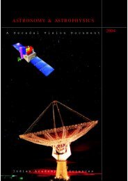
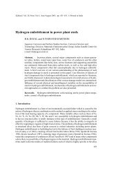
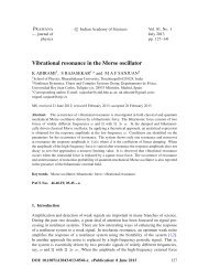
Figure 7.1 shows light scattering off a particle in solution or in vacuum. The incident light scatters
in all different directions. The intensity of the scattered light depends on the polarizability (to
be defined later) and the polarizability depends on the molecular weight. This property of light
scattering makes it a valuable tool for measuring molecular weight.
Because the intensity of scattered light depends on molecular weight of the particle, light
scattering will depend on weight average molecular weight. This result contrasts to colligative
properties, such as osmotic pressure, which only depended on number of particles and therefore
gave the number average molecular weight. Besides molecular weight dependence, light scattering
also has a direct dependence on particle size. For polymer solutions, this dependence on size can
be used to measure the radius of gyration of the polymer molecule. As with osmotic pressure, we
expect all light scattering experiments to be done in non-ideal solutions. Nonideality complicates
the data analysis, but, like osmotic pressure, allows you to determining a virial coefficient, A2.
In summary, light scattering experiments can be used to measure three things: weight average
molecular weight (MW ), mean-squared radius of gyration (〈s 2 〉), and the second virial coefficient
(A2 or Γ2).
To interpret light scattering experiments, we begin with a discussion of light scattering theories.
Classical light scattering theory was derived by Lord Rayleigh and is now called Rayleigh theory.
Rayleigh theory applies to small particles. By small particles, we mean particles whose size is much
less than λ or the wavelength of the light that is being scattered. By “much less” we mean
� 〈s 2 〉 < λ/20 (7.1)
Because visible light has λ between 4000˚A and 8000˚A, we need the root mean squared radius of
gyration � 〈s 2 〉 < 200 to 400˚A. Many polymers will violate this criterion and the light scattering
results will have to be corrected for large particle size effects.
89

90 CHAPTER 7. LIGHT SCATTERING
Incident Light
Scattered
Light
Figure 7.1: Scattering of incident light off a particle in solution or in vacuum.
A light scattering theory known as the Rayleigh-Gans theory was developed to extend Rayleigh
theory to particles that are not optically small. The correction method involves extrapolation
techniques that extrapolate light scattering intensity to zero scattering angle. This correction
technique is important for analyzing results on polymer solutions.
Analysis of osmotic pressure experiments requires extrapolation techniques to account for non-
ideal solutions. In light scattering there are two non-ideal effect — nonideal solutions and large
particle size effects. Thus, analysis or deconvolution of light scattering data requires two extrapo-
lations. One is an extrapolation to small particle size to remove the large particle size effect. The
other is an extrapolation to zero concentration to remove the effect of non-ideal solutions. The slope
of the first extrapolation gives the mean squared radius of gyration (〈s 2 〉). The slope of the second
extrapolation gives the second virial coefficient (A2). The intercept of the two extrapolations gives
the weight average molecular weight (MW ).
7.2 Rayleigh Theory
We begin by describing the theory for light scattering off a small particle in an ideal solution. Light
is an electromagnetic field. At the origin the field is time dependent and described by:
Ez = E0 cos
� �
2πct
where E0 is the amplitude of the electric field, c is the speed of light, and λ is the wavelength of
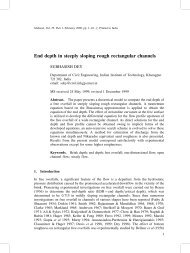
light. The subscript z on E means we are considering plane polarized light with the light polarized
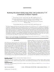
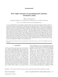
along the z axis. An incident beam of light polarized in the z direction is shown in Fig. 7.2.
If the particle at the origin in Fig. 7.2 is polarizable, the incident electric field will induce a
dipole moment in that particle. The magnitude of the dipole moment is proportional to the field.
λ
(7.2)

7.2. RAYLEIGH THEORY 91
Incident Polarized Light
z
Figure 7.2: Plane polarized light polarized in the z direction and incident on a small particle.
The proportionality constant is called the polarizability — αp. The higher a particle’s polarizability
the higher will be the magnitude of the dipole moment induced by a given electromagnetic field.
The dipole moment is
� �
2πct
p = αpE0 cos
λ
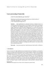
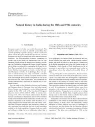
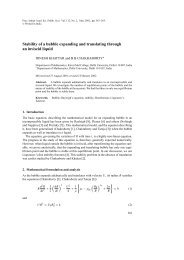
The induced dipole moment will radiate light in all directions. We consider observing the radiated
or scattered light at a distance r from the origin along a line that makes an angle θz with the z
axis (see Fig. 7.3). The scattered light field will be proportional to (1/c 2 )(d 2 p/dt 2 ). The second
derivative of p is the acceleration of the charge on the dipole moment. To include spatial effects,
the scattered light is also proportional to 1/r (electromagnetic fields die off as 1/r) and to sin θz
(the projection of the dipole moment on the observation direction). Combining all these effects,
the electric field for light scattered in the θz direction is
Es = 1 1
r c2 d2p 1
= −
dt2 c
2 αpE0
4π 2 c 2
rλ 2 sin θz cos
� �
2πct
Equipment that measures scattered light is typically only sensitive to the intensity of light. The
intensity of light is equal to the amplitude of the electromagnetic field squared. Thus, squaring the
amplitude of Es gives the scattered light intensity at r and θz:
Is = α 2 16π
pI0z
4
r2λ4 sin2 θz
where I0z is the intensity of the z polarized incident light.
I0z = E 2 0
λ
(7.3)
(7.4)
(7.5)
(7.6)

92 CHAPTER 7. LIGHT SCATTERING
Incident Polarized Light
z
Figure 7.3: Observation direction for light scattered off a particle at the origin in a direction that makes
an angle θz with respect to the z axis. The observation distance is r.
The above results are for incident light polarized in the z direction. Experiments, however, are
usually done with unpolarized light. We can account for unpolarized incident light by summing
the intensity of equal parts of incident light polarized in both the z direction and the y direction.
The incident intensity becomes
and the intensity of scattered light becomes
θz
I0 = 1
2 I0z + 1
2 I0y
Is = 1
2 Isz + 1
2 Isy
8π
= I0
4α2 p
r2λ4 � 2
sin θz + sin 2 �
θy
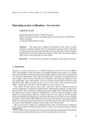
where θy is the angle the observation direction makes with the y axis. Scattering of unpolarized
light is illustrated in Fig. 7.4.
By geometry the θz and θy terms can be related to the angle θx that the observation direction
makes with the x axis (see Fig. 7.4). This angle will simply be referred to as θ. Because the sum
of the direction cosines is 1:
the geometric result is easily derived to be
r
(7.7)
(7.8)
cos 2 θx + cos 2 θy + cos 2 θz = 1 (7.9)
sin 2 θz + sin 2 θy = 1 + cos 2 θ (7.10)
We now have the scattered light intensity for scattering off a single particle. For scattering off n
moles of particles or nL particles (L is Avagadro’s number) in a dilute solution of volume V , the

7.3. IDEAL POLYMER SOLUTIONS WITH SMALL PARTICLES 93
Incident Unpolarized Light
z
Figure 7.4: Scattering of unpolarized light is analyzed by considering scattering of incident light polarized
in both the z and y directions.
scattered intensity at θ is:
i 0 θ
I0nL 8π
=
V
4α2 p
r2λ4 � � 2
1 + cos θ
The superscript 0 on the i indicates that this is scattering due to small molecules.
θ
(7.11)
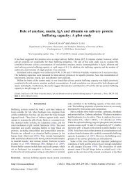
The light scattering intensity depends on scattering angle. The shape of the diagram is deter-
mined by the (1 + cos 2 θ) term. A plot of this term is given in Fig. 7.5. The maximum scattering
intensity is at θ = 0. The minimum scattering intensity is at θ = 90. The scattering intensity for
forward scattering is equal to the intensity for back scattering at the corresponding angle. In other
words, the scattering intensity at angle θ is equal to the scattering intensity at angle 180 − θ.
As a function of λ, the scattered intensity is proportional 1/λ 4 . This strong wavelength depen-
dence makes short wavelength light scatter more than long wavelength light. This effect explains
why the sky is blue. Short wavelength or blue light scatters the most. Normally we do not look
at the sun and θ is not zero. When θ is not zero you see the scattered light or the blue light. At
sunset you normally do look in the direction of the sun and θ is zero or near zero. Because blue
light is scattered away, you are left with the red light and sunsets appear red.
7.3 Ideal Polymer Solutions with Small Particles
For practical results, we need to make a connection between the scattering intensity derived in the
previous section and molecular weight of the polymer particles in solution. The connection arises
because polarizability depends on molecular weight. First, the polarizability can be thought of as

94 CHAPTER 7. LIGHT SCATTERING
1
-2 -1 1 2
-0.5
-1
Figure 7.5: Shape of the scattering intensity as a function of scattering angle for scattering off a small
particle.
a difference in the index of refraction between the polymer and the solvent. In other words light
scattering only occurs in mediums that have an inhomogeneous index of refraction. Specifically,
the polarizability of particles at concentration c is
αp = n0cV dn0
2πnL dc
θ
(7.12)
where n0 is the index of refraction of the solution and dn0/dc is the concentration dependence of
the index of refraction. Note that if the index of refraction of the solvent and of the polymer are
the same then dn0/dc will be zero and there would be no polarizability and therefore no scattered
light. Writing c as nM/V (in units of g/ml) yields
αp = n0M
2πL
and substituting into the scattered light intensity gives (where we also replace n/V by c/M):
i 0 θ
I0
= 2π2
r 2 λ 4
n 2 0
L
dn0
dc
� �2 dn0
Mc
dc
� 1 + cos 2 θ �
(7.13)
(7.14)
In a given scattering experiment, I0 and r will be fixed and we will measure i0 θ . These measured
quantities can be combined into one quantity called the Rayleigh ratio — R0 θ :
R 0 θ = r2 i 0 θ
I0
(7.15)
The advantage of the Rayleigh ratio is that it is independent of the incident light intensity and
the distance to the scattered light detector (i.e., independent of I0 and r). From the scattering
equation, the Rayleigh ratio can be written as:
R 0 θ
= KMc (7.16)

7.4. NON-IDEAL POLYMER SOLUTIONS 95
where
K = 2π2 n 2 0
λ 4 L
� �2 dn0 �1 � 2
+ cos θ
dc
(7.17)
The constant K depends only on the solvent properties, on λ, and on θ. K is therefore a system
constant that is independent of the concentration of the solution and the molecular weight of the
polymer.
For a dilute, polydisperse polymer solution, the total Rayleigh ratio can be written as a sum of
the Rayleigh ratios for scattering of polymers of each possible molecular weight:
�
= K
or
Kc
R 0 θ
=
R 0 θ
�
i ci
�
i ciMi
=
i
ciMi
�
i NiMi
�
i NiM 2 i
= 1
MW
(7.18)
(7.19)
The Rayleigh ratio for an ideal polymer solution with small particles is thus directly related to the
weight average molecular weight (MW ).
7.4 Non-Ideal Polymer Solutions
As done with osmotic pressure, the possibility of non-ideal solutions is handled by adding virial
coefficients and concentration terms to the ideal result. Thus expanding Kc/R 0 θ gives
Kc
R 0 θ
= 1
MW
+ 2A2c + 3A3c 2 + · · · (7.20)
The virial coefficients A2 and A3 are the same as the virial coefficients we discussed in osmotic
pressure theory. The factors of 2, 3, etc., come from the thermodynamic theory of fluctuations
which can be used to show that
Kc
R 0 θ
where π is osmotic pressure. In a virial expansion
= 1 ∂π
RT ∂c
(7.21)
π = RT
c + RT A2c 2 + RT A3c 3 + · · · (7.22)
MN
To convert to the light scattering experiment, the MN in the π expression must be changed to MW .
The only difference between the A2 in osmotic pressure and the A2 in light scattering is that the
light scattering A2 is formally a weight-average virial coefficient. Besides that difference, the light
scattering A2 gives similar information, notably information about the quality of the solvent.
Typically, we will ignore terms beyond the second virial coefficient. Then Kc/R 0 θ
be linear in c. From experiments we can plot Kc/R 0 θ
is predicted to
as a function of c. The slope will give the second
virial coefficient (slope = 2A2) and the intercept will give the molecular weight (intercept = 1/MW ).
This extrapolation, however, ignores any possible large particle size effects The extrapolated MW
will therefore be in error. The next section considers how to correct for large particle size.

96 CHAPTER 7. LIGHT SCATTERING
Scattering from different
parts of the particle
Path length difference
causes destructive interference
Figure 7.6: Scattering of light of two different parts of a large polymer molecule.
7.5 Large particles
If a particle is not small compared to the wavelength of light, the light can scatter from different
parts of the particle. Fig. 7.6 shows a large polymer that is scattering light. Light scattering
from different parts of the particle will reach the detector by traveling different path lengths. The
difference in path lengths can lead to destructive interference that reduces the intensity of the
scattered light. The net effect is that the scattering diagram for large particles is reduced in
intensity from the scattering diagram for small particles (see Fig. 7.5).
The amount of intensity reduction or the amount of destructive interference depends on the
scattering angle. At θ equal to zero, the path lengths will always be identical. With identical path
lengths, there will be no destructive interference. In other words at θ = 0, the intensity of scattered
light will be identical to i0 θ . At θ not equal to zero there will be destructive interference. As θ
increases, the interference will increase reaching a maximum and θ = 180◦ . A comparison of the
scattering diagrams for large particles vs. small particles is given in Fig. 7.7. The large particle
scattering diagram shows the effect of large particles and now shows asymmetry in scattering; i.e.,
the back scattering intensity is much reduced from the forward scattering intensity.
To correct for large particles, we merely need to do the light scattering experiments at zero
scattering angle (θ = 0). Unfortunately, these experiments cannot be done. At θ = 0 most light
will be transmitted light that is not scattered. The transmitted light will swamp the scattered
light preventing its measurement. Because scattered light and transmitted light have the same
wavelength, there is no way to distinguish between them. Instead, we must do experiments at
θ > 0 and extrapolate to θ = 0. We thus do a second extrapolation, an extrapolation to zero
scattering angle.
To develop an extrapolation method, we define a new function, P (θ), that describes the large

7.5. LARGE PARTICLES 97
Small
Particles
1
-2 -1 1 2
-0.5
-1
Large
Particles
Figure 7.7: Scattering diagrams for both small particles and large particles.
particle size effect. P (θ) is the ratio between the actual scattering (iθ) and the scattering that
would occur off small particles (i 0 θ )
P (θ) = iθ
i 0 θ
= Rθ
R 0 θ
θ
(7.23)
From the above discussions we know that P (0) = 1 (there is no effect at zero scattering angle)
and P (θ) < 1 for all other θ (destructive interference can only cause a reduction in intensity). The
larger effect on back scattering than on forward scatter means that P (θ < 90) > P (180 − θ).
First consider an ideal solution. The measured Rayleigh ratio, written as Rθ, includes the large
particle size effect. Using P (θ) we can write Rθ = P (θ)R0 θ . The key measured quantity becomes
Kc
Rθ
= Kc
P (θ)R 0 θ
1
=
MW P (θ)
(7.24)
The second equality follows from the previously derived ideal solution result with small particles.
To use this equation, we need some information about P (θ). That information can sometimes be
derived by theoretical analysis of large-particle scattering. Fortunately, some theoretical results are
available for scattering off a large random coil. The results are accurate as long as the particle size
is not too large. Instead of requiring � 〈s 2 〉 < λ/20 as done before for small particles, we can use
the theoretical result to handle particles with � 〈s 2 〉 < λ/2. For scattering with visible light we
now can use � 〈s 2 〉 < 2000˚A to 4000˚A. Most polymers fall within or below this range and thus we
can derive effective extrapolation methods for scattering off polymer molecules.
The theoretical result for P (θ) is
1 16π2
= 1 +
P (θ) 3λ2 〈s2 2 θ
〉 sin + · · · (7.25)
2
The “· · ·” means that there are higher order terms in sin(θ/2). Those terms are normally assumed
to be negligible. For a polydisperse polymer, the scattering intensity as a function of scattering

98 CHAPTER 7. LIGHT SCATTERING
angle becomes
Kc
Rθ
= 1
MW
�
1 + 16π2
3λ2 〈s2 2 θ
〉w sin
2
�
(7.26)
Note we have changed 〈s 2 〉 to 〈s 2 〉w, the weight average radius of gyration squared. In terms of the
various polymer weights, the relevant radius of gyration squared is
〈s 2 〉w =
�
i NiMi〈s 2 〉i
�
i NiMi
= �
i
wi〈s 2 〉i
where 〈s 2 〉i is the average squared radius of gyration for polymers with molecular weight Mi
(7.27)
To find weight-average molecular weight (MW ) in ideal solutions, we truncate 1/P (θ) after the
sin 2 (θ/2) term and plot Kc/Rθ as a function of sin 2 (θ/2). That plot should be linear. The intercept
will give the molecular weight:
intercept = 1
MW
The slope divided by the intercept will give the radius of gyration
slope/intercept = 16π2 〈s 2 〉w
3λ 2
7.6 Light Scattering Data Reduction
(7.28)
(7.29)
To handle both non-ideal solutions and large particle effects, we need to do two extrapolations.
First, we introduce non-ideal solution effects into the large particle analysis in the previous section.
Instead of using P (θ) to correct the ideal solution result, we use it to correct the non-ideal solution
result. Thus the actually measured Kc/Rθ is
Kc
Rθ
= Kc
P (θ)R 0 θ
�
1
=
MW
�
1
+ 2A2c
P (θ)
(7.30)
where we have truncated the non-ideal solution result to a single virial coefficient. Inserting the
theoretical result for P (θ) truncated after the sin 2 (θ/2) term gives
�
Kc 1
=
Rθ
MW
� �
+ 2A2c 1 + 16π2
3λ2 〈s2 �
2 θ
〉w sin
2
(7.31)
A set of light scattering experiments consists of measure Kc/Rθ for various concentrations and
at various scattering angles. To get MW , we do two extrapolations. First, plotting Kc/Rθ as a
function of sin 2 (θ/2) at constant c gives a straight line with the following slope and intercept:
slope =
intercept =
� 1
MW
� 1
MW
�
16π2 + 2A2c
3λ2 〈s2 〉w
�
+ 2A2c
(7.32)
(7.33)

7.6. LIGHT SCATTERING DATA REDUCTION 99
Kc
R θ
c=0 c1 c2
c3 c4
c5
θ6
θ5
θ1
θ=0
sin 2 θ + kc
2
θ2
θ4
θ3
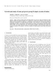
Figure 7.8: Typical Zimm plot. The experimental data points are at the grid intersection points except
along the θ = 0 and c = 0 lines.
Next we plot the intercepts of the first plots as a function of concentration. The resulting plot
should be a straight line with
slope = 2A2 (7.34)
intercept =
1
(7.35)
The slope and intercept of the second line gives us MW and A2. Substituting these results into the
slope of the first line allows us to find 〈s 2 〉w. We could achieve similar results by first plotting as a
function of concentration and then plotting the intercept of those plots as a function of sin 2 (θ/2).
The above analysis assumes that all c’s are low enough such that the concentration dependence
is linear in concentration and only requires the second virial coefficient. It also assumes all scattering
angles are low enough that terms higher than the sin 2 (θ/2) can be neglected. Both these conditions
MW
are easy to satisfy for light scattering with polymer solutions.
The analysis method described above is easy to do in a personal computer. When light scatter-
ing techniques were first developed, however, computers were not available and the numerous linear
fits were tedious. To avoid the tedium the Zimm plot was developed. In the Zimm plot technique,
you plot Kc/Rθ versus sin 2 (θ/2) + kc where k is a constant. k is chosen to spread out the plot and
give equal weights to each variable. For example sin 2 (θ/2) is always less than 1 or has a maximum
of 1. The range in kc should also go from 0 to 1 or kcmax = 1 which means a good k might be
1/cmax where cmax is the maximum concentration used. A typical Zimm plot is given in Fig. 7.8.
Plotting all Kc/Rθ points on a Zimm plot should result in a grid such as the one shown in

100 CHAPTER 7. LIGHT SCATTERING
Fig. 7.8. There will be experimental points at all grid points except along the lower line (the θ = 0
line) and the left-most line (the c = 0) line. Connecting all the grid lines and extrapolating to the
lower-left corner, the intercept point gives the molecular weight (intercept = 1/MW ). Incorporating
the k constant, the Zimm plot is plotting
�
Kc
=
1
+ 2A2
k kc
� �
1 + 16π2
3λ2 〈s2 �
2 θ
〉w sin
2
Rθ
MW
(7.36)
The slopes of the two directions in the parallelogram have physical meaning. The lines labeled θ1,
θ2, etc., are lines at constant θ. Inspection of the Zimm equation shows that the slopes of these
lines are:
slope of the contant θ lines = 2A2
k
�
1 + 16π2
3λ2 〈s2 2 θ
〉w sin
2
�
(7.37)
Notice that these slopes are a function of θ. Thus the slope of the θ = 0 line and the θ5 (or any θi
line) are different. In other words the Zimm plot is not actually a parallelogram. The lines labeled
c1, c2, etc., are lines at constant concentration. Inspection of the Zimm equation shows that the
slopes of these lines are:
�
1
slope of the constant c lines =
MW
�
16π2 + 2A2c
3λ2 〈s2 〉w
(7.38)
Notice that these slopes are a function of c. Thus the slope of the c = 0 line and the c5 (or any
ci line) are different. In other words the Zimm plot is not actually a parallelogram. The slopes
of constant θ and constant c lines both depend on A2 and on 〈s 2 〉w. The slopes of the constant θ
lines are mostly sensitive to A2. The slopes of the constant c lines are mostly sensitive to 〈s 2 〉w.
Because A2 and 〈s 2 〉w are independent physical quantities, it is possible to get Zimm plots that
are inverted from the plot in Fig. 7.8. If A2 increases and/or 〈s 2 〉w decreases, it is possible for the
steeper lines to be the constant θ lines and for the shallower lines to be the constant c lines.