Newton's law of cooling revisited - Cartan

More documents

Recommendations

Info

1066 M Vollmer Figure 1. Whenever an object is placed in an environment of different temperature, there will be a net energy transfer due to thermal radiation due to emission as well as absorption of radiation by the object. the current of the fluid is due to temperature and, hence, density differences in the fluid. In forced convection, the current of the fluid is due to external forces/pressure. Theoretically, convective heat transfer is modelled using dimensionless numbers such as the Nusselt number, the Prandtl number, the Grashof number and the Rayleigh number [1]. These depend on the Reynolds number which defines the kind of flow (laminar versus turbulent). Therefrom it follows that αConv depends on viscosity, thermal conductivity etc and also nonlinearly on the temperature difference, i.e. αConv ∼ �T x . The exact power x depends on the flow conditions, e.g. for free convection around a horizontal plate, it changes from x = 0.25 for laminar flow to 0.33 for turbulent flow [1]. Typical values for free-convective heat-transfer coefficients of gases above solids are cited to range between 2 and 25 W (m 2 K) −1 , the exact value depending on flow conditions, wind speed and moisture of the surface; for liquids they can be in the range 50–1000 W (m 2 K) −1 . Here, we neglect any effects of latent heat associated with convective heat transfer. 2.3. Radiation The emission of thermal radiation by an object is usually expressed as the product of a material property, the emissivity ε and the blackbody radiation due to the object temperature T (e.g. [1, 2, 27–29]. For many objects (in particular all studied in this work), the emissivity can be assumed to be independent of wavelength, i.e. having a constant value �0.85. In any realistic situation, an object of temperature Tobj is surrounded by other objects of background temperatures Tsurr. For simplicity, we assume an object (figure 1) which is completely surrounded by an enclosure of constant temperature (if the surrounding consists of objects with different temperatures, one needs to compute the respective view factors to find the net radiation transfer [1, 2]). In addition to the emission of radiation from the object there is radiation from the surroundings incident onto the object. This finally leads to a net energy transfer from the object with the surface area A to the surroundings ˙QRad = ε · σ · A · � T 4 � 4 obj − Tsurr . (3) Since any quantitative analysis concerning the heat transfer is much easier for linear temperature differences, it is customary to approximate the radiative contribution also with
Newton’s law of cooling revisited 1067 a linear equation. This makes sense, if temperature differences are small (Tobj ≈ Tsurr, i.e. �T ≪ Tsurr, Tobj), since in this case � 4 Tobj − T 4 � surr = kappr(T ) · (Tobj − Tsurr), (4) where kappr (T) ≈ 4T 3 Surr .UsingαRad = ε · σ · kappr, equation (3) can be rewritten as ˙QRad = αRad · A · (Tobj − Tsurr), (5) which is of the same type as the heat-transfer equations for conduction and convection. 3. Conduction within solids: the Biot number In the experiments described below, information about the temperatures of solid objects will be gained from the surface temperatures of these objects. It is important to know how these surface temperatures are related to average temperatures in order to correctly model the cooling process. Consider a solid, which is between two fluids of different but constant temperatures T1 and T2. Assuming steady state conditions the heat flows due to conduction, convection and radiation will lead to a spatial temperature distribution within the object. It is possible to get some idea on this temperature distribution within the solid by using the so-called Biot number Bi. Bi = αConv αCond = αConv . (6) λ/s The Biot number is a dimensionless quantity, usually describing the ratio of two adjacent heat-transfer rates. In the present case, it describes the ratio of the outer heat flow from the surface to the surrounding, characterized by the convective heat-transfer coefficient αConv at the surface, and the inner heat flow within the object characterized by the conductive heat-transfer coefficient αcond = (λ/s). For Bi ≫ 1, the outer heat flow is much larger than the inner heat flow. Obviously, this will result in a strong spatial variation of internal temperature within the object. This is typical for walls of buildings. If however, Bi ≪ 1, the internal heat flow is much larger than the heat loss from the surface. Therefore, there will be temperature equilibrium within the object, i.e. a homogeneous temperature distribution within the solid and the drop at the boundary of the object to the surrounding fluid is much larger [1]. 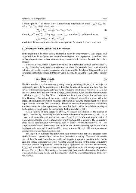As an example of time-dependent effects, we discuss the situation of the cooling of objects. Consider e.g. an initially hot one-dimensional object of temperature Tobj which is in contact with surroundings of lower temperature. Figure 2 gives a schematic representation of temperature within the object as a function of time for different Biot numbers. The temperature drops outside the boundaries were omitted here for clarity. For the Biot numbers
Page 1 and 2: IOP PUBLISHING EUROPEAN JOURNAL OF
Page 3: Newton’s law of cooling revisited
Page 7 and 8: Newton’s law of cooling revisited

Newton's law of cooling revisited - Cartan

Create successful ePaper yourself

Delete template?

Save as template?