Newton's law of cooling revisited - Cartan
Newton's law of cooling revisited - Cartan
Newton's law of cooling revisited - Cartan

Create successful ePaper yourself
Turn your PDF publications into a flip-book with our unique Google optimized e-Paper software.
1076 M Vollmer<br />
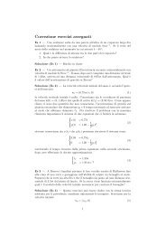
Figure 9. Set up for <strong>cooling</strong> cans and bottles <strong>of</strong> liquids in a freezer.<br />
everyday objects and situations, relatively small temperature differences could be realized.<br />
These were expected to be accurately described by Newton’s <strong>law</strong> <strong>of</strong> <strong>cooling</strong>. Second, we<br />
studied metal cubes as were treated in the theoretical analysis as model systems due to their<br />
simple geometry. Experimentally, we could realize temperature differences up to 140 K.<br />
Third, in order to achieve higher initial temperature differences, we used halogen light bulbs<br />
for temperature differences <strong>of</strong> up to 300 K. All temperatures were measured using IR imaging<br />
(see [29]). The fridge and the metal cube experiments could also easily be measured using<br />
conventional thermocouples; however, the much faster drop in temperature in the light bulb<br />
experiments requires fast contactless temperature measurements such as with an IR camera or<br />
a pyrometer. Nowadays rather cheap and small IR camera systems are available (some cost less<br />
than 3000€ for 80 × 80 pixels), therefore all experiments may be suitable for undergraduate<br />
student laboratories.<br />
6.1. Liquids in refrigerator: �T � 50 K<br />
The daily life experiences <strong>of</strong> <strong>cooling</strong> are <strong>of</strong>ten related to fridges or freezers. As two examples<br />
we measured the <strong>cooling</strong> <strong>of</strong> cans and bottles filled with water (or other liquids) as a function<br />
<strong>of</strong> time for different <strong>cooling</strong> methods, using first a conventional fridge with a low temperature<br />
<strong>of</strong> 6 ◦ C, second a (∗∗∗) freezer with a low temperature <strong>of</strong> −21 ◦ C to –22 ◦ C and third an<br />
air convection cooler set to a low temperature <strong>of</strong> −5.5 ◦ C. As an example, figure 9 depicts<br />
the experimental set-up for the freezer. The Biot numbers for cans and bottles (see table 1)<br />
were below 0.1; therefore, we assumed the surface temperatures to be a useful measure for<br />
the average temperatures <strong>of</strong> the objects (it was shown that the actual average temperatures and<br />
the ones assuming Bi ≪ 1 only lead to deviations <strong>of</strong> 2% between the real average temperature<br />
and the one based on the approximation for geometric forms <strong>of</strong> sphere, cylinder, prisms and<br />
cube [2]).<br />
The <strong>cooling</strong> power <strong>of</strong> the systems is expected to be quite different. The conventional fridge<br />
and the freezer both have objects surrounded by still air, since the temperature differences are<br />
usually too low to generate natural convection. Hence, the heat-transfer coefficients and the<br />
<strong>cooling</strong> time constants <strong>of</strong> both should be the same. However, the refrigerator has a smaller<br />
temperature difference than the freezer; therefore, the <strong>cooling</strong> power <strong>of</strong> the freezer is larger and<br />
the effective <strong>cooling</strong> times (times to reach a certain low temperature upon <strong>cooling</strong>) are smaller