Newton's law of cooling revisited - Cartan

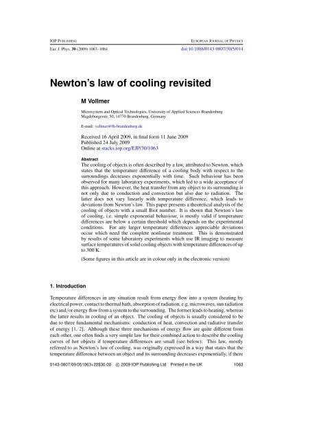
IOP PUBLISHING EUROPEAN JOURNAL OF PHYSICS 

Eur. J. Phys. 30 (2009) 1063–1084 doi:10.1088/0143-0807/30/5/014 

Newton’s law of cooling revisited 

1. Introduction 

M Vollmer 

Microsystem and Optical Technologies, University of Applied Sciences Brandenburg 

Magdeburgerstr. 50, 14770 Brandenburg, Germany 

E-mail: vollmer@fh-brandenburg.de 

Received 16 April 2009, in final form 11 June 2009 

Published 24 July 2009 

Online at stacks.iop.org/EJP/30/1063 

Abstract 

The cooling of objects is often described by a law, attributed to Newton, which 

states that the temperature difference of a cooling body with respect to the 

surroundings decreases exponentially with time. Such behaviour has been 

observed for many laboratory experiments, which led to a wide acceptance of 

this approach. However, the heat transfer from any object to its surrounding is 

not only due to conduction and convection but also due to radiation. The 

latter does not vary linearly with temperature difference, which leads to 

deviations from Newton’s law. This paper presents a theoretical analysis of the 

cooling of objects with a small Biot number. It is shown that Newton’s law 

of cooling, i.e. simple exponential behaviour, is mostly valid if temperature 

differences are below a certain threshold which depends on the experimental 

conditions. For any larger temperature differences appreciable deviations 

occur which need the complete nonlinear treatment. This is demonstrated 

by results of some laboratory experiments which use IR imaging to measure 

surface temperatures of solid cooling objects with temperature differences of up 

to 300 K. 

(Some figures in this article are in colour only in the electronic version) 

Temperature differences in any situation result from energy flow into a system (heating by 

electrical power, contact to thermal bath, absorption of radiation, e.g. microwaves, sun radiation 

etc) and/or energy flow from a system to the surrounding. The former leads to heating, whereas 

the latter results in cooling of an object. The cooling of objects is usually considered to be 

due to three fundamental mechanisms: conduction of heat, convection and radiative transfer 

of energy [1, 2]. Although these three mechanisms of energy flow are quite different from 

each other, one often finds a very simple law for their combined action to describe the cooling 

curves of hot objects if temperature differences are small (see below). This law, mostly 

referred to as Newton’s law of cooling, was originally expressed in a way that states that the 

temperature difference between an object and its surrounding decreases exponentially, if there 

0143-0807/09/051063+22$30.00 c○ 2009 IOP Publishing Ltd Printed in the UK 1063

1064 M Vollmer 

is no additional heating involved [3]. Many modern textbooks present this law in another way 

to describe the physics behind the exponential decrease by stating Newton’s law to mean that 

the heat transfer from an object to the surrounding is proportional to the respective temperature 

difference (e.g. [1], the very helpful comment by Bohren [3]; see also [4]). The respective 

time constant τ in the exponential function is characteristic for the object under study, i.e. it 

depends on its properties (heat capacity, size, geometry [5, 6]etc). 

In the last few decades, quite a number of publications dealt with Newton’s law of cooling. 

Some historical notes can be found in [7, 8]. The nearly endless discussions about Newton’s 

law of cooling may be summarized by the statement of O’Connell [9]: ‘Newton’s law of 

cooling is one of those empirical statements about natural phenomena that should not work, 

but does.’ Similarly, in 1969 it was stated that ‘there is no definitive body of experimental 

data which defines the limits within which reality conforms to the law’ and experiments 

using steady air flow around hot objects led to the conclusion that cooling in air proceeded 

geometrically (i.e. following exponential decay) up to 200 ◦C[7]. In detail, earlier work on Newton’s law of cooling dealt with 

– undergraduate lab experiments to demonstrate exponential cooling curves [10, 11], 

– comparison of the cooling of solids with Newton’s law [12], 

– the influence of a finite reservoir of lower temperature than the object (e.g. well-defined 

amounts of hot water surrounded by cold water) [13], 

– the mechanical equivalent of heat from Joule’s experiment [14], 

– the cooling of tea or coffee [15], 

– modelling the transient temperature distributions of metal rods heated at one side only 

[16], 

– measuring specific heats of solids and thermal conductivities [17–19], 

– the cooling of spherical objects (like fuel droplets) in a gas [20] 

– boundary conditions in studies modelling thermos [21], 

– the world record for creating the fastest ice cream using liquid nitrogen [22], 

– the cooling of incandescent lamp filaments [23] and 

– explanations concerning the relevant corrections for the heating curves of water [9]. 

In most papers, linearization for the radiative contribution of heat transfer was used in 

order to end up with Newton’s law. However, this is only justified for small temperature 

differences. In any case, one may expect that the strong nonlinearity of the radiative cooling 

processes should lead to deviations from the simple exponential behaviour. 

Although this nonlinearity due to radiative processes was often recognized (e.g. [3, 4, 

8, 24]), linearization was often considered to be an appropriate approximation. This was 

motivated by the fact that experimental investigations usually dealt with the low temperaturedifference 

regime of say �T < 50 K, where notable deviations from the exponential decrease 

due to the linear behaviour were not observed. (Notable deviations in the context of this paper 

mean that actual values for the temperature differences deviate from expectation according to 

Newton’s law, i.e. a simple exponential, by say 5% or more.) In particular, an extensive study 

of the easiest student lab experiments like the cooling of flasks filled with hot water never 

showed any deviations from exponential cooling for �T < 55 K [25, 26]. 

Therefrom several interrelated questions arise: namely (i) what is the magnitude of 

deviations? (ii) is it possible to define a range of validity for Newton’s law of cooling? and 

(iii) can these deviations be easily observed experimentally? 

In the following, all three questions will be addressed. First, a brief theoretical analysis 

of heat-transfer modes for cooling objects will be given. Second, in order to simplify the 

theoretical analysis and to properly describe simple experiments, we will discuss the so-called

Newton’s law of cooling revisited 1065 

Biot number. Emphasis will be on objects with a small Biot number. Third, the assumptions 

underlying Newton’s law of cooling will be discussed. Fourth, the correct theoretical treatment 

of the radiative heat transfer leads to deviations from Newton’s law which will be discussed 

upon variation of a number of parameters. It will be demonstrated that the temperature range 

where Newton’s law is valid does sensitively depend on the relative contributions of convective 

versus radiative heat transfer. Finally, experimental results with temperature differences �T 

of up to 300 K will be presented which clearly verify the theoretically predicted deviations 

from Newton’s law of cooling. 

The problem as well as some experiments seem to be appropriate for undergraduate 

physics courses. 

2. The basic heat-transfer modes: conduction, convection and radiation 

Temperature differences in any situation result from energy flows into a system and energy 

flows from a system to the surrounding. The former leads to heating, whereas the latter 

results in cooling of an object. In thermodynamics, any kind of energy flow which is due to 

a temperature difference between a system and its surroundings is usually called heat flow 

or heat transfer. In physics, one usually distinguishes three kinds of heat flow: conduction, 

convection and radiation. 

2.1. Conduction 

Conduction refers to the heat flow in a solid or fluid (liquid or gas) which is at rest. Conduction 

of heat within an object, e.g. a one-dimensional wall, is usually assumed to be proportional 

to the temperature difference T1 − T2 on the two sides of the object as well as the surface 

area A of the object. This follows from the left-hand side of equation (1) by approximating 

dT/ds ≈ �T/s: 

˙QCond = λ · A · dT 

ds 

≈ λ 

s · A · (T1 − T2) = αCond · A · (T1 − T2). (1) 

The heat-transfer coefficient within the object is defined as αCond = λ 

, where λ is the 

s 

thermal conductivity and s is a measure for the object size. For the one-dimensional wall 

it would be the wall thickness. The heat-transfer coefficient αCond describes heat transfer in 

W(m2K) −1 . Hence the heat flux through the wall ˙QCond in W gives the energy flow per 

second through the wall of the surface area A if the temperature difference between the inner 

and outer surfaces is given. Typical values of heat-transfer coefficients for s = 10 cm ‘wall 

thickness’ for pure metals are of the order of 1000 W (m2 · K) −1 , building materials such as 

concrete, stones or glass range between 5 and 20 W (m2 · K) −1 , water has 0.6 W (m2 · K) −1 , 

and insulating foams or gases range between 0.2 and 0.5 W (m2 · K) −1 . 

2.2. Convection 

In general, convection refers to the heat flow between a solid and a fluid in motion. The 

energy flow ˙QCond per second from the surface of an object with temperature T1 into a fluid 

of temperature T2 due to convection is usually assumed to follow a law similar to the one of 

conduction 

˙QConv = αConv · A · (T1 − T2). (2) 

The heat-transfer coefficient for convection depends on the nature of the motion of the fluid, 

on the fluid velocity and on temperature differences. One distinguishes free convection where


Figure 1. Whenever an object is placed in an environment of different temperature, there will be 

a net energy transfer due to thermal radiation due to emission as well as absorption of radiation by 

the object. 

the current of the fluid is due to temperature and, hence, density differences in the fluid. In 

forced convection, the current of the fluid is due to external forces/pressure. Theoretically, 

convective heat transfer is modelled using dimensionless numbers such as the Nusselt number, 

the Prandtl number, the Grashof number and the Rayleigh number [1]. These depend on the 

Reynolds number which defines the kind of flow (laminar versus turbulent). Therefrom it 

follows that αConv depends on viscosity, thermal conductivity etc and also nonlinearly on the 

temperature difference, i.e. αConv ∼ �T x . The exact power x depends on the flow conditions, 

e.g. for free convection around a horizontal plate, it changes from x = 0.25 for laminar flow 

to 0.33 for turbulent flow [1]. 

Typical values for free-convective heat-transfer coefficients of gases above solids are cited 

to range between 2 and 25 W (m 2 K) −1 , the exact value depending on flow conditions, wind 

speed and moisture of the surface; for liquids they can be in the range 50–1000 W (m 2 K) −1 . 

Here, we neglect any effects of latent heat associated with convective heat transfer. 

2.3. Radiation 

The emission of thermal radiation by an object is usually expressed as the product of a material 

property, the emissivity ε and the blackbody radiation due to the object temperature T (e.g. 

[1, 2, 27–29]. For many objects (in particular all studied in this work), the emissivity can be 

assumed to be independent of wavelength, i.e. having a constant value �0.85. 

In any realistic situation, an object of temperature Tobj is surrounded by other objects 

of background temperatures Tsurr. For simplicity, we assume an object (figure 1) which is 

completely surrounded by an enclosure of constant temperature (if the surrounding consists of 

objects with different temperatures, one needs to compute the respective view factors to find 

the net radiation transfer [1, 2]). 

In addition to the emission of radiation from the object there is radiation from the 

surroundings incident onto the object. This finally leads to a net energy transfer from the 

object with the surface area A to the surroundings 

˙QRad = ε · σ · A · � T 4 � 4 

obj − Tsurr . (3) 

Since any quantitative analysis concerning the heat transfer is much easier for linear 

temperature differences, it is customary to approximate the radiative contribution also with


a linear equation. This makes sense, if temperature differences are small (Tobj ≈ Tsurr, i.e. 

�T ≪ Tsurr, Tobj), since in this case 

� 4 

Tobj − T 4 � 

surr = kappr(T ) · (Tobj − Tsurr), (4) 

where kappr (T) ≈ 4T 3 Surr .UsingαRad = ε · σ · kappr, equation (3) can be rewritten as 

˙QRad = αRad · A · (Tobj − Tsurr), (5) 

which is of the same type as the heat-transfer equations for conduction and convection. 

3. Conduction within solids: the Biot number 

In the experiments described below, information about the temperatures of solid objects will 

be gained from the surface temperatures of these objects. It is important to know how these 

surface temperatures are related to average temperatures in order to correctly model the cooling 

process. 

Consider a solid, which is between two fluids of different but constant temperatures T1 

and T2. Assuming steady state conditions the heat flows due to conduction, convection and 

radiation will lead to a spatial temperature distribution within the object. It is possible to get 

some idea on this temperature distribution within the solid by using the so-called Biot number 

Bi. 

Bi = αConv 

αCond 

= αConv 

. (6) 

λ/s 

The Biot number is a dimensionless quantity, usually describing the ratio of two adjacent 

heat-transfer rates. In the present case, it describes the ratio of the outer heat flow from the 

surface to the surrounding, characterized by the convective heat-transfer coefficient αConv at the 

surface, and the inner heat flow within the object characterized by the conductive heat-transfer 

coefficient αcond = (λ/s). For Bi ≫ 1, the outer heat flow is much larger than the inner heat 

flow. Obviously, this will result in a strong spatial variation of internal temperature within the 

object. This is typical for walls of buildings. If however, Bi ≪ 1, the internal heat flow is much 

larger than the heat loss from the surface. Therefore, there will be temperature equilibrium 

within the object, i.e. a homogeneous temperature distribution within the solid and the drop at 

the boundary of the object to the surrounding fluid is much larger [1]. 

As an example of time-dependent effects, we discuss the situation of the cooling of 

objects. Consider e.g. an initially hot one-dimensional object of temperature Tobj which is in 

contact with surroundings of lower temperature. Figure 2 gives a schematic representation of 

temperature within the object as a function of time for different Biot numbers. The temperature 

drops outside the boundaries were omitted here for clarity. For the Biot numbers


(a) 

(c) 

(b) 

Figure 2. Schematic temperature distributions within solid objects upon cooling as a function of 

the increasing Biot number (Bi = 0, Bi = 0(1), i.e. of the order of unity, Bi ≫ 1). For finite 

object temperature, there is an additional temperature drop at the boundary to the surrounding 

fluid, which was omitted here. The intermediate situation (b) depicts also the differences between 

surface, centre and average temperature of a sphere. 

Table 1 gives a summary of Biot numbers for some objects used in our experiments (see 

below). For small objects of metal the condition Bi < 0.1 is usually fulfilled. The same holds 

for cans/bottles filled with water for both the liquid inside and the walls of the container. This 

means that we can simplify the models by assuming thermal equilibrium within the objects, 

i.e. by describing the cooling process with average temperatures of the objects. In the case of 

bottles/cans, any internal convection of the water would increase λ, hence decrease Bi further. 

4. Simplified model for cooling of objects for Bi ≪ 1 

Consider a homogeneously heated object, which can be described by a small Biot number, i.e. 

an average temperature is sufficient to characterize the cooling of the object. If the object is 

just placed in air, we assume typical values for heat-transfer coefficients for free convection 

(solids to gases) in the range 2–25 W (m 2 K) −1 . Supposing an initial temperature Tinit of the 

objects, energy conservation requires that any heat loss will lead to a decrease of the thermal


Table 1. Some material properties of objects and respective Biot numbers. 

αConv λ (W αCond = λ/s Biot 

Object Material(s) (W/(m 2 K) −1 ) s in m (m · K) −1 ) (W(m 2 K) −1 ) number 

Metal cubes Aluminium, paint 2–25 20–60 × 10 −3 220 11 000–3670 220 000 ≪1 

can (0.5 l) water inside 3.3 × 10 −2 radius 0.6 18.2 ≈0.1 

Light bulbs Glass 2–25 1 × 10 −3 ≈1 1000 0.002–0.025 

Bottle (0.5 l) Glass with 2 ≈3 × 10 −3 ≈1 333 ≈0.006 

in fridge water inside 3.3 × 10 −2 radius 0.6 18.2 ≈0.1 

energy of the object, i.e. 

mc dTobj 

dt =−˙QConv − ˙QRad, (7) 

where m is the mass of the object, c is the specific heat (here assumed to be independent of T) 

and dTobj/dt denotes the decrease in the (uniform) temperature of the objects due to the losses. 

Conduction within the solid is only important for establishing a homogeneous temperature 

profile within the objects; the heat transfer from the object to the surrounding air is due to 


Using equations (2) and (3) for the heat losses would lead to a nonlinear differential 

equation which cannot be easily solved analytically. However, if the radiative cooling 

contribution can be used in the linearized form (equation (5)), equation (7) turns into a 

conventional linear differential equation 

mc dTobj 

dt =−αtotal · A · (Tobj − Tsurr), where αtotal = αC + αR = αC + ε · σ · kappr. (8) 

Here αC accounts for the sum of conduction and convection. αtotal in addition includes the 

linearized radiative heat transfer. The solution for t0 = 0 is usually written as 

Tobj(t) = Tsurr + (TInit − Tsurr) · e −t/τ ρ · c 

with time constant τ = · 

αtotal 

V 

. (9) 

A 

Here, ρ is the density of the object material, c is the specific heat and the volume-to-surface ratio 

V/A is proportional to the size of the object. Equation (9) predicts that the difference between 

the initial temperature TInit and surrounding air temperature Tsurr drops exponentially (this 

dependence is denoted as Newton’s law). Many experiments seem to support the applicability 

of this simplified theory for temperature difference. 

We briefly summarize the assumptions which led to equation (7), i.e. to Newton’s law of 

cooling. 

(1) The object is characterized by a single temperature (Bi ≪ 1). 

(2) For small temperature differences �T (�T ≪ Tobj, Tsurr with absolute temperatures in 

K) the radiative heat transfer may be approximated by its linearized form (equation (5)) 

where the heat-transfer coefficient is constant (does not depend on temperature). Below 

we will discuss in detail how small �T may be. 

(3) The convective heat-transfer coefficient is assumed to stay constant during the cooling 

process.


(4) The temperature of the surrounding stays constant during the cooling proceeds, this means 

that the surroundings must be a very large thermal reservoir. 

(5) The only internal energy source of the object is the stored thermal energy. 

It is quite easy to experimentally fulfil requirements (1), (4) and (5). The convective heat 

transfer (3) assumption is more critical. In experiments it can be kept constant using steady 

airflow around objects, i.e. for forced convection. If experiments use free convection, αC may 

depend on the temperature difference. In the following theoretical analysis, we will however 

focus on the influence of the linearization of the radiative heat transfer. In particular, we will 

discuss the question, whether the linearization of equation (3) (to give equation (5)) does also 

work over extended temperature ranges. 

5. Modelling with the correct radiative heat transfer and arbitrary temperature 

differences for the cooling of objects for Bi ≪ 1 

The cooling of objects can be studied by theoretical modelling using the complete nonlinear 

heat transfer. 

mc dTobj 

dt =−αCon · A · (Tobj − Tsurr) − ε · σ · A · � T 4 � 4 

obj − Tsurr . (10) 

Equation (10) was numerically solved for a specific example of painted aluminium cubes of 

40 mm size since such cubes were used in one of the experiments. They may serve as a 

theoretical model system with simple geometry. 

The cooling, as described by equation (10), depends on three parameters, first the 

cube size (in general this relates to the energy storage capability of the object), second the 

convective heat-transfer coefficient and third the emissivity of the object, i.e. the contribution 

of the radiative heat transfer. Figure 3 depicts the results while varying these parameters 

independently in semi logarithmic plots. Newton’s law would be represented with a straight 

line. 

The variation of cube size (a) in particular the variation of the slope of the plots directly 

relates to the fact that the time constant for cooling is linearly proportional to size. The other 

parameters for convection and emissivity lead to curved cooling plots, i.e. deviations from 

the simple exponential behaviour (straight line) for all investigated sizes. The variation of 

the convective heat-transfer coefficient (b) does have a strong impact on the linearity of the 

plot. The larger αconv, the more the plot follows a straight line. Similarly, the variation of 

emissivity (c) shows that very small emissivities (e.g. ε


(a) 

(c) 

(b) 

Figure 3. Numerical results of equation (10) for Al metal cubes. (a) Variation of cube size from 

1to100cmforfixedαConv = 10 W (m 2 K) −1 and ε = 0.9. (b) Variation of the convective heat 

transfer coefficient αConv from1to100W(m 2 K) −1 for fixed size (s = 4cm)andε = 0.9. (c) 

Variation of the emissivity for fixed αConv = 10 W (m 2 K) −1 and cube size s = 4 cm. In (b) and 

(c), numbers from top to bottom refer to curves from top to bottom. 

It is quite obvious that all plots show deviations from straight lines (broken lines), which 

nicely fit the low temperature data. The larger the convective heat transfer, the smaller the 

deviations. For low convective losses of only 3 W m −2 K, deviations can already be expected 

for temperature differences as small as 40 K. In contrast for very high convective losses of 30 

Wm −2 K, simple exponential cooling seems to work quite well for �T < 100 K. 

The results demonstrate that there is no general number for �T describing the range of 

validity of Newton’s law. Rather, the respective temperature range depends on the experimental 

conditions and how close one looks for deviations. Plotting data only for small temperature 

differences can lead to the impression that the straight line works quite well since deviations 

are not as pronounced as for the high temperature range. 

The results from figure 3 can be used to consider the two extreme cases for the cooling of 

objects, one where radiation dominates and another where convection dominates the cooling 

process. Results are depicted in figure 5. The smallest imaginable realistic value for the 

convective heat transfer is in the range of 1 W m −2 K; the largest respective radiative heat 

transfer occurs for black bodies, i.e. setting ε = 1.0 as may be realized by metal cubes covered 

with high emissivity paint. In this case, the cooling curve already starts to deviate from 

Newton’s law for �T ≈ 30 K. In contrast, polished metal cubes with low emissivity reduce 

radiation losses. The convective losses may simultaneously be enhanced by directing fans


Figure 4. Theoretical cooling of Al metal cubes with size 40 mm and ε = 0.9 for different 

convective heat transfer coefficients. Newton’s law would be a straight line such as the broken 

lines, which closely describe the low temperature data, but show deviations for larger temperatures. 

(a) (b) 

Figure 5. Extreme cases of cooling of Al metal cubes (s = 4 cm): small convection with large 

radiation heat transfer (a) and large convection with small radiative heat transfer (b). 

with high air speed onto the objects. In this case, very high values of up to 100 W m −2 K seem 

possible. As a result, no deviation from the straightline plot is observable, i.e. Newton’s law 

would hold for the whole temperature range of �T = 500 K. 

In order to further understand the relevance of the nonlinearities during the cooling of 

objects, we now consider the relative contributions of radiation and convection heat transfer.


Figure 6. Relative contributions of convection and radiative cooling for Al cubes of 40 mm size 

with ε = 0.9 as a function of temperature. The initial temperature was 993 K, i.e. �T = 700 K. For 

small convective heat transfer coefficients, radiative cooling is dominant throughout the cooling 

process, whereas for larger convection, there will be a change of the dominant cooling contribution 

at a certain temperature. 

Quick estimates for special cases are possible using equations (2) and (3). Even close to 

room temperature, radiative losses are surprisingly large. This must be noted since many 

people argue that radiation losses can be neglected close to room temperature which is just 

wrong! Let us assume a background temperature of ≈22 ◦ C, i.e. Tsurr = 293 K. At 300 K, a 

blackbody (ε = 1) will then emit about 41 W m −2 which is of the same order of magnitude as 

typical convection losses of 63 W m −2 (for αcon = 9W(m 2 · K) −1 or 14 W m −2 (for αcon = 

2W(m 2 · K) −1 ). 

A small radiative or a large convective contribution reduces the nonlinear effects in 

equation (10). This can also be seen in figure 6, which depicts the relative contributions of the 

convective and radiative heat transfer for the 40 mm Al cubes by assuming ε = 0.9 and three 

different values αconv1 = 3Wm −2 K, αconv2 = 10 W m −2 K and αconv1 = 30 W m −2 K, for 

convective heat transfer. 

For very small convective heat transfer of 3 W m −2 K, radiation dominates the total energy 

loss of the object from the beginning to the end. This easily explains why one necessarily 

expects strong deviations from Newton’s law already for small temperature differences in 

this case. For larger convection coefficients like 10 W m −2 Kor30Wm −2 K, there is a


cooling time, i.e. transition temperature difference, where the dominant cooling changes from 

radiation to convection. For 10 W m −2 K this happens at �T = 137 K (after ≈840 s in a T(t) 

plot)) and for 30 W m −2 K it happens at �T = 415 K (after 112 s). Qualitatively it makes 

sense that the higher this transition temperature difference, the larger the range of validity 

of Newton’s law of cooling. For the convective heat transfer of 100 W m −2 K and ε = 0.1 

(see figure 5), convection would dominate radiation right from the beginning, which easily 

explains the linear plot. 

From the theoretical analysis, it is clear that radiative cooling should lead to deviations 

from Newton’s law of cooling above critical temperature differences, which in some of the 

discussed cases were below 100 K. This raises the question of why many experiments reported 

the applicability of Newton’s law for a temperature difference range of up to 100 K. The answer 

which is proposed here is simple: if one waits long enough, any cooling process can probably 

be described by a simple exponential function. 

To my knowledge, this statement has not been proven theoretically for the cooling 

of objects involving nonradiative heat transfer. The idea behind it may be motivated for 

convective cooling of simple shaped objects irrespective of the size or Biot number by the 

following argument. The cooling of objects such as spheres, cylinders, or plates of any size 

(not just small objects), which start at a given initial temperature and which are in contact 

with a fluid (radiative heat transfer is neglected) can be described by a series expansion of 

exponential functions [2]. It is found that for sufficiently long times, a single term in the series, 

i.e. a single exponential function, describes the temperature distribution within the objects. If a 

suitable average temperature is defined, the single exponential function will therefore describe 

the cooling process. 

With this result from pure convective cooling in mind, theoretical cooling curves involving 

nonlinear radiative heat transfer were analysed by using series expansions of exponential 

functions as fit functions. 

Figure 7 (left) depicts the theoretical temperature plot for αConv = 10 W m −2 K, ε = 0.9 

and 40 mm Al cubes of figure 5. These theoretical data were fitted (figure 7 (right)) using a 

third-order exponential fit of the form 

�T (t) = T0 + A1 · e −t/τ1 + A2 · e −t/tτ2 + A3 · e −t/tτ3 . (11) 

The agreement of such a simple fit is extremely good as can be seen from figure 8, which depicts 

the difference between the theoretical plot and the third-order exponential fit. Disregarding 

the first 10 s, deviations are below 1 K. 

The fit includes three functions with different amplitudes and time constants (the constant 

term of 0.07 is practically zero and unimportant for the discussion). The first one has the 

smallest amplitude (≈162) and a time constant of only 78.7 s. The second contribution has 

an appreciable amplitude (≈253) but also a relatively small time constant of 297 s. The 

third contribution has an amplitude slightly larger than the second one (281) but decays with 

a much longer time constant of about 1010 s. Due to exponential decay an amplitude is 

suppressed to less than 1% after five time constants. Hence, the first contribution already 

contributes less than about 1 K after 400 s of cooling. Similarly, the second contribution 

becomes less important with time. For times longer than 1500 s it only contributes less 

than 1.7 K. This happens at a temperature difference of about 65 K, which means that for 

longer times, i.e. smaller temperature differences, a single exponential provides a very good 

approximation to the cooling curve. Hence, if we assume that it is a general property of the 

combined convective and radiative cooling that the resulting T(t) curve can be approximated by 

a superposition of exponential functions with different time constants, one does indeed expect 

that after the exponentials with small time constants have died away, a simple exponential


(a) (b) 

Figure 7. Computed cooling curve for combined convection and radiative cooling. For temperature 

differences below 100 K, a simple exponential fit, i.e. Newton’s law, is a reasonable approximation 

(a). Such cooling curves can usually be approximated by a second- or third-order exponential fit 

(b), the first contribution of which will be dying off before �T decreases below 100 K. 

Figure 8. Difference between theoretical cooling curve computed from equation (10) (for ε = 0.9, 

40 mm size Al cubes and αConv = 10 W m −2 K) and the third-order exponential fit (parameters 

T0 = 0.072 K, A1 = 281.06 K, τ 1 = 1009.72 s, A2 = 253.27 K, τ 2 = 297.04 s, A3 = 162.25 K and 

τ 3 = 78.68 s). 

will dominate and describe the cooling curve. This means that Newton’s law of cooling is 

always an appropriate description for adequately long times. Unfortunately, the adequate time 

interval and the respective relevant critical temperature difference depend on the experimental 

conditions and must be evaluated each time. One example: cooling water with �T < 50 K in 

beakers usually follows Newton’s law. 

We finally note that when using a simple exponential and explaining this with equation (9), 

one usually assumes a single coefficient for the heat transfer which is very often misleadingly 

called the convective heat-transfer coefficient, although it represents a combination of 


6. Experiments 

A number of different objects were studied experimentally for variable conditions. First, 

liquids in bottles or cans were cooled in fridges, freezers or air convection coolers. With these


Figure 9. Set up for cooling cans and bottles of liquids in a freezer. 

everyday objects and situations, relatively small temperature differences could be realized. 

These were expected to be accurately described by Newton’s law of cooling. Second, we 

studied metal cubes as were treated in the theoretical analysis as model systems due to their 

simple geometry. Experimentally, we could realize temperature differences up to 140 K. 

Third, in order to achieve higher initial temperature differences, we used halogen light bulbs 

for temperature differences of up to 300 K. All temperatures were measured using IR imaging 

(see [29]). The fridge and the metal cube experiments could also easily be measured using 

conventional thermocouples; however, the much faster drop in temperature in the light bulb 

experiments requires fast contactless temperature measurements such as with an IR camera or 

a pyrometer. Nowadays rather cheap and small IR camera systems are available (some cost less 

than 3000€ for 80 × 80 pixels), therefore all experiments may be suitable for undergraduate 

student laboratories. 

6.1. Liquids in refrigerator: �T � 50 K 

The daily life experiences of cooling are often related to fridges or freezers. As two examples 

we measured the cooling of cans and bottles filled with water (or other liquids) as a function 

of time for different cooling methods, using first a conventional fridge with a low temperature 

of 6 ◦ C, second a (∗∗∗) freezer with a low temperature of −21 ◦ C to –22 ◦ C and third an 

air convection cooler set to a low temperature of −5.5 ◦ C. As an example, figure 9 depicts 

the experimental set-up for the freezer. The Biot numbers for cans and bottles (see table 1) 

were below 0.1; therefore, we assumed the surface temperatures to be a useful measure for 

the average temperatures of the objects (it was shown that the actual average temperatures and 

the ones assuming Bi ≪ 1 only lead to deviations of 2% between the real average temperature 

and the one based on the approximation for geometric forms of sphere, cylinder, prisms and 

cube [2]). 

The cooling power of the systems is expected to be quite different. The conventional fridge 

and the freezer both have objects surrounded by still air, since the temperature differences are 

usually too low to generate natural convection. Hence, the heat-transfer coefficients and the 

cooling time constants of both should be the same. However, the refrigerator has a smaller 

temperature difference than the freezer; therefore, the cooling power of the freezer is larger and 

the effective cooling times (times to reach a certain low temperature upon cooling) are smaller


Figure 10. Cooling curve of bottle (0.5 l) and can (0.35 l) in the freezer as a function of cooling time. 

The temperature difference between can/bottle and freezer temperature decreases exponentially 

close to the point where freezing starts. 

than with the refrigerator. The air convection cooler should have the fastest cooling since 

the convective heat-transfer coefficient increases strongly with airflow velocity. Therefore, 

also the time constant should decrease. As samples we used glass bottles and aluminium 

cans. Temperatures were measured with IR cameras [5, 28, 29]. Therefore a (blue) tape 

was attached in order to ensure equal emissivity values for all samples. The containers were 

filled with water slightly above room temperature and placed into the refrigerator, freezer and 

air convection cooler. During temperature recordings with the IR camera, taken every few 

minutes, the cooling unit doors were opened for at most 20 s each (thereby we introduce a 

small error since the ratio of open door to closed door is around 6%–7%, this will lead to a 

slightly longer cooling time constant). As an example, figure 10 depicts the resulting cooling 

curve for the freezer. 

Due to the small temperature differences, it is expected that Newton’s law should be a good 

description. Indeed, a straight line works well down to around 0 ◦ C, where the phase transition 

from water to ice imposes a natural limit. Theoretically, it is also possible to understand the 

differences (factor in time constants: about 1.2) between cans and bottles (more information, 

see [6]). 

The user of cold drinks is usually not interested in time constants, rather the time after 

which a certain temperature of a drink has been reached. Figure 11 depicts the experimental 

cooling curves for the 0.5 l bottles (linear scale). The initial temperature was about 28 ◦ C. The 

fridge has the longest cooling time, whereas the air convection system cools fastest, e.g. in 

about 30 min from 28 ◦ C to below 13 ◦ C. Obviously, from daily experience, a still faster way 

of cooling would use forced convective cooling with liquids rather than gases, due to the much 

large heat transfer between solid and liquid compared to solid with gas. Putting bottles in a 

cold water stream has the additional advantage that a major problem of freezers is avoided: in 

freezers one is not allowed to forget the bottles, they may turn into ice and burst. 

6.2. Metal cubes: �T �140 K 

One of the simplest geometries for experiments—besides spheres—is cubes. Aluminium metal 

cubes of 20 mm, 30 mm, 40 mm and 60 mm side lengths were heated up in a conventional oven 

on a metal grid (details, see [5]). The cubes were partially covered with a high temperature


Figure 11. Cooling curves of (0.5 l) bottles for a regular fridge, a freezer and an air convection 

cooler. The typical timescale for cooling from 28 ◦ C to below 14 ◦ C (which may be a suitable 

drinking temperature) is about 2 h for the fridge, about 3/4 of an hour for the freezer but less than 

1/2 h for the air convection cooler. 

stable paint to achieve the required high emissivity. Specifically, three sides were covered with 

the paint, while the remaining three were left as polished metal (due to the extremely small 

values for the Biot number, we still assume a very fast thermal equilibrium within the cube 

and describe the total radiative cooling to first order using an average value for the emissivity 

of around 0.45; later experiments performed with all six sides covered with the paint justified 

this approach). Sufficient time for the heating was given such that all cubes were in thermal 

equilibrium within the oven at a temperature of 180 ◦ C. The IR-imaging experiment started 

after opening the oven and placing the metal grid with the cubes onto some thermal insulation 

on a table. The time needed to do this usually led to a strong cooling effect already such that 

the maximum temperature differences in this experiment were around 140 K. 

Figure 12 depicts two snapshots of the cooling process. 

The smallest cubes cool best as can also be seen in the temperature profiles as a function 

of time (figure 13). A thorough discussion on time constants and size effects in this experiment 

can be found in [5], here we want to focus on the question whether Newton’s law can be used 

to describe the results. 

For the metal cubes, the Biot numbers follow from the values of heat conductivity λ ≈ 

220 W (m · K) −1 ,sizes = between 20 mm and 60 mm and typical values for heat-transfer 

coefficients for free convection (solids to gases) in the range 2–25 W (m 2 K) −1 . We find λ/s 

between 11000 W m −2 K and 3667 W m −2 KgivingBi≪ 1, i.e. we can expect a temperature 

equilibrium within any of the metal cubes. This means that the measured surface temperatures 

should quite well resemble the average temperatures. 

Using the theory outlined above for the metal cubes, the best fit to the experimental data 

was used to find a value for the convective heat-transfer coefficient (which was assumed to 

be constant during the cooling process). The radiation losses do not involve any additional 

parameter since ε is known. Figure 14 depicts the result for the 40 mm cube. The value 

αConv = 9Wm −2 K for the best agreement with the data lies in the typical range for convective 

heat-transfer coefficients. 

Previously it was stated [5] that the cube temperatures as a function of cooling time can 

be fitted extremely well with a simple exponential function. After considering the validity


Figure 12. Two thermal imaging snapshots during the cooling of paint covered aluminium cubes 

of different sizes and visible image, showing the cubes on a grid and thermal insulation on the lab 

table. 

Figure 13. Temperature as a function of cooling time for the aluminium cubes of various sizes. 

of Newton’s law, the cube data [5] were reanalysed to find out whether any deviations from 

Newton’s law could be observed. 

The possibility of fitting cooling curves of cubes with a simple exponential to high 

accuracy is indeed true. However, Newton’s law will only be fulfilled if the constant term in 

the exponential fit is zero. This is, however, not the case. As an example, figure 15 depicts 

the cooling curve of the 30 mm cube as a function of time. Similar to figure 14 for the 40 mm 

cubes, it can be nicely fitted with a theoretical fit using the full radiative heat transfer (which 

is however not shown in the plot).


Figure 14. Comparison of measured temperatures (experiment) with numerical calculations of 

T(t). Geometry (size 40 mm), �Tinit, and material properties (εav = 0.45) were given, the 

only free parameter was the heat transfer coefficient αCon. The best-fit results from a value of 

9Wm −2 K −1 , which lies in the interval for typical values. Experimental values and theory with 

9Wm −2 K −1 lie so close to each other that they more or less form a single line in the plot. 

Figure 15. Left: experimental cooling curve of 30 mm Al metal cubes (thick black line), linear 

fit to temperature data �T < 30 K (straight line) and simple exponential fit (dots within black). 

Right: deviations between measured values (thick black) and linear fit (straight line) as a function 

of measured temperature. 

In order to point out the deviations from Newton’s law, a straight line along the low 

temperature data (red broken line) starts to deviate from the measurement already at around 

�T = 40 K. The (yellow) dots, which coincide nicely with the measurement, resemble a simple 

exponential decay fit (like equation (11) with A2 = 0 and A3 = 0); however, the constant term 

T0 which should be zero for Newton’s law (since we already plot the temperature difference) 

is around 8.8 K. This leads to the curved line in the semi-logarithmic plot, i.e. Newton’s law is 

not fulfilled. However, quite surprisingly, a simple exponential fit with an additional constant 

term provides a good description of the cooling curve! 

The deviations between measured temperatures and a simple fit to the low temperature 

data (�T < 30 K) is also shown in figure 15. The absolute values of the deviations depend on 

the chosen temperature range of the fit. The fit would still look fine for �T = 40 K, maybe


Figure 16. Examples of investigated light bulbs. Samples were placed in front of a room 

temperature cork board (top, left). Analysis of IR images (top right)reveal that halogen light bulbs 

reach maximum temperatures >330 ◦ C (bottom) with small relative temperature variations. The 

heating and cooling of the halogen light bulb covers a temperature difference range of more than 

300 K. 

even at 50 K. In the case of figure 15, deviations already amount to more than 15 K at �T = 

100 ◦ C. For temperature differences below 50 ◦ C, deviations are below 2.5 ◦ C. These numbers 

would decrease if the upper temperature difference for the fit increased. 

6.3. Light bulbs: �T � 300 K 

The Al metal cubes could not be heated to the high temperatures needed to observe really 

large deviations of T(t) from the simple exponential law. In order to study higher temperatures 

experimentally, we used light bulbs. Several light bulbs of different power consumption 

and size were tested. Experiments were performed with small halogen light bulbs (near 

cylinder diameter 11 mm and height 17 mm). Their Biot number is much smaller than unity 

(table 1). Figure 16 shows the lamp and an IR image of the halogen bulb while hot as well as 

measured surface temperatures during a heating and cooling cycle. 

In the following analysis, the maximum temperatures in a small area around the top of 

the light bulb were used (a test using average rather than maximum temperatures within the 

indicated area showed that the general form of normalized T(t) curves as in figure 16 changed 

very little).


Figure 17. Cooling of the halogen light bulb. Deviations between measured temperatures and 

expectations from Newton’s law occur for �T > 100 K as indicated by the straight line (left). 

The data could be fitted by a double exponential function (solid line, right). For the smallest 

temperatures, the signal (dots) is very noisy. This is due to the fact that the temperature range 

of the camera was fixed to 80–500 K during the measurement, hence data below 80 K must be 

considered with care. 

For the measurement in figure 16, the halogen light bulb was powered until an equilibrium 

temperature was reached, then, the power was turned off and the cooling curve was recorded. 

Compared to the metal cubes, the cooling of the light bulb occurs much faster due to the small 

amount of stored thermal energy in the mass of the light bulb. The smaller the system, the 

smaller the respective time constants (see [5] and figure 13). 

Experimental results for the cooling of the halogen light bulb (figure 17) are nicely 

represented by a simple exponential function for small �T values, but deviations occur for 

larger �T values. Theoretically—in comparison to the cubes—we expect larger natural 

convection heat-transfer coefficients due to the larger temperature difference. Therefore, 

convection will start to dominate much earlier during the cooling process. Therefore, Newton’s 

law seems to be fulfilled for higher temperature differences of up to about 100 K. However, 

deviations for larger temperatures are clearly observed. 

Similar to figure 7, the cooling curve can be approximated by a higher order exponential 

function. Since deviations are less pronounced than in the model for figure 7, a second-order 

fit with time constants of 16.7 s (initial part, amplitude 37.7) and 77.3 s (slower decrease with 

amplitude 259.3) provides already reasonable results. 

7. Summary and conclusions 

Nonlinear radiative heat transfer in cooling processes of objects with small Biot numbers 

does lead to systematic deviations from simple exponential cooling curves. Three related 

questions were investigated theoretically as well as experimentally: (i) what is the magnitude 

of deviations? (ii) is it possible to define a range of validity for Newton’s law of cooling? and 

(iii) can these deviations be easily observed experimentally? 

The first and second questions are connected to each other. Theoretical studies which 

assumed a constant convective heat transfer revealed that the magnitude of the deviations 

does sensitively depend on the ratio between convective and radiative heat-transfer rates. If 

radiation dominates, deviations from Newton’s law become obvious already at low temperature 

differences, of say 30 K. If, however, convection dominates over the radiative heat transfer,


Newton’s law may be valid for a much larger range of temperature differences of 500 K (and 

may be more). In conclusion, there is no single limit of validity, rather it is necessary to 

discuss the relative contributions of convective and radiative heat-transfer rates. 

Therefore, it is easily possible that Newton’s law may be observed for temperature 

differences as high as, e.g., 200 K, in particular, since in some experimental studies fans were 

used to achieve high convective heat transfer. It is also logical that in many low temperature 

experiments like with water in flasks, cans, or bottles and �T < 50 K, it is found to be a very 

good approximation. 

However, it is also easily possible to experimentally detect deviations from Newton’s law. 

For the experiments performed for this study with Al cubes, it worked quite well for up to 

40 or 50 K. For higher temperature differences, deviations were clearly present. Similarly, 

the high temperature region was investigated with halogen light bulbs, with which �T up to 

300 K could be realized. Here, Newton’s law provided a reasonable approximation up to about 

�T = 100 K, whereas deviations were obvious for larger temperature differences. 

In conclusion, Newton’s law of cooling does successfully describe cooling curves in many 

low temperature applications. At a first glance this is indeed surprising, in particular when 

considering the fact that even around room temperature, radiative heat loss is of the same 

order of magnitude as convective heat loss. At a closer look, however, this result was to be 

expected: the range of validity of Newton’s law does more or less just depend on the ratio of 

convective to radiative heat transfer. 

Acknowledgments 

The author is grateful to G Planinsic who initiated the thinking about Newton’s law of cooling 

by the cheese cubes behaviour in various ovens and K P Möllmann as well as F Pinno for 

helpful discussions in the field of heat transfer and IR imaging. 

References 

[1] Incropera F P and DeWitt D P 1996 Fundamentals of Heat and Mass Transfer 4th edn (New York: Wiley) 

[2] Baehr H D and Karl S 2006 Heat and Mass Transfer 2nd revised edn (Berlin: Springer) 

[3] Bohren C F 1991 Comment on ‘Newton’s law of cooling—a critical assessment’ by Colm T O’Sullivan Am. J. 

Phys. 59 1044–6 

[4] O’Sullivan C T 1990 Newton’s law of cooling – a critical assessment Am.J.Phys.58 956–60 

[5] Planinsic G and Vollmer M 2008 The surface-to-volume-ratio in thermal physics: from cheese cubes to animal 

metabolism Eur. J. Phys. 29 369–84 and 661 

[6] Vollmer M, Möllmann K-P and Pinno F 2008 Cheese cubes, light bulbs, soft drinks: an unusual approach to 

study convection, radiation, and size dependent heating and cooling Inframation Proceedings vol 9 eds R P 

Mqdding and G L Orlove (Billerica, MA: ITC) pp 477–92 

[7] Molnar G W 1969 Newton’s thermometer: a model for testing Newton’s law of cooling Physiologist 12 9–19 

[8] Grigull U 1984 Newton’s temperature scale and the law of cooling Wärme-Stoffübertragung 18 195–9 

[9] O’Connell J 1999 Heating water: rate correction due to Newtonian cooling Phys. Teach. 37 551–2 

[10] Landegren G F 1957 Newton’s law of cooling Am.J.Phys.25 648–9 

[11] Dewdney J W 1959 Newton’s law of cooling as a laboratory introduction to exponential decay functions Am. J. 

Phys. 27 668–9 

[12] Molnar G W 1969 Newton’s law of cooling applied to Newton’s ingot of iron and to other solids Physiologist 

12 137–51 

[13] Mauroen P A and Shiomos C 1983 Newton’s law of cooling with finite reservoirs Am.J.Phys.51 857–9 

[14] Horst J L and Weber M 1984 Joule’s experiment modified by Newton’s law of cooling Am.J.Phys.52 259–61 

[15] Rees W G and Viney C 1988 On cooling tea and coffee Am.J.Phys.56 434–7 

[16] Ráfols I and Ortín J 1992 Heat conduction in a metallic rod with Newtonian losses Am. J. Phys. 60 846–52 

[17] Mattos C R and Gaspar A 2002 Introducing specific heat through cooling curves Phys. Teach. 40 415–6 

[18] daSilvaWP,PreckerJW,eSilvaDDPSandeSilvaCDPS2004 A low cost method for measuring the 

specific heat of aluminium Phys. Educ. 39 514–7


[19] Sullivan M C, Thompson B G and Williamson P 2008 An experiment on the dynamics of thermal diffusion Am. 

J. Phys. 76 637–42 

[20] Sazhin S S, Gol’dshtein V A and Heial M R 2001 A transient formulation of Newton’s cooling law for spherical 

bodies J. Heat Transfer 123 63–4 

[21] Karls M A and Scherschel J E 2003 Modeling heat flow in a thermos Am. J. Phys. 71 678–83 

[22] Clarke C 2003 The physics of ice cream Phys. Educ. 248–53 

[23] Gluck P and King J 2008 Physics of incandescent lamp burnout Phys. Teach. 46 29–35 

[24] Spuller J E and Cobb R W 1993 Cooling of a vertical cylinder by natural convection: an undergraduate 

experiment Am. J. Phys. 61 568–71 

[25] Bohren C F 1987 Clouds in a Glass of Beer (New York: Wiley) Chapter 8 

[26] Bohren C F 1991 What Light Through Yonder Window Breaks? (New York: Wiley) Chapter 7 

[27] Wolfe W L and Zissis G J 1993 The Infrared Handbook rev. edition, 4th printing (Michigan, USA: The Infrared 

Information Analysis Center, Environmental Research Institute of Michigan) 

[28] Karstädt D, Möllmann K P, Pinno F and Vollmer M 2001 There is more to see than eyes can detect: visualization 

of energy transfer processes and the laws of radiation for physics education Phys. Teach. 39 371–6 

[29] Möllmann K-P and Vollmer M 2007 Infrared thermal imaging as a tool in university physics education Eur. J. 

Phys. 28 S37–50

Newton's law of cooling revisited - Cartan

You also want an ePaper? Increase the reach of your titles

Delete template?

Save as template?