The solar atmosphere - International Max Planck Research School ...
The solar atmosphere - International Max Planck Research School ...
The solar atmosphere - International Max Planck Research School ...

Create successful ePaper yourself
Turn your PDF publications into a flip-book with our unique Google optimized e-Paper software.
<strong>The</strong> <strong>solar</strong> <strong>atmosphere</strong><br />
<strong>The</strong> Sun’s <strong>atmosphere</strong><br />
�� <strong>The</strong> <strong>solar</strong> <strong>atmosphere</strong> is generally described as<br />
being composed of multiple layers, with the lowest<br />
layer being the photosphere, followed by the<br />
chromosphere, chromosphere,<br />
the transition region and the corona.<br />
�� In its simplest form it is modelled as a single<br />
component plane-parallel plane parallel <strong>atmosphere</strong>.<br />
�� Density drops exponentially: ρ(z) ) = ρ0 0 exp(-z/H exp( z/Hρ) )<br />
(for isothermal <strong>atmosphere</strong>). T=6000K �� Hρ≈ 100km<br />
�� Mass of the <strong>solar</strong> <strong>atmosphere</strong> ≈ mass of the Indian<br />
ocean (≈ ( mass of the photosphere)<br />
�� Mass of the chromosphere ≈ mass of the Earth’s Earth s<br />
<strong>atmosphere</strong><br />
1-D stratification How good is the 1-D approximation?<br />
<strong>The</strong> photosphere<br />
�� <strong>The</strong> photosphere extends between the <strong>solar</strong> surface<br />
and the temperature minimum, from which most of<br />
the <strong>solar</strong> radiation arises.<br />
�� <strong>The</strong> visible, UV (λ> ( > 1600Å) 1600 ) and IR (< 100µm) 100 m)<br />
radiation comes from the photosphere.<br />
�� 4000 K < T(photosphere) < 6000 K<br />
�� T decreases outwards �� Bν(T) (T) decreases outward<br />
�� absorption spectrum<br />
�� LTE is a good approximation<br />
�� Energy transport by convection and radiation<br />
�� Main structures: Granules, sunspots and faculae<br />
�� 1-D D models reproduce extremely well large parts of<br />
the spectrum obtained with low spatial resolution<br />
(see spectral synthesis slide)<br />
�� However, any high resolution image of the Sun<br />
shows that its <strong>atmosphere</strong> has a complex structure<br />
(as seen at almost any wavelength)<br />
�� <strong>The</strong>refore: 1-D 1 D models may well describe averaged<br />
quantities relatively well, although they probably do<br />
not describe any part of the real Sun at all.<br />
<strong>The</strong><br />
Sun in<br />
White<br />
Light<br />
(limb<br />
darkening<br />
removed)<br />
MDI on<br />
SOHO<br />
1
Sunspots<br />
Granule Penumbra<br />
Umbra<br />
H. Schleicher, Schleicher,<br />
KIS/VTT, Obs. Obs.<br />
del Teide, Teide,<br />
Tenerife<br />
Chromosphere<br />
�� Layer lying just above the photosphere, at which the<br />
temperature appears to be increasing outwards<br />
(classically forming a temperature plateau at around<br />
7000 K)<br />
�� Assumption of LTE breaks down<br />
�� Energy transport mainly by radiation and waves<br />
�� Assumption of plane parallel <strong>atmosphere</strong> is very<br />
likely to break down as well.<br />
�� Strong evidence for a spatially and temporally<br />
inhomogeneous chromosphere (gas at T8000 K)<br />
Ca K core, B. Gillespie, NSO<br />
Granulation<br />
�� Physics of convection and the properties of<br />
granulation and supergranulation have been<br />
discussed earlier, so that we can skip them<br />
here.<br />
Chromospheric structure<br />
7000 K gas Ca II K<br />
5 10 4 K gas (EIT He 304 Å)<br />
Chromospheric structure II<br />
��<strong>The</strong> <strong>The</strong> chromosphere<br />
exhibits a very wide<br />
variety of structures.<br />
E.g.,<br />
��Sunspots Sunspots and<br />
Plages<br />
��Network Network and<br />
internetwork (grains)<br />
��Spicules Spicules<br />
��Prominences Prominences and<br />
filaments<br />
��Flares Flares and<br />
eruptions<br />
DOT Ca II K core: DOT chromosphere<br />
G-band: photosphere<br />
2
Chromospheric structure<br />
��<strong>The</strong> <strong>The</strong> chromosphere<br />
exhibits a very wide<br />
variety of structures.<br />
E.g.,<br />
��Sunspots Sunspots and<br />
Plages<br />
��Network Network and<br />
internetwork<br />
��Spicules Spicules<br />
��Prominences Prominences and<br />
filaments<br />
��Flares Flares and<br />
eruptions<br />
Chromospheric dynamics (DOT)<br />
Network<br />
Internetwork<br />
Models: the classical chromosphere<br />
�� Classical picture:<br />
plane parallel,<br />
multi-component<br />
multi component<br />
<strong>atmosphere</strong>s<br />
�� Chromosphere is<br />
composed of a<br />
gentle rise in<br />
temperature<br />
between Tmin min and<br />
transition region.<br />
T min<br />
Fontenla et al. 1993<br />
Chromospheric structure<br />
��<strong>The</strong> <strong>The</strong> chromosphere<br />
exhibits a very wide<br />
variety of structures.<br />
E.g.,<br />
��Sunspots Sunspots and<br />
Plages<br />
��Network Network and<br />
internetwork<br />
��Spicules Spicules<br />
��Prominences<br />
Prominences<br />
and filaments<br />
��Flares Flares and<br />
eruptions<br />
Chromospheric dynamics<br />
�� Oscillations,<br />
seen in<br />
cores of<br />
strong lines<br />
�� Power at 3<br />
min in Inter- Inter<br />
network<br />
�� Power at<br />
5-7 7 min in<br />
Network Lites et al. 2002<br />
Need to heat the chromosphere<br />
�� Radiative equilibrium,<br />
RE: only form of energy<br />
transport is radiation &<br />
<strong>atmosphere</strong> is in thermal<br />
equilibrium.<br />
�� VAL-C: VAL C: empirical model<br />
�� Dashed curves: temp.<br />
stratifications for<br />
increasing amount of<br />
heating (from bottom to<br />
top).<br />
��Mechanical Mechanical heating<br />
needed to reproduce obs. obs<br />
Anderson & Athay 1993<br />
3
Dynamic models<br />
�� Start with piston in<br />
convection zone,<br />
consistent with obs. obs.<br />
of<br />
photospheric oscillations<br />
�� Waves with periods of<br />
≤3min 3min propagate into<br />
chromosphere<br />
�� Energy conservation<br />
(ρv2 /2 = const.) & strong ρ<br />
decrease �� wave<br />
amplitudes increase with<br />
height: waves steepen<br />
and shock<br />
�� Temp. at chromospheric<br />
heights varies between<br />
3000 K and 10000 K Carlsson & Stein<br />
TR spatial structure<br />
�� Lower transition<br />
region (T
<strong>The</strong> Hot and Dynamic Corona<br />
EUV Corona: 10 6 K plasma<br />
(EIT/SOHO 195 Å)<br />
Coronal structures<br />
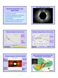
Corona at <strong>solar</strong> eclipse<br />
White light corona<br />
(LASCO C3 / SOHO, MPAe)<br />
�� Active regions<br />
(loops)<br />
�� Quiet Sun<br />
�� X-ray ray bright points<br />
�� Coronal holes<br />
�� Arcades<br />
Fe XII 195 Å<br />
(1.500.000 K)<br />
17 May - 8 June 1998<br />
1980<br />
1988<br />
Solar corona during eclipses<br />
1991<br />
1994<br />
Coronal structure: active region loops<br />
Coronal structure: streamers <strong>The</strong> <strong>solar</strong> wind<br />
TRACE, 1999<br />
A constant stream of particles flowing from the Sun’s<br />
corona, with a temperature of about a million degrees<br />
and with a velocity of about 450 km/s. <strong>The</strong> <strong>solar</strong> wind<br />
reaches out beyond Pluto's orbit, with the heliopause<br />
located roughly at<br />
100-120 100 120 AU<br />
5
Comets and the <strong>solar</strong> wind<br />
Comet<br />
NEAT<br />
(C/2002 V1)<br />
3-D structure of the Solar Wind:<br />
Variation over the Solar Cycle<br />
1st Orbit: 3/1992 - 11/1997<br />
declining / minimum phase<br />
Ulysses SWICS data<br />
2nd Orbit: 12/1997 - 2/2002<br />
rising / maximum phase<br />
Woch et al. GRL<br />
Parker’s theory of the <strong>solar</strong> wind<br />
�� Basic idea: dynamic equilibrium between hot corona<br />
and interstellar medium. Mass and momentum<br />
balance equations:<br />
d 2<br />
( ρr<br />
v)<br />
= 0<br />
dr<br />
dv 1 dP GM<br />
v = −<br />
2<br />
dr dr r<br />
��Parker’s Parker’s Eq. Eq.<br />
for <strong>solar</strong> wind speed (isothermal<br />
<strong>atmosphere</strong>)<br />
2<br />
1 dv 2 2 2c<br />
GM<br />
S<br />
( v − cS<br />
) = − 2<br />
v dr<br />
r r<br />
ρ<br />
Solar wind characteristics at 1AU<br />
Fast <strong>solar</strong> wind Slow <strong>solar</strong> wind<br />
�� speed > 400 km/s 2000 km/s<br />
�� Variable B, with B up to 100 nT (0.01G)<br />
�� Often very low density<br />
�� Sometimes up to 30% He<br />
�� Often associated with interplanetary shock waves<br />
�� Origin: CMEs<br />
Coronal Shape & Solar Wind:<br />
Ulysses Data & 3D-Heliosphere<br />
Activity minimum Activity maximum<br />
Parker’s <strong>solar</strong> wind solutions<br />
�� Parker found 4<br />
CHECK WHY ONLY ONE SOLN<br />
families of <strong>solar</strong> wind<br />
IS CORRECT!!!!!!!!!<br />
solutions<br />
�� 2 not supported by<br />
Obs. Obs.<br />
(supersonic at<br />
<strong>solar</strong> surface)<br />
�� 1 does not give<br />
sufficient pressure<br />
against the<br />
interstellar medium.<br />
�� Correct solution<br />
must be thick line in<br />
Fig.<br />
6
�� Speed of<br />
<strong>solar</strong> wind<br />
predicted by<br />
Parker’s<br />
model for<br />
different<br />
coronal<br />
temperatures<br />
(simple,<br />
isothermal<br />
case; no<br />
magnetic<br />
field)<br />
Solar wind speed<br />
Magnetic Field<br />
Correlation of field with brightness<br />
<strong>The</strong> Heliosphere<br />
Heliopause<br />
Heliotail<br />
Heliospheric<br />
shock<br />
Bowshock<br />
Interstellar<br />
medium<br />
<strong>The</strong> source of the Sun’s<br />
activity is the magnetic field<br />
Thomas Wiegelmann<br />
�� Heliosphere = region<br />
of space in which the<br />
<strong>solar</strong> wind and <strong>solar</strong><br />
magnetic field<br />
dominate over the<br />
instellar medium and<br />
the galactic magnetic<br />
field.<br />
�� Bowshock: Bowshock where the<br />
interstellar medium is<br />
slowed relative to the<br />
Sun.<br />
�� Heliospheric shock:<br />
where the <strong>solar</strong> wind<br />
is decelerated relative<br />
to Sun<br />
�� Heliopause: Heliopause boundary<br />
of the heliosphere<br />
�������� in order to<br />
understand the<br />
dynamics and<br />
activity of the Sun<br />
we need<br />
measurements and<br />
theory of its<br />
magnetic field<br />
Open and closed magnetic flux<br />
Closed flux: flux:<br />
slow<br />
<strong>solar</strong> wind<br />
Most of the <strong>solar</strong> flux<br />
returns to the <strong>solar</strong><br />
surface within a few<br />
R�� (closed closed flux) flux<br />
A small part of the<br />
total flux through the<br />
<strong>solar</strong> surface<br />
connects as open<br />
flux to interplanetary<br />
space<br />
Open flux: flux:<br />
fast <strong>solar</strong><br />
wind<br />
7
Measured<br />
Magnetic<br />
Field at<br />
Sun’s<br />
Surface<br />
Month long<br />
sequence of<br />
magnetograms<br />
(approx. one<br />
<strong>solar</strong> rotation)<br />
MDI/SOHO<br />
May 1998<br />
Example of proxies: Continuum vs. Gband<br />
Continuum G-band G band<br />
Hα and the chromospheric field<br />
�� Hα images of active<br />
regions show a<br />
structure similar to<br />
iron filing around a<br />
magnet. Do they<br />
(roughly) follow the<br />
field lines?<br />
�� Relatively horizontal<br />
field in<br />
chromosphere?<br />
chromosphere<br />
�� Note spiral structure<br />
around sunspot.<br />
Methods of magnetic field<br />
measurement<br />
�� Direct methods:<br />
�� Zeeman effect �� polarized radiation<br />
�� Hanle effect �� polarized radiation<br />
�� Gyroresonance �� radio spectra<br />
�� Indirect methods: Proxies<br />
�� Bright or dark features in photosphere (sunspots,<br />
G-band band bright points)<br />
�� Ca II H and K plage<br />
�� Fibrils seen in chromospheric lines, e.g. Hα H<br />
�� Coronal loops seen in EUV or X-radiation X radiation<br />
Ca II K as a magnetic field proxy<br />
�� Ca II H and K lines,<br />
the strongest lines<br />
in the visible <strong>solar</strong><br />
spectrum, show a<br />
strongly increasing<br />
brightness with<br />
non-spot non spot magnetic<br />
flux.<br />
�� <strong>The</strong> increase is<br />
slower than linear<br />
�� Magnetic regions<br />
(except sunspots)<br />
appear bright in Ca<br />
II: Ca plage and<br />
network regions<br />
Zeeman diagnostics<br />
�� Direct detection of magnetic field by<br />
observation of magnetically induced splitting<br />
and polarisation of spectral lines<br />
�� Important: Zeeman effect changes not just<br />
the spectral shape of a spectral line (often<br />
subtle and difficult to measure), but also<br />
introduces a unique polarisation signature<br />
��Measurement Measurement of polarization is central to<br />
measuring <strong>solar</strong> magnetic fields.<br />
8
Polarized radiation<br />
�� Polarized<br />
radiation is<br />
described by<br />
the 4 Stokes<br />
parameters: I, Q, U and V<br />
�� I = total intensity = Ilin lin(0 (0o ) + Ilin lin(90 (90o ) = Ilin lin(45 (45o ) + Ilin lin(135 (135o ) =<br />
Icirc circ(right (right) ) + Icirc circ(left) (left)<br />
�� Q = Ilin lin(0 (0o ) - Ilin lin(90 (90o )<br />
�� U = Ilin lin(45 (45o ) - Ilin lin(135 (135o )<br />
�� V = Icirc circ(right) (right) - Icirc circ(left) (left)<br />
�� Note: Stokes parameters are sums and differences of<br />
intensities, i.e. they are directly measurable<br />
Splitting patterns of lines<br />
�� Depending on g of the<br />
upper and lower levels,<br />
the spectral line shows<br />
different splitting<br />
patterns<br />
�� Positive: π components:<br />
∆M=0 =0<br />
�� Negative: σ<br />
components: ∆M=±1<br />
�� Top left: normal<br />
Zeeman effect (rare)<br />
�� Rest: anomalous<br />
Zeeman effect (usual)<br />
Effect of changing field strength<br />
Formula for Zeeman splitting (for ( for B in G, λ in Å): ):<br />
∆λ H = 4.67 10 -13 13<br />
geff effBλ2 [Å] ]<br />
geff=effective eff=effective<br />
Lande factor of line<br />
For large B: : ∆λ H = ∆λ between σ-component component peaks<br />
I<br />
B=1600 G<br />
B=200 G<br />
V<br />
Zeeman splitting of atomic levels<br />
�� In the presence of a B-<br />
field a level with total<br />
angular moment J will<br />
split into 2J+1 +1 sublevels<br />
with different M.<br />
�� E J,M = E J+µ 0 gM JB<br />
�� Transitions are allowed<br />
between levels with<br />
∆J J = 0,±1 0, 1 & ∆M M = 0 (π), ( ,<br />
±1 1 (σ ( b, , σr) �� Splitting is determined<br />
by Lande factor g :<br />
g(J,L,S J,L,S) ) = 1+(J(J+1)+ 1+( +1)+<br />
S(S+1) +1)-L(L+1))/2 +1))/2J(J+1) +1)<br />
Polarization and Zeeman effect<br />
Dependence on B, γ, & φ<br />
�� I ~ κσ(1+ (1+cos cos2γ)/4 )/4 + κπ sin 2γ/2 /2<br />
�� Q ~ B 2 sin 2γ cos 2φ<br />
�� U ~ B 2 sin 2γ sin 2φ 2<br />
�� V ~ B cos γ<br />
�� Q, U: U:<br />
transverse<br />
component of B<br />
�� V: : longitudinal<br />
component of B<br />
Juanma Borrero<br />
9
Zeeman polarimetry<br />
�� Most used remote sensing of astrophysical<br />
(and certainly <strong>solar</strong>) magnetic fields<br />
�� Effective measurement of field strength if<br />
Zeeman splitting is comparable to Doppler<br />
width or more: B > 200 00 G … 1000 G<br />
(depending on spectral line) �� works best in<br />
photosphere<br />
�� Splitting scales with λ �� works best in IR<br />
�� Sensitive to cancellation of opposite magnetic<br />
polarities �� needs high spatial resolution<br />
Cancellation of magnetic polarity<br />
= positive polarity<br />
magnetic field<br />
= negative polarity<br />
magnetic field<br />
Spatial resolution<br />
element<br />
What does a<br />
magnetogram show?<br />
�� Plotted at left:<br />
�� Top: Stokes I, Q and V along<br />
a spectrograph slit<br />
�� Middle: Sample Stokes Q<br />
profile<br />
�� Bottom: Sample Stokes V<br />
profile<br />
�� Red bars: example of a<br />
spectral range used to make<br />
a magnetogram. magnetogram.<br />
Generally<br />
only Stokes V is used<br />
(simplest to measure), gives<br />
longitudinal component of B.<br />
Effect of wavelength of spectral line<br />
I<br />
V<br />
Q U<br />
�� Magnetograph:<br />
Instrument that<br />
makes maps of (net<br />
circular) polarization<br />
in wing of Zeeman<br />
sensitive line.<br />
�� Example of<br />
magnetogram<br />
obtained by MDI<br />
�� Conversion of<br />
polarization into<br />
magnetic field<br />
requires a careful<br />
calibration.<br />
Magnetograms<br />
Synoptic charts<br />
Fe I 1564.8 630.2 nm<br />
Synoptic maps approximate the radial magnetic flux observed<br />
near the central meridian over a period of 27.27 days (= 1<br />
Carrington rotation)<br />
10
Polarized radiative transfer<br />
�� Complication: RTE required for 4 Stokes<br />
parameters: Written as differential equation<br />
for Stokes vector Iν= (Iν ,Q ν ,U ν ,V ν)<br />
�� Eq. Eq.<br />
in plane parallel <strong>atmosphere</strong> for a<br />
spectral line (Unno ( Unno-Rachkowsky<br />
Rachkowsky equations):<br />
µ dIν /dτc = ΩνIν – Sν �� Ων = absorption matrix (basically ratio of line<br />
to continuum absorption coefficient), Sν= =<br />
source function vector, τc = continuum optical<br />
depth.<br />
Polarized radiative transfer III<br />
�� <strong>The</strong> Zeeman effect only enters through Ων �� Ων contains besides absorption due to<br />
Zeeman-split Zeeman split line (ηI I , ηQ Q , ηU U , ηV V ) also<br />
magnetooptical effects, such as Faraday<br />
rotation (ρQ Q , ρU U , ρV V ) : rotation of plane of<br />
polarization when light passes through B.<br />
�� Ων = Ων(γ, , φ, , B) B)<br />
, i.e. Ων depends on the full<br />
magnetic vector (in addition to the usual<br />
quantities that the absorption coefficient<br />
depends on)<br />
Solution of Unno Eqs<br />
�� General solution best done numerically (even formal<br />
solution is non-trivial: non trivial: exponent of matrix Ων )<br />
�� Simple analytical solutions exist for a Milne- Milne<br />
Eddington <strong>atmosphere</strong> (i.e. for Ων independent of τν and Sν depending only linearly on τν). ). Particularly<br />
simple if we neglect magneto-optical magneto optical effects<br />
�� I(µ) I( ) = β µ (1+η (1+ I)/ )/∆<br />
�� P(µ)= P( )= β µ ηP /∆, where P = Q, U, or V<br />
�� ∆ = (1+η (1+ I ) 2 - ηQ 2 - ηU 2 - η 2<br />
V<br />
takes care of line saturation<br />
�� β is derivative of <strong>Planck</strong> function with respect to τν .<br />
Polarized radiative transfer II<br />
<strong>The</strong> absorption matrix<br />
⎛1+<br />
ηI<br />
ηQ<br />
ηU<br />
ηV<br />
⎞<br />
⎜<br />
⎟<br />
⎜ ηQ<br />
1+<br />
ηI<br />
− ρV<br />
ρU<br />
⎟<br />
Ων<br />
= ⎜ η<br />
⎟<br />
U ρV<br />
1+<br />
ηI<br />
ρQ<br />
⎜<br />
⎟<br />
⎜<br />
⎟<br />
⎝ ηV<br />
− ρU<br />
− ρQ<br />
1+<br />
ηI<br />
⎠<br />
SAY MORE ABOUT MATRIX ELEMENTS!!!!!!<br />
SHOW HOW ZEEMAN EFFECT ENTERS<br />
INTO THEM, ETC.!!!!!<br />
LTE<br />
�� In LTE the Unno-Rachkowsky<br />
Unno Rachkowsky equations simplify<br />
since<br />
Sν= = (B ( ν , 0, 0, 0)<br />
Here Bν = <strong>Planck</strong> function<br />
�� Also, Ων is simplified. <strong>The</strong> ηI I , ηQ Q , ηU U , ηV V and ρQ Q , ρU U ,<br />
ρV V values only require application of Saha- Saha<br />
Boltzmann equations (similar situation as for LTE in<br />
case of normal radiative transfer). Each of these<br />
quantities is, of course, frequency dependent.<br />
Basics: magnetic pressure<br />
�� Magnetic field exerts a pressure. Pressure balance between<br />
two components of the <strong>atmosphere</strong>, 1 and 2 (Gauss units):<br />
2<br />
2<br />
B1<br />
B2<br />
+<br />
P1<br />
= P2<br />
+<br />
8π<br />
8π<br />
�� If, e.g. B 2 = 0, then P1 < P2 and it follows:<br />
��Magnetic Magnetic features are evacuated compared to surroundings.<br />
�� If B 2 = 0 and T1 = T 2, , then also ρ1 < ρ2 , so that the magnetic<br />
features are buoyant compared to the surrounding gas.<br />
�� In the convection zone this buoyancy means that rising field<br />
bundles (flux tubes) keep rising (unless stopped by other<br />
forces, e.g. curvature forces.<br />
11
Basics: plasma β<br />
�� Plasma β describes the ratio of thermal to magnetic<br />
energy density:<br />
8πP<br />
β = 2<br />
B<br />
�� β < 1 �� Magnetic field dominates and dictates the<br />
dynamics of the gas<br />
�� β >1 �� <strong>The</strong>rmal energy, i.e. gas dominates & forces<br />
the field to follow<br />
�� β changes with r/R ��<br />
�� β >1 in convection zone<br />
�� β
<strong>The</strong> photospheric field<br />
Sunspot<br />
umbra<br />
penumbra<br />
quiet<br />
Sun<br />
plage<br />
Sunspots, some properties<br />
�� Field strength: strength:<br />
Peak values<br />
2000-3500 2000 3500 G<br />
�� Brightness: Brightness:<br />
umbra: 20% of<br />
quiet Sun, penumbra: 75%<br />
�� Sizes: Sizes:<br />
Log-normal Log normal size<br />
distribution. Overlap with<br />
pores (log-normal (log normal =<br />
Gaussian on a logarithmic<br />
scale)<br />
�� Lifetimes: Lifetimes:<br />
T between hours &<br />
months: Gnevyshev-<br />
Gnevyshev<br />
Waldmeier rule: Amax max ~ T,<br />
where Amax max = max spot area.<br />
Why are sunspots dark? II<br />
�� Where does the energy blocked by sunspots go?<br />
�� Spruit (1982) showed: both heat capacity and<br />
thermal conductivity of CZ gas is very large<br />
��High High thermal conductivity: blocked heat is<br />
redistributed throughout CZ (no bright rings around<br />
sunspots)<br />
High heat capacity: the additional heat does not lead<br />
to a measurable increase in temperature<br />
�� In addition: time scale for thermal relaxation of the<br />
CZ is long, 10 5 years: excess energy is released<br />
almost imperceptibly.<br />
Sunspots<br />
Umbra Penumbra Granule<br />
Teff eff ≈ 4500 K<br />
Teff eff ≈ 5500 K<br />
Teff eff ≈ 5800 K<br />
Why are sunspots dark?<br />
�� Basically the strong nearlly vertical magnetic field, not<br />
allowing motions across the field lines, quenches convection<br />
inside the spot.<br />
�� Since convection is the main source of energy transport just<br />
below the surface, less energy reaches the surface through<br />
the spot �� dark<br />
Magnetic structure of<br />
sunspots<br />
�� Peak field strength ≈ 2000 –<br />
3500 G (usually in darkest,<br />
central part of umbra)<br />
�� B drops steadily towards<br />
boundary, B(Rspot) spot)<br />
≈ 1000 G<br />
�� At centre, field is vertical,<br />
becoming almost horizontal<br />
near Rspot spot .<br />
�� Regular spots have a field<br />
structure similar to a buried<br />
dipole<br />
1
Magnetic<br />
structure of<br />
sunspots II<br />
Azimuthal averages of<br />
the various magnetic<br />
field components in a<br />
sample of regular (near-<br />
circular) medium-sized<br />
medium sized<br />
sunspots.<br />
Sunspot fine structure<br />
Sunspots<br />
Penumbral filaments<br />
(bright and dark)<br />
Penumbral grain (seen<br />
to move inward)<br />
Light bridge<br />
Umbral dot<br />
TiO Zakharov 2004<br />
Magnetic structure of sunspots<br />
Schlichenmaier et al.<br />
1998, 1999, 2002<br />
�� Regular on large scales (≈ ( dipole, B max ≈ 2500 G, for simple<br />
spots)<br />
�� Extremely complex on small scales (penumbra, subsurface)<br />
V. Zakharov<br />
Highest resolution<br />
Scharmer et al. 2002<br />
Umbral dots seen in TiO<br />
2
Magnetic structure of sunspots<br />
X?<br />
Sunspots span too many spatial and temporal scales<br />
to be successfully simulated from first principles.<br />
�� Horizontal<br />
outflow of<br />
matter.<br />
�� Thought to be<br />
driven by a<br />
siphon flow<br />
mechanism<br />
�� NEED NEW<br />
SLIDE !!!!!!!<br />
Evershed effect: illustration<br />
<strong>The</strong> Wilson effect<br />
�� Near the <strong>solar</strong><br />
limb the umbra<br />
and centre-side<br />
centre side<br />
penumbra<br />
disappear<br />
��We We see 400-800 400 800<br />
km deeper into<br />
sunspots than in<br />
photosphere<br />
�� Correct<br />
interpretation<br />
by Wilson (18 th<br />
Other interpretation by e.g. W. Herschell: Herschell:<br />
photosphere is a layer of hot clouds<br />
century).<br />
through which we see deeper, cool layers:<br />
the true, populated surface of the Sun.<br />
Evershed effect<br />
In photospheric layers penumbra shows nearly horizontal<br />
outward motion, visible as oppositely directed Doppler shifts<br />
(umbra remains at rest). In chromosphere: chromosphere:<br />
inward directed flow<br />
Brightness Doppler shift<br />
Siphon flow model of Evershed effect<br />
�� Proposed by Meyer & Schmidt (1968).<br />
�� If there is an imbalance in the field strength of the<br />
two footpoints of a loop, then gas will flow from the<br />
footpoint with<br />
lower B to that<br />
with higher B.<br />
�� Supersonic<br />
flows are<br />
possible.<br />
B 1<br />
< B 2<br />
Sunspot Wilson depression<br />
Map of Wilson depression<br />
(determined from T & B measurements and assumption<br />
that sunspot magnetic field is close to potential)<br />
Shibu Mathew<br />
3
What causes the Wilson depression?<br />
�� B square/8 pi means gas pressure lower in<br />
spot than outside i.e. density also lower, i.e.<br />
fewer atoms to absorb, i.e. opacity also lower<br />
�� we see deeper into spot<br />
Surprisingly constant field strength<br />
Magn. Magn.<br />
elements Pores Sunspots<br />
Temperature stratifications of quiet<br />
Sun, sunspot, plage<br />
�� Dashed line: Quiet Sun<br />
<strong>atmosphere</strong><br />
�� Solid line: sunspot<br />
<strong>atmosphere</strong><br />
�� Dot-dashed Dot dashed line: active<br />
region plage <strong>atmosphere</strong><br />
�� Plage is hottest<br />
everywhere in<br />
<strong>atmosphere</strong><br />
�� Sunspot coldest in<br />
photosphere, but gets<br />
hotter in chromosphere<br />
Magnetic elements<br />
�� Most of the magnetic flux on the <strong>solar</strong> surface<br />
occurs outside sunspots and pores (=smaller<br />
dark magnetic structures).<br />
�� <strong>The</strong>se most common magnetic features,<br />
called magnetic elements, are small<br />
(diameters partly below spatial resolution of<br />
100 km), bright and concentrated in network<br />
and facular regions.<br />
�� Magnetic elements are usually described by<br />
thin magnetic flux tubes (i.e. bundles of nearly<br />
parallel field lines).<br />
Temperature contrast vs. size<br />
Magn. Magn.<br />
elements Pores Sunspots<br />
Increased<br />
contrast of<br />
magnetic<br />
elements in<br />
higher layers<br />
4
Why are magnetic elements bright?<br />
`Hot wall´ radiation<br />
•Quenching Quenching of convection<br />
•Partial Partial evacuation<br />
→ enhanced transparency<br />
→ heating by `hot walls´ walls<br />
→ local local flux flux excess excess<br />
•Inflow Inflow of radiation wins<br />
because the flux tubes are<br />
narrow (diameter ~ Wilson<br />
depression).<br />
•High High heat conductivity<br />
→ flux disturbance partly<br />
propagates into the<br />
deep convection zone<br />
→ Kelvin-Helmholtz<br />
Kelvin Helmholtz time<br />
Flux tube brightening near limb<br />
�� <strong>The</strong> flux tubes expand with height (pressure balance<br />
�� <strong>The</strong>y appear brightest when hot walls are well seen, i.e. near limb limb<br />
(closer<br />
to limb for larger tubes<br />
B z<br />
Details of<br />
thin<br />
magnetic<br />
flux<br />
sheet<br />
T<br />
Steiner et al. 1994<br />
Horizontal cuts near surface level Vögler et al. 2005<br />
v z<br />
I C<br />
Why are<br />
faculae<br />
best<br />
seen<br />
near<br />
limb?<br />
<strong>The</strong> Sun in<br />
White Light,<br />
with limb<br />
darkening<br />
removed<br />
MDI on SOHO<br />
Bz (Z=0)<br />
>500G<br />
>1000G<br />
>1500G<br />
. Mixed<br />
3-D D compressible<br />
radiation-MHD<br />
radiation MHD<br />
simulations<br />
Plage: BZ(t=0) (t=0) = 200 G<br />
Grid Size: 288 x 288 x 100<br />
Vertical extent: 1.4 Mm<br />
Horizontal extent: 6 Mm<br />
Alexander Vögler et al.<br />
6<br />
Mm<br />
3-D Radiation-MHD Simulations<br />
vz z<br />
(Z=0)<br />
Ic (Z=0)<br />
Alexander Vögler, Robert Cameron, Manfred Schüssler<br />
Mixed polarity simulations: diffusion & cancellation of opposite opposite<br />
polarities (20 km resolution): =200G. >=200G.<br />
. B z Bz < 200 G<br />
6000 km<br />
1
Simulations require computers...<br />
G-band:<br />
Simulation vs. Observation<br />
Simulation (20 km resolution)<br />
Schüssler et al. 2003<br />
Shelyag et al. 2004<br />
Producing Stokes<br />
V asymmetry<br />
�� Consider 2-layered 2 layered<br />
<strong>atmosphere</strong>:<br />
�� Bottom layer a: : v but<br />
no B<br />
�� Top layer b: : B but no v<br />
�� Note the importance<br />
of line saturation for<br />
producing asymmetric<br />
V profile.<br />
Observation (100 km resol.)<br />
(SST, La Palma)<br />
Scharmer et al. 2002<br />
d<br />
c<br />
b<br />
a<br />
G-band Spectrum Synthesis<br />
G-Band (Fraunhofer): spectral range: 4295-4315 Å<br />
contains many temperature-sensitive molecular lines (CH)<br />
For comparison with observations, we define as G-band<br />
intensity the integral of the spectrum obtained from the<br />
simulation data:<br />
4315 A<br />
IG<br />
= ∫ I ( λ ) dλ<br />
Shelyag et al. 2004<br />
�� Stokes V profiles<br />
observed in quiet<br />
Sun and in active<br />
region plage are<br />
asymmetric:<br />
typically blue wing<br />
has larger area ‘A’<br />
and amplitude ‘a’<br />
than red wing<br />
4295 A<br />
Stokes V asymmetry<br />
Flux Tubes, Canopies, Loops and<br />
Funnels<br />
1
Measurement of B at coronal base<br />
�� Previously: Magnetic<br />
vector only known at <strong>solar</strong><br />
surface. However, magnetic<br />
field has main effect in corona.<br />
Exception: radio observations<br />
give |B| but low resolution.<br />
�� Now: Direct measurement of<br />
full magnetic vector at base of<br />
corona & in cool loops<br />
possible<br />
�� Measurement using He I<br />
10830 Å (TIP, VTT, Tenerife)<br />
& simple inversion code<br />
Solanki et al. 2003, Lagg et al. 2004<br />
Magnetic field extrapolations: Force<br />
free and potential fields<br />
�� General problem in <strong>solar</strong> physics: Magnetic field is<br />
measured mainly in the photosphere, but it makes<br />
the music mainly in the corona.<br />
��Either Either improve coronal field measurements or<br />
extrapolate from photospheric measurements into<br />
the corona.<br />
�� If β
Prominence<br />
models<br />
Kippenhahn-Schl<br />
Kippenhahn Schlüter ter<br />
(below), Kuperus-Raadu<br />
Kuperus Raadu<br />
(below right) and flux tube<br />
(right)<br />
Solar current sheet at activity minimum<br />
�� At activity minimum<br />
<strong>solar</strong> magnetic field<br />
is like a dipole,<br />
whose field lines are<br />
stretched out by the<br />
<strong>solar</strong> wind.<br />
�� Field lines with<br />
opposite polarity lie<br />
close to each other<br />
near equator:<br />
euatorial current<br />
sheet.<br />
�� If dipole axis inclined<br />
to ecliptic: magnetic<br />
polarity at Earth<br />
changes over <strong>solar</strong><br />
rotation.<br />
Large scale magnetic structure of the<br />
quiet Sun<br />
�� At large scales<br />
dipolar<br />
component of the<br />
magnetic field<br />
survives, since<br />
multipoles ��<br />
B~r -n-1 , where<br />
n=2 for dipole,<br />
n=3 for<br />
quadrupole, quadrupole,<br />
etc.<br />
�� Closer to sun<br />
ever higher order<br />
multipoles are<br />
important<br />
Heliospheric current sheet and Parker<br />
spiral<br />
�� Since <strong>solar</strong> wind expands radially beyond the Alfven radius<br />
(where the energy density in the wind exceeds that in the<br />
magnetic field) and the Sun rotates (i.e. the footpoints of the<br />
field), the structure of the field (carried out by the wind, but<br />
anchored on rotating surface) shows a spiral structure.<br />
2