The Laplace Transform
The Laplace Transform
The Laplace Transform

You also want an ePaper? Increase the reach of your titles
YUMPU automatically turns print PDFs into web optimized ePapers that Google loves.
<strong>The</strong> <strong>Laplace</strong> <strong>Transform</strong><br />
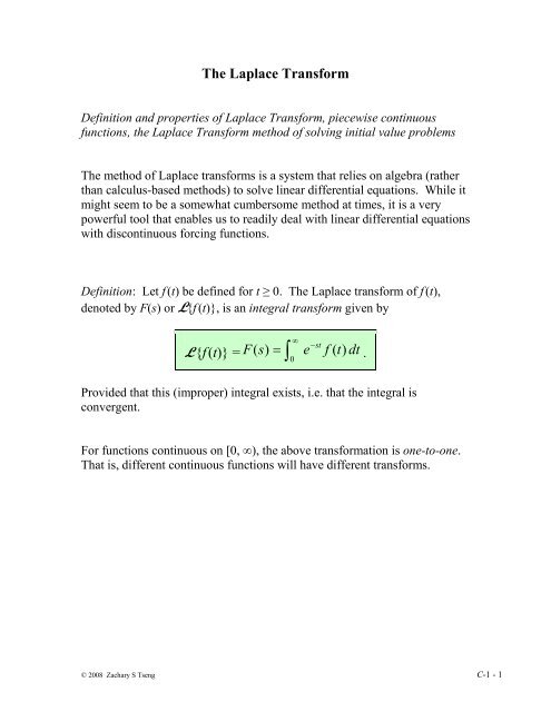
Definition and properties of <strong>Laplace</strong> <strong>Transform</strong>, piecewise continuous<br />
functions, the <strong>Laplace</strong> <strong>Transform</strong> method of solving initial value problems<br />
<strong>The</strong> method of <strong>Laplace</strong> transforms is a system that relies on algebra (rather<br />
than calculus-based methods) to solve linear differential equations. While it<br />
might seem to be a somewhat cumbersome method at times, it is a very<br />
powerful tool that enables us to readily deal with linear differential equations<br />
with discontinuous forcing functions.<br />
Definition: Let f (t) be defined for t ≥ 0. <strong>The</strong> <strong>Laplace</strong> transform of f (t),<br />
denoted by F(s) or L{f (t)}, is an integral transform given by<br />
L {f (t)} = ∫ ∞<br />
−st<br />
F(<br />
s)<br />
e f ( t)<br />
dt .<br />
= 0<br />
Provided that this (improper) integral exists, i.e. that the integral is<br />
convergent.<br />
For functions continuous on [0, ∞), the above transformation is one-to-one.<br />
That is, different continuous functions will have different transforms.<br />
© 2008 Zachary S Tseng C-1 - 1
Example: Let f (t) = 1, then<br />
L{f (t)} =<br />
1<br />
F(<br />
s)<br />
= , s > 0.<br />
s<br />
∞<br />
∞<br />
−st<br />
−st<br />
−st<br />
∞<br />
∫ e f ( t)<br />
dt = ∫ e dt = e<br />
0<br />
0<br />
0<br />
© 2008 Zachary S Tseng C-1 - 2<br />
−1<br />
s<br />
<strong>The</strong> integral is divergent whenever s ≤ 0. However, when s > 0, it<br />
converges to<br />
−<br />
s<br />
−1<br />
1<br />
( 0 − e ) = ( −1)<br />
= = F(<br />
s)<br />
1 0<br />
s<br />
1<br />
Example: Let f (t) = t, then F ( s)<br />
= 2 , s > 0.<br />
s<br />
[This is left to you as an exercise.]<br />
Example: Let f (t) = e at , then<br />
L{f (t)} =<br />
s<br />
.<br />
F s =<br />
s − a<br />
1<br />
( ) , s > a.<br />
1 t<br />
a − s<br />
∞<br />
∞<br />
−st<br />
at<br />
( a−s<br />
) t<br />
( a−s<br />
)<br />
∞<br />
∫ e e dt = ∫ e dt = e<br />
0<br />
0<br />
0<br />
<strong>The</strong> integral is divergent whenever s ≤ a. However, when s > a, it<br />
converges to<br />
1 1<br />
( 0 − e ) = ( −1)<br />
= = F(<br />
s)<br />
1 0<br />
a − s<br />
a − s<br />
s − a<br />
.
Definition: A function f (t) is called piecewise continuous if it only has<br />
finitely many (or none whatsoever – a continuous function is considered to<br />
be “piecewise continuous”!) discontinuities on any interval [a, b], and that<br />
both one-sided limits exist as t approaches each of those discontinuity from<br />
within the interval. <strong>The</strong> last part of the definition means that f could have<br />
removable and/or jump discontinuities only; it cannot have any infinity<br />
discontinuity.<br />
<strong>The</strong>orem: Suppose that<br />
1. f is piecewise continuous on the interval 0 ≤ t ≤ A for any A > 0.<br />
2. │f (t)│ ≤ K e at when t ≥ M, for any real constant a, and any positive<br />
constants K and M. (This means that f is “of exponential order”, i.e.<br />
its rate of growth is no faster than that of exponential functions.)<br />
<strong>The</strong>n the <strong>Laplace</strong> transform, F(s) = L{f (t)}, exists for s > a.<br />
Note: <strong>The</strong> above theorem gives a sufficient condition for the existence of<br />
<strong>Laplace</strong> transforms. It is not a necessary condition. A function does not<br />
need to satisfy the two conditions in order to have a <strong>Laplace</strong> transform.<br />
Examples of such functions that nevertheless have <strong>Laplace</strong> transforms are<br />
logarithmic functions and the unit impulse function.<br />
© 2008 Zachary S Tseng C-1 - 3
Some properties of the <strong>Laplace</strong> <strong>Transform</strong><br />
1. L {0} = 0<br />
2. L {f (t) ± g(t)} = L {f (t)} ± L {g(t)}<br />
3. L {c f (t)} = c L {f (t)}, for any constant c.<br />
Properties 2 and 3 together means that the <strong>Laplace</strong> transform is linear.<br />
4. [<strong>The</strong> derivative of <strong>Laplace</strong> transforms]<br />
L {(−t)f (t)} = F ′(s) or, equivalently L {t f (t)} = −F ′(s)<br />
d 1 − 2 2<br />
− = − =<br />
ds s s s<br />
Example: L {t 2 } = − (L {t})′ = 2 3 3<br />
In general, the derivatives of <strong>Laplace</strong> transforms satisfy<br />
L {(−t) n f (t)} = F (n) (s) or, equivalently L {t n f (t)} = (−1) n F (n) (s)<br />
Warning: <strong>The</strong> <strong>Laplace</strong> transform, while a linear operation, is not<br />
multiplicative. That is, in general<br />
L {f (t) g(t)} ≠ L {f (t)} L {g(t)}.<br />
Exercise: (a) Use property 4 above, and the fact that L { e at } =<br />
1<br />
( s − a)<br />
to deduce that L {t e at } = 2 . (b) What will L {t 2 e at } be?<br />
1<br />
,<br />
s − a<br />
© 2008 Zachary S Tseng C-1 - 4
Exercises C-1.1:<br />
1 – 5 Use the (integral transformation) definition of the <strong>Laplace</strong> transform<br />
to find the <strong>Laplace</strong> transform of each function below.<br />
1. t 2 2. t e 6t<br />
3. cos 3t 4. e −t sin 2t<br />
5.* e iαt , where i and α are constants, i = −1<br />
.<br />
6 – 8 Each function F(s) below is defined by a definite integral. Without<br />
integrating, find an explicit expression for each F(s).<br />
[Hint: each expression is the <strong>Laplace</strong> transform of a certain function. Use<br />
your knowledge of <strong>Laplace</strong> <strong>Transform</strong>ation, or with the help of a table of<br />
common <strong>Laplace</strong> transforms to find the answer.]<br />
6. ∫ ∞<br />
−(<br />
s+<br />
7)<br />
t<br />
e dt 7. ∫ ∞<br />
2 −(<br />
s−3)<br />
t<br />
t e dt<br />
0<br />
8. ∫ ∞<br />
0<br />
−<br />
4e sin 6t<br />
dt<br />
st<br />
0<br />
Answers C-1.1:<br />
2<br />
1. 3<br />
s 2. 1<br />
2<br />
( s − 6)<br />
s<br />
2<br />
3. 2 4. 2<br />
s + 9<br />
s + 2s<br />
+ 5<br />
s α<br />
5. + i<br />
2 2 2 2<br />
s + α s + α<br />
Note: Since the Euler’s formula says that e iαt = cos αt + i sin αt, therefore,<br />
L{e iαt } = L{cos αt + i sin αt}. That is, the real part of its <strong>Laplace</strong> transform<br />
corresponds to that of cos αt, the imaginary part corresponds to that of sin αt.<br />
(Check it for yourself!)<br />
1<br />
2<br />
24<br />
6.<br />
7. 3<br />
8. 2<br />
s + 7<br />
( s − 3)<br />
s<br />
+ 36<br />
© 2008 Zachary S Tseng C-1 - 5
Solution of Initial Value Problems<br />
We now shall meet “the new System”: how the <strong>Laplace</strong> transforms can be<br />
used to solve linear differential equations algebraically.<br />
<strong>The</strong>orem: [<strong>Laplace</strong> transform of derivatives] Suppose f is of exponential<br />
order, and that f is continuous and f ′ is piecewise continuous on any interval<br />
0 ≤ t ≤ A. <strong>The</strong>n<br />
L {f ′(t)} = s L {f (t)} − f (0)<br />
Applying the theorem multiple times yields:<br />
L {f ″(t)} = s 2 L {f (t)} − s f (0) − f ′(0),<br />
L {f ″′(t)} = s 3 L {f (t)} − s 2 f (0) − s f ′(0) − f ″(0),<br />
:<br />
:<br />
L {f (n) (t)} = s n L {f (t)} − s n − 1 f (0) − s n − 2 f ′(0) − …<br />
− s 2 f (n −3) (0) − s f (n −2) (0) − f (n −1) (0).<br />
This is an extremely useful aspect of the <strong>Laplace</strong> transform: that it changes<br />
differentiation with respect to t into multiplication by s (and, as seen a little<br />
earlier, differentiation with respect to s into multiplication by −t, on the other<br />
hand). Equally importantly, it says that the <strong>Laplace</strong> transform, when applied<br />
to a differential equation, would change derivatives into algebraic<br />
expressions in terms of s and (the transform of) the dependent variable itself.<br />
Thus, it can transform a differential equation into an algebraic equation.<br />
We are now ready to see how the <strong>Laplace</strong> transform can be used to solve<br />
differentiation equations.<br />
© 2008 Zachary S Tseng C-1 - 6
Solving initial value problems using the method of<br />
<strong>Laplace</strong> transforms<br />
To solve a linear differential equation using <strong>Laplace</strong> transforms, there are<br />
only 3 basic steps:<br />
1. Take the <strong>Laplace</strong> transforms of both sides of an equation.<br />
2. Simplify algebraically the result to solve for L{y} = Y(s) in terms<br />
of s.<br />
3. Find the inverse transform of Y(s). (Or, rather, find a function y(t)<br />
whose <strong>Laplace</strong> transform matches the expression of Y(s).) This<br />
inverse transform, y(t), is the solution of the given differential<br />
equation.<br />
<strong>The</strong> nice thing is that the same 3-step procedure works whether or not the<br />
differential equation is homogeneous or nonhomogeneous. <strong>The</strong> first two<br />
steps in the procedure are rather mechanical. <strong>The</strong> last step is the heart of the<br />
process, and it will take some practice. Let’s get started.<br />
© 2008 Zachary S Tseng C-1 - 7
© 2008 Zachary S Tseng C-1 - 8
Example: y″ − 6y′ + 5y = 0, y(0) = 1, y′(0) = −3<br />
[Step 1] <strong>Transform</strong> both sides<br />
L{y″ − 6y′ + 5y} = L{0}<br />
(s 2 L{y} − s y(0) − y′(0)) − 6(sL{y} − y(0)) + 5L{y} = 0<br />
[Step 2] Simplify to find Y(s) = L{y}<br />
(s 2 L{y} − s −(−3)) − 6(s L{y} − 1) + 5L{y} = 0<br />
(s 2 − 6 s + 5) L{y} − s + 9 = 0<br />
(s 2 − 6 s + 5) L{y} = s − 9<br />
L{y} =<br />
s<br />
2<br />
s − 9<br />
− 6s<br />
+ 5<br />
[Step 3] Find the inverse transform y(t)<br />
Use partial fractions to simplify,<br />
L{y} =<br />
s<br />
2<br />
s<br />
2<br />
s − 9 a b<br />
= +<br />
− 6s<br />
+ 5 s −1<br />
s − 5<br />
s − 9 a(<br />
s − 5)<br />
b(<br />
s −1)<br />
=<br />
+<br />
− 6s<br />
+ 5 ( s −1)(<br />
s − 5)<br />
( s − 5)(<br />
s −1)<br />
s −<br />
9 = a(<br />
s − 5)<br />
+ b(<br />
s −1)<br />
= ( a + b)<br />
s + ( −5a<br />
− b)<br />
© 2008 Zachary S Tseng C-1 - 9
Equating the corresponding coefficients:<br />
Hence,<br />
1 = a + b a = 2<br />
−9 = −5a − b b = −1<br />
L{y} =<br />
s<br />
2<br />
s − 9 2 1<br />
= − .<br />
− 6s<br />
+ 5 s −1<br />
s − 5<br />
<strong>The</strong> last expression corresponds to the <strong>Laplace</strong> transform of<br />
2e t − e 5t . <strong>The</strong>refore, it must be that<br />
y(t) = 2e t − e 5t .<br />
Many of the observant students no doubt have noticed an interesting aspect<br />
(out of many) of the method of <strong>Laplace</strong> transform: that it finds the particular<br />
solution of an initial value problem directly, without solving for the general<br />
solution first. Indeed, it usually takes more effort to find the general solution<br />
of an equation than it takes to find a particular solution!<br />
<strong>The</strong> <strong>Laplace</strong> <strong>Transform</strong> method can be used to solve linear differential<br />
equations of any order, rather than just second order equations as in the<br />
previous example. <strong>The</strong> method will also solve a nonhomogeneous linear<br />
differential equation directly, using the exact same three basic steps, without<br />
having to separately solve for the complementary and particular solutions.<br />
<strong>The</strong>se points are illustrated in the next two examples.<br />
© 2008 Zachary S Tseng C-1 - 10
Example: y′ + 2y = 4t e −2t , y(0) = −3.<br />
[Step 1] <strong>Transform</strong> both sides<br />
L{y′ + 2y} = L{4t e −2t }<br />
(sL{y} − y(0)) + 2L{y} = L{4t e −2t 4<br />
} = 2<br />
( s + 2)<br />
[Step 2] Simplify to find Y(s) = L{y}<br />
4<br />
(sL{y} − (−3)) + 2L{y} = 2<br />
( s + 2)<br />
4<br />
(s + 2) L{y} + 3 = 2<br />
( s + 2)<br />
4<br />
(s + 2) L{y} = 2 − 3<br />
( s + 2)<br />
2<br />
2<br />
4 3 4 − 3(<br />
s + 2)<br />
− 3s<br />
−12s<br />
− 8<br />
L{y} = − =<br />
=<br />
3<br />
3<br />
3<br />
( s + 2)<br />
s + 2 ( s + 2)<br />
( s + 2)<br />
[Step 3] Find the inverse transform y(t)<br />
By partial fractions,<br />
2<br />
− 3s<br />
−12s<br />
− 8 a<br />
L{y} =<br />
= 3<br />
( s + 2)<br />
( s + 2)<br />
b<br />
+<br />
( s + 2)<br />
© 2008 Zachary S Tseng C-1 - 11<br />
3<br />
2<br />
c<br />
+<br />
s + 2<br />
.
2<br />
− 3s<br />
−12s<br />
− 8 a<br />
= 3<br />
( s + 2)<br />
( s + 2)<br />
2<br />
a + bs + 2b<br />
+ cs + 4cs<br />
+ 4c<br />
cs<br />
=<br />
=<br />
3<br />
( s + 2)<br />
3<br />
b(<br />
s + 2)<br />
c(<br />
s + 2)<br />
+ + 3<br />
3<br />
( s + 2)<br />
( s + 2)<br />
© 2008 Zachary S Tseng C-1 - 12<br />
2<br />
2<br />
+ ( b + 4c)<br />
s + ( a + 2b<br />
+ 4c)<br />
3<br />
( s + 2)<br />
−3 = c a = 4<br />
−12 = b + 4c b = 0<br />
−8 = a + 2b + 4c c = −3<br />
2<br />
− 3s<br />
−12s<br />
− 8 4<br />
L{y} =<br />
= 3<br />
( s + 2)<br />
( s + 2)<br />
3<br />
3<br />
−<br />
s + 2<br />
.<br />
This expression corresponds to the <strong>Laplace</strong> transform of<br />
2t 2 e −2 t − 3e −2t . <strong>The</strong>refore,<br />
Note: L {t n e at } = n+<br />
1<br />
y(t) = 2t 2 e −2 t − 3e −2t .<br />
n!<br />
( s − a)
Example: y″ − 3y′ + 2y = e 3t , y(0) = 1, y′(0) = 0<br />
[Step 1] <strong>Transform</strong> both sides<br />
(s 2 L{y} – s y(0) − y′(0)) − 3(sL{y} − y(0)) + 2L{y} = L{e 3t }<br />
[Step 2] Simplify to find Y(s) = L{y}<br />
(s 2 L{y} − s − 0) − 3(sL{y} − 1) + 2L{y} = 1 / (s − 3)<br />
(s 2 − 3 s + 2) L{y} − s + 3 = 1 / (s − 3)<br />
(s 2 − 3 s + 2) L{y} = s − 3 +<br />
L{y} =<br />
( s<br />
2<br />
2<br />
s −<br />
− 3s<br />
6s<br />
+ 10<br />
+ 2)(<br />
s<br />
−<br />
3)<br />
[Step 3] Find the inverse transform y(t)<br />
By partial fractions,<br />
L{y} =<br />
<strong>The</strong>refore,<br />
2<br />
s − 6s<br />
+ 10<br />
( s −1)(<br />
s − 2)(<br />
s −<br />
3)<br />
2<br />
1 ( s − 3)<br />
+ 1<br />
=<br />
s − 3 s − 3<br />
2<br />
s − 6s<br />
+ 10<br />
=<br />
( s −1)(<br />
s − 2)(<br />
s − 3)<br />
=<br />
5<br />
2<br />
5 1<br />
y(<br />
t)<br />
+<br />
2 2<br />
t 2t<br />
3t<br />
= e − 2e<br />
e .<br />
1 1<br />
− 2 +<br />
s −1<br />
s − 2<br />
1<br />
.<br />
s − 3<br />
© 2008 Zachary S Tseng C-1 - 13<br />
1<br />
2
For the next example, we will need the following <strong>Laplace</strong> transforms:<br />
s<br />
+ b<br />
L {cos bt} = 2 2<br />
s<br />
b<br />
L {sin bt} = 2 2<br />
s + b<br />
s − a<br />
( s − a)<br />
+ b<br />
L {e at cos bt} = 2 2<br />
b<br />
( s − a)<br />
+ b<br />
L {e at sin bt} = 2 2<br />
, s > 0<br />
, s > 0<br />
, s > a<br />
, s > a<br />
Note: <strong>The</strong> values of a and b in the last two expressions’ denominators can<br />
be determined without using the method of completing the squares. Any<br />
irreducible quadratic polynomial s 2 + Bs + C can always be written in the<br />
required from of (s − a) 2 + b 2 by using the quadratic formula to find<br />
(necessarily complex-valued) s. <strong>The</strong> value a is the real part of s, and the<br />
value b is just the absolute value of the imaginary part of s. That is, if<br />
s = λ ± µ i, then a = λ and b = µ.<br />
© 2008 Zachary S Tseng C-1 - 14
Example: y″ − 2y′ + 2y = cos(t), y(0) = 1, y′(0) = 0<br />
[Step 1] <strong>Transform</strong> both sides<br />
(s 2 L{y} − s y(0) − y′(0)) − 2(sL{y} − y(0)) + 2L{y} = L{cos(t)}<br />
[Step 2] Simplify to find Y(s) = L{y}<br />
(s 2 L{y} − s − 0) − 2(sL{y} − 1) + 2L{y} = s / (s 2 + 1)<br />
(s 2 − 2 s + 2) L{y} − s + 2 = s / (s 2 + 1)<br />
(s 2 − 2 s + 2) L{y} = s − 2 +<br />
L{y} =<br />
s<br />
2<br />
2<br />
s ( s − 2)(<br />
s + 1)<br />
+ s<br />
=<br />
2<br />
+ 1 s + 1<br />
3 2<br />
3 2<br />
s − 2s<br />
+ s − 2 + s s − 2s<br />
+ 2s<br />
− 2<br />
=<br />
2 2<br />
2 2<br />
( s + 1)(<br />
s − 2s<br />
+ 2)<br />
( s + 1)(<br />
s − 2s<br />
+ 2)<br />
[Step 3] Find the inverse transform y(t)<br />
By partial fractions,<br />
3 2<br />
s − 2s<br />
+ 2s<br />
− 2 1 ⎡ s − 2 4s<br />
− 6 ⎤<br />
L{y} = =<br />
⎢<br />
+<br />
2 2<br />
2<br />
2<br />
( s + 1)(<br />
s − 2s<br />
+ 2)<br />
5 ⎣ s + 1 s − 2s<br />
+ 2⎥<br />
⎦<br />
=<br />
1 ⎡<br />
5 ⎢<br />
⎣s<br />
s 2 4(<br />
s −1)<br />
− + −<br />
2<br />
2<br />
+ 1 s + 1 s − 2s<br />
+ 2 s<br />
2<br />
which corresponds to<br />
2 ⎤<br />
− 2s<br />
+ 2⎥<br />
⎦<br />
t<br />
t<br />
[ cos( t)<br />
− 2 sin( t)<br />
+ 4e<br />
cos( t)<br />
− 2e<br />
sin( ) ]<br />
1<br />
y(<br />
t)<br />
=<br />
t<br />
5<br />
© 2008 Zachary S Tseng C-1 - 15<br />
2
Examples: Find the inverse <strong>Laplace</strong> transform of each<br />
(i)<br />
2s<br />
− 5<br />
F ( s)<br />
= 2<br />
s + 4s<br />
+ 8<br />
Rewrite it F(s) as:<br />
2s<br />
− 5<br />
F ( s)<br />
=<br />
2<br />
( s + 2)<br />
+ 2<br />
2<br />
2(<br />
s + 2)<br />
=<br />
2<br />
( s + 2)<br />
+ 2<br />
© 2008 Zachary S Tseng C-1 - 16<br />
2<br />
9<br />
−<br />
( s + 2)<br />
−2t<br />
9 −2t<br />
Answer: f ( t)<br />
= 2e<br />
cos( 2t)<br />
− e sin( 2t)<br />
2<br />
s + 4<br />
F ( s)<br />
=<br />
( s − 2)<br />
(ii) 3<br />
Answer:<br />
f<br />
2t<br />
( t)<br />
=<br />
te +<br />
3t<br />
2<br />
e<br />
2t<br />
2<br />
+ 2<br />
2
Appendix A<br />
Some Additional Properties of <strong>Laplace</strong> <strong>Transform</strong>s<br />
I. Suppose f (t) is discontinuous at t = 0, then the <strong>Laplace</strong> transform of its<br />
derivative becomes<br />
L {f ′(t)} = s L {f (t)} − f ( t)<br />
− .<br />
lim<br />
t → 0<br />
II. Suppose f (t) is a periodic function of period T, that is, f (t + T) = f (t), for<br />
all t in its domain, then<br />
1<br />
L {f (t)} = −sT<br />
1−<br />
e ∫<br />
T<br />
0<br />
© 2008 Zachary S Tseng C-1 - 17<br />
e<br />
−st<br />
f ( t)<br />
dt .<br />
Comment: This property is convenient when finding the <strong>Laplace</strong> transform<br />
of a discontinuous periodic function, whose discontinuities (necessarily there<br />
are infinitely many, due to the periodic nature of the function) would make<br />
the usual approach of integrating from 0 to ∞ unwieldy.<br />
III. Let c > 0 be a constant, the time-scaling property of <strong>Laplace</strong> transform<br />
states that<br />
1 s<br />
L {f (c t)} = F ( ).<br />
c c<br />
IV. We have known that L {−t f (t)} = F ′(s). Taking the inverse transforms<br />
on both sides yields −t f(t) = L −1 {F ′(s)}. <strong>The</strong>refore,<br />
f (t) =<br />
−1 L<br />
t<br />
−1 {F ′(s)}.
That is, if we know how to invert the function F ′(s), then we also know how<br />
to find the inverse of its anti-derivative F(s). Formally,<br />
f ( t)<br />
L { } =∫ t<br />
∞<br />
F ( u)<br />
du .<br />
s<br />
V. Similarly, dividing F(s) by s corresponding an integral with respect to t.<br />
L {∫ t<br />
0<br />
F ( s)<br />
f ( u)<br />
du } = .<br />
s<br />
Comment: <strong>The</strong>refore, dividing a function by its independent variable has the<br />
effect of anti-differentiation with respect to the other independent variable<br />
for <strong>Laplace</strong> transforms. <strong>The</strong>se two properties (IV and V) are the counter<br />
parts of the multiplication-corresponds-to-differentiation properties seen<br />
earlier.<br />
VI. After learning the fact that L {f (t) g(t)} ≠ L{f (t)} L{g(t)}, one might<br />
have wondered whether there is an operation of two functions f and g whose<br />
result has a <strong>Laplace</strong> transform equal to the product of the individual<br />
transforms of f and g. Such operation does exist:<br />
t<br />
( τ τ ) dτ<br />
} = L{f (t)}L{g(t)}.<br />
L {∫ f ) g(<br />
t −<br />
0<br />
<strong>The</strong> integral on the left is called convolution, usually denoted by f * g (the<br />
asterisk is the convolution operator, not a multiplication sign!). Hence,<br />
Furthermore,<br />
L{f * g} = L{f (t)} L{g(t)}.<br />
L{f * g} = L{g * f }.<br />
© 2008 Zachary S Tseng C-1 - 18
Exercises C-1.2:<br />
1 – 8 Find the <strong>Laplace</strong> transform of each function below.<br />
1. f (t) = t 3 − t 2 + 5t + 2<br />
2. f (t) = −2cos 6t + 5sin 6t<br />
3. f (t) = 3e t − 4e 2t + 2e −4t<br />
4. f (t) = 7t + 6e t − 2e −t − 10<br />
5. f (t) = sin 2t sin 3t<br />
6. (a) f (t) = cos 2 5t (b) f (t) = t cos 2 5t<br />
7. (a) f (t) = t e at cos bt, (b) f (t) = t e at sin bt<br />
8. f (t) = t 3 cos 2t<br />
9 – 14 Find the inverse <strong>Laplace</strong> transform of each function below.<br />
4s<br />
+ 2<br />
1<br />
9. F ( s)<br />
= 2<br />
10. F ( s)<br />
=<br />
s + 6s<br />
+ 34<br />
( s − 2)(<br />
s − 4)(<br />
s − 8)<br />
11.<br />
3s<br />
− 7<br />
F ( s)<br />
= 2 12. F(<br />
s)<br />
4s<br />
+ 1<br />
2<br />
s + s − 6<br />
3<br />
s + 2s<br />
+ s<br />
= 2<br />
3<br />
1<br />
s<br />
13. F ( s)<br />
= 4 14. F ( s)<br />
= 4<br />
s − 81<br />
s −16<br />
15 – 27 Use the method of <strong>Laplace</strong> transforms to solve each IVP.<br />
15. y′ + 10y = t 2 , y(0) = 0<br />
16. y′ + 2y = t e −t , y(0) = 2<br />
17. y″ + 2y′ = t e − t , y(0) = 6, y′(0) = −1<br />
18. y″ + 4y′ − 5y = 0, y(0) = 5, y′(0) = −1<br />
19. y″ − 2y′ + y = 2t − 3, y(0) = 5, y′(0) = 11<br />
© 2008 Zachary S Tseng C-1 - 19
20. y″ + 8y′ + 25y = 13e −2t , y(0) = −1, y′(0) = 18<br />
21. y″ + 6y′ + 34y = 0, y(0) = −1, y′(0) = 13<br />
22. y″ + 4y = 8cos 2t − 8e −2t , y(0) = −2, y′(0) = 0<br />
23. y″ − 4y′ + 4y = 8t 2 − 16t + 4, y(0) = 0, y′(0) = 1<br />
24. y″ − 4y′ − 5y = 3t 3 , y(0) = 3, y′(0) = 3<br />
25. y″′ + 3 y″ + 3 y′ + y = 0, y(0) = 7, y′(0) = −7, y″(0) = 11<br />
26. y″′ + 4 y″ − 5 y′ = 0, y(0) = 4, y′(0) = −7, y″(0) = 23<br />
27. y″′ − y″ + 4y′ − 4y = 26e 3t , y(0) = −2, y′(0) = 3, y″(0) = 1<br />
28. Prove the time-scaling property (property III, Appendix A).<br />
Hint: Let u = c t, and v = s / c, then show L {f (c t)} = ∫ ∞ 1 −vu<br />
e f ( u)<br />
du .<br />
c 0<br />
29. Use property IV of Appendix A to verify that<br />
L −1 {arctan(a / s)} = at<br />
t sin<br />
1<br />
.<br />
Answers C-1.2:<br />
3 2<br />
2s<br />
+ 5s<br />
− 2s<br />
+ 6<br />
1. F(<br />
s)<br />
= 4<br />
s<br />
− 2s<br />
+ 30<br />
2. F ( s)<br />
= 2<br />
s + 36<br />
2<br />
s −12s<br />
− 4<br />
3. F ( s)<br />
=<br />
( s −1)(<br />
s − 2)(<br />
s + 4)<br />
s s<br />
5. F<br />
( s)<br />
= − 2<br />
2<br />
2(<br />
s + 1)<br />
2(<br />
s + 25)<br />
3 2<br />
− 6s<br />
+ 15s<br />
+ 10s<br />
− 7<br />
4. F ( s)<br />
=<br />
4 2<br />
s − s<br />
© 2008 Zachary S Tseng C-1 - 20
1 ⎡1<br />
6. (a) F ( s)<br />
=<br />
⎢<br />
+ 2<br />
2 ⎣s<br />
s<br />
s ⎤<br />
+ 100⎥<br />
,<br />
⎦<br />
2<br />
1 ⎡ 1 s −100<br />
⎤<br />
(b) F ( s)<br />
= ⎢ + 2 2 2<br />
2<br />
⎥<br />
⎣ s ( s + 100)<br />
⎦<br />
2 2<br />
( s − a)<br />
− b<br />
7. (a) F(<br />
s)<br />
= 2 2 2 ,<br />
(( s − a)<br />
+ b )<br />
2b(<br />
s − a)<br />
(b) F(<br />
s)<br />
=<br />
2 2 2<br />
(( s − a)<br />
+ b )<br />
4<br />
2<br />
6s<br />
−144s<br />
+ 96<br />
8. F ( s)<br />
= 2 4<br />
( s + 4)<br />
9. f (t) = 4e −3t cos 5t − 2e −3t sin 5t<br />
1 2t<br />
1 4t<br />
1 8t<br />
10. f ( t)<br />
= e − e + e<br />
12 8 24<br />
3 t 7 t<br />
11. f ( t)<br />
= cos − sin<br />
4 2 2 2<br />
12. f (t) = 7e −t + 6t e −t − 6<br />
1 3t<br />
1 −3t<br />
1<br />
13. f ( t)<br />
= e − e − sin 3t<br />
108 108 54<br />
1 2t<br />
1 −2t<br />
1<br />
14. f ( t)<br />
= e + e − cos 2t<br />
4 4 2<br />
2<br />
t t 1 1 −10t<br />
15. y = − + − e<br />
10 50 500 500<br />
16. y = t e −t − e −t + 3e −2t<br />
17. y = −t e − t + 6<br />
18. y = 4e t + e −5t<br />
19. y = 4e t + 5t e t + 2t + 1<br />
20. y = −2 e −4t cos 3t + 4 e −4t sin 3t + e −2t<br />
21. y = −e −3t cos 5t + 2e −3t sin 5t<br />
22. y = − cos 2t − sin 2t + 2t sin 2t − e −2t<br />
23. y = t e 2t + 2t 2<br />
24. y = e 5t + 2e −t + 3t 3<br />
25. y = 7e −t + 2t 2 e −t<br />
26. y = 5 − 2e t + e −5t<br />
27. y = −4e t + e 3t + cos 2t + 2sin 2t<br />
© 2008 Zachary S Tseng C-1 - 21