Dictionaries
Dictionaries
Dictionaries

You also want an ePaper? Increase the reach of your titles
YUMPU automatically turns print PDFs into web optimized ePapers that Google loves.
CHAPTER 5<br />
Categorizing and Tagging Words<br />
Back in elementary school you learned the difference between nouns, verbs, adjectives,<br />
and adverbs. These “word classes” are not just the idle invention of grammarians, but<br />
are useful categories for many language processing tasks. As we will see, they arise from<br />
simple analysis of the distribution of words in text. The goal of this chapter is to answer<br />
the following questions:<br />
1. What are lexical categories, and how are they used in natural language processing?<br />
2. What is a good Python data structure for storing words and their categories?<br />
3. How can we automatically tag each word of a text with its word class?<br />
Along the way, we’ll cover some fundamental techniques in NLP, including sequence<br />
labeling, n-gram models, backoff, and evaluation. These techniques are useful in many<br />
areas, and tagging gives us a simple context in which to present them. We will also see<br />
how tagging is the second step in the typical NLP pipeline, following tokenization.<br />
The process of classifying words into their parts-of-speech and labeling them accordingly<br />
is known as part-of-speech tagging, POS tagging, or simply tagging. Partsof-speech<br />
are also known as word classes or lexical categories. The collection of tags<br />
used for a particular task is known as a tagset. Our emphasis in this chapter is on<br />
exploiting tags, and tagging text automatically.<br />
5.1 Using a Tagger<br />
A part-of-speech tagger, or POS tagger, processes a sequence of words, and attaches<br />
a part of speech tag to each word (don’t forget to import nltk):<br />
>>> text = nltk.word_tokenize("And now for something completely different")<br />
>>> nltk.pos_tag(text)<br />
[('And', 'CC'), ('now', 'RB'), ('for', 'IN'), ('something', 'NN'),<br />
('completely', 'RB'), ('different', 'JJ')]<br />
Here we see that and is CC, a coordinating conjunction; now and completely are RB, or<br />
adverbs; for is IN, a preposition; something is NN, a noun; and different is JJ, an adjective.<br />
179
NLTK provides documentation for each tag, which can be queried using<br />
the tag, e.g., nltk.help.upenn_tagset('RB'), or a regular expression,<br />
e.g., nltk.help.upenn_brown_tagset('NN.*'). Some corpora have RE-<br />
ADME files with tagset documentation; see nltk.name.readme(), substituting<br />
in the name of the corpus.<br />
Let’s look at another example, this time including some homonyms:<br />
>>> text = nltk.word_tokenize("They refuse to permit us to obtain the refuse permit")<br />
>>> nltk.pos_tag(text)<br />
[('They', 'PRP'), ('refuse', 'VBP'), ('to', 'TO'), ('permit', 'VB'), ('us', 'PRP'),<br />
('to', 'TO'), ('obtain', 'VB'), ('the', 'DT'), ('refuse', 'NN'), ('permit', 'NN')]<br />
Notice that refuse and permit both appear as a present tense verb (VBP) and a noun<br />
(NN). E.g., refUSE is a verb meaning “deny,” while REFuse is a noun meaning “trash”<br />
(i.e., they are not homophones). Thus, we need to know which word is being used in<br />
order to pronounce the text correctly. (For this reason, text-to-speech systems usually<br />
perform POS tagging.)<br />
Your Turn: Many words, like ski and race, can be used as nouns or<br />
verbs with no difference in pronunciation. Can you think of others?<br />
Hint: think of a commonplace object and try to put the word to before<br />
it to see if it can also be a verb, or think of an action and try to put the<br />
before it to see if it can also be a noun. Now make up a sentence with<br />
both uses of this word, and run the POS tagger on this sentence.<br />
Lexical categories like “noun” and part-of-speech tags like NN seem to have their uses,<br />
but the details will be obscure to many readers. You might wonder what justification<br />
there is for introducing this extra level of information. Many of these categories arise<br />
from superficial analysis of the distribution of words in text. Consider the following<br />
analysis involving woman (a noun), bought (a verb), over (a preposition), and the (a<br />
determiner). The text.similar() method takes a word w, finds all contexts w 1w w 2,<br />
then finds all words w' that appear in the same context, i.e. w 1w'w 2.<br />
>>> text = nltk.Text(word.lower() for word in nltk.corpus.brown.words())<br />
>>> text.similar('woman')<br />
Building word-context index...<br />
man time day year car moment world family house country child boy<br />
state job way war girl place room word<br />
>>> text.similar('bought')<br />
made said put done seen had found left given heard brought got been<br />
was set told took in felt that<br />
>>> text.similar('over')<br />
in on to of and for with from at by that into as up out down through<br />
is all about<br />
>>> text.similar('the')<br />
a his this their its her an that our any all one these my in your no<br />
some other and<br />
180 | Chapter 5: Categorizing and Tagging Words
Observe that searching for woman finds nouns; searching for bought mostly finds verbs;<br />
searching for over generally finds prepositions; searching for the finds several determiners.<br />
A tagger can correctly identify the tags on these words in the context of a<br />
sentence, e.g., The woman bought over $150,000 worth of clothes.<br />
A tagger can also model our knowledge of unknown words; for example, we can guess<br />
that scrobbling is probably a verb, with the root scrobble, and likely to occur in contexts<br />
like he was scrobbling.<br />
5.2 Tagged Corpora<br />
Representing Tagged Tokens<br />
By convention in NLTK, a tagged token is represented using a tuple consisting of the<br />
token and the tag. We can create one of these special tuples from the standard string<br />
representation of a tagged token, using the function str2tuple():<br />
>>> tagged_token = nltk.tag.str2tuple('fly/NN')<br />
>>> tagged_token<br />
('fly', 'NN')<br />
>>> tagged_token[0]<br />
'fly'<br />
>>> tagged_token[1]<br />
'NN'<br />
We can construct a list of tagged tokens directly from a string. The first step is to<br />
tokenize the string to access the individual word/tag strings, and then to convert each<br />
of these into a tuple (using str2tuple()).<br />
>>> sent = '''<br />
... The/AT grand/JJ jury/NN commented/VBD on/IN a/AT number/NN of/IN<br />
... other/AP topics/NNS ,/, AMONG/IN them/PPO the/AT Atlanta/NP and/CC<br />
... Fulton/NP-tl County/NN-tl purchasing/VBG departments/NNS which/WDT it/PPS<br />
... said/VBD ``/`` ARE/BER well/QL operated/VBN and/CC follow/VB generally/RB<br />
... accepted/VBN practices/NNS which/WDT inure/VB to/IN the/AT best/JJT<br />
... interest/NN of/IN both/ABX governments/NNS ''/'' ./.<br />
... '''<br />
>>> [nltk.tag.str2tuple(t) for t in sent.split()]<br />
[('The', 'AT'), ('grand', 'JJ'), ('jury', 'NN'), ('commented', 'VBD'),<br />
('on', 'IN'), ('a', 'AT'), ('number', 'NN'), ... ('.', '.')]<br />
Reading Tagged Corpora<br />
Several of the corpora included with NLTK have been tagged for their part-of-speech.<br />
Here’s an example of what you might see if you opened a file from the Brown Corpus<br />
with a text editor:<br />
The/at Fulton/np-tl County/nn-tl Grand/jj-tl Jury/nn-tl said/vbd Friday/nr an/at investigation/nn<br />
of/in Atlanta’s/np$ recent/jj primary/nn election/nn produced/vbd / no/at<br />
evidence/nn ''/'' that/cs any/dti irregularities/nns took/vbd place/nn ./.<br />
5.2 Tagged Corpora | 181
Other corpora use a variety of formats for storing part-of-speech tags. NLTK’s corpus<br />
readers provide a uniform interface so that you don’t have to be concerned with the<br />
different file formats. In contrast with the file extract just shown, the corpus reader for<br />
the Brown Corpus represents the data as shown next. Note that part-of-speech tags<br />
have been converted to uppercase; this has become standard practice since the Brown<br />
Corpus was published.<br />
>>> nltk.corpus.brown.tagged_words()<br />
[('The', 'AT'), ('Fulton', 'NP-TL'), ('County', 'NN-TL'), ...]<br />
>>> nltk.corpus.brown.tagged_words(simplify_tags=True)<br />
[('The', 'DET'), ('Fulton', 'N'), ('County', 'N'), ...]<br />
Whenever a corpus contains tagged text, the NLTK corpus interface will have a<br />
tagged_words() method. Here are some more examples, again using the output format<br />
illustrated for the Brown Corpus:<br />
>>> print nltk.corpus.nps_chat.tagged_words()<br />
[('now', 'RB'), ('im', 'PRP'), ('left', 'VBD'), ...]<br />
>>> nltk.corpus.conll2000.tagged_words()<br />
[('Confidence', 'NN'), ('in', 'IN'), ('the', 'DT'), ...]<br />
>>> nltk.corpus.treebank.tagged_words()<br />
[('Pierre', 'NNP'), ('Vinken', 'NNP'), (',', ','), ...]<br />
Not all corpora employ the same set of tags; see the tagset help functionality and the<br />
readme() methods mentioned earlier for documentation. Initially we want to avoid the<br />
complications of these tagsets, so we use a built-in mapping to a simplified tagset:<br />
>>> nltk.corpus.brown.tagged_words(simplify_tags=True)<br />
[('The', 'DET'), ('Fulton', 'NP'), ('County', 'N'), ...]<br />
>>> nltk.corpus.treebank.tagged_words(simplify_tags=True)<br />
[('Pierre', 'NP'), ('Vinken', 'NP'), (',', ','), ...]<br />
Tagged corpora for several other languages are distributed with NLTK, including Chinese,<br />
Hindi, Portuguese, Spanish, Dutch, and Catalan. These usually contain non-<br />
ASCII text, and Python always displays this in hexadecimal when printing a larger<br />
structure such as a list.<br />
>>> nltk.corpus.sinica_treebank.tagged_words()<br />
[('\xe4\xb8\x80', 'Neu'), ('\xe5\x8f\x8b\xe6\x83\x85', 'Nad'), ...]<br />
>>> nltk.corpus.indian.tagged_words()<br />
[('\xe0\xa6\xae\xe0\xa6\xb9\xe0\xa6\xbf\xe0\xa6\xb7\xe0\xa7\x87\xe0\xa6\xb0', 'NN'),<br />
('\xe0\xa6\xb8\xe0\xa6\xa8\xe0\xa7\x8d\xe0\xa6\xa4\xe0\xa6\xbe\xe0\xa6\xa8', 'NN'),<br />
...]<br />
>>> nltk.corpus.mac_morpho.tagged_words()<br />
[('Jersei', 'N'), ('atinge', 'V'), ('m\xe9dia', 'N'), ...]<br />
>>> nltk.corpus.conll2002.tagged_words()<br />
[('Sao', 'NC'), ('Paulo', 'VMI'), ('(', 'Fpa'), ...]<br />
>>> nltk.corpus.cess_cat.tagged_words()<br />
[('El', 'da0ms0'), ('Tribunal_Suprem', 'np0000o'), ...]<br />
If your environment is set up correctly, with appropriate editors and fonts, you should<br />
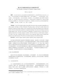
be able to display individual strings in a human-readable way. For example, Figure<br />
5-1 shows data accessed using nltk.corpus.indian.<br />
182 | Chapter 5: Categorizing and Tagging Words
If the corpus is also segmented into sentences, it will have a tagged_sents() method<br />
that divides up the tagged words into sentences rather than presenting them as one big<br />
list. This will be useful when we come to developing automatic taggers, as they are<br />
trained and tested on lists of sentences, not words.<br />
A Simplified Part-of-Speech Tagset<br />
Tagged corpora use many different conventions for tagging words. To help us get started,<br />
we will be looking at a simplified tagset (shown in Table 5-1).<br />
Table 5-1. Simplified part-of-speech tagset<br />
Tag Meaning Examples<br />
ADJ adjective new, good, high, special, big, local<br />
ADV adverb really, already, still, early, now<br />
CNJ conjunction and, or, but, if, while, although<br />
DET determiner the, a, some, most, every, no<br />
EX existential there, there’s<br />
FW foreign word dolce, ersatz, esprit, quo, maitre<br />
MOD modal verb will, can, would, may, must, should<br />
N noun year, home, costs, time, education<br />
NP proper noun Alison, Africa, April, Washington<br />
NUM number twenty-four, fourth, 1991, 14:24<br />
PRO pronoun he, their, her, its, my, I, us<br />
P preposition on, of, at, with, by, into, under<br />
TO the word to to<br />
UH interjection ah, bang, ha, whee, hmpf, oops<br />
V verb is, has, get, do, make, see, run<br />
VD past tense said, took, told, made, asked<br />
VG present participle making, going, playing, working<br />
VN past participle given, taken, begun, sung<br />
WH wh determiner who, which, when, what, where, how<br />
5.2 Tagged Corpora | 183
Figure 5-1. POS tagged data from four Indian languages: Bangla, Hindi, Marathi, and Telugu.<br />
Let’s see which of these tags are the most common in the news category of the Brown<br />
Corpus:<br />
>>> from nltk.corpus import brown<br />
>>> brown_news_tagged = brown.tagged_words(categories='news', simplify_tags=True)<br />
>>> tag_fd = nltk.FreqDist(tag for (word, tag) in brown_news_tagged)<br />
>>> tag_fd.keys()<br />
['N', 'P', 'DET', 'NP', 'V', 'ADJ', ',', '.', 'CNJ', 'PRO', 'ADV', 'VD', ...]<br />
Your Turn: Plot the frequency distribution just shown using<br />
tag_fd.plot(cumulative=True). What percentage of words are tagged<br />
using the first five tags of the above list?<br />
We can use these tags to do powerful searches using a graphical POS-concordance tool<br />
nltk.app.concordance(). Use it to search for any combination of words and POS tags,<br />
e.g., N N N N, hit/VD, hit/VN, or the ADJ man.<br />
Nouns<br />
Nouns generally refer to people, places, things, or concepts, e.g., woman, Scotland,<br />
book, intelligence. Nouns can appear after determiners and adjectives, and can be the<br />
subject or object of the verb, as shown in Table 5-2.<br />
Table 5-2. Syntactic patterns involving some nouns<br />
Word After a determiner Subject of the verb<br />
woman the woman who I saw yesterday ... the woman sat down<br />
Scotland the Scotland I remember as a child ... Scotland has five million people<br />
book the book I bought yesterday ... this book recounts the colonization of Australia<br />
intelligence the intelligence displayed by the child ... Mary’s intelligence impressed her teachers<br />
The simplified noun tags are N for common nouns like book, and NP for proper nouns<br />
like Scotland.<br />
184 | Chapter 5: Categorizing and Tagging Words
Let’s inspect some tagged text to see what parts-of-speech occur before a noun, with<br />
the most frequent ones first. To begin with, we construct a list of bigrams whose members<br />
are themselves word-tag pairs, such as (('The', 'DET'), ('Fulton', 'NP')) and<br />
(('Fulton', 'NP'), ('County', 'N')). Then we construct a FreqDist from the tag parts<br />
of the bigrams.<br />
>>> word_tag_pairs = nltk.bigrams(brown_news_tagged)<br />
>>> list(nltk.FreqDist(a[1] for (a, b) in word_tag_pairs if b[1] == 'N'))<br />
['DET', 'ADJ', 'N', 'P', 'NP', 'NUM', 'V', 'PRO', 'CNJ', '.', ',', 'VG', 'VN', ...]<br />
This confirms our assertion that nouns occur after determiners and adjectives, including<br />
numeral adjectives (tagged as NUM).<br />
Verbs<br />
Verbs are words that describe events and actions, e.g., fall and eat, as shown in Table<br />
5-3. In the context of a sentence, verbs typically express a relation involving the<br />
referents of one or more noun phrases.<br />
Table 5-3. Syntactic patterns involving some verbs<br />
Word Simple With modifiers and adjuncts (italicized)<br />
fall Rome fell Dot com stocks suddenly fell like a stone<br />
eat Mice eat cheese John ate the pizza with gusto<br />
What are the most common verbs in news text? Let’s sort all the verbs by frequency:<br />
>>> wsj = nltk.corpus.treebank.tagged_words(simplify_tags=True)<br />
>>> word_tag_fd = nltk.FreqDist(wsj)<br />
>>> [word + "/" + tag for (word, tag) in word_tag_fd if tag.startswith('V')]<br />
['is/V', 'said/VD', 'was/VD', 'are/V', 'be/V', 'has/V', 'have/V', 'says/V',<br />
'were/VD', 'had/VD', 'been/VN', "'s/V", 'do/V', 'say/V', 'make/V', 'did/VD',<br />
'rose/VD', 'does/V', 'expected/VN', 'buy/V', 'take/V', 'get/V', 'sell/V',<br />
'help/V', 'added/VD', 'including/VG', 'according/VG', 'made/VN', 'pay/V', ...]<br />
Note that the items being counted in the frequency distribution are word-tag pairs.<br />
Since words and tags are paired, we can treat the word as a condition and the tag as an<br />
event, and initialize a conditional frequency distribution with a list of condition-event<br />
pairs. This lets us see a frequency-ordered list of tags given a word:<br />
>>> cfd1 = nltk.ConditionalFreqDist(wsj)<br />
>>> cfd1['yield'].keys()<br />
['V', 'N']<br />
>>> cfd1['cut'].keys()<br />
['V', 'VD', 'N', 'VN']<br />
We can reverse the order of the pairs, so that the tags are the conditions, and the words<br />
are the events. Now we can see likely words for a given tag:<br />
5.2 Tagged Corpora | 185
cfd2 = nltk.ConditionalFreqDist((tag, word) for (word, tag) in wsj)<br />
>>> cfd2['VN'].keys()<br />
['been', 'expected', 'made', 'compared', 'based', 'priced', 'used', 'sold',<br />
'named', 'designed', 'held', 'fined', 'taken', 'paid', 'traded', 'said', ...]<br />
To clarify the distinction between VD (past tense) and VN (past participle), let’s find<br />
words that can be both VD and VN, and see some surrounding text:<br />
>>> [w for w in cfd1.conditions() if 'VD' in cfd1[w] and 'VN' in cfd1[w]]<br />
['Asked', 'accelerated', 'accepted', 'accused', 'acquired', 'added', 'adopted', ...]<br />
>>> idx1 = wsj.index(('kicked', 'VD'))<br />
>>> wsj[idx1-4:idx1+1]<br />
[('While', 'P'), ('program', 'N'), ('trades', 'N'), ('swiftly', 'ADV'),<br />
('kicked', 'VD')]<br />
>>> idx2 = wsj.index(('kicked', 'VN'))<br />
>>> wsj[idx2-4:idx2+1]<br />
[('head', 'N'), ('of', 'P'), ('state', 'N'), ('has', 'V'), ('kicked', 'VN')]<br />
In this case, we see that the past participle of kicked is preceded by a form of the auxiliary<br />
verb have. Is this generally true?<br />
Your Turn: Given the list of past participles specified by<br />
cfd2['VN'].keys(), try to collect a list of all the word-tag pairs that immediately<br />
precede items in that list.<br />
Adjectives and Adverbs<br />
Two other important word classes are adjectives and adverbs. Adjectives describe<br />
nouns, and can be used as modifiers (e.g., large in the large pizza), or as predicates (e.g.,<br />
the pizza is large). English adjectives can have internal structure (e.g., fall+ing in the<br />
falling stocks). Adverbs modify verbs to specify the time, manner, place, or direction of<br />
the event described by the verb (e.g., quickly in the stocks fell quickly). Adverbs may<br />
also modify adjectives (e.g., really in Mary’s teacher was really nice).<br />
English has several categories of closed class words in addition to prepositions, such<br />
as articles (also often called determiners) (e.g., the, a), modals (e.g., should, may),<br />
and personal pronouns (e.g., she, they). Each dictionary and grammar classifies these<br />
words differently.<br />
Your Turn: If you are uncertain about some of these parts-of-speech,<br />
study them using nltk.app.concordance(), or watch some of the Schoolhouse<br />
Rock! grammar videos available at YouTube, or consult Section<br />
5.9.<br />
186 | Chapter 5: Categorizing and Tagging Words
Unsimplified Tags<br />
Let’s find the most frequent nouns of each noun part-of-speech type. The program in<br />
Example 5-1 finds all tags starting with NN, and provides a few example words for each<br />
one. You will see that there are many variants of NN; the most important contain $ for<br />
possessive nouns, S for plural nouns (since plural nouns typically end in s), and P for<br />
proper nouns. In addition, most of the tags have suffix modifiers: -NC for citations,<br />
-HL for words in headlines, and -TL for titles (a feature of Brown tags).<br />
Example 5-1. Program to find the most frequent noun tags.<br />
def findtags(tag_prefix, tagged_text):<br />
cfd = nltk.ConditionalFreqDist((tag, word) for (word, tag) in tagged_text<br />
if tag.startswith(tag_prefix))<br />
return dict((tag, cfd[tag].keys()[:5]) for tag in cfd.conditions())<br />
>>> tagdict = findtags('NN', nltk.corpus.brown.tagged_words(categories='news'))<br />
>>> for tag in sorted(tagdict):<br />
... print tag, tagdict[tag]<br />
...<br />
NN ['year', 'time', 'state', 'week', 'man']<br />
NN$ ["year's", "world's", "state's", "nation's", "company's"]<br />
NN$-HL ["Golf's", "Navy's"]<br />
NN$-TL ["President's", "University's", "League's", "Gallery's", "Army's"]<br />
NN-HL ['cut', 'Salary', 'condition', 'Question', 'business']<br />
NN-NC ['eva', 'ova', 'aya']<br />
NN-TL ['President', 'House', 'State', 'University', 'City']<br />
NN-TL-HL ['Fort', 'City', 'Commissioner', 'Grove', 'House']<br />
NNS ['years', 'members', 'people', 'sales', 'men']<br />
NNS$ ["children's", "women's", "men's", "janitors'", "taxpayers'"]<br />
NNS$-HL ["Dealers'", "Idols'"]<br />
NNS$-TL ["Women's", "States'", "Giants'", "Officers'", "Bombers'"]<br />
NNS-HL ['years', 'idols', 'Creations', 'thanks', 'centers']<br />
NNS-TL ['States', 'Nations', 'Masters', 'Rules', 'Communists']<br />
NNS-TL-HL ['Nations']<br />
When we come to constructing part-of-speech taggers later in this chapter, we will use<br />
the unsimplified tags.<br />
Exploring Tagged Corpora<br />
Let’s briefly return to the kinds of exploration of corpora we saw in previous chapters,<br />
this time exploiting POS tags.<br />
Suppose we’re studying the word often and want to see how it is used in text. We could<br />
ask to see the words that follow often:<br />
>>> brown_learned_text = brown.words(categories='learned')<br />
>>> sorted(set(b for (a, b) in nltk.ibigrams(brown_learned_text) if a == 'often'))<br />
[',', '.', 'accomplished', 'analytically', 'appear', 'apt', 'associated', 'assuming',<br />
'became', 'become', 'been', 'began', 'call', 'called', 'carefully', 'chose', ...]<br />
However, it’s probably more instructive use the tagged_words() method to look at the<br />
part-of-speech tag of the following words:<br />
5.2 Tagged Corpora | 187
own_lrnd_tagged = brown.tagged_words(categories='learned', simplify_tags=True)<br />
>>> tags = [b[1] for (a, b) in nltk.ibigrams(brown_lrnd_tagged) if a[0] == 'often']<br />
>>> fd = nltk.FreqDist(tags)<br />
>>> fd.tabulate()<br />
VN V VD DET ADJ ADV P CNJ , TO VG WH VBZ .<br />
15 12 8 5 5 4 4 3 3 1 1 1 1 1<br />
Notice that the most high-frequency parts-of-speech following often are verbs. Nouns<br />
never appear in this position (in this particular corpus).<br />
Next, let’s look at some larger context, and find words involving particular sequences<br />
of tags and words (in this case " to "). In Example 5-2, we consider each<br />
three-word window in the sentence , and check whether they meet our criterion .<br />
If the tags match, we print the corresponding words .<br />
Example 5-2. Searching for three-word phrases using POS tags.<br />
from nltk.corpus import brown<br />
def process(sentence):<br />
for (w1,t1), (w2,t2), (w3,t3) in nltk.trigrams(sentence):<br />
if (t1.startswith('V') and t2 == 'TO' and t3.startswith('V')):<br />
print w1, w2, w3<br />
>>> for tagged_sent in brown.tagged_sents():<br />
... process(tagged_sent)<br />
...<br />
combined to achieve<br />
continue to place<br />
serve to protect<br />
wanted to wait<br />
allowed to place<br />
expected to become<br />
...<br />
Finally, let’s look for words that are highly ambiguous as to their part-of-speech tag.<br />
Understanding why such words are tagged as they are in each context can help us clarify<br />
the distinctions between the tags.<br />
>>> brown_news_tagged = brown.tagged_words(categories='news', simplify_tags=True)<br />
>>> data = nltk.ConditionalFreqDist((word.lower(), tag)<br />
... for (word, tag) in brown_news_tagged)<br />
>>> for word in data.conditions():<br />
... if len(data[word]) > 3:<br />
... tags = data[word].keys()<br />
... print word, ' '.join(tags)<br />
...<br />
best ADJ ADV NP V<br />
better ADJ ADV V DET<br />
close ADV ADJ V N<br />
cut V N VN VD<br />
even ADV DET ADJ V<br />
grant NP N V -<br />
hit V VD VN N<br />
lay ADJ V NP VD<br />
left VD ADJ N VN<br />
188 | Chapter 5: Categorizing and Tagging Words
like CNJ V ADJ P -<br />
near P ADV ADJ DET<br />
open ADJ V N ADV<br />
past N ADJ DET P<br />
present ADJ ADV V N<br />
read V VN VD NP<br />
right ADJ N DET ADV<br />
second NUM ADV DET N<br />
set VN V VD N -<br />
that CNJ V WH DET<br />
Your Turn: Open the POS concordance tool nltk.app.concordance()<br />
and load the complete Brown Corpus (simplified tagset). Now pick<br />
some of the words listed at the end of the previous code example and<br />
see how the tag of the word correlates with the context of the word. E.g.,<br />
search for near to see all forms mixed together, near/ADJ to see it used<br />
as an adjective, near N to see just those cases where a noun follows, and<br />
so forth.<br />
5.3 Mapping Words to Properties Using Python <strong>Dictionaries</strong><br />
As we have seen, a tagged word of the form (word, tag) is an association between a<br />
word and a part-of-speech tag. Once we start doing part-of-speech tagging, we will be<br />
creating programs that assign a tag to a word, the tag which is most likely in a given<br />
context. We can think of this process as mapping from words to tags. The most natural<br />
way to store mappings in Python uses the so-called dictionary data type (also known<br />
as an associative array or hash array in other programming languages). In this section,<br />
we look at dictionaries and see how they can represent a variety of language information,<br />
including parts-of-speech.<br />
Indexing Lists Versus <strong>Dictionaries</strong><br />
A text, as we have seen, is treated in Python as a list of words. An important property<br />
of lists is that we can “look up” a particular item by giving its index, e.g., text1[100].<br />
Notice how we specify a number and get back a word. We can think of a list as a simple<br />
kind of table, as shown in Figure 5-2.<br />
Figure 5-2. List lookup: We access the contents of a Python list with the help of an integer index.<br />
5.3 Mapping Words to Properties Using Python <strong>Dictionaries</strong> | 189
Contrast this situation with frequency distributions (Section 1.3), where we specify a<br />
word and get back a number, e.g., fdist['monstrous'], which tells us the number of<br />
times a given word has occurred in a text. Lookup using words is familiar to anyone<br />
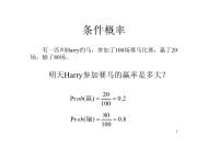
who has used a dictionary. Some more examples are shown in Figure 5-3.<br />
Figure 5-3. Dictionary lookup: we access the entry of a dictionary using a key such as someone’s name,<br />
a web domain, or an English word; other names for dictionary are map, hashmap, hash, and<br />
associative array.<br />
In the case of a phonebook, we look up an entry using a name and get back a number.<br />
When we type a domain name in a web browser, the computer looks this up to get<br />
back an IP address. A word frequency table allows us to look up a word and find its<br />
frequency in a text collection. In all these cases, we are mapping from names to numbers,<br />
rather than the other way around as with a list. In general, we would like to be<br />
able to map between arbitrary types of information. Table 5-4 lists a variety of linguistic<br />
objects, along with what they map.<br />
Table 5-4. Linguistic objects as mappings from keys to values<br />
Linguistic object Maps from Maps to<br />
Document Index Word List of pages (where word is found)<br />
Thesaurus Word sense List of synonyms<br />
Dictionary Headword Entry (part-of-speech, sense definitions, etymology)<br />
Comparative Wordlist Gloss term Cognates (list of words, one per language)<br />
Morph Analyzer Surface form Morphological analysis (list of component morphemes)<br />
Most often, we are mapping from a “word” to some structured object. For example, a<br />
document index maps from a word (which we can represent as a string) to a list of pages<br />
(represented as a list of integers). In this section, we will see how to represent such<br />
mappings in Python.<br />
<strong>Dictionaries</strong> in Python<br />
Python provides a dictionary data type that can be used for mapping between arbitrary<br />
types. It is like a conventional dictionary, in that it gives you an efficient way to look<br />
things up. However, as we see from Table 5-4, it has a much wider range of uses.<br />
190 | Chapter 5: Categorizing and Tagging Words
To illustrate, we define pos to be an empty dictionary and then add four entries to it,<br />
specifying the part-of-speech of some words. We add entries to a dictionary using the<br />
familiar square bracket notation:<br />
>>> pos = {}<br />
>>> pos<br />
{}<br />
>>> pos['colorless'] = 'ADJ'<br />
>>> pos<br />
{'colorless': 'ADJ'}<br />
>>> pos['ideas'] = 'N'<br />
>>> pos['sleep'] = 'V'<br />
>>> pos['furiously'] = 'ADV'<br />
>>> pos<br />
{'furiously': 'ADV', 'ideas': 'N', 'colorless': 'ADJ', 'sleep': 'V'}<br />
So, for example, says that the part-of-speech of colorless is adjective, or more specifically,<br />
that the key 'colorless' is assigned the value 'ADJ' in dictionary pos. When<br />
we inspect the value of pos we see a set of key-value pairs. Once we have populated<br />
the dictionary in this way, we can employ the keys to retrieve values:<br />
>>> pos['ideas']<br />
'N'<br />
>>> pos['colorless']<br />
'ADJ'<br />
Of course, we might accidentally use a key that hasn’t been assigned a value.<br />
>>> pos['green']<br />
Traceback (most recent call last):<br />
File "", line 1, in ?<br />
KeyError: 'green'<br />
This raises an important question. Unlike lists and strings, where we can use len() to<br />
work out which integers will be legal indexes, how do we work out the legal keys for a<br />
dictionary? If the dictionary is not too big, we can simply inspect its contents by evaluating<br />
the variable pos. As we saw earlier in line , this gives us the key-value pairs.<br />
Notice that they are not in the same order they were originally entered; this is because<br />
dictionaries are not sequences but mappings (see Figure 5-3), and the keys are not<br />
inherently ordered.<br />
Alternatively, to just find the keys, we can either convert the dictionary to a list or<br />
use the dictionary in a context where a list is expected, as the parameter of sorted()<br />
or in a for loop .<br />
>>> list(pos)<br />
['ideas', 'furiously', 'colorless', 'sleep']<br />
>>> sorted(pos)<br />
['colorless', 'furiously', 'ideas', 'sleep']<br />
>>> [w for w in pos if w.endswith('s')]<br />
['colorless', 'ideas']<br />
5.3 Mapping Words to Properties Using Python <strong>Dictionaries</strong> | 191
When you type list(pos), you might see a different order to the one<br />
shown here. If you want to see the keys in order, just sort them.<br />
As well as iterating over all keys in the dictionary with a for loop, we can use the for<br />
loop as we did for printing lists:<br />
>>> for word in sorted(pos):<br />
... print word + ":", pos[word]<br />
...<br />
colorless: ADJ<br />
furiously: ADV<br />
sleep: V<br />
ideas: N<br />
Finally, the dictionary methods keys(), values(), and items() allow us to access the<br />
keys, values, and key-value pairs as separate lists. We can even sort tuples , which<br />
orders them according to their first element (and if the first elements are the same, it<br />
uses their second elements).<br />
>>> pos.keys()<br />
['colorless', 'furiously', 'sleep', 'ideas']<br />
>>> pos.values()<br />
['ADJ', 'ADV', 'V', 'N']<br />
>>> pos.items()<br />
[('colorless', 'ADJ'), ('furiously', 'ADV'), ('sleep', 'V'), ('ideas', 'N')]<br />
>>> for key, val in sorted(pos.items()):<br />
... print key + ":", val<br />
...<br />
colorless: ADJ<br />
furiously: ADV<br />
ideas: N<br />
sleep: V<br />
We want to be sure that when we look something up in a dictionary, we get only one<br />
value for each key. Now suppose we try to use a dictionary to store the fact that the<br />
word sleep can be used as both a verb and a noun:<br />
>>> pos['sleep'] = 'V'<br />
>>> pos['sleep']<br />
'V'<br />
>>> pos['sleep'] = 'N'<br />
>>> pos['sleep']<br />
'N'<br />
Initially, pos['sleep'] is given the value 'V'. But this is immediately overwritten with<br />
the new value, 'N'. In other words, there can be only one entry in the dictionary for<br />
'sleep'. However, there is a way of storing multiple values in that entry: we use a list<br />
value, e.g., pos['sleep'] = ['N', 'V']. In fact, this is what we saw in Section 2.4 for<br />
the CMU Pronouncing Dictionary, which stores multiple pronunciations for a single<br />
word.<br />
192 | Chapter 5: Categorizing and Tagging Words
Defining <strong>Dictionaries</strong><br />
We can use the same key-value pair format to create a dictionary. There are a couple<br />
of ways to do this, and we will normally use the first:<br />
>>> pos = {'colorless': 'ADJ', 'ideas': 'N', 'sleep': 'V', 'furiously': 'ADV'}<br />
>>> pos = dict(colorless='ADJ', ideas='N', sleep='V', furiously='ADV')<br />
Note that dictionary keys must be immutable types, such as strings and tuples. If we<br />
try to define a dictionary using a mutable key, we get a TypeError:<br />
>>> pos = {['ideas', 'blogs', 'adventures']: 'N'}<br />
Traceback (most recent call last):<br />
File "", line 1, in <br />
TypeError: list objects are unhashable<br />
Default <strong>Dictionaries</strong><br />
If we try to access a key that is not in a dictionary, we get an error. However, it’s often<br />
useful if a dictionary can automatically create an entry for this new key and give it a<br />
default value, such as zero or the empty list. Since Python 2.5, a special kind of dictionary<br />
called a defaultdict has been available. (It is provided as nltk.defaultdict for<br />
the benefit of readers who are using Python 2.4.) In order to use it, we have to supply<br />
a parameter which can be used to create the default value, e.g., int, float, str, list,<br />
dict, tuple.<br />
>>> frequency = nltk.defaultdict(int)<br />
>>> frequency['colorless'] = 4<br />
>>> frequency['ideas']<br />
0<br />
>>> pos = nltk.defaultdict(list)<br />
>>> pos['sleep'] = ['N', 'V']<br />
>>> pos['ideas']<br />
[]<br />
These default values are actually functions that convert other objects to<br />
the specified type (e.g., int("2"), list("2")). When they are called with<br />
no parameter—say, int(), list()—they return 0 and [] respectively.<br />
The preceding examples specified the default value of a dictionary entry to be the default<br />
value of a particular data type. However, we can specify any default value we like, simply<br />
by providing the name of a function that can be called with no arguments to create the<br />
required value. Let’s return to our part-of-speech example, and create a dictionary<br />
whose default value for any entry is 'N' . When we access a non-existent entry , it<br />
is automatically added to the dictionary .<br />
>>> pos = nltk.defaultdict(lambda: 'N')<br />
>>> pos['colorless'] = 'ADJ'<br />
>>> pos['blog']<br />
'N'<br />
5.3 Mapping Words to Properties Using Python <strong>Dictionaries</strong> | 193
pos.items()<br />
[('blog', 'N'), ('colorless', 'ADJ')]<br />
This example used a lambda expression, introduced in Section 4.4. This<br />
lambda expression specifies no parameters, so we call it using parentheses<br />
with no arguments. Thus, the following definitions of f and g are<br />
equivalent:<br />
>>> f = lambda: 'N'<br />
>>> f()<br />
'N'<br />
>>> def g():<br />
... return 'N'<br />
>>> g()<br />
'N'<br />
Let’s see how default dictionaries could be used in a more substantial language processing<br />
task. Many language processing tasks—including tagging—struggle to correctly<br />
process the hapaxes of a text. They can perform better with a fixed vocabulary<br />
and a guarantee that no new words will appear. We can preprocess a text to replace<br />
low-frequency words with a special “out of vocabulary” token, UNK, with the help of a<br />
default dictionary. (Can you work out how to do this without reading on?)<br />
We need to create a default dictionary that maps each word to its replacement. The<br />
most frequent n words will be mapped to themselves. Everything else will be mapped<br />
to UNK.<br />
>>> alice = nltk.corpus.gutenberg.words('carroll-alice.txt')<br />
>>> vocab = nltk.FreqDist(alice)<br />
>>> v1000 = list(vocab)[:1000]<br />
>>> mapping = nltk.defaultdict(lambda: 'UNK')<br />
>>> for v in v1000:<br />
... mapping[v] = v<br />
...<br />
>>> alice2 = [mapping[v] for v in alice]<br />
>>> alice2[:100]<br />
['UNK', 'Alice', "'", 's', 'Adventures', 'in', 'Wonderland', 'by', 'UNK', 'UNK',<br />
'UNK', 'UNK', 'CHAPTER', 'I', '.', 'UNK', 'the', 'Rabbit', '-', 'UNK', 'Alice',<br />
'was', 'beginning', 'to', 'get', 'very', 'tired', 'of', 'sitting', 'by', 'her',<br />
'sister', 'on', 'the', 'bank', ',', 'and', 'of', 'having', 'nothing', 'to', 'do',<br />
':', 'once', 'or', 'twice', 'she', 'had', 'UNK', 'into', 'the', 'book', 'her',<br />
'sister', 'was', 'UNK', ',', 'but', 'it', 'had', 'no', 'pictures', 'or', 'UNK',<br />
'in', 'it', ',', "'", 'and', 'what', 'is', 'the', 'use', 'of', 'a', 'book', ",'",<br />
'thought', 'Alice', "'", 'without', 'pictures', 'or', 'conversation', "?'", ...]<br />
>>> len(set(alice2))<br />
1001<br />
Incrementally Updating a Dictionary<br />
We can employ dictionaries to count occurrences, emulating the method for tallying<br />
words shown in Figure 1-3. We begin by initializing an empty defaultdict, then process<br />
each part-of-speech tag in the text. If the tag hasn’t been seen before, it will have a zero<br />
194 | Chapter 5: Categorizing and Tagging Words
count by default. Each time we encounter a tag, we increment its count using the +=<br />
operator (see Example 5-3).<br />
Example 5-3. Incrementally updating a dictionary, and sorting by value.<br />
>>> counts = nltk.defaultdict(int)<br />
>>> from nltk.corpus import brown<br />
>>> for (word, tag) in brown.tagged_words(categories='news'):<br />
... counts[tag] += 1<br />
...<br />
>>> counts['N']<br />
22226<br />
>>> list(counts)<br />
['FW', 'DET', 'WH', "''", 'VBZ', 'VB+PPO', "'", ')', 'ADJ', 'PRO', '*', '-', ...]<br />
>>> from operator import itemgetter<br />
>>> sorted(counts.items(), key=itemgetter(1), reverse=True)<br />
[('N', 22226), ('P', 10845), ('DET', 10648), ('NP', 8336), ('V', 7313), ...]<br />
>>> [t for t, c in sorted(counts.items(), key=itemgetter(1), reverse=True)]<br />
['N', 'P', 'DET', 'NP', 'V', 'ADJ', ',', '.', 'CNJ', 'PRO', 'ADV', 'VD', ...]<br />
The listing in Example 5-3 illustrates an important idiom for sorting a dictionary by its<br />
values, to show words in decreasing order of frequency. The first parameter of<br />
sorted() is the items to sort, which is a list of tuples consisting of a POS tag and a<br />
frequency. The second parameter specifies the sort key using a function itemget<br />
ter(). In general, itemgetter(n) returns a function that can be called on some other<br />
sequence object to obtain the nth element:<br />
>>> pair = ('NP', 8336)<br />
>>> pair[1]<br />
8336<br />
>>> itemgetter(1)(pair)<br />
8336<br />
The last parameter of sorted() specifies that the items should be returned in reverse<br />
order, i.e., decreasing values of frequency.<br />
There’s a second useful programming idiom at the beginning of Example 5-3, where<br />
we initialize a defaultdict and then use a for loop to update its values. Here’s a schematic<br />
version:<br />
>>> my_dictionary = nltk.defaultdict(function to create default value)<br />
>>> for item in sequence:<br />
... my_dictionary[item_key] is updated with information about item<br />
Here’s another instance of this pattern, where we index words according to their last<br />
two letters:<br />
>>> last_letters = nltk.defaultdict(list)<br />
>>> words = nltk.corpus.words.words('en')<br />
>>> for word in words:<br />
... key = word[-2:]<br />
... last_letters[key].append(word)<br />
...<br />
5.3 Mapping Words to Properties Using Python <strong>Dictionaries</strong> | 195
last_letters['ly']<br />
['abactinally', 'abandonedly', 'abasedly', 'abashedly', 'abashlessly', 'abbreviately',<br />
'abdominally', 'abhorrently', 'abidingly', 'abiogenetically', 'abiologically', ...]<br />
>>> last_letters['zy']<br />
['blazy', 'bleezy', 'blowzy', 'boozy', 'breezy', 'bronzy', 'buzzy', 'Chazy', ...]<br />
The following example uses the same pattern to create an anagram dictionary. (You<br />
might experiment with the third line to get an idea of why this program works.)<br />
>>> anagrams = nltk.defaultdict(list)<br />
>>> for word in words:<br />
... key = ''.join(sorted(word))<br />
... anagrams[key].append(word)<br />
...<br />
>>> anagrams['aeilnrt']<br />
['entrail', 'latrine', 'ratline', 'reliant', 'retinal', 'trenail']<br />
Since accumulating words like this is such a common task, NLTK provides a more<br />
convenient way of creating a defaultdict(list), in the form of nltk.Index():<br />
>>> anagrams = nltk.Index((''.join(sorted(w)), w) for w in words)<br />
>>> anagrams['aeilnrt']<br />
['entrail', 'latrine', 'ratline', 'reliant', 'retinal', 'trenail']<br />
nltk.Index is a defaultdict(list) with extra support for initialization.<br />
Similarly, nltk.FreqDist is essentially a defaultdict(int) with extra<br />
support for initialization (along with sorting and plotting methods).<br />
Complex Keys and Values<br />
We can use default dictionaries with complex keys and values. Let’s study the range of<br />
possible tags for a word, given the word itself and the tag of the previous word. We will<br />
see how this information can be used by a POS tagger.<br />
>>> pos = nltk.defaultdict(lambda: nltk.defaultdict(int))<br />
>>> brown_news_tagged = brown.tagged_words(categories='news', simplify_tags=True)<br />
>>> for ((w1, t1), (w2, t2)) in nltk.ibigrams(brown_news_tagged):<br />
... pos[(t1, w2)][t2] += 1<br />
...<br />
>>> pos[('DET', 'right')]<br />
defaultdict(, {'ADV': 3, 'ADJ': 9, 'N': 3})<br />
This example uses a dictionary whose default value for an entry is a dictionary (whose<br />
default value is int(), i.e., zero). Notice how we iterated over the bigrams of the tagged<br />
corpus, processing a pair of word-tag pairs for each iteration . Each time through the<br />
loop we updated our pos dictionary’s entry for (t1, w2), a tag and its following word<br />
. When we look up an item in pos we must specify a compound key , and we get<br />
back a dictionary object. A POS tagger could use such information to decide that the<br />
word right, when preceded by a determiner, should be tagged as ADJ.<br />
196 | Chapter 5: Categorizing and Tagging Words
Inverting a Dictionary<br />
<strong>Dictionaries</strong> support efficient lookup, so long as you want to get the value for any key.<br />
If d is a dictionary and k is a key, we type d[k] and immediately obtain the value. Finding<br />
a key given a value is slower and more cumbersome:<br />
>>> counts = nltk.defaultdict(int)<br />
>>> for word in nltk.corpus.gutenberg.words('milton-paradise.txt'):<br />
... counts[word] += 1<br />
...<br />
>>> [key for (key, value) in counts.items() if value == 32]<br />
['brought', 'Him', 'virtue', 'Against', 'There', 'thine', 'King', 'mortal',<br />
'every', 'been']<br />
If we expect to do this kind of “reverse lookup” often, it helps to construct a dictionary<br />
that maps values to keys. In the case that no two keys have the same value, this is an<br />
easy thing to do. We just get all the key-value pairs in the dictionary, and create a new<br />
dictionary of value-key pairs. The next example also illustrates another way of initializing<br />
a dictionary pos with key-value pairs.<br />
>>> pos = {'colorless': 'ADJ', 'ideas': 'N', 'sleep': 'V', 'furiously': 'ADV'}<br />
>>> pos2 = dict((value, key) for (key, value) in pos.items())<br />
>>> pos2['N']<br />
'ideas'<br />
Let’s first make our part-of-speech dictionary a bit more realistic and add some more<br />
words to pos using the dictionary update() method, to create the situation where multiple<br />
keys have the same value. Then the technique just shown for reverse lookup will<br />
no longer work (why not?). Instead, we have to use append() to accumulate the words<br />
for each part-of-speech, as follows:<br />
>>> pos.update({'cats': 'N', 'scratch': 'V', 'peacefully': 'ADV', 'old': 'ADJ'})<br />
>>> pos2 = nltk.defaultdict(list)<br />
>>> for key, value in pos.items():<br />
... pos2[value].append(key)<br />
...<br />
>>> pos2['ADV']<br />
['peacefully', 'furiously']<br />
Now we have inverted the pos dictionary, and can look up any part-of-speech and find<br />
all words having that part-of-speech. We can do the same thing even more simply using<br />
NLTK’s support for indexing, as follows:<br />
>>> pos2 = nltk.Index((value, key) for (key, value) in pos.items())<br />
>>> pos2['ADV']<br />
['peacefully', 'furiously']<br />
A summary of Python’s dictionary methods is given in Table 5-5.<br />
5.3 Mapping Words to Properties Using Python <strong>Dictionaries</strong> | 197
Table 5-5. Python’s dictionary methods: A summary of commonly used methods and idioms involving<br />
dictionaries<br />
Example Description<br />
d = {} Create an empty dictionary and assign it to d<br />
d[key] = value Assign a value to a given dictionary key<br />
d.keys() The list of keys of the dictionary<br />
list(d) The list of keys of the dictionary<br />
sorted(d) The keys of the dictionary, sorted<br />
key in d Test whether a particular key is in the dictionary<br />
for key in d Iterate over the keys of the dictionary<br />
d.values() The list of values in the dictionary<br />
dict([(k1,v1), (k2,v2), ...]) Create a dictionary from a list of key-value pairs<br />
d1.update(d2) Add all items from d2 to d1<br />
defaultdict(int) A dictionary whose default value is zero<br />
5.4 Automatic Tagging<br />
In the rest of this chapter we will explore various ways to automatically add part-ofspeech<br />
tags to text. We will see that the tag of a word depends on the word and its<br />
context within a sentence. For this reason, we will be working with data at the level of<br />
(tagged) sentences rather than words. We’ll begin by loading the data we will be using.<br />
>>> from nltk.corpus import brown<br />
>>> brown_tagged_sents = brown.tagged_sents(categories='news')<br />
>>> brown_sents = brown.sents(categories='news')<br />
The Default Tagger<br />
The simplest possible tagger assigns the same tag to each token. This may seem to be<br />
a rather banal step, but it establishes an important baseline for tagger performance. In<br />
order to get the best result, we tag each word with the most likely tag. Let’s find out<br />
which tag is most likely (now using the unsimplified tagset):<br />
>>> tags = [tag for (word, tag) in brown.tagged_words(categories='news')]<br />
>>> nltk.FreqDist(tags).max()<br />
'NN'<br />
Now we can create a tagger that tags everything as NN.<br />
>>> raw = 'I do not like green eggs and ham, I do not like them Sam I am!'<br />
>>> tokens = nltk.word_tokenize(raw)<br />
>>> default_tagger = nltk.DefaultTagger('NN')<br />
>>> default_tagger.tag(tokens)<br />
[('I', 'NN'), ('do', 'NN'), ('not', 'NN'), ('like', 'NN'), ('green', 'NN'),<br />
('eggs', 'NN'), ('and', 'NN'), ('ham', 'NN'), (',', 'NN'), ('I', 'NN'),<br />
198 | Chapter 5: Categorizing and Tagging Words
('do', 'NN'), ('not', 'NN'), ('like', 'NN'), ('them', 'NN'), ('Sam', 'NN'),<br />
('I', 'NN'), ('am', 'NN'), ('!', 'NN')]<br />
Unsurprisingly, this method performs rather poorly. On a typical corpus, it will tag<br />
only about an eighth of the tokens correctly, as we see here:<br />
>>> default_tagger.evaluate(brown_tagged_sents)<br />
0.13089484257215028<br />
Default taggers assign their tag to every single word, even words that have never been<br />
encountered before. As it happens, once we have processed several thousand words of<br />
English text, most new words will be nouns. As we will see, this means that default<br />
taggers can help to improve the robustness of a language processing system. We will<br />
return to them shortly.<br />
The Regular Expression Tagger<br />
The regular expression tagger assigns tags to tokens on the basis of matching patterns.<br />
For instance, we might guess that any word ending in ed is the past participle of a verb,<br />
and any word ending with ’s is a possessive noun. We can express these as a list of<br />
regular expressions:<br />
>>> patterns = [<br />
... (r'.*ing$', 'VBG'), # gerunds<br />
... (r'.*ed$', 'VBD'), # simple past<br />
... (r'.*es$', 'VBZ'), # 3rd singular present<br />
... (r'.*ould$', 'MD'), # modals<br />
... (r'.*\'s$', 'NN$'), # possessive nouns<br />
... (r'.*s$', 'NNS'), # plural nouns<br />
... (r'^-?[0-9]+(.[0-9]+)?$', 'CD'), # cardinal numbers<br />
... (r'.*', 'NN') # nouns (default)<br />
... ]<br />
Note that these are processed in order, and the first one that matches is applied. Now<br />
we can set up a tagger and use it to tag a sentence. After this step, it is correct about a<br />
fifth of the time.<br />
>>> regexp_tagger = nltk.RegexpTagger(patterns)<br />
>>> regexp_tagger.tag(brown_sents[3])<br />
[('``', 'NN'), ('Only', 'NN'), ('a', 'NN'), ('relative', 'NN'), ('handful', 'NN'),<br />
('of', 'NN'), ('such', 'NN'), ('reports', 'NNS'), ('was', 'NNS'), ('received', 'VBD'),<br />
("''", 'NN'), (',', 'NN'), ('the', 'NN'), ('jury', 'NN'), ('said', 'NN'), (',', 'NN'),<br />
('``', 'NN'), ('considering', 'VBG'), ('the', 'NN'), ('widespread', 'NN'), ...]<br />
>>> regexp_tagger.evaluate(brown_tagged_sents)<br />
0.20326391789486245<br />
The final regular expression «.*» is a catch-all that tags everything as a noun. This is<br />
equivalent to the default tagger (only much less efficient). Instead of respecifying this<br />
as part of the regular expression tagger, is there a way to combine this tagger with the<br />
default tagger? We will see how to do this shortly.<br />
5.4 Automatic Tagging | 199
The Lookup Tagger<br />
Your Turn: See if you can come up with patterns to improve the performance<br />
of the regular expression tagger just shown. (Note that Section<br />
6.1 describes a way to partially automate such work.)<br />
A lot of high-frequency words do not have the NN tag. Let’s find the hundred most<br />
frequent words and store their most likely tag. We can then use this information as the<br />
model for a “lookup tagger” (an NLTK UnigramTagger):<br />
>>> fd = nltk.FreqDist(brown.words(categories='news'))<br />
>>> cfd = nltk.ConditionalFreqDist(brown.tagged_words(categories='news'))<br />
>>> most_freq_words = fd.keys()[:100]<br />
>>> likely_tags = dict((word, cfd[word].max()) for word in most_freq_words)<br />
>>> baseline_tagger = nltk.UnigramTagger(model=likely_tags)<br />
>>> baseline_tagger.evaluate(brown_tagged_sents)<br />
0.45578495136941344<br />
It should come as no surprise by now that simply knowing the tags for the 100 most<br />
frequent words enables us to tag a large fraction of tokens correctly (nearly half, in fact).<br />
Let’s see what it does on some untagged input text:<br />
>>> sent = brown.sents(categories='news')[3]<br />
>>> baseline_tagger.tag(sent)<br />
[('``', '``'), ('Only', None), ('a', 'AT'), ('relative', None),<br />
('handful', None), ('of', 'IN'), ('such', None), ('reports', None),<br />
('was', 'BEDZ'), ('received', None), ("''", "''"), (',', ','),<br />
('the', 'AT'), ('jury', None), ('said', 'VBD'), (',', ','),<br />
('``', '``'), ('considering', None), ('the', 'AT'), ('widespread', None),<br />
('interest', None), ('in', 'IN'), ('the', 'AT'), ('election', None),<br />
(',', ','), ('the', 'AT'), ('number', None), ('of', 'IN'),<br />
('voters', None), ('and', 'CC'), ('the', 'AT'), ('size', None),<br />
('of', 'IN'), ('this', 'DT'), ('city', None), ("''", "''"), ('.', '.')]<br />
Many words have been assigned a tag of None, because they were not among the 100<br />
most frequent words. In these cases we would like to assign the default tag of NN. In<br />
other words, we want to use the lookup table first, and if it is unable to assign a tag,<br />
then use the default tagger, a process known as backoff (Section 5.5). We do this by<br />
specifying one tagger as a parameter to the other, as shown next. Now the lookup tagger<br />
will only store word-tag pairs for words other than nouns, and whenever it cannot<br />
assign a tag to a word, it will invoke the default tagger.<br />
>>> baseline_tagger = nltk.UnigramTagger(model=likely_tags,<br />
... backoff=nltk.DefaultTagger('NN'))<br />
Let’s put all this together and write a program to create and evaluate lookup taggers<br />
having a range of sizes (Example 5-4).<br />
200 | Chapter 5: Categorizing and Tagging Words
Example 5-4. Lookup tagger performance with varying model size.<br />
def performance(cfd, wordlist):<br />
lt = dict((word, cfd[word].max()) for word in wordlist)<br />
baseline_tagger = nltk.UnigramTagger(model=lt, backoff=nltk.DefaultTagger('NN'))<br />
return baseline_tagger.evaluate(brown.tagged_sents(categories='news'))<br />
def display():<br />
import pylab<br />
words_by_freq = list(nltk.FreqDist(brown.words(categories='news')))<br />
cfd = nltk.ConditionalFreqDist(brown.tagged_words(categories='news'))<br />
sizes = 2 ** pylab.arange(15)<br />
perfs = [performance(cfd, words_by_freq[:size]) for size in sizes]<br />
pylab.plot(sizes, perfs, '-bo')<br />
pylab.title('Lookup Tagger Performance with Varying Model Size')<br />
pylab.xlabel('Model Size')<br />
pylab.ylabel('Performance')<br />
pylab.show()<br />
>>> display()<br />
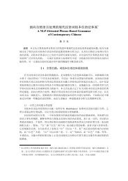
Observe in Figure 5-4 that performance initially increases rapidly as the model size<br />
grows, eventually reaching a plateau, when large increases in model size yield little<br />
improvement in performance. (This example used the pylab plotting package, discussed<br />
in Section 4.8.)<br />
Evaluation<br />
In the previous examples, you will have noticed an emphasis on accuracy scores. In<br />
fact, evaluating the performance of such tools is a central theme in NLP. Recall the<br />
processing pipeline in Figure 1-5; any errors in the output of one module are greatly<br />
multiplied in the downstream modules.<br />
We evaluate the performance of a tagger relative to the tags a human expert would<br />
assign. Since we usually don’t have access to an expert and impartial human judge, we<br />
make do instead with gold standard test data. This is a corpus which has been manually<br />
annotated and accepted as a standard against which the guesses of an automatic<br />
system are assessed. The tagger is regarded as being correct if the tag it guesses for a<br />
given word is the same as the gold standard tag.<br />
Of course, the humans who designed and carried out the original gold standard annotation<br />
were only human. Further analysis might show mistakes in the gold standard,<br />
or may eventually lead to a revised tagset and more elaborate guidelines. Nevertheless,<br />
the gold standard is by definition “correct” as far as the evaluation of an automatic<br />
tagger is concerned.<br />
5.4 Automatic Tagging | 201
Figure 5-4. Lookup tagger<br />
Developing an annotated corpus is a major undertaking. Apart from the<br />
data, it generates sophisticated tools, documentation, and practices for<br />
ensuring high-quality annotation. The tagsets and other coding schemes<br />
inevitably depend on some theoretical position that is not shared by all.<br />
However, corpus creators often go to great lengths to make their work<br />
as theory-neutral as possible in order to maximize the usefulness of their<br />
work. We will discuss the challenges of creating a corpus in Chapter 11.<br />
5.5 N-Gram Tagging<br />
Unigram Tagging<br />
Unigram taggers are based on a simple statistical algorithm: for each token, assign the<br />
tag that is most likely for that particular token. For example, it will assign the tag JJ to<br />
any occurrence of the word frequent, since frequent is used as an adjective (e.g., a frequent<br />
word) more often than it is used as a verb (e.g., I frequent this cafe). A unigram<br />
tagger behaves just like a lookup tagger (Section 5.4), except there is a more convenient<br />
202 | Chapter 5: Categorizing and Tagging Words
technique for setting it up, called training. In the following code sample, we train a<br />
unigram tagger, use it to tag a sentence, and then evaluate:<br />
>>> from nltk.corpus import brown<br />
>>> brown_tagged_sents = brown.tagged_sents(categories='news')<br />
>>> brown_sents = brown.sents(categories='news')<br />
>>> unigram_tagger = nltk.UnigramTagger(brown_tagged_sents)<br />
>>> unigram_tagger.tag(brown_sents[2007])<br />
[('Various', 'JJ'), ('of', 'IN'), ('the', 'AT'), ('apartments', 'NNS'),<br />
('are', 'BER'), ('of', 'IN'), ('the', 'AT'), ('terrace', 'NN'), ('type', 'NN'),<br />
(',', ','), ('being', 'BEG'), ('on', 'IN'), ('the', 'AT'), ('ground', 'NN'),<br />
('floor', 'NN'), ('so', 'QL'), ('that', 'CS'), ('entrance', 'NN'), ('is', 'BEZ'),<br />
('direct', 'JJ'), ('.', '.')]<br />
>>> unigram_tagger.evaluate(brown_tagged_sents)<br />
0.9349006503968017<br />
We train a UnigramTagger by specifying tagged sentence data as a parameter when we<br />
initialize the tagger. The training process involves inspecting the tag of each word and<br />
storing the most likely tag for any word in a dictionary that is stored inside the tagger.<br />
Separating the Training and Testing Data<br />
Now that we are training a tagger on some data, we must be careful not to test it on<br />
the same data, as we did in the previous example. A tagger that simply memorized its<br />
training data and made no attempt to construct a general model would get a perfect<br />
score, but would be useless for tagging new text. Instead, we should split the data,<br />
training on 90% and testing on the remaining 10%:<br />
>>> size = int(len(brown_tagged_sents) * 0.9)<br />
>>> size<br />
4160<br />
>>> train_sents = brown_tagged_sents[:size]<br />
>>> test_sents = brown_tagged_sents[size:]<br />
>>> unigram_tagger = nltk.UnigramTagger(train_sents)<br />
>>> unigram_tagger.evaluate(test_sents)<br />
0.81202033290142528<br />
Although the score is worse, we now have a better picture of the usefulness of this<br />
tagger, i.e., its performance on previously unseen text.<br />
General N-Gram Tagging<br />
When we perform a language processing task based on unigrams, we are using one<br />
item of context. In the case of tagging, we consider only the current token, in isolation<br />
from any larger context. Given such a model, the best we can do is tag each word with<br />
its a priori most likely tag. This means we would tag a word such as wind with the same<br />
tag, regardless of whether it appears in the context the wind or to wind.<br />
An n-gram tagger is a generalization of a unigram tagger whose context is the current<br />
word together with the part-of-speech tags of the n-1 preceding tokens, as shown in<br />
Figure 5-5. The tag to be chosen, t n, is circled, and the context is shaded in grey. In the<br />
example of an n-gram tagger shown in Figure 5-5, we have n=3; that is, we consider<br />
5.5 N-Gram Tagging | 203
Figure 5-5. Tagger context.<br />
the tags of the two preceding words in addition to the current word. An n-gram tagger<br />
picks the tag that is most likely in the given context.<br />
A 1-gram tagger is another term for a unigram tagger: i.e., the context<br />
used to tag a token is just the text of the token itself. 2-gram taggers are<br />
also called bigram taggers, and 3-gram taggers are called trigram taggers.<br />
The NgramTagger class uses a tagged training corpus to determine which part-of-speech<br />
tag is most likely for each context. Here we see a special case of an n-gram tagger,<br />
namely a bigram tagger. First we train it, then use it to tag untagged sentences:<br />
>>> bigram_tagger = nltk.BigramTagger(train_sents)<br />
>>> bigram_tagger.tag(brown_sents[2007])<br />
[('Various', 'JJ'), ('of', 'IN'), ('the', 'AT'), ('apartments', 'NNS'),<br />
('are', 'BER'), ('of', 'IN'), ('the', 'AT'), ('terrace', 'NN'),<br />
('type', 'NN'), (',', ','), ('being', 'BEG'), ('on', 'IN'), ('the', 'AT'),<br />
('ground', 'NN'), ('floor', 'NN'), ('so', 'CS'), ('that', 'CS'),<br />
('entrance', 'NN'), ('is', 'BEZ'), ('direct', 'JJ'), ('.', '.')]<br />
>>> unseen_sent = brown_sents[4203]<br />
>>> bigram_tagger.tag(unseen_sent)<br />
[('The', 'AT'), ('population', 'NN'), ('of', 'IN'), ('the', 'AT'), ('Congo', 'NP'),<br />
('is', 'BEZ'), ('13.5', None), ('million', None), (',', None), ('divided', None),<br />
('into', None), ('at', None), ('least', None), ('seven', None), ('major', None),<br />
('``', None), ('culture', None), ('clusters', None), ("''", None), ('and', None),<br />
('innumerable', None), ('tribes', None), ('speaking', None), ('400', None),<br />
('separate', None), ('dialects', None), ('.', None)]<br />
Notice that the bigram tagger manages to tag every word in a sentence it saw during<br />
training, but does badly on an unseen sentence. As soon as it encounters a new word<br />
(i.e., 13.5), it is unable to assign a tag. It cannot tag the following word (i.e., million),<br />
even if it was seen during training, simply because it never saw it during training with<br />
a None tag on the previous word. Consequently, the tagger fails to tag the rest of the<br />
sentence. Its overall accuracy score is very low:<br />
>>> bigram_tagger.evaluate(test_sents)<br />
0.10276088906608193<br />
204 | Chapter 5: Categorizing and Tagging Words
As n gets larger, the specificity of the contexts increases, as does the chance that the<br />
data we wish to tag contains contexts that were not present in the training data. This<br />
is known as the sparse data problem, and is quite pervasive in NLP. As a consequence,<br />
there is a trade-off between the accuracy and the coverage of our results (and this is<br />
related to the precision/recall trade-off in information retrieval).<br />
Caution!<br />
Combining Taggers<br />
N-gram taggers should not consider context that crosses a sentence<br />
boundary. Accordingly, NLTK taggers are designed to work with lists<br />
of sentences, where each sentence is a list of words. At the start of a<br />
sentence, t n-1 and preceding tags are set to None.<br />
One way to address the trade-off between accuracy and coverage is to use the more<br />
accurate algorithms when we can, but to fall back on algorithms with wider coverage<br />
when necessary. For example, we could combine the results of a bigram tagger, a<br />
unigram tagger, and a default tagger, as follows:<br />
1. Try tagging the token with the bigram tagger.<br />
2. If the bigram tagger is unable to find a tag for the token, try the unigram tagger.<br />
3. If the unigram tagger is also unable to find a tag, use a default tagger.<br />
Most NLTK taggers permit a backoff tagger to be specified. The backoff tagger may<br />
itself have a backoff tagger:<br />
>>> t0 = nltk.DefaultTagger('NN')<br />
>>> t1 = nltk.UnigramTagger(train_sents, backoff=t0)<br />
>>> t2 = nltk.BigramTagger(train_sents, backoff=t1)<br />
>>> t2.evaluate(test_sents)<br />
0.84491179108940495<br />
Your Turn: Extend the preceding example by defining a TrigramTag<br />
ger called t3, which backs off to t2.<br />
Note that we specify the backoff tagger when the tagger is initialized so that training<br />
can take advantage of the backoff tagger. Thus, if the bigram tagger would assign the<br />
same tag as its unigram backoff tagger in a certain context, the bigram tagger discards<br />
the training instance. This keeps the bigram tagger model as small as possible. We can<br />
further specify that a tagger needs to see more than one instance of a context in order<br />
to retain it. For example, nltk.BigramTagger(sents, cutoff=2, backoff=t1) will discard<br />
contexts that have only been seen once or twice.<br />
5.5 N-Gram Tagging | 205
Tagging Unknown Words<br />
Our approach to tagging unknown words still uses backoff to a regular expression<br />
tagger or a default tagger. These are unable to make use of context. Thus, if our tagger<br />
encountered the word blog, not seen during training, it would assign it the same tag,<br />
regardless of whether this word appeared in the context the blog or to blog. How can<br />
we do better with these unknown words, or out-of-vocabulary items?<br />
A useful method to tag unknown words based on context is to limit the vocabulary of<br />
a tagger to the most frequent n words, and to replace every other word with a special<br />
word UNK using the method shown in Section 5.3. During training, a unigram tagger<br />
will probably learn that UNK is usually a noun. However, the n-gram taggers will detect<br />
contexts in which it has some other tag. For example, if the preceding word is to (tagged<br />
TO), then UNK will probably be tagged as a verb.<br />
Storing Taggers<br />
Training a tagger on a large corpus may take a significant time. Instead of training a<br />
tagger every time we need one, it is convenient to save a trained tagger in a file for later<br />
reuse. Let’s save our tagger t2 to a file t2.pkl:<br />
>>> from cPickle import dump<br />
>>> output = open('t2.pkl', 'wb')<br />
>>> dump(t2, output, -1)<br />
>>> output.close()<br />
Now, in a separate Python process, we can load our saved tagger:<br />
>>> from cPickle import load<br />
>>> input = open('t2.pkl', 'rb')<br />
>>> tagger = load(input)<br />
>>> input.close()<br />
Now let’s check that it can be used for tagging:<br />
>>> text = """The board's action shows what free enterprise<br />
... is up against in our complex maze of regulatory laws ."""<br />
>>> tokens = text.split()<br />
>>> tagger.tag(tokens)<br />
[('The', 'AT'), ("board's", 'NN$'), ('action', 'NN'), ('shows', 'NNS'),<br />
('what', 'WDT'), ('free', 'JJ'), ('enterprise', 'NN'), ('is', 'BEZ'),<br />
('up', 'RP'), ('against', 'IN'), ('in', 'IN'), ('our', 'PP$'), ('complex', 'JJ'),<br />
('maze', 'NN'), ('of', 'IN'), ('regulatory', 'NN'), ('laws', 'NNS'), ('.', '.')]<br />
Performance Limitations<br />
What is the upper limit to the performance of an n-gram tagger? Consider the case of<br />
a trigram tagger. How many cases of part-of-speech ambiguity does it encounter? We<br />
can determine the answer to this question empirically:<br />
206 | Chapter 5: Categorizing and Tagging Words
cfd = nltk.ConditionalFreqDist(<br />
... ((x[1], y[1], z[0]), z[1])<br />
... for sent in brown_tagged_sents<br />
... for x, y, z in nltk.trigrams(sent))<br />
>>> ambiguous_contexts = [c for c in cfd.conditions() if len(cfd[c]) > 1]<br />
>>> sum(cfd[c].N() for c in ambiguous_contexts) / cfd.N()<br />
0.049297702068029296<br />
Thus, 1 out of 20 trigrams is ambiguous. Given the current word and the previous two<br />
tags, in 5% of cases there is more than one tag that could be legitimately assigned to<br />
the current word according to the training data. Assuming we always pick the most<br />
likely tag in such ambiguous contexts, we can derive a lower bound on the performance<br />
of a trigram tagger.<br />
Another way to investigate the performance of a tagger is to study its mistakes. Some<br />
tags may be harder than others to assign, and it might be possible to treat them specially<br />
by pre- or post-processing the data. A convenient way to look at tagging errors is the<br />
confusion matrix. It charts expected tags (the gold standard) against actual tags generated<br />
by a tagger:<br />
>>> test_tags = [tag for sent in brown.sents(categories='editorial')<br />
... for (word, tag) in t2.tag(sent)]<br />
>>> gold_tags = [tag for (word, tag) in brown.tagged_words(categories='editorial')]<br />
>>> print nltk.ConfusionMatrix(gold, test)<br />
Based on such analysis we may decide to modify the tagset. Perhaps a distinction between<br />
tags that is difficult to make can be dropped, since it is not important in the<br />
context of some larger processing task.<br />
Another way to analyze the performance bound on a tagger comes from the less than<br />
100% agreement between human annotators.<br />
In general, observe that the tagging process collapses distinctions: e.g., lexical identity<br />
is usually lost when all personal pronouns are tagged PRP. At the same time, the tagging<br />
process introduces new distinctions and removes ambiguities: e.g., deal tagged as VB or<br />
NN. This characteristic of collapsing certain distinctions and introducing new distinctions<br />
is an important feature of tagging which facilitates classification and prediction.<br />
When we introduce finer distinctions in a tagset, an n-gram tagger gets more detailed<br />
information about the left-context when it is deciding what tag to assign to a particular<br />
word. However, the tagger simultaneously has to do more work to classify the current<br />
token, simply because there are more tags to choose from. Conversely, with fewer distinctions<br />
(as with the simplified tagset), the tagger has less information about context,<br />
and it has a smaller range of choices in classifying the current token.<br />
We have seen that ambiguity in the training data leads to an upper limit in tagger<br />
performance. Sometimes more context will resolve the ambiguity. In other cases, however,<br />
as noted by (Abney, 1996), the ambiguity can be resolved only with reference to<br />
syntax or to world knowledge. Despite these imperfections, part-of-speech tagging has<br />
played a central role in the rise of statistical approaches to natural language processing.<br />
In the early 1990s, the surprising accuracy of statistical taggers was a striking<br />
5.5 N-Gram Tagging | 207
demonstration that it was possible to solve one small part of the language understanding<br />
problem, namely part-of-speech disambiguation, without reference to deeper sources<br />
of linguistic knowledge. Can this idea be pushed further? In Chapter 7, we will see<br />
that it can.<br />
Tagging Across Sentence Boundaries<br />
An n-gram tagger uses recent tags to guide the choice of tag for the current word. When<br />
tagging the first word of a sentence, a trigram tagger will be using the part-of-speech<br />
tag of the previous two tokens, which will normally be the last word of the previous<br />
sentence and the sentence-ending punctuation. However, the lexical category that<br />
closed the previous sentence has no bearing on the one that begins the next sentence.<br />
To deal with this situation, we can train, run, and evaluate taggers using lists of tagged<br />
sentences, as shown in Example 5-5.<br />
Example 5-5. N-gram tagging at the sentence level.<br />
brown_tagged_sents = brown.tagged_sents(categories='news')<br />
brown_sents = brown.sents(categories='news')<br />
size = int(len(brown_tagged_sents) * 0.9)<br />
train_sents = brown_tagged_sents[:size]<br />
test_sents = brown_tagged_sents[size:]<br />
t0 = nltk.DefaultTagger('NN')<br />
t1 = nltk.UnigramTagger(train_sents, backoff=t0)<br />
t2 = nltk.BigramTagger(train_sents, backoff=t1)<br />
>>> t2.evaluate(test_sents)<br />
0.84491179108940495<br />
5.6 Transformation-Based Tagging<br />
A potential issue with n-gram taggers is the size of their n-gram table (or language<br />
model). If tagging is to be employed in a variety of language technologies deployed on<br />
mobile computing devices, it is important to strike a balance between model size and<br />
tagger performance. An n-gram tagger with backoff may store trigram and bigram tables,<br />
which are large, sparse arrays that may have hundreds of millions of entries.<br />
A second issue concerns context. The only information an n-gram tagger considers<br />
from prior context is tags, even though words themselves might be a useful source of<br />
information. It is simply impractical for n-gram models to be conditioned on the identities<br />
of words in the context. In this section, we examine Brill tagging, an inductive<br />
tagging method which performs very well using models that are only a tiny fraction of<br />
the size of n-gram taggers.<br />
Brill tagging is a kind of transformation-based learning, named after its inventor. The<br />
general idea is very simple: guess the tag of each word, then go back and fix the mistakes.<br />
208 | Chapter 5: Categorizing and Tagging Words